Optimal Universal Quantum Error Correction via Bounded Reference Frames
Abstract
Error correcting codes with a universal set of transversal gates are a desideratum for quantum computing. Such codes, however, are ruled out by the Eastin-Knill theorem. Moreover, the theorem also rules out codes which are covariant with respect to the action of transversal unitary operations forming continuous symmetries. In this work, starting from an arbitrary code, we construct approximate codes which are covariant with respect to the entire group of local unitary gates in dimension , using quantum reference frames. We show that our codes are capable of efficiently correcting different types of erasure errors. When only a small fraction of the qudits upon which the code is built are erased, our covariant code has an error that scales as , which is reminiscent of the Heisenberg limit of quantum metrology. When every qudit has a chance of being erased, our covariant code has an error that scales as . We show that the error scaling is optimal in both cases. Our approach has implications for fault-tolerant quantum computing, reference frame error correction, and the AdS-CFT duality.
I Introduction
Reliable universal quantum computation requires fault-tolerant error correction Campbell2017, the ability to correct errors with gates that are themselves noisy. Achieving such quantum error correcting codes (QECCs) is a notoriously challenging task, due to fundamental limitations such as quantum no cloning.
One of the earliest proposals to achieve fault-tolerance for universal quantum computation was the idea of implementing all the logical gates ‘transversally’ Shor1996; Gottesman2006, which is the following idea: Given a qudit logical space and an -qudit physical space, find an encoder which maps all logical gates , the group of unitaries in dimensions, to a tensor product of physical gates:
| (1) |
where is the unitary channel corresponding to logical gate , and is either the unitary channel or the identity channel, on the th physical qudit.11 1 One may feel that Eq. (1) should be relaxed to hold only for a finite, universal gate set. However, observe that since the transversality condition is preserved under gate composition, and the set of gates generated by a universal gate set is dense in , these two conditions are effectively equivalent. Therefore, in such proposals, all gates required to achieve universal computation would be realised at the physical level by applying a tensor product of local gates. This structure is naturally suited to error correction, since an error in one of the physical qudits does not easily propagate to other physical qudits — keeping errors local so that it can be efficiently corrected afterwards.
However, as shown by Easting and Knill, there cannot exist a code satisfying Eq. (1), with a finite dimensional code space that perfectly corrects local errors eastin2009restrictions. Moreover, their result actually holds more generally for any set of qudit gates which form a continuous symmetry, that is to say, any set of gates which act on qudits and form a Lie subgroup of eastin2009restrictions; woods2020continuousgroups; faist2019continuous.
The code space is simply the image, in the physical space, of the encoding map, while a code that perfectly corrects is simply one for which the decoder can correct any error and still decode perfectly any logical state :
| (2) |
The Eastin-Knill theorem does not rule out the ability to correct local errors for a non-universal set of gates, however. A case in point is the set of Clifford gates, which can be implemented transversally but lack one crucial gate in order to form a universal set. Supplementing this set with the missing gate is the idea behind one of the frontrunner proposals for universal quantum computation, using so-called ‘magic states’ bravyi2005universal. Several other schemes to relax the transversality condition also exist knill1996threshold; bombin2007topological; paetznick2013universal; jochym2014using; bombin2015gauge; yoder2016universal; Browneaay4929.
In this work, we demonstrate a different approach to circumvent the Eastin-Knill theorem. In particular, all gates can be applied transversally under various local error models in our scheme. The key ingredients are quantum reference frames and randomness. We now introduce the former before explaining their relevance to our scheme.
In physics, all observations are reported relative to a reference frame. While the reference frames have traditionally been treated according to the laws of classical physics, the usage of quantum states to encode reference frame information (a Cartesian coordinate system, for instance) in quantum superpositions has been shown to be advantageous in problems involving reference frame alignment and overcoming super-selection rules peres2001transmission; bagan2001aligning; chiribella2004efficient; bartlett2007reference; PhysRevA.69.052326; 2013Marvian; PhysRevA.78.022304. Quantum reference frames also play a crucial role in demystifying a number of controversies and paradoxes Bartlett2006; Angelo_2011; Angelo_2012; 2011.01951, in addition to unifying various different paradigms 1912.00033. There has been a renaissance very recently, due to generalisation of quantum reference frame transformations to a “superposition of coordinate transformations” which consistently describe the physics without appealing to an external, absolute reference frame Giacomini2019; 1809.05093; PhysRevLett.123.090404; Vanrietvelde2020changeof; delahamette2021perspectiveneutral; hoehn2021quantum; delaHamette2020quantumreference.
Quantum reference frames in the context of QECCs was first explored in Ref. hayden2017error, where classical idealised reference frames22 2 An idealised reference frame, also know as a “perfect” reference frame, is one whose orientation can be deterministically obtained via measurement which is contrary to a quantum reference frame whose orientation is subject to quantum uncertainty. See bartlett2007reference for definition and woods2020continuousgroups for further insight. were employed. The hypothetical setup allows for exact decoding, and does not violate the Eastin-Knill theorem due to the use of an infinite dimensional code space. While impractical due to infinite dimensionality, the approach in Ref. hayden2017error paved the way for another approach to circumvent the Eastin-Knill theorem: using finite dimensional reference frames and decoders which only recover approximately. This route was followed in Ref. woods2020continuousgroups, where finite quantum reference frames have been used to allow for a single Abelian family of transversal gates. This construction, while useful, does not allow for universal quantum computation with transversal gates.
Here we further develop this approach and design a new family of quantum reference frames to achieve QECC constructions with all logical gates being transversal. Quantum reference frames have an inherent quantum uncertainty which unavoidably leads to a small error in the decoding. Consequently, our quantum error correcting code is only approximate. On a theoretical level, this is essential to circumvent the Eastin-Knill theorem while achieving our objective of a universal quantum gate set. On a practical level, this error can be made smaller than any chosen tolerance by increasing the size of the quantum reference frame.
The physical space necessary for our implementation of the QECC consists of two parts, the computational space and the reference frame space. Roughly speaking, the computational space is where the logical information is stored and the sequence of logical gates needed for the computation are applied on various copies. The reference frames on the other hand, play the role of recording information about which gate was applied — analogously to how gyroscopes record a Cartesian coordinate system. See Fig. 1.
At an abstract level, our encoder works by choosing a quantum reference frame which can record the “coordinates” of any logical state. This is to say, states which are distinguishable by measurements under transformations of — the special group of unitary transformations in dimensions. To implement any logical gate under this encoding, we can simply apply the gate transversally on the computational space in tandem with updating our reference frames with a corresponding transformation.
However, before this paradigm can be implemented, one needs to perform the encoding — this is where the randomness comes into play. We pick a logical gate at random, apply it transversally to the computational system and a copy to the reference frame. The reference frame information is retrieved during the decoding stage via measurement.
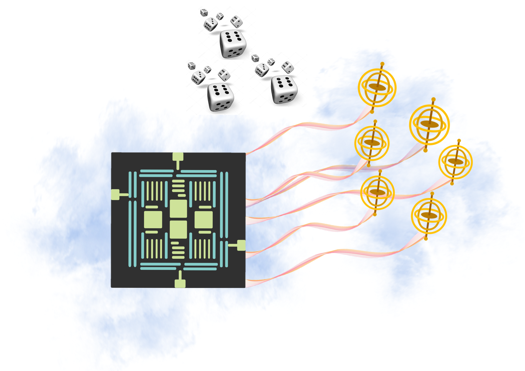
In the regime of error correction via finite quantum reference frames, the error of approximate recovery is dependent on the size of the reference frames, leading to a trade-off relation. It is thus of prime importance to identify the optimal scaling of the approximation error with respect to the size of the reference frame, so that the cost of making the recovery errors admissible can be determined. Here we analyse the error scaling of our QECC construction in two different commonly-studied error models and show that our approach is optimal in both cases. Besides the analytical analysis, we also conduct numerical simulation that further justifies our analysis in various practical error models.
In a nutshell, our contribution is to show that the use of quantum reference frames allows for approximate QECC where all gates necessary for universal quantum computation can be applied transversally, and to identify the optimal tradeoff between the approximation error and the size of the reference frames. This was the initial idea of the pioneers of quantum error correction Shor1996; Gottesman2006, who, in light of the Eastin-Knill theorem, invented distinct methods alternative to finding a transversal gate set for quantum error correction. Our work thus offers a new test bed for quantum error correction whose full potential can now be further explored. An immediate question is whether the encoder and the decoder in our construction can be implemented fault-tolerantly. As discussed in more details later, there are several paths that potentially lead to this ultimate purpose, though the concrete approach is still unknown. This is thus an important open question left for investigation in future research.
II Results
Overview. We start by introducing the relevant definitions to define our encoder, decoder, and characterisation of the decoding error. We then consider two errors models: the i.i.d. error model and the weak error model and fully characterise the performance of our QECC under these different scenarios. Details appear in the appendices.
Construction of Covariant Encoder and Decoder. A QECC is characterised by an encoder-decoder pair . The encoder is a quantum channel mapping a logical qudit, whose dimension we denote by , to a state of a physical register consisting of several qudits. The decoder corrects possible errors in the physical register and maps the state back to a logical qudit. Since our protocol uses reference frames and randomness to convert an arbitrary encoder and decoder to a covariant encoder-decoder pair, we refer to and as the subroutine encoder and decoder. The -qudit physical register is divided into two parts, the computational register C, consisting in qudits and a reference frame register R, consisting in the remaining qudits. The subroutine decoder, , maps to the computational register only.
In order to be resilient to errors, the reference frame register may consist of identical blocks, each in the quantum state . Here we choose to be an entangled state of a bipartite system (), as they offer superior performance acin2001optimal; chiribella2004efficient; chiribella2005optimal. Each part of the bipartite system further consists of several qudits. This reference frame is a finite dimensional quantum state . Rotating every qudit in the part of on by the same (unknown) unitary in (while keeping the part on unchanged) yields a state that, when measured appropriately, allows one to deduce with high accuracy. The better the quality of , the smaller the uncertainty in is.


Our covariant encoder is defined as
| (3) |
where with is the initial state of the reference frame register and is the Haar measure on . The unitary channels in Eq. (3) are defined by and the actions of an element on the computational register and the logical register, and by its action on the reference frame register (as one part of the reference frame state is rotated and the other part remains unchanged), where . See Fig. 2 for an example of how to construct the encoder.
The covariant decoder consists of first measuring the reference frame with a POVM , which yields an estimate , and then applying . Here is again the Haar measure. We then perform the subroutine decoder of the original code to correct errors, and finally we redo to obtain the final, decoded output. This gives rise to the channel
| (4) |
where the map outputs the probability density function of obtaining measurement outcome estimate .
One may be concerned about the practicality of constructing Eqs. (3) and (4), since sampling from the Haar measure is essentially to randomly apply all unitary gates, which might be computationally hard. In fact, we show later that, using the technique of unitary -designs PhysRevLett.98.130502; Dahlsten_2007; PhysRevA.80.012304; CMPHarrow; Diniz2011; PhysRevA.78.062329; CMPBrandao; PhysRevX.7.021006, we only require to sample from a discrete set of unitary gates in a computationally efficient manner.
Errors arise in this procedure both from any noise that occurs between encoder-decoder, as well as in the measurement of the reference frame itself. Nevertheless, we show that the overall error vanishes with the number of qudits upon which we construct the covariant code.
As promised, the encoder in Eq. (3) satisfies the transversality condition, Eq. (1), thanks to the well-known invariance properties of the Haar measure. In our particular case, it takes the form:
| (5) |
for any , where and , with , and the identity channel. Notice that since our decoder is also covariant, i.e. , our entire code is covariant: .
Reference Frame structure. There is a trade-off: the optimal pair of the initial reference frame state and the POVM , which yields the smallest decoding errors when no noise is present, tends not to be very resilient to noise. Conversely, those which are highly resilient to noise, tend to lead to substantial decoding errors. As such, the optimal reference frame choice depends on the noise model. We will only provide the general structure considered here, and specialise later as specific noise models are introduced.
We divide the reference frame register qudits into blocks of identical systems, i.e., and construct identical states on each of them, . Each block consists in qudits each, such that . We assume that the error occurring on each of the reference frames is detectable, i.e., it acts as follows for all : it takes the state on to an error space that is orthogonal to . This is the case, for instance, for erasure errors.
The measurement performed on the reference frame during the decoding stage, is a two step process: We first perform binary projective measurements onto and for all blocks , followed by discarding those blocks whose state is in the error space. We then measure the remaining blocks to obtain an estimate , which is used to decode the information in the computational space [see Eq. (4)].
Decoding Error and Noise Structure. There are two contributing factors to errors in our covariant scheme: noise occurring between encoding and decoding, and errors in the decoding due to the finiteness of the reference frames. Here we show that our protocol is able to recover from both of these. Since these errors hinder our ability to decode, we refer to them as decoding errors and quantify it via the diamond norm:
| (6) |
where is the noise channel being considered, and the subscript in is to remind the reader that the error is originating from making an encoder-decoder pair covariant. We assume it to be a statistical mixture over channels on the computation and reference frame registers, i.e.
| (7) |
where are channels characterising the error on the computational/reference frame register, and is a probability distribution. We also need to assume that the errors are covariant, namely for all . For example, erasure errors are of this form.
In Appendix A, we show that the total decoding error satisfies a bound of the form , where only depends on either the computational error or the reference frame error ; whichever error is dominant.
Error bounds for the Weak Error Model. Our first result concerns the case in which relatively few errors occur. Specifically, the error is that at most qudits among the qudit systems composing the computational register and the reference frame register, are randomly lost:
| (8) |
where the summation runs over all subsets of cardinality at most , and denotes the erasure of qudits whose labels are in the set , and is a probability distribution.
Any quantum error-correcting code over qudits of distance at least can perfectly correct erasures Gottesman2006. For instance, the polynomial codes of Aharonov and Ben-Or are stabilizer codes with this property aharonov_fault-tolerant_1997. In these cases, we employ one of the perfect codes as the non-covariant subroutine of our code. Since we only need to encode one logical qudit, the perfect code requires only computational qudits.
This is to say: the subroutine code we use requires only computational qudits and corrects perfectly up to erasure errors on the computational register. Next we arrange the reference frame to perform well against this type of noise. To this purpose, we set , so that the reference frames has blocks. Crucially, these conditions imply that at least one of the reference frame states will survive the erasure, and we can measure it to obtain the embedded rotation.
On each block we construct a reference frame state. Since the noise is weak, we can utilise as much entanglement as possible to enhance the accuracy of the reference frame decoding. To this purpose, we design a new family of highly coupled quantum reference frame states, which turn out to be a highly nontrivial generalisation of the sine-shape states buvzek1999optimal, and thus we name them generalised sine states. Using the generalised sine states as reference frames for our error correction protocol, we can recover the information with high accuracy. We derive an upper bound on the recovery error in our protocol for the weak error model, defined by Eq. (8):
| (9) |
All details can be found in Appendix B. Since can be chosen to be and is close to , our protocol achieves the Heisenberg limit with respect to the total number of qudit systems.
It is most challenging to correct the errors in the weak error model when the locations of the erasures are most uncertain, that is, when , and the are constant, in Eq. (8). In this worse case scenario, we can lower bound the decoding error:
| (10) |
What is more, we show that any encoder-decoder pair which satisfies the transversality condition Eq. (1), encoding one qudit into physical qudits which is subject to the weak error model (8) with maximum uncertainty as described above, has a decoding error which is lower bounded by (10). As shown in Appendix B, the derivation of Eq. (10) comes from a strengthening of a bound found in kubica2020using (see also zhou2021new for a more recent result with similar bounds). Since the bound (10) matches the performance of our protocol in scaling, we conclude that the optimal error scaling of covariant codes is .
Error bounds for the i.i.d. Error Model. We now turn our attention to types of erasure errors which are stronger than the one considered in the previous section and more realistic. The error affects each qudit independently, erasing the qudit with a probability :
| (11) |
where denotes the single-qudit erasure channel. This error model can be written in the form Eq. (7), and is thus compatible with our prior assumptions. Since the erasure channel is degradable, if the information leaked to the environment would not be retrievable. Note that, in general, the error model on each qudit does not have to be identical, and each qudit can have distinct probability of being erased. In that case, however, we can simply set to be the worst case over and consider this more stringent model instead.
In contrast to the weak error model case, there does not exist any code, which we can use for our subroutine code, that perfectly corrects the errors at hand. Instead, there exist pretty good codes that correct the error unless too many qudits are erased. The quantum capacity of the erasure channel, with erasure probability , has been determined to be bennett1997capacities. We can choose , the number of computational qudits, to grow with . When is large, since the number of qudits we want to encode is only one qudit and is much smaller than that allowed by the capacity [which is ], the error probability would vanish exponentially in .
We choose the number of computational qudits to scale sub-linearly in the total number of qudits, that is, , where does not depend on and can be chosen to be very small. We use any subroutine code that encodes one qudit into computational qudits, with the property that it has a decoding error for some that may depend on . By a random coding argument, one can show that there exists a stabilizer code satisfying our requirement (see, e.g., gottesman1997stabilizer), although its explicit form is not given. Recently, progress in error correcting codes also showed that quantum polar codes renes_efficient_2012; renes_polar_2014 and Reed-Muller codes kumar_reed-muller_2016 have the desired property. Notice that the requirement of the scaling is chosen for convenience of analysing the error, and it can be further relaxed in practice.
Meanwhile, the model is now too noisy for the highly coupled reference frame state used in the weak error model to be effective. Instead, we prepare the reference frame register to have only two qudits per block, namely , with the reference frame on each two qudits block being the maximally entangled state. While like in the weak error model, this choice means that one erasure error only destroys one reference frame block, now there are far more blocks, which reduces the chance of them all being erased. The price to pay for this more error resilient setup, is less precise reference frames, due the smaller dimension of each block.
As long as there are still order non erased blocks left we can achieve high performance, which happens with very high probability. Indeed, the overall error, Eq. (11), can be recast into the form:
| (12) |
Then the number of surviving blocks follows a binomial distribution with mean , which is sufficient for a high accuracy decoding. This reasoning leads us to the following upper bound on the decoding error under the i.i.d. error model (12): For any , there exists such that
| (13) |
for all . Details of the proof can be found in Appendix C.
The error of our protocol scales almost as , instead of in the previous case. This is a result of the (stronger) i.i.d. noise. In fact, the error scaling of our protocol is still optimal for this error model. Analogously to the weak error model, we can prove that the scaling is also optimal for the i.i.d. error model. In particular, we prove that all covariant QECC satisfy the following bound under the i.i.d. error model:
| (14) |
In the above analysis, we focused on erasure error models, as they allow us to derive analytical bounds on our protocol’s performance. Nevertheless, our protocol also performs well under other commonly encountered error types, as we show in the following.
Numerical simulation for generic error models. In addition to the above bounds, we also conduct numerical experiments to evaluate the performance of our protocol. As a working example, we use the “5-qubit code” laflamme1996perfect (5 computational qubits; one logical qubit) as the subroutine encoding and decoding pair. We consider not only erasure errors but also other common error types like dephasing errors and depolarising errors.
We first consider the weak erasure error model and use a group of identical generalised sine states as the reference frame register. We assume that at least one reference frame state survives the erasure error, which consists of qubits. (Recall that the number of qubits is always even since we use entangled reference frame states.) As shown in Fig. 3, the decoding error (in the leading order) is , matching the prediction of our theory.

We now consider errors beyond the erasure models. We first consider the case where all reference frame qubits are subject to i.i.d. depolarising/dephasing error with probability . In this case, our reference frame register consists of maximally entangled states. Each of the reference frame states are measured individually for an estimate of the reference frame parameters. We assume at most one out of the five computational qubits is subject to error (corresponding to an error rate of ), so that the logical qubit can always be recovered.
Notice that, unlike the erasure error, depolarising and dephasing errors in the reference frame register are not flagged (i.e., we do not know whether a reference frame state is subject to an error or not). In order to mitigate the effect of erroneous reference frames, we adopt a majority vote algorithm that abandons estimates in case they are likely to be faulty. With this method, for the i.i.d. depolarizing/dephasing model, we are able to achieve decoding errors (in the leading order) for the depolarising error and for the dephasing error, with being the total number of physical qubits employed in our construction (see Fig. 4). The error scaling, observed for both the i.i.d. depolarising error and the i.i.d. dephasing error, coincides with the lower bound (13) which we proved for the i.i.d. erasure error model. It suggests that the error scaling of our protocol is consistent in generic error models. We have also tested our protocol under variants of the above error models: We consider models where one fifth reference frame qubits go through the completely depolarising/dephasing error, and the error scaling has also been observed (see Table. 1 for a summary).
These results show that the application of our protocol is not limited to erasure errors. Instead, it has good potential to work well under generic error types. Our code is available at moyin2021github, and more details can be found in Appendix E.
| (total qubits) | 75 | 135 | 205 | 305 |
|---|---|---|---|---|
| i.i.d. dephasing () | 4.28e-1 | 2.58e-1 | 1.71e-1 | 1.18e-1 |
| i.i.d. depolarising () | 4.29e-1 | 2.62e-1 | 1.77e-1 | 1.27e-1 |
| 20% qubits dephased | 3.88e-1 | 2.38e-1 | 1.74e-1 | 1.20e-1 |
| 20% qubits depolarised | 4.60e-1 | 3.15e-1 | 2.18e-1 | 1.53e-1 |
| (total qubits) | 405 | 505 | 605 | 705 |
| i.i.d. dephasing () | 8.79e-2 | 7.19e-2 | 6.02e-2 | 5.09e-2 |
| i.i.d. depolarising () | 8.76e-2 | 7.32e-2 | 5.83e-2 | 5.30e-2 |
| 20% qubits dephased | 8.65e-2 | 7.03e-2 | 5.94e-2 | 5.34e-2 |
| 20% qubits depolarised | 1.21e-1 | 9.17e-2 | 7.52e-2 | 6.37e-2 |


Resource requirements and implementation. We now analyse some of the memory and time resources needed to implement our QECC which are required beyond those of the subroutine code.
Our reference frames are constructed on qudits constituting a dimensional Hilbert space. However, the reference frame states only have support on a space which we prove to be upper bounded by
| (15) |
Therefore, we can compress the reference frame state to a system of much smaller dimension, which reduces exponentially the cost of quantum memory. The cost can be further reduced at the price of a small recovery error using the compression protocols in Refs. yang2016efficient; yang2016optimal; yang2018compression.
We now turn our attention to the implementation of the covariant encoding and decoding: At first sight, our encoding and decoding may appear to necessitate sampling from the Haar measure on in order to be implemented [see Eqs. (3) and (4)]. From a computational complexity standpoint, this would be a problem, since to implement a Haar-random unitary one needs an exponential number of two-qubit gates and random bits Knill1995Haar. Fortunately, our encoding and decoding do not require sampling from the Haar measure, but rather only from a distribution which agrees with it upto the moment, for appropriate . Such equivalent distributions are known as unitary -designs PhysRevLett.98.130502; Dahlsten_2007; PhysRevA.80.012304; CMPHarrow; Diniz2011; PhysRevA.78.062329; CMPBrandao; PhysRevX.7.021006, and are more efficient to implement.
Specifically, let be a unitary representation on and be a matrix whose entries are polynomials of order in the coefficients of and of order in the coefficients of , and let be the expectation value of a function according to measure . We then say that , where denotes the Haar measure, admits a unitary -design.
Our result is that the encoder and decoder admit unitary -designs for all , . See Appendix D.1 for proof. Ref. CMPBrandao devises and quantifies a method to approximate unitary -designs: To approximate our encoder and decoder up to an error in diamond norm, it is enough to use two-qubit gates, randomly drawn from the Haar measure on . Here
| (16) | ||||
which scales polynomially in both and [recall lower bounds on , in the weak and i.i.d. error models, Eqs. (10), (14)].
Since sampling a polynomial number of times from can be performed efficiently, both the encoder and the decoder can be efficiently implemented in and so long as the reference frame state and measurement can be efficiently constructed.
Efficient error syndrome extraction. In quantum error correction, we often need to measure error syndromes after applying quantum gates. It might appear that a full decoding is needed to achieve this in our QECC, which, despite the efficiency analysis in the previous part, could have non-negligible effects on the performance of the computation. However, this is not true for the erasure error models we considered. Instead, one can keep track of the error in a very simple way and correct them all together at a suitable time.
To see this, first notice that erasure errors are “flagged”, meaning that the qudit is mapped from its original Hilbert space to an orthogonal Hilbert space . Then, the error syndrome can be obtained by a binary projective measurement consisting of projectors on and . This measurement commutes with the (covariant) implementation of logical operations, and thus to implement a sequence of logical gates we can adapt the following procedure:
- 1.
Apply .
- 2.
Create a (classical) bit string , initiated as a null vector, to record erasure errors.
- 3.
For :
- (a)
Apply ,
- (b)
measure error syndromes, and
- (c)
add the measured error locations to .
- (d)
If exceeds the maximal number of tolerable local errors, do followed by .
- (a)
- 4.
Apply .
Therefore, a full physical decoding is done only if there is too many local errors (which is determined by the subroutine code) rather than after each logical gate, making our QECC much more efficient than it appears. We remark that how this feature generalises to other error models remains an open question to be investigated in the future.
Towards fault-tolerant QECCs. To achieve practical fault tolerance, one must show that each step of the QEC procedure can be performed fault-tolerantly. For our QECC construction, the logical gate implementation is transversal and thus fault-tolerant thanks to covariance. It remains to be shown that the encoder and the decoder are both: a) computationally efficient to implement, and b) can be implemented fault tolerantly. For a), we have provided covariant encoders and decoders which can be implemented via a polynomially in (total number of physical qudits) number of two-qubit gates, while still maintaining the optimal scaling of the decoding error. Regarding b), making the encoder and the decoder fault-tolerant amounts to finding a fault-tolerant implementation of the -twirling in Eqs. (3) and (4). We remark that it is unlikely that unitary designs are the solution: Any unitary -design is an -net on the parameter space of , with vanishing in . For large , the -net becomes dense enough that, unless the commutant of has dimension larger than two, forms a universal gate set (see also (oszmaniec2020epsilon, Remark 4)). In this case, it follows that to implement the unitary design fault tolerantly we need to implement a universal gate set fault tolerantly, leading to a contradiction.
Nevertheless, unitary designs are not a must for implementing the twirling in Eqs. (3) and (4). One can, for example, use extrapolation of different noisy channels as an alternative approach. Similar ideas have resulted in error mitigation PhysRevLett.119.180509; PhysRevX.8.031027, which effectively deals with errors in near-term devices.
Another possibility, is to partition the logical space into code blocks and apply our encoding to each block individually (call this level 1 encoding). One then implements the gates corresponding to the computation such that any one gate has support on either one or two code blocks. When one wishes to implement a gate across two code blocks, these code blocks are encoded once more using our encoding scheme (call this level 2 encoding); the unitary is then implemented and we decode back to the level 1 encoding. This way, one can increase the logical code size by adding more code blocks (each one of constant size) while only applying gates on encoded states. The quantum reference frames for the level 2 encoding can be re-purposed after ever level 2 decoding for level 2 encodings over other code blocks. Using this scheme, there is a much better overall scaling of the resources involved since we no longer require twirling over the entire logical space. These possibilities will be explored more in future research. In summary, our covariant QECC construction does not immediately lead to a satisfactory approach of achieving full fault tolerance, but it opens up a new route that is worth further exploration.
III Discussion
Starting from an arbitrary error correcting code, we have shown how to use quantum reference frames to construct a new code for which all gates are covariant and transversal, up to a small error in the decoding. In the absence of noise, the error in the decoding is ultimately a consequence of the inability to perfectly determine the orientation of the reference frames via measurement.
Our results generalise the setting in woods2020continuousgroups from -dimensional reference frame representations of to -dimensional reference frame representations of . This construction is important primarily since once the logical states have been encoded, it allows for a universal set of gates to be applied transversally, which in turn can allow for errors to be more easily detected and corrected during a computation. Furthermore, the construction also allows any quantum error correcting code to be converted into a covariant code. Previously it was not known if this is possible with a finite dimensional physical space. In the setting of the weak error model and symmetry, we establish novel upper bounds on the decoding error which are tight in the scaling with (number of physical subsystems). Indeed, previous upper bounds in this context, faist2019continuous; wang2020quasi, are not tight with . Furthermore, in this context, we also improved previous results kubica2020using; zhou2021new on the lower bounds of the decoding error. We have also analysed the i.i.d. erasure model, which is more realistic in the context of computation. Here we have produced upper and lower bounds for the decoding error which are tight in the scaling with . We argued that our model for a QECC should be able to correct errors beyond those of the local erasure type. Numerical simulations of the performance of our construction for practical error models including the depolarising error and the dephasing error bears this out.
Our results also feature applications beyond correcting errors in quantum computation. Two party communication with misaligned reference frames and lossy quantum channels hayden2017error is a clear example, but the range of potential applications is much broader. In particular, we designed and introduced generalised sine states and used them as optimal reference frames in the weak error model. A characteristic novel feature of the generalised sine states is that they can achieve the Heisenberg limit in estimating a completely unknown unitary gate, making it promising to apply them in the emergent field of multiparameter quantum metrology albarelli2020perspective; gorecki2020optimal; hou2020minimal; PhysRevLett.127.110501; meyer2021variational and, more generally, in quantum information processing. Remarkably, these states have recently been used as the key to solving the long-standing optimal programming problem of unitary quantum gates Yuxiang2.
From a more fundamental physics perspective, our results provide new insight into the study of quantum gravity. In particular, there is a conjectured duality between a theory of gravity in Anti-de Sitter (AdS) space and a conformal quantum field theory (CFT) on its boundary, known as the AdS-CFT correspondence. The duality is mediated via a quantum error correcting code, where the encoding channel maps low-energy states in the Anti-de Sitter space (known as the “bulk”) to states on the conformal field (known as the “boundary”) almheiri2015bulk. The implication of the Eastin-Knill theorem, discussed in the introduction, to the AdS-CFT duality is that global continuous symmetries in the bulk cannot map onto local symmetries on the boundary (see Harlow2018a_short; Harlow2018 for details). This is often interpreted as a problem for the duality since initially such symmetries were believed to exist. It is thus interesting to quantify, as a function of physical quantities such as energy or dimension, how local symmetries of the bulk can approximate local symmetries in the boundary. This program was initiated in TamaToby; woods2020continuousgroups; faist2019continuous and is the subject of ongoing investigation (see e.g. milekhin2021quantum). Our results quantify the extent to which the approximate duality for global symmetries could exist.
Our numerical results suggest that our reference frame based QECCs work well for generic non-detectable error models. Understanding and analytically bounding the decoding error, on the other hand, requires further investigation. It would be an interesting future direction of research to rigorously analyse the performance of our QECCs in generic error models and compare to other existing constructions wang2020quasi. The dephasing error model, for example, was studied in the case in woods2020continuousgroups and shown to be correctable. This should also be true in the current case. These studies will also help pave the way to proving robustness of our results when optimised for error models found in experiments.
Finally, since our protocols only involve classical correlations between the computational system and the reference frame system, this setup is naturally suited to implementing these two physical subsystems on different quantum architectures to harness specific advantages of each platform. For example, one may wish to implement the quantum reference frames on a phonic platform using Gaussian quantum computing RevModPhys.84.621, while using superconducting qubits for the computational space.
Acknowledgements.
This work is supported by the Swiss National Science Foundation via the National Centre for Competence in Research “QSIT” as well as via project No. 200020_165843, by the National Science Foundation of China through Grant No. 11675136, by Hong Kong Research Grant Council through Grants No. 17300317 and 17300918. M.W. acknowledges funding from the Swiss National Science Foundation (AMBIZIONE Fellowship, No. PZ00P2_179914). M.Y. and G.C. acknowledge support by the John Templeton Foundation through grant 61466, The Quantum Information Structure of Spacetime (qiss.fr). The opinions expressed in this publication are those of the authors and do not necessarily reflect the views of the John Templeton Foundation. Research at the Perimeter Institute is supported by the Government of Canada through the Department of Innovation, Science and Economic Development Canada and by the Province of Ontario through the Ministry of Research, Innovation and Science.Appendix A Construction of covariant error correcting codes
A.1 Preliminary
We use the notation () to denote the Hilbert space of the reference frame register, the computational register, or the logical register. In particular, refers to a -dimensional Hilbert space. For a generic Hilbert space and a pure state , we will use the notation to denote the projector on the one-dimensional subspace spanned by . The set of quantum states will be denoted by . In this work we will focus on finite dimensional quantum systems, with .
A quantum process transforming an input system into a (possibly different) output system is called a quantum channel. A quantum channel transforming an input system with Hilbert space into an output system with Hilbert space is a completely positive trace-preserving map , where denotes the space of linear operators on . For pure channels with a single Kraus operator , i.e. unitaries or isometries, we use the shorthand .
We will use the big- notation, the big- notation, and the big- notation to characterise the asymptotic behaviour of functions. For a function , we write if there exists a constant so that for large enough , if there exists a constant so that for large enough , and if and .
We will make frequent use of a couple of basic concepts in representation theory of the special unitary group , which can be found in standard textbooks, e.g., Ref. fulton2013representation. We denote the Young diagrams by a vector33 3 For vectors, we use the bond font. with and by the irreducible representation of characterised by the Young diagram . We denote the collection of all Young diagrams with boxes and at most rows by (since the dimension is fixed throughout the paper, we often omit it). In particular, we define to be the vector whose -th entry is one and other entries are zero. By definition, corresponds to a legitimate Young diagram whose associated representation is the standard one, and we use the abbreviation . We will use the double-ket notation ( being an orthonormal basis) with being a matrix. With the double-ket notation, we denote by the maximally entangled state associated to , with being the dimension of the irreducible subspace. By this notation, refers to a maximally entangled state in , rotated by a local unitary . Unless otherwise specified, or sometimes denotes the Haar measure.
Other commonly used conventions and notations can be found in Table 2.
| Notation | Definition | Where defined |
|---|---|---|
| the set | ||
| the cardinality of set | ||
| total number of qudit systems in the code | Section A.3 | |
| number of qudits used as the reference frame | Section A.3 | |
| number of qudits in the base (non-covariant) code | Section A.3 | |
| number of reference frame state copies | Section A.2 | |
| the error of the constructed covariant code, measured by the diamond norm error | Eq. (32) | |
| the big- notation | Section A.1 | |
| the big- notation | Section A.1 | |
| the worst-case input fidelity between channels and | Eq. (17) | |
| the entanglement fidelity between channels and | Eq. (18) | |
| the diamond norm error between channels and | Eq. (20) | |
| the entanglement error between channels and | Eq. (21) |
Next we introduce a couple of measures of error and faithfulness that are used in this work. Consider two channels . For instance, can be a desired quantum gate and is an approximation of . Therefore, we often need measures to quantify their distance (i.e. measures of simulation error) and similarity (i.e. measures of simulation faithfulness).
The first measure of faithfulness, defined intuitively as the minimum fidelity between the outputs for the same input, is the worst-case input (or minimum) fidelity:
| (17) |
where is the Uhlmann fidelity defined for two arbitrary quantum states and and is an arbitrary reference Hilbert space. Later we give a semidefinite program to compute (see Lemma 6). Nonetheless, the worst-case fidelity is often difficult to work with, and thus it is more common to consider another measure of faithfulness, known as the entanglement fidelity raginsky2001fidelity:
| (18) |
where with being the maximally entangled state of the system and a reference. It is straightforward by definition that .
On the other hand, one can also quantify the performance of simulation by error measures. Similarly as for faithfulness, there are also two commonly considered measures of error, defined with respect to the worst-case input and the maximally entangled state. The first is the worst-case input error, or the diamond norm error, defined as:
| (19) | ||||
| (20) |
where is the trace norm and denotes the diamond norm kitaev1997quantum. Correspondingly, we have the entanglement error:
| (21) |
Again, by definition, we have .
The above faithfulness measures and error measures are not independent gilchrist2005distance. For instance, the well-known Fuchs-van de Graaf inequalities fuchs1999cryptographic, which relate fidelities to distances as
| (22) |
can be readily employed. Besides, the worst-case input error can be bounded using the following inequality
| (23) |
where is the dimension of the system (watrous2018theory, Exercise 3.6).
A.2 Quantum reference frames
In this subsection we introduce quantum reference frames, which will be the key ingredient of our construction of covariant error correcting codes. We will consider entangled reference frames, as they offer superior performance acin2001optimal; chiribella2004efficient; chiribella2005optimal. A quantum reference frame is essentially an entangled state , constructed on qudits and shared by two parties Alice and Bob. Assume that the reference frames of Alice and Bob are misaligned up to a rotation : If Bob prepares one of his qudits in, say, a state in the computational basis, it would actually be a rotated version of the corresponding state on Alice’s side, i.e., .
To align their reference frames, Bob sends his part of the state through a distortion-free channel to Bob. Now, Alice has full disposal of the bipartite state , where is the state when there is no reference frame misalignment. By making a suitable measurement, Alice obtains information on the misalignment to a good precision.
In this work, we will mainly use a quantum reference frame in a single-party but mathematically equivalent scenario. The role of quantum reference frames in our construction of covariant error correcting codes is to store an unknown unitary rotation. By the Schur-Weyl duality fulton2013representation, we have the following decomposition of the product Hilbert space into the direct sum of irreducible subspaces:
| (24) |
Here is the collection of Young diagrams of boxes, and denote the irreducible subspace and the multiplicity subspace associated to the Young diagram , respectively. Notice that also depends on but this dependence is not important in this work. The notation “” means that the two spaces are equivalent up to a change of basis, which is called the Schur transform and can be implemented efficiently on a quantum computer bacon2006efficient; krovi2019efficient.
In our work, it is enough to consider (quantum) reference frame states of the form chiribella2005optimal
| (25) |
where and denote the maximally entangled states of the irreducible subspace and the multiplicity subspace respectively, and is a probability distribution that uniquely characterises the reference frame state. Here the state is built on the coupled basis of qudit systems, half of which serve as a reference. Explicitly, it lies within the Hilbert space , where () is the representation subspace and () is the multiplicity subspace.
The reference frame state lies in a subspace of . To it we apply on it,44 4 A covariant code in the usual sense should have realisation on it. Here instead we realise it as , which is still both mathematically rigorous ( is still a representation of ) and good for the physical implementation (just run fewer operations). resulting in a state of the form
| (26) |
The optimal measurement to extract the information of from the above state is the covariant POVM chiribella2005optimal, where is the Haar measure and is the following vector
| (27) |
where denotes the dimension of the irreducible subspace characterised by . Denoting by the characters of , the probability density function of getting the outcome when the actual gate is can be expressed as
| (28) |
This distribution is nice because it is conjugate invariant, i.e., for any and . The above defines a series of estimation strategies, each specified by a choice of . Later, we will make specific choices that fulfill the goal of constructing covariant codes.
In the error correction scenario, we have to deal with errors occurring on the reference frames. To this purpose, we divide the qudits assigned to the reference frame register into groups of identical systems, i.e., and construct an individual reference frame state of the form in Eq. (25) on each of them. We assume that the error occurring on each of the reference frames is detectable, i.e., it takes the state on () to an error space that is orthogonal to . This is the case, for instance, for erasure errors.
For detectable errors, we will use the reference frames in the following way:
- 1.
We prepare all the reference frame registers in the same state (25) and denote the overall state by . Here, since each is constructed on qudits, we have .
- 2.
For each copy of , we perform a binary POVM to detect whether an error has happened. For each label , the POVM is defined by projections on the error space and the original space .
- 3.
We discard those erroneous reference frames and measure jointly the remaining ones with the measurement defined in Eq. (27).
Denote by the total error space. The POVM element of our error-tolerant measurement is , where corresponds to a joint measurement on with defined by Eq. (27), and is the projection on the error spaces of all . Alternatively, the measurement is characterised by a linear map that yields a probability density function :
| (29) |
When an error occurs, the probability density function of the outcome is just .
A.3 Covariant quantum error correction
Given qudit systems in total, the goal of covariant quantum error correction is to construct a covariant code that encodes one logical qudit, i.e., into the qudit systems. This is to say that the encoder satisfies
| (30) |
for any , where () is either or the identity channel. In this way, any logical gate can be realised transversally by implementing the same gate on each of the qudit systems, which is the desideratum of fault-tolerant quantum computing.
Nevertheless, the Eastin-Knill theorem rules out any covariant, finite dimensional code that perfectly corrects local errors. One way to circumvent this restriction is to consider approximate codes that are still covariant but correct an error only -well:
| (31) |
This was first achieved for covariance using finite dimensional reference frames in woods2020continuousgroups and using other techniques in faist2019continuous. The main idea of our construction is to divide the qudit systems into two registers: the reference frame register (consisting of qudits), and the computational register (consisting of qudits). We denote by and the actions of an element on the computational register and the logical register, and by its action on the reference frame register, were recall . Our covariant code is built on an arbitrary, possibly non-covariant, code on the computational register, i.e. . We make and covariant via the technique of twirling. The role of the reference frame register is to keep track of the random unitaries applied in the twirling and to keep the subroutine code functioning.
In particular, the covariant encoder is defined by Eq. (3) and the decoder is defined by Eq. (4) with the measurement from (29).
Initiate each reference register in the reference frame state .
Apply to the logical system and to the reference, with following the Haar measure.
Apply on the computational system and on the reference.
An error may occur on the computational register and the reference .
Measure the reference frame with the error-tolerant measurement from (29). Depending on the measurement outcome , apply on the computational system.
A.4 General bound on the error
There are two contributing factors to errors in the covariant scheme: noise occurring between encoding and decoding, and errors in the decoding due to the finiteness of the reference frames. Here we show that our protocol is able to recover from both of these. We quantify the error by the diamond norm error (20)
| (32) |
where is a noisy channel. Here we focus on errors that are detectable on the reference frames (see Section A.2) and covariant. We assume that the error can be expressed in the form
| (33) |
where each is of the product form
| (34) |
acting on the computational register and the reference frame register, respectively. For the subroutine code pair , let denote the worst-case error for noise operator . Then we can show
Lemma 1.
We remark that, since we mainly focus on the small error regime, the condition in the above lemma is usually guaranteed.
Proof.
Since the protocol and the error are both covariant, the protocol fares equally well for any , and thus we have
| (38) |
Substituting the expressions of [see Eq. (3)] and [see Eq. (4)] as well as into the definition, we obtain
| (39) | ||||
| (40) |
having used the joint convexity of the diamond norm error. Since each is decomposed as , we find
| (41) |
where , as defined by Eq. (37), is the probability of getting the outcome when the embedded unitary is . is conjugate-invariant, and thus with . Substituting into the above expression, we have
| (42) |
Define the twirled version of the original protocol as:
| (43) |
Using Lemma 5 in Appendix A.6, we bound the error as
| (44) |
where
| (45) |
is the entanglement fidelity for the reference frame correction and
| (46) |
is the twirled code error. Notice that, by Lemma 5, Eq. (44) holds only if
| (47) |
By the Fuchs-van de Graaf inequalities (22), this holds as long as .
On one hand, by the joint convexity of the diamond norm error, the twirled code error is bounded by the code error, i.e.,
| (48) |
On the other hand, by the joint concavity of the square-root fidelity and the unitary invariance of fidelity, we have
| (49) |
Using the maximally entangled state to “wire around” the channels, we get
| (50) |
Here denotes the complex conjugation of . Exploiting the data processing inequality of fidelity, we have
| (51) |
The bound in Lemma 1 applies to covariant codes constructed from arbitrary reference frames. For reference frames as in (25), we can give a more detailed bound. Since is specified by the non-covariant code that we use as a subroutine, what we need to do is to bound the reference frame error by determining
| (52) |
where is the distribution defined by Eq. (37).
From now on we focus on erasure errors, which are indeed covariant and detectable. For erasure errors, as the reference frame register is initiated in multiple copies of the state defined by Eq. (25), the error map will ruin some of the copies, and the remaining copies can still be cast in the form (25). For simplicity, we still denote the distribution [as in Eq. (25)] associated to the state of the remaining copies by , keeping in mind that this distribution may depend on . Then, by using Eq. (28) we can write as:
| (53) |
where is the “viable” set of Young diagrams on which .
Define and the “interior” subset of as:
| (54) |
Then we can show that:
Lemma 2.
Proof.
Denote by the collection of all Young diagrams appearing in the decomposition of , i.e., the set of Young diagrams corresponding to the “cost” function. Notice that, since the computational register consists of qudits and the logical register consists of one qudit, does not contain any with more than boxes. We have the decomposition
| (56) |
where are the multiplicities.
We now convert the quantity (52) into a form that is easier to bound. For conjugate-invariant , the channel of interest is block-covariant with respect to the symmetry for . We can now apply the following lemma (see Subsection A.7 for the proof):
Lemma 3.
The worst-case input fidelity of a channel commuting with unitary channels of the block diagonal form for any can be achieved by an input state of the following form:
| (57) |
with being the maximally entangled state in , being an amplitude distribution, and being a fixed (otherwise arbitrary) state on the multiplicity subspace.
Notice that, since the error simply destroys a few copies of the reference state, the remaining copies can still be cast in the form (26). Therefore, is of the form (28). We now combine the above facts with Lemma 3 and express the fidelity (52) as
| (58) |
where is the set of Young diagrams on which , is a correlation function defined as
| (59) |
and is an amplitude distribution over . Notice that here corresponds to the reference frame state when the error syndrome takes place, and we abbreviated the index for simplicity.
By the orthogonality of the characters, depends on the overlap between the irreducible decomposition of and the irreducible decomposition of . Since contains only diagrams with no more than boxes, unless
| (60) |
where is the distance between Young diagrams.
Now we turn back to the fidelity. First, since with equality for , we have
| (61) |
where is the interior subset of defined by Eq. (54). Crucially, we now argue that for and , the correlation function depends only on their relative distance , but not explicitly on , i.e.,
| (62) |
Invoking Eq. (59), the correlation function can be expressed as
| (63) |
By orthogonality of the characters, the correlation function is just
| (64) | ||||
| (65) |
Here denotes a Littlewood-Richardson tableau of shape with content , obtained by adding the Young diagram to according to the Littlewood-Richardson rule, and means that appears at least once in the decomposition of . Now one can see why Eq. (62) holds. Indeed, is so defined [cf. Eq. (54)] that, when , the lengths of different rows of and have big enough gaps so that even adding all boxes to one row would not make its box number greater than its preceding rows. Therefore, according to the Littlewood-Richardson rule adding and , neither has more than boxes, is not constraint by the shape of and . The sum is determined by how many different contents can any possibly generate.
The following property will be useful: Rectifications of Littlewood-Richardson tableaux and representative Young tableaux (of symmetry tensors) are in one-to-one correspondence. Indeed, every representative Young tableau is a standard (i.e. left right and top bottom) tableau. It corresponds to a rectified Littlewood-Richardson tableau, whose th row has a number of the index with being the number of s in the th row of the representative Young tableau. A rectified Littlewood-Richardson tableau of content thus corresponds to the representative Young tableau . Since the total number of representative Young tableaux is the dimension of the irreducible representation, the total number of contents that can generate is . Therefore, we have
| (66) |
for any . Combining with Eqs. (62) and (64), we have
| (67) |
A.5 A lower bound on
In the last part of this section, we derive a lower bound on of any covariant code, which will be used to show the optimality of our protocol. The lower bound is built upon the main result of Ref. kubica2020using, further strengthened here by us. This bound was derived for , but we can always find a single-parameter family of unitaries embedded in , so the bound applies in general. For instance, we can consider the family generated by the Hamiltonian
| (69) |
for an orthonormal basis of . The covariance implies the covariance, i.e., for any .
In Ref. kubica2020using, it was shown for covariant codes the worst-case input fidelity obeys the lower bound:
| (70) |
Here is the difference between the maximum eigenvalue and the minimum eigenvalue of , and is a Fisher information upper bound of the channel (with being the error) that can be evaluated as follows: if there exists Kraus operators of the channel such that (here denotes the derivative of with respect to ), the Fisher information upper bound is again bounded as
| (71) |
Here denotes the operator norm. If there does not exist such a Kraus form, we set and the bound (70) is trivial.
The above bound, however, is not enough to show the optimality of our result. Instead, we derive a strengthened version of it:
Lemma 4 (Theorem 1 of kubica2020using; strengthened version).
The error of any covariant code is lower bounded by
| (72) |
Here is the difference between the maximum eigenvalue and the minimum eigenvalue of , and is the Fisher information upper bound (71).
To see Eq. (72) is indeed a strengthening of Eq. (70), simply notice that fuchs1999cryptographic and thus Eq. (72) implies Eq. (70). On the other hand, plugging the other part of the Fuchs-van de Graaf inequality into Eq. (70) only yields a bound on that scales as which, as we will soon see, is not enough to prove the desired -scaling bound on . For this reason, we must use the strengthened version.
Proof of Lemma 4. This result can be derived along the same line of arguments as the proof of the original bound (70) in Ref. kubica2020using. A few improvements need to be made as the following: First, in Eq. (A11) of kubica2020using, we directly consider the worst-case error and employ the tighter bound (than the Fuchs-van de Graaf inequality) between an when one of the two states is pure; see, e.g., (nielsen2000quantum, Eq. (9.111)). Then Eq. (A11) becomes
| (73) |
where is the same quantity as in the original equation. With this improved inequality substituted into Eq. (A20), we get the counterpart of (kubica2020using, Lemma 1) for :
| (74) |
Eq. (21) of kubica2020using then becomes , and optimising over we get the bound (72).
A.6 On the error of covariant channels.
Let and be channels acting on a -dimensional Hilbert space . Assume that and are both covariant with the (full) symmetry group on . Define the entanglement error:
where and are the Choi states of two channels and , respectively.
Here we prove the following lemma:
Lemma 5.
Suppose . The worst-case input error of can be bounded as
| (75) |
Here denotes the identity channel on .
Proof.
In the following, we make frequent use of an elementary relation between the worst-case input error and the entanglement error:
| (76) |
For any channel , define its Choi state as
| (77) |
with being the maximally entangled state in . When is covariant, we have
| (78) |
By Schur’s lemma, the Choi states of the covariant channels and can be decomposed as
| (79) | ||||
| (80) |
Therefore, the entanglement error and the entanglement fidelity that we are interested in can be evaluated as:
| (81) | ||||
| (82) | ||||
| (83) | ||||
| (84) |
If , we have
| (85) |
If , we can write . We further distinguish between two cases: If , then and thus
| (86) |
Otherwise, if , we have (using the shorthand )
Notice that the last inequality holds if . Then, the worst-case input error of can be bounded as
| (87) |
Finally, we get the desired bound by summarising Eqs. (85), (86), and (87) into a more compact form.
A.7 Proof of Lemma 3
Here we show that the worst-case input fidelity of a channel commuting with
| (88) |
can be achieved by an input state of the following form:
| (89) |
The worst-case input fidelity of can be written as a SDP (with the Slater’s condition always satisfied). In particular, from Lemma 6 (see later) the primal problem for the worst-case input (square-root) fidelity is:
| (90) | ||||
Here corresponds to the marginal of the input state, , and .
Suppose that with marginal is an input state achieving the minimum. Consider the twirling
| (91) |
on the constraints. The constraints become
| (92) | ||||
| (93) | ||||
| (94) |
Here . Noticing that both and are invariant under and its dual , the objective function remains the same:
| (95) |
Therefore, an input with marginal also achieves the worst-case input fidelity. Since it is invariant under , by Schur’s lemma it has to be of the diagonal form
| (96) |
with being arbitrary states on the multiplicity subspaces. Therefore, the corresponding input state can be cast into the desired form (89).
At last we prove the formulation (90) of the worst-case input fidelity as a semidefinite program, adapting the method used for the diamond norm watrous2013. First, for a channel , define its Choi operator with as follows. For the unnormalized maximally-entangled state, set .
Lemma 6.
Given any two channels and with Choi operators and , respectively,
Proof.
The first step in the proof is to simplify the dependence on the input state. Using the dual form of the fidelity function from watrous2013; killoran2012 in (17), we have
Observe that we can assume the optimal input state is pure because the objective function is linear in . Therefore, we can write it as , where and is the operator defined by . Now let be the variable in the optimization. By construction, , and the trace constraint becomes . Note that .
In the first term of the objective function we recognize the Choi operator of :
| (106) | ||||
| (107) |
and this works similarly for the second term. Thus, the optimization takes the form
Now we want to move to different variables, but without changing the optimal value. Defining and in by and , the objective function becomes . To deal with the constraints, let and conjugate the block matrix in the constraint by , multiplying from the left by and the right by . Doing so puts and on the diagonal, and on the off-diagonal. Note that the block matrix constraint implies and , which by construction then implies and . Defining as , we have an optimization in the variables , and . However, conjugation generally relaxes the constraints, which could lead to a smaller minimum value than the original optimization. Ignoring the difference between and , we have established
To establish equality in (A.7) and complete the proof, we show that any feasible variables in (A.7) can be converted into feasible variables in (A.7) having the same value of the objective function. Nominally, the following choice will work. Pick an arbitrary isometry and define
| (118) | ||||
| (119) | ||||
| (120) |
However, the inverse of is potentially problematic, as we do not know that is full rank. We can avoid this problem as follows (which could presumably also be done by continuity). Suppose that is the projection onto the support of . Then and are also feasible in (A.7), as we can conjugate the constraints by . Moreover, these variables will not have a larger value of the objective function, so we may as well begin the argument with feasible variables of this form.
Now we make a slight modification of the above choice, using the inverse on the support of :
| (121) | ||||
| (122) | ||||
| (123) |
Given that the support of is contained in that of , it follows that , and similarly for the other term. Hence this choice of variables leads to the same value of the objective function. Feasibility in (A.7) also holds. The positivity and trace conditions hold immediately, and only the block matrix constraint is a little more involved. Define by . Then conjugating the block matrix in (A.7) by for gives
| (124) |
To this inequality we can add
| (125) |
and the result is the block matrix constraint in (A.7).
Note that a different SDP for (not the square root) was given in (faist2019practical, Equation A12). After completion of this work, we discovered that the SDP of Lemma 6 also appears as Proposition 50 of katariya_geometric_2020.
Appendix B Heisenberg-limited error correction in the weak error model
B.1 Setting
In this section, we consider a relatively weak type of errors (compared to the other type we will consider). Specifically, the error is that at most qudits among the qudit systems composing the computational register and the reference frame register, are randomly lost:
| (126) |
where denotes the erasure of qudits whose labels are in the set and is a probability distribution.
Any quantum error-correcting code over qudits of distance at least can perfectly correct erasures Gottesman2006. For instance, the polynomial codes of Aharonov and Ben-Or are (one logical qudit encoded into computational qudits; code distance ) stabilizer codes with this property aharonov_fault-tolerant_1997. In these cases, we can employ one of the perfect codes as the non-covariant subroutine of our code. Since we only need to encode one logical qudit, the perfect code requires only computational qudits.
This is to say: the (non-covariant) code we use requires only computational qudits and satisfies
| (127) |
where is the set of indices for error locations on the computational register. Now we arrange the reference frame register against this type of noise. To this purpose, we divide the qudit there into groups, each consisting of qudits, and we have the relation:
| (128) |
On each group we construct a (highly coupled) reference frame state of the form (25). Then, at least one of the reference frame states will survive the erasure, and we can measure it to obtain the embedded rotation. In the following, we evaluate this (worst) case. Now we fix the form of the reference frame state by specifying the distribution in Eq. (25). We first specify on which . To this purpose, we first define a parameter that depends on as
| (129) |
and . Define as the following Young diagram with boxes:
| (130) |
Now we define the following viable subset of Young diagrams with rows and boxes, on which our probe state has support:
| (131) |
The reference frame state we use in the weak error model is defined by
| (132) |
where is the following distribution over :
| (133) |
A similar construction has recently been used to achieve optimal programming of unitary gates Yuxiang2.
B.2 Bounding the error
In the current error model, the code can be made exact (i.e. error-free). Therefore, to use Lemma 1, we simply need to bound and appeal to Lemma 2. In the following, we show that our choice of [see Eq. (132)] satisfies
| (134) |
for . In this case, we can define as given by Eq. (131) with the additional constraint that for every . First, denote by the quantity
| (135) |
The inequality can be shown by straightforward calculation (see Subsection B.4). For this distribution, it is straightforward that
| (136) |
for any . Summarising, we reach the bound
| (137) |
Substituting Eqs. (128), (129), and into the above bound, we get:
| (138) |
Applying Lemma 1 and recalling that the code error is always zero, we obtain the performance of our protocol:
Theorem 1 (Heisenberg-limited covariant error correction).
Since and can be chosen to be , our protocol achieves the Heisenberg limit with respect to the total number of qudit systems.
B.3 Optimality of Protocol 1 under the weak error model
Here we prove the optimality of our protocol under the weak error model (126). In particular, we consider any code constructed on qudit systems, denoted as , that is covariant under the action. For the weak error model, we show that the Heisenberg limit is the ultimate limit for any covariant code, when each qudit has an equal probability of being erased. We stress the full generality of this result, in the sense that it does not assume any specific structure of the code.
The optimality can be shown by applying the lower bound on , as given in Lemma 4, to the weak error model (126). We focus on the case when either exactly qudits are erased or no qudit is erased at all, i.e., for . Notice that Ref. kubica2020using, where the original lower bound was derived, considered only independent local errors, which is not the case here. However, as long as we can show , the bound will work for our model. In the following we identify a Kraus form as in Eq. (71). Consider the following Kraus form of , the erasure of qudits with labels in , that depends on :
Here, for convenience, we add a state as the state after erasure, , with , for any operator , and refers to the -th largest element of .
The entire channel is with defined by Eq. (126), which has Kraus operators
Their derivatives are
where . One can verify that
| (140) |
In the meantime
| (141) |
Therefore, the Fisher information bound satisfies
| (142) |
Substituting into Eq. (72), we get
| (143) |
Now, we assume that each qudit has an equal probability of being erased and . Since , the above bound implies
| (144) |
We can choose the minimum eigenvalue and the maximum eigenvalue of to sum up to zero. Then, , and we reach the following proposition:
Proposition 1.
For the weak erasure error model (126) with for any , the error of any covariant code is lower bounded as
| (145) |
Since the above bound matches the performance of our protocol in scaling, we conclude that the optimal error scaling of covariant codes is identified as .
B.4 Proof of Eq. (135)
Invoking the definition of from Eq. (132), we have the following chain of (in)equalities:
Appendix C The i.i.d. error model
C.1 Setting
In this section, we deal with another type of erasure errors which are stronger than the one considered in the previous section. The error affects each qudit independently, erasing it with a probability:
| (146) |
where denotes the single-qudit erasure channel. Since the erasure channel is degradable, if the information leaked to the environment would not be retrievable. Note that, in general, the error model on each qudit does not have to be identical, and each qudit can have distinct probability of being erased. In that case, however, we can simply set to be the worst case over and consider this more stringent model instead. We can cast (146) in the form of Eq. (33) as
| (147) |
where .
In contrast to the previous model, there does not exist any code that perfectly corrects independent erasure errors. Instead, there exist pretty good codes that correct the error unless too many qudits are erased. The quantum capacity of the erasure channel, with erasure probability , has been determined to be bennett1997capacities. We can choose , the number of computational qudits, to grow with . When is large, since the number of qudits we want to encode is only one qudit and is much smaller than that allowed by the capacity (which is ), the error probability would vanish exponentially in .
We choose , where does not depend on and can be chosen to be very small. We use any code in Protocol 1 that encodes one qudit into computational qudits, with the property that it has a decoding error for some that may depend on . By a random coding argument, one can show that there exists a stabilizer code satisfying our requirement (see, e.g., gottesman1997stabilizer), although its explicit form is not given. Recently progress in error correcting codes also showed that quantum polar codes renes_efficient_2012; renes_polar_2014 and Reed-Muller codes kumar_reed-muller_2016 have the desired property. Notice that the requirement of the scaling is chosen for convenience of analysing the error, and it can be further relaxed in practice.
Meanwhile, the model is now too noisy for the highly coupled reference frame state used in the weak error model to be effective. Instead, we prepare on the reference frame register the following -copy state:
| (148) |
with and being the maximally entangled state on . Intuitively, this choice is to distribute the eggs in different baskets. One erasure error destroys at most one of the reference frame states. As long as there are still copies left we can achieve high performance, which happens with very high probability since is a binomial distribution.
C.2 Bounding the error
When reference frames are erased, the number of remaining reference frames is
| (149) |
The remaining reference frames can be decomposed in the form (25) as
| (150) |
where is known as the Schur-Weyl distribution. It has the following precise form (alicki1988symmetry, Eq. (3.28)):
| (151) |
We now combine it with Eq. (28) and Lemma 3 to express the fidelity (52) as
| (152) |
where is the correlation function defined by Eq. (59). For any , if for some fixed , then there exists so that
| (153) |
holds for arbitrary . Here .
Eq. (153) implies that scales almost as for large . Its proof is delayed to Subsection C.4. Roughly speaking, in the large limit, converges to a tilted multi-variate Gaussian. We can focus on a region near the peak of where the distribution is concentrated and where the correlation function is maximised as well. This would introduce at most an error vanishing as . In addition, since a Gaussian is relatively flat around its peak, we can show that up to an error that scales as . This would be the main reason of getting this error scaling.
With Eq. (153) it is rather straightforward to bound the error of our protocol. First we define a threshold value
| (154) |
This definition ensures that the probability that goes to zero exponentially fast. Next, notice that the error probabilities on the computational register and the reference frame register are independent:
| (155) |
where and are the probability distributions of erasure errors in the computational register and in the reference frame register, respectively. Applying Lemma 1 and Eq. (155), we can split the error of our protocol as
| (156) |
From Eqs. (153) and (154), we know that, for large enough , for . That is, when no more than erasure errors occur on the reference frame register. We can then express the bound as
| (157) |
Notice that, by our assumption on , we should have
| (158) |
Therefore, the reference frame error constitutes the main contribution to the overall error:
| (159) |
The second inequality comes from dividing the summation into the term for and the term for . The third inequality comes from Eq. (153) (with ) and the Hoeffding bound. From the above bound, we can see that can be chosen to be arbitrarily close to zero. Absorbing the other error terms into the major term, we have the following bound on the error:
Theorem 2.
The error of our protocol scales almost as , instead of in the previous case. This is a result of the (stronger) i.i.d. noise. In fact, as we show in the next subsection, the error scaling of our protocol is still optimal for this error model.
C.3 Optimality of Protocol 1 under the i.i.d. error model
Here we prove the optimality of our protocol under the i.i.d. error model (146). In particular, we consider any code constructed on qudit systems, denoted as , that is covariant under the action. For the i.i.d. error model, we show that the scaling is optimal.
Under the i.i.d. error model (146), the optimality of our protocol can, again, be shown by applying Lemma 4. Here the Fisher information upper bound should be replaced by the one for the local, independent erasure model. For the i.i.d. (erasure) error model, the Fisher information upper bound has already been given by (kubica2020using, Eq. (B19)) as
| (161) |
Substituting into Lemma 4, we obtain:
Proposition 2.
For the i.i.d. (erasure) error model, defined by Eq. (146), the error of any covariant code is lower bounded by
| (162) |
Therefore, since Protocol 1 achieves the -scaling, it is optimal in the asymptotic limit of large .
C.4 Proof of Eq. (153)
Here we prove Eq. (153) under the assumption that for some fixed . Since we can lower bound the fidelity (152) as
| (163) |
where is defined as
| (164) | ||||
| (165) |
Here is a parameter to be specified at the end of the proof. We can express the fidelity as
| (166) |
where
| (167) |
Similar as in the proof of Lemma 2, we first show that: For and , the correlation function depends only on their relative distance , but not explicitly on , i.e., . Indeed, when is in the viable set , the lengths of different rows of both and have big enough gaps so that adding boxes to one row would not make its box number greater than its preceding rows. Therefore, adding and in according to the Littlewood-Richardson rule is not constraint by the shape of . Now, the fidelity bound becomes
| (168) | ||||
| (169) | ||||
| (170) |
having used Eq. (67) in the last step.
What remains is to bound for every , where is the Schur-Weyl distribution:
| (171) |
First, we show that for the Schur-Weyl distribution , for . Define the following multinomial distribution of :
| (172) |
and we can bound the Schur-Weyl distribution as
| (173) | ||||
| (174) |
where and .
We have
| (175) |
Using Stirling’s approximation and , we have
| (176) |
for , where . Straightforward calculation shows that
| (177) |
Since and , we have
| (178) |
which, plus and , implies that
| (179) | ||||
| (180) |
Combining the above bound with Eqs. (167) and (175), we get
| (181) |
and we have with the approximation error given by Eq. (181).
What remains is to evaluate the summation . Using the bounds (164) and (174), the error terms can be bounded as follows:
Assuming for any (which always holds for large enough ), we can simplify the above bound to
| (183) |
In the same manner, we can show that
| (184) |
where
| (185) |
is just with the restriction lifted. Indeed, since for there exists a pair such that and for the rest, we have
The probability that vanishes exponentially due to large deviation theory. Precisely, the following bound holds christandl2006spectra; o2015quantum:
| (186) |
where here refers to the Young diagram . Substituting in Eq. (185) and using we get
| (187) |
Finally, summarising Eqs. (181), (183), (184), and (187), we get
| (188) | ||||
| (189) |
Picking any we get
| (190) |
Recalling that and , we get Eq. (153). Since the above bound holds for any , the scaling of approaches in the asymptotic limit of large .
Appendix D Resource requirements and implementation
D.1 Compression of quantum reference frames
In both models, the reference frame states are constructed on qudits, which is a -dimensional system. However, here we show that the reference frame states can be compressed into a much smaller system. Indeed, the dimension of the state is given by the effective dimension
| (191) |
which, as we show in the following, grows only polynomially in .
Since we always use entangled reference frames, . By Schur-Weyl duality, we have the decomposition
| (192) |
Therefore, , which is equal to the rank of the twirled state , satisfies the upper bound
| (193) |
The last bound is quite straightforward to obtain; see, for instance, Ref. (hayashi2017group, Eqs. (6.16) and (6.18)). Therefore, we can compress the reference frame state to a system of much smaller dimension, which reduces exponentially the cost of quantum memory during idle time. The cost can be further reduced at the price of a small recovery error using the compression protocols in Refs. yang2016efficient; yang2016optimal; yang2018compression.
D.2 Computational efficiency of implementation
At first sight, our encoding and decoding may appear to necessitate sampling from the Haar measure on in order to be implemented [see Eqs. (3) and (4)]. From a computational complexity standpoint, this would be a problem, since to implement a random Haar unitary one needs an exponential number of two-qubit gates and random bits Knill1995Haar. Luckily, our encoding and decoding do not require sampling from the Haar measure, but rather only from a distribution which agrees with it upto the moment, for appropriate . Such equivalent distributions are known as unitary -designs PhysRevLett.98.130502; Dahlsten_2007; PhysRevA.80.012304; CMPHarrow; Diniz2011; PhysRevA.78.062329; CMPBrandao; PhysRevX.7.021006, and are more efficient to implement.
Specifically, let be a unitary representation on and be a matrix whose entries are polynomials of order in the coefficients of and of order in the coefficients of , and let be the expectation value of a function according to measure . We then say that , where denotes the Haar measure, admits a unitary -design.
Proposition 3 (Encoder and decoder as designs).
The encoder and decoder admit unitary -designs for all , .
Proof.
We start with the encoder. Expanding the definition Eq. (3), one can write
| (194) |
Recall from section A.1 that the representation of used on all the individual qudits is the same faithful representation of . As such, the logical and computational representations are related via a linear isomorphism, , satisfying for all logical and computational unitary representations and . Since the Hilbert spaces involved are finite dimensional, and , are linear maps, it follows that the matrix entries of the terms in square brackets in Eq. (194), are polynomials of order in the coefficients of and of the same order in the matrix entries of . Hence it is a unitary -design.
In the case of the decoder, we have
| (195) |
where
| (196) |
with , and , .
Similarly to as in Eq. (194), the term in Eq. (195), when evaluated on any input, has matrix entries which are polynomials of order in the coefficients of and also of the same order in the coefficients of . Hence observing the form of Eq. (196), we conclude the proof.
Ref. CMPBrandao devises and quantifies a method to approximate unitary -designs. We start with a strategy to construct a random unitary over qubits on sites labelled 1 to : Pick an index uniformly from and a unitary denoted , drawn from the Haar measure on , which acts on the two neighbouring qubits, and . Repeat the above times and multiply the unitaries together. The resultant unitary is and it is sampled from a distribution which we denote .
In our case if the qudits each consist of qubits, we can use this procedure to construct an approximate covariant encoding as follows: We record the random sequence of nearest neighbour unitaries . We first apply it to the logical qubits and encode via , and then apply the recorded random sequence times to the computational and reference frame qubits. The resultant encoder is
| (197) |
Similarly, one can use the procedure to produce the approximate decoder,
| (198) |
From CMPBrandao it follows that
| (199) | ||||
| (200) |
if
| (201) | ||||
which scales polynomially in both and (recall lower bounds on , in Propositions 1 and 2). Since sampling a polynomial number of times from can be performed efficiently, both the approximate encoder and decoder can be efficiently implemented in and so long as the reference frame state and measurement can be efficiently constructed. It is also important to note that, under the application of an arbitrary number of transversal gates, the errors in Eqs. (199), (200) do not grow PhysRevX.7.021006.
Appendix E Details of the numerical calculations
In this section, we introduce the numerical experiments we implemented.
We use the “5-qubit code” laflamme1996perfect (5 computational qubits; one logical qubit) as the subroutine encoding and decoding pair, and calculate the performance of our covariant code. The “5-qubit code” can correct arbitrary single qubit errors on its code space. It is realized by the following encoding:
After this encoding, arbitrary single qubit errors can be detected with stabilizer measurements with 4 ancilla qubits. Depending on the measurement outcome, a correction will be performed, and then the original logical qubit will be obtained by doing the inverse of the encoding map.
In our experiment, not only erasure errors but also other common error types like dephasing errors and depolarising errors are considered. For erasure errors, we use the generalised sine states as the reference frame state. This is given by . After encoding with , it becomes . The probability density function of the outcome with covariant POVM , is then given by:
| (202) |
For i.i.d. depolarizing and dephasing errors, we use Bell states as the reference frame state. After encoding with , it becomes . When measuring these states, we will get a set of with elements: . From this set we will get a final , which maximises , and can be regarded as the best representation of these measurement outcomes.
We also tested our protocol in the situation where one fifth of the reference frame qubits go through the completely depolarising/dephasing error channel. For this case, an algorithm similar as majority voting is first used. For each , we calculate . The smallest one fifth outcomes will be regarded as affected by noise. The remaining set will be used to get the final which is the best representation of these outcomes.
After getting , we perform the decoding according to it and then calculate the performance. We analyse how the performance changes as a function of the size of the reference frame state.
To calculate the performance, we first calculate the entanglement fidelity as defined in Eq. (18). For the 5-qubit code, we get:
| (203) |
where is the probability to get measurement outcome with encoding , and is the entanglement fidelity using in encoding and in decoding. For every reference frame size considered ( for the sine state and for the Bell states), we randomly generated unitaries from the Haar measure, and calculated their average entanglement fidelity, giving us the final .
To calculate the worst-case error , we use the relationship between the worst-case error and the entanglement error in Eq. (23). Notice that the whole process of encoding, noisy evolution, and decoding in the considered case is a qubit covariant channel. Therefore, its Choi state can always be decomposed as , for a . Thus its worst-case error is equal to one minus the entanglement fidelity. Thus we can bound the worst-case error by .
References
- [1] Earl T. Campbell, Barbara M. Terhal, and Christophe Vuillot. Roads towards fault-tolerant universal quantum computation. Nature, 549(7671):172–179, September 2017.
- [2] Peter W. Shor. Fault-tolerant quantum computation. In Proceedings of the 37th Annual Symposium on Foundations of Computer Science, pages 56–65, 1996.
- [3] D. Gottesman. Quantum Error Correction and Fault Tolerance. In Jean-Pierre Françoise, Gregory L. Naber, and Tsou Sheung Tsun, editors, Encyclopedia of Mathematical Physics, pages 196–201. Academic Press, Oxford, January 2006.
- [4] Bryan Eastin and Emanuel Knill. Restrictions on Transversal Encoded Quantum Gate Sets. Physical Review Letters, 102(11):110502, March 2009.
- [5] Mischa P. Woods and Álvaro M. Alhambra. Continuous groups of transversal gates for quantum error correcting codes from finite clock reference frames. Quantum, 4:245, March 2020.
- [6] Philippe Faist, Sepehr Nezami, Victor V. Albert, Grant Salton, Fernando Pastawski, Patrick Hayden, and John Preskill. Continuous symmetries and approximate quantum error correction. Phys. Rev. X, 10:041018, Oct 2020.
- [7] Sergey Bravyi and Alexei Kitaev. Universal quantum computation with ideal Clifford gates and noisy ancillas. Physical Review A, 71(2):022316, February 2005.
- [8] E. Knill, R. Laflamme, and W. Zurek. Threshold Accuracy for Quantum Computation. arXiv:quant-ph/9610011, October 1996.
- [9] H. Bombin and M. A. Martin-Delgado. Topological Computation without Braiding. Physical Review Letters, 98(16):160502–4, April 2007.
- [10] Adam Paetznick and Ben W. Reichardt. Universal Fault-Tolerant Quantum Computation with Only Transversal Gates and Error Correction. Physical Review Letters, 111(9):090505, August 2013.
- [11] Tomas Jochym-O’Connor and Raymond Laflamme. Using Concatenated Quantum Codes for Universal Fault-Tolerant Quantum Gates. Physical Review Letters, 112(1):010505, January 2014.
- [12] Héctor Bombín. Gauge color codes: Optimal transversal gates and gauge fixing in topological stabilizer codes. New Journal of Physics, 17(8):083002, August 2015.
- [13] Theodore J. Yoder, Ryuji Takagi, and Isaac L. Chuang. Universal Fault-Tolerant Gates on Concatenated Stabilizer Codes. Physical Review X, 6(3):031039, September 2016.
- [14] Benjamin J. Brown. A fault-tolerant non-Clifford gate for the surface code in two dimensions. Science Advances, 6(21):eaay4929, May 2020.
- [15] Asher Peres and Petra F Scudo. Transmission of a cartesian frame by a quantum system. Physical Review Letters, 87(16):167901, Sep 2001.
- [16] E. Bagan, M. Baig, and R. Muñoz-Tapia. Aligning Reference Frames with Quantum States. Physical Review Letters, 87(25):257903, November 2001.
- [17] G. Chiribella, G. M. D’Ariano, P. Perinotti, and M. F. Sacchi. Efficient Use of Quantum Resources for the Transmission of a Reference Frame. Physical Review Letters, 93(18):180503, October 2004.
- [18] Stephen D. Bartlett, Terry Rudolph, and Robert W. Spekkens. Reference frames, superselection rules, and quantum information. Reviews of Modern Physics, 79(2):555–55, April 2007.
- [19] Alexei Kitaev, Dominic Mayers, and John Preskill. Superselection rules and quantum protocols. Phys. Rev. A, 69:052326, May 2004.
- [20] Iman Marvian and Robert W Spekkens. The theory of manipulations of pure state asymmetry: I. Basic tools, equivalence classes and single copy transformations. 15(3):033001, mar 2013.
- [21] Iman Marvian and Robert B. Mann. Building all time evolutions with rotationally invariant Hamiltonians. Phys. Rev. A, 78:022304, Aug 2008.
- [22] Stephen D. Bartlett, Terry Rudolph, and Robert W. Spekkens. Dialogue concerning two views on quantum coherence: factist and fictionist. International Journal of Quantum Information, 04(01):17–43, 2006.
- [23] Renato M. Angelo, Nicolas Brunner, Sandu Popescu, Anthony J. Short, and Paul Skrzypczyk. Physics within a quantum reference frame. Journal of Physics A: Mathematical and Theoretical, 44(14):145304, mar 2011.
- [24] R. M. Angelo and A D Ribeiro. Kinematics and dynamics in noninertial quantum frames of reference. Journal of Physics A: Mathematical and Theoretical, 45(46):465306, October 2012.
- [25] Marius Krumm, Philipp A. Hoehn, and Markus P. Mueller. Quantum reference frame transformations as symmetries and the paradox of the third particle, 2020.
- [26] Philipp A. Hoehn, Alexander R. H. Smith, and Maximilian P. E. Lock. The trinity of relational quantum dynamics, 2019.
- [27] Flaminia Giacomini, Esteban Castro-Ruiz, and Časlav Brukner. Quantum mechanics and the covariance of physical laws in quantum reference frames. Nature Communications, 10(1):494, dec 2019.
- [28] Augustin Vanrietvelde, Philipp A Hoehn, and Flaminia Giacomini. Switching quantum reference frames in the -body problem and the absence of global relational perspectives, 2018.
- [29] Flaminia Giacomini, Esteban Castro-Ruiz, and Časlav Brukner. Relativistic quantum reference frames: The operational meaning of spin. Physical Review Letters, 123:090404, Aug 2019.
- [30] Augustin Vanrietvelde, Philipp A. Hoehn, Flaminia Giacomini, and Esteban Castro-Ruiz. A change of perspective: switching quantum reference frames via a perspective-neutral framework. Quantum, 4:225, January 2020.
- [31] Anne-Catherine de la Hamette, Thomas D. Galley, Philipp A. Hoehn, Leon Loveridge, and Markus P. Mueller. Perspective-neutral approach to quantum frame covariance for general symmetry groups, 2021.
- [32] Philipp A. Hoehn, Maximilian P. E. Lock, Shadi Ali Ahmad, Alexander R. H. Smith, and Thomas D. Galley. Quantum relativity of subsystems, 2021.
- [33] Anne-Catherine de la Hamette and Thomas D. Galley. Quantum reference frames for general symmetry groups. Quantum, 4:367, November 2020.
- [34] Patrick Hayden, Sepehr Nezami, Sandu Popescu, and Grant Salton. Error Correction of Quantum Reference Frame Information. arXiv:1709.04471 [quant-ph], September 2017.
- [35] A Acin, E Jané, and G Vidal. Optimal estimation of quantum dynamics. Physical Review A, 64(5):050302, 2001.
- [36] G. Chiribella, G. M. D’Ariano, and M. F. Sacchi. Optimal estimation of group transformations using entanglement. Physical Review A, 72(4):042338, October 2005.
- [37] R. Oliveira, O. C. O. Dahlsten, and M. B. Plenio. Generic Entanglement Can Be Generated Efficiently. Physical Review Letters, 98(13):130502, March 2007.
- [38] O C O Dahlsten, R Oliveira, and M B Plenio. The emergence of typical entanglement in two-party random processes. Journal of Physics A: Mathematical and Theoretical, 40(28):8081–8108, July 2007.
- [39] Christoph Dankert, Richard Cleve, Joseph Emerson, and Etera Livine. Exact and approximate unitary 2-designs and their application to fidelity estimation. Physical Review A, 80(1):012304, July 2009.
- [40] Aram W. Harrow and Richard A. Low. Random Quantum Circuits are Approximate 2-designs. Communications in Mathematical Physics, 291(1):257–302, October 2009.
- [41] Igor Tuche Diniz and Daniel Jonathan. Comment on “Random Quantum Circuits are Approximate 2-designs” by A.W. Harrow and R.A. Low (Commun. Math. Phys. 291, 257–302 (2009)). Communications in Mathematical Physics, 304(1):281–293, May 2011.
- [42] Ludovic Arnaud and Daniel Braun. Efficiency of Producing Random Unitary Matrices with Quantum Circuits. Physical Review A, 78(6):062329, December 2008.
- [43] Fernando G. S. L. Brandao, Aram W. Harrow, and Michal Horodecki. Local random quantum circuits are approximate polynomial-designs. Communications in Mathematical Physics, 346(2):397–434, September 2016.
- [44] Yoshifumi Nakata, Christoph Hirche, Masato Koashi, and Andreas Winter. Efficient Quantum Pseudorandomness with Nearly Time-Independent Hamiltonian Dynamics. Physical Review X, 7(2):021006, April 2017.
- [45] D. Aharonov and M. Ben-Or. Fault-tolerant quantum computation with constant error. In Proceedings of the Twenty-Ninth Annual ACM Symposium on Theory of Computing, STOC ’97, pages 176–188, New York, 1997. ACM.
- [46] Vladimír Bužek, Radoslav Derka, and Serge Massar. Optimal quantum clocks. Physical Review Letters, 82(10):2207, 1999.
- [47] Aleksander Kubica and Rafał Demkowicz-Dobrzański. Using quantum metrological bounds in quantum error correction: A simple proof of the approximate eastin-knill theorem. Physical Review Letters, 126:150503, Apr 2021.
- [48] Sisi Zhou, Zi-Wen Liu, and Liang Jiang. New perspectives on covariant quantum error correction. Quantum, 5:521, 2021.
- [49] Charles H. Bennett, David P. DiVincenzo, and John A. Smolin. Capacities of Quantum Erasure Channels. Physical Review Letters, 78(16):3217–3220, April 1997.
- [50] Daniel Gottesman. Stabilizer Codes and Quantum Error Correction. PhD thesis, California Institute of Technology, May 1997.
- [51] Joseph M. Renes, Frédéric Dupuis, and Renato Renner. Efficient Polar Coding of Quantum Information. Physical Review Letters, 109(5):050504, August 2012.
- [52] Joseph M. Renes and Mark M. Wilde. Polar Codes for Private and Quantum Communication Over Arbitrary Channels. IEEE Transactions on Information Theory, 60(6):3090–3103, June 2014.
- [53] S. Kumar, R. Calderbank, and H. D. Pfister. Reed-muller codes achieve capacity on the quantum erasure channel. In 2016 IEEE International Symposium on Information Theory (ISIT), pages 1750–1754, July 2016.
- [54] Raymond Laflamme, Cesar Miquel, Juan Pablo Paz, and Wojciech Hubert Zurek. Perfect quantum error correcting code. Physical Review Letters, 77(1):198, 1996.
- [55] Yin Mo. Code for optimal universal quantum error correction via bounded reference frames: http://github.com/moyin23/covariantqec, 2021.
- [56] Yuxiang Yang, Giulio Chiribella, and Daniel Ebler. Efficient quantum compression for ensembles of identically prepared mixed states. Physical Review Letters, 116(8):080501, Feb 2016.
- [57] Yuxiang Yang, Giulio Chiribella, and Masahito Hayashi. Optimal compression for identically prepared qubit states. Physical Review Letters, 117(9):090502, Aug 2016.
- [58] Yuxiang Yang, Ge Bai, Giulio Chiribella, and Masahito Hayashi. Compression for quantum population coding. IEEE Transactions on Information Theory, 64(7):4766–4783, 2018.
- [59] E. Knill. Approximation by Quantum Circuits. arXiv:quant-ph/9508006, August 1995.
- [60] Michał Oszmaniec, Adam Sawicki, and Michał Horodecki. Epsilon-nets, unitary designs and random quantum circuits. 2020.
- [61] Kristan Temme, Sergey Bravyi, and Jay M. Gambetta. Error mitigation for short-depth quantum circuits. Phys. Rev. Lett., 119:180509, Nov 2017.
- [62] Suguru Endo, Simon C. Benjamin, and Ying Li. Practical quantum error mitigation for near-future applications. Phys. Rev. X, 8:031027, Jul 2018.
- [63] Dong-Sheng Wang, Guanyu Zhu, Cihan Okay, and Raymond Laflamme. Quasi-exact quantum computation. Physical Review Research, 2(3):033116, 2020.
- [64] Francesco Albarelli, Marco Barbieri, Marco G Genoni, and Ilaria Gianani. A perspective on multiparameter quantum metrology: From theoretical tools to applications in quantum imaging. Physics Letters A, 384(12):126311, 2020.
- [65] Wojciech Gorecki, Sisi Zhou, Liang Jiang, and Rafał Demkowicz-Dobrzański. Optimal probes and error-correction schemes in multi-parameter quantum metrology. Quantum, 4:288, 2020.
- [66] Zhibo Hou, Zhao Zhang, Guo-Yong Xiang, Chuan-Feng Li, Guang-Can Guo, Hongzhen Chen, Liqiang Liu, and Haidong Yuan. Minimal tradeoff and ultimate precision limit of multiparameter quantum magnetometry under the parallel scheme. Physical Review Letters, 125(2):020501, 2020.
- [67] Aaron Z. Goldberg, Luis L. Sánchez-Soto, and Hugo Ferretti. Intrinsic sensitivity limits for multiparameter quantum metrology. Physical Review Letters, 127:110501, Sep 2021.
- [68] Johannes Jakob Meyer, Johannes Borregaard, and Jens Eisert. A variational toolbox for quantum multi-parameter estimation. NPJ Quantum Information, 7(1):1–5, 2021.
- [69] Yuxiang Yang, Renato Renner, and Giulio Chiribella. Optimal universal programming of unitary gates. Physical Review Letters, 125:210501, Nov 2020.
- [70] Ahmed Almheiri, Xi Dong, and Daniel Harlow. Bulk locality and quantum error correction in AdS/CFT. Journal of High Energy Physics, 2015(4):163, April 2015.
- [71] Daniel Harlow and Hirosi Ooguri. Constraints on Symmetries from Holography. Physical Review Letters, 122(19):191601, May 2018.
- [72] Daniel Harlow and Hirosi Ooguri. Symmetries in quantum field theory and quantum gravity. arXiv:1810.05338 [hep-th], June 2019.
- [73] Tamara Kohler and Toby Cubitt. Toy models of holographic duality between local hamiltonians. Journal of High Energy Physics, 2019(8):17, Aug 2019.
- [74] Alexey Milekhin. Quantum error correction and large , August 2020.
- [75] Christian Weedbrook, Stefano Pirandola, Raúl García-Patrón, Nicolas J. Cerf, Timothy C. Ralph, Jeffrey H. Shapiro, and Seth Lloyd. Gaussian quantum information. Rev. Mod. Phys., 84:621–669, May 2012.
- [76] William Fulton and Joe Harris. Representation Theory: A First Course, volume 129 of Graduate Texts in Mathematics. Springer, New York, NY, 2004.
- [77] Maxim Raginsky. A fidelity measure for quantum channels. Physics Letters A, 290(1–2):11–18, November 2001.
- [78] A Yu Kitaev. Quantum computations: Algorithms and error correction. Russian Mathematical Surveys, 52(6):1191–1249, December 1997.
- [79] Alexei Gilchrist, Nathan K. Langford, and Michael A. Nielsen. Distance measures to compare real and ideal quantum processes. Physical Review A, 71(6):062310, June 2005.
- [80] C.A. Fuchs and J. van de Graaf. Cryptographic distinguishability measures for quantum-mechanical states. IEEE Transactions on Information Theory, 45(4):1216–1227, 1999.
- [81] John Watrous. The Theory of Quantum Information. Cambridge University Press, April 2018.
- [82] Dave Bacon, Isaac L Chuang, and Aram W Harrow. Efficient quantum circuits for schur and clebsch-gordan transforms. Physical Review Letters, 97(17):170502, 2006.
- [83] Hari Krovi. An efficient high dimensional quantum schur transform. Quantum, 3:122, 2019.
- [84] Michael A. Nielsen and Isaac L. Chuang. Quantum Computation and Quantum Information. Cambridge University Press, 2010.
- [85] John Watrous. Simpler semidefinite programs for completely bounded norms. Chicago Journal of Theoretical Computer Science, 2013:8, 2013.
- [86] Nathan Killoran. Entanglement Quantification and Quantum Benchmarking of Optical Communication Devices. PhD thesis, University of Waterloo, April 2012.
- [87] Le Phuc Thinh, Philippe Faist, Jonas Helsen, David Elkouss, and Stephanie Wehner. Practical and reliable error bars for quantum process tomography. Physical Review A, 99(5):052311, May 2019.
- [88] Vishal Katariya and Mark M. Wilde. Geometric distinguishability measures limit quantum channel estimation and discrimination. arXiv:2004.10708 [quant-ph], 2020.
- [89] Robert Alicki, Sławomir Rudnicki, and Sławomir Sadowski. Symmetry properties of product states for the system of -level atoms. Journal of Mathematical Physics, 29(5):1158–1162, May 1988.
- [90] Matthias Christandl and Graeme Mitchison. The Spectra of Quantum States and the Kronecker Coefficients of the Symmetric Group. Communications in Mathematical Physics, 261(3):789–797, February 2006.
- [91] Ryan O’Donnell and John Wright. Quantum Spectrum Testing. In Proceedings of the Forty-Seventh Annual ACM on Symposium on Theory of Computing - STOC ’15, pages 529–538, Portland, Oregon, USA, 2015. ACM Press.
- [92] Masahito Hayashi. A Group Theoretic Approach to Quantum Information. Springer International Publishing, Cham, 2017.