跳到论文正文
W Papers独立论文阅读器 arXiv:2007.09099 论文正文 计算阅读时间 · 0%
引用这篇论文根据当前论文元数据生成,正式投稿前建议核对。


License: arXiv.org perpetual non-exclusive license
arXiv:2007.09099v1 [cs.CC] 16 Jul 2020

A dichotomy theorem for nonuniform CSPs simplified

Andrei A. Bulatov
Abstract

In a non-uniform Constraint Satisfaction problem CSP⁡(Γ){\rm CSP}(\Gamma), where Γ\Gamma is a set of relations on a finite set AA, the goal is to find an assignment of values to variables subject to constraints imposed on specified sets of variables using the relations from Γ\Gamma. The Dichotomy Conjecture for the non-uniform CSP states that for every constraint language Γ\Gamma the problem CSP⁡(Γ){\rm CSP}(\Gamma) is either solvable in polynomial time or is NP-complete. It was proposed by Feder and Vardi in their seminal 1993 paper. In this paper we confirm the Dichotomy Conjecture.

1 Introduction

In a Constraint Satisfaction Problem (CSP) the question is to decide whether or not it is possible to satisfy a given set of constraints. One of the standard ways to specify a constraint is to require that a combination of values of a certain set of variables belongs to a given relation. If the constraints allowed in a problem have to come from some set Γ\Gamma of relations, such a restricted problem is referred to as a nonuniform CSP and denoted CSP⁡(Γ){\rm CSP}(\Gamma). The set Γ\Gamma is then called a constraint language. Nonuniform CSPs not only provide a powerful framework ubiquitous across a wide range of disciplines from theoretical computer science to computer vision, but also admit natural and elegant reformulations such as the homomorphism problem, and characterizations, in particular, as the class of problems equivalent to a logic class MMSNP. Many different versions of the CSP have been studied across various fields. These include CSPs over infinite sets, counting CSPs (and related Holant problem and the problem of computing partition functions), several variants of optimization CSPs, valued CSPs, quantified CSPs, and numerous related problems. The reader is referred to the recent book [50] for a survey of the state-of-the art in some of these areas. In this paper we, however, focus on the decision nonuniform CSP and its complexity.

A systematic study of the complexity of nonuniform CSPs was started by Schaefer in 1978 [58] who showed that for every constraint language Γ\Gamma over a 2-element set the problem CSP⁡(Γ){\rm CSP}(\Gamma) is either solvable in polynomial time or is NP-complete. Schaefer also asked about the complexity of CSP⁡(Γ){\rm CSP}(\Gamma) for languages over larger sets. The next step in the study of nonuniform CSPs was made in the seminal paper by Feder and Vardi [35, 36], who apart from considering numerous aspects of the problem, posed the Dichotomy Conjecture that states that for every finite constraint language Γ\Gamma over a finite set the problem CSP⁡(Γ){\rm CSP}(\Gamma) is either solvable in polynomial time or is NP-complete. This conjecture has become a focal point of the CSP research and most of the effort in this area revolves to some extent around the Dichotomy Conjecture.

The complexity of the CSP in general and the Dichotomy Conjecture in particular has been studied by several research communities using a variety of methods, each contributing an important aspect of the problem. The CSP has been an established area in artificial intelligence for decades, and apart from developing efficient general methods of solving CSPs researchers tried to identify tractable fragments of the problem [34]. A very important special case of the CSP, the (Di)Graph Homomorphism problem and the HH-Coloring problem have been actively studied in the graph theory community, see, e.g. [41, 40] and subsequent works by Hell, Feder, Bang-Jensen, Rafiey and others. Homomorphism duality introduced in these works has been very useful in understanding the structure of constraint problems. The CSP plays a major role and has been successfully studied in database theory, logic and model theory [47, 48, 39], although the version of the problem mostly used there is not necessarily nonuniform. Logic games and strategies are now a standard tool in most of CSP algorithms. An interesting approach to the Dichotomy Conjecture through long codes was suggested by Kun and Szegedy [51]. Brown-Cohen and Raghavendra proposed to study the conjecture using techniques based on decay of correlations [11]. In this paper we use the algebraic structure of the CSP, which is briefly discussed next.

The most effective approach to the study of the CSP turned out to be the algebraic approach that associates every constraint language with its (universal) algebra of polymorphisms. This approach was first developed in a series of papers by Jeavons and coauthors [44, 45, 46] and then refined by Bulatov, Krokhin, Barto, Kozik, Maroti, Zhuk and others [5, 8, 6, 28, 16, 30, 54, 55, 60, 61]. While the complexity of CSP⁡(Γ){\rm CSP}(\Gamma) has been already solved for some interesting classes of structures such as graphs [41], the algebraic approach allowed the researchers to confirm the Dichotomy Conjecture in a number of more general cases: for languages over a set of size up to 7 [12, 17, 53, 61], so called conservative languages [14, 18, 19, 3], and some classes of digraphs [7]. It also helped to design the main classes of CSP algorithms [6, 27, 21, 10, 43], and to refine the exact complexity of the CSP [1, 8, 33, 52].

In this paper we confirm the Dichotomy Conjecture for arbitrary languages over finite sets. More precisely we prove the following

Theorem 1

For any finite constraint language Γ\Gamma over a finite set the problem CSP⁡(Γ){\rm CSP}(\Gamma) is either solvable in polynomial time or is NP-complete.

The same result has been independently obtained by Zhuk [62, 63, 64].

The proved criterion matches the algebraic form of the Dichotomy Conjecture suggested in [28]. The hardness part of the conjecture has been known for long time. Therefore the main achievement of this paper is a polynomial time algorithm for problems satisfying the tractability condition from [28].

Using the algebraic language we can state the result in a stronger form. Let 𝔸{\mathbb{A}} be a finite idempotent algebra and let CSP⁡(𝔸){\rm CSP}({\mathbb{A}}) denote the union of problems CSP⁡(Γ){\rm CSP}(\Gamma) such that every term operation of 𝔸{\mathbb{A}} is a polymorphism of Γ\Gamma. Problem CSP⁡(𝔸){\rm CSP}({\mathbb{A}}) is no longer a nonuniform CSP, and Theorem 1 allows for problems CSP⁡(Γ)⊆CSP⁡(𝔸){\rm CSP}(\Gamma)\subseteq{\rm CSP}({\mathbb{A}}) to have different solution algorithms even when 𝔸{\mathbb{A}} meets the tractability condition. We show that the solution algorithm only depends on the algebra 𝔸{\mathbb{A}}.

Theorem 2

For a finite idempotent algebra that satisfies the conditions of the Dichotomy Conjecture there is a uniform solution algorithm for CSP⁡(𝔸){\rm CSP}({\mathbb{A}}).

An interesting question arising from Theorems 1,2 is known as the Meta-problem: Given a constraint language or a finite algebra, decide whether or not it satisfies the conditions of the theorems. The answer to this question is not quite simple, for a thorough study of the Meta-problem see [32, 38].

We start with introducing the terminology and notation for CSPs that is used throughout the paper and reminding the basics of the algebraic approach. Then in Section 4 we introduce the key ingredients used in the algorithm: separation of congruences and centralizers. Then in Section 5 we apply these concepts to CSPs, first, to demonstrate how centralizers help to decompose an instance into smaller subinstances, and, second, to introduce a new kind of minimality condition for CSPs, block minimality. After that we state the main results used by the algorithm and describe the algorithm itself. The last part of the paper, Sections 6–9, is devoted to proving the technical results.

2 CSP, universal algebra and the Dichotomy conjecture

For a detailed introduction to the CSP and the algebraic approach to its structure the reader is referred to a recent survey by Barto et al. [9]. Basics of universal algebra can be learned from the textbook [31]. In preliminaries to this paper we therefore focus on what is needed for our result.

2.1 The CSP

The ‘AI’ formulation of the CSP best fits our purpose. Fix a finite set AA and let Γ\Gamma be a constraint language over AA, that is, a set — not necessarily finite — of relations over AA. The (nonuniform) Constraint Satisfaction Problem (CSP) associated with language Γ\Gamma is the problem CSP⁡(Γ){\rm CSP}(\Gamma), in which, an instance is a pair (V,𝒞)(V,{\mathcal{C}}), where VV is a set of variables; and 𝒞{\mathcal{C}} is a set of constraints, i.e. pairs ⟨𝐬,R⟩\langle{\bf s},R\rangle, where 𝐬=(v1,…,vk){\bf s}=(v_{1},\ldots,v_{k}) is a tuple of variables from VV, the constraint scope, and R∈ΓR\in\Gamma, the kk-ary constraint relation. We always assume that relations are given explicitly by a list of tuples. The way constraints are represented does not matter if Γ\Gamma is finite, but it may change the complexity of the problems for infinite languages. The goal is to find a solution, i.e., a mapping φ:V→A\varphi:V\to A such that for every constraint ⟨𝐬,R⟩∈𝒞\langle{\bf s},R\rangle\in{\mathcal{C}}, φ⁡(𝐬)∈R\varphi({\bf s})\in R.

2.2 Algebraic methods in the CSP

Jeavons et al. in [44, 45] were the first to observe that higher order symmetries of constraint languages, called polymorphisms, play a significant role in the study of the complexity of the CSP. A polymorphism of a relation RR over AA is an operation f⁡(x1,…,xk)f(x_{1},\ldots,x_{k}) on AA such that for any choice of 𝐚1,…,𝐚k∈R{\bf a}_{1},\ldots,{\bf a}_{k}\in R we have f⁡(𝐚1,…,𝐚k)∈Rf({\bf a}_{1},\ldots,{\bf a}_{k})\in R. If this is the case we also say that ff preserves RR, or that RR is invariant with respect to ff. A polymorphism of a constraint language Γ\Gamma is an operation that is a polymorphism of every R∈ΓR\in\Gamma.

Theorem 3 ([44, 45])

For constraint languages Γ,Δ\Gamma,\Delta, where Γ\Gamma is finite, if every polymorphism of Δ\Delta is also a polymorphism of Γ\Gamma, then CSP⁡(Γ){\rm CSP}(\Gamma) is polynomial time reducible to CSP⁡(Δ){\rm CSP}(\Delta).11 1 Using the s−ts-t-Connectivity algorithm by Reingold [57] this reduction can be improved to a log-space one.

Listed below are several types of polymorphisms that occur frequently throughout the paper. The presence of each of these polymorphisms imposes strong restrictions on the structure of invariant relations that can be used in designing a solution algorithm. Some of such results will be mentioned later.
– Semilattice operation is a binary operation f⁡(x,y)f(x,y) such that f⁡(x,x)=xf(x,x)=x, f⁡(x,y)=f⁡(y,x)f(x,y)=f(y,x), and f⁡(x,f⁡(y,z))=f⁡(f⁡(x,y),z)f(x,f(y,z))=f(f(x,y),z) for all x,y,z∈Ax,y,z\in A;
– kk-ary near-unanimity operation is a kk-ary operation u⁡(x1,…,xk)u(x_{1},\ldots,x_{k}) such thatu⁡(y,x,…,x)=u⁡(x,y,x,…,x)=⋯=u⁡(x,…,x,y)=xu(y,x,\ldots,x)=u(x,y,x,\ldots,x)=\dots=u(x,\ldots,x,y)=x for all x,y∈Ax,y\in A; a ternary near-unanimity operation mm is called a majority operation, it satisfies the equations m⁡(y,x,x)=m⁡(x,y,x)=m⁡(x,x,y)=xm(y,x,x)=m(x,y,x)=m(x,x,y)=x;
– Mal’tsev operation is a ternary operation h⁡(x,y,z)h(x,y,z) satisfying the equations h⁡(x,y,y)=h⁡(y,y,x)=xh(x,y,y)=h(y,y,x)=x for all x,y∈Ax,y\in A; the affine operation x−y+zx-y+z of an Abelian group is a special case of a Mal’tsev operation;
– kk-ary weak near-unanimity operation is a kk-ary operation ww that satisfies the same equations as a near-unanimity operation w⁡(y,x,…,x)=⋯=w⁡(x,…,x,y)w(y,x,\ldots,x)=\dots=w(x,\ldots,x,y), except for the last one (=x=x).

To illustrate the effect of polymorphisms on the structure of invariant relations we give a few examples that involve polymorphisms introduced above. First, we need some terminology and notation.

By [n][n] we denote the set {1,…,n}\{1,\ldots,n\}. For sets A1,…,AnA_{1},\ldots,A_{n} tuples from A1×⋯×AnA_{1}\times\dots\times A_{n} are denoted in boldface, say, 𝐚{\bf a}; the iith component of 𝐚{\bf a} is referred to as 𝐚⁡[i]{\bf a}[i]. An nn-ary relation RR over sets A1,…,AnA_{1},\ldots,A_{n} is any subset of A1×⋯×AnA_{1}\times\dots\times A_{n}. For I={i1,…,ik}⊆[n]I=\{i_{1},\ldots,i_{k}\}\subseteq[n] by prI​𝐚,prI​R{\rm pr}_{I}{\bf a},{\rm pr}_{I}R we denote the projections prI​𝐚=(𝐚⁡[i1],…,𝐚⁡[ik]){\rm pr}_{I}{\bf a}=({\bf a}[i_{1}],\ldots,{\bf a}[i_{k}]), prI​R={prI​𝐚∣𝐚∈R}{\rm pr}_{I}R=\{{\rm pr}_{I}{\bf a}\mid{\bf a}\in R\} of tuple 𝐚{\bf a} and relation RR. If pri​R=Ai{\rm pr}_{i}R=A_{i} for each i∈[n]i\in[n], relation RR is said to be a subdirect product of A1×⋯×AnA_{1}\times\dots\times A_{n}. Sometimes it is convenient to label the coordinate positions of relations by elements of some set other than [n][n], e.g. by variables of a CSP.

Example 1

(1) Let ∨\vee be the binary operation of disjunction on {0,1}\{0,1\}, as is easily seen, it is a semilattice operation. The following property of relations invariant under ∨\vee helps solving the corresponding CSP: A relation RR contains the tuple (1,…,1)(1,\ldots,1) whenever for each coordinate position RR contains a tuple with a 1 in that position. Similarly, relations invariant under other semilattice operations on larger sets always contain a sort of a ‘maximal’ tuple.
(2) By the results of [2] a tuple 𝐚{\bf a} belongs to a (nn-ary) relation RR invariant under a kk-ary near-unanimity operation if and only if for every (k−1)(k-1)-element set I⊆[n]I\subseteq[n] we have prI​𝐚∈prI​R{\rm pr}_{I}{\bf a}\in{\rm pr}_{I}R. In particular, if ff is the majority operation on {0,1}\{0,1\} given by (x∧y)∨(y∧z)∨(z∧x)(x\wedge y)\vee(y\wedge z)\vee(z\wedge x), and RR is a relation on {0,1}\{0,1\}, then 𝐚∈R{\bf a}\in R if and only if (𝐚⁡[i],𝐚⁡[j])∈pri​j​R({\bf a}[i],{\bf a}[j])\in{\rm pr}_{ij}R. This property easily gives rise to a reduction of the corresponding CSP to 2-SAT.
(3) If m⁡(x,y,z)=x−y+zm(x,y,z)=x-y+z is the affine operation of, say, ℤp{\mathbb{Z}}_{p}, pp prime, then relations invariant with respect to mm are exactly those that can be represented as solution sets of systems of linear equations over ℤp{\mathbb{Z}}_{p}, and the corresponding CSP can be solved by Gaussian Elimination. One direction is easy to see. If R={𝐱∣𝐱⋅M=𝐝}R=\{{\bf x}\mid{\bf x}\cdot M={\bf d}\}, where MM is the matrix of the system of equations, and 𝐚,𝐛,𝐜∈R{\bf a},{\bf b},{\bf c}\in R, then

(𝐚−𝐛+𝐜)⋅M=𝐚⋅M−𝐛⋅M+𝐜⋅M=𝐝−𝐝+𝐝=𝐝,({\bf a}-{\bf b}+{\bf c})\cdot M={\bf a}\cdot M-{\bf b}\cdot M+{\bf c}\cdot M={\bf d}-{\bf d}+{\bf d}={\bf d},

implying m⁡(𝐚,𝐛,𝐜)∈Rm({\bf a},{\bf b},{\bf c})\in R. The other direction is more involved. ⋄\diamond

The next step in discovering more structure behind nonuniform CSPs was made in [28], where universal algebras were brought into the picture. A (universal) algebra is a pair 𝔸=(A,F){\mathbb{A}}=(A,F) consisting of a set AA, the universe of 𝔸{\mathbb{A}}, and a set FF of operations on AA. Operations from FF (called basic) together with operations that can be obtained from them by means of composition are called the term operations of 𝔸{\mathbb{A}}.

Algebras allow for a more general definition of CSPs than the one used above. Let CSP⁡(𝔸){\rm CSP}({\mathbb{A}}) denote the class of nonuniform CSPs {CSP(Γ)∣Γ⊆𝖨𝗇𝗏(F), Γ finite}\{{\rm CSP}(\Gamma)\mid\Gamma\subseteq{\sf Inv}(F),\text{ $\Gamma$ finite}\}, where 𝖨𝗇𝗏⁡(F){\sf Inv}(F) denotes the set of all relations invariant with respect to all operations from FF. Note that the tractability of CSP⁡(𝔸){\rm CSP}({\mathbb{A}}) can be understood in two ways: as the existence of a polynomial-time algorithm for every CSP⁡(Γ){\rm CSP}(\Gamma) from this class, or as the existence of a uniform polynomial-time algorithm for all such problems. One of the implications of our results is that these two types of tractability are the same. From the formal standpoint we will use the stronger one.

2.3 Structural features of universal algebras

We use some structural elements of algebras, the main of which are subalgebras, congruences, and quotient algebras. For B⊆AB\subseteq A and an operation ff on AA by f​ Bf\vrule height=7.0pt,depth=3.0pt,width=0.4pt\lower 3.0pt\hbox{$\scriptstyle B$} we denote the restriction of ff on BB. Algebra 𝔹=(B,{f​ B∣f∈F}){\mathbb{B}}=(B,\{f\vrule height=7.0pt,depth=3.0pt,width=0.4pt\lower 3.0pt\hbox{$\scriptstyle B$}\mid f\in F\}) is a subalgebra of 𝔸{\mathbb{A}} if f⁡(b1,…,bk)∈Bf(b_{1},\ldots,b_{k})\in B for any b1,…,bk∈Bb_{1},\ldots,b_{k}\in B and any f∈Ff\in F.

Congruences play a very significant role in our algorithm, and we discuss them in more detail. A congruence is an equivalence relation α∈𝖨𝗇𝗏⁡(F)\alpha\in{\sf Inv}(F). This means that for any operation f∈Ff\in F and any (a1,b1),…,(ak,bk)∈α(a_{1},b_{1}),\ldots,(a_{k},b_{k})\in\alpha it holds(f⁡(a1,…,ak),f⁡(b1,…,bk))∈α(f(a_{1},\ldots,a_{k}),f(b_{1},\ldots,b_{k}))\in\alpha. Hence one can define an algebra on A/αA/\lower 2.0pt\hbox{$\scriptstyle\alpha$}, the set of α\alpha-blocks, by setting f/α⁡(a1/α,…,ak/α)=(f⁡(a1,…,ak))/αf/\lower 2.0pt\hbox{$\scriptstyle\alpha$}(a_{1}/\lower 2.0pt\hbox{$\scriptstyle\alpha$},\ldots,a_{k}/\lower 2.0pt\hbox{$\scriptstyle\alpha$})=(f(a_{1},\ldots,a_{k}))/\lower 2.0pt\hbox{$\scriptstyle\alpha$} for a1,…,ak∈Aa_{1},\ldots,a_{k}\in A, where a/αa/\lower 2.0pt\hbox{$\scriptstyle\alpha$} denotes the α\alpha-block containing aa. The algebra 𝔸/α{\mathbb{A}}/\lower 2.0pt\hbox{$\scriptstyle\alpha$} is called the quotient algebra modulo α\alpha. Often the fact that a,ba,b are related by a congruence α\alpha is denoted a≡αba\stackrel{{\scriptstyle\alpha}}{{\equiv}}b.

Example 2

The following are examples of congruences and quotient algebras.
(1) Let 𝔸{\mathbb{A}} be any algebra. Then the equality relation 0¯𝔸{\underline{0}}_{\mathbb{A}} and the full binary relation 1¯𝔸{\underline{1}}_{\mathbb{A}} on 𝔸{\mathbb{A}} are congruences of 𝔸{\mathbb{A}}. The quotient algebra 𝔸/0¯𝔸{\mathbb{A}}/\lower 2.0pt\hbox{$\scriptstyle{\underline{0}}_{\mathbb{A}}$} is 𝔸{\mathbb{A}} itself, while 𝔸/1¯𝔸{\mathbb{A}}/\lower 2.0pt\hbox{$\scriptstyle{\underline{1}}_{\mathbb{A}}$} is a 1-element algebra.
(2) Let 𝕃n{\mathbb{L}}_{n} be an nn-dimensional vector space and 𝕃′{\mathbb{L}}^{\prime} its kk-dimensional subspace, k≤nk\leq n. The binary relation π\pi given by: (a¯,b¯)∈π(\overline{a},\overline{b})\in\pi iff a¯,b¯\overline{a},\overline{b} have the same orthogonal projection on 𝕃′{\mathbb{L}}^{\prime}, is a congruence of 𝕃n{\mathbb{L}}_{n} and 𝕃n/π{\mathbb{L}}_{n}/\lower 2.0pt\hbox{$\scriptstyle\pi$} is 𝕃′{\mathbb{L}}^{\prime}.
(3) The next example will be our running example throughout the paper. Let A={0,1,2}A=\{0,1,2\}, and let 𝔸M{\mathbb{A}}_{M} be the algebra with universe AA and two basic operations: a binary operation rr such that r⁡(0,0)=r⁡(0,1)=r⁡(2,0)=r⁡(0,2)=r⁡(2,1)=0r(0,0)=r(0,1)=r(2,0)=r(0,2)=r(2,1)=0, r⁡(1,1)=r⁡(1,0)=r⁡(1,2)=1r(1,1)=r(1,0)=r(1,2)=1, r⁡(2,2)=2r(2,2)=2; and a ternary operation tt such that t⁡(x,y,z)=x−y+zt(x,y,z)=x-y+z if x,y,z∈{0,1}x,y,z\in\{0,1\}, where +,−+,- are the operations of ℤ2{\mathbb{Z}}_{2}, t⁡(2,2,2)=2t(2,2,2)=2, and otherwise t⁡(x,y,z)=t⁡(x′,y′,z′)t(x,y,z)=t(x^{\prime},y^{\prime},z^{\prime}), where x′=xx^{\prime}=x if x∈{0,1}x\in\{0,1\} and x′=0x^{\prime}=0 if x=2x=2; the values y′,z′y^{\prime},z^{\prime} are obtained from y,zy,z by the same rule. It is an easy exercise to verify the following facts: (a) 𝔹=({0,1},r​ {0,1},t​ {0,1}){\mathbb{B}}=(\{0,1\},r\vrule height=7.0pt,depth=3.0pt,width=0.4pt\lower 3.0pt\hbox{$\scriptstyle\{0,1\}$},t\vrule height=7.0pt,depth=3.0pt,width=0.4pt\lower 3.0pt\hbox{$\scriptstyle\{0,1\}$}) and ℂ=({0,2},r​ {0,2},t​ {0,2}){\mathbb{C}}=(\{0,2\},r\vrule height=7.0pt,depth=3.0pt,width=0.4pt\lower 3.0pt\hbox{$\scriptstyle\{0,2\}$},t\vrule height=7.0pt,depth=3.0pt,width=0.4pt\lower 3.0pt\hbox{$\scriptstyle\{0,2\}$}) are subalgebras of 𝔸M{\mathbb{A}}_{M}; (b) the partition {0,1},{2}\{0,1\},\{2\} is a congruence of 𝔸M{\mathbb{A}}_{M}, let us denote it θ\theta; (c) algebra ℂ{\mathbb{C}} is basically a semilattice, that is, a set with a semilattice operation, see Fig 1(a).

The classes of congruence θ\theta are 0/θ={0,1},2/θ={2}0/\lower 2.0pt\hbox{$\scriptstyle\theta$}=\{0,1\},2/\lower 2.0pt\hbox{$\scriptstyle\theta$}=\{2\}. Then the quotient algebra 𝔸M/θ{\mathbb{A}}_{M}/\lower 2.0pt\hbox{$\scriptstyle\theta$} is also basically a semilattice, as r/θ⁡(0/θ,0/θ)=r/θ⁡(0/θ,2/θ)=r/θ⁡(2/θ,0/θ)=0/θr/\lower 2.0pt\hbox{$\scriptstyle\theta$}(0/\lower 2.0pt\hbox{$\scriptstyle\theta$},0/\lower 2.0pt\hbox{$\scriptstyle\theta$})=r/\lower 2.0pt\hbox{$\scriptstyle\theta$}(0/\lower 2.0pt\hbox{$\scriptstyle\theta$},2/\lower 2.0pt\hbox{$\scriptstyle\theta$})=r/\lower 2.0pt\hbox{$\scriptstyle\theta$}(2/\lower 2.0pt\hbox{$\scriptstyle\theta$},0/\lower 2.0pt\hbox{$\scriptstyle\theta$})=0/\lower 2.0pt\hbox{$\scriptstyle\theta$} and r/θ⁡(2/θ,2/θ)=2/θr/\lower 2.0pt\hbox{$\scriptstyle\theta$}(2/\lower 2.0pt\hbox{$\scriptstyle\theta$},2/\lower 2.0pt\hbox{$\scriptstyle\theta$})=2/\lower 2.0pt\hbox{$\scriptstyle\theta$}. ⋄\diamond

Refer to caption

Figure 1: (a) Algebra 𝔸M{\mathbb{A}}_{M}. (b) Algebra 𝔸N{\mathbb{A}}_{N}. Dots represent elements, ovals represent subalgebras, and arrows represent semilattice edges (see Section 3.2).

Refer to caption

Figure 2: (a) The congruence lattice of algebra 𝔸M{\mathbb{A}}_{M}; (b) congruence lattice of a subdirectly irreducible algebra.

The (ordered) set of all congruences of 𝔸{\mathbb{A}} is denoted by 𝖢𝗈𝗇⁡(𝔸){\sf Con}({\mathbb{A}}). This set is actually a lattice, that is, the operations of meet ∧\wedge and join ∨\vee can be defined so that α∧β\alpha\wedge\beta is the greatest lower bound of α,β∈𝖢𝗈𝗇⁡(𝔸)\alpha,\beta\in{\sf Con}({\mathbb{A}}) and α∨β\alpha\vee\beta is the least upper bound of α,β\alpha,\beta. Fig. 2(a) shows 𝖢𝗈𝗇⁡(𝔸M){\sf Con}({\mathbb{A}}_{M}) for the algebra 𝔸M{\mathbb{A}}_{M} from Example 2(3). By 𝖧𝖲⁡(𝔸){\sf H}{\sf S}({\mathbb{A}}) we denote the set of all quotient algebras of all subalgebras of 𝔸{\mathbb{A}}.

2.4 The Dichotomy Conjecture

The results of [28] reduce the dichotomy conjecture to idempotent algebras. An algebra 𝔸=(A,F){\mathbb{A}}=(A,F) is said to be idempotent if every operation f∈Ff\in F satisfies the equation f⁡(x,…,x)=xf(x,\ldots,x)=x. If 𝔸{\mathbb{A}} is idempotent, then all the constant relations {(a)}\{(a)\} are invariant under FF. Therefore studying CSPs over idempotent algebras is the same as studying the CSPs that allow all constant relations. Another useful property of idempotent algebras is that every block of every its congruence is a subalgebra. We now can state the algebraic version of the dichotomy theorem.

Theorem 4

For a finite idempotent algebra 𝔸{\mathbb{A}} the following are equivalent:
(1) CSP⁡(𝔸){\rm CSP}({\mathbb{A}}) is solvable in polynomial time;
(2) 𝔸{\mathbb{A}} has a weak near-unanimity term operation;
(3) every algebra from 𝖧𝖲⁡(𝔸){\sf H}{\sf S}({\mathbb{A}}) has a nontrivial term operation (that is, not a projection, an operation of the form f⁡(x1,…,xk)=xif(x_{1},\ldots,x_{k})=x_{i}).
Otherwise CSP⁡(𝔸){\rm CSP}({\mathbb{A}}) is NP-complete.

The hardness part of this theorem is proved in [28]; the equivalence of (2) and (3) was proved in [13] and [56]. The equivalence of (1) to (2) and (3) is the main result of this paper. In the rest of the paper we assume all algebras to satisfy conditions (2),(3).

In fact, we will prove a slightly more general result. Let 𝒜{\mathcal{A}} be a finite class of finite idempotent similar algebras, that is, whose basic operations have the same ‘names’ and the corresponding arities. One may assume that such a class is produced from a single algebra 𝔸{\mathbb{A}} by taking subalgebras, quotient algebras and also retractions introduced in Section 5.5. Then CSP⁡(𝒜){\rm CSP}({\mathcal{A}}) denotes the class of CSP instances whose variables can have different domains belonging to 𝒜{\mathcal{A}}, see, e.g. [15]. We will design an algorithm for CSP⁡(𝒜){\rm CSP}({\mathcal{A}}) whenever there is a near-unanimity term for all algebras in 𝒜{\mathcal{A}} simultaneously.

3 Bounded width and the few subpowers algorithm

Leaving aside occasional combinations thereof, there are only two standard types of algorithms solving the CSP. In this section we give a brief introduction into them.

3.1 CSPs of bounded width

Algorithms of the first kind are based on the idea of local propagation, that is formally described below.

Let 𝒫=(V,𝒞){\mathcal{P}}=(V,{\mathcal{C}}) be a CSP instance. For W⊆VW\subseteq V by 𝒫W{\mathcal{P}}_{W} we denote the restriction of 𝒫{\mathcal{P}} onto WW, that is, the instance (W,𝒞W)(W,{\mathcal{C}}_{W}), where for each C=⟨𝐬,R⟩∈𝒞C=\langle{\bf s},R\rangle\in{\mathcal{C}}, the set 𝒞W{\mathcal{C}}_{W} includes the constraint CW=⟨𝐬∩W,pr𝐬∩W​R⟩C_{W}=\langle{\bf s}\cap W,{\rm pr}_{{\bf s}\cap W}R\rangle, where 𝐬∩W{\bf s}\cap W is the subtuple of 𝐬{\bf s} containing all the elements from WW in 𝐬{\bf s}, say, 𝐬∩W=(i1,…,ik){\bf s}\cap W=(i_{1},\ldots,i_{k}), and pr𝐬∩W​R{\rm pr}_{{\bf s}\cap W}R stands for pr{i1,…,ik}​R{\rm pr}_{\{i_{1},\ldots,i_{k}\}}R. The set of solutions of 𝒫W{\mathcal{P}}_{W} will be denoted by 𝒮W{\mathcal{S}}_{W}.

Unary solutions, that is, when |W|=1|W|=1 play a special role. As is easily seen, for v∈Vv\in V the set 𝒮v{\mathcal{S}}_{v} is just the intersections of unary projections prv​R{\rm pr}_{v}R of constraints whose scope contains vv. Instance 𝒫{\mathcal{P}} is said to be 1-minimal if for every v∈Vv\in V and every constraint C=⟨𝐬,R⟩∈𝒞C=\langle{\bf s},R\rangle\in{\mathcal{C}} such that v∈𝐬v\in{\bf s}, it holds prv​R=𝒮v{\rm pr}_{v}R={\mathcal{S}}_{v}. For a 1-minimal instance one may always assume that allowed values for a variable v∈Vv\in V is the set 𝒮v{\mathcal{S}}_{v}. We call this set the domain of vv and assume that CSP instances may have different domains, which nevertheless are always subalgebras or quotient algebras of the original algebra 𝔸{\mathbb{A}}. It will be convenient to denote the domain of vv by 𝔸v{\mathbb{A}}_{v}. The domain 𝔸v{\mathbb{A}}_{v} may change as a result of transformations of the instance.

Instance 𝒫{\mathcal{P}} is said to be (2,3)-consistent if it has a (2,3)-strategy, that is, a collection of relations RXR^{X}, X⊆VX\subseteq V, |X|=2|X|=2 satisfying the following conditions (we use Rv,Rv​wR^{v},R^{vw} for R{v},R{v,w}R^{\{v\}},R^{\{v,w\}}:
– for every X⊆VX\subseteq V with |X|≤2|X|\leq 2, pr𝐬∩X​RX⊆𝒮X{\rm pr}_{{\bf s}\cap X}R^{X}\subseteq{\mathcal{S}}_{X};
– for every X={u,v}⊆VX=\{u,v\}\subseteq V, any w∈V−Xw\in V-X, and any (a,b)∈RX(a,b)\in R^{X}, there is c∈𝔸wc\in{\mathbb{A}}_{w} such that (a,c)∈Ru​w(a,c)\in R^{uw} and (b,c)∈Rv​w(b,c)\in R^{vw}.
Let the collection of relations RXR^{X} be denoted by ℛ{\mathcal{R}}. A tuple 𝐚{\bf a} whose entries are indexed with elements of W⊆VW\subseteq V and such that prX​𝐚∈RX{\rm pr}_{X}{\bf a}\in R^{X} for any X⊆WX\subseteq W, |X|=2|X|=2, will be called ℛ{\mathcal{R}}-compatible. If a (2,3)-consistent instance 𝒫{\mathcal{P}} with a (2,3)-strategy ℛ{\mathcal{R}} satisfies the additional condition
– for every constraint C=⟨𝐬,R⟩C=\langle{\bf s},R\rangle of 𝒫{\mathcal{P}} every tuple 𝐚∈R{\bf a}\in R is ℛ{\mathcal{R}}-compatible,
it is called (2,3)-minimal. For k∈ℕk\in\mathchar 2894\relax, (k,k+1)(k,k+1)-strategies, (k,k+1)(k,k+1)-consistency, and (k,k+1)(k,k+1)-minimality are defined in a similar way replacing 2,3 with k,k+1k,k+1.

Instance 𝒫{\mathcal{P}} is said to be minimal (or globally minimal) if for every C=⟨𝐬,R⟩∈𝒞C=\langle{\bf s},R\rangle\in{\mathcal{C}} and every 𝐚∈R{\bf a}\in R there is a solution φ∈𝒮\varphi\in{\mathcal{S}} such that φ⁡(𝐬)=𝐚\varphi({\bf s})={\bf a}. Similarly, 𝒫{\mathcal{P}} is said to be globally 1-minimal if for every v∈Vv\in V and a∈𝔸va\in{\mathbb{A}}_{v} there is a solution φ\varphi with φ⁡(v)=a\varphi(v)=a.

Any instance can be transformed to a 1-minimal, (2,3)-consistent, or (2,3)-minimal instance in polynomial time using the standard constraint propagation algorithms (see, e.g. [34]). These algorithms work by changing the constraint relations and the domains of the variables eliminating some tuples and elements from them. We call such a process tightening the instance. It is important to notice that if the original instance belongs to CSP⁡(𝔸){\rm CSP}({\mathbb{A}}) for some algebra 𝔸{\mathbb{A}}, that is, all its constraint relations are invariant under the basic operations of 𝔸{\mathbb{A}}, the constraint relations obtained by propagation algorithms are also invariant under the basic operations of 𝔸{\mathbb{A}}, and so the resulting instance also belongs to CSP⁡(𝔸){\rm CSP}({\mathbb{A}}). Establishing minimality amounts to solving the problem and therefore not always can be easily done.

If a constraint propagation algorithm solves a CSP, the problem is said to be of bounded width. More precisely, CSP⁡(Γ){\rm CSP}(\Gamma) (or CSP⁡(𝔸){\rm CSP}({\mathbb{A}})) is said to have bounded width if for some kk every (k,k+1)(k,k+1)-minimal instance from CSP⁡(Γ){\rm CSP}(\Gamma) (or CSP⁡(𝔸){\rm CSP}({\mathbb{A}})) has a solution. Problems of bounded width are very well studied, see an older survey [29] and a more recent paper [4].

Theorem 5 ([4, 21, 16, 49])

For an idempotent algebra 𝔸{\mathbb{A}} the following are equivalent:
(1) CSP⁡(𝔸){\rm CSP}({\mathbb{A}}) has bounded width;
(2) every (2,3)-minimal instance from CSP⁡(𝔸){\rm CSP}({\mathbb{A}}) has a solution;
(3) 𝔸{\mathbb{A}} has a weak near-unanimity term of arity kk for every k≥3k\geq 3;
(4) every algebra 𝖧𝖲⁡(𝔸){\sf H}{\sf S}({\mathbb{A}}) has a nontrivial operation, and none of them is equivalent to a module (in a certain precise sense).

3.2 Omitting semilattice edges and the few subpowers property

The second type of CSP algorithms can be viewed as a generalization of Gaussian elimination, although, it utilizes just one property also used by Gaussian elimination: the set of solutions of a system of linear equations or a CSP has a set of generators of size polynomial in the number of variables. The property that for every instance 𝒫{\mathcal{P}} of CSP⁡(𝔸){\rm CSP}({\mathbb{A}}) its solution space 𝒮{\mathcal{S}} has a set of generators of polynomial size is nontrivial, because there are only exponentially many such sets, while, as is easily seen CSPs may have up to double exponentially many different sets of solutions. Formally, an algebra 𝔸=(A,F){\mathbb{A}}=(A,F) has few subpowers if for every nn there are only exponentially many nn-ary relations in 𝖨𝗇𝗏⁡(F){\sf Inv}(F).

Algebras with few subpowers are well studied and the CSP over such an algebra has a polynomial-time solution algorithm, see, [10, 43]. In particular, such algebras admit a characterization in terms of the existence of a term operation with special properties, an edge term. We need only a subclass of algebras with few subpowers that appeared in [21, 25] and is defined as follows.

A pair of elements a,b∈𝔸a,b\in{\mathbb{A}} is said to be a semilattice edge if there is a binary term operation ff of 𝔸{\mathbb{A}} such that f⁡(a,a)=af(a,a)=a and f⁡(a,b)=f⁡(b,a)=f⁡(b,b)=bf(a,b)=f(b,a)=f(b,b)=b, that is, ff is a semilattice operation on {a,b}\{a,b\}. For example, the set {0,2}\{0,2\} from Example 2(3) is a semilattice edge, and the operation rr of 𝔸M{\mathbb{A}}_{M} witnesses that.

Proposition 6 ([21, 25])

If an idempotent algebra 𝔸{\mathbb{A}} has no semilattice edges, it has few subpowers, and therefore CSP⁡(𝔸){\rm CSP}({\mathbb{A}}) is solvable in polynomial time.

Semilattice edges have other useful properties including the following one that we use for reducing a CSP to smaller problems.

Lemma 7 (Proposition 24, [23])

For any idempotent algebra 𝔸{\mathbb{A}} there is a binary term operation x​yxy of 𝔸{\mathbb{A}} (think multiplication) such that x​yxy is a semilattice operation on any semilattice edge and for any a,b∈𝔸a,b\in{\mathbb{A}} either a​b=aab=a or {a,a​b}\{a,ab\} is a semilattice edge.

Note that any semilattice operation satisfies the conditions of Lemma 7. The operation rr of the algebra 𝔸M{\mathbb{A}}_{M} from Example 2(3) is not a semilattice operation (for instance, it does not satisfy the equation r⁡(x,y)=r⁡(y,x)r(x,y)=r(y,x)), but it satisfies the conditions of Lemma 7.

4 Centralizers and decomposition of CSPs

In this section we introduce an alternative definition of the centralizer operator on congruence lattices studied in commutator theory, and study its properties and its connection to decompositions of CSPs. Unlike the vast majority of the literature on the algebraic approach to the CSP we use not only term operations, but also polynomial operations of an algebra. It should be noted however that the first to use polynomials for CSP algorithms was Maroti in [55]. We make use of some ideas from that paper in the next section.

Let f⁡(x1,…,xk,y1,…,yℓ)f(x_{1},\ldots,x_{k},y_{1},\ldots,y_{\ell}) be a k+ℓk+\ell-ary term operation of an algebra 𝔸=(A,F){\mathbb{A}}=(A,F) and b1,…,bℓ∈𝔸b_{1},\ldots,b_{\ell}\in{\mathbb{A}}. The operation g⁡(x1,…,xk)=f⁡(x1,…,xk,b1,…,bℓ)g(x_{1},\ldots,x_{k})=f(x_{1},\ldots,x_{k},b_{1},\ldots,b_{\ell}) is called a polynomial of 𝔸{\mathbb{A}}. The name ‘polynomial’ refers to usual polynomials. Indeed, if 𝔸{\mathbb{A}} is a ring, its polynomials as just defined are the same as polynomials in the regular sense. A polynomial that depends on only one variable, i.e. k=1k=1, is said to be a unary polynomial.

While polynomials of 𝔸{\mathbb{A}} do not have to be polymorphisms of relations from 𝖨𝗇𝗏⁡(F){\sf Inv}(F), congruences and unary polynomials are in a special relationship. More precisely, it is a well known fact that an equivalence relation over 𝔸{\mathbb{A}} is a congruence if and only if it is preserved by all the unary polynomials of 𝔸{\mathbb{A}}. If α\alpha is a congruence, and ff is a unary polynomial, by f⁡(α)f(\alpha) we denote the set of pairs {(f⁡(a),f⁡(b))∣(a,b)∈α}\{(f(a),f(b))\mid(a,b)\in\alpha\}.

Example 3

The unary polynomials of the algebra 𝔸M{\mathbb{A}}_{M} from Example 2(3) include the following unary operations (these are the polynomials we will use, there are more unary polynomials of 𝔸M{\mathbb{A}}_{M}):
h1​(x)=r⁡(x,0)=r⁡(x,1)h_{1}(x)=r(x,0)=r(x,1), such that h1​(0)=h1​(2)=0,h1​(1)=1h_{1}(0)=h_{1}(2)=0,h_{1}(1)=1;
h2​(x)=r​(2,x)h_{2}(x)=r(2,x), such that h2​(0)=h2​(1)=0h_{2}(0)=h_{2}(1)=0, h2​(2)=2h_{2}(2)=2;
h3​(x)=r⁡(0,x)=0h_{3}(x)=r(0,x)=0.

The lattice 𝖢𝗈𝗇⁡(𝔸M){\sf Con}({\mathbb{A}}_{M}) has 3 congruences: 0¯,θ,1¯{\underline{0}},\theta,{\underline{1}} (see Example 2(3)). As is easily seen, h1​(θ)⊈0¯h_{1}(\theta)\not\subseteq{\underline{0}}, h2​(1¯)⊈θh_{2}({\underline{1}})\not\subseteq\theta, but h1​(1¯)⊆θh_{1}({\underline{1}})\subseteq\theta, h2​(θ)⊆0¯h_{2}(\theta)\subseteq{\underline{0}}, h3​(1¯)⊆0¯h_{3}({\underline{1}})\subseteq{\underline{0}}. ⋄\diamond

For an algebra 𝔸{\mathbb{A}}, a term operation f⁡(x,y1,…,yk)f(x,y_{1},\ldots,y_{k}), and 𝐚∈𝔸k{\bf a}\in{\mathbb{A}}^{k}, let f𝐚​(x)=f​(x,𝐚)f^{\bf a}(x)=f(x,{\bf a}). Let α,β∈𝖢𝗈𝗇⁡(𝔸)\alpha,\beta\in{\sf Con}({\mathbb{A}}), α≤β\alpha\leq\beta, and let (α:β)⊆𝔸2(\alpha:\beta)\subseteq{\mathbb{A}}^{2} denote the greatest congruence such that for any term operation f⁡(x,y1,…,yk)f(x,y_{1},\ldots,y_{k}) and any 𝐚,𝐛∈𝔸k{\bf a},{\bf b}\in{\mathbb{A}}^{k} such that (𝐚⁡[i],𝐛⁡[i])∈(α:β)({\bf a}[i],{\bf b}[i])\in(\alpha:\beta), it holds that f𝐚​(β)⊆αf^{\bf a}(\beta)\subseteq\alpha if and only if f𝐛​(β)⊆αf^{\bf b}(\beta)\subseteq\alpha. Polynomials of the form f𝐚,f𝐛f^{\bf a},f^{\bf b} are often called twin polynomials.

The congruence (α:β)(\alpha:\beta) will be called the centralizer of α,β\alpha,\beta22 2 Traditionally, the centralizer of two congruences is defined in a different way, see, e.g. [37]. Congruence (α:β)(\alpha:\beta) appeared in [42], but completely inconsequentially, they did not study it at all, and its relation to the standard notion of centralizer remained unknown. We used the current definition in [22] and called it quasi-centralizer, again, not completely aware of its connection to the standard centralizer. Later Willard [59] showed that the two concepts are equivalent, see [26, Proposition 33] for a proof, and we use ‘centralizer’ here rather than ‘quasi-centralizer’.. The following statement is one of the key ingredients of the algorithm.

Lemma 8 (Corollary 37 [26])

Let (α:β)=1¯𝔸(\alpha:\beta)={\underline{1}}_{\mathbb{A}}, a,b,c∈𝔸a,b,c\in{\mathbb{A}} and b≡βcb\stackrel{{\scriptstyle\beta}}{{\equiv}}c. Then (a​b,a​c)∈α(ab,ac)\in\alpha, where multiplication is as in Lemma 7.

Example 4

In the algebra 𝔸M{\mathbb{A}}_{M}, see Example 2(3), the centralizer acts as follows: (0¯:θ)=1¯({\underline{0}}:\theta)={\underline{1}} and (θ:1¯)=θ(\theta:{\underline{1}})=\theta. We start with the second centralizer. Since every polynomial preserves congruences, for any term operation h⁡(x,y1,…,yk)h(x,y_{1},\ldots,y_{k}) and any 𝐚,𝐛∈𝔸Mk{\bf a},{\bf b}\in{\mathbb{A}}_{M}^{k} such that (𝐚⁡[i],𝐛⁡[i])∈θ({\bf a}[i],{\bf b}[i])\in\theta for i∈[k]i\in[k], we have (h𝐚​(x),h𝐛​(x))∈θ(h^{\bf a}(x),h^{\bf b}(x))\in\theta for any xx. This of course implies (θ:1¯)≥θ(\theta:{\underline{1}})\geq\theta. On the other hand, let f⁡(x,y)=r⁡(y,x)f(x,y)=r(y,x). Then

f0​(x)=f⁡(x,0)=r⁡(0,x)=h3​(x),\displaystyle f^{0}(x)=f(x,0)=r(0,x)=h_{3}(x),
f2​(x)=f⁡(x,2)=r⁡(2,x)=h2​(x),\displaystyle f^{2}(x)=f(x,2)=r(2,x)=h_{2}(x),

and f0​(1¯)⊆θf^{0}({\underline{1}})\subseteq\theta, while f2​(1¯)⊈θf^{2}({\underline{1}})\not\subseteq\theta. This means that (0,2)∉(θ:1¯)(0,2)\not\in(\theta:{\underline{1}}) and so (θ:1¯)⊂1¯(\theta:{\underline{1}})\subset{\underline{1}}. For the first centralizer it suffices to demonstrate that the condition in the definition of centralizer is satisfied for pairs of twin polynomials of the form (r⁡(a,x),r⁡(b,x))(r(a,x),r(b,x)), (r⁡(x,a),r⁡(x,b))(r(x,a),r(x,b)), (t⁡(x,a1,a2),t⁡(x,b1,b2))(t(x,a_{1},a_{2}),t(x,b_{1},b_{2})), (t⁡(a1,x,a2),t⁡(b1,x,b2))(t(a_{1},x,a_{2}),t(b_{1},x,b_{2})), (t⁡(a1,a2,x)𝐶𝐿𝑂𝑆𝐸,(t(a_{1},a_{2},x),𝑂𝑃𝐸𝑁t⁡(b1,b2,x))t(b_{1},b_{2},x)) for a,b,a1,a2,b1,b2∈{0,1,2}a,b,a_{1},a_{2},b_{1},b_{2}\in\{0,1,2\}, which can be verified directly.

Interestingly, Lemma 8 implies that if we change the operation rr in just one point, it has a profound effect on the centralizer (0¯:θ)({\underline{0}}:\theta). Let 𝔸N{\mathbb{A}}_{N} be the same algebra as 𝔸M{\mathbb{A}}_{M} with operations r′,t′r^{\prime},t^{\prime} defined in the same way as r,tr,t, except r′​(2,1)=1r^{\prime}(2,1)=1 replacing the value r⁡(2,1)=0r(2,1)=0. In this case {1,2}\{1,2\} is also a semilattice edge, see Fig. 1(b). Let again f⁡(x,y)=r′​(y,x)f(x,y)=r^{\prime}(y,x) and a=0,b=2a=0,b=2. This time we have

f0​(x)=f⁡(x,0)=r′​(0,x)=h3′​(x),\displaystyle f^{0}(x)=f(x,0)=r^{\prime}(0,x)=h^{\prime}_{3}(x),
f2​(x)=f⁡(x,2)=r′​(2,x)=h2′​(x),\displaystyle f^{2}(x)=f(x,2)=r^{\prime}(2,x)=h^{\prime}_{2}(x),

where h3′​(x)=0h^{\prime}_{3}(x)=0 for all x∈{0,1,2}x\in\{0,1,2\} and h2′​(0)=0,h2′​(1)=1h^{\prime}_{2}(0)=0,h^{\prime}_{2}(1)=1 showing that f0​(θ)⊆0¯f^{0}(\theta)\subseteq{\underline{0}}, while f2​(θ)⊈0¯f^{2}(\theta)\not\subseteq{\underline{0}}. ⋄\diamond

Fig. 3(a),(b) shows the effect of large centralizers (α:β)(\alpha:\beta) on the structure of algebra 𝔸{\mathbb{A}}, which is a generalization of the phenomena observed in Example 4. Dots there represent α\alpha-blocks (assume α\alpha is the equality relation), ovals represent β\beta-blocks, let they be BB and CC, and such that there is at least one semilattice edge between BB and CC. If (α:β)(\alpha:\beta) is the full relation, Lemmas 7 and 8 imply that for any a∈Ba\in B and any b,c∈Cb,c\in C we have a​b=a​cab=ac, and so a​bab is the only element of CC such that {a,a​b}\{a,ab\} is a semilattice edge (represented by arrows). In other words, we have a mapping from BB to CC that can also be shown injective. We will use this mapping to lift any solution with a value from BB to a solution with a value from CC.

Refer to caption

Figure 3: (a) (α:β)(\alpha:\beta) is the full relation; (b) (α:β)(\alpha:\beta) is not the full relation

Finally, we prove an easy corollary from Lemma 8.

Corollary 9

Let α,β∈𝖢𝗈𝗇⁡(𝔸)\alpha,\beta\in{\sf Con}({\mathbb{A}}), α≤β\alpha\leq\beta, be such that (α:β)≥β(\alpha:\beta)\geq\beta. Then for every β\beta-block BB if a​bab is a semilattice edge and a,b∈Ba,b\in B, then a≡αba\stackrel{{\scriptstyle\alpha}}{{\equiv}}b.

Proof: Let a,b∈𝔹a,b\in{\mathbb{B}}, a​≡α​ba\not\stackrel{{\scriptstyle\alpha}}{{\equiv}}b, form a semilattice edge, that is, a​b=b​a=bab=ba=b. However, since a≡(α:β)ba\stackrel{{\scriptstyle(\alpha:\beta)}}{{\equiv}}b, by Lemma 8 it must hold a​a≡αb​baa\stackrel{{\scriptstyle\alpha}}{{\equiv}}bb, a contradiction. □\Box

5 The algorithm

In this section we introduce the reductions used in the algorithm, and then explain the algorithm itself. The reductions heavily use the algebraic structure of the domains of an instance, and the structure of the instance itself.

5.1 Decomposition of CSPs

We have seen in the previous section that large centralizers impose strong restrictions on the structure of an algebra. We start this section showing that small centralizers imply certain properties of CSP instances, as well.

Let RR be a binary relation, a subdirect product of 𝔸×𝔹{\mathbb{A}}\times{\mathbb{B}}, and α∈𝖢𝗈𝗇⁡(𝔸)\alpha\in{\sf Con}({\mathbb{A}}), γ∈𝖢𝗈𝗇⁡(𝔹)\gamma\in{\sf Con}({\mathbb{B}}). Relation RR is said to be α​γ\alpha\gamma-aligned if, for any (a,c),(b,d)∈R(a,c),(b,d)\in R, (a,b)∈α(a,b)\in\alpha if and only if (c,d)∈γ(c,d)\in\gamma. This means that if A1,…,AkA_{1},\ldots,A_{k} are the α\alpha-blocks of 𝔸{\mathbb{A}}, then there are also kk γ\gamma-blocks of 𝔹{\mathbb{B}} and they can be labeled B1,…,BkB_{1},\ldots,B_{k} in such a way that

R=(R∩(A1×B1))∪⋯∪(R∩(Ak×Bk)).R=(R\cap(A_{1}\times B_{1}))\cup\dots\cup(R\cap(A_{k}\times B_{k})).

This definition provides a way to decompose CSP instances. Let 𝒫=(V,𝒞){\mathcal{P}}=(V,{\mathcal{C}}) be a (2,3)-minimal instance from CSP⁡(𝔸){\rm CSP}({\mathbb{A}}). We will always assume that a (2,3)-consistent or (2,3)-minimal instance has a constraint CX=⟨X,RX=𝒮X⟩C^{X}=\langle X,R^{X}={\mathcal{S}}_{X}\rangle for every X⊆VX\subseteq V, |X|≤2|X|\leq 2. So, 𝒞{\mathcal{C}} contains a constraint Cv​w=⟨(v,w),Rv​w⟩C^{vw}=\langle(v,w),R^{vw}\rangle for every v,w∈Vv,w\in V, and these relations form a (2,3)-strategy for 𝒫{\mathcal{P}}. Recall that 𝔸v{\mathbb{A}}_{v} denotes the domain of v∈Vv\in V. Let W⊆VW\subseteq V and αv∈𝖢𝗈𝗇⁡(𝔸v)\alpha_{v}\in{\sf Con}({\mathbb{A}}_{v}), v∈Wv\in W, be such that for any v,w∈Wv,w\in W the relation Rv​wR^{vw} is αv​αw\alpha_{v}\alpha_{w}-aligned. The set WW is then called a strand of 𝒫{\mathcal{P}}. We will also say that 𝒫W{\mathcal{P}}_{W} is α¯\overline{\alpha}-aligned.

For a strand WW and congruences αv\alpha_{v} as above there is a one-to-one correspondence between αv\alpha_{v}- and αw\alpha_{w}-blocks of 𝔸v{\mathbb{A}}_{v} and 𝔸w{\mathbb{A}}_{w}, v,w∈Wv,w\in W. Moreover, by (2,3)-minimality these correspondences are consistent, that is, if u,v,w∈Wu,v,w\in W and Bu,Bv,BwB_{u},B_{v},B_{w} are αu\alpha_{u}-, αv\alpha_{v}- and αw\alpha_{w}-blocks, respectively, such that Ru​v∩(Bu×Bv)≠∅R^{uv}\cap(B_{u}\times B_{v})\neq\mathchar 3391\relax and Rv​w∩(Bv×Bw)≠∅R^{vw}\cap(B_{v}\times B_{w})\neq\mathchar 3391\relax, then Ru​w∩(Bu×Bw)≠∅R^{uw}\cap(B_{u}\times B_{w})\neq\mathchar 3391\relax. This means that 𝒫W{\mathcal{P}}_{W} can be split into several instances, whose domains are αv\alpha_{v}-blocks.

Lemma 10

Let 𝒫,W,αv{\mathcal{P}},W,\alpha_{v} for each v∈Wv\in W, be as above. Then 𝒫W{\mathcal{P}}_{W} can be decomposed into a collection of instances 𝒫1,…,𝒫k{\mathcal{P}}_{1},\ldots,{\mathcal{P}}_{k}, kk constant, 𝒫i=(W,𝒞i){\mathcal{P}}_{i}=(W,{\mathcal{C}}_{i}) such that every solution of 𝒫W{\mathcal{P}}_{W} is a solution of one of the 𝒫i{\mathcal{P}}_{i} and for every v∈Wv\in W its domain in 𝒫i{\mathcal{P}}_{i} is an αv\alpha_{v}-block.

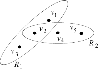
Example 5

Let 𝔸M{\mathbb{A}}_{M} be the algebra introduced in Example 2(3), and RR is the following ternary relation over 𝔸M{\mathbb{A}}_{M} invariant under r,tr,t, given by

R=(001100112201100110220000111102),R=\left(\begin{array}[]{cccccccccc}0&0&1&1&0&0&1&1&2&2\\ 0&1&1&0&0&1&1&0&2&2\\ 0&0&0&0&1&1&1&1&0&2\end{array}\right),

where triples, the elements of the relation are written vertically. Consider the following simple CSP instance from CSP⁡(𝔸M){\rm CSP}({\mathbb{A}}_{M}): 𝒫=(V={v1,v2,v3,v4,v5},{C1=⟨𝐬1=(v1,v2,v3),R1⟩,C2=⟨𝐬2=(v2,v4,v5),R2⟩}𝐶𝐿𝑂𝑆𝐸{\mathcal{P}}=(V=\{v_{1},v_{2},v_{3},v_{4},v_{5}\},\{C^{1}=\langle{\bf s}_{1}=(v_{1},v_{2},v_{3}),R_{1}\rangle,C^{2}=\langle{\bf s}_{2}=(v_{2},v_{4},v_{5}),R_{2}\rangle\}, where R1=R2=RR_{1}=R_{2}=R. To make the instance (2,3)-minimal we run the appropriate local propagation algorithm on it. First, such an algorithm adds new binary constraints Cvi​vj=⟨(vi,vj),Rvi​vj⟩C^{v_{i}v_{j}}=\langle(v_{i},v_{j}),R^{v_{i}v_{j}}\rangle for i,j∈[5]i,j\in[5] starting with Rvi​vj=𝔸M×𝔸MR^{v_{i}v_{j}}={\mathbb{A}}_{M}\times{\mathbb{A}}_{M}. It then iteratively removes pairs from these relations that do not satisfy the (2,3)-minimality condition. Similarly, it tightens the original constraint relations if they violate the conditions of (2,3)-minimality. It is not hard to see that this algorithm does not change constraints C1,C2C^{1},C^{2}, and that the new binary relations are as follows: Rv1​v2=Rv2​v4=Rv1​v4=θR^{v_{1}v_{2}}=R^{v_{2}v_{4}}=R^{v_{1}v_{4}}=\theta, Rv1​v3=Rv2​v3=Rv2​v5=Rv4​v5=QR^{v_{1}v_{3}}=R^{v_{2}v_{3}}=R^{v_{2}v_{5}}=R^{v_{4}v_{5}}=Q, and Rv1​v5=Rv3​v4=Rv3​v5=SR^{v_{1}v_{5}}=R^{v_{3}v_{4}}=R^{v_{3}v_{5}}=S, where

Q=pr13​R\displaystyle Q={\rm pr}_{13}R =\displaystyle= (001122010102),\displaystyle\left(\begin{array}[]{cccccc}0&0&1&1&2&2\\ 0&1&0&1&0&2\end{array}\right),
S\displaystyle S =\displaystyle= (00110220101202).\displaystyle\left(\begin{array}[]{ccccccc}0&0&1&1&0&2&2\\ 0&1&0&1&2&0&2\end{array}\right).

In order to distinguish elements and congruences of domains belonging to different variables let the domain of viv_{i} be denoted by 𝔸i{\mathbb{A}}_{i}, its elements by 0i,1i,2i0_{i},1_{i},2_{i}, and the congruences of 𝔸i{\mathbb{A}}_{i} by 0¯i,θi,1¯i{\underline{0}}_{i},\theta_{i},{\underline{1}}_{i}.

Refer to caption

Figure 4: Instance 𝒫{\mathcal{P}} from Example 5

Let W={v1,v2,v4}W=\{v_{1},v_{2},v_{4}\}, αi=θi\alpha_{i}=\theta_{i} for vi∈Wv_{i}\in W. Then, since Rv1​v2=Rv2​v4=Rv1​v4=θR^{v_{1}v_{2}}=R^{v_{2}v_{4}}=R^{v_{1}v_{4}}=\theta and therefore are αi​αj\alpha_{i}\alpha_{j}-aligned, i,j∈{1,2,4}i,j\in\{1,2,4\}, WW is a strand of 𝒫{\mathcal{P}}. Therefore the instance 𝒫W=({v1,v2,v4},{CW1=⟨(v1,v2),prv1​v2​R1⟩,CW2=⟨(v2,v4),prv2​v4​R2⟩}){\mathcal{P}}_{W}=(\{v_{1},v_{2},v_{4}\},\{C^{1}_{W}=\langle(v_{1},v_{2}),{\rm pr}_{v_{1}v_{2}}R_{1}\rangle,C^{2}_{W}=\langle(v_{2},v_{4}),{\rm pr}_{v_{2}v_{4}}R_{2}\rangle\}) can be decomposed into a disjoint union of two instances

𝒫1\displaystyle{\mathcal{P}}_{1} =\displaystyle= ({v1,v2,v4},{⟨(v1,v2),Q1⟩,⟨(v2,v4),Q2⟩),\displaystyle(\{v_{1},v_{2},v_{4}\},\{\langle(v_{1},v_{2}),Q_{1}\rangle,\langle(v_{2},v_{4}),Q_{2}\rangle),
𝒫2\displaystyle{\mathcal{P}}_{2} =\displaystyle= ({v1,v2,v4},{⟨(v1,v2),S1⟩,⟨(v2,v4),S2⟩),\displaystyle(\{v_{1},v_{2},v_{4}\},\{\langle(v_{1},v_{2}),S_{1}\rangle,\langle(v_{2},v_{4}),S_{2}\rangle),

where Q1={01,11}×{02,12},Q2={02,12}×{04,14}Q_{1}=\{0_{1},1_{1}\}\times\{0_{2},1_{2}\},Q_{2}=\{0_{2},1_{2}\}\times\{0_{4},1_{4}\}, S1={(21,22)},S2={(22,24)}S_{1}=\{(2_{1},2_{2})\},S_{2}=\{(2_{2},2_{4})\}. ⋄\diamond

5.2 Irreducibility

In order to formulate the algorithm properly we need one more transformation of algebras. An algebra 𝔸{\mathbb{A}} is said to be subdirectly irreducible if the intersection of all its nontrivial (different from the equality relation) congruences is nontrivial. This smallest nontrivial congruence μ𝔸\mu_{\mathbb{A}} is called the monolith of 𝔸{\mathbb{A}}, see Fig. 2(b). For instance, the algebra 𝔸M{\mathbb{A}}_{M} from Example 2(3) is subdirectly irreducible, because it has the smallest nontrivial congruence, θ\theta. It is a folklore observation that any CSP instance can be transformed in polynomial time to an instance, in which the domain of every variable is a subdirectly irreducible algebra. We will assume this property of all the instances we consider.

5.3 Block-minimality

Using Lemma 10 we introduce a new type of consistency of a CSP instance, block-minimality, which will be crucial for our algorithm. In a certain sense it is similar to the standard local consistency notions, as it also defined through a family of relations that have to be consistent in a certain way. However, block-minimality is not quite local, and is more difficult to establish, as it involves solving smaller CSP instances recursively. The definitions below are designed to allow for an efficient procedure to establish block-minimality. This is achieved either by allowing for decomposing a subinstance into instances over smaller domains as in Lemma 10, or by replacing large domains with their quotient algebras.

Let αv\alpha_{v} be a congruence of 𝔸v{\mathbb{A}}_{v} for v∈Vv\in V. By 𝒫/α¯{\mathcal{P}}/\lower 2.0pt\hbox{$\scriptstyle\overline{\alpha}$} we denote the instance (V,𝒞α¯)(V,{\mathcal{C}}_{\overline{\alpha}}) constructed as follows: the domain of v∈Vv\in V is 𝔸v/αv{\mathbb{A}}_{v}/\lower 2.0pt\hbox{$\scriptstyle\alpha_{v}$}; for every constraint C=⟨𝐬,R⟩∈𝒞C=\langle{\bf s},R\rangle\in{\mathcal{C}}, 𝐬=(v1,…,vk){\bf s}=(v_{1},\ldots,v_{k}), the set 𝒞α¯{\mathcal{C}}_{\overline{\alpha}} includes the constraint ⟨𝐬,R/α¯⟩\langle{\bf s},R/\lower 2.0pt\hbox{$\scriptstyle\overline{\alpha}$}\rangle, where R/α¯={(𝐚⁡[v1]/αv1,…,𝐚⁡[vk]/αvk)∣𝐚∈R}R/\lower 2.0pt\hbox{$\scriptstyle\overline{\alpha}$}=\{({\bf a}[v_{1}]/\lower 2.0pt\hbox{$\scriptstyle\alpha_{v_{1}}$},\ldots,{\bf a}[v_{k}]/\lower 2.0pt\hbox{$\scriptstyle\alpha_{v_{k}}$})\mid{\bf a}\in R\}.

Example 6

Consider the instance 𝒫{\mathcal{P}} from Example 5, and let αvi=θi\alpha_{v_{i}}=\theta_{i} for each i∈[5]i\in[5]. Then 𝒫/α¯{\mathcal{P}}/\lower 2.0pt\hbox{$\scriptstyle\overline{\alpha}$} is the instance over 𝔸M/θ{\mathbb{A}}_{M}/\lower 2.0pt\hbox{$\scriptstyle\theta$} given by 𝒫/α¯=(V,{⟨𝐬1,R1/α¯⟩,⟨𝐬2,R2/α¯⟩}){\mathcal{P}}/\lower 2.0pt\hbox{$\scriptstyle\overline{\alpha}$}=(V,\{\langle{\bf s}_{1},R_{1}/\lower 2.0pt\hbox{$\scriptstyle\overline{\alpha}$}\rangle,\langle{\bf s}_{2},R_{2}/\lower 2.0pt\hbox{$\scriptstyle\overline{\alpha}$}\rangle\}), where

R1/α¯=R2/α¯=(0/θ2/θ2/θ0/θ2/θ2/θ0/θ0/θ2/θ).R_{1}/\lower 2.0pt\hbox{$\scriptstyle\overline{\alpha}$}=R_{2}/\lower 2.0pt\hbox{$\scriptstyle\overline{\alpha}$}=\left(\begin{array}[]{ccc}0/\lower 2.0pt\hbox{$\scriptstyle\theta$}&2/\lower 2.0pt\hbox{$\scriptstyle\theta$}&2/\lower 2.0pt\hbox{$\scriptstyle\theta$}\\ 0/\lower 2.0pt\hbox{$\scriptstyle\theta$}&2/\lower 2.0pt\hbox{$\scriptstyle\theta$}&2/\lower 2.0pt\hbox{$\scriptstyle\theta$}\\ 0/\lower 2.0pt\hbox{$\scriptstyle\theta$}&0/\lower 2.0pt\hbox{$\scriptstyle\theta$}&2/\lower 2.0pt\hbox{$\scriptstyle\theta$}\end{array}\right).

⋄\diamond

Let 𝒫=(V,𝒞){\mathcal{P}}=(V,{\mathcal{C}}) be a (2,3)-minimal instance, and for X⊆VX\subseteq V, |X|≤2|X|\leq 2, there is a constraint CX=⟨X,RX⟩C^{X}=\langle X,R^{X}\rangle, where RXR^{X} is the set of partial solutions on XX.

Recall that an algebra 𝔸v{\mathbb{A}}_{v} is said to be semilattice free if it does not contain semilattice edges. Let 𝗌𝗂𝗓𝖾⁡(𝒫)\mathsf{size}({\mathcal{P}}) denote the maximal size of domains of 𝒫{\mathcal{P}} that are not semilattice free and 𝖬𝖠𝖷⁡(𝒫)\mathsf{MAX}({\mathcal{P}}) be the set of variables v∈Vv\in V such that |𝔸v|=𝗌𝗂𝗓𝖾⁡(𝒫)|{\mathbb{A}}_{v}|=\mathsf{size}({\mathcal{P}}) and 𝔸v{\mathbb{A}}_{v} is not semilattice free. Finally, for Y⊆VY\subseteq V let μvY=μv\mu^{Y}_{v}=\mu_{v} if v∈Yv\in Y and μvY=0¯v\mu^{Y}_{v}={\underline{0}}_{v} otherwise.

Instance 𝒫{\mathcal{P}} is said to be block-minimal if

  • (BM)

    for every strand U⊆VU\subseteq V the problem 𝒫/U=𝒫/μ¯Y{\mathcal{P}}_{/U}={\mathcal{P}}/\lower 2.0pt\hbox{$\scriptstyle\overline{\mu}^{Y}$}, where Y=𝖬𝖠𝖷⁡(𝒫)−UY=\mathsf{MAX}({\mathcal{P}})-U, is minimal.

The definition of block-minimality is designed in such a way that block-minimality can be efficiently established. Observe that a strand can be large, even equal to VV. However 𝒫/U{\mathcal{P}}_{/U} splits into a union of disjoint problems over smaller domains.

Example 7

Let us consider again the instance 𝒫{\mathcal{P}} from Example 5. In that example we found all its binary solutions, and now we use them to find strands and to verify that this instance is block-minimal. As we saw in Example 5, unless i,j∈{1,2,4}i,j\in\{1,2,4\} the relation Rvi​vjR^{v_{i}v_{j}} is not α​β\alpha\beta-aligned for any congruences α,β\alpha,\beta except the full ones. This means that the only strands of 𝒫{\mathcal{P}} are W={v1,v2,v4}W=\{v_{1},v_{2},v_{4}\} and all the 1-element sets of variables.

Now we check the condition (BM) for 𝒫{\mathcal{P}}. Consider WW. For this strand we have Y={3,5}Y=\{3,5\}, and so μ1Y=μ2Y=μ4Y=0¯\mu^{Y}_{1}=\mu^{Y}_{2}=\mu^{Y}_{4}={\underline{0}} and μ3Y=μ5Y=θ\mu^{Y}_{3}=\mu^{Y}_{5}=\theta. The problem 𝒫/W{\mathcal{P}}_{/W} is the following problem: (V,{C1′,C2′})(V,\{C^{\prime}_{1},C^{\prime}_{2}\}), where C1′=⟨𝐬1,Rθ⟩C^{\prime}_{1}=\langle{\bf s}_{1},R^{\theta}\rangle, C2′=⟨𝐬2,Rθ⟩C^{\prime}_{2}=\langle{\bf s}_{2},R^{\theta}\rangle, and

Rθ=(0011220101220/θ0/θ0/θ0/θ0/θ2/θ).R^{\theta}=\left(\begin{array}[]{cccccc}0&0&1&1&2&2\\ 0&1&0&1&2&2\\ 0/\lower 2.0pt\hbox{$\scriptstyle\theta$}&0/\lower 2.0pt\hbox{$\scriptstyle\theta$}&0/\lower 2.0pt\hbox{$\scriptstyle\theta$}&0/\lower 2.0pt\hbox{$\scriptstyle\theta$}&0/\lower 2.0pt\hbox{$\scriptstyle\theta$}&2/\lower 2.0pt\hbox{$\scriptstyle\theta$}\end{array}\right).

Now, consider first C1C_{1}. For any tuple (a1,a2,a3)∈Rθ(a_{1},a_{2},a_{3})\in R^{\theta}, that is, assignment v1=a1∈𝔸M,v2=a2∈𝔸M,v3=a3∈𝔸M/θv_{1}=a_{1}\in{\mathbb{A}}_{M},v_{2}=a_{2}\in{\mathbb{A}}_{M},v_{3}=a_{3}\in{\mathbb{A}}_{M}/\lower 2.0pt\hbox{$\scriptstyle\theta$}, we can extend this assignment to v4=v2v_{4}=v_{2} and v5=0/θv_{5}=0/\lower 2.0pt\hbox{$\scriptstyle\theta$} to obtain a satisfying assignment of 𝒫/W{\mathcal{P}}_{/W}. For C2C_{2} the argument is the same.

For 1-element strands consider {v2}\{v_{2}\}. Then Y={v1,v3,v4,v5}Y=\{v_{1},v_{3},v_{4},v_{5}\}, and μ1Y=μ3Y=μ4Y=μ5Y=θ\mu^{Y}_{1}=\mu^{Y}_{3}=\mu^{Y}_{4}=\mu^{Y}_{5}=\theta. We have 𝒫/{v2}=(V,{C1′′,C2′′}){\mathcal{P}}_{/\{v_{2}\}}=(V,\{C^{\prime\prime}_{1},C^{\prime\prime}_{2}\}), where C1′′=⟨𝐬1,R1θ​θ⟩C^{\prime\prime}_{1}=\langle{\bf s}_{1},R^{\theta\theta}_{1}\rangle, C2′=⟨𝐬2,R2θ​θ⟩C^{\prime}_{2}=\langle{\bf s}_{2},R^{\theta\theta}_{2}\rangle, and

R1θ​θ=(0/θ0/θ2/θ2/θ01220/θ0/θ0/θ2/θ),R2θ​θ=(01220/θ0/θ2/θ2/θ0/θ0/θ0/θ2/θ).R^{\theta\theta}_{1}=\left(\begin{array}[]{cccc}0/\lower 2.0pt\hbox{$\scriptstyle\theta$}&0/\lower 2.0pt\hbox{$\scriptstyle\theta$}&2/\lower 2.0pt\hbox{$\scriptstyle\theta$}&2/\lower 2.0pt\hbox{$\scriptstyle\theta$}\\ 0&1&2&2\\ 0/\lower 2.0pt\hbox{$\scriptstyle\theta$}&0/\lower 2.0pt\hbox{$\scriptstyle\theta$}&0/\lower 2.0pt\hbox{$\scriptstyle\theta$}&2/\lower 2.0pt\hbox{$\scriptstyle\theta$}\end{array}\right),\qquad R^{\theta\theta}_{2}=\left(\begin{array}[]{cccc}0&1&2&2\\ 0/\lower 2.0pt\hbox{$\scriptstyle\theta$}&0/\lower 2.0pt\hbox{$\scriptstyle\theta$}&2/\lower 2.0pt\hbox{$\scriptstyle\theta$}&2/\lower 2.0pt\hbox{$\scriptstyle\theta$}\\ 0/\lower 2.0pt\hbox{$\scriptstyle\theta$}&0/\lower 2.0pt\hbox{$\scriptstyle\theta$}&0/\lower 2.0pt\hbox{$\scriptstyle\theta$}&2/\lower 2.0pt\hbox{$\scriptstyle\theta$}\end{array}\right).

As is easily seen, any assignment to v1,v2,v3v_{1},v_{2},v_{3} or to v2,v4,v5v_{2},v_{4},v_{5} can be extended to a solution of 𝒫/{v2}{\mathcal{P}}_{/\{v_{2}\}}. ⋄\diamond

For an instance 𝒫{\mathcal{P}} we say that an instance 𝒫′{\mathcal{P}}^{\prime} is strictly smaller than instance 𝒫{\mathcal{P}} if 𝗌𝗂𝗓𝖾⁡(𝒫′)<𝗌𝗂𝗓𝖾⁡(𝒫)\mathsf{size}({\mathcal{P}}^{\prime})<\mathsf{size}({\mathcal{P}}).

Lemma 11

Let 𝒫=(V,𝒞){\mathcal{P}}=(V,{\mathcal{C}}) be a (2,3)-minimal instance. Then 𝒫{\mathcal{P}} can be transformed to an equivalent block-minimal instance 𝒫′{\mathcal{P}}^{\prime} by solving a quadratic number of strictly smaller CSPs.

Proof: To establish block-minimality of 𝒫{\mathcal{P}}, for every strand U⊆VU\subseteq V, we need to check if the problem given in condition (BM) is minimal. If they are then 𝒫{\mathcal{P}} is block-minimal, otherwise some tuples can be removed from some constraint relation RR (the set of tuples that remain in RR is always a subalgebra, as is easily seen), and the instance 𝒫{\mathcal{P}} tightened, in which case we need to repeat the procedure with the tightened instance. Therefore we just need to show how to reduce solving those subproblems to solving strictly smaller CSPs.

By the definition of a strand there is a partition Bw​1,…,Bw​ℓB_{w1},\ldots,B_{w\ell} of 𝔸w{\mathbb{A}}_{w} for w∈Uw\in U such that for every constraint ⟨𝐬,R⟩∈𝒞\langle{\bf s},R\rangle\in{\mathcal{C}}, for any w1,w2∈𝐬∩Uw_{1},w_{2}\in{\bf s}\cap U, any 𝐛∈R{\bf b}\in R, and any i∈[ℓ]i\in[\ell] it holds 𝐛⁡[w1]∈Bw1​i{\bf b}[w_{1}]\in B_{w_{1}i} if and only if 𝐛⁡[w2]∈Bw2​i{\bf b}[w_{2}]\in B_{w_{2}i}. Then the problem 𝒫/U{\mathcal{P}}_{/U} is a disjoint union of instances 𝒫1,…,𝒫ℓ{\mathcal{P}}_{1},\ldots,{\mathcal{P}}_{\ell} given by: 𝒫i=(V,𝒞i){\mathcal{P}}_{i}=(V,{\mathcal{C}}_{i}), where for every constraint C=⟨𝐬,R⟩∈𝒞C=\langle{\bf s},R\rangle\in{\mathcal{C}} there is Ci=⟨𝐬,Ri⟩∈𝒞iC_{i}=\langle{\bf s},R_{i}\rangle\in{\mathcal{C}}_{i} such that

Ri={𝐚′∣𝐚∈R,𝐚[w]∈Bw​i for each w∈𝐬∩U},R_{i}=\{{\bf a}^{\prime}\mid{\bf a}\in R,{\bf a}[w]\in B_{wi}\text{ for each $w\in{\bf s}\cap U$}\},

with 𝐚′​[u]=𝐚⁡[u]/μuY{\bf a}^{\prime}[u]={\bf a}[u]/\lower 2.0pt\hbox{$\scriptstyle\mu^{Y}_{u}$}, Y=𝖬𝖠𝖷⁡(𝒫)−UY=\mathsf{MAX}({\mathcal{P}})-U, for each u∈𝐬u\in{\bf s}. Clearly, 𝗌𝗂𝗓𝖾⁡(𝒫i)<𝗌𝗂𝗓𝖾⁡(𝒫)\mathsf{size}({\mathcal{P}}_{i})<\mathsf{size}({\mathcal{P}}) for each i∈[ℓ]i\in[\ell].

In order to establish the minimality of 𝒫/U{\mathcal{P}}_{/U} it suffices to do the following. Take C=⟨𝐬,R⟩∈𝒞C=\langle{\bf s},R\rangle\in{\mathcal{C}} and 𝐚∈R{\bf a}\in R. We need to check that 𝐚′=𝐚/μ¯Y{\bf a}^{\prime}={\bf a}/\lower 2.0pt\hbox{$\scriptstyle\overline{\mu}^{Y}$}, Y=𝖬𝖠𝖷⁡(𝒫)−UY=\mathsf{MAX}({\mathcal{P}})-U, extends to a solution of at least one of the problems 𝒫1,…,𝒫ℓ{\mathcal{P}}_{1},\ldots,{\mathcal{P}}_{\ell}. For i∈[ℓ]i\in[\ell] let 𝒫i′{\mathcal{P}}_{i}^{\prime} be the problem obtained from 𝒫i{\mathcal{P}}_{i} as follows: fix the values of variables from 𝐬{\bf s} to those of 𝐚′{\bf a}^{\prime}, or in other words, add the constraint ⟨(w),{𝐚⁡[w]/μwY}⟩\langle(w),\{{\bf a}[w]/\lower 2.0pt\hbox{$\scriptstyle\mu^{Y}_{w}$}\}\rangle for each w∈𝐬w\in{\bf s}. Then 𝐚′{\bf a}^{\prime} can be extended to a solution of 𝒫i{\mathcal{P}}_{i} if and only if 𝒫i′{\mathcal{P}}^{\prime}_{i} has a solution. □\Box

5.4 The algorithm

We are now in a position to describe our solution algorithm. In the algorithm we distinguish three cases depending on the presence of semilattice edges and centralizers of the domains of variables. In each case we employ different methods of solving or reducing the instance to a strictly smaller one. Algorithm 1, SolveCSP, gives a more formal description of the solution algorithm.

Let 𝒫=(V,𝒞){\mathcal{P}}=(V,{\mathcal{C}}) be a subdirectly irreducible (2,3)-minimal instance. Let 𝖢𝖾𝗇𝗍𝖾𝗋⁡(𝒫)\mathsf{Center}({\mathcal{P}}) denote the set of variables v∈Vv\in V such that (0¯v:μv)=1¯v({\underline{0}}_{v}:\mu_{v})={\underline{1}}_{v}. Let μv∗=μv\mu^{*}_{v}=\mu_{v} if v∈𝖬𝖠𝖷⁡(𝒫)∩𝖢𝖾𝗇𝗍𝖾𝗋⁡(𝒫)v\in\mathsf{MAX}({\mathcal{P}})\cap\mathsf{Center}({\mathcal{P}}) and μv∗=0¯v\mu^{*}_{v}={\underline{0}}_{v} otherwise.

Semilattice free domains.

If all domains of 𝒫{\mathcal{P}} are semilattice free then 𝒫{\mathcal{P}} can be solved in polynomial time, using the few subpowers algorithm, as shown in [43, 21].

Small centralizers

If μv∗=0¯v\mu^{*}_{v}={\underline{0}}_{v} for all v∈Vv\in V, by Theorem 12 block-minimality guarantees that a solution exists, and we can use Lemma 11 to solve the instance.

Theorem 12

If 𝒫{\mathcal{P}} is subdirectly irreducible, (2,3)-minimal, block-minimal, and 𝖬𝖠𝖷⁡(𝒫)∩𝖢𝖾𝗇𝗍𝖾𝗋⁡(𝒫)=∅\mathsf{MAX}({\mathcal{P}})\cap\mathsf{Center}({\mathcal{P}})=\mathchar 3391\relax, then 𝒫{\mathcal{P}} has a solution.

Large centralizers

Suppose that 𝖬𝖠𝖷⁡(𝒫)∩𝖢𝖾𝗇𝗍𝖾𝗋⁡(𝒫)≠∅\mathsf{MAX}({\mathcal{P}})\cap\mathsf{Center}({\mathcal{P}})\neq\mathchar 3391\relax. In this case the algorithm proceeds in three steps.
Stage 1. Consider the problem 𝒫/μ¯∗{\mathcal{P}}/\lower 2.0pt\hbox{$\scriptstyle\overline{\mu}^{*}$}. We establish the global 1-minimality of this problem. If it is tightened in the process, we start solving the new problem from scratch. To check global 1-minimality, for each v∈Vv\in V and every a∈𝔸v/μv∗a\in{\mathbb{A}}_{v}/\lower 2.0pt\hbox{$\scriptstyle\mu^{*}_{v}$}, we need to find a solution of the instance, or show it does not exists. To this end, add the constraint ⟨(v),{a}⟩\langle(v),\{a\}\rangle to 𝒫/μ¯∗{\mathcal{P}}/\lower 2.0pt\hbox{$\scriptstyle\overline{\mu}^{*}$}. The resulting problem belongs to CSP⁡(𝔸){\rm CSP}({\mathbb{A}}), since 𝔸v{\mathbb{A}}_{v} is idempotent, and hence {a}\{a\} is a subalgebra of 𝔸v/μv∗{\mathbb{A}}_{v}/\lower 2.0pt\hbox{$\scriptstyle\mu^{*}_{v}$}. Then we establish (2,3)-minimality and block minimality of the resulting problem. Let us denote it 𝒫′{\mathcal{P}}^{\prime}. There are two possibilities. First, if 𝗌𝗂𝗓𝖾⁡(𝒫′)<𝗌𝗂𝗓𝖾⁡(𝒫)\mathsf{size}({\mathcal{P}}^{\prime})<\mathsf{size}({\mathcal{P}}) then 𝒫′{\mathcal{P}}^{\prime} is a problem strictly smaller than 𝒫{\mathcal{P}} and can be solved by recursively calling Algorithm 1 on 𝒫′{\mathcal{P}}^{\prime}. If 𝗌𝗂𝗓𝖾⁡(𝒫′)=𝗌𝗂𝗓𝖾⁡(𝒫)\mathsf{size}({\mathcal{P}}^{\prime})=\mathsf{size}({\mathcal{P}}) then, as all the domains 𝔸v{\mathbb{A}}_{v} of maximal size for v∈𝖢𝖾𝗇𝗍𝖾𝗋⁡(𝒫)v\in\mathsf{Center}({\mathcal{P}}) are replaced with their quotient algebras, there is w∉𝖢𝖾𝗇𝗍𝖾𝗋⁡(𝒫)w\not\in\mathsf{Center}({\mathcal{P}}) such that |𝔸w|=𝗌𝗂𝗓𝖾⁡(𝒫)|{\mathbb{A}}_{w}|=\mathsf{size}({\mathcal{P}}) and 𝔸w{\mathbb{A}}_{w} is not semilattice free. Therefore for every u∈𝖢𝖾𝗇𝗍𝖾𝗋⁡(𝒫′)u\in\mathsf{Center}({\mathcal{P}}^{\prime}), for the corresponding domain 𝔸u′{\mathbb{A}}^{\prime}_{u} we have |𝔸u′|<𝗌𝗂𝗓𝖾⁡(𝒫)=𝗌𝗂𝗓𝖾⁡(𝒫′)|{\mathbb{A}}^{\prime}_{u}|<\mathsf{size}({\mathcal{P}})=\mathsf{size}({\mathcal{P}}^{\prime}). Thus, 𝖬𝖠𝖷⁡(𝒫′)∩𝖢𝖾𝗇𝗍𝖾𝗋⁡(𝒫′)=∅\mathsf{MAX}({\mathcal{P}}^{\prime})\cap\mathsf{Center}({\mathcal{P}}^{\prime})=\mathchar 3391\relax, and 𝒫′{\mathcal{P}}^{\prime} has a solution by Theorem 12.
Stage 2. For every v∈𝖬𝖠𝖷⁡(𝒫)v\in\mathsf{MAX}({\mathcal{P}}) we find a solution φ\varphi of 𝒫/μ¯∗{\mathcal{P}}/\lower 2.0pt\hbox{$\scriptstyle\overline{\mu}^{*}$} such that there is a∈𝔸va\in{\mathbb{A}}_{v} such that {a,φ⁡(v)}\{a,\varphi(v)\} is a semilattice edge if μv∗=0¯v\mu^{*}_{v}={\underline{0}}_{v}, or, if μv∗=μv\mu^{*}_{v}=\mu_{v}, there is b∈φ⁡(v)b\in\varphi(v) such that {a,b}\{a,b\} is a semilattice edge. Take v∈𝖬𝖠𝖷⁡(𝒫)v\in\mathsf{MAX}({\mathcal{P}}) and b∈𝔸v/μv∗b\in{\mathbb{A}}_{v}/\lower 2.0pt\hbox{$\scriptstyle\mu^{*}_{v}$} such that {a,b}\{a,b\} is a semilattice edge in 𝔸v/μv∗{\mathbb{A}}_{v}/\lower 2.0pt\hbox{$\scriptstyle\mu^{*}_{v}$} for some a∈𝔸v/μv∗a\in{\mathbb{A}}_{v}/\lower 2.0pt\hbox{$\scriptstyle\mu^{*}_{v}$}. Such a semilattice edge exists, because 𝔸v{\mathbb{A}}_{v} is not semilattice free. Also, if μv∗≠0¯v\mu^{*}_{v}\neq{\underline{0}}_{v}, then v∈𝖢𝖾𝗇𝗍𝖾𝗋⁡(𝒫)v\in\mathsf{Center}({\mathcal{P}}) and (0¯v:μv)=1¯v({\underline{0}}_{v}:\mu_{v})={\underline{1}}_{v} and by Corollary 9 its semilattice edges are all between μv\mu_{v}-blocks. Since 𝒫/μ¯∗{\mathcal{P}}/\lower 2.0pt\hbox{$\scriptstyle\overline{\mu}^{*}$} is globally 1-minimal, there is a solution φv,b\varphi_{v,b} such that φv,b​(v)=b\varphi_{v,b}(v)=b, and therefore φv,b\varphi_{v,b} satisfies the condition. Let 𝖬𝖠𝖷⁡(𝒫)={v1,…,vℓ}\mathsf{MAX}({\mathcal{P}})=\{v_{1},\ldots,v_{\ell}\} and b1,…,bℓb_{1},\ldots,b_{\ell} the values satisfying the requirements above.
Stage 3. We apply the transformation of 𝒫{\mathcal{P}} suggested by Maroti in [55]. For a solution φ\varphi of 𝒫/μ¯∗{\mathcal{P}}/\lower 2.0pt\hbox{$\scriptstyle\overline{\mu}^{*}$}, by 𝒫⋅φ{\mathcal{P}}\cdot\varphi we denote the instance (V,𝒞φ)(V,{\mathcal{C}}_{\varphi}) given by the rule: for every C=⟨𝐬,R⟩∈𝒞C=\langle{\bf s},R\rangle\in{\mathcal{C}} the set 𝒞φ{\mathcal{C}}_{\varphi} contains a constraint ⟨𝐬,R⋅φ⟩\langle{\bf s},R\cdot\varphi\rangle. To construct R⋅φR\cdot\varphi choose a tuple 𝐛∈R{\bf b}\in R such that 𝐛⁡[v]/μv∗=φ⁡(v){\bf b}[v]/\lower 2.0pt\hbox{$\scriptstyle\mu^{*}_{v}$}=\varphi(v) for all v∈𝐬v\in{\bf s}; this is possible because φ\varphi is a solution of 𝒫/μ¯∗{\mathcal{P}}/\lower 2.0pt\hbox{$\scriptstyle\overline{\mu}^{*}$}. Then set R⋅φ={𝐚⋅𝐛∣𝐚∈R}R\cdot\varphi=\{{\bf a}\cdot{\bf b}\mid{\bf a}\in R\}. By the results of [55] and Lemma 8 the instance 𝒫⋅φ{\mathcal{P}}\cdot\varphi has a solution if and only if 𝒫{\mathcal{P}} does. We now use the solutions φv1,b1,…,φvℓ,bℓ\varphi_{v_{1},b_{1}},\ldots,\varphi_{v_{\ell},b_{\ell}} to construct a new problem

𝒫1=(…​((𝒫⋅φv1,b1)⋅φv2,b2)⋅…)⋅φvℓ,bℓ.{\mathcal{P}}^{1}=(\dots(({\mathcal{P}}\cdot\varphi_{v_{1},b_{1}})\cdot\varphi_{v_{2},b_{2}})\cdot\dots)\cdot\varphi_{v_{\ell},b_{\ell}}.

Note that the transformation of 𝒫{\mathcal{P}} above boils down to a collection of mappings pv:𝔸v→𝔸vp_{v}:{\mathbb{A}}_{v}\to{\mathbb{A}}_{v}, v∈Vv\in V, so called consistent mappings, see Section 5.5, that also satisfy some additional properties. If we now repeat the procedure above starting from 𝒫1{\mathcal{P}}^{1} and using the same solutions φvi,bi\varphi_{v_{i},b_{i}}, we obtain an instance 𝒫2{\mathcal{P}}^{2}, for which the corresponding collection of consistent mappings is pv∘pvp_{v}\circ p_{v}, v∈Vv\in V. More generally,

𝒫i+1=(…​((𝒫i⋅φv1,b1)⋅φv2,b2)⋅…)⋅φvℓ,bℓ.{\mathcal{P}}^{i+1}=(\dots(({\mathcal{P}}^{i}\cdot\varphi_{v_{1},b_{1}})\cdot\varphi_{v_{2},b_{2}})\cdot\dots)\cdot\varphi_{v_{\ell},b_{\ell}}.

There is kk such that pvkp^{k}_{v} is idempotent for every v∈Vv\in V, that is, (pvk∘pvk)​(x)=pvk​(x)(p^{k}_{v}\circ p^{k}_{v})(x)=p^{k}_{v}(x) for all xx. Set 𝒫†=𝒫k{\mathcal{P}}^{\dagger}={\mathcal{P}}^{k}. We will show later that 𝗌𝗂𝗓𝖾⁡(𝒫†)<𝗌𝗂𝗓𝖾⁡(𝒫)\mathsf{size}({\mathcal{P}}^{\dagger})<\mathsf{size}({\mathcal{P}}).

This last case can be summarized as the following

Theorem 13

If 𝒫/μ¯∗{\mathcal{P}}/\lower 2.0pt\hbox{$\scriptstyle\overline{\mu}^{*}$} is globally 1-minimal, then 𝒫{\mathcal{P}} can be reduced in polynomial time to a strictly smaller instance over a class of algebras satisfying the conditions of the Dichotomy Conjecture.

Algorithm 1 Procedure SolveCSP
0:  A CSP instance 𝒫=(V,𝒞){\mathcal{P}}=(V,{\mathcal{C}}) over 𝒜{\mathcal{A}}
0:  A solution of 𝒫{\mathcal{P}} if one exists, ‘NO’ otherwise
1:  if all the domains are semilattice free then
2:   Solve 𝒫{\mathcal{P}} using the few subpowers algorithm and RETURN the answer
3:  end if
4:  Transform 𝒫{\mathcal{P}} to a subdirectly irreducible, block-minimal and (2,3)-minimal instance
5:  μv∗=μv\mu^{*}_{v}=\mu_{v} for v∈𝖬𝖠𝖷⁡(𝒫)∩𝖢𝖾𝗇𝗍𝖾𝗋⁡(𝒫)v\in\mathsf{MAX}({\mathcal{P}})\cap\mathsf{Center}({\mathcal{P}}) and μv∗=0¯v\mu^{*}_{v}={\underline{0}}_{v} otherwise
6:  𝒫∗=𝒫/μ¯∗{\mathcal{P}}^{*}={\mathcal{P}}/\lower 2.0pt\hbox{$\scriptstyle\overline{\mu}^{*}$}
7:  /* the global 1-minimality of 𝒫∗{\mathcal{P}}^{*}
8:  for every v∈Vv\in V and a∈𝔸v/μv∗a\in{\mathbb{A}}_{v}/\lower 2.0pt\hbox{$\scriptstyle\mu^{*}_{v}$} do
9:   𝒫′=𝒫(v,a)∗{\mathcal{P}}^{\prime}={\mathcal{P}}^{*}_{(v,a)} /* Add constraint ⟨(v),{a}⟩\langle(v),\{a\}\rangle fixing the value of vv to aa
10:   Transform 𝒫′{\mathcal{P}}^{\prime} to a subdirectly irreducible, (2,3)-minimal instance 𝒫′′{\mathcal{P}}^{\prime\prime}
11:   If 𝗌𝗂𝗓𝖾⁡(𝒫′′)<𝗌𝗂𝗓𝖾⁡(𝒫)\mathsf{size}({\mathcal{P}}^{\prime\prime})<\mathsf{size}({\mathcal{P}}) call SolveCSP on 𝒫′′{\mathcal{P}}^{\prime\prime} and flag aa if 𝒫′′{\mathcal{P}}^{\prime\prime} has no solution
12:   Establish block-minimality of 𝒫′′{\mathcal{P}}^{\prime\prime}; if the problem changes, return to Step 10
13:   If the resulting instance is empty, flag the element aa
14:  end for
15:  If there are flagged values, tighten the instance by removing the flagged elements and start over
16:  Use Theorem 13 to reduce 𝒫{\mathcal{P}} to an instance 𝒫†{\mathcal{P}}^{\dagger} with 𝗌𝗂𝗓𝖾⁡(𝒫†)<𝗌𝗂𝗓𝖾⁡(𝒫)\mathsf{size}({\mathcal{P}}^{\dagger})<\mathsf{size}({\mathcal{P}})
17:  Call SolveCSP on 𝒫†{\mathcal{P}}^{\dagger} and RETURN the answer

We now illustrate the algorithm on our running example.

Example 8

We illustrate the algorithm SolveCSP on the instance from Example 5. Recall that the domain of each variable is 𝔸M{\mathbb{A}}_{M}, its monolith is θ\theta, and (0¯:θ)({\underline{0}}:\theta) is the full relation. This means that 𝗌𝗂𝗓𝖾⁡(𝒫)=3\mathsf{size}({\mathcal{P}})=3, 𝖬𝖠𝖷⁡(𝒫)=V\mathsf{MAX}({\mathcal{P}})=V and 𝖢𝖾𝗇𝗍𝖾𝗋⁡(𝒫)=V\mathsf{Center}({\mathcal{P}})=V, as well. Therefore we are in the case of large centralizers. Set μvi∗=θi\mu^{*}_{v_{i}}=\theta_{i} for each i∈[5]i\in[5] and consider the problem 𝒫/μ¯∗=(V,{C1∗=⟨𝐬1,R1∗⟩,C2∗=⟨𝐬2,R2∗⟩){\mathcal{P}}/\lower 2.0pt\hbox{$\scriptstyle\overline{\mu}*$}=(V,\{C^{*}_{1}=\langle{\bf s}_{1},R^{*}_{1}\rangle,C^{*}_{2}=\langle{\bf s}_{2},R^{*}_{2}\rangle), where

R∗=(0/θ2/θ2/θ0/θ2/θ2/θ0/θ0/θ2/θ).R^{*}=\left(\begin{array}[]{ccc}0/\lower 2.0pt\hbox{$\scriptstyle\theta$}&2/\lower 2.0pt\hbox{$\scriptstyle\theta$}&2/\lower 2.0pt\hbox{$\scriptstyle\theta$}\\ 0/\lower 2.0pt\hbox{$\scriptstyle\theta$}&2/\lower 2.0pt\hbox{$\scriptstyle\theta$}&2/\lower 2.0pt\hbox{$\scriptstyle\theta$}\\ 0/\lower 2.0pt\hbox{$\scriptstyle\theta$}&0/\lower 2.0pt\hbox{$\scriptstyle\theta$}&2/\lower 2.0pt\hbox{$\scriptstyle\theta$}\end{array}\right).

It is an easy exercise to show that this instance is globally 1-minimal (every value 0/θ0/\lower 2.0pt\hbox{$\scriptstyle\theta$} can be extended to the all-0/θ0/\lower 2.0pt\hbox{$\scriptstyle\theta$} solution, and every value 2/θ2/\lower 2.0pt\hbox{$\scriptstyle\theta$} can be extended to the all-2/θ2/\lower 2.0pt\hbox{$\scriptstyle\theta$} solution). This completes Stage 1. For every variable viv_{i} we choose b∈𝔸M/θb\in{\mathbb{A}}_{M}/\lower 2.0pt\hbox{$\scriptstyle\theta$} such that for some a∈𝔸M/θa\in{\mathbb{A}}_{M}/\lower 2.0pt\hbox{$\scriptstyle\theta$} the pair {a,b}\{a,b\} is a semilattice edge. Since 𝔸M/θ{\mathbb{A}}_{M}/\lower 2.0pt\hbox{$\scriptstyle\theta$} is a 2-element semilattice, setting b=0/θb=0/\lower 2.0pt\hbox{$\scriptstyle\theta$} and a=2/θa=2/\lower 2.0pt\hbox{$\scriptstyle\theta$} is the only choice. Therefore φvi,bi\varphi_{v_{i},b_{i}} in our case can be chosen to be the same solution φ\varphi given by φ⁡(vi)=0/θ\varphi(v_{i})=0/\lower 2.0pt\hbox{$\scriptstyle\theta$}; and Stage 2 is completed. For Stage 3 first note that in 𝔸M{\mathbb{A}}_{M} the operation rr plays the role of multiplication ⋅\cdot. Then for each of the constraints C1,C2C^{1},C^{2} choose a representative 𝐚1∈R1∩(φ⁡(v1)×φ⁡(v2)×φ⁡(v3))=R1∩{0,1}3{\bf a}_{1}\in R_{1}\cap(\varphi(v_{1})\times\varphi(v_{2})\times\varphi(v_{3}))=R_{1}\cap\{0,1\}^{3}, 𝐚2∈R2∩(φ⁡(v2)×φ⁡(v4)×φ⁡(v5))=R2∩{0,1}3{\bf a}_{2}\in R_{2}\cap(\varphi(v_{2})\times\varphi(v_{4})\times\varphi(v_{5}))=R_{2}\cap\{0,1\}^{3}, and set 𝒫′=({v1,…,v5},{C1′=⟨(v1,v2,v3),R1′⟩,C2′=⟨(v2,v4,v5),R2′⟩}){\mathcal{P}}^{\prime}=(\{v_{1},\ldots,v_{5}\},\{C^{\prime}_{1}=\langle(v_{1},v_{2},v_{3}),R^{\prime}_{1}\rangle,C^{\prime}_{2}=\langle(v_{2},v_{4},v_{5}),R^{\prime}_{2}\rangle\}), where R1′=r⁡(R1,𝐚)R^{\prime}_{1}=r(R_{1},{\bf a}), R2′=r⁡(R2,𝐛)R^{\prime}_{2}=r(R_{2},{\bf b}). Since r⁡(2,0)=r⁡(2,1)=0r(2,0)=r(2,1)=0, regardless of the choice of 𝐚,𝐛{\bf a},{\bf b} in our case R1′⊆R1,R2′⊆R2R^{\prime}_{1}\subseteq R_{1},R^{\prime}_{2}\subseteq R_{2}, and are invariant with respect to the affine operation of ℤ2{\mathbb{Z}}_{2}. Therefore the instance 𝒫′{\mathcal{P}}^{\prime} can be viewed as a system of linear equations over ℤ2{\mathbb{Z}}_{2} (this system is actually empty in our case), and can be easily solved. ⋄\diamond

Using Lemma 11 and Theorems 12,13 it is not difficult to see that the algorithm runs in polynomial time.

Theorem 14

Algorithm SolveCSP (Algorithm 1) correctly solves every instance from CSP⁡(𝒜){\rm CSP}({\mathcal{A}}) and runs in polynomial time.

Proof: By the results of [21, 25] the algorithm correctly solves the given instance 𝒫{\mathcal{P}} in polynomial time if the conditions of Step 1 are true. Lemma 11 implies that Steps 4 and 12 can be completed by recursing to strictly smaller instances.

Next we show that the for-loop in Steps 8-14 checks if 𝒫∗=𝒫/μ¯∗{\mathcal{P}}^{*}={\mathcal{P}}/\lower 2.0pt\hbox{$\scriptstyle\overline{\mu}^{*}$} is globally 1-minimal. For this we need to verify that a value aa is flagged if and only if 𝒫∗{\mathcal{P}}^{*} has no solution φ\varphi with φ⁡(v)=a\varphi(v)=a, and therefore if no values are flagged then 𝒫∗{\mathcal{P}}^{*} is globally 1-minimal. If φ⁡(v)=a\varphi(v)=a for some solution φ\varphi of 𝒫∗{\mathcal{P}}^{*}, then φ\varphi is a solution 𝒫′{\mathcal{P}}^{\prime} constructed in Step 9. In this case Steps 11,12 cannot result in an empty instance. Suppose a∈𝔸v/μv∗a\in{\mathbb{A}}_{v}/\lower 2.0pt\hbox{$\scriptstyle\mu^{*}_{v}$} is not flagged. If 𝗌𝗂𝗓𝖾⁡(𝒫′′)<𝗌𝗂𝗓𝖾⁡(𝒫)\mathsf{size}({\mathcal{P}}^{\prime\prime})<\mathsf{size}({\mathcal{P}}) this means that 𝒫′′{\mathcal{P}}^{\prime\prime} and therefore 𝒫′{\mathcal{P}}^{\prime} has a solution. Otherwise this means that establishing block-minimality of 𝒫′′{\mathcal{P}}^{\prime\prime} is successful. In this case 𝒫′′{\mathcal{P}}^{\prime\prime} has a solution by Theorem 12, because 𝖬𝖠𝖷⁡(𝒫′′)∩𝖢𝖾𝗇𝗍𝖾𝗋⁡(𝒫′′)=∅\mathsf{MAX}({\mathcal{P}}^{\prime\prime})\cap\mathsf{Center}({\mathcal{P}}^{\prime\prime})=\mathchar 3391\relax. This in turn implies that 𝒫′{\mathcal{P}}^{\prime} has a solution. Observe also that the set of unflagged values for each variable v∈Vv\in V is a subalgebra of 𝔸/μ∗{\mathbb{A}}/\lower 2.0pt\hbox{$\scriptstyle\mu^{*}$}. Indeed, the set of solutions of 𝒫∗{\mathcal{P}}^{*} is a subalgebra 𝒮∗{\mathcal{S}}^{*} of ∏v∈V𝔸/μ∗\prod_{v\in V}{\mathbb{A}}/\lower 2.0pt\hbox{$\scriptstyle\mu^{*}$}, and the set of unflagged values is the projection of 𝒮∗{\mathcal{S}}^{*} on the coordinate position vv.

Finally, if Steps 8–15 are completed without restarts, Steps 16,17 can be completed by Theorem 13, and recursing on 𝒫′{\mathcal{P}}^{\prime} such that either 𝗌𝗂𝗓𝖾⁡(𝒫′)<𝗌𝗂𝗓𝖾⁡(𝒫)\mathsf{size}({\mathcal{P}}^{\prime})<\mathsf{size}({\mathcal{P}}) or 𝖬𝖠𝖷⁡(𝒫′)∩𝖢𝖾𝗇𝗍𝖾𝗋⁡(𝒫′)=∅\mathsf{MAX}({\mathcal{P}}^{\prime})\cap\mathsf{Center}({\mathcal{P}}^{\prime})=\mathchar 3391\relax.

To see that the algorithm runs in polynomial time it suffices to observe that
(1) The number of restarts in Steps 4 and 15 is at most linear, as the instance becomes smaller after every restart; therefore the number of times Steps 4–15 are executed together is at most linear.
(2) The number of iterations of the for-loop in Steps 8–14 is linear.
(3) The number of restarts in Steps 10 and 12 is at most linear, as the instance becomes smaller after every iteration.
(4) Every call of SolveCSP when establishing block-minimality in Steps 4, and 12 is made on an instance strictly smaller than 𝒫{\mathcal{P}}, and therefore the depth of recursion is bounded by 𝗌𝗂𝗓𝖾⁡(𝒫)\mathsf{size}({\mathcal{P}}) in Step 4,11,12 and 17.
Thus a more thorough estimation gives a bound on the running time of O⁡(n3​k)O(n^{3k}), where kk is the maximal size of an algebra in 𝒜{\mathcal{A}}. □\Box

5.5 Proof of Theorem 13

Following [55] let 𝒫=(V,𝒞){\mathcal{P}}=(V,{\mathcal{C}}) be an instance and pv:𝔸v→𝔸vp_{v}\colon{\mathbb{A}}_{v}\to{\mathbb{A}}_{v}, v∈Vv\in V. Mappings pvp_{v}, v∈Vv\in V, are said to be consistent if for any ⟨𝐬,R⟩∈𝒞\langle{\bf s},R\rangle\in{\mathcal{C}}, 𝐬=(v1,…,vk){\bf s}=(v_{1},\ldots,v_{k}), and any tuple 𝐚∈R{\bf a}\in R the tuple (pv1​(𝐚⁡[1]),…,pvk​(𝐚⁡[k]))(p_{v_{1}}({\bf a}[1]),\ldots,p_{v_{k}}({\bf a}[k])) belongs to RR. It is easy to see that the composition of two families of consistent mappings is also a consistent mapping. For consistent idempotent mappings pvp_{v} by p⁡(𝒫)p({\mathcal{P}}) we denote the retraction of 𝒫{\mathcal{P}}, that is, 𝒫{\mathcal{P}} restricted to the images of pvp_{v}. In this case 𝒫{\mathcal{P}} has a solution if and only if p⁡(𝒫)p({\mathcal{P}}) has, see [55].

Let φ\varphi be a solution of 𝒫/μ¯∗{\mathcal{P}}/\lower 2.0pt\hbox{$\scriptstyle\overline{\mu}^{*}$}. We define pvφ:𝔸v→𝔸vp^{\varphi}_{v}:{\mathbb{A}}_{v}\to{\mathbb{A}}_{v} as follows: pvφ=qvkp^{\varphi}_{v}=q_{v}^{k}, where qv​(a)=a⋅bvq_{v}(a)=a\cdot b_{v}, element bvb_{v} is any element of φ⁡(v)\varphi(v), and kk is such that qvkq_{v}^{k} is idempotent for all v∈Vv\in V. Note that by Lemma 8 this mapping is properly defined even if μv∗≠0¯v\mu^{*}_{v}\neq{\underline{0}}_{v}.

Lemma 15

Mappings pvφp^{\varphi}_{v}, v∈Vv\in V, are consistent.

Proof: Take any C=⟨𝐬,R⟩∈𝒞C=\langle{\bf s},R\rangle\in{\mathcal{C}}. Since φ\varphi is a solution of 𝒫/μ¯∗{\mathcal{P}}/\lower 2.0pt\hbox{$\scriptstyle\overline{\mu}^{*}$}, there is 𝐛∈R{\bf b}\in R such that 𝐛⁡[v]∈φ⁡(v){\bf b}[v]\in\varphi(v) for v∈𝐬v\in{\bf s}. Then for any 𝐚∈R{\bf a}\in R, q⁡(𝐚)=𝐚⋅𝐛∈Rq({\bf a})={\bf a}\cdot{\bf b}\in R, and this product does not depend on the choice of 𝐛{\bf b}, as it follows from Lemma 8. Iterating this operation also produces a tuple from RR. □\Box

We are now in a position to prove Theorem 13.

Proof:[of Theorem 13] We need to show 3 properties of the problem 𝒫†{\mathcal{P}}^{\dagger} constructed in Stage 3: (a) 𝒫{\mathcal{P}} has a solution if and only if 𝒫†{\mathcal{P}}^{\dagger} does; (b) for every v∈𝖬𝖠𝖷⁡(𝒫)v\in\mathsf{MAX}({\mathcal{P}}), |𝔸v†|<|𝔸v||{\mathbb{A}}^{\dagger}_{v}|<|{\mathbb{A}}_{v}|, where 𝔸v†{\mathbb{A}}^{\dagger}_{v} is the domain of vv in 𝒫†{\mathcal{P}}^{\dagger}; and (c) every algebra 𝔸v†{\mathbb{A}}^{\dagger}_{v} has a weak near-unanimity term operation. We use the inductive definition of 𝒫†{\mathcal{P}}^{\dagger} given in Stage 3.

Recall that 𝖬𝖠𝖷⁡(𝒫)={v1,…,vℓ}\mathsf{MAX}({\mathcal{P}})=\{v_{1},\ldots,v_{\ell}\}, ai,bi∈𝔸via_{i},b_{i}\in{\mathbb{A}}_{v_{i}} are such that ai≤bia_{i}\leq b_{i} and bi∈φvi,bi​(vi)b_{i}\in\varphi_{v_{i},b_{i}}(v_{i}), where φvi,bi\varphi_{v_{i},b_{i}} is a solution of 𝒫/μ¯∗{\mathcal{P}}/\lower 2.0pt\hbox{$\scriptstyle\overline{\mu}^{*}$}. For v∈Vv\in V let mapping pv​i:𝔸v→𝔸vp_{vi}:{\mathbb{A}}_{v}\to{\mathbb{A}}_{v} be given by

pv​i​(x)=(…​(x⋅φv1,b1​(v))⋅…)⋅φvi,bi​(v),p_{vi}(x)=(\dots(x\cdot\varphi_{v_{1},b_{1}}(v))\cdot\dots)\cdot\varphi_{v_{i},b_{i}}(v),

where if μv∗=μv\mu^{*}_{v}=\mu_{v} by Lemma 8 the multiplication by φvj,bj​(v)\varphi_{v_{j},b_{j}}(v) does not depend on the choice of a representative from φvj,bj​(v)\varphi_{v_{j},b_{j}}(v). By Lemma 15 {pv​i}\{p_{vi}\} for every ii, and so {pv}\{p_{v}\} and {pvk}\{p^{k}_{v}\} are collections of consistent mappings. Now (a) follows from [55].

Next we show that for every j≤i≤ℓj\leq i\leq\ell it holds that |pv​i​(𝔸vj)|<|𝔸vj||p_{vi}({\mathbb{A}}_{v_{j}})|<|{\mathbb{A}}_{v_{j}}|. Since applying mappings to a set does not increase its cardinality, this implies (b). If |pv​j−1​(𝔸vj)|<|𝔸vj||p_{vj-1}({\mathbb{A}}_{v_{j}})|<|{\mathbb{A}}_{v_{j}}|, we have the desired inequality applying the observation in the previous sentence. Otherwise aj∈𝔸vj=pv​j−1​(𝔸vj)a_{j}\in{\mathbb{A}}_{v_{j}}=p_{vj-1}({\mathbb{A}}_{v_{j}}), and it suffices to notice that aj⋅φvj,bj​(vj)=bj⋅φvj,bj​(vj)=bja_{j}\cdot\varphi_{v_{j},b_{j}}(v_{j})=b_{j}\cdot\varphi_{v_{j},b_{j}}(v_{j})=b_{j}.

To prove (c) observe that if 𝔸v{\mathbb{A}}_{v} is semilattice free then pvφp^{\varphi}_{v} is the identity mapping for any φ\varphi by Lemma 7, and so 𝔸v†=𝔸v{\mathbb{A}}^{\dagger}_{v}={\mathbb{A}}_{v}. For the remaining domains let ff be a weak near-unanimity term of the class 𝒜{\mathcal{A}}. Then for any idempotent mapping pp the operation p∘fp\circ f given by (p∘f)​(x1,…,xn)=p⁡(f⁡(x1,…,xn))(p\circ f)(x_{1},\ldots,x_{n})=p(f(x_{1},\ldots,x_{n})) is a weak near-unanimity term of p⁡(𝒜)={p⁡(𝔸)∣𝔸∈𝒜}p({\mathcal{A}})=\{p({\mathbb{A}})\mid{\mathbb{A}}\in{\mathcal{A}}\}. The result follows. □\Box

6 Algebra technicalities

The rest of the paper is dedicated to proving Theorem 12. This part assumes some familiarity with algebraic terminology. A brief review of the necessary facts from universal algebra can be found in [26]. In this section we remind some results from [26] necessary for our proof.

6.1 Coloured graphs

In [16, 30] we introduced a local approach to the structure of finite algebras. As we use this approach in the proof of Theorem 12, we present the necessary elements of it here, see also [23, 24]. For the sake of the definitions below we slightly abuse terminology and by a module mean the full idempotent reduct of a module.

For an algebra 𝔸{\mathbb{A}} the graph 𝒢⁡(𝔸){\mathcal{G}}({\mathbb{A}}) is defined as follows. The vertex set is the universe AA of 𝔸{\mathbb{A}}. A pair a​bab of vertices is an edge if and only if there exists a maximal congruence θ\theta of 𝖲𝗀⁡(a,b){\sf Sg}(a,b), and a term operation ff of 𝔸{\mathbb{A}} such that either 𝖲𝗀⁡(a,b)/θ{\sf Sg}(a,b)/\lower 2.0pt\hbox{$\scriptstyle\theta$} is a module and ff is an affine operation on it, or ff is a semilattice operation on {a/θ,b/θ}\{a/\lower 2.0pt\hbox{$\scriptstyle\theta$},b/\lower 2.0pt\hbox{$\scriptstyle\theta$}\}, or ff is a majority operation on {a/θ,b/θ}\{a/\lower 2.0pt\hbox{$\scriptstyle\theta$},b/\lower 2.0pt\hbox{$\scriptstyle\theta$}\}. (Note that we use the same operation symbol in this case.) If there are a maximal congruence θ\theta and a term operation ff of 𝔸{\mathbb{A}} such that ff is a semilattice operation on {a/θ,b/θ}\{a/\lower 2.0pt\hbox{$\scriptstyle\theta$},b/\lower 2.0pt\hbox{$\scriptstyle\theta$}\} then a​bab is said to have the semilattice type. An edge a​bab is of majority type if there are a maximal congruence θ\theta and a term operation ff such that ff is a majority operation on {a/θ,b/θ}\{a/\lower 2.0pt\hbox{$\scriptstyle\theta$},b/\lower 2.0pt\hbox{$\scriptstyle\theta$}\} and there is no semilattice term operation on {a/θ,b/θ}\{a/\lower 2.0pt\hbox{$\scriptstyle\theta$},b/\lower 2.0pt\hbox{$\scriptstyle\theta$}\}. Finally, a​bab has the affine type if there are θ\theta and ff such that ff is an affine operation on 𝖲𝗀⁡(a,b)/θ{\sf Sg}(a,b)/\lower 2.0pt\hbox{$\scriptstyle\theta$} and 𝖲𝗀⁡(a,b)/θ{\sf Sg}(a,b)/\lower 2.0pt\hbox{$\scriptstyle\theta$} is a module. Pairs of the form {a/θ,b/θ}\{a/\lower 2.0pt\hbox{$\scriptstyle\theta$},b/\lower 2.0pt\hbox{$\scriptstyle\theta$}\} will be referred to as thick edges.

Properties of 𝒢⁡(𝔸){\mathcal{G}}({\mathbb{A}}) are related to the properties of the algebra 𝔸{\mathbb{A}}.

Theorem 16 (Theorem 5 of [23])

Let 𝔸{\mathbb{A}} be an idempotent algebra 𝔸{\mathbb{A}} such that 𝗏𝖺𝗋⁡(𝔸){\sf var}({\mathbb{A}}) omits type 1. Then

  • (1)

    any two elements of 𝔸{\mathbb{A}} are connected by a sequence of edges of the semilattice, majority, and affine types;

  • (2)

    𝗏𝖺𝗋⁡(𝔸){\sf var}({\mathbb{A}}) omits types 1 and 2 if and only if 𝒢⁡(𝔸){\mathcal{G}}({\mathbb{A}}) satisfies the conditions of item (1) and contains no edges of the affine type.

We use the following refinement of this construction. Let 𝒜{\mathcal{A}} be a finite class of finite smooth algebras. A ternary term operation g′g^{\prime} of 𝒜{\mathcal{A}} is said to satisfy the majority condition for 𝒜{\mathcal{A}} if g′g^{\prime} is a majority operation on every thick majority edge of every algebra from 𝒜{\mathcal{A}}. A ternary term operation h′h^{\prime} is said to satisfy the minority condition for 𝒜{\mathcal{A}} if h′h^{\prime} is a Mal’tsev operation on every thick affine edge. Operations satisfying the majority and minority conditions always exists, as is proved in [23, Theorem 21]. Fix an operation hh satisfying the minority condition, it can also be chosen to satisfy the equation h⁡(h⁡(x,y,y),y,y)=h⁡(x,y,y)h(h(x,y,y),y,y)=h(x,y,y). A pair of elements a,b∈𝔸∈𝒜a,b\in{\mathbb{A}}\in{\mathcal{A}} is said to be

  • (1)

    a semilattice edge if there is a term operation ff such that f⁡(a,b)=f⁡(b,a)=bf(a,b)=f(b,a)=b;

  • (2)

    a thin majority edge if for any term operation g′g^{\prime} satisfying the majority condition the subalgebras 𝖲𝗀⁡(a,g′​(a,b,b)),𝖲𝗀⁡(a,g′​(b,a,b)),𝖲𝗀⁡(a,g′​(b,b,a)){\sf Sg}(a,g^{\prime}(a,b,b)),{\sf Sg}(a,g^{\prime}(b,a,b)),{\sf Sg}(a,g^{\prime}(b,b,a)) contain bb.

  • (3)

    a thin affine edge if h⁡(b,a,a)=bh(b,a,a)=b and b∈𝖲𝗀⁡(a,h′​(a,a,b))b\in{\sf Sg}(a,h^{\prime}(a,a,b)) for any term operation h′h^{\prime} satisfying the minority condition.

Note that thin edges are directed, as aa and bb appear asymmetrically. By 𝒢′​(𝔸){\mathcal{G}}^{\prime}({\mathbb{A}}) we denote the graph whose vertices are the elements of 𝔸{\mathbb{A}}, and the edges are the thin edges defined above. Theorem 21 from [23] also implies that there exists a binary term operation ⋅\cdot of 𝔸{\mathbb{A}} that is a semilattice operation on every thin semilattice edge.

We distinguish several types of paths in 𝒢′​(𝔸){\mathcal{G}}^{\prime}({\mathbb{A}}) depending on the types of edges involved. A directed path in 𝒢′​(𝔸){\mathcal{G}}^{\prime}({\mathbb{A}}) is called an asm-path, if there is an asm-path from aa to bb we write a⊑a​s​mba\sqsubseteq_{asm}b. If all edges of this path are semilattice or affine, it is called an affine-semilattice path or an as-path, if there is an as-path from aa to bb we write a⊑a​sba\sqsubseteq_{as}b. We consider strongly connected components of 𝒢′​(𝔸){\mathcal{G}}^{\prime}({\mathbb{A}}) with majority edges removed, and the natural partial order on such components. The maximal components will be called as-components, and the elements from as-components are called as-maximal; the set of all as-maximal elements of 𝔸{\mathbb{A}} is denoted by 𝖺𝗆𝖺𝗑⁡(𝔸)\mathsf{amax}({\mathbb{A}}). An alternative way to define as-maximal elements is as follows: aa is as-maximal if for every b∈𝔸b\in{\mathbb{A}} such that a⊑a​sba\sqsubseteq_{as}b it also holds that b⊑a​sab\sqsubseteq_{as}a. Finally, element a∈𝔸a\in{\mathbb{A}} is said to be universally maximal (or u-maximal for short) if for every b∈𝔸b\in{\mathbb{A}} such that a⊑a​s​mba\sqsubseteq_{asm}b it also holds that b⊑a​s​mab\sqsubseteq_{asm}a. The set of all u-maximal elements of 𝔸{\mathbb{A}} is denoted 𝗎𝗆𝖺𝗑⁡(𝔸)\mathsf{umax}({\mathbb{A}}).

U-maximality has additional useful properties.

Lemma 17 (Theorem 23, [24]; Lemma 12, [26])

(1) Any two u-maximal elements are connected with an asm-path,
(2) Let 𝔹{\mathbb{B}} be a subalgebra of 𝔸{\mathbb{A}} containing a u-maximal element of 𝔸{\mathbb{A}}. Then every element u-maximal in 𝔹{\mathbb{B}} is also u-maximal in 𝔸{\mathbb{A}}. In particular, if α\alpha is a congruence of 𝔸{\mathbb{A}} and 𝔹{\mathbb{B}} is a u-maximal α\alpha-block, that is 𝔹{\mathbb{B}} is a u-maximal element in 𝔸/α{\mathbb{A}}/\lower 2.0pt\hbox{$\scriptstyle\alpha$}, then 𝗎𝗆𝖺𝗑⁡(𝔹)⊆𝗎𝗆𝖺𝗑⁡(𝔸)\mathsf{umax}({\mathbb{B}})\subseteq\mathsf{umax}({\mathbb{A}}).

Relations, or, more generally subdirect products of algebras can be naturally endowed with a graph structure: Let RR be a subdirect product of 𝔸1×⋯×𝔸n{\mathbb{A}}_{1}\times\dots\times{\mathbb{A}}_{n}. A pair 𝐚,𝐛∈R{\bf a},{\bf b}\in R is a thin {semilattice, majority, affine} edge if for every i∈[n]i\in[n] the pair 𝐚⁡[i],𝐛⁡[i]{\bf a}[i],{\bf b}[i] is a thin {semilattice, majority, affine} edge or 𝐚⁡[i]=𝐛⁡[i]{\bf a}[i]={\bf b}[i] (in the latter case it will often be convenient to call a pair of equal elements a thin edge of whatever type we need). Paths and maximality can also be lifted to subdirect products.

Lemma 18 (The Maximality Lemma, Corollaries 18,19, [24])

Let RR be a subdirect product of 𝔸1×⋯×𝔸n{\mathbb{A}}_{1}\times\dots\times{\mathbb{A}}_{n}, I⊆[n]I\subseteq[n].
(1) For any 𝐚∈R{\bf a}\in R, and an as-path (asm-path) 𝐛1,…,𝐛k∈prI​R{\bf b}_{1},\ldots,{\bf b}_{k}\in{\rm pr}_{I}R with prI​𝐚=𝐛1{\rm pr}_{I}{\bf a}={\bf b}_{1}, there is an as-path (asm-path) 𝐛1′,…,𝐛ℓ′∈R{\bf b}^{\prime}_{1},\ldots,{\bf b}^{\prime}_{\ell}\in R such that prI​𝐛ℓ′=𝐛ℓ{\rm pr}_{I}{\bf b}^{\prime}_{\ell}={\bf b}_{\ell}.
(2) For any 𝐛∈𝖺𝗆𝖺𝗑⁡(prI​R){\bf b}\in\mathsf{amax}({\rm pr}_{I}R) (𝐛∈𝗎𝗆𝖺𝗑⁡(prI​R){\bf b}\in\mathsf{umax}({\rm pr}_{I}R)) there is 𝐛′∈𝖺𝗆𝖺𝗑⁡(R){\bf b}^{\prime}\in\mathsf{amax}(R) (𝐛′∈𝗎𝗆𝖺𝗑⁡(R){\bf b}^{\prime}\in\mathsf{umax}(R)), such that prI​𝐛′=𝐛{\rm pr}_{I}{\bf b}^{\prime}={\bf b}.
(3) If 𝐚∈R{\bf a}\in R is a as-maximal or u-maximal element then so is prI​𝐚{\rm pr}_{I}{\bf a}.

We complete this section with an auxiliary statement that will be needed later.

Lemma 19 (Lemmas 15, [26], Lemma 4.14, [42])

(1) Let α≺β\alpha\prec\beta, α,β∈𝖢𝗈𝗇⁡(𝔸)\alpha,\beta\in{\sf Con}({\mathbb{A}}), let BB be a β\beta-block and 𝗍𝗒𝗉⁡(α,β)=𝟐{\sf typ}(\alpha,\beta)={\bf 2}. Then B/αB/\lower 2.0pt\hbox{$\scriptstyle\alpha$} is term equivalent to a module. In particular, every pair of elements of B/αB/\lower 2.0pt\hbox{$\scriptstyle\alpha$} is a thin affine edge in 𝔸/α{\mathbb{A}}/\lower 2.0pt\hbox{$\scriptstyle\alpha$}.
(2) If (α:β)≥β(\alpha:\beta)\geq\beta, then 𝗍𝗒𝗉⁡(α,β)=𝟐{\sf typ}(\alpha,\beta)={\bf 2}.

6.2 Quasi-decomposition and rectangularity

We make use of the property of quasi-2-decomposability proved in [24].

Theorem 20 (The 2-Decomposition Theorem 30, [24])

If RR is an nn-ary relation, X⊆[n]X\subseteq[n], tuple 𝐚{\bf a} is such that prJ​𝐚∈prJ​R{\rm pr}_{J}{\bf a}\in{\rm pr}_{J}R for any J⊆[n]J\subseteq[n], |J|=2|J|=2, and prX​𝐚∈𝖺𝗆𝖺𝗑⁡(prX​R){\rm pr}_{X}{\bf a}\in\mathsf{amax}({\rm pr}_{X}R), there is a tuple 𝐛∈R{\bf b}\in R with prJ𝐚⊑a​sprJ𝐛{\rm pr}_{J}{\bf a}\sqsubseteq_{as}{\rm pr}_{J}{\bf b} for any J⊆[n]J\subseteq[n], |J|=2|J|=2, and prX​𝐛=prX​𝐚{\rm pr}_{X}{\bf b}={\rm pr}_{X}{\bf a}.

Another property of relations was also introduced in [24] and is similar to the rectangularity property of relations with a Mal’tsev polymorphism. Let RR be a subdirect product of 𝔸1,𝔸2{\mathbb{A}}_{1},{\mathbb{A}}_{2}. By 𝗅𝗄1,𝗅𝗄2{\sf lk}_{1},{\sf lk}_{2} we denote the congruences of 𝔸1,𝔸2{\mathbb{A}}_{1},{\mathbb{A}}_{2}, respectively, generated by the sets of pairs {(a,b)∈𝔸12∣ there is c∈𝔸2 such that (a,c),(b,c)∈R}\{(a,b)\in{\mathbb{A}}_{1}^{2}\mid\text{ there is $c\in{\mathbb{A}}_{2}$ such that }(a,c),(b,c)\in R\} and {(a,b)∈𝔸22∣ there is c∈𝔸1 such that (c,a),(c,b)∈R}\{(a,b)\in{\mathbb{A}}_{2}^{2}\mid\text{ there is $c\in{\mathbb{A}}_{1}$ such that }(c,a),(c,b)\in R\}, respectively. Congruences 𝗅𝗄1,𝗅𝗄2{\sf lk}_{1},{\sf lk}_{2} are called link congruences. Relation RR is said to be linked if the link congruences are full congruences.

Proposition 21 (Corollary 28, [24])

Let RR be a subdirect product of 𝔸1{\mathbb{A}}_{1} and 𝔸2{\mathbb{A}}_{2}, 𝗅𝗄1,𝗅𝗄2{\sf lk}_{1},{\sf lk}_{2} the link congruences, and let B1,B2B_{1},B_{2} be as-components of a 𝗅𝗄1{\sf lk}_{1}-block and a 𝗅𝗄2{\sf lk}_{2}-block, respectively, such that R∩(B1×B2)≠∅R\cap(B_{1}\times B_{2})\neq\mathchar 3391\relax. Then B1×B2⊆RB_{1}\times B_{2}\subseteq R.

In particular, if RR is linked and B1,B2B_{1},B_{2} are as-components of 𝔸1,𝔸2{\mathbb{A}}_{1},{\mathbb{A}}_{2}, respectively, such that R∩(B1×B2)≠∅R\cap(B_{1}\times B_{2})\neq\mathchar 3391\relax, then B1×B2⊆RB_{1}\times B_{2}\subseteq R.

6.3 Separating congruences

Let 𝔸{\mathbb{A}} be a finite algebra and α,β∈𝖢𝗈𝗇⁡(𝔸)\alpha,\beta\in{\sf Con}({\mathbb{A}}). The pair α,β\alpha,\beta is said to be a prime interval, denoted α≺β\alpha\prec\beta if α<β\alpha<\beta and for any γ∈𝖢𝗈𝗇⁡(𝔸)\gamma\in{\sf Con}({\mathbb{A}}) with α≤γ≤β\alpha\leq\gamma\leq\beta either α=γ\alpha=\gamma or β=γ\beta=\gamma. For α≺β\alpha\prec\beta, an (α,β)(\alpha,\beta)-minimal set is a set minimal with respect to inclusion among the sets of the form f⁡(𝔸)f({\mathbb{A}}), where ff is a unary polynomial of 𝔸{\mathbb{A}} such that f⁡(β)⊈αf(\beta)\not\subseteq\alpha.

For an (α,β)(\alpha,\beta)-minimal set UU and a β\beta-block BB such that β​ U∩B≠α​ U∩B\beta\vrule height=7.0pt,depth=3.0pt,width=0.4pt\lower 3.0pt\hbox{$\scriptstyle U\cap B$}\neq\alpha\vrule height=7.0pt,depth=3.0pt,width=0.4pt\lower 3.0pt\hbox{$\scriptstyle U\cap B$}, the set U∩BU\cap B is said to be an (α,β)(\alpha,\beta)-trace. A 2-element set {a,b}⊆U∩B\{a,b\}\subseteq U\cap B such that (a,b)∈β−α(a,b)\in\beta-\alpha, is called an (α,β)(\alpha,\beta)-subtrace.

Let α≺β\alpha\prec\beta and γ≺δ\gamma\prec\delta be prime intervals in 𝖢𝗈𝗇⁡(𝔸){\sf Con}({\mathbb{A}}). We say that (α,β)(\alpha,\beta) can be separated from (γ,δCLOSE(\gamma,\delta if there is a unary polynomial ff of 𝔸{\mathbb{A}} such that f⁡(β)⊈αf(\beta)\not\subseteq\alpha, but f⁡(δ)⊆γf(\delta)\subseteq\gamma. The polynomial ff in this case is said to separate (α,β)(\alpha,\beta) from (γ,δ)(\gamma,\delta).

In a similar way separation can be defined for prime intervals in different coordinate positions of a relation. Let RR be a subdirect product of 𝔸1×⋯×𝔸n{\mathbb{A}}_{1}\times\dots\times{\mathbb{A}}_{n}. Then RR is also an algebra and its polynomials can be defined in the same way as for a single algebra. Let i,j∈[n]i,j\in[n] and let α≺β\alpha\prec\beta, γ≺δ\gamma\prec\delta be prime intervals in 𝖢𝗈𝗇⁡(𝔸i){\sf Con}({\mathbb{A}}_{i}) and 𝖢𝗈𝗇⁡(𝔸j){\sf Con}({\mathbb{A}}_{j}), respectively. Interval (α,β)(\alpha,\beta) can be separated from (γ,δ)(\gamma,\delta) if there is a unary polynomial ff of RR such that f⁡(β)⊈αf(\beta)\not\subseteq\alpha but f⁡(δ)⊆γf(\delta)\subseteq\gamma (note that the actions of ff on 𝔸i,𝔸j{\mathbb{A}}_{i},{\mathbb{A}}_{j} are polynomials of those algebras).

If 𝔸1,…,𝔸n{\mathbb{A}}_{1},\ldots,{\mathbb{A}}_{n} are algebras and B1,…,BnB_{1},\ldots,B_{n} are their subsets Bi⊆𝔸iB_{i}\subseteq{\mathbb{A}}_{i}, i∈[n]i\in[n], and α1,…,αn\alpha_{1},\ldots,\alpha_{n} are congruences of the 𝔸i{\mathbb{A}}_{i}’s, it will be convenient to denote B1×⋯×BnB_{1}\times\dots\times B_{n} by B¯\overline{B} and β1×⋯×βn={(𝐚,𝐛)∈(𝔸1×⋯×𝔸n)2∣𝐚[i]≡αi𝐛[i],i∈[n]}\beta_{1}\times\dots\times\beta_{n}=\{({\bf a},{\bf b})\in({\mathbb{A}}_{1}\times\dots\times{\mathbb{A}}_{n})^{2}\mid{\bf a}[i]\stackrel{{\scriptstyle\alpha_{i}}}{{\equiv}}{\bf b}[i],i\in[n]\} by β¯\overline{\beta}. By 𝖢𝗀𝔸​(D){\sf Cg}_{{\mathbb{A}}}(D), or just 𝖢𝗀⁡(D){\sf Cg}(D) if 𝔸{\mathbb{A}} is clear from the context, we denote the congruence of 𝔸{\mathbb{A}} generated by a set DD of pairs from 𝔸2{\mathbb{A}}^{2}.

For an algebra 𝔸{\mathbb{A}}, a set 𝒰{\mathcal{U}} of unary polynomials, and B⊆𝔸2B\subseteq{\mathbb{A}}^{2}, we denote by 𝖢𝗀𝔸,𝒰​(B){\sf Cg}_{{\mathbb{A}},{\mathcal{U}}}(B) the transitive-symmetric closure of the set T(B,𝒰)={(f(a),f(b))∣(a,b)∈B,f∈𝒰}T(B,{\mathcal{U}})=\{(f(a),f(b))\mid(a,b)\in B,f\in{\mathcal{U}}\}. Let also α,β∈𝖢𝗈𝗇⁡(𝔸)\alpha,\beta\in{\sf Con}({\mathbb{A}}), α≤β\alpha\leq\beta and DD a subuniverse of 𝔸{\mathbb{A}} such that β=𝖢𝗀𝔸​(α∪{(a,b)})\beta={\sf Cg}_{{\mathbb{A}}}(\alpha\cup\{(a,b)\}) for some a,b∈Da,b\in D. We say that α\alpha and β\beta are 𝒰{\mathcal{U}}-chained with respect to DD if for any β\beta-block BB such that B′=B∩𝗎𝗆𝖺𝗑⁡(D)≠∅B^{\prime}=B\cap\mathsf{umax}(D)\neq\mathchar 3391\relax we have (𝗎𝗆𝖺𝗑⁡(B′))2⊆𝖢𝗀𝔸,𝒰​(α∪{(a,b)})(\mathsf{umax}(B^{\prime}))^{2}\subseteq{\sf Cg}_{{\mathbb{A}},{\mathcal{U}}}(\alpha\cup\{(a,b)\}).

Let βi∈𝖢𝗈𝗇⁡(𝔸i)\beta_{i}\in{\sf Con}({\mathbb{A}}_{i}), let BiB_{i} be a βi\beta_{i}-block for i∈[n]i\in[n], and let R′=R∩B¯R^{\prime}=R\cap\overline{B}, Bi′=pri​R′B^{\prime}_{i}={\rm pr}_{i}R^{\prime}. A unary polynomial ff is said to be B¯\overline{B}-preserving if f⁡(B¯)⊆B¯f(\overline{B})\subseteq\overline{B}. We call an nn-ary relation RR chained with respect to β¯,B¯\overline{\beta},\overline{B} if
(Q1) for any I⊆[n]I\subseteq[n] and α,β∈𝖢𝗈𝗇⁡(prI​R)\alpha,\beta\in{\sf Con}({\rm pr}_{I}R) such that α≤β≤β¯I\alpha\leq\beta\leq\overline{\beta}_{I}, α,β\alpha,\beta are 𝒰B{\mathcal{U}}_{B}-chained with respect to prI​R′{\rm pr}_{I}R^{\prime}, and 𝒰B{\mathcal{U}}_{B} is the set of all B¯\overline{B}-preserving polynomials of RR;
(Q2) for any α,β∈𝖢𝗈𝗇⁡(prI​R)\alpha,\beta\in{\sf Con}({\rm pr}_{I}R), γ,δ∈𝖢𝗈𝗇⁡(𝔸j)\gamma,\delta\in{\sf Con}({\mathbb{A}}_{j}), j∈[n]j\in[n], such that α≺β≤β¯I\alpha\prec\beta\leq\overline{\beta}_{I}, γ≺δ≤βj\gamma\prec\delta\leq\beta_{j}, and (α,β)(\alpha,\beta) can be separated from (γ,δ)(\gamma,\delta), the congruences α\alpha and β\beta are 𝒰⁡(γ,δ,B¯){\mathcal{U}}(\gamma,\delta,\overline{B})-chained with respect to prI​R′{\rm pr}_{I}R^{\prime}, where 𝒰⁡(γ,δ,B¯){\mathcal{U}}(\gamma,\delta,\overline{B}) is the set of all B¯\overline{B}-preserving polynomials gg of RR such that g⁡(δ)⊆γg(\delta)\subseteq\gamma.

The following lemma claims that the property to be chained is preserved under certain transformations of β¯\overline{\beta} and B¯\overline{B}.

Lemma 22 (Lemmas 44,45, [26])

Let RR be a subdirect product of 𝔸1,…,𝔸n{\mathbb{A}}_{1},\ldots,{\mathbb{A}}_{n}.
(1) Let βi=1¯𝔸i\beta_{i}={\underline{1}}_{{\mathbb{A}}_{i}} and Bi=𝔸iB_{i}={\mathbb{A}}_{i} for i∈[n]i\in[n]. Then RR is chained with respect to β¯,B¯\overline{\beta},\overline{B}.
(2) Let βi∈𝖢𝗈𝗇⁡(𝔸i)\beta_{i}\in{\sf Con}({\mathbb{A}}_{i}) and BiB_{i} a βi\beta_{i}-block, i∈[n]i\in[n], be such that RR is chained with respect to β¯,B¯\overline{\beta},\overline{B}. Let R′=R∩B¯R^{\prime}=R\cap\overline{B} and Bi′=pri​R′B^{\prime}_{i}={\rm pr}_{i}R^{\prime}. Fix i∈[n]i\in[n], βi′≺βi\beta^{\prime}_{i}\prec\beta_{i}, and let DiD_{i} be a βi′\beta^{\prime}_{i}-block that is as-maximal in Bi′/βi′B^{\prime}_{i}/\lower 2.0pt\hbox{$\scriptstyle\beta^{\prime}_{i}$}. Let also βj′=βj\beta^{\prime}_{j}=\beta_{j} and Dj=BjD_{j}=B_{j} for j≠ij\neq i. Then RR is chained with respect to β¯′,D¯\overline{\beta}^{\prime},\overline{D}.

Let again RR be a subdirect product of 𝔸1×⋯×𝔸n{\mathbb{A}}_{1}\times\dots\times{\mathbb{A}}_{n} and let 𝒲R{\mathcal{W}}^{R} denote the set of triples (i,α,β)(i,\alpha,\beta), where i∈[n]i\in[n] and α,β∈𝖢𝗈𝗇⁡(𝔸i)\alpha,\beta\in{\sf Con}({\mathbb{A}}_{i}), α≺β\alpha\prec\beta. We say that (i,α,β)(i,\alpha,\beta) cannot be separated from (j,γ,δ)(j,\gamma,\delta) if (α,β)(\alpha,\beta) cannot be separated from (γ,δ)(\gamma,\delta) in RR. Then the relation ‘cannot be separated’ on 𝒲R{\mathcal{W}}^{R} is clearly reflexive and transitive. The next lemma shows that it is to some extent symmetric.

Lemma 23 (Theorem 30, [26])

Let RR be a subdirect product of 𝔸1×⋯×𝔸n{\mathbb{A}}_{1}\times\dots\times{\mathbb{A}}_{n}, for each i∈[n]i\in[n], βi∈𝖢𝗈𝗇⁡(𝔸i)\beta_{i}\in{\sf Con}({\mathbb{A}}_{i}), BiB_{i} a βi\beta_{i}-block such that RR is chained with respect to β¯,B¯\overline{\beta},\overline{B}; R′=R∩B¯R^{\prime}=R\cap\overline{B}, Bi′=pri​R′B^{\prime}_{i}={\rm pr}_{i}R^{\prime}. Let also α≺β≤β1\alpha\prec\beta\leq\beta_{1}, γ≺δ=β2\gamma\prec\delta=\beta_{2}, where α,β∈𝖢𝗈𝗇⁡(𝔸1)\alpha,\beta\in{\sf Con}({\mathbb{A}}_{1}), γ,δ∈𝖢𝗈𝗇⁡(𝔸2)\gamma,\delta\in{\sf Con}({\mathbb{A}}_{2}). If B2′/γB^{\prime}_{2}/\lower 2.0pt\hbox{$\scriptstyle\gamma$} has a nontrivial as-component DD and (α,β)(\alpha,\beta) can be separated from (γ,δ)(\gamma,\delta), then there is a B¯\overline{B}-preserving polynomial gg such that g⁡(β​ B1′)⊆αg(\beta\vrule height=7.0pt,depth=3.0pt,width=0.4pt\lower 3.0pt\hbox{$\scriptstyle B^{\prime}_{1}$})\subseteq\alpha and g⁡(δ)⊈γg(\delta)\not\subseteq\gamma. Moreover, for any c,d∈Dc,d\in D polynomial ff can be chosen such that f⁡(c)=c,f⁡(d)=df(c)=c,f(d)=d.

We also introduce polynomials that collapse all prime intervals in congruence lattices of factors of a subproduct, except for a set of intervals that cannot be separated from each other.

Let RR be a subdirect product of 𝔸1×⋯×𝔸n{\mathbb{A}}_{1}\times\dots\times{\mathbb{A}}_{n}, and choose βj∈𝖢𝗈𝗇⁡(𝔸j)\beta_{j}\in{\sf Con}({\mathbb{A}}_{j}), j∈[n]j\in[n]. Let also i∈[n]i\in[n], and α,β∈𝖢𝗈𝗇⁡(𝔸i)\alpha,\beta\in{\sf Con}({\mathbb{A}}_{i}) be such that α≺β≤βi\alpha\prec\beta\leq\beta_{i}; let also BjB_{j} be a βj\beta_{j}-block, j∈[n]j\in[n]. We call an idempotent unary polynomial ff of RR α​β\alpha\beta-collapsing for β¯,B¯\overline{\beta},\overline{B} if

  • (a)

    ff is B¯\overline{B}-preserving;

  • (b)

    f⁡(𝔸i)f({\mathbb{A}}_{i}) is an (α,β)(\alpha,\beta)-minimal set, in particular f⁡(β)⊈αf(\beta)\not\subseteq\alpha;

  • (c)

    f⁡(δ​ Bj)⊆γ​ Bjf(\delta\vrule height=7.0pt,depth=3.0pt,width=0.4pt\lower 3.0pt\hbox{$\scriptstyle B_{j}$})\subseteq\gamma\vrule height=7.0pt,depth=3.0pt,width=0.4pt\lower 3.0pt\hbox{$\scriptstyle B_{j}$} for every γ,δ∈𝖢𝗈𝗇⁡(𝔸j)\gamma,\delta\in{\sf Con}({\mathbb{A}}_{j}), j∈[n]j\in[n], with γ≺δ≤βj\gamma\prec\delta\leq\beta_{j}, and such that (α,β)(\alpha,\beta) can be separated from (γ,δ)(\gamma,\delta) or (γ,δ)(\gamma,\delta) can be separated from (α,β)(\alpha,\beta).

Lemma 24 (Theorem 40, [26])

Let RR, ii, α,β\alpha,\beta, and βj\beta_{j}, j∈[n]j\in[n], be as above and RR chained with respect to β¯,B¯\overline{\beta},\overline{B}. Let also R′=R∩B¯R^{\prime}=R\cap\overline{B}. Then if β=βi\beta=\beta_{i} and pri​R′/α{\rm pr}_{i}R^{\prime}/\lower 2.0pt\hbox{$\scriptstyle\alpha$} contains a nontrivial as-component, then there exists an α​β\alpha\beta-collapsing polynomial ff for β¯,B¯\overline{\beta},\overline{B}. Moreover, ff can be chosen to satisfy any one of the following conditions:
(d) for any (α,β)(\alpha,\beta)-subtrace {a,b}⊆𝖺𝗆𝖺𝗑⁡(pri​R′)\{a,b\}\subseteq\mathsf{amax}({\rm pr}_{i}R^{\prime}) with b∈𝖺𝗌⁡(a)b\in\mathsf{as}(a), polynomial ff can be chosen such that a,b∈f⁡(𝔸i)a,b\in f({\mathbb{A}}_{i});
(e) if 𝗍𝗒𝗉⁡(α,β)=𝟐{\sf typ}(\alpha,\beta)={\bf 2}, for any 𝐚∈𝗎𝗆𝖺𝗑⁡(R′){\bf a}\in\mathsf{umax}(R^{\prime}) polynomial ff can be chosen such that f⁡(𝐚)=𝐚f({\bf a})={\bf a};
(f) if 𝗍𝗒𝗉⁡(α,β)=𝟐{\sf typ}(\alpha,\beta)={\bf 2}, 𝐚∈𝗎𝗆𝖺𝗑⁡(R′′){\bf a}\in\mathsf{umax}(R^{\prime\prime}), where R′′={𝐛∈R∣𝐛⁡[i]≡α𝐚⁡[i]}R^{\prime\prime}=\{{\bf b}\in R\mid{\bf b}[i]\stackrel{{\scriptstyle\alpha}}{{\equiv}}{\bf a}[i]\} and {a,b}⊆𝖺𝗆𝖺𝗑⁡(pri​R′)\{a,b\}\subseteq\mathsf{amax}({\rm pr}_{i}R^{\prime}) is an (α,β)(\alpha,\beta)-subtrace such that 𝐚⁡[i]=a{\bf a}[i]=a and b∈𝖺𝗌⁡(a)b\in\mathsf{as}(a), then polynomial ff can be chosen such that f⁡(𝐚)=𝐚f({\bf a})={\bf a} and a,b′∈f⁡(𝔸i)a,b^{\prime}\in f({\mathbb{A}}_{i}) for some b′≡αbb^{\prime}\stackrel{{\scriptstyle\alpha}}{{\equiv}}b.

6.4 The Congruence Lemma

This section contains a technical result, the Congruence Lemma 26, that will be used when proving Theorem 12. We start with introducing two closure properties of algebras and their subdirect products. Although we do not need as-closeness right now, it fits well with polynomial closeness.

Let RR be a subdirect product of 𝔸1,…,𝔸n{\mathbb{A}}_{1},\ldots,{\mathbb{A}}_{n} and QQ a subalgebra of RR. We say that QQ is polynomially closed in RR if for any polynomial ff of RR the following condition holds: for any 𝐚,𝐛∈𝗎𝗆𝖺𝗑⁡(Q){\bf a},{\bf b}\in\mathsf{umax}(Q) such that f⁡(𝐚)=𝐚f({\bf a})={\bf a} and for any 𝐜∈𝖲𝗀⁡(𝐚,f⁡(𝐛)){\bf c}\in{\sf Sg}({\bf a},f({\bf b})) such that 𝐚⊑a​s𝐜{\bf a}\sqsubseteq_{as}{\bf c} in 𝖲𝗀⁡(𝐚,f⁡(𝐛)){\sf Sg}({\bf a},f({\bf b})), the tuple 𝐜{\bf c} belongs to QQ. A subset S⊆QS\subseteq Q is as-closed in QQ if for any 𝐚,𝐛∈Q{\bf a},{\bf b}\in Q with 𝐚∈𝗎𝗆𝖺𝗑⁡(S){\bf a}\in\mathsf{umax}(S), 𝐚⊑a​s𝐛{\bf a}\sqsubseteq_{as}{\bf b} in QQ, it holds 𝐛∈S{\bf b}\in S. The set SS is said to be weakly as-closed in QQ if for any i∈[n]i\in[n], pri​S{\rm pr}_{i}S is as-closed in pri​Q{\rm pr}_{i}Q.

Polynomially closed subalgebras and as-closed subsets are well behaved with respect to some standard algebraic transformations.

Lemma 25 (Lemma 42, [26])

(1) For any RR, RR is polynomially closed in RR and RR is as-closed in RR.
(2) Let QiQ_{i} be polynomially closed in RiR_{i}, i∈[k]i\in[k], and let R,QR,Q be pp-defined through R1,…,RkR_{1},\ldots,R_{k} and Q1,…,QkQ_{1},\ldots,Q_{k}, respectively, by the same pp-formula ∃x¯​Φ\exists\overline{x}\Phi; that is, R=∃x¯​Φ​(R1,…,Rk)R=\exists\overline{x}\Phi(R_{1},\ldots,R_{k}) and Q=∃x¯​Φ​(Q1,…,Qk)Q=\exists\overline{x}\Phi(Q_{1},\ldots,Q_{k}). Let also R′=Φ⁡(R1,…,Rk)R^{\prime}=\Phi(R_{1},\ldots,R_{k}) and Q′=Φ⁡(Q1,…,Qk)Q^{\prime}=\Phi(Q_{1},\ldots,Q_{k}), and suppose that for every atom Ri​(x1,…,xℓ)R_{i}(x_{1},\ldots,x_{\ell}) and any 𝐚∈𝗎𝗆𝖺𝗑⁡(Ri){\bf a}\in\mathsf{umax}(R_{i}) there is 𝐛∈R′{\bf b}\in R^{\prime} with pr{x1,…,xℓ}​𝐛=𝐚{\rm pr}_{\{x_{1},\ldots,x_{\ell}\}}{\bf b}={\bf a}, and also 𝗎𝗆𝖺𝗑⁡(Q′)∩𝗎𝗆𝖺𝗑⁡(R′)≠∅\mathsf{umax}(Q^{\prime})\cap\mathsf{umax}(R^{\prime})\neq\mathchar 3391\relax. Then QQ is polynomially closed in RR.

If also Si⊆QiS_{i}\subseteq Q_{i} are as-closed in QiQ_{i}, then S=Φ⁡(S1,…,Sk)S=\Phi(S_{1},\ldots,S_{k}) is as-closed in QQ.
(3) Let RR be a subdirect product of 𝔸1,…,𝔸n{\mathbb{A}}_{1},\ldots,{\mathbb{A}}_{n}, βi∈𝖢𝗈𝗇⁡(𝔸i)\beta_{i}\in{\sf Con}({\mathbb{A}}_{i}), i∈[n]i\in[n], and let QQ be polynomially closed in RR. Then Q/β¯Q/\lower 2.0pt\hbox{$\scriptstyle\overline{\beta}$} is polynomially closed in RR.

If S⊆QS\subseteq Q is as-closed in QQ then S/β¯S/\lower 2.0pt\hbox{$\scriptstyle\overline{\beta}$} is as-closed in Q/β¯Q/\lower 2.0pt\hbox{$\scriptstyle\overline{\beta}$}.

We are now in a position to state the Congruence Lemma. Let RR be a subdirect product of 𝔸1×𝔸2{\mathbb{A}}_{1}\times{\mathbb{A}}_{2}, β1,β2\beta_{1},\beta_{2} congruences of 𝔸1,𝔸2{\mathbb{A}}_{1},{\mathbb{A}}_{2}, and let B1,B2B_{1},B_{2} be β1\beta_{1}- and β2\beta_{2}-blocks, respectively. Also, let RR be chained with respect to (β1,β2),(B1,B2)(\beta_{1},\beta_{2}),(B_{1},B_{2}) and R∗=R∩(B1×B2)R^{*}=R\cap(B_{1}\times B_{2}), B1∗=pr1​R∗,B2∗=pr2​R∗B^{*}_{1}={\rm pr}_{1}R^{*},B^{*}_{2}={\rm pr}_{2}R^{*}. Let α∈𝖢𝗈𝗇⁡(𝔸1)\alpha\in{\sf Con}({\mathbb{A}}_{1}) be such that α≺β1\alpha\prec\beta_{1}.

Lemma 26 (The Congruence Lemma, Lemma 43, [26])

Suppose α=0¯1\alpha={\underline{0}}_{1} and let R′R^{\prime} be a subalgebra of R∗R^{*} polynomially closed in RR and such that B1′=pr1​R′B^{\prime}_{1}={\rm pr}_{1}R^{\prime} contains an as-component CC of B1∗B^{*}_{1} and R′∩𝗎𝗆𝖺𝗑⁡(R∗)≠∅R^{\prime}\cap\mathsf{umax}(R^{*})\neq\mathchar 3391\relax. Let β′\beta^{\prime} be the least congruence of 𝔸2{\mathbb{A}}_{2} such that 𝗎𝗆𝖺𝗑⁡(B2′′)\mathsf{umax}(B^{\prime\prime}_{2}), where B2′′=R′​[C]B^{\prime\prime}_{2}=R^{\prime}[C] is a subset of a β′\beta^{\prime}-block. Then either
(1) C×𝗎𝗆𝖺𝗑⁡(B2′′)⊆R′C\times\mathsf{umax}(B^{\prime\prime}_{2})\subseteq R^{\prime}, or
(2) there is η∈𝖢𝗈𝗇⁡(𝔸2)\eta\in{\sf Con}({\mathbb{A}}_{2}) with η≺β′≤β2\eta\prec\beta^{\prime}\leq\beta_{2} such that the intervals (α,β1)(\alpha,\beta_{1}) and (η,β′)(\eta,\beta^{\prime}) cannot be separated.
Moreover, in case (2) R′∩(C×B2′′)R^{\prime}\cap(C\times B^{\prime\prime}_{2}) is the graph of a mapping φ:B2′′→C\varphi:B^{\prime\prime}_{2}\to C such that the kernel of φ\varphi is the restriction of η\eta on B2′′B^{\prime\prime}_{2}.

7 Decompositions and compressed problems

In this section we apply the machinery developed in the previous section to constraints satisfaction problems in order to prove Theorem 12.

7.1 Decomposition of CSPs

We begin with showing how separating congruence intervals and centralizers can be combined to obtain strands and therefore useful decompositions of CSPs. The case of binary relations is settled in [26].

Lemma 27 (Lemma 34, [26])

Let RR be a subdirect product of 𝔸1×𝔸2{\mathbb{A}}_{1}\times{\mathbb{A}}_{2}, αi,βi∈𝖢𝗈𝗇⁡(𝔸i)\alpha_{i},\beta_{i}\in{\sf Con}({\mathbb{A}}_{i}), αi≺βi\alpha_{i}\prec\beta_{i}, for i=1,2i=1,2. If (α1,β1)(\alpha_{1},\beta_{1}) and (α2,β2)(\alpha_{2},\beta_{2}) cannot be separated from each other, then the coordinate positions 1,2 are ζ1​ζ2\zeta_{1}\zeta_{2}-aligned in RR, where ζ1=(α1:β1),ζ2=(α2:β2)\zeta_{1}=(\alpha_{1}:\beta_{1}),\zeta_{2}=(\alpha_{2}:\beta_{2}).

Let 𝒫=(V,𝒞){\mathcal{P}}=(V,{\mathcal{C}}) be a (2,3)-minimal instance and let β¯\overline{\beta}, βv∈𝖢𝗈𝗇⁡(𝔸v)\beta_{v}\in{\sf Con}({\mathbb{A}}_{v}), v∈Vv\in V, be a collection of congruences. Let 𝒲𝒫​(β¯){\mathcal{W}}^{\mathcal{P}}(\overline{\beta}) denote the set of triples (v,α,β)(v,\alpha,\beta) such that v∈Vv\in V, α,β∈𝖢𝗈𝗇⁡(𝔸v)\alpha,\beta\in{\sf Con}({\mathbb{A}}_{v}), and α≺β≤βv\alpha\prec\beta\leq\beta_{v}. Also, 𝒲𝒫{\mathcal{W}}^{\mathcal{P}} denotes 𝒲𝒫​(β¯){\mathcal{W}}^{\mathcal{P}}(\overline{\beta}) when βv=1¯v\beta_{v}={\underline{1}}_{v} for all v∈Vv\in V. We will omit the superscript 𝒫{\mathcal{P}} whenever it is clear from the context. Let also 𝒲′𝒫​(β¯){\mathcal{W}}^{\prime{\mathcal{P}}}(\overline{\beta}), 𝒲′𝒫{\mathcal{W}}^{\prime{\mathcal{P}}}, 𝒲′{\mathcal{W}}^{\prime} denote the set of triples (v,α,β)(v,\alpha,\beta) from 𝒲𝒫​(β¯){\mathcal{W}}^{\mathcal{P}}(\overline{\beta}), 𝒲𝒫{\mathcal{W}}^{\mathcal{P}}, 𝒲{\mathcal{W}}, respectively, for which (α:β)=1¯v(\alpha:\beta)={\underline{1}}_{v}. For every (v,α,β)∈𝒲⁡(β¯)(v,\alpha,\beta)\in{\mathcal{W}}(\overline{\beta}), let Z⁡(v,α,β,β¯)Z(v,\alpha,\beta,\overline{\beta}) denote the set of triples (w,γ,δ)∈𝒲⁡(β¯)(w,\gamma,\delta)\in{\mathcal{W}}(\overline{\beta}) such that (α,β)(\alpha,\beta) and (γ,δ)(\gamma,\delta) cannot be separated in Rv​wR^{vw}. Slightly abusing the terminology we will also say that (α,β)(\alpha,\beta) and (γ,δ)(\gamma,\delta) cannot be separated in 𝒫{\mathcal{P}}. Then let W⁡(v,α,β,β¯)={w∈V∣(w,γ,δ)∈Z⁡(v,α,β,β¯)​ for some γ,δ∈𝖢𝗈𝗇⁡(𝔸w)}W(v,\alpha,\beta,\overline{\beta})=\{w\in V\mid(w,\gamma,\delta)\in Z(v,\alpha,\beta,\overline{\beta})\text{ for some $\gamma,\delta\in{\sf Con}({\mathbb{A}}_{w})$}\}. We will omit mentioning of β¯\overline{\beta} whenever possible. Sets of the form W⁡(v,α,β,β¯)W(v,\alpha,\beta,\overline{\beta}) will be called β¯\overline{\beta}-coherent sets, or just coherent sets if β¯\overline{\beta} is clear from the context. Also, if (α:β)≠1¯v(\alpha:\beta)\neq{\underline{1}}_{v} then the corresponding coherent set is called non-central. The following statement is an easy corollary of Lemma 27.

Theorem 28

Let 𝒫=(V,𝒞){\mathcal{P}}=(V,{\mathcal{C}}) be a (2,3)-minimal instance and (v,α,β)∈𝒲(v,\alpha,\beta)\in{\mathcal{W}}. For w∈W⁡(v,α,β,β¯)w\in W(v,\alpha,\beta,\overline{\beta}), where βv=1¯v\beta_{v}={\underline{1}}_{v} for v∈Vv\in V, let (w,γ,δ)∈𝒲(w,\gamma,\delta)\in{\mathcal{W}} be such that (α,β)(\alpha,\beta) and (γ,δ)(\gamma,\delta) cannot be separated and ζw=(γ:δ)\zeta_{w}=(\gamma:\delta). Then 𝒫W⁡(v,α,β,β¯){\mathcal{P}}_{W(v,\alpha,\beta,\overline{\beta})} is ζ¯\overline{\zeta}-aligned.

Theorem 28 relates domains with congruence intervals that cannot be separated with strands.

Corollary 29

Let 𝒫=(V,𝒞){\mathcal{P}}=(V,{\mathcal{C}}) be a (2,3)-minimal instance and WW a non-central coherent set. Then WW is a subset of a strand.

For technical reasons we will also count the empty set as a non-central coherent set.

7.2 Compressed problems

In this section we define a way to tighten a block-minimal problem instance in such a way that it remains (similar to) block-minimal. More precisely, we introduce several properties of a subproblem of a CSP instance 𝒫{\mathcal{P}} that are preserved when the problem is restricted in a certain way.

Let 𝒫=(V,𝒞){\mathcal{P}}=(V,{\mathcal{C}}) be a (2,3)-minimal and block-minimal instance over 𝒜{\mathcal{A}}. Recall that for a strand W⊆VW\subseteq V by 𝒫/W{\mathcal{P}}_{/W} we denote the problem 𝒫/μ¯/W{\mathcal{P}}/\lower 2.0pt\hbox{$\scriptstyle\overline{\mu}_{/W}$}, where μ¯/W=μ¯Y\overline{\mu}_{/W}=\overline{\mu}^{Y} and Y=𝖬𝖠𝖷⁡(𝒫)−WY=\mathsf{MAX}({\mathcal{P}})-W. Let also 𝒮/W{\mathcal{S}}_{/W} denote the set of solutions of 𝒫/W{\mathcal{P}}_{/W}. If WW is a non-central coherent set, the problem 𝒫/W{\mathcal{P}}_{/W} is defined in the same way.

Lemma 30

Let 𝒫{\mathcal{P}} be a (2,3)-minimal and block minimal problem. Then for every non-central coherent set WW the problem 𝒫/W{\mathcal{P}}_{/W} is minimal.

Proof: By Corollary 29 there is a strand U⊆VU\subseteq V such that W⊆UW\subseteq U. It now suffices to observe that for every solution φ∈𝒮/U\varphi\in{\mathcal{S}}_{/U} of 𝒫/U{\mathcal{P}}_{/U} the mapping φ/μ¯/W\varphi/\lower 2.0pt\hbox{$\scriptstyle\overline{\mu}_{/W}$} is a solution of 𝒫/W{\mathcal{P}}_{/W}. □\Box

Let βv∈𝖢𝗈𝗇⁡(𝔸v)\beta_{v}\in{\sf Con}({\mathbb{A}}_{v}) and let BvB_{v} be a βv\beta_{v}-block, β¯=(βv∣v∈V)\overline{\beta}=(\beta_{v}\mid v\in V), B¯=(Bv∣v∈V)\overline{B}=(B_{v}\mid v\in V). A problem instance 𝒫†=(V,𝒞†){\mathcal{P}}^{\dagger}=(V,{\mathcal{C}}^{\dagger}), where ⟨𝐬,R†⟩∈𝒞†\langle{\bf s},R^{\dagger}\rangle\in{\mathcal{C}}^{\dagger} if and only if ⟨𝐬,R⟩∈𝒞\langle{\bf s},R\rangle\in{\mathcal{C}}, is said to be (β¯,B¯)(\overline{\beta},\overline{B})-compressed from 𝒫{\mathcal{P}} if the following conditions hold:

  • (S1)

    For every ⟨𝐬,R⟩∈𝒞\langle{\bf s},R\rangle\in{\mathcal{C}} the relation R†R^{\dagger} is a nonempty subalgebra of R∩B¯R\cap\overline{B};

  • (S2)

    the relations RX†R^{X\dagger}, where RX†R^{X\dagger} is obtained from RXR^{X} for X⊆VX\subseteq V, |X|≤2|X|\leq 2, form a nonempty (2,3)(2,3)-strategy for 𝒫†{\mathcal{P}}^{\dagger};

  • (S3)

    for every non-central coherent set WW the problem 𝒫/W†=𝒫†/μ¯/W{\mathcal{P}}^{\dagger}_{/W}={\mathcal{P}}^{\dagger}/\lower 2.0pt\hbox{$\scriptstyle\overline{\mu}_{/W}$} is minimal;

  • (S4)

    for every ⟨𝐬,R⟩∈𝒞\langle{\bf s},R\rangle\in{\mathcal{C}} the relation RR is chained with respect to β¯,B¯\overline{\beta},\overline{B}, and the relation 𝒮/W{\mathcal{S}}_{/W} is chained with respect to β¯,B¯\overline{\beta},\overline{B} for every non-central coherent set W⊆VW\subseteq V;

  • (S5)

    for every ⟨𝐬,R⟩∈𝒞\langle{\bf s},R\rangle\in{\mathcal{C}} the subalgebra R†R^{\dagger} is polynomially closed in RR;

  • (S6)

    for every ⟨𝐬,R⟩∈𝒞\langle{\bf s},R\rangle\in{\mathcal{C}} the subalgebra R†R^{\dagger} is weakly as-closed in R∩B¯R\cap\overline{B}.

Conditions (S1)–(S3) are the conditions we actually want to maintain when constructing a compressed instance, and these are the ones that provide the desired results. However, to prove that (S1)–(S3) are preserved under transformations of compressed instances we also need more technical conditions (S4)–(S6).

We now show how we plan to use compressed instances. Let 𝒫{\mathcal{P}} be a subdirectly irreducible, (2,3)-minimal, and block-minimal instance, βv=1¯v\beta_{v}={\underline{1}}_{v} and Bv=𝔸vB_{v}={\mathbb{A}}_{v} for v∈Vv\in V. Then as is easily seen the instance 𝒫{\mathcal{P}} itself is (β¯,B¯)(\overline{\beta},\overline{B})-compressed from 𝒫{\mathcal{P}}. Also, by (S1) a (γ¯,D¯)(\overline{\gamma},\overline{D})-compressed instance with γv=0¯v\gamma_{v}={\underline{0}}_{v} for all v∈Vv\in V gives a solution of 𝒫{\mathcal{P}}. Our goal is therefore to show that a (β¯,B¯)(\overline{\beta},\overline{B})-compressed instance for any β¯\overline{\beta} and an appropriate B¯\overline{B} can be ‘reduced’, that is, transformed to a (β¯′,B¯′)(\overline{\beta}^{\prime},\overline{B}^{\prime})-compressed instance for some β¯′<β¯\overline{\beta}^{\prime}<\overline{\beta}. Note that this reduction of instances is where the condition 𝖬𝖠𝖷⁡(𝒫)∩𝖢𝖾𝗇𝗍𝖾𝗋⁡(𝒫)=∅\mathsf{MAX}({\mathcal{P}})\cap\mathsf{Center}({\mathcal{P}})=\mathchar 3391\relax is used. Indeed, suppose that βv=μv∗\beta_{v}=\mu^{*}_{v} (see Section 5.4). Then by conditions (S1)–(S6) we only have information about solutions to problems of the form 𝒫/μ¯∗{\mathcal{P}}/\lower 2.0pt\hbox{$\scriptstyle\overline{\mu}^{*}$} or something very close to that. Therefore this barrier cannot be penetrated. We consider two cases.

Case 1. There are v∈Vv\in V and α≺βv\alpha\prec\beta_{v} nontrivial on BvB_{v}, 𝗍𝗒𝗉⁡(α,βv)=𝟐{\sf typ}(\alpha,\beta_{v})={\bf 2}. This case is considered in Section 8.

Case 2. For all v∈Vv\in V and α≺βv\alpha\prec\beta_{v} nontrivial on BvB_{v}, 𝗍𝗒𝗉⁡(α,βv)∈{𝟑,𝟒,𝟓}{\sf typ}(\alpha,\beta_{v})\in\{{\bf 3},{\bf 4},{\bf 5}\}. This case is considered in Section 9.

There is also the possibility that α​ Rv†=βv​ Rv†\alpha\vrule height=7.0pt,depth=3.0pt,width=0.4pt\lower 3.0pt\hbox{$\scriptstyle R^{v\dagger}$}=\beta_{v}\vrule height=7.0pt,depth=3.0pt,width=0.4pt\lower 3.0pt\hbox{$\scriptstyle R^{v\dagger}$} for all α≺βv\alpha\prec\beta_{v}. In this case we can replace βv\beta_{v} with a smaller congruence without violating any of the conditions (S1)–(S6).

8 Proof of Theorem 12: Affine factors

In this section we consider Case 1 of tightening instances: there is α∈𝖢𝗈𝗇⁡(𝔸v)\alpha\in{\sf Con}({\mathbb{A}}_{v}) for some v∈Vv\in V such that α≺βv\alpha\prec\beta_{v} and 𝗍𝗒𝗉⁡(α,βv)=𝟐{\sf typ}(\alpha,\beta_{v})={\bf 2}.

8.1 Tightening the instance and induced congruences

Let 𝒫=(V,𝒞){\mathcal{P}}=(V,{\mathcal{C}}) be a block-minimal instance with subdirectly irreducible domains, β¯=(βv∈𝖢𝗈𝗇⁡(𝔸v)∣v∈V)\overline{\beta}=(\beta_{v}\in{\sf Con}({\mathbb{A}}_{v})\mid v\in V) and B¯=(Bv∣Bv​ is a βv-block, ​v∈V)\overline{B}=(B_{v}\mid B_{v}\text{ is a $\beta_{v}$-block, }v\in V). Let 𝒲,𝒲′{\mathcal{W}},{\mathcal{W}}^{\prime} denote 𝒲𝒫​(β¯){\mathcal{W}}^{\mathcal{P}}(\overline{\beta}), 𝒲′𝒫​(β¯){\mathcal{W}}^{\prime{\mathcal{P}}}(\overline{\beta}), respectively. Let also 𝒫†=(V,𝒞†){\mathcal{P}}^{\dagger}=(V,{\mathcal{C}}^{\dagger}) be a (β¯,B¯)(\overline{\beta},\overline{B})-compressed instance, and for C=⟨𝐬,R⟩∈𝒞C=\langle{\bf s},R\rangle\in{\mathcal{C}} there is C†=⟨𝐬,R†⟩∈𝒞†C^{\dagger}=\langle{\bf s},R^{\dagger}\rangle\in{\mathcal{C}}^{\dagger}. We select v∈Vv\in V and α∈𝖢𝗈𝗇⁡(𝔸v)\alpha\in{\sf Con}({\mathbb{A}}_{v}) with α≺βv\alpha\prec\beta_{v}, 𝗍𝗒𝗉⁡(α,βv)=𝟐{\sf typ}(\alpha,\beta_{v})={\bf 2}, and an α\alpha-block B∈Bv/αB\in B_{v}/\lower 2.0pt\hbox{$\scriptstyle\alpha$}. Note that since 𝗍𝗒𝗉⁡(α,βv)=𝟐{\sf typ}(\alpha,\beta_{v})={\bf 2}, Bv/αB_{v}/\lower 2.0pt\hbox{$\scriptstyle\alpha$} is a module, and therefore BB is as-maximal in this set. In this section we show how 𝒫†{\mathcal{P}}^{\dagger} can be transformed to a (β¯′,B¯′)(\overline{\beta}^{\prime},\overline{B}^{\prime})-compressed instance such that βw′≤βw\beta^{\prime}_{w}\leq\beta_{w}, Bw′⊆BwB^{\prime}_{w}\subseteq B_{w} for w∈Vw\in V, and βv′=α\beta^{\prime}_{v}=\alpha, Bv′=BB^{\prime}_{v}=B. Let also W=W⁡(v,α,βv,β¯)W=W(v,\alpha,\beta_{v},\overline{\beta}), and let 𝒮/U†{\mathcal{S}}^{\dagger}_{/U} denote the set of solutions of 𝒫/U†{\mathcal{P}}^{\dagger}_{/U} for a non-central coherent set UU. We use 𝒫/∅†{\mathcal{P}}^{\dagger}_{/\mathchar 3391\relax}, 𝒮/∅†{\mathcal{S}}^{\dagger}_{/\mathchar 3391\relax} to denote such a problem and its solution set for U=∅U=\mathchar 3391\relax. Let also 𝒮/U†​(B)={φ∈𝒮/U†∣φ⁡(v)∈B/μ/U​v}{\mathcal{S}}^{\dagger}_{/U}(B)=\{\varphi\in{\mathcal{S}}^{\dagger}_{/U}\mid\varphi(v)\in B/\lower 2.0pt\hbox{$\scriptstyle\mu_{/Uv}$}\}.

Let 𝒫‡=(V,𝒞‡){\mathcal{P}}^{\ddagger}=(V,{\mathcal{C}}^{\ddagger}) be the following instance.

  • (R1)

    For every C†=⟨𝐬,R†⟩∈𝒞†C^{\dagger}=\langle{\bf s},R^{\dagger}\rangle\in{\mathcal{C}}^{\dagger}, the set R′⁣‡R^{\prime\ddagger} includes

    • (a)

      if (v,α,βv)∉𝒲′(v,\alpha,\beta_{v})\not\in{\mathcal{W}}^{\prime}, every 𝐚∈𝗎𝗆𝖺𝗑⁡(R†){\bf a}\in\mathsf{umax}(R^{\dagger}) such that 𝐚/μ¯/W{\bf a}/\lower 2.0pt\hbox{$\scriptstyle\overline{\mu}_{/W}$} extends to a solution φ∈𝗎𝗆𝖺𝗑⁡(𝒮/W†​(B))\varphi\in\mathsf{umax}({\mathcal{S}}^{\dagger}_{/W}(B));

    • (b)

      if (v,α,βv)∈𝒲′(v,\alpha,\beta_{v})\in{\mathcal{W}}^{\prime}, every 𝐚∈𝗎𝗆𝖺𝗑⁡(R†){\bf a}\in\mathsf{umax}(R^{\dagger}) such that 𝐚/μ¯∅{\bf a}/\lower 2.0pt\hbox{$\scriptstyle\overline{\mu}^{\mathchar 3391\relax}$} extends to a solution φ∈𝗎𝗆𝖺𝗑⁡(𝒮/∅†​(B))\varphi\in\mathsf{umax}({\mathcal{S}}^{\dagger}_{/\mathchar 3391\relax}(B)).

  • (R2)

    for every C†=⟨𝐬,R†⟩∈𝒞†C^{\dagger}=\langle{\bf s},R^{\dagger}\rangle\in{\mathcal{C}}^{\dagger}, there is C‡=⟨𝐬,R‡⟩C^{\ddagger}=\langle{\bf s},R^{\ddagger}\rangle, where R‡=𝖲𝗀R​(R′⁣‡)R^{\ddagger}={\sf Sg}_{R}(R^{\prime\ddagger}).

The following two statements show how relations R‡R^{\ddagger} are related to R†R^{\dagger}. They amount to saying that either R‡R^{\ddagger} is (almost) the intersection of R†R^{\dagger} with a block of a congruence of RR, or 𝗎𝗆𝖺𝗑⁡(R‡)=𝗎𝗆𝖺𝗑⁡(R†)\mathsf{umax}(R^{\ddagger})=\mathsf{umax}(R^{\dagger}). Recall that for congruences βw\beta_{w}, w∈Vw\in V, and U⊆VU\subseteq V by β¯U\overline{\beta}_{U} we denote the collection (βw)w∈U(\beta_{w})_{w\in U}.

Lemma 31

Let C=⟨𝐬,R⟩∈𝒞C=\langle{\bf s},R\rangle\in{\mathcal{C}}, and let 𝒮∘,𝒮∘⁣†{\mathcal{S}}^{\circ},{\mathcal{S}}^{\circ\dagger} be the set of solutions of 𝒫/W{\mathcal{P}}_{/W} (respectively, 𝒫/W†{\mathcal{P}}^{\dagger}_{/W}) if (v,α,βv)∉𝒲′(v,\alpha,\beta_{v})\not\in{\mathcal{W}}^{\prime}, or the set of solutions of 𝒫/∅{\mathcal{P}}_{/\mathchar 3391\relax} (respectively, 𝒫/∅†{\mathcal{P}}^{\dagger}_{/\mathchar 3391\relax}) if (v,α,βv)∈𝒲′(v,\alpha,\beta_{v})\in{\mathcal{W}}^{\prime}. There is a congruence τC\tau_{C} of RR satisfying the following conditions.

  • (a)

    Either 𝗎𝗆𝖺𝗑⁡(R‡)=𝗎𝗆𝖺𝗑⁡(R†)\mathsf{umax}(R^{\ddagger})=\mathsf{umax}(R^{\dagger}), or for a τC\tau_{C}-block TT it holds R‡=R†∩TR^{\ddagger}=R^{\dagger}\cap T.

  • (b)

    Either τC​ R†=β¯𝐬​ R†\tau_{C}\vrule height=7.0pt,depth=3.0pt,width=0.4pt\lower 3.0pt\hbox{$\scriptstyle R^{\dagger}$}=\overline{\beta}_{\bf s}\vrule height=7.0pt,depth=3.0pt,width=0.4pt\lower 3.0pt\hbox{$\scriptstyle R^{\dagger}$}, or R†/τCR^{\dagger}/\lower 2.0pt\hbox{$\scriptstyle\tau_{C}$} is isomorphic to Rv†/αR^{v\dagger}/\lower 2.0pt\hbox{$\scriptstyle\alpha$}. Moreover, in the latter case τC≺β¯𝐬\tau_{C}\prec\overline{\beta}_{\bf s}.

If, according to item (b) of the lemma, τC​ R†=β¯𝐬​ R†\tau_{C}\vrule height=7.0pt,depth=3.0pt,width=0.4pt\lower 3.0pt\hbox{$\scriptstyle R^{\dagger}$}=\overline{\beta}_{\bf s}\vrule height=7.0pt,depth=3.0pt,width=0.4pt\lower 3.0pt\hbox{$\scriptstyle R^{\dagger}$}, we say that τC\tau_{C} is the full congruence; if the latter option of item (b) holds we say that τC\tau_{C} is a maximal congruence.

Proof: If v∈𝐬v\in{\bf s} then set τC\tau_{C} to be β¯𝐬∧α\overline{\beta}_{\bf s}\wedge\alpha, where α\alpha is viewed as a congruence of R†R^{\dagger}, equal to α×∏x∈𝐬−{v}1¯x\alpha\times\prod_{x\in{\bf s}-\{v\}}{\underline{1}}_{x}. Otherwise consider Q=pr𝐬∪{v}​𝒮∘Q={\rm pr}_{{\bf s}\cup\{v\}}{\mathcal{S}}^{\circ} as a subdirect product of 𝔸v{\mathbb{A}}_{v} and pr𝐬​𝒮∘{\rm pr}_{\bf s}{\mathcal{S}}^{\circ}. This relation is chained with respect to β¯,B¯\overline{\beta},\overline{B} by (S4) for 𝒫†{\mathcal{P}}^{\dagger} and pr𝐬∩{v}​𝒮∘⁣†{\rm pr}_{{\bf s}\cap\{v\}}{\mathcal{S}}^{\circ\dagger} is polynomially closed in QQ by (S5) for 𝒫†{\mathcal{P}}^{\dagger} and Lemma 25(2); apply the Congruence Lemma 26 to it. Specifically, consider Q/αQ/\lower 2.0pt\hbox{$\scriptstyle\alpha$} as a subdirect product of pr𝐬​𝒮∘{\rm pr}_{\bf s}{\mathcal{S}}^{\circ} and 𝔸v/α{\mathbb{A}}_{v}/\lower 2.0pt\hbox{$\scriptstyle\alpha$}. If the first option of the Congruence Lemma 26 holds, set τC=β¯𝐬\tau_{C}=\overline{\beta}_{\bf s}. If the second option is the case, choose τC\tau_{C} to be the congruence η\eta of pr𝐬​𝒮∘{\rm pr}_{\bf s}{\mathcal{S}}^{\circ} identified in the Congruence Lemma 26. Note that in the latter case the restriction of τC\tau_{C} on R†R^{\dagger} is nontrivial, because tuples from a τC\tau_{C}-block are related in QQ only to elements from one α\alpha-block, while the domain of vv in QQ spans more than one α\alpha-block.

(a) In this case the result follows by the Congruence Lemma 26.

(b) If τC≠β¯𝐬\tau_{C}\neq\overline{\beta}_{\bf s}, by construction R†/τCR^{\dagger}/\lower 2.0pt\hbox{$\scriptstyle\tau_{C}$} is isomorphic to prv​𝒮∘⁣†/α{\rm pr}_{v}{\mathcal{S}}^{\circ\dagger}/\lower 2.0pt\hbox{$\scriptstyle\alpha$}, which is isomorphic to Rv†R^{v\dagger}.

To show that τC≺β¯𝐬\tau_{C}\prec\overline{\beta}_{\bf s}, as βw\beta_{w}, w∈𝐬w\in{\bf s}, is the smallest congruence for which Rw†R^{w\dagger} is a subset of a βw\beta_{w}-block, it suffices to prove that for any 𝐚,𝐛∈R†{\bf a},{\bf b}\in R^{\dagger} and such that 𝐚​≡τC​𝐛{\bf a}\not\stackrel{{\scriptstyle\tau_{C}}}{{\equiv}}{\bf b}, R†R^{\dagger} is in a γ\gamma-block, where γ=𝖢𝗀R​(τC∪{𝐚,𝐛})\gamma={\sf Cg}_{R}(\tau_{C}\cup\{{\bf a},{\bf b}\}). Consider again the relation QQ and let R′=R†/μ¯∘R^{\prime}=R^{\dagger}/\lower 2.0pt\hbox{$\scriptstyle\overline{\mu}^{\circ}$}, 𝐚′=𝐚/μ¯∘,𝐛′=𝐛/μ¯∘{\bf a}^{\prime}={\bf a}/\lower 2.0pt\hbox{$\scriptstyle\overline{\mu}^{\circ}$},{\bf b}^{\prime}={\bf b}/\lower 2.0pt\hbox{$\scriptstyle\overline{\mu}^{\circ}$}. Tuples 𝐚,𝐛{\bf a},{\bf b} can be chosen u-maximal in their τc\tau_{c}-blocks. Let also (𝐚′,a),(𝐛′,b)∈Q({\bf a}^{\prime},a),({\bf b}^{\prime},b)\in Q; then a​≡α​ba\not\stackrel{{\scriptstyle\alpha}}{{\equiv}}b and aa can be chosen u-maximal in its α\alpha-block. Since α≺βv\alpha\prec\beta_{v} and Bv/αB_{v}/\lower 2.0pt\hbox{$\scriptstyle\alpha$} is a module, for any α\alpha-block D⊆BvD\subseteq B_{v} there is c∈Dc\in D such that {a,c}\{a,c\} is an (α,βw)(\alpha,\beta_{w})-subtrace. By Lemma 24 there is a polynomial ff of pr𝐬∪{v}​𝒮∘{\rm pr}_{{\bf s}\cup\{v\}}{\mathcal{S}}^{\circ} such that f⁡(𝐚′,a)=(𝐚′,a)f({\bf a}^{\prime},a)=({\bf a}^{\prime},a) and f⁡(𝐛′,b)=(𝐜′,c)f({\bf b}^{\prime},b)=({\bf c}^{\prime},c) for some 𝐜′∈R′{\bf c}^{\prime}\in R^{\prime}. Indeed, we start with any polynomial gg that maps a/α,b/αa/\lower 2.0pt\hbox{$\scriptstyle\alpha$},b/\lower 2.0pt\hbox{$\scriptstyle\alpha$} to a/α,c/αa/\lower 2.0pt\hbox{$\scriptstyle\alpha$},c/\lower 2.0pt\hbox{$\scriptstyle\alpha$} and g⁡(𝔸v)g({\mathbb{A}}_{v}) is an (α,βv)(\alpha,\beta_{v})-minimal set. Then by Lemma 24 it can be amended in such a way that g⁡(a)=ag(a)=a and g⁡(𝐚′)=𝐚′g({\bf a}^{\prime})={\bf a}^{\prime}. Since a/α​b/αa/\lower 2.0pt\hbox{$\scriptstyle\alpha$}b/\lower 2.0pt\hbox{$\scriptstyle\alpha$} is an affine edge there is also (𝐝,d)∈𝖲𝗀Q​((𝐚′,a),(𝐜′,c))({\bf d},d)\in{\sf Sg}_{Q}(({\bf a}^{\prime},a),({\bf c}^{\prime},c)) such that (𝐚′,a)​(𝐝′,d)({\bf a}^{\prime},a)({\bf d}^{\prime},d) is a thin affine edge and d≡αcd\stackrel{{\scriptstyle\alpha}}{{\equiv}}c. Since QQ is polynomially closed (𝐝,d)∈Q({\bf d},d)\in Q. On the other hand, as (𝐝,d)∈𝖲𝗀Q​((𝐚′,a),(𝐜′,c))({\bf d},d)\in{\sf Sg}_{Q}(({\bf a}^{\prime},a),({\bf c}^{\prime},c)), there is a term operation hh such that (𝐝,d)=h⁡((𝐚′,a),(𝐜′,c)CLOSE({\bf d},d)=h(({\bf a}^{\prime},a),({\bf c}^{\prime},c). The polynomial h⁡(f⁡(𝐚′,a),f⁡(x))h(f({\bf a}^{\prime},a),f(x)) maps (𝐚′,a)({\bf a}^{\prime},a) to (𝐚′,a)({\bf a}^{\prime},a) and (𝐛′,b)({\bf b}^{\prime},b) to (𝐝,d)({\bf d},d), proving that any two τC\tau_{C} blocks of R†R^{\dagger} are γ\gamma-related. □\Box

Next we identify variables w∈Vw\in V for which βw′\beta^{\prime}_{w} has to be different from βw\beta_{w}. Since 𝒫{\mathcal{P}} is (2,3)-minimal, for every w∈Vw\in V there is Cw=⟨(w),Rw⟩∈𝒞C^{w}=\langle(w),R^{w}\rangle\in{\mathcal{C}}. For w∈Ww\in W there are two cases. In the first case, when τCw\tau_{C^{w}} is the full congruence, we set βw′=βw\beta^{\prime}_{w}=\beta_{w}. Otherwise τCw\tau_{C^{w}} is a congruence of 𝔸w{\mathbb{A}}_{w} with τCw≺βw\tau_{C^{w}}\prec\beta_{w} in 𝖢𝗈𝗇⁡(𝔸w){\sf Con}({\mathbb{A}}_{w}). Set βw′=τCw\beta^{\prime}_{w}=\tau_{C^{w}}. If βw′≠βw\beta^{\prime}_{w}\neq\beta_{w} then there is a βw′\beta^{\prime}_{w}-block Bw′B^{\prime}_{w} such that b∈Bw′b\in B^{\prime}_{w} whenever (a,b)∈Rvw†(a,b)\in R^{vw\dagger} and a∈Ba\in B. For the remaining variables ww we set Bw′=BwB^{\prime}_{w}=B_{w}.

Lemma 32

In the notation above

  • (1)

    Let γ,δ∈𝖢𝗈𝗇⁡(𝔸u)\gamma,\delta\in{\sf Con}({\mathbb{A}}_{u}), u∈U=𝐬∩Wu\in U={\bf s}\cap W be such that (u,γ,δ)∈𝒲(u,\gamma,\delta)\in{\mathcal{W}} and (α,βv),(γ,δ)(\alpha,\beta_{v}),(\gamma,\delta) cannot be separated from each other. Then if τC\tau_{C} is a maximal congruence, for any polynomial ff of RR, f⁡(β¯𝐬)⊆τCf(\overline{\beta}_{\bf s})\subseteq\tau_{C} if and only if f⁡(δ)⊆γf(\delta)\subseteq\gamma. If γ,δ\gamma,\delta are considered as congruences of RR, this condition means that (τC,β¯𝐬)(\tau_{C},\overline{\beta}_{\bf s}) and (γ,δ)(\gamma,\delta) cannot be separated.

  • (2)

    Assuming 𝖬𝖠𝖷⁡(𝒫)∩𝖢𝖾𝗇𝗍𝖾𝗋⁡(𝒫)=∅\mathsf{MAX}({\mathcal{P}})\cap\mathsf{Center}({\mathcal{P}})=\mathchar 3391\relax, if (v,α,βv)∈𝒲′(v,\alpha,\beta_{v})\in{\mathcal{W}}^{\prime}, then for any w∈𝖬𝖠𝖷⁡(𝒫)w\in\mathsf{MAX}({\mathcal{P}}), the interval (0¯w,μw)({\underline{0}}_{w},\mu_{w}) can be separated from (α,βv)(\alpha,\beta_{v}) or the other way round, and therefore either (0¯w,μw)({\underline{0}}_{w},\mu_{w}) can be separated from every (τC,β¯𝐬)(\tau_{C},\overline{\beta}_{\bf s}), where C∈𝒞C\in{\mathcal{C}} is such that τC\tau_{C} is a maximal congruence, or the other way round.

Proof: (1) Let 𝒮∘{\mathcal{S}}^{\circ} be defined as in Lemma 31 and τC\tau_{C} a maximal congruence. Take a polynomial ff of RR. Since 𝒫{\mathcal{P}} is a block-minimal instance, the polynomial ff can be extended from a polynomial on RR to a polynomial of 𝒮∘{\mathcal{S}}^{\circ}, and, in particular, to a polynomial of pr𝐬∪{v}​𝒮∘{\rm pr}_{{\bf s}\cup\{v\}}{\mathcal{S}}^{\circ}; we keep notation ff for those polynomials. Since τC\tau_{C} is maximal, by the Congruence Lemma 26 the intervals (α,βv)(\alpha,\beta_{v}) and (τC,β¯𝐬)(\tau_{C},\overline{\beta}_{\bf s}) in the congruence lattices of 𝔸v{\mathbb{A}}_{v} and RR, respectively, cannot be separated in pr𝐬∪{v}​𝒮∘{\rm pr}_{{\bf s}\cup\{v\}}{\mathcal{S}}^{\circ}. Therefore f⁡(βv)⊆αf(\beta_{v})\subseteq\alpha if and only if f⁡(β¯𝐬)⊆τCf(\overline{\beta}_{\bf s})\subseteq\tau_{C}. Since (α,βv)(\alpha,\beta_{v}) and (γ,δ)(\gamma,\delta) cannot be separated in 𝒫{\mathcal{P}}, the first inclusion holds if and only if f⁡(δ)⊆γf(\delta)\subseteq\gamma, and we infer the result.

(2) Since (v,α,βv)∈𝒲′(v,\alpha,\beta_{v})\in{\mathcal{W}}^{\prime}, the centralizer (α:βv)=1¯v(\alpha:\beta_{v})={\underline{1}}_{v}. On the other hand, if w∈𝖬𝖠𝖷⁡(𝒫)w\in\mathsf{MAX}({\mathcal{P}}), then w∉𝖢𝖾𝗇𝗍𝖾𝗋⁡(𝒫)w\not\in\mathsf{Center}({\mathcal{P}}) and (0¯w:μw)≠1¯w({\underline{0}}_{w}:\mu_{w})\neq{\underline{1}}_{w}. Therefore (α,βv)(\alpha,\beta_{v}) can be separated from (0¯w,μw)({\underline{0}}_{w},\mu_{w}) or the other way round, as it follows from Lemma 27. □\Box

Now we are in a position to prove that 𝒫‡{\mathcal{P}}^{\ddagger} is a (β¯′,B¯′)(\overline{\beta}^{\prime},\overline{B}^{\prime})-compressed instance.

Theorem 33

In the notation above, 𝒫‡{\mathcal{P}}^{\ddagger} is a (β¯′,B¯′)(\overline{\beta}^{\prime},\overline{B}^{\prime})-compressed instance.

8.2 Conditions (S1), and (S4)–(S6)

We start with conditions (S1), and (S4)–(S6).

Condition (S1) is straightforward by construction, item (R2). Since Bv/αB_{v}/\lower 2.0pt\hbox{$\scriptstyle\alpha$} is a module, and therefore is a nontrivial as-component, Lemma 22 immediately implies that condition (S4) for 𝒫‡{\mathcal{P}}^{\ddagger} holds. Condition (S5) is also fairly straightforward.

Lemma 34

Condition (S5) for 𝒫‡{\mathcal{P}}^{\ddagger} holds. That is, for every ⟨𝐬,R⟩∈𝒞\langle{\bf s},R\rangle\in{\mathcal{C}} the relation R‡R^{\ddagger} is polynomially closed in RR.

Proof: Let ff be a polynomial of RR, and let 𝐚,𝐛∈R{\bf a},{\bf b}\in R be tuples satisfying the conditions of polynomial closeness. Let 𝐜∈𝖲𝗀⁡(𝐚,f⁡(𝐛)){\bf c}\in{\sf Sg}({\bf a},f({\bf b})) be such that 𝐚⊑a​s𝐜{\bf a}\sqsubseteq_{as}{\bf c} in 𝖲𝗀⁡(𝐚,f⁡(𝐛)){\sf Sg}({\bf a},f({\bf b})). By (S5) for 𝒫†{\mathcal{P}}^{\dagger}, 𝐜∈R†{\bf c}\in R^{\dagger}. It suffices to show that 𝐜{\bf c} is in the same τC\tau_{C} block as 𝐚{\bf a}. However, this is straightforward, because 𝐚≡τC𝐛{\bf a}\stackrel{{\scriptstyle\tau_{C}}}{{\equiv}}{\bf b}, and as f⁡(𝐚)=𝐚f({\bf a})={\bf a}, we also have 𝐚≡τCf⁡(𝐛){\bf a}\stackrel{{\scriptstyle\tau_{C}}}{{\equiv}}f({\bf b}). Since 𝐜∈𝖲𝗀⁡(𝐚,f⁡(𝐛)){\bf c}\in{\sf Sg}({\bf a},f({\bf b})), it follows 𝐜≡τC𝐚{\bf c}\stackrel{{\scriptstyle\tau_{C}}}{{\equiv}}{\bf a}. □\Box

Finally, condition (S6) also holds.

Lemma 35

Condition (S6) for 𝒫‡{\mathcal{P}}^{\ddagger} holds.

Proof: Let C=⟨𝐬,R⟩∈𝒞C=\langle{\bf s},R\rangle\in{\mathcal{C}}. By Lemma 31(a) either 𝗎𝗆𝖺𝗑⁡(R‡)=𝗎𝗆𝖺𝗑⁡(R†)\mathsf{umax}(R^{\ddagger})=\mathsf{umax}(R^{\dagger}), in which case we are done, or R‡=R†∩TR^{\ddagger}=R^{\dagger}\cap T, where TT is a τC\tau_{C}-block. If w∈𝐬−Ww\in{\bf s}-W, then 𝗎𝗆𝖺𝗑⁡(prw​R‡)=𝗎𝗆𝖺𝗑⁡(prw​R†)\mathsf{umax}({\rm pr}_{w}R^{\ddagger})=\mathsf{umax}({\rm pr}_{w}R^{\dagger}) and the property of weak as-closeness holds for such variables. Otherwise if 𝐬∩W≠∅{\bf s}\cap W\neq\mathchar 3391\relax, R‡=R†∩B¯′R^{\ddagger}=R^{\dagger}\cap\overline{B}^{\prime}. Moreover for any 𝐚∈R†{\bf a}\in R^{\dagger} and any w,u∈𝐬∩Ww,u\in{\bf s}\cap W it holds 𝐚⁡[w]∈Bw′{\bf a}[w]\in B^{\prime}_{w} if and only if 𝐚⁡[u]∈Bu′{\bf a}[u]\in B^{\prime}_{u}. Let a∈𝗎𝗆𝖺𝗑⁡(prw​R‡)⊆𝗎𝗆𝖺𝗑⁡(prw​R†)a\in\mathsf{umax}({\rm pr}_{w}R^{\ddagger})\subseteq\mathsf{umax}({\rm pr}_{w}R^{\dagger}) and b∈prw​(R∩B¯′)b\in{\rm pr}_{w}(R\cap\overline{B}^{\prime}) such that a⊑a​sba\sqsubseteq_{as}b in prw​(R∩B¯′){\rm pr}_{w}(R\cap\overline{B}^{\prime}). By (S6) for R†R^{\dagger} there is 𝐛∈R†{\bf b}\in R^{\dagger} such that 𝐛⁡[w]=b{\bf b}[w]=b. Then, as we observed 𝐛∈R†∩B¯′=R‡{\bf b}\in R^{\dagger}\cap\overline{B}^{\prime}=R^{\ddagger}, as required. □\Box

8.3 Condition (S2)

Property (S2) is more difficult to prove. We start with a construction similar to what we used before and that we will also use in the proof of (S3).

Let μz∘\mu^{\circ}_{z} denote 0¯z{\underline{0}}_{z} if z∈Wz\in W and (v,α,βv)∉𝒲′(v,\alpha,\beta_{v})\not\in{\mathcal{W}}^{\prime}, and μz∘=μz∅\mu^{\circ}_{z}=\mu^{\mathchar 3391\relax}_{z} otherwise. In other words, μ¯∘\overline{\mu}^{\circ} is μ¯/W\overline{\mu}_{/W} if (v,α,βv)∉𝒲′(v,\alpha,\beta_{v})\not\in{\mathcal{W}}^{\prime} and μ¯∘\overline{\mu}^{\circ} is μ¯∅\overline{\mu}^{\mathchar 3391\relax} otherwise. Let 𝒮∘{\mathcal{S}}^{\circ} be the set of solutions of 𝒫∘=𝒫/μ¯∘{\mathcal{P}}^{\circ}={\mathcal{P}}/\lower 2.0pt\hbox{$\scriptstyle\overline{\mu}^{\circ}$}. Then for C=⟨𝐬,R⟩∈𝒞C=\langle{\bf s},R\rangle\in{\mathcal{C}} we define QCQ_{C} to be a subalgebra of the product R×𝔸v/αR\times{\mathbb{A}}_{v}/\lower 2.0pt\hbox{$\scriptstyle\alpha$} that consists of all tuples (𝐛,c′)({\bf b},c^{\prime}), 𝐛∈R{\bf b}\in R, such that, there is a solution φ∈𝒮∘\varphi\in{\mathcal{S}}^{\circ} with 𝐛∈φ⁡(𝐬){\bf b}\in\varphi({\bf s}), and φ⁡(v)∈c′\varphi(v)\in c^{\prime}. By the block-minimality of 𝒫{\mathcal{P}} the relation QCQ_{C} is indeed a subdirect product of RR and 𝔸v/α{\mathbb{A}}_{v}/\lower 2.0pt\hbox{$\scriptstyle\alpha$}, and by (S3) for 𝒫†{\mathcal{P}}^{\dagger} we have QC∩(R†×Rv†/α)Q_{C}\cap(R^{\dagger}\times R^{v\dagger}/\lower 2.0pt\hbox{$\scriptstyle\alpha$}) is a subdirect product of R†R^{\dagger} and Rv†/α)R^{v\dagger}/\lower 2.0pt\hbox{$\scriptstyle\alpha$}). Also, by Lemma 25(2,3) QCQ_{C} is polynomially closed.

Lemma 36

Condition (S2) for 𝒫‡{\mathcal{P}}^{\ddagger} holds. That is, the relations RX‡R^{X\ddagger}, where RX‡R^{X\ddagger} is obtained from RX†R^{X\dagger} as described in (R1),(R2) for X⊆VX\subseteq V, |X|≤2|X|\leq 2, form a nonempty (2,3)(2,3)-strategy for 𝒫‡{\mathcal{P}}^{\ddagger}.

Proof: By (S2) for 𝒫†{\mathcal{P}}^{\dagger} the relations RX†R^{X\dagger}, X⊆VX\subseteq V, |X|≤2|X|\leq 2, constitute a (2,3)(2,3)-strategy for 𝒫†{\mathcal{P}}^{\dagger}. As Rxy‡R^{xy\ddagger} is generated by R′xy‡R^{\prime xy\ddagger}, it suffices to show that for any tuple (a,b)∈R′xy‡(a,b)\in R^{\prime xy\ddagger} and any w∉{x,y}w\not\in\{x,y\} there is c∈𝔸wc\in{\mathbb{A}}_{w} such that (a,c)∈Rxw‡,(b,c)∈Ryw‡(a,c)\in R^{xw\ddagger},(b,c)\in R^{yw\ddagger}. By (R1) R′xw‡⊆𝗎𝗆𝖺𝗑(Rxw†)R^{\prime xw\ddagger}\subseteq\mathsf{umax}(R^{xw\dagger}) and so by (S2) for 𝒫†{\mathcal{P}}^{\dagger} there is d∈𝔸wd\in{\mathbb{A}}_{w} such that (a,d)∈𝗎𝗆𝖺𝗑(Rxw†)(a,d)\in\mathsf{umax}(R^{xw\dagger}), (b,d)∈𝗎𝗆𝖺𝗑(Ryw†)(b,d)\in\mathsf{umax}(R^{yw\dagger}).

Let Qx=QCx​w,Qy=QCy​wQ_{x}=Q_{C^{xw}},Q_{y}=Q_{C^{yw}}, as defined before Lemma 36. As we observed, QxQ_{x} is a subdirect product of Rx​w×𝔸v/αR^{xw}\times{\mathbb{A}}_{v}/\lower 2.0pt\hbox{$\scriptstyle\alpha$} and by (S3) for 𝒫†{\mathcal{P}}^{\dagger} we have Qx∩(Rxw†×Rv†/α)Q_{x}\cap(R^{xw\dagger}\times R^{v\dagger}/\lower 2.0pt\hbox{$\scriptstyle\alpha$}) is a subdirect product of Rxw†R^{xw\dagger} and Rv†/α)R^{v\dagger}/\lower 2.0pt\hbox{$\scriptstyle\alpha$}). For the relation QyQ_{y} similar properties hold.

Consider the relation

S⁡(x,y,w,v1,v2)=Rx​y​(x,y)∧Qx​(x,w,v1)∧Qy​(y,w,v2),S(x,y,w,v_{1},v_{2})=R^{xy}(x,y)\wedge Q_{x}(x,w,v_{1})\wedge Q_{y}(y,w,v_{2}),

and S′=S∩B¯S^{\prime}=S\cap\overline{B} and S∗=S/μ¯∘S^{*}=S/\lower 2.0pt\hbox{$\scriptstyle\overline{\mu}^{\circ}$}. It suffices to show that for some c∈Rw†c\in R^{w\dagger} and e=Be=B, such that (a,c)∈𝗎𝗆𝖺𝗑(Rxw†)(a,c)\in\mathsf{umax}(R^{xw\dagger}) and (b,c)∈𝗎𝗆𝖺𝗑(Ryw†)(b,c)\in\mathsf{umax}(R^{yw\dagger}) it holds (a,b,c,e,e)∈S′(a,b,c,e,e)\in S^{\prime}. Indeed, by the definition of Qx,QyQ_{x},Q_{y} it means that (a,c)∈Rxw‡(a,c)\in R^{xw\ddagger} and (b,c)∈Ryw‡(b,c)\in R^{yw\ddagger}. As we observed above there is d∈Rw†d\in R^{w\dagger} such that (a,d)∈Rxw†(a,d)\in R^{xw\dagger}, (b,d)∈Ryw†(b,d)\in R^{yw\dagger}, and the triple (a,b,d)(a,b,d) extends to a tuple from S′S^{\prime}. Note that as (a,b)∈𝗎𝗆𝖺𝗑(Rxy‡)(a,b)\in\mathsf{umax}(R^{xy\ddagger}), dd can be chosen such that (a,b,d)∈𝗎𝗆𝖺𝗑⁡(prx,y,w​S′)(a,b,d)\in\mathsf{umax}({\rm pr}_{x,y,w}S^{\prime}). Thus, for some e1,e2∈B/αe_{1},e_{2}\in B/\lower 2.0pt\hbox{$\scriptstyle\alpha$} we have 𝐚=(a,b,d,e1,e2)∈S′{\bf a}=(a,b,d,e_{1},e_{2})\in S^{\prime}. Since Bv/αB_{v}/\lower 2.0pt\hbox{$\scriptstyle\alpha$} is a module and therefore is as-connected, 𝐚∈𝗎𝗆𝖺𝗑⁡(S′){\bf a}\in\mathsf{umax}(S^{\prime}). On the other hand, by (R1) there is a solution φ\varphi of 𝒫†/μ¯∘{\mathcal{P}}^{\dagger}/\lower 2.0pt\hbox{$\scriptstyle\overline{\mu}^{\circ}$} such that a∈φ⁡(x)a\in\varphi(x), b∈φ⁡(y)b\in\varphi(y), and φ⁡(v)∈e\varphi(v)\in e. In other words, there are (a′,c′)∈Rxw‡(a^{\prime},c^{\prime})\in R^{xw\ddagger} and (b′,c′′)∈Ryw‡(b^{\prime},c^{\prime\prime})\in R^{yw\ddagger} with a′≡μx∘aa^{\prime}\stackrel{{\scriptstyle\mu^{\circ}_{x}}}{{\equiv}}a, b′≡μy∘bb^{\prime}\stackrel{{\scriptstyle\mu^{\circ}_{y}}}{{\equiv}}b, and c′≡μw∘c′′c^{\prime}\stackrel{{\scriptstyle\mu^{\circ}_{w}}}{{\equiv}}c^{\prime\prime}. This also means that (a′,c′,e)∈Qx(a^{\prime},c^{\prime},e)\in Q_{x} and (b′,c′′,e)∈Qy(b^{\prime},c^{\prime\prime},e)\in Q_{y}.

By the definition of the congruences μz∘\mu^{\circ}_{z} and Lemma 32(2) for every z∈Vz\in V the interval (α,βv)(\alpha,\beta_{v}) can be separated from (0¯z,μz∘)({\underline{0}}_{z},\mu^{\circ}_{z}) or the other way round. Therefore, by Lemma 24 there exists an idempotent polynomial ff of SS satisfying the following conditions:
(a) ff is B¯\overline{B}-preserving;
(b) f⁡(𝔸v/α)f({\mathbb{A}}_{v}/\lower 2.0pt\hbox{$\scriptstyle\alpha$}) is an (α,βv)(\alpha,\beta_{v})-minimal set;
(c) f⁡(μx∘​ Bx)⊆0¯xf(\mu^{\circ}_{x}\vrule height=7.0pt,depth=3.0pt,width=0.4pt\lower 3.0pt\hbox{$\scriptstyle B_{x}$})\subseteq{\underline{0}}_{x}, f⁡(μy∘​ By)⊆0¯yf(\mu^{\circ}_{y}\vrule height=7.0pt,depth=3.0pt,width=0.4pt\lower 3.0pt\hbox{$\scriptstyle B_{y}$})\subseteq{\underline{0}}_{y}, f⁡(μw∘​ Bw)⊆0¯wf(\mu^{\circ}_{w}\vrule height=7.0pt,depth=3.0pt,width=0.4pt\lower 3.0pt\hbox{$\scriptstyle B_{w}$})\subseteq{\underline{0}}_{w}.
Since {e,e1}\{e,e_{1}\} is an (α,βv)(\alpha,\beta_{v})-subtrace of 𝔸v/α{\mathbb{A}}_{v}/\lower 2.0pt\hbox{$\scriptstyle\alpha$}, as B/αB/\lower 2.0pt\hbox{$\scriptstyle\alpha$} is a module, and as 𝐚{\bf a} can be assumed from 𝗎𝗆𝖺𝗑⁡(S′′)\mathsf{umax}(S^{\prime\prime}), S′′={𝐛∈S′∣𝐛[v1]=e1,𝐛[v2]=e2}S^{\prime\prime}=\{{\bf b}\in S^{\prime}\mid{\bf b}[v_{1}]=e_{1},{\bf b}[v_{2}]=e_{2}\}, by Lemma 24 for SS the polynomial ff can be chosen such that
(d) f⁡(e)=ef(e)=e, f⁡(e1)=e1f(e_{1})=e_{1} in coordinate position v1v_{1}; and
(e) f⁡(𝐚)=𝐚f({\bf a})={\bf a}.
The appropriate restrictions of ff are also polynomials of Qx,QyQ_{x},Q_{y}. Therefore applying ff to (a′,c′,e)(a^{\prime},c^{\prime},e) and (b′,c′′,e)(b^{\prime},c^{\prime\prime},e) we get (a,c∗,e)∈Qx(a,c^{*},e)\in Q_{x}, (b,c∗,e′)∈Qy(b,c^{*},e^{\prime})\in Q_{y}, where c∗=f⁡(c′)=f⁡(c′′)c^{*}=f(c^{\prime})=f(c^{\prime\prime}) and e′=f⁡(e)e^{\prime}=f(e) in the coordinate position v2v_{2} (and so f⁡(e)=ef(e)=e does not have to be true in v2v_{2}). Thus, 𝐛=(a,b,c∗,e,e′)∈S′{\bf b}=(a,b,c^{*},e,e^{\prime})\in S^{\prime}. However, (a,c∗),(b,c∗)(a,c^{*}),(b,c^{*}) do not necessarily belong to Rxw†,Ryw†R^{xw\dagger},R^{yw\dagger} respectively. To fix this let 𝐜{\bf c} be a tuple in 𝖲𝗀S′​(𝐚,𝐛){\sf Sg}_{S^{\prime}}({\bf a},{\bf b}) such that 𝐚𝐜{\bf a}{\bf c} is a thin affine edge and 𝐜⁡[v1]=e{\bf c}[v_{1}]=e. As is easily seen, 𝐜{\bf c} has the form (a,b,c∘,e,e′′)(a,b,c^{\circ},e,e^{\prime\prime}). As, (a,c′)∈Rxw†(a,c^{\prime})\in R^{xw\dagger}, (b,c′′)∈Ryw†(b,c^{\prime\prime})\in R^{yw\dagger}, and these relations are polynomially closed in Rx​w,Ry​wR^{xw},R^{yw}, respectively, (a,c∘)∈Rxw†(a,c^{\circ})\in R^{xw\dagger}, (b,c∘)∈Ryw†(b,c^{\circ})\in R^{yw\dagger}, as well. Since (a,b,e,e′)∈𝗎𝗆𝖺𝗑⁡(prx,y,v1,v2​S′)(a,b,e,e^{\prime})\in\mathsf{umax}({\rm pr}_{x,y,v_{1},v_{2}}S^{\prime}), we may assume 𝐜∈𝗎𝗆𝖺𝗑⁡(S′){\bf c}\in\mathsf{umax}(S^{\prime}). Finally, repeating the same argument we find a polynomial gg of SS satisfying the conditions (a)–(e) with 𝐜{\bf c} in place of 𝐚{\bf a} and using the (α,βv)(\alpha,\beta_{v})-subtrace {e′,e}\{e^{\prime},e\} in coordinate position v2v_{2} in place of {e1,e}\{e_{1},e\}. Then we conclude that for some c∙∈𝖲𝗀𝔸w​(c∘,g⁡(c′))c^{\bullet}\in{\sf Sg}_{{\mathbb{A}}_{w}}(c^{\circ},g(c^{\prime})), such that c∘​c∙c^{\circ}c^{\bullet} is a thin affine edge it holds (a,b,c∙,e,e)∈S(a,b,c^{\bullet},e,e)\in S and (a,c∙)∈Rxw†(a,c^{\bullet})\in R^{xw\dagger}, (b,c∙)∈Ryw†(b,c^{\bullet})\in R^{yw\dagger}. □\Box

8.4 Conditions (S3)

In this section we prove that 𝒫‡{\mathcal{P}}^{\ddagger} satisfies conditions (S3).

As before, let W=W⁡(v,α,βv,β¯)W=W(v,\alpha,\beta_{v},\overline{\beta}). Recall also that for a coherent set U=W⁡(u,γ,δ,β¯)U=W(u,\gamma,\delta,\overline{\beta}), (u,γ,δ)∉𝒲′(u,\gamma,\delta)\not\in{\mathcal{W}}^{\prime} by μ¯/U\overline{\mu}_{/U} we denote a collection of congruences μw′\mu^{\prime}_{w}, w∈Vw\in V such that μw′=μw\mu^{\prime}_{w}=\mu_{w} if w∈𝖬𝖠𝖷⁡(𝒫)−Uw\in\mathsf{MAX}({\mathcal{P}})-U, and μw′=0¯w\mu^{\prime}_{w}={\underline{0}}_{w} otherwise.

Lemma 37

The instance 𝒫‡{\mathcal{P}}^{\ddagger} satisfies (S3). That is, for every coherent set UU the problem 𝒫/U‡{\mathcal{P}}^{\ddagger}_{/U} is minimal. More precisely, for every ⟨𝐬,R‡⟩∈𝒞‡\langle{\bf s},R^{\ddagger}\rangle\in{\mathcal{C}}^{\ddagger}, and every 𝐚∈R‡{\bf a}\in R^{\ddagger}, there is a solution φ∈𝒮/U‡\varphi\in{\mathcal{S}}^{\ddagger}_{/U} such that φ⁡(𝐬)=𝐚/μ¯/U\varphi({\bf s})={\bf a}/\lower 2.0pt\hbox{$\scriptstyle\overline{\mu}_{/U}$}.

Proof: For a coherent set UU and a constraint C=⟨𝐬,R‡⟩C=\langle{\bf s},R^{\ddagger}\rangle it suffices only to check that tuples 𝐚∈R′⁣‡{\bf a}\in R^{\prime\ddagger} are extendable to solutions of 𝒮/U‡{\mathcal{S}}^{\ddagger}_{/U}, because R‡R^{\ddagger} is generated by R′⁣‡R^{\prime\ddagger}.

For a constraint C′=⟨𝐬′,R′⟩∈𝒞C^{\prime}=\langle{\bf s}^{\prime},R^{\prime}\rangle\in{\mathcal{C}}, let QC′Q_{C^{\prime}} denote the relation introduced before Lemma 36, and QC′′=QC′/μ¯/UQ^{\prime}_{C^{\prime}}=Q_{C^{\prime}}/\lower 2.0pt\hbox{$\scriptstyle\overline{\mu}_{/U}$}.

Let 𝒞1⊆𝒞{\mathcal{C}}_{1}\subseteq{\mathcal{C}} be the set of all constraints C′C^{\prime} such that τC′\tau_{C^{\prime}} is maximal. Let also V={x1,…,xn}V=\{x_{1},\ldots,x_{n}\}, v=xiv=x_{i}, 𝐬=(x1,…,xk){\bf s}=(x_{1},\ldots,x_{k}), and 𝒞1={C1,…,Cℓ}{\mathcal{C}}_{1}=\{C_{1},\ldots,C_{\ell}\}, Cj=⟨𝐬j,Rj⟩C_{j}=\langle{\bf s}_{j},R_{j}\rangle. Consider the relation

T⁡(x1,…,xn,v1,…,vℓ)=𝒮/U​(x1,…,xn)∧⋀j=1ℓQCj′​(𝐬j,vj),T(x_{1},\ldots,x_{n},v_{1},\ldots,v_{\ell})={\mathcal{S}}_{/U}(x_{1},\ldots,x_{n})\wedge\bigwedge_{j=1}^{\ell}Q^{\prime}_{C_{j}}({\bf s}_{j},v_{j}),

and T′=T∩(B¯×(Bv/α)ℓ)T^{\prime}=T\cap(\overline{B}\times(B_{v}/\lower 2.0pt\hbox{$\scriptstyle\alpha$})^{\ell}). Let 𝐚∈R′⁣‡{\bf a}\in R^{\prime\ddagger} and 𝐚′=𝐚/μ¯/U{\bf a}^{\prime}={\bf a}/\lower 2.0pt\hbox{$\scriptstyle\overline{\mu}_{/U}$}. It suffices to show that for some 𝐜∈prxk+1,…,xn​𝒮/U†{\bf c}\in{\rm pr}_{x_{k+1},\ldots,x_{n}}{\mathcal{S}}^{\dagger}_{/U} and e=Be=B such that (𝐚′,𝐜)∈𝗎𝗆𝖺𝗑⁡(𝒮/U†)({\bf a}^{\prime},{\bf c})\in\mathsf{umax}({\mathcal{S}}^{\dagger}_{/U}) it holds (𝐚′,𝐜,e,…,e)∈T′({\bf a}^{\prime},{\bf c},e,\ldots,e)\in T^{\prime}.

By construction there is a solution φ\varphi of 𝒫†/μ¯∘{\mathcal{P}}^{\dagger}/\lower 2.0pt\hbox{$\scriptstyle\overline{\mu}^{\circ}$} (recall that this problem is 𝒫/∅†{\mathcal{P}}^{\dagger}_{/\mathchar 3391\relax} if (v,α,βv)∈𝒲′(v,\alpha,\beta_{v})\in{\mathcal{W}}^{\prime}, and is 𝒫/W†{\mathcal{P}}^{\dagger}_{/W} if (v,α,βv)∉𝒲′(v,\alpha,\beta_{v})\not\in{\mathcal{W}}^{\prime}) such that 𝐚/μ¯∘=φ⁡(𝐬){\bf a}/\lower 2.0pt\hbox{$\scriptstyle\overline{\mu}^{\circ}$}=\varphi({\bf s}) and φ⁡(v)∈e\varphi(v)\in e. Since 𝐚/μ¯∘∈𝗎𝗆𝖺𝗑⁡(R†/μ¯∘){\bf a}/\lower 2.0pt\hbox{$\scriptstyle\overline{\mu}^{\circ}$}\in\mathsf{umax}(R^{\dagger}/\lower 2.0pt\hbox{$\scriptstyle\overline{\mu}^{\circ}$}), φ\varphi can be chosen from 𝗎𝗆𝖺𝗑⁡(𝒮∘⁣†)\mathsf{umax}({\mathcal{S}}^{\circ\dagger}). The existence of φ\varphi also means that for any C∗=⟨𝐬∗,R∗⟩∈𝒞C^{*}=\langle{\bf s}^{*},R^{*}\rangle\in{\mathcal{C}} there is 𝐛C∗∈R∗⁣‡{\bf b}_{C^{*}}\in R^{*\ddagger} such that 𝐛C∗/μ¯∘=φ⁡(𝐬∗){\bf b}_{C^{*}}/\lower 2.0pt\hbox{$\scriptstyle\overline{\mu}^{\circ}$}=\varphi({\bf s}^{*}). Again, 𝐛C∗{\bf b}_{C^{*}} can be chosen from 𝗎𝗆𝖺𝗑⁡(R∗⁣†)\mathsf{umax}(R^{*\dagger}). We show that there exists a solution ψ∈𝒮/U†\psi\in{\mathcal{S}}^{\dagger}_{/U} such that ψ⁡(𝐬)=𝐚′\psi({\bf s})={\bf a}^{\prime} and for every C∗=⟨𝐬∗,R∗⟩∈𝒞1C^{*}=\langle{\bf s}^{*},R^{*}\rangle\in{\mathcal{C}}_{1} it holds

(ψ⁡(𝐬∗),𝐛C∗′)∈τC∗,(\psi({\bf s}^{*}),{\bf b}^{\prime}_{C^{*}})\in\tau_{C^{*}}, (3)

where we use 𝐛C∗′{\bf b}^{\prime}_{C^{*}} to denote 𝐛C∗/μ¯/U{\bf b}_{C^{*}}/\lower 2.0pt\hbox{$\scriptstyle\overline{\mu}_{/U}$}. In other words, ψ∈𝒮/U‡\psi\in{\mathcal{S}}^{\ddagger}_{/U}, as required. By the definition of QCjQ_{C_{j}} there exists ej∈Bv/αe_{j}\in B_{v}/\lower 2.0pt\hbox{$\scriptstyle\alpha$} such that (𝐛Cj,ej)∈QCj({\bf b}_{C_{j}},e_{j})\in Q_{C_{j}}, and so (𝐛Cj′,ej)∈QCj′({\bf b}^{\prime}_{C_{j}},e_{j})\in Q^{\prime}_{C_{j}}.

By (S3) for 𝒫†{\mathcal{P}}^{\dagger} there is σ∈𝗎𝗆𝖺𝗑⁡(𝒮/U†)\sigma\in\mathsf{umax}({\mathcal{S}}^{\dagger}_{/U}) with σ⁡(𝐬)=𝐚′\sigma({\bf s})={\bf a}^{\prime}. Choose one for which condition (3) is true for a maximal number of constraints from 𝒞1{\mathcal{C}}_{1}. Suppose that (3) does not hold for Cj=⟨𝐬∗,R∗⟩∈𝒞C_{j}=\langle{\bf s}^{*},R^{*}\rangle\in{\mathcal{C}}. Using the solution φ\varphi of 𝒫†/μ¯∘{\mathcal{P}}^{\dagger}/\lower 2.0pt\hbox{$\scriptstyle\overline{\mu}^{\circ}$} we will construct another solution σ0∈𝒮/U†\sigma_{0}\in{\mathcal{S}}^{\dagger}_{/U} such that (3) for σ0\sigma_{0} is true for all constraints it is true for σ\sigma, and is also true for CjC_{j}.

By the definition of the congruences μz∘\mu^{\circ}_{z} and Lemma 32(2) for every z∈Vz\in V the interval (α,βv)(\alpha,\beta_{v}) can be separated from (0¯z,μz∘)({\underline{0}}_{z},\mu^{\circ}_{z}) or the other way round. Therefore, by Lemma 24 there exists an idempotent polynomial ff of TT satisfying the following conditions:
(a) ff is B¯\overline{B}-preserving;
(b) f⁡(𝔸v/α)f({\mathbb{A}}_{v}/\lower 2.0pt\hbox{$\scriptstyle\alpha$}) in the coordinate vjv_{j} position of TT is an (α,βv)(\alpha,\beta_{v})-minimal set; and
(c) f⁡(μxq∘​ Bxq)⊆0¯xqf(\mu^{\circ}_{x_{q}}\vrule height=7.0pt,depth=3.0pt,width=0.4pt\lower 3.0pt\hbox{$\scriptstyle B_{x_{q}}$})\subseteq{\underline{0}}_{x_{q}} for q∈[n]q\in[n].
Since {e,ej}\{e,e_{j}\} is a (α,βv)(\alpha,\beta_{v})-subtrace of 𝔸v/α{\mathbb{A}}_{v}/\lower 2.0pt\hbox{$\scriptstyle\alpha$}, as Bv/αB_{v}/\lower 2.0pt\hbox{$\scriptstyle\alpha$} is a module, and (σ,e1,…,eℓ)∈𝗎𝗆𝖺𝗑⁡(T′)(\sigma,e_{1},\ldots,e_{\ell})\in\mathsf{umax}(T^{\prime}), by Lemma 24 for TT the polynomial ff can be chosen such that
(d) f⁡(e)=ef(e)=e, f⁡(ej)=ejf(e_{j})=e_{j} in coordinate position vjv_{j}; and
(e) f⁡((,,,,,,,))=(σ,e1,…,eℓ)f((\sigma,e_{1},\ldots,e_{\ell}))=(\sigma,e_{1},\ldots,e_{\ell}).
The appropriate restrictions of ff are also polynomials of QCq′Q^{\prime}_{C_{q}} and R′R^{\prime} for each q∈[ℓ]q\in[\ell] and C′=⟨𝐬′,R′⟩∈𝒞C^{\prime}=\langle{\bf s}^{\prime},R^{\prime}\rangle\in{\mathcal{C}}. By (c) for any C∘=⟨𝐬∘,R∘⟩,C∙=⟨𝐬∙,R∙⟩∈𝒞C^{\circ}=\langle{\bf s}^{\circ},R^{\circ}\rangle,C^{\bullet}=\langle{\bf s}^{\bullet},R^{\bullet}\rangle\in{\mathcal{C}} we have f⁡(𝐛C∘′​[w])=f⁡(𝐛C∙′​[w])f({\bf b}^{\prime}_{C^{\circ}}[w])=f({\bf b}^{\prime}_{C^{\bullet}}[w]) for each w∈𝐬∘∩𝐬∙w\in{\bf s}^{\circ}\cap{\bf s}^{\bullet}. This means that σ0=f⁡(φ)\sigma_{0}=f(\varphi) is properly defined by setting σ0​(w)=f⁡(𝐛C∙′​[w])\sigma_{0}(w)=f({\bf b}^{\prime}_{C^{\bullet}}[w]) for any w∈Vw\in V and C∙=⟨𝐬∙,R∙⟩∈𝒞C^{\bullet}=\langle{\bf s}^{\bullet},R^{\bullet}\rangle\in{\mathcal{C}} such that w∈𝐬∙w\in{\bf s}^{\bullet}. Also, for any constraint Cq∈𝒞1C_{q}\in{\mathcal{C}}_{1} for which (3) holds for σ\sigma, it also holds for σ0\sigma_{0}, as f⁡(σ⁡(𝐬q))=σ⁡(𝐬q)≡τCq𝐛Cq′f(\sigma({\bf s}_{q}))=\sigma({\bf s}_{q})\stackrel{{\scriptstyle\tau_{C_{q}}}}{{\equiv}}{\bf b}^{\prime}_{C_{q}} implies σ0​(𝐬q)=f⁡(𝐛Cq′)≡τCqf⁡(σ⁡(𝐬q))≡τCq𝐛Cq′\sigma_{0}({\bf s}_{q})=f({\bf b}^{\prime}_{C_{q}})\stackrel{{\scriptstyle\tau_{C_{q}}}}{{\equiv}}f(\sigma({\bf s}_{q}))\stackrel{{\scriptstyle\tau_{C_{q}}}}{{\equiv}}{\bf b}^{\prime}_{C_{q}} in this case. By (e), σ0​(𝐬)=𝐚′\sigma_{0}({\bf s})={\bf a}^{\prime}. Finally, f⁡(e)=ef(e)=e in the coordinate position vjv_{j} of QQ, and so σ0​(𝐬j)≡τCj𝐛Cj′\sigma_{0}({\bf s}_{j})\stackrel{{\scriptstyle\tau_{C_{j}}}}{{\equiv}}{\bf b}^{\prime}_{C_{j}}, that is, (3) holds for CjC_{j} as well.

The mapping σ0\sigma_{0} satisfies many of the desired properties, and it is a solution of 𝒫/U{\mathcal{P}}_{/U} because σ0​(𝐬∘)∈R∘\sigma_{0}({\bf s}^{\circ})\in R^{\circ} for each C∘=⟨𝐬∘,R∘⟩∈𝒞C^{\circ}=\langle{\bf s}^{\circ},R^{\circ}\rangle\in{\mathcal{C}}. However, it is not necessarily a solution of 𝒫/U†{\mathcal{P}}^{\dagger}_{/U}, and so we need to make one more step. To convert σ0\sigma_{0} into a solution of 𝒫/U†{\mathcal{P}}^{\dagger}_{/U} consider 𝐜=(σ,e,…,e){\bf c}=(\sigma,e,\ldots,e) and 𝐝=(σ0,f1​(e),…,fℓ​(e)){\bf d}=(\sigma_{0},f_{1}(e),\ldots,f_{\ell}(e)). Note that the action of the polynomial ff in coordinate positions vrv_{r} of TT may differ, we reflect it by using subscripts in the tuple 𝐝{\bf d}. In the subalgebra of TT generated by 𝐜,𝐝{\bf c},{\bf d} take 𝐜′=(ψ,e1′,…,eℓ′){\bf c}^{\prime}=(\psi,e^{\prime}_{1},\ldots,e^{\prime}_{\ell}) such that 𝐜𝐜′{\bf c}{\bf c}^{\prime} is a thin affine edge and 𝐜′​[vj]=ej′=fj​(e)=e{\bf c}^{\prime}[v_{j}]=e^{\prime}_{j}=f_{j}(e)=e. For every C∘=⟨𝐬∘,R∘⟩∈𝒞C^{\circ}=\langle{\bf s}^{\circ},R^{\circ}\rangle\in{\mathcal{C}} the relation R∘⁣†R^{\circ\dagger} is polynomially closed in R∘R^{\circ} by (S5). Since σ⁡(𝐬∘)​ψ​(𝐬∘)\sigma({\bf s}^{\circ})\psi({\bf s}^{\circ}) is a thin affine edge in the subalgebra generated by σ⁡(𝐬∘),σ0​(𝐬∘)\sigma({\bf s}^{\circ}),\sigma_{0}({\bf s}^{\circ}), and σ0​(𝐬∘)\sigma_{0}({\bf s}^{\circ}) is the image of 𝐛C∘′∈R∘⁣†/μ¯/U{\bf b}^{\prime}_{C^{\circ}}\in R^{\circ\dagger}/\lower 2.0pt\hbox{$\scriptstyle\overline{\mu}_{/U}$} under ff, we get ψ⁡(𝐬∘)∈R∘⁣†/μ¯/U\psi({\bf s}^{\circ})\in R^{\circ\dagger}/\lower 2.0pt\hbox{$\scriptstyle\overline{\mu}_{/U}$}, as well. Thus, ψ\psi is a solution of 𝒫/U†{\mathcal{P}}^{\dagger}_{/U}.

Since σ⁡(𝐬)=σ0​(𝐬)=𝐚′\sigma({\bf s})=\sigma_{0}({\bf s})={\bf a}^{\prime}, the same holds for ψ⁡(𝐬)\psi({\bf s}). Also, for any constraint 𝐂q∈𝒞1{\bf C}_{q}\in{\mathcal{C}}_{1} for which σ\sigma satisfies (3) so does σ0\sigma_{0}, and therefore ψ\psi. Finally, by construction 𝐜′​[vj]=e{\bf c}^{\prime}[v_{j}]=e, which means that (3) holds for CjC_{j} as well. A contradiction with the choice of σ\sigma. □\Box

9 Proof of Theorem 12: non-affine factors

In this section we consider Case 2 of tightening instances: for every v∈Vv\in V and every α∈𝖢𝗈𝗇⁡(𝔸v)\alpha\in{\sf Con}({\mathbb{A}}_{v}) with α≺βv\alpha\prec\beta_{v} it holds 𝗍𝗒𝗉⁡(α,βv)≠𝟐{\sf typ}(\alpha,\beta_{v})\neq{\bf 2}.

Let 𝒫=(V,𝒞){\mathcal{P}}=(V,{\mathcal{C}}) be a (2,3)-minimal and block-minimal instance with subdirectly irreducible domains, β¯=(βv∈𝖢𝗈𝗇⁡(𝔸v)∣v∈V)\overline{\beta}=(\beta_{v}\in{\sf Con}({\mathbb{A}}_{v})\mid v\in V) and B¯=(Bv∣Bv​ is a βv-block, ​v∈V)\overline{B}=(B_{v}\mid B_{v}\text{ is a $\beta_{v}$-block, }v\in V). Let also 𝒫†=(V,𝒞†){\mathcal{P}}^{\dagger}=(V,{\mathcal{C}}^{\dagger}) be a (β¯,B¯)(\overline{\beta},\overline{B})-compressed instance, and for C=⟨𝐬,R⟩∈𝒞C=\langle{\bf s},R\rangle\in{\mathcal{C}} there is C†=⟨𝐬,R†⟩∈𝒞†C^{\dagger}=\langle{\bf s},R^{\dagger}\rangle\in{\mathcal{C}}^{\dagger}. We select v∈Vv\in V and α∈𝖢𝗈𝗇⁡(𝔸v)\alpha\in{\sf Con}({\mathbb{A}}_{v}) with α≺βv\alpha\prec\beta_{v}, 𝗍𝗒𝗉⁡(α,βv)≠𝟐{\sf typ}(\alpha,\beta_{v})\neq{\bf 2}, and an α\alpha-block B∈Bv/αB\in B_{v}/\lower 2.0pt\hbox{$\scriptstyle\alpha$} such that BB is as-maximal in Rv†/αR^{v\dagger}/\lower 2.0pt\hbox{$\scriptstyle\alpha$}. By (S6) for 𝒫†{\mathcal{P}}^{\dagger} for any C=⟨𝐬,R⟩∈𝒞C=\langle{\bf s},R\rangle\in{\mathcal{C}} with v∈𝐬v\in{\bf s}, the α\alpha-block BB is also as-maximal in prv​(R∩B¯)/α{\rm pr}_{v}(R\cap\overline{B})/\lower 2.0pt\hbox{$\scriptstyle\alpha$}. In particular, it is maximal in Bv/α=(Rv∩Bv)/αB_{v}/\lower 2.0pt\hbox{$\scriptstyle\alpha$}=(R^{v}\cap B_{v})/\lower 2.0pt\hbox{$\scriptstyle\alpha$}. We show how 𝒫†{\mathcal{P}}^{\dagger} can be transformed to a (β¯′,B¯′)(\overline{\beta}^{\prime},\overline{B}^{\prime})-compressed instance such that βw′≤βw\beta^{\prime}_{w}\leq\beta_{w}, Bw′⊆BwB^{\prime}_{w}\subseteq B_{w} for w∈Vw\in V, and βv′=α\beta^{\prime}_{v}=\alpha, Bv′=BB^{\prime}_{v}=B.

By Lemma 23 if Rv†/αR^{v\dagger}/\lower 2.0pt\hbox{$\scriptstyle\alpha$} contains a nontrivial as-component, there is a coherent set associated with the triple (v,α,βv)(v,\alpha,\beta_{v}). Let W=W⁡(v,α,βv,β¯)W=W(v,\alpha,\beta_{v},\overline{\beta}) in this case; note that (v,α,βv)∉𝒲′(v,\alpha,\beta_{v})\not\in{\mathcal{W}}^{\prime}, because (α:βv)≠1¯v(\alpha:\beta_{v})\neq{\underline{1}}_{v} by Lemma 19(2). Let also 𝒮/U†{\mathcal{S}}^{\dagger}_{/U} denote the set of solutions of 𝒫/U†{\mathcal{P}}^{\dagger}_{/U} for a coherent set UU.

Lemma 38

If Bv/αB_{v}/\lower 2.0pt\hbox{$\scriptstyle\alpha$} contains a nontrivial as-component, then for every w∈Ww\in W there is a congruence αw∈𝖢𝗈𝗇⁡(𝔸w)\alpha_{w}\in{\sf Con}({\mathbb{A}}_{w}) with αw<βw\alpha_{w}<\beta_{w}, and such that Rvw†R^{vw\dagger} is aligned with respect to (α,αw)(\alpha,\alpha_{w}), that is, for any (a1,a2),(b1,b2)∈Rvw†(a_{1},a_{2}),(b_{1},b_{2})\in R^{vw\dagger}, a1≡αb1a_{1}\stackrel{{\scriptstyle\alpha}}{{\equiv}}b_{1} if and only if a2≡αwb2a_{2}\stackrel{{\scriptstyle\alpha_{w}}}{{\equiv}}b_{2}.

Proof: It suffices to show that the link congruences 𝗅𝗄1,𝗅𝗄2{\sf lk}_{1},{\sf lk}_{2} of Q=Rv​wQ=R^{vw} viewed as a subdirect product of 𝔸v×𝔸w{\mathbb{A}}_{v}\times{\mathbb{A}}_{w} are such that βv∧𝗅𝗄1≤α\beta_{v}\wedge{\sf lk}_{1}\leq\alpha and βw∧𝗅𝗄2<βw\beta_{w}\wedge{\sf lk}_{2}<\beta_{w}. Since w∈Ww\in W there are γ,δ∈𝖢𝗈𝗇⁡(𝔸w)\gamma,\delta\in{\sf Con}({\mathbb{A}}_{w}) such that γ≺δ≤βw\gamma\prec\delta\leq\beta_{w} and (α,βv)(\alpha,\beta_{v}) and (γ,δ)(\gamma,\delta) cannot be separated. By Lemmas 19,27 it follows that βv∧𝗅𝗄1≤α\beta_{v}\wedge{\sf lk}_{1}\leq\alpha and 𝗅𝗄2∧δ≤γ{\sf lk}_{2}\wedge\delta\leq\gamma. We set αw=βw∧𝗅𝗄2<βw\alpha_{w}=\beta_{w}\wedge{\sf lk}_{2}<\beta_{w}. □\Box

Let 𝒫‡=(V,𝒞‡){\mathcal{P}}^{\ddagger}=(V,{\mathcal{C}}^{\ddagger}) be constructed as follows.

  • (R)

    Let 𝒫′{\mathcal{P}}^{\prime} be the problem obtained from 𝒫†{\mathcal{P}}^{\dagger} by adding extra constraint ⟨{v},B⟩\langle\{v\},B\rangle. Let 𝒫‡{\mathcal{P}}^{\ddagger} be the problem obtained from 𝒫′{\mathcal{P}}^{\prime} by establishing (2,3)(2,3)-minimality, and the minimality of 𝒫/U‡{\mathcal{P}}^{\ddagger}_{/U} for every non-central coherent set UU.

Set βv′=α\beta^{\prime}_{v}=\alpha, Bv′=BB^{\prime}_{v}=B. Let ZZ be the set of variables ww such that there is a congruence αw<βw\alpha_{w}<\beta_{w} such that Rwv†/αR^{wv\dagger}/\lower 2.0pt\hbox{$\scriptstyle\alpha$} is the graph of a mapping πw:Rw†→Rv†/α\pi_{w}:R^{w\dagger}\to R^{v\dagger}/\lower 2.0pt\hbox{$\scriptstyle\alpha$} and αw\alpha_{w} is its kernel. For instance, if BB belongs to a nontrivial as-component, then Z=WZ=W. For w∈Uw\in U set βw′=αw\beta^{\prime}_{w}=\alpha_{w}, Bw′=π−1​(B)B^{\prime}_{w}=\pi^{-1}(B). For the remaining variables ww set βw′=βw\beta^{\prime}_{w}=\beta_{w}, Bw′=BwB^{\prime}_{w}=B_{w}.

Lemma 39

𝒫‡{\mathcal{P}}^{\ddagger} satisfies condition (S5). In other words, for every C=⟨𝐬,R⟩∈𝒞C=\langle{\bf s},R\rangle\in{\mathcal{C}}, the relation R‡R^{\ddagger} is polynomially closed in RR.

Proof: Condition (S5) holds for 𝒫†{\mathcal{P}}^{\dagger}. The instance 𝒫‡{\mathcal{P}}^{\ddagger} is obtained from 𝒫†{\mathcal{P}}^{\dagger} by adding an extra constraint (whose relation is polynomially closed in 𝔸v{\mathbb{A}}_{v}) and establishing various sorts of minimality. This means that every R‡R^{\ddagger} is obtained through a pp-formula of polynomially closed relations. By Lemma 25 it is polynomially closed in RR as well. □\Box

Condition (S4) follows from Lemma 22 by the choice of βv′,B\beta^{\prime}_{v},B and (S6) for 𝒫†{\mathcal{P}}^{\dagger}.

The following two lemmas show that the constraints of 𝒫‡{\mathcal{P}}^{\ddagger} are not empty. We do it by identifying a set of tuples in every constraint relation that withstand the propagation algorithms. We start with constructing such sets for (2,3)(2,3)-minimality. Set

Qx\displaystyle Q^{x} =\displaystyle= {a∈𝖺𝗆𝖺𝗑(Rx†)∣ there is d∈B such that (d,a)∈Rvx†},\displaystyle\{a\in\mathsf{amax}(R^{x\dagger})\mid\text{ there is $d\in B$ such that }(d,a)\in R^{vx\dagger}\},
Lemma 40

The collection of sets Qx​y=Rxy†∩(Qx×Qy)Q^{xy}=R^{xy\dagger}\cap(Q^{x}\times Q^{y}), x,y∈Vx,y\in V, is a (2,3)(2,3)-strategy for 𝒫′{\mathcal{P}}^{\prime}.

Proof: We need to show that for any x,y,w∈Vx,y,w\in V and (a,b)∈Qx​y(a,b)\in Q^{xy} there is c∈Rw†c\in R^{w\dagger} such that (a,c)∈Qx​w(a,c)\in Q^{xw}, (b,c)∈Qy​w(b,c)\in Q^{yw}. By (S2) for 𝒫†{\mathcal{P}}^{\dagger} there is cc with (a,c)∈Rxw†(a,c)\in R^{xw\dagger}, (b,c)∈Ryw†(b,c)\in R^{yw\dagger}. Let e=Be=B. Consider the relation QQ below.

Q′(x,y,w,v)=Rxy†(x,y)∧Rxw†(x,w)∧Ryw†(y,w)∧Rwv†/α(w,v),Q^{\prime}(x,y,w,v)=R^{xy\dagger}(x,y)\wedge R^{xw\dagger}(x,w)\wedge R^{yw\dagger}(y,w)\wedge R^{wv\dagger}/\lower 2.0pt\hbox{$\scriptstyle\alpha$}(w,v), (4)

and Q=prx​y​v​Q′Q={\rm pr}_{xyv}Q^{\prime}. As is easily seen, it suffices to show that (a,b,e)∈Q(a,b,e)\in Q for some cc. Condition (S2) for 𝒫†{\mathcal{P}}^{\dagger} also implies that 𝐚=(a,b,e′)∈Q{\bf a}=(a,b,e^{\prime})\in Q for some e′e^{\prime}, and 𝐚{\bf a} can be chosen as-maximal in QQ. We use the Quasi-2-Decomposition Theorem 20. The tuple 𝐚{\bf a} indicates that (a,b)∈prx​y​Q(a,b)\in{\rm pr}_{xy}Q. It is also easy to see that (a,e)∈prx​v​Q(a,e)\in{\rm pr}_{xv}Q and (b,e)∈pry​v​Q(b,e)\in{\rm pr}_{yv}Q. By Theorem 20 (a,b,e′′)∈Q(a,b,e^{\prime\prime})\in Q for some e′′e^{\prime\prime} with e⊑a​se′′e\sqsubseteq_{as}e^{\prime\prime}. If ee does not belong to a nontrivial as-component of Bv/αB_{v}/\lower 2.0pt\hbox{$\scriptstyle\alpha$}, then e′′=ee^{\prime\prime}=e. So, suppose that ee belongs to a nontrivial as-component EE of Bv/αB_{v}/\lower 2.0pt\hbox{$\scriptstyle\alpha$}.

Let c∈Rw†c\in R^{w\dagger} be such that (a,b,c,e′′)∈Q′(a,b,c,e^{\prime\prime})\in Q^{\prime}. If w∉Ww\not\in W, then by the Congruence Lemma 26 (c,e)∈Rwv†/α(c,e)\in R^{wv\dagger}/\lower 2.0pt\hbox{$\scriptstyle\alpha$} whenever c∈𝗎𝗆𝖺𝗑⁡(D)c\in\mathsf{umax}(D), D={d∈Rw†,(d,e∗)∈Rw​v/α for some e∗∈E}D=\{d\in R^{w\dagger},(d,e^{*})\in R^{wv}/\lower 2.0pt\hbox{$\scriptstyle\alpha$}\text{ for some $e^{*}\in E$}\}. Since (a,b,e′′)∈𝖺𝗆𝖺𝗑⁡(Q)(a,b,e^{\prime\prime})\in\mathsf{amax}(Q), element cc can be chosen from 𝖺𝗆𝖺𝗑⁡(D)\mathsf{amax}(D). Therefore (a,b,e)∈Q(a,b,e)\in Q. So, assume that w∈Ww\in W. If x∈Wx\in W or y∈Wy\in W, then e′=ee^{\prime}=e. Otherwise as is easily seen, Rxv†/α⊆prx​vQR^{xv\dagger}/\lower 2.0pt\hbox{$\scriptstyle\alpha$}\subseteq{\rm pr}_{xv}Q, Ryv†/α⊆pry​vQR^{yv\dagger}/\lower 2.0pt\hbox{$\scriptstyle\alpha$}\subseteq{\rm pr}_{yv}Q, and (α,βv)(\alpha,\beta_{v}) can be separated from any (γx,δx),(γy,δy)(\gamma_{x},\delta_{x}),(\gamma_{y},\delta_{y}), where γx≺δx≤βx\gamma_{x}\prec\delta_{x}\leq\beta_{x}, γy≺δy≤βy\gamma_{y}\prec\delta_{y}\leq\beta_{y}, and γx,δx∈𝖢𝗈𝗇⁡(𝔸x)\gamma_{x},\delta_{x}\in{\sf Con}({\mathbb{A}}_{x}), γy,δy∈𝖢𝗈𝗇⁡(𝔸y)\gamma_{y},\delta_{y}\in{\sf Con}({\mathbb{A}}_{y}), or the other way round. Consider

S⁡(x,y,w,v)=Rx​y​(x,y)∧Rx​w​(x,w)∧Ry​w​(y,w)∧Rw​v/α⁡(w,v),S(x,y,w,v)=R^{xy}(x,y)\wedge R^{xw}(x,w)\wedge R^{yw}(y,w)\wedge R^{wv}/\lower 2.0pt\hbox{$\scriptstyle\alpha$}(w,v),

by Lemma 22 SS is chained with respect to β¯,B¯\overline{\beta},\overline{B}. Let {e1,e2}∈Bv/α\{e_{1},e_{2}\}\in B_{v}/\lower 2.0pt\hbox{$\scriptstyle\alpha$} be an (α,βv)(\alpha,\beta_{v})-subtrace. By Lemma 24 there is a B¯\overline{B}-preserving polynomial ff of SS such that f⁡(e1)=e1f(e_{1})=e_{1}, f⁡(e2)=e2f(e_{2})=e_{2}, and |f⁡(Bx)|=|f⁡(By)|=1|f(B_{x})|=|f(B_{y})|=1. Therefore (α,βv)(\alpha,\beta_{v}) can be separated from every prime interval γ≺δ≤βx×βy\gamma\prec\delta\leq\beta_{x}\times\beta_{y} in 𝖢𝗈𝗇⁡(Rx​y){\sf Con}(R^{xy}). Applying the Congruence Lemma 26 to QQ we obtain 𝗎𝗆𝖺𝗑⁡(F)×E⊆Q\mathsf{umax}(F)\times E\subseteq Q, where F={(d1,d2)∣(d1,d2,e∗)∈Q​ for some e∗∈E}F=\{(d_{1},d_{2})\mid(d_{1},d_{2},e^{*})\in Q\text{ for some $e^{*}\in E$}\}. In particular, (a,b,e)∈Q(a,b,e)\in Q. □\Box

Let 𝒬={Qx∣x∈V}{\mathcal{Q}}=\{Q^{x}\mid x\in V\}. We say that a tuple 𝐚∈∏i=1ℓ𝔸vi{\bf a}\in\prod_{i=1}^{\ell}{\mathbb{A}}_{v_{i}}, v1,…,vℓ∈Vv_{1},\ldots,v_{\ell}\in V, is 𝒬{\mathcal{Q}}-compatible if 𝐚⁡[vi]∈Qvi{\bf a}[v_{i}]\in Q^{v_{i}} for any i∈[ℓ]i\in[\ell].

Lemma 41

Let C=⟨𝐬,R⟩∈𝒞C=\langle{\bf s},R\rangle\in{\mathcal{C}}. Then for any non-central coherent set UU and any 𝒬{\mathcal{Q}}-compatible tuple 𝐚∈𝖺𝗆𝖺𝗑⁡(R†){\bf a}\in\mathsf{amax}(R^{\dagger}) there is a 𝒬{\mathcal{Q}}-compatible solution φ∈𝒮/U†\varphi\in{\mathcal{S}}^{\dagger}_{/U} such that φ⁡(𝐬)=𝐚/μ¯/U\varphi({\bf s})={\bf a}/\lower 2.0pt\hbox{$\scriptstyle\overline{\mu}_{/U}$}.

Proof: The proof of this lemma follows the same lines as the proof of Lemma 40. We show by induction that for every II, 𝐬⊆I⊆V{\bf s}\subseteq I\subseteq V, there is ψ∈prI​𝒮/U†\psi\in{\rm pr}_{I}{\mathcal{S}}^{\dagger}_{/U} such that 𝐚′=ψ⁡(𝐬){\bf a}^{\prime}=\psi({\bf s}), where 𝐚′=𝐚/μ¯/U{\bf a}^{\prime}={\bf a}/\lower 2.0pt\hbox{$\scriptstyle\overline{\mu}_{/U}$} and ψ⁡(w)∈Qx\psi(w)\in Q^{x} for all w∈Iw\in I. The base case, I=𝐬I={\bf s} is given by (S3) for 𝒫†{\mathcal{P}}^{\dagger}.

Suppose the claim is proved for some II, 𝐬⊆I⊆V{\bf s}\subseteq I\subseteq V, and w∈V−Iw\in V-I. Let also ψ∈𝖺𝗆𝖺𝗑⁡(prI​𝒮/U†)\psi\in\mathsf{amax}({\rm pr}_{I}{\mathcal{S}}^{\dagger}_{/U}) be a partial solution for this set, I={x1,…,xk}I=\{x_{1},\ldots,x_{k}\}, and I′=I∪{w}I^{\prime}=I\cup\{w\}. Let e=Be=B. Consider the following relation

Q′(x1,…,xk,w,v)=prI′𝒮/U†(x1,…,xk,w)∧Rwv†/α(w,v),Q^{\prime}(x_{1},\ldots,x_{k},w,v)={\rm pr}_{I^{\prime}}{\mathcal{S}}^{\dagger}_{/U}(x_{1},\ldots,x_{k},w)\wedge R^{wv\dagger}/\lower 2.0pt\hbox{$\scriptstyle\alpha$}(w,v), (5)

and Q=prI∪{v}​Q′Q={\rm pr}_{I\cup\{v\}}Q^{\prime}. As is easily seen, it suffices to show that (ψ,e)∈Q(\psi,e)\in Q. Firstly, ψ∈prI​Q\psi\in{\rm pr}_{I}Q by the induction hypothesis, as any value of ww can be extended to a pair from Rwv†R^{wv\dagger}. For i∈[k]i\in[k], as (ψ(xi),e)∈Rxiv†/μ/U​xi×α(\psi(x_{i}),e)\in R^{x_{i}v\dagger}/\lower 2.0pt\hbox{$\scriptstyle\mu_{/Ux_{i}}\times\alpha$}, we have (ψ(xi),b)∈Rxiv†/μ/U​xi(\psi(x_{i}),b)\in R^{x_{i}v\dagger}/\lower 2.0pt\hbox{$\scriptstyle\mu_{/Ux_{i}}$} for some b∈Bb\in B. By (S3) for 𝒫†{\mathcal{P}}^{\dagger} this pair can be extended to a solution from 𝒮/U†{\mathcal{S}}^{\dagger}_{/U}. This implies (ψ⁡(xi),e)∈prxi​v​Q(\psi(x_{i}),e)\in{\rm pr}_{x_{i}v}Q. By the Quasi-2-Decomposition Theorem 20 (ψ,e′)∈Q(\psi,e^{\prime})\in Q for some e′∈𝖺𝗌⁡(e)e^{\prime}\in\mathsf{as}(e) in Bv/αB_{v}/\lower 2.0pt\hbox{$\scriptstyle\alpha$}. If ee is in a trivial as-component of Bv/αB_{v}/\lower 2.0pt\hbox{$\scriptstyle\alpha$}, we obtain e′=ee^{\prime}=e. So, suppose that ee belongs to a nontrivial as-component EE of Bv/αB_{v}/\lower 2.0pt\hbox{$\scriptstyle\alpha$}.

As ψ\psi is as-maximal, there is as-maximal φ=(ψ,e′)∈Q\varphi=(\psi,e^{\prime})\in Q. If w∉Ww\not\in W, by the Congruence Lemma 26 (c,e)∈Rwv†/α(c,e)\in R^{wv\dagger}/\lower 2.0pt\hbox{$\scriptstyle\alpha$} whenever c∈𝗎𝗆𝖺𝗑⁡(D)c\in\mathsf{umax}(D), cc satisfies the conditions of (5) and D={d∈Rw†,(d,e∗)∈Rwv†/α for some e∗∈E}D=\{d\in R^{w\dagger},(d,e^{*})\in R^{wv\dagger}/\lower 2.0pt\hbox{$\scriptstyle\alpha$}\text{ for some $e^{*}\in E$}\}. Since φ∈𝗎𝗆𝖺𝗑⁡(Q)\varphi\in\mathsf{umax}(Q), element cc can be chosen from DD. Therefore (ψ,e)∈Q(\psi,e)\in Q. So, assume that w∈Ww\in W. If I∩W≠∅I\cap W\neq\mathchar 3391\relax, then e′=ee^{\prime}=e. Otherwise as is easily seen, Rxiv†/μ/U​xi×α⊆prxi​vQR^{x_{i}v\dagger}/\lower 2.0pt\hbox{$\scriptstyle\mu_{/Ux_{i}}\times\alpha$}\subseteq{\rm pr}_{x_{i}v}Q and α≺βv\alpha\prec\beta_{v} can be separated from any γ≺δ≤βxi\gamma\prec\delta\leq\beta_{x_{i}}, where γ,δ∈𝖢𝗈𝗇⁡(𝔸xi)\gamma,\delta\in{\sf Con}({\mathbb{A}}_{x_{i}}), i∈[k]i\in[k]. Consider

S⁡(x1,…,xk,w,v)=prI′​𝒮/U​(x1,…,xk,w)∧Rw​v/α⁡(w,v),S(x_{1},\ldots,x_{k},w,v)={\rm pr}_{I^{\prime}}{\mathcal{S}}_{/U}(x_{1},\ldots,x_{k},w)\wedge R^{wv}/\lower 2.0pt\hbox{$\scriptstyle\alpha$}(w,v),

by Lemma 22 SS is chained with respect to β¯,B¯\overline{\beta},\overline{B}. Similar to the proof of Lemma 40, let {e1,e2}∈Bv/α\{e_{1},e_{2}\}\in B_{v}/\lower 2.0pt\hbox{$\scriptstyle\alpha$} be an (α,βv)(\alpha,\beta_{v})-subtrace. By Lemma 24 there is a polynomial ff of SS such that f⁡(e1)=e1f(e_{1})=e_{1}, f⁡(e2)=e2f(e_{2})=e_{2}, and |f⁡(Bxi)|=1|f(B_{x_{i}})|=1 for i∈[k]i\in[k]. Therefore (α,βv)(\alpha,\beta_{v}) can be separated from every prime interval γ≺δ≤β¯I\gamma\prec\delta\leq\overline{\beta}_{I} in 𝖢𝗈𝗇⁡(prI​𝒮/U){\sf Con}({\rm pr}_{I}{\mathcal{S}}_{/U}). Applying the Congruence Lemma 26 to SS and QQ we obtain 𝗎𝗆𝖺𝗑⁡(F)×E⊆Q\mathsf{umax}(F)\times E\subseteq Q, where F={χ∈prI​𝒮/U†∣(χ,e∗)∈Q​ for some e∗∈E}F=\{\chi\in{\rm pr}_{I}{\mathcal{S}}^{\dagger}_{/U}\mid(\chi,e^{*})\in Q\text{ for some $e^{*}\in E$}\}. In particular, (ψ,e)∈Q(\psi,e)\in Q. □\Box

Conditions (S2), (S3) hold for 𝒫‡{\mathcal{P}}^{\ddagger} by construction and 𝒫‡{\mathcal{P}}^{\ddagger} does not contain empty constraint relations by Lemmas 40 and 41, implying (S1).

Finally, we verify condition (S6).

Lemma 42

Condition (S6) for 𝒫‡{\mathcal{P}}^{\ddagger} holds.

Proof: Similar to the sets QxQ^{x} above we introduce

Tx={a∈Rx†∣ there is d∈B such that (a,d)∈Rxv†}.T^{x}=\{a\in R^{x\dagger}\mid\text{ there is $d\in B$ such that }(a,d)\in R^{xv\dagger}\}.

Pick C=⟨𝐬,R⟩∈𝒞C=\langle{\bf s},R\rangle\in{\mathcal{C}}. We make use of the following property of R†R^{\dagger}: for any w,u∈𝐬∩Zw,u\in{\bf s}\cap Z and any 𝐚∈R†{\bf a}\in R^{\dagger}, if 𝐚⁡[w]∈Bw′{\bf a}[w]\in B^{\prime}_{w} then 𝐚⁡[u]∈Bu′{\bf a}[u]\in B^{\prime}_{u}. We prove the claim in three steps. First, we will show that for every C=⟨𝐬,R⟩∈𝒞C=\langle{\bf s},R\rangle\in{\mathcal{C}} the relation R′′=R†∩∏x∈𝐬TxR^{\prime\prime}=R^{\dagger}\cap\prod_{x\in{\bf s}}T^{x} is as-closed (not weakly as-closed!) in R′=R†∩B¯′R^{\prime}=R^{\dagger}\cap\overline{B}^{\prime}. Second, we use Lemma 25 to conclude that R‡R^{\ddagger} is as-closed in R′′R^{\prime\prime}. Third, we conclude that this implies that R‡R^{\ddagger} is weakly as-closed in R∩B¯′R\cap\overline{B}^{\prime}.

For the first step, note that it suffices to show that TxT^{x} is as-closed in prx​R∩Bx′{\rm pr}_{x}R\cap B^{\prime}_{x} for x∈𝐬x\in{\bf s}. Depending on the case of the Congruence Lemma 26 that holds for Rxv†/αR^{xv\dagger}/\lower 2.0pt\hbox{$\scriptstyle\alpha$} and whether or not BB belongs to a nontrivial as-component EE, either 𝗎𝗆𝖺𝗑⁡(Tx)=𝗎𝗆𝖺𝗑⁡(T′x)\mathsf{umax}(T^{x})=\mathsf{umax}(T^{\prime x}), where

T′x={a∈Rx†∣ there is d∈Bv such that d/α∈E, and (a,d)∈Rxv†},T^{\prime x}=\{a\in R^{x\dagger}\mid\text{ there is $d\in B_{v}$ such that }d/\lower 2.0pt\hbox{$\scriptstyle\alpha$}\in E,\text{ and }(a,d)\in R^{xv\dagger}\},

or Tx=Bx′T^{x}=B^{\prime}_{x}. In both cases the claim holds.

The second step is immediate by Lemma 25. For the third step, if a∈𝗎𝗆𝖺𝗑⁡(prw​R‡)⊆𝗎𝗆𝖺𝗑⁡(prw​(R∩B¯′))a\in\mathsf{umax}({\rm pr}_{w}R^{\ddagger})\subseteq\mathsf{umax}({\rm pr}_{w}(R\cap\overline{B}^{\prime})) and b∈prw​(R∩B¯′)b\in{\rm pr}_{w}(R\cap\overline{B}^{\prime}) are such that a⊑a​sba\sqsubseteq_{as}b for w∈𝐬w\in{\bf s}, then let 𝐚∈R‡{\bf a}\in R^{\ddagger} with a=𝐚⁡[w]a={\bf a}[w]. Since 𝐚∈R†{\bf a}\in R^{\dagger}, by (S6) for R†R^{\dagger}, b∈prw​R†b\in{\rm pr}_{w}R^{\dagger}, and therefore b=𝐛⁡[w]b={\bf b}[w] for some 𝐛∈R†{\bf b}\in R^{\dagger}. As a⊑a​sba\sqsubseteq_{as}b, the tuple 𝐛{\bf b} can be chosen such that 𝐚⊑a​s𝐛{\bf a}\sqsubseteq_{as}{\bf b} in R†R^{\dagger}. Moreover, as we observed above, 𝐛∈R′{\bf b}\in R^{\prime}. This means, by the second step, that 𝐛∈R‡{\bf b}\in R^{\ddagger}, confirming the claim. □\Box

References

  • [1] Eric Allender, Michael Bauland, Neil Immerman, Henning Schnoor, and Heribert Vollmer. The complexity of satisfiability problems: Refining Schaefer’s theorem. In MFCS, pages 71–82, 2005.
  • [2] K.A. Baker and A.F. Pixley. Polynomial interpolation and the Chinese remainder theorem. Mathematische Zeitschrift, 143:165–174, 1975.
  • [3] Libor Barto. The dichotomy for conservative constraint satisfaction problems revisited. In LICS, pages 301–310, 2011.
  • [4] Libor Barto. The collapse of the bounded width hierarchy. J. Log. Comput., 26(3):923–943, 2016.
  • [5] Libor Barto and Marcin Kozik. Absorbing subalgebras, cyclic terms, and the constraint satisfaction problem. Logical Methods in Computer Science, 8(1), 2012.
  • [6] Libor Barto and Marcin Kozik. Constraint satisfaction problems solvable by local consistency methods. J. ACM, 61(1):3:1–3:19, 2014.
  • [7] Libor Barto, Marcin Kozik, and Todd Niven. The CSP dichotomy holds for digraphs with no sources and no sinks (A positive answer to a conjecture of Bang-Jensen and Hell). SIAM J. Comput., 38(5):1782–1802, 2009.
  • [8] Libor Barto, Marcin Kozik, and Ross Willard. Near unanimity constraints have bounded pathwidth duality. In LICS, pages 125–134, 2012.
  • [9] Libor Barto, Andrei A. Krokhin, and Ross Willard. Polymorphisms, and how to use them. In The Constraint Satisfaction Problem: Complexity and Approximability, pages 1–44. 2017.
  • [10] Joel Berman, Paweł Idziak, Petar Marković, Ralph McKenzie, Matthew Valeriote, and Ross Willard. Varieties with few subalgebras of powers. Trans. Amer. Math. Soc., 362(3):1445–1473, 2010.
  • [11] Jonah Brown-Cohen and Prasad Raghavendra. Correlation decay and tractability of CSPs. In ICALP, volume 55 of LIPIcs, pages 79:1–79:13. Schloss Dagstuhl - Leibniz-Zentrum für Informatik, 2016.
  • [12] Andrei A. Bulatov. A dichotomy theorem for constraints on a three-element set. In FOCS’02, pages 649–658, 2002.
  • [13] Andrei A. Bulatov and Peter G. Jeavons. Algebraic structures in combinatorial problems. Technical Report MATH-AL-4-2001, Technische universität Dresden, Dresden, Germany, 2001. available at http://web.comlab.ox.ac.uk/oucl/research/areas/constraints/publications/index.html.
  • [14] Andrei A. Bulatov. Tractable conservative constraint satisfaction problems. In LICS, page 321, 2003.
  • [15] Andrei A. Bulatov and Peter Jeavons. An Algebraic Approach to Multi-sorted Constraints. In CP, Lecture Notes in Computer Science, vol.2833, page 183–198, 2003.
  • [16] Andrei A. Bulatov. A graph of a relational structure and constraint satisfaction problems. In LICS, pages 448–457, 2004.
  • [17] Andrei A. Bulatov. A dichotomy theorem for constraint satisfaction problems on a 3-element set. J. ACM, 53(1):66–120, 2006.
  • [18] Andrei A. Bulatov. Complexity of conservative constraint satisfaction problems. ACM Trans. Comput. Log., 12(4):24, 2011.
  • [19] Andrei A. Bulatov. Conservative constraint satisfaction re-revisited. Journal of Computer and System Sciences, 82(2):347–356, 2016.
  • [20] Andrei A. Bulatov. Graphs of finite algebras, edges, and connectivity. CoRR, abs/1abs/1601.07403, 2016.
  • [21] Andrei A. Bulatov. Graphs of relational structures: restricted types. In LICS, 2016.
  • [22] Andrei A. Bulatov. A dichotomy theorem for nonuniform CSPs. In FOCS, pages 319–330, 2017.
  • [23] Andrei A. Bulatov. Local structure of idempotent algebras I. CoRR, abs/2006.09599, 2020.
  • [24] Andrei A. Bulatov. Local structure of idempotent algebras II. CoRR, abs/2006.10239, 2020.
  • [25] Andrei A. Bulatov. Graphs of relational structures: restricted types. CoRR, abs/2006.11713, 2020.
  • [26] Andrei A. Bulatov. Separation of congruence intervals and implications. CoRR, abs/2007.07237, 2020.
  • [27] Andrei A. Bulatov and Víctor Dalmau. A simple algorithm for Mal’tsev constraints. SIAM J. Comput., 36(1):16–27, 2006.
  • [28] Andrei A. Bulatov, Peter Jeavons, and Andrei A. Krokhin. Classifying the complexity of constraints using finite algebras. SIAM J. Comput., 34(3):720–742, 2005.
  • [29] Andrei A. Bulatov, Andrei A. Krokhin, and Benoit Larose. Dualities for constraint satisfaction problems. In Complexity of Constraints - An Overview of Current Research Themes [Result of a Dagstuhl Seminar]., pages 93–124, 2008.
  • [30] Andrei A. Bulatov and Matthew Valeriote. Recent results on the algebraic approach to the CSP. In Complexity of Constraints - An Overview of Current Research Themes [Result of a Dagstuhl Seminar]., pages 68–92, 2008.
  • [31] Stanley Burris and H.P. Sankappanavar. A course in universal algebra, volume 78 of Graduate Texts in Mathematics. Springer-Verlag, New York-Berlin, 1981.
  • [32] Hubie Chen and Benoît Larose. Asking the metaquestions in constraint tractability. TOCT, 9(3):11:1–11:27, 2017.
  • [33] Víctor Dalmau and Andrei A. Krokhin. Majority constraints have bounded pathwidth duality. Eur. J. Comb., 29(4):821–837, 2008.
  • [34] Rina Dechter. Constraint processing. Morgan Kaufmann Publishers, 2003.
  • [35] Tomas Feder and Moshe Vardi. Monotone monadic SNP and constraint satisfaction. In STOC, pages 612–622, 1993.
  • [36] Tomas Feder and Moshe Vardi. The computational structure of monotone monadic SNP and constraint satisfaction: A study through datalog and group theory. SIAM Journal of Computing, 28:57–104, 1998.
  • [37] Ralph Freese and Ralph McKenzie. Commutator theory for congruence modular varieties, volume 125 of London Math. Soc. Lecture Notes. London, 1987.
  • [38] Ralph Freese and Matthew Valeriote. On the complexity of some Maltsev conditions. IJAC, 19(1):41–77, 2009.
  • [39] Georg Gottlob, Gianluigi Greco, and Francesco Scarcello. Treewidth and hypertree width. In Tractability: Practical Approaches to Hard Problems, pages 3–38. Cambridge University Press, 2014.
  • [40] Pavol Hell and Jaroslav Nešetřil. Graphs and homomorphisms, volume 28 of Oxford Lecture Series in Mathematics and its Applications. Oxford University Press, 2004.
  • [41] Pavol Hell and Jaroslav Nešetřil. On the complexity of HH-coloring. Journal of Combinatorial Theory, Ser.B, 48:92–110, 1990.
  • [42] David Hobby and Ralph McKenzie. The Structure of Finite Algebras, volume 76 of Contemporary Mathematics. American Mathematical Society, Providence, R.I., 1988.
  • [43] Pawel M. Idziak, Petar Markovic, Ralph McKenzie, Matthew Valeriote, and Ross Willard. Tractability and learnability arising from algebras with few subpowers. SIAM J. Comput., 39(7):3023–3037, 2010.
  • [44] Peter G. Jeavons, David A. Cohen, and Marc Gyssens. Closure properties of constraints. J. ACM, 44(4):527–548, 1997.
  • [45] Peter G. Jeavons. On the algebraic structure of combinatorial problems. Theoretical Computer Science, 200:185–204, 1998.
  • [46] Peter G. Jeavons, David A. Cohen, and Martin C. Cooper. Constraints, consistency and closure. Artificial Intelligence, 101(1-2):251–265, 1998.
  • [47] Phokion G. Kolaitis. Constraint satisfaction, databases, and logic. In IJCAI’03, pages 1587-1595, 2003.
  • [48] Phokion G. Kolaitis and Moshe Y. Vardi. A game-theoretic approach to constraint satisfaction. In AAAI’00, pages 175–181, 2000.
  • [49] Marcin Kozik. Weak consistency notions for all the CSPs of bounded width. In LICS, pages 633–641, 2016.
  • [50] Andrei A. Krokhin and Stanislav Zivny, editors. The Constraint Satisfaction Problem: Complexity and Approximability, volume 7 of Dagstuhl Follow-Ups. Schloss Dagstuhl - Leibniz-Zentrum für Informatik, 2017.
  • [51] Gábor Kun and Mario Szegedy. A new line of attack on the dichotomy conjecture. Eur. J. Comb., 52:338–367, 2016.
  • [52] Benoit Larose, Cynthia Loten, and Claude Tardif. A characterisation of first-order constraint satisfaction problems. Logical Methods in Computer Science, 3(4), 2007.
  • [53] Petar Markovic. The complexity of CSPs on a 4-element set. Personal communication, 2011.
  • [54] Miklós Maróti. Malcev on top. Manuscript, available at http://www.math.u-szeged.hu/∼\simmmaroti/pdf/200x%20Maltsev%20on%20top.pdf, 2011.
  • [55] Miklós Maróti. Tree on top of malcev. Manuscript, available at http://www.math.u-szeged.hu/∼\simmmaroti/pdf/200x%20Tree%20on%20top%20of%20Maltsev.pdf, 2011.
  • [56] Miklós Maróti and Ralph McKenzie. Existence theorems for weakly symmetric operations. Algebra Universalis, 59(3-4):463–489, 2008.
  • [57] Omer Reingold. Undirected connectivity in log-space. J. ACM, 55(4):17:1–17:24, 2008.
  • [58] Tomas J. Schaefer. The complexity of satisfiability problems. In STOC’78, pages 216–226, 1978.
  • [59] Ross Willard. Personal communication, 2019.
  • [60] Dmitriy Zhuk. On key relations preserved by a weak near-unanimity function. In ISMVL, pages 61–66, 2014.
  • [61] Dmitriy Zhuk. On CSP dichotomy conjecture. In Arbeitstagung Allgemeine Algebra AAA’92, page 32, 2016.
  • [62] Dmitriy Zhuk. A proof of CSP dichotomy conjecture. In FOCS, pages 331–342, 2017.
  • [63] Dmitriy Zhuk. The proof of CSP dichotomy conjecture. CoRR, abs/1704.01914, 2017.
  • [64] Dmitriy Zhuk. A modification of the CSP algorithm for infinite languages. CoRR, abs/1803.07465, 2018.