Sparse Linear Networks with a Fixed Butterfly Structure: Theory and Practice
Abstract
A butterfly network consists of logarithmically many layers, each with a linear number of non-zero weights (pre-specified). The fast Johnson-Lindenstrauss transform (FJLT) can be represented as a butterfly network followed by a projection onto a random subset of the coordinates. Moreover, a random matrix based on FJLT with high probability approximates the action of any matrix on a vector. Motivated by these facts, we propose to replace a dense linear layer in any neural network by an architecture based on the butterfly network. The proposed architecture significantly improves upon the quadratic number of weights required in a standard dense layer to nearly linear with little compromise in expressibility of the resulting operator. In a collection of wide variety of experiments, including supervised prediction on both the NLP and vision data, we show that this not only produces results that match and at times outperform existing well-known architectures, but it also offers faster training and prediction in deployment. To understand the optimization problems posed by neural networks with a butterfly network, we also study the optimization landscape of the encoder-decoder network, where the encoder is replaced by a butterfly network followed by a dense linear layer in smaller dimension. Theoretical result presented in the paper explains why the training speed and outcome are not compromised by our proposed approach.
1 Introduction
A butterfly network (see Figure 9 in Appendix A) is a layered graph connecting a layer of inputs to a layer of outputs with layers, where each layer contains edges. The edges connecting adjacent layers are organized in disjoint gadgets, each gadget connecting a pair of nodes in one layer with a corresponding pair in the next layer by a complete graph. The distance between pairs doubles from layer to layer. This network structure represents the execution graph of the Fast Fourier Transform (FFT) (Cooley and Tukey 1965), Walsh-Hadamard transform, and many important transforms in signal processing that are known to have fast algorithms to compute matrix-vector products.
Ailon and Chazelle 2009 showed how to use the Fourier (or Hadamard) transform to perform fast Euclidean dimensionality reduction with Johnson and Lindenstrauss 1984 guarantees. The resulting transformation, called Fast Johnson Lindenstrauss Transform (FJLT), was improved in subsequent work (Ailon and Liberty 2009; Krahmer and Ward 2011). The common theme in this line of work is to define a fast randomized linear transformation that is composed of a random diagonal matrix, followed by a dense orthogonal transformation which can be represented via a butterfly network, followed by a random projection onto a subset of the coordinates (this research is still active, see e.g. Jain et al. 2020). In particular, an FJLT matrix can be represented (explicitly) by a butterfly network followed by projection onto a random subset of coordinates (a truncation operator). We refer to such a representation as a truncated butterfly network (see Section 3).
Simple Johnson-Lindenstrauss like arguments show that with high probability for any and any , is close to where and are both FJLT, and (see Section 3.2 for details). Motivated by this, we propose to replace a dense (fully-connected) linear layer of size in any neural network by the following architecture: , where can be represented by a truncated butterfly network and is a dense linear layer. The clear advantages of such a strategy are: (1) almost all choices of the weights from a specific distribution, namely the one mimicking FJLT, preserve accuracy while reducing the number of parameters, and (2) the number of weights is nearly linear in the layer width of (the original matrix). Our empirical results demonstrate that this offers faster training and prediction in deployment while producing results that match and often outperform existing known architectures. Compressing neural networks by replacing linear layers with structured linear transforms that are expressed by fewer parameters have been studied extensively in the recent past. We compare our approach with these related papers in Section 2.
Since the butterfly structure adds logarithmic depth to the architecture, it might pose optimization related issues. Moreover, the sparse structure of the matrices connecting the layers in a butterfly network defies the general theoretical analysis of convergence of deep linear networks. We take a small step towards understanding these issues by studying the optimization landscape of an encoder-decoder network (two layer linear neural network), where the encoder layer is replaced by a truncated butterfly network followed by a dense linear layer in fewer parameters. This replacement is motivated by the result of Sarlós 2006, related to fast randomized low-rank approximation of matrices using FJLT (see Section 3.2 for details).11
1
We could also have replaced the encoder matrix with the proposed architecture in Section 3.2, but in order to study the optimization issues posed by the truncated butterfly network we chose to study this simpler replacement. Moreover, even in this case the new network after replacing the encoder has very little loss in representation compared to the encoder-decoder network Sarlós 2006.
The encoder-decoder network computes the best low-rank approximation of the input matrix. It is well-known that with high probability a close to optimal low-rank approximation of a matrix is obtained by either pre-processing the matrix with an FJLT (Sarlós 2006) or a random sparse matrix structured as given in Clarkson and Woodruff 2009, and then computing the best low-rank approximation from the rows of the resulting matrix.22 2 The pre-processing matrix is multiplied from the left. A recent work by Indyk et al. 2019 studies this problem in the supervised setting, where they find the best pre-processing matrix structured as given in Clarkson and Woodruff 2009 from a sample of matrices (instead of using a random sparse matrix). Since an FJLT can be represented by a truncated butterfly network, we emulate the setting of Indyk et al. 2019 but learn the pre-processing matrix structured as a truncated butterfly network.
1.1 Our Contribution and Potential Impact
We provide a theoretical analysis together with an empirical report to justify our main idea of using sparse linear layers with a fixed butterfly network in deep learning. Our findings indicate that this approach, which is well rooted in the theory of matrix approximation and optimization, can offer significant speedup and energy saving in deep learning applications. Additionally, we believe that this work would encourage more experiments and theoretical analysis to better understand the optimization and generalization of our proposed architecture (see Section 7).
On the theoretical side – The optimization landscape of linear neural networks with dense matrices have been studied by Baldi and Hornik 1989, and Kawaguchi 2016. The theoretical part of this work studies the optimization landscape of the linear encoder-decoder network in which the encoder is replaced by a truncated butterfly network followed by a dense linear layer in smaller dimension. We call such a network as the encoder-decoder butterfly network. We give an overview of our main result, Theorem 1, here. Let and be the data and output matrices respectively. Then the encoder-decoder butterfly network is given as , where and are dense layers, is an truncated butterfly network (product of sparse matrices) and (see Section 4). The objective is to learn and that minimizes . Theorem 1 shows how the loss at the critical points of such a network depends on the eigenvalues of the matrix 33 3 At a critical point the gradient of the loss function with respect to the parameters in the network is zero.. In comparison, the loss at the critical points of the encoder-decoder network (without the butterfly network) depends on the eigenvalues of the matrix (Baldi and Hornik 1989). In particular, the loss depends on how the learned matrix changes the eigenvalues of . If we learn only for an optimal and , keeping fixed (as done in the experiment in Section 5.3) then it follows from Theorem 1 that every local minimum is a global minimum and that the loss at the local/global minima depends on how changes the top eigenvalues of . This inference together with a result by Sarlós 2006 is used to give a worst-case guarantee in the special case when (called auto-encoders that capture PCA; see below Theorem 1).
On the empirical side – The outcomes of the following experiments are reported:
(1) In Section 5.1, we replace a dense linear layer in the standard state-of-the-art networks, for both image and language data, with an architecture that constitutes the composition of (a) truncated butterfly network, (b) dense linear layer in smaller dimension, and (c) transposed truncated butterfly network (see Section 3.2). The structure parameters are chosen so as to keep the number of weights near linear (instead of quadratic).
(2) In Sections 5.2 and 5.3, we train a linear encoder-decoder network in which the encoder is replaced by a truncated butterfly network followed by a dense linear layer in smaller dimension. These experiments support our theoretical result. The network structure parameters are chosen so as to keep the number of weights in the (replaced) encoder near linear in the input dimension. Our results (also theoretically) demonstrate that this has little to no effect on the performance compared to the standard encoder-decoder network.
(3) In Section 6, we learn the best pre-processing matrix structured as a truncated butterfly network to perform low-rank matrix approximation from a given sample of matrices. We compare our results to that of Indyk et al. 2019, which learn the pre-processing matrix structured as given in Clarkson and Woodruff 2009.
2 Related Work
Important transforms like discrete Fourier, discrete cosine, Hadamard and many more satisfy a property called complementary low-rank property, recently defined by Li et al. 2015. For an matrix satisfying this property related to approximation of specific sub-matrices by low-rank matrices, Michielssen and Boag 1996 and O’Neil et al. 2010 developed the butterfly algorithm to compute the product of such a matrix with a vector in time. The butterfly algorithm factorizes such a matrix into many matrices, each with sparsity. In general, the butterfly algorithm has a pre-computation stage which requires time (O’Neil et al. 2010; Seljebotn 2012). With the objective of reducing the pre-computation cost Li et al. 2015; Li and Yang 2017 compute the butterfly factorization for an matrix satisfying the complementary low-rank property in time. This line of work does not learn butterfly representations for matrices or apply it in neural networks, and is incomparable to our work.
A few papers in the past have used deep learning models with structured matrices (as hidden layers). Such structured matrices can be described using fewer parameters compared to a dense matrix, and hence a representation can be learned by optimizing over a fewer number of parameters. Examples of structured matrices used include low-rank matrices (Denil et al. 2013; Sainath et al. 2013), circulant matrices (Cheng et al. 2015; Ding et al. 2017), low-distortion projections (Yang et al. 2015), Toeplitz like matrices (Sindhwani et al. 2015; Lu et al. 2016; Ye et al. 2018), Fourier-related transforms (Moczulski et al. 2016) and matrices with low-displacement rank (Thomas et al. 2018). It was shown by Li et al. 2018 that any band-limited function of an input signal can be approximated by applying first a stack of butterfly layers on the signal (giving an approximation of the relevant frequencies of the signal). Our work relies on a different theoretical result (FJLT) that allows approximating any linear mapping by a composition of a truncated butterfly, a (small) dense layer and a transposition of a truncated butterfly. Recently, Alizadeh et al. 2020 demonstrated the benefits of replacing the pointwise convolutional layer in CNN’s by a butterfly network. Other works by Mocanu et al. 2018; Lee et al. 2019; Wang et al. 2020; Verdenius et al. 2020 consider a different approach to sparsify neural networks. The work closest to ours are by Yang et al. 2015, Moczulski et al. 2016, and Dao et al. 2020.
Yang et al. 2015 and Moczulski et al. 2016 attempt to replace dense linear layers with a stack of structured matrices, including a butterfly structure (the Hadamard or the Cosine transform), but they do not place trainable weights on the edges of the butterfly structure as we do. Note that adding these trainable weights does not compromise the run time benefits in prediction, while adding to the expressiveness of the network in our case. Dao et al. 2020 replace handcrafted structured sub-networks in machine learning models by a kaleidoscope layer, which consists of compositions of butterfly matrices. This is motivated by the fact that the kaleidoscope hierarchy captures a structured matrix exactly and optimally in terms of multiplication operations required to perform the matrix vector product operation. Their work differs from us as we propose to replace any dense linear layer in a neural network (instead of a structured sub-network) by the architecture proposed in Section 3.2. Our approach is motivated by theoretical results which establish that this can be done with almost no loss in representation.
Finally, Dao et al. 2019 show that butterfly representations of standard transformations like discrete Fourier, discrete cosine, Hadamard mentioned above can be learnt efficiently. They additionally show the following: a) for the benchmark task of compressing a single hidden layer model they compare the network constituting of a composition of butterfly networks with the classification accuracy of a fully-connected linear layer and b) in ResNet a butterfly sub-network is added to get an improved result. In comparison, our approach to replace a dense linear layer by the proposed architecture in Section 3.2 is motivated by well-known theoretical results as mentioned previously, and the results of the comprehensive list of experiments in Section 5.1 support our proposed method.
3 Proposed Replacement for a Dense Linear Layer
In Section 3.1, we define a truncated butterfly network, and in Section 3.2 we motivate and state our proposed architecture based on truncated butterfly network to replace a dense linear layer in any neural network. All logarithms are in base , and denotes the set .
3.1 Truncated Butterfly Network
Definition 3.1 (Butterfly Network).
Let be an integral power of . Then an butterfly network (see Figure 9) is a stack of of linear layers, where in each layer , a bipartite clique connects between pairs of nodes , for which the binary representation of and differs only in the ’th bit. In particular, the number of edges in each layer is .
In what follows, a truncated butterfly network is a butterfly network in which the deepest layer is truncated, namely, only a subset of neurons are kept and the remaining are discarded. The integer is a tunable parameter, and the choice of neurons is always assumed to be sampled uniformly at random and fixed throughout training in what follows. The effective number of parameters (trainable weights) in a truncated butterfly network is at most , for any and any choice of neurons selected from the last layer.44 4 Note that if is not a power of then we work with the first columns of the truncated butterfly network, where is the closest number to that is greater than and is a power of . We include a proof of this simple upper bound in Appendix F for lack of space (also, refer to Ailon and Liberty 2009 for a similar result related to computation time of truncated FFT). The reason for studying a truncated butterfly network follows (for example) from the works (Ailon and Chazelle 2009; Ailon and Liberty 2009; Krahmer and Ward 2011). These papers define randomized linear transformations with the Johnson-Lindenstrauss property and an efficient computational graph which essentially defines the truncated butterfly network. In what follows, we will collectively denote these constructions by FJLT. 55 5 To be precise, the construction in Ailon and Chazelle 2009, Ailon and Liberty 2009, and Krahmer and Ward 2011 also uses a random diagonal matrix, but the values of the diagonal entries can be ‘absorbed’ inside the weights of the first layer of the butterfly network.
3.2 Matrix Approximation Using Butterfly Networks
We begin with the following proposition, following known results on matrix approximation (proof in Appendix B).
Proposition 3.1.
Suppose and are matrices sampled from FJLT distribution, and let . Then for the random matrix , any unit vector and any , .
Proposed Replacement: From Proposition 3.1 it follows that approximates the action of with high probability on any given input vector. Now observe that is equal to , where . Since and are FJLT, they can be represented by a truncated butterfly network, and hence it is conceivable to replace a dense linear layer connecting neurons to neurons (containing variables) in any neural network with a composition of three gadgets: a truncated butterfly network of size , followed by a dense linear layer of size , followed by the transpose of a truncated butterfly network of size . In Section 5.1, we replace dense linear layers in common deep learning networks with our proposed architecture, where , .
4 Encoder-Decoder Butterfly Network
Let , and be data and output matrices respectively, and . Then the encoder-decoder network for is given as
where , and are called the encoder and decoder matrices respectively. For the special case when , it is called auto-encoders. The optimization problem is to learn matrices and such that is minimized. The optimal solution is denoted as and 66 6 Possibly multiple and exist such that .. In the case of auto-encoders , where is the best rank approximation of . In this section, we study the optimization landscape of the encoder-decoder butterfly network : an encoder-decoder network, where the encoder is replaced by a truncated butterfly network followed by a dense linear layer in smaller dimension. Such a replacement is motivated by the following result from Sarlós 2006, in which .
Proposition 4.1.
Let . Then with probability at least , the best rank approximation of from the rows of (denoted ), where is sampled from an FJLT distribution and satisfies .
Proposition 4.1 suggests that in the case of auto-encoders we could replace the encoder with a truncated butterfly network of size followed by a dense linear layer of size , and obtain a network with fewer parameters but loose very little in terms of representation. Hence, it is worthwhile investigating the representational power of the encoder-decoder butterfly network
| (1) |
| Dataset Name | Task | Model |
|---|---|---|
| Cifar-10 Krizhevsky 2012 | Image classification | EfficientNet Tan and Le 2019 |
| Cifar-10 Krizhevsky 2012 | Image classification | PreActResNet18 He et al. 2016 |
| Cifar-100 Krizhevsky 2012 | Image classification | seresnet152 Hu et al. 2020 |
| Imagenet Deng et al. 2009 | Image classification | senet154 Hu et al. 2020 |
| CoNLL-03 Tjong Kim Sang and De Meulder 2003 | Named Entity Recognition (English) | Flair’s Sequence Tagger Akbik et al. 2018 Akbik et al. 2019 |
| CoNLL-03 Tjong Kim Sang and De Meulder 2003 | Named Entity Recognition (German) | Flair’s Sequence Tagger Akbik et al. 2018 Akbik et al. 2019 |
| Penn Treebank (English) Marcus et al. 1993 | Part-of-Speech Tagging | Flair’s Sequence Tagger Akbik et al. 2018 Akbik et al. 2019 |
Here, , and are as in the encoder-decoder network, is a dense matrix, and is an truncated butterfly network. In the encoder-decoder butterfly network the encoding is done using , and decoding is done using . This reduces the number of parameters in the encoding matrix from (as in the encoder-decoder network) to . Again the objective is to learn matrices and , and the truncated butterfly network such that is minimized. The optimal solution is denoted as , , and . Theorem 1 shows that the loss at a critical point of such a network depends on the eigenvalues of , when is invertible and has distinct positive eigenvalues.The loss is defined as .
Theorem 1.
Let and be a point of the encoder-decoder network with a truncated butterfly network satisfying the following: a) is invertible, b) has distinct positive eigenvalues , and c) the gradient of with respect to the parameters in and matrix is zero. Then corresponding to this point (and hence corresponding to every critical point) there is an such that at this point is equal to . Moreover if the point is a local minima then .
The proof of Theorem 1 is given in Appendix C. As discussed in (Kawaguchi 2016), the assumptions of having full rank and distinct eigenvalues in the training data matrix (see Theorem 2.3 in Kawaguchi 2016) are realistic and practically easy to satisfy. We require the same assumptions on (instead), where is sampled from an FJLT distribution. We also compare our result with that of Baldi and Hornik 1989 and Kawaguchi 2016, which study the optimization landscape of dense linear neural networks in Appendix C. From Theorem 1 it follows that if is fixed and only and are trained then a local minima is indeed a global minima. We use this to claim a worst-case guarantee using a two-phase learning approach to train an auto-encoder. In this case the optimal solution is denoted as and . Observe that when , is the best rank approximation of computed from the rows of .
Two phase learning for auto-encoder: Let and consider a two phase learning strategy for auto-encoders, as follows: In phase one is sampled from an FJLT distribution, and then only and are trained keeping fixed. Suppose the algorithm learns and at the end of phase one, and . Then Theorem 1 guarantees that, assuming has distinct positive eigenvalues and are a local minima, , , and . Namely is the best rank approximation of from the rows of . From Proposition 4.1 with probability at least , . In the second phase all three matrices are trained to improve the loss. In Sections 5.2 and 5.3 we train an encoder-decoder butterfly network using the standard gradient descent method. In these experiments the truncated butterfly network is initialized by sampling it from an FJLT distribution, and and are initialized randomly as in Pytorch.
5 Experiments
In this section we report the experimental results based on the ideas presented in Sections 3.2 and 4. The code for our experiments is publicly available (see Ailon et al. 2021).
5.1 Replacing Dense Linear Layers by the Proposed Architecture
This experiment replaces a dense linear layer of size in common deep learning architectures with the network proposed in Section 3.2.77 7 In all the architectures considered the final linear layer before the output layer is replaced, and and depend on the architecture. The truncated butterfly networks are initialized by sampling it from the FJLT distribution, and the dense matrices are initialized randomly as in Pytorch. We set and . The datasets and the corresponding architectures considered are summarized in Table 1.


For each dataset and model, the objective function is the same as defined in the model, and the generalization and convergence speed between the original model and the modified one (called the butterfly model for convenience) are compared. Figure 1 reports the number of parameters in the dense linear layer of the original model, and in the replaced network, and Figure 10 in Appendix D.1 displays the number of parameter in the original model and the butterfly model. In particular, Figure 1 shows the significant reduction in the number of parameters obtained by the proposed replacement.

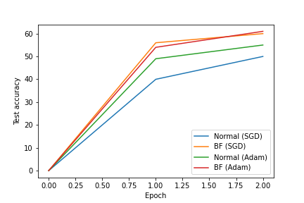
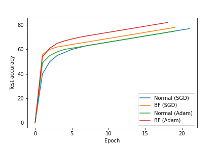
Figure 2 reports the test accuracy of the original model and the butterfly model. The black vertical lines in Figures 2 denote the error bars corresponding to standard deviation, and the values above the rectangles denote the average accuracy. In Figure 3 observe that the test accuracy for the butterfly model trained with stochastic gradient descent is even better than the original model trained with Adam in the first few epochs. Figure 14 in Appendix D.1 compares the test accuracy in the the first 20 epochs of the original and butterfly model. The results for the NLP tasks in the interest of space are reported in Figure 11, Appendix D.1. The training and inference times required for the original model and the butterfly model in each of these experiments are reported in Figures 12 and 13 in Appendix D.1. We remark that the modified architecture is also trained for fewer epochs. In almost all the cases the modified architecture does better than the normal architecture, both in the rate of convergence and in the final accuracy/ score. Moreover, the training time for the modified architecture is less.
5.2 Encoder-Decoder Butterfly network with Synthetic Gaussian and Real Data
This experiment tests whether gradient descent based techniques can be used to train an auto-encoder with a truncated butterfly gadget (see Section 4). Five types of data matrices are tested: two are random and three are constructed using standard public real image datasets. For the matrices constructed from the image datasets, the input coordinates are randomly permuted, which ensures the network cannot take advantage of the spatial structure in the data.
Table 2 summarizes the data attributes. Gaussian and Gaussian are Gaussian matrices with rank and respectively. A Rank Gaussian matrix is constructed as follows: orthogonal vectors of size are sampled at random and the columns of the matrix are determined by taking random linear combinations of these vectors, where the coefficients are chosen independently and uniformly at random from the Gaussian distribution with mean and variance . The data matrix for MNIST is constructed as follows: each row corresponds to an image represented as a matrix (pixels) sampled uniformly at random from the MNIST database of handwritten digits LeCun and Cortes 2010 which is extended to a matrix by padding numbers close to zero and then represented as a vector of size in column-first ordering88 8 Close to zero entries are sampled uniformly at random according to a Gaussian distribution with mean zero and variance .. Similar to the MNIST every row of the data matrix for Olivetti corresponds to an image represented as a matrix sampled uniformly at random from the Olivetti faces data set Cambridge 1994, which is represented as a vector of size in column-first ordering. Finally, for HS-SOD the data matrix is a matrix sampled uniformly at random from HS-SOD – a dataset for hyperspectral images from natural scenes Imamoglu et al. 2018.
| Name | rank | ||
|---|---|---|---|
| Gaussian 1 | 1024 | 1024 | 32 |
| Gaussian 2 | 1024 | 1024 | 64 |
| MNIST | 1024 | 1024 | 1024 |
| Olivetti | 1024 | 4096 | 1024 |
| HS-SOD | 1024 | 768 | 768 |
For each of the data matrices the loss obtained via training the truncated butterfly network with the Adam optimizer is compared to (denoted as PCA) and where is an matrix sampled from the FJLT distribution (denoted as FJLT+PCA).99 9 PCA stands for principal component analysis which is a standard way to compute . Figures 4 and 5 reports the loss on Gaussian 1 and MNIST respectively, whereas Figure 15 in Appendix D.2 reports the loss for the remaining data matrices. Observe that for all values of the loss for the encoder-decoder butterfly network is almost equal to , and is in fact for small and large values of .


5.3 Two-phase Learning
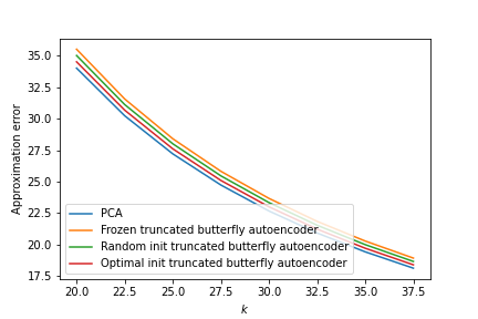
This experiment is similar to the experiment in Section 5.2 but the training in this case is done in two phases. In the first phase, is fixed and the network is trained to determine an optimal and . In the second phase, the optimal and determined in phase one are used as the initialization, and the network is trained over and to minimize the loss. Theorem 1 ensures worst-case guarantees for this two phase training (see below the theorem). Figure 6 reports the approximation error of an image from Imagenet. The red and green lines in Figure 6 correspond to the approximation error at the end of phase one and two respectively.
6 Sketching for Low-Rank Matrix Decomposition
This experiment was inspired by the recent influential work by Indyk et al. 2019, which considers a supervised learning approach to compute an pre-conditioning matrix , where , such that for , the best rank approximation of from the rows of (denoted ) is optimized. The matrix has a fixed sparse structure determined a priory as in (Clarkson and Woodruff 2009), and the non-zero entries are learned to minimize the loss over a training set of matrices. The results in (Indyk et al. 2019) suggest that a learned matrix significantly improves the guarantee compared to a random sketching matrix as in (Clarkson and Woodruff 2009). Our setting is similar to that in (Indyk et al. 2019), except that is now represented as an truncated butterfly gadget. Our experiments on several datasets show that indeed a learned truncated butterfly gadget does better than a random matrix, and even a learned as in (Indyk et al. 2019).
Setup: Suppose are training matrices sampled from a distribution . Then a is computed that minimizes the following empirical loss
| (2) |
We compute using truncated SVD of (as in Algorithm 1, (Indyk et al. 2019)). The matrix is learned by the back-propagation algorithm that uses a differentiable SVD implementation to calculate the gradients, followed by optimization with Adam such that the butterfly structure of is maintained. The learned can be used as the pre-processing matrix for any matrix in the future. The test error for a matrix and a test set is defined as follows:
where .
Experiments and Results: The experiments are performed on the datasets shown in Table 3. In HS-SOD (Imamoglu et al. 2018) and CIFAR-10 (Krizhevsky 2012) 400 training matrices (), and 100 test matrices are sampled, while in Tech 200 (Davido et al. 2004), training matrices (), and 95 test matrices are sampled. In Tech, each matrix has 835,422 rows but on average only 25,389 rows and 195 columns contain non-zero entries. For the same reason as in Section 5.2 in each dataset, the coordinates of each row are randomly permuted. Some of the matrices in the datasets have much larger singular values than the others, and to avoid imbalance in the dataset, the matrices are normalized so that their top singular values are all equal, as done in (Indyk et al. 2019).
| Name | ||
|---|---|---|
| HS-SOD 1 | 1024 | 768 |
| CIFAR-10 | 32 | 32 |
| Tech | 25,389 | 195 |
For each of the datasets, the test error for the learned via our truncated butterfly structure is compared to the test errors for the following three cases: 1) is a learned as a sparse sketching matrix as in Indyk et al. 2019, b) is a random sketching matrix as in Clarkson and Woodruff 2009, and c) is an Gaussian matrix. Figure 8 compares the test error for , and , where . Figure 16 in Appendix E compares the test errors of the different methods in the extreme case when , and Figure 17 in Appendix E compares the test errors of the different methods for various values of . Table 4 in Appendix E reports the test error for different values of and . Figure 18 in Appendix E shows the test error for and during the training phase on HS-SOD. In Figure 18 it is observed that the butterfly learned is able to surpass sparse learned after merely a few iterations.


Figure 8 compares the test error for the learned via our truncated butterfly structure to a learned matrix with non-zero entries in each column – the non-zero location for each column are chosen uniformly at random. The reported test errors are on HS-SOD, when and . Interestingly, the error for butterfly learned is not only less than the error for sparse learned ( as in (Indyk et al. 2019)) but also less than than the error for dense learned (). In particular, our results indicate that using a learned butterfly sketch can significantly reduce the approximation loss compared to using a learned sparse sketching matrix.
7 Conclusion
Discussion: Among other things, this work showed that it is beneficial to replace dense linear layer in deep learning architectures with a more compact architecture (in terms of number of parameters), using truncated butterfly networks. This approach is justified using ideas from efficient matrix approximation theory from the last two decades. however, results in additional logarithmic depth to the network. This issue raises the question of whether the extra depth may harm convergence of gradient descent optimization. To start answering this question, we show, both empirically and theoretically, that in linear encoder-decoder networks in which the encoding is done using a butterfly network, this typically does not happen. To further demonstrate the utility of truncated butterfly networks, we consider a supervised learning approach as in Indyk et al. 2019, where we learn how to derive low rank approximations of a distribution of matrices by multiplying a pre-processing linear operator represented as a butterfly network, with weights trained using a sample of the distribution.
Future Work: The main open questions arising from the work are related to better understanding the optimization landscape of butterfly networks. The current tools for analysis of deep linear networks do not apply for these structures, and more theory is necessary. It would be interesting to determine whether replacing dense linear layers in any network, with butterfly networks as in Section 3.2 harms the convergence of the original matrix. Another direction would be to check empirically whether adding non-linear gates between the layers (logarithmically many) of a butterfly network improves the performance of the network. In the experiments in Section 5.1, we have replaced a single dense layer by our proposed architecture. It would be worthwhile to check whether replacing multiple dense linear layers in the different architectures harms the final accuracy. Similarly, it might be insightful to replace a convolutional layer by an architecture based on truncated butterfly network. Finally, since our proposed replacement reduces the number of parameters in the network, it might be possible to empirically show that the new network is more resilient to over-fitting.
Acknowledgements
This project has received funding from European Union’s Horizon 2020 research and innovation program under grant agreement No 682203 -ERC-[ Inf-Speed-Tradeoff].
References
- Ailon and Chazelle [2009] Nir Ailon and Bernard Chazelle. The fast johnson–lindenstrauss transform and approximate nearest neighbors. SIAM Journal on Computing, 39(1):302–322, 2009.
- Ailon and Liberty [2009] Nir Ailon and Edo Liberty. Fast dimension reduction using rademacher series on dual BCH codes. Discrete and Computational Geometry, 42(4):615–630, 2009.
- Ailon et al. [2021] Nir Ailon, Omer Leibovitch, and Vineet Nair. Code for Sparse Linear Networks with a Fixed Butterfly Structure: Theory and Practice. https://github.com/leibovit/Sparse-Linear-Networks, 2021.
- Akbik et al. [2018] Alan Akbik, Duncan Blythe, and Roland Vollgraf. Contextual string embeddings for sequence labeling. In International Conference on Computational Linguistics COLING, pages 1638–1649, 2018.
- Akbik et al. [2019] Alan Akbik, Tanja Bergmann, and Roland Vollgraf. Pooled contextualized embeddings for named entity recognition. In Conference of the North American Chapter of the Association for Computational Linguistics NAACL, page 724–728, 2019.
- Alizadeh et al. [2020] Keivan Alizadeh, Prabhu Anish, Farhadi Ali, and Rastegari Mohammad. Butterfly transform: An efficient fft based neural architecture design. In Conference on Computer Vision and Pattern Recognition (CVPR), 2020.
- Baldi and Hornik [1989] Pierre Baldi and Kurt Hornik. Neural networks and principal component analysis: Learning from examples without local minima. Neural Networks, 2(1):53–58, 1989.
- Cambridge [1994] AT&T Laboratories Cambridge. The olivetti faces dataset, 1994.
- Cheng et al. [2015] Yu Cheng, Felix X. Yu, Rogério Schmidt Feris, Sanjiv Kumar, Alok N. Choudhary, and Shih-Fu Chang. An exploration of parameter redundancy in deep networks with circulant projections. In International Conference on Computer Vision, ICCV, pages 2857–2865. IEEE Computer Society, 2015.
- Clarkson and Woodruff [2009] Kenneth L. Clarkson and David P. Woodruff. Numerical linear algebra in the streaming model. In Michael Mitzenmacher, editor, Proceedings of the 41st Annual ACM Symposium on Theory of Computing, STOC 2009, pages 205–214. ACM, 2009.
- Cooley and Tukey [1965] J.W. Cooley and J.W. Tukey. An algorithm for the machine calculation of complex fourier series. Mathematics of Computation, 19(90):297–301, 1965.
- Dao et al. [2019] Tri Dao, Albert Gu, Matthew Eichhorn, Atri Rudra, and Christopher Ré. Learning fast algorithms for linear transforms using butterfly factorizations. In Kamalika Chaudhuri and Ruslan Salakhutdinov, editors, International Conference on Machine Learning, ICML, volume 97 of Proceedings of Machine Learning Research, pages 1517–1527. PMLR, 2019.
- Dao et al. [2020] Tri Dao, Nimit Sharad Sohoni, Albert Gu, Matthew Eichhorn, Amit Blonder, Megan Leszczynski, Atri Rudra, and Christopher R ’e. Kaleidoscope: An efficient, learnable representation for all structured linear maps. In International Conference on Learning Representations, ICLR, 2020.
- Davido et al. [2004] D. Davido, E. Gabrilovich, and S. Markovitch. Parameterized generation of labeled datasets for text categorization based on a hierarchical directory. In International ACM SIGIR Conference on Research and Development in Information Retrieval, SIGIR, pages 250–257, 2004.
- Deng et al. [2009] J. Deng, W. Dong, R. Socher, L.-J. Li, K. Li, and L. Fei-Fei. ImageNet: A Large-Scale Hierarchical Image Database. In Conference on Computer Vision and Pattern Recognition, CVPR. IEEE Computer Society, 2009.
- Denil et al. [2013] Misha Denil, Babak Shakibi, Laurent Dinh, Marc’Aurelio Ranzato, and Nando de Freitas. Predicting parameters in deep learning. In Advances in Neural Information Processing Systems NeurIPS, pages 2148–2156, 2013.
- Ding et al. [2017] Caiwen Ding, Siyu Liao, Yanzhi Wang, Zhe Li, Ning Liu, Youwei Zhuo, Chao Wang, Xuehai Qian, Yu Bai, Geng Yuan, Xiaolong Ma, Yipeng Zhang, Jian Tang, Qinru Qiu, Xue Lin, and Bo Yuan. Circnn: accelerating and compressing deep neural networks using block-circulant weight matrices. In IEEE/ACM International Symposium on Microarchitecture, MICRO, pages 395–408. ACM, 2017.
- He et al. [2016] Kaiming He, Xiangyu Zhang, Shaoqing Ren, and Jian Sun. Identity mappings in deep residual networks. In European Conference on Computer Vision, ECCV, volume 9908 of Lecture Notes in Computer Science, pages 630–645. Springer, 2016.
- Hu et al. [2020] Jie Hu, Li Shen, Samuel Albanie, Gang Sun, and Enhua Wu. Squeeze-and-excitation networks. IEEE Transactions on Pattern Analysis and Machine Intelligence, 42(8):2011–2023, 2020.
- Imamoglu et al. [2018] N. Imamoglu, Y. Oishi, X. Zhang, Y. Fang G. Ding, T. Kouyama, and R. Nakamura. Hyperspectral image dataset for benchmarking on salient object detection. In International Conference on Quality of Multimedia Experience, QoME, pages 1–3, 2018.
- Indyk et al. [2019] Piotr Indyk, Ali Vakilian, and Yang Yuan. Learning-based low-rank approximations. In Hanna M. Wallach, Hugo Larochelle, Alina Beygelzimer, Florence d’Alché-Buc, Emily B. Fox, and Roman Garnett, editors, Advances in Neural Information Processing Systems NeurIPS, pages 7400–7410, 2019.
- Jain et al. [2020] Vishesh Jain, Natesh Pillai, and Aaron Smith. Kac meets johnson and lindenstrauss: a memory-optimal, fast johnson-lindenstrauss transform. arXiv, 03 2020.
- Johnson and Lindenstrauss [1984] William Johnson and Joram Lindenstrauss. Extensions of lipschitz maps into a hilbert space. Contemporary Mathematics, 26:189–206, 01 1984. doi: 10.1090/conm/026/737400.
- Kawaguchi [2016] Kenji Kawaguchi. Deep learning without poor local minima. In Advances in Neural Information Processing Systems NeurIPS, pages 586–594, 2016.
- Krahmer and Ward [2011] Felix Krahmer and Rachel Ward. New and improved johnson–lindenstrauss embeddings via the restricted isometry property. SIAM Journal on Mathematical Analysis, 43:1269–1281, 06 2011. doi: 10.1137/100810447.
- Krizhevsky [2012] Alex Krizhevsky. Learning multiple layers of features from tiny images. University of Toronto, 2012.
- LeCun and Cortes [2010] Yann LeCun and Corinna Cortes. MNIST handwritten digit database, 2010.
- Lee et al. [2019] Namhoon Lee, Thalaiyasingam Ajanthan, and Philip H. S. Torr. Snip: single-shot network pruning based on connection sensitivity. In International Conference on Learning Representations, ICLR. OpenReview.net, 2019.
- Li and Yang [2017] Yingzhou Li and Haizhao Yang. Interpolative butterfly factorization. SIAM Journal on Scientific Computing, 39(2), 2017.
- Li et al. [2015] Yingzhou Li, Haizhao Yang, Eileen R. Martin, Kenneth L. Ho, and Lexing Ying. Butterfly factorization. Multiscale Model. Simul., 13(2):714–732, 2015.
- Li et al. [2018] Yingzhou Li, Xiuyuan Cheng, and Jianfeng Lu. Butterfly-net: Optimal function representation based on convolutional neural networks. CoRR, abs/1805.07451, 2018.
- Lu et al. [2016] Zhiyun Lu, Vikas Sindhwani, and Tara N. Sainath. Learning compact recurrent neural networks. In International Conference on Acoustics, Speech and Signal Processing, ICASSP, pages 5960–5964. IEEE, 2016.
- Marcus et al. [1993] Mitchell P. Marcus, Beatrice Santorini, and Mary Ann Marcinkiewicz. Building a large annotated corpus of English: The Penn Treebank. Computational Linguistics, 19(2):313–330, 1993. URL https://www.aclweb.org/anthology/J93-2004.
- Michielssen and Boag [1996] E. Michielssen and A. Boag. A multilevel matrix decomposition algorithm for analyzing scattering from large structures. IEEE Transactions on Antennas and Propagation, 44(8):1086–1093, 1996.
- Mocanu et al. [2018] Decebal Constantin Mocanu, Elena Mocanu, Peter Stone, Phuong H. Nguyen, Madeleine Gibescu, and Antonio Liotta. Scalable training of artificial neural networks with adaptive sparse connectivity inspired by network science. Nature Communications, 9:2383, 2018. doi: 10.1038/s41467-018-04316-3.
- Moczulski et al. [2016] Marcin Moczulski, Misha Denil, Jeremy Appleyard, and Nando de Freitas. ACDC: A structured efficient linear layer. In Yoshua Bengio and Yann LeCun, editors, International Conference on Learning Representations, ICLR, 2016.
- O’Neil et al. [2010] Michael O’Neil, Franco Woolfe, and Vladimir Rokhlin. An algorithm for the rapid evaluation of special function transforms. Applied and Computational Harmonic Analysis, 28(2):203 – 226, 2010.
- Sainath et al. [2013] Tara N. Sainath, Brian Kingsbury, Vikas Sindhwani, Ebru Arisoy, and Bhuvana Ramabhadran. Low-rank matrix factorization for deep neural network training with high-dimensional output targets. In International Conference on Acoustics, Speech and Signal Processing, ICASSP, pages 6655–6659. IEEE, 2013.
- Sarlós [2006] Tamás Sarlós. Improved approximation algorithms for large matrices via random projections. In IEEE Symposium on Foundations of Computer Science FOCS, pages 143–152. IEEE Computer Society, 2006.
- Seljebotn [2012] D. S. Seljebotn. WAVEMOTH-FAST SPHERICAL HARMONIC TRANSFORMS BY BUTTERFLY MATRIX COMPRESSION. The Astrophysical Journal Supplement Series, 199(1):5, 2012.
- Sindhwani et al. [2015] Vikas Sindhwani, Tara N. Sainath, and Sanjiv Kumar. Structured transforms for small-footprint deep learning. In Corinna Cortes, Neil D. Lawrence, Daniel D. Lee, Masashi Sugiyama, and Roman Garnett, editors, Advances in Neural Information Processing Systems NeurIPS, pages 3088–3096, 2015.
- Tan and Le [2019] Mingxing Tan and Quoc V. Le. Efficientnet: Rethinking model scaling for convolutional neural networks. In Kamalika Chaudhuri and Ruslan Salakhutdinov, editors, International Conference on Machine Learning, ICML, volume 97 of Proceedings of Machine Learning Research, pages 6105–6114. PMLR, 2019.
- Thomas et al. [2018] Anna T. Thomas, Albert Gu, Tri Dao, Atri Rudra, and Christopher Ré. Learning compressed transforms with low displacement rank. In Advances in Neural Information Processing Systems NeurIPS, pages 9066–9078, 2018.
- Tjong Kim Sang and De Meulder [2003] Erik F. Tjong Kim Sang and Fien De Meulder. Introduction to the CoNLL-2003 shared task: Language-independent named entity recognition. In Conference on Natural Language Learning at HLT-NAACL, pages 142–147, 2003. URL https://www.aclweb.org/anthology/W03-0419.
- Verdenius et al. [2020] Stijn Verdenius, Maarten Stol, and Patrick Forré. Pruning via iterative ranking of sensitivity statistics. CoRR, abs/2006.00896, 2020.
- Wang et al. [2020] Chaoqi Wang, Guodong Zhang, and Roger B. Grosse. Picking winning tickets before training by preserving gradient flow. In International Conference on Learning Representations, ICLR. OpenReview.net, 2020.
- Yang et al. [2015] Zichao Yang, Marcin Moczulski, Misha Denil, Nando de Freitas, Alexander J. Smola, Le Song, and Ziyu Wang. Deep fried convnets. In IEEE International Conference on Computer Vision, ICCV, pages 1476–1483. IEEE Computer Society, 2015.
- Ye et al. [2018] Jinmian Ye, Linnan Wang, Guangxi Li, Di Chen, Shandian Zhe, Xinqi Chu, and Zenglin Xu. Learning compact recurrent neural networks with block-term tensor decomposition. In Conference on Computer Vision and Pattern Recognition, CVPR, pages 9378–9387. IEEE Computer Society, 2018.
Appendix A Butterfly Diagram from Section 1
Figure 9 referred to in the introduction is given here.


Appendix B Proof of Proposition 3.1
The proof of the proposition will use the following well known fact (Lemma B.1 below) about FJLT (more generally, JL) distributions (see Ailon and Chazelle 2009, Ailon and Liberty 2009, Krahmer and Ward 2011).
Lemma B.1.
Let be a unit vector, and let be a matrix drawn from an FJLT distribution. Then for all with probability at least :
| (3) |
By Lemma B.1 we have that with probability at least ,
| (4) |
Henceforth, we condition on the event . Therefore, by the definition of spectral norm of :
| (5) |
Now apply Lemma B.1 again on the vector and transformation to get that with probability at least ,
| (6) |
Henceforth, we condition on the event . To bound the last right hand side, we use the triangle inequality together with (5):
| (7) |
| (8) |
Finally,
| (9) | |||||
where the first inequality is from the triangle inequality together with (5) and (8), and the second inequality is from the bound on . The proposition is obtained by adjusting the constants hiding inside the notation in the exponent in the proposition statement.
Appendix C Proof of Theorem 1
We first note that our result continues to hold even if in the theorem is replaced by any structured matrix. For example the result continues to hold if is an matrix with one non-zero entry per column, as is the case with a random sparse sketching matrix Clarkson and Woodruff 2009. We also compare our result with that Baldi and Hornik 1989, Kawaguchi 2016.
Comparison with Baldi and Hornik 1989 and Kawaguchi 2016: The critical points of the encoder-decoder network are analyzed in Baldi and Hornik 1989. Suppose the eigenvalues of are and . Then they show that corresponding to a critical point there is an such that the loss at this critical point is equal to , and the critical point is a local/global minima if and only if . Kawaguchi 2016 later generalized this to prove that a local minima is a global minima for an arbitrary number of hidden layers in a linear neural network if . Note that since and in Theorem 1, replacing by in Baldi and Hornik 1989 or Kawaguchi 2016 does not imply Theorem 1 as it is.
Next, we introduce a few notation before delving into the proof. Let , and is the entries of arranged as a vector in column-first ordering, and denote the partial derivative of with respect to the parameters in and respectively. Notice that and are row vectors of size and respectively. Also, let denote the projection matrix of , and hence if is a matrix with full column-rank then . The identity matrix is denoted as , and for convenience of notation let . First we prove the following lemma which gives an expression for and if and are zero.
Lemma C.1 (Derivatives with respect to and ).
- 1.
, and
- 2.
Proof.
- 1.
Since ,
- 2.
Similarly,
∎
Assume the rank of is equal to . Hence there is an invertible matrix such that is such that the last columns of are zero and the first columns of are linearly independent (via Gauss elimination). Let . Without loss of generality it can be assumed , and , by restricting restricting to its first columns (as the remaining are zero) and to its first rows. Hence, is a full column-rank matrix of rank , and . Claims C.1 and C.2 aid us in the completing the proof of the theorem. First the proof of theorem is completed using these claims, and at the end the two claims are proved.
Claim C.1 (Representation at the critical point).
- 1.
- 2.
Claim C.2.
- 1.
- 2.
We denote as for convenience. Since is a real symmetric matrix, there is an orthogonal matrix consisting of the eigenvectors of , such that , where is a diagonal matrix whose first diagonal entries are and the remaining entries are zero. Let be the columns of . Then for , is the eigenvector of corresponding to the eigenvalue , and are the eigenvectors of corresponding to the eigenvalue .
Note that , and from part two of Claim C.2 we have
| (10) | ||||
| (11) | ||||
| (12) |
Since commutes with , is a block-diagonal matrix comprising of two blocks and : the first block is an diagonal block, and is a matrix. Since is orthogonal projection matrix of rank its eigenvalues are with multiplicity and with multiplicity . Hence at most diagonal entries of are and the remaining are . Finally observe that
The second line in the above equation follows using the fact that , the third line in the above equation follows by substituting (from part two of Claim C.1), and the last line follows from part two of Claim C.2. Substituting , and in the above equation we have,
The last line the above equation follows from the fact that . From the structure of and it follows that there is a subset , such that . Hence, .
Since , there is a invertible matrix such that
where is a block-diagonal matrix consisting of two blocks and : is equal to , and is an orthogonal matrix, and is such that and . The relation for in the above equation follows from part one of Claim C.1. Note that if , then , that is consists of indices corresponding to eigenvectors of non-zero eigenvalues.
Recall that was obtained by truncating the last zero rows of , where was a invertible matrix simulating the Gaussian elimination. Let denoted the matrix obtained by augmenting the columns of with zero columns. Then
Similarly, there is a matrix such that
where denotes the matrix obtained by augmenting the rows of with the rows of . Now suppose , and hence . Then we will show that there are matrices and arbitrarily close to and respectively such that if then . There is an , and such that ( could also be zero). Denote the columns of the matrix as , and observe that for (from the structure of ). For let . Define as the matrix which is equal to except that the column vector in is replaced by in . Since and , and . Define
and let . Now observe that, , and that
Since can be set arbitrarily close to zero, it can be concluded that there are points in the neighbourhood of such that the loss at these points are less than . Further, since is convex with respect to the parameters in (respectively ), when the matrix is fixed (respectively is fixed) is not a local maximum. Hence, if then represents a saddle point, and in particular is local/global minima if and only if .
Proof of Claim C.1.
Proof of Claim C.2.
Since is zero, from the first part of Lemma C.1 the following holds,
| (17) |
Substituting as in Equation 13, and multiplying Equation 17 by on both the sides from the left Equation 18 follows.
| (18) |
Taking transpose of the above equation we have,
| (19) |
From part 1 of Claim C.1, it follows that has full row-rank, and hence is invertible. Multiplying the inverse of from the right on both sides and multiplying from the left on both sides of the above equation we have,
| (20) |
This proves part one of the claim. Moreover, multiplying Equation 19 by from the right on both sides
The second line the above equation follows by substituting (from part 2 of Claim C.1). Substituting in the above equation we have
Since , and , we also have . ∎
Appendix D Additional Tables and Plots related to Dense Layer Replacement
D.1 Plots from Section 5.1
Figure 10 displays the number of parameter in the original model and the butterfly model. Figure 11 reports the results for the NLP tasks done as part of experiment in Section 5.1. Figures 12 and 13 reports the training and inference times required for the original model and the butterfly model in each of the experiments. The training and and inference times in Figures 12 and 13 are averaged over 100 runs. Figure 14 is the same as the right part of Figure 3 but here we compare the test accuracy of the original and butterfly model for the the first 20 epochs.


D.2 Plots from Section 5.2
Figure 15 reports the losses for the Gaussian 2, Olivetti, and Hyper data matrices.


Appendix E Additional Plots related to Sketching
In this section we state a few additional cases that were done as part of the experiment in Section 6. Figure 16 compares the test errors of the different methods in the extreme case when . Figure 17 compares the test errors of the different methods for various values of . Figure 18 shows the test error for and during the training phase on HS-SOD. Observe that the butterfly learned is able to surpass sparse learned after a merely few iterations. Finally Table 4 compares the test error for different values of and .


| k, , Sketch | Hyper | Cifar-10 | Tech | ||||||||||||
|---|---|---|---|---|---|---|---|---|---|---|---|---|---|---|---|
|
|
|
| ||||||||||||
|
|
|
| ||||||||||||
|
|
|
| ||||||||||||
|
|
|
| ||||||||||||
|
|
| |||||||||||||
|
|
| |||||||||||||
|
|
| |||||||||||||
|
|
| |||||||||||||
|
|
|
Appendix F Bound on Number of Effective Weights in Truncated Butterfly Network
A butterfly network for dimension , which we assume for simplicity to be an integral power of , is layers deep. Let denote the integer . The set of nodes in the first (input) layer will be denoted here by . They are connected to the set of nodes from the next layer, and so on until the nodes of the output layer. Between two consecutive layers and , there are weights, and each node in is adjacent to exactly two nodes from .
When truncating the network, we discard all but some set of at most nodes in the last layer. These nodes are connected to a subset of at most nodes from the preceding layer using at most weights. By induction, for all , the set of nodes is of size at most , and is connected to the set using at most weights.
Now take . By the above, the total number of weights that can participate in a path connecting some node in with some node in is at most .
From the other direction, the total number of weights that can participate in a path connecting any node from with any node from is times the number of layers in between, or more precisely:
The total is , as required.