An analytic study on the excited states of holographic superconductors

It has been shown numerically that, for both the ground and excited states of the holographic superconductor, there exists a critical chemical potential $\mu_{c}$ (a critical temperature $T_{c}$), above (below) which the scalar field begins to condensate due to the spontaneously broken $U(1)$ gauge symmetry WangJHEP2020. Since the scalar field $\psi=0$ at the critical chemical potential $\mu_{c}$, as $\mu\rightarrow\mu_{c}$ below the critical point, Eq. (7) reduces to $\phi^{\prime\prime}=0$, which has a solution

Here we have introduced a dimensionless quantity $\lambda\equiv\mu/r_{+c}=\rho/r^{2}_{+c}$, where $r_{+c}$ is the radius of the horizon at the critical point.

According to the asymptotical behavior given by Eq. (5), we take the scalar field as

with the boundary condition $F(0)=1$. By inserting Eqs. (8) and (9) into Eq. (6), we obtain the equation of motion for the trial function $F(z)$

near the critical point, and where we have defined

By making use of the Sturm-Liouville approach Gelfand-Fomin, the eigenvalue $\mu/r_{+}$ may be achieved from the extremal values of the following function by virtue of the Rayleigh Quotient

where we have employed the boundary condition

To be specific, we take $m^{2}L^{2}=-2$ for the calculations we conducted in this section. It is obvious that for this case, the condition $T(0)F(0)F^{\prime}(0)=0$ is not satisfied automatically for the operator $O_{1}$ since the leading order contribution from $T(z)$ is $2(\Delta_{-}-1)=0$, as $z\rightarrow 0$; while the aforementioned condition is satisfied automatically for the operator $O_{2}$ since $2(\Delta_{+}-1)=2>1$. Thus, as discussed in Refs. HFLi; WangSPJ; LvPLB2020, we have to impose an additional Neumann boundary condition $F^{\prime}(0)=0$ for the operator $O_{1}$ but need not impose any restrictions on $F^{\prime}(z)$ for the operator $O_{2}$.

In order to analytically investigate the excited states of the holographic superconductors by using the Sturm-Liouville method, we shall include more higher orders of $z$ in the trial function $F(z)$. As a concrete example, we calculate the case for the operator $O_{1}$. From the above discussion, we should impose the Neumann boundary condition $F^{\prime}(0)=0$ and choose the third order trial function

which leads to

Computing the extremal values of the above expression, we can obtain the dimensionless critical chemical potential from the ground state to the second excited state, i.e., $\mu_{c}^{(0)}/r_{+}=1.121$ at $a_{2}=0.496$ and $a_{3}=-0.271$, $\mu_{c}^{(1)}/r_{+}=6.714$ at $a_{2}=15.632$ and $a_{3}=-12.681$, and $\mu_{c}^{(2)}/r_{+}=18.478$ at $a_{2}=39.772$ and $a_{3}=-57.299$. Comparing with the numerical results in WangJHEP2020, we only obtain the first three lowest-lying modes by using the third order trial function $F(z)$.

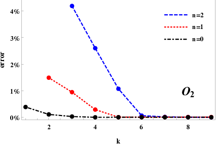
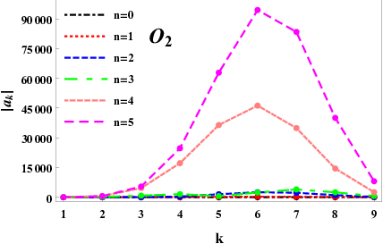
In order to give the higher excited state by using the analytic Sturm-Liouville method, we include the ninth order of $z$ in the trial function $F(z)$, i.e., $F(z)=1-\sum_{k=2}^{k=9}a_{k}z^{k}$ for the operator $O_{1}$, and $F(z)=1-\sum_{k=1}^{k=9}a_{k}z^{k}$ for the operator $O_{2}$. As a matter of fact, just as shown in Fig. 1 for the first three lowest-lying modes, the percentage errors in the analytic estimation for the critical chemical potential of the scalar operators $O_{1}$ and $O_{2}$ drop quickly with the order of the expansion, which indicates that the trial function $F(z)$ with the ninth order of $z$ will lead to a more precise estimation. The dimensionless critical chemical potential $\mu_{c}/r_{+}$ and corresponding value of $a_{k}$ from the ground state to the fifth excited state are tabulated in Tables 1 and 2. Moreover, to check the convergence of the high order expansion directly, in Fig. 2 we also exhibit the value of $|a_{k}|$ as a function of $k$ for the scalar operators $O_{1}$ and $O_{2}$, which implies that the expansion of the trial function is convergent. Comparing with the analytical result obtained from the third order trial function $F(z)$ in Eq. (14), we find that the value of $\mu_{c}/r_{+}$ with the ninth order trial function is much closer to the numerical result given in Tables 1 and 2, even in the fifth excited state. The tiny error indicates that the Sturm-Liouville method with the higher order of $z$ in the trial function $F(z)$ can not only find the most stable mode, but also can find the metastable modes just like the spectral method did in WangJHEP2020.

From Tables 1 and 2, we observe that the critical chemical potential $\mu_{c}$ increases with increasing the number of nodes $n$ for both the operators $O_{1}$ and $O_{2}$, which agrees well with the fact that the ground state first appears with the decrease of the temperature and the solutions of the first-excited state begin to develop by further decreasing the temperature to the critical temperature of the first-excited state. This can be used to back up the numerical finding given in Ref. WangJHEP2020 that there exists a lower critical temperature in the corresponding excited state. Using the analytic results obtained by the Sturm-Liouville method, we can express the relation between $\mu_{c}/r_{+}$ and $n$ as

which is in very good agreement with the numeric results given in WangJHEP2020, and shows that for both operators the difference of the dimensionless critical chemical potential $\mu_{c}/r_{+}$ between the consecutive states is around 5.

In the vicinity of the critical point, the condensate for the scalar operator $O_{i}$ is small. Therefore, we can expand $\phi(z)$ in small $\langle O_{i}\rangle$ as

with the boundary condition $\chi(1)=\chi^{\prime}(1)=0$ at the event horizon Siopsis. Substituting the above expression and function (9) into Eq. (7), we obtain the equation of motion for $\chi(z)$

Making integration for both sides of the above equation, we obtain

According to the asymptotic behavior given in Eq. (5), we can expand $\phi(z)$ near $z\rightarrow 0$ as

From the coefficients of the $z^{1}$ term, we have

where the critical temperature is given by

with the extremal values $\lambda_{ext}$ of the expression (12). From Eq. (23), it is shown clearly that the phase transition of the holographic s-wave superconductors belongs to the second order and the critical exponent of the system takes the mean field value $1/2$, even in the excited states.

To be specific, we take the scalar field mass as $m^{2}L^{2}=-2$ in the holographic s-wave superconductors. We have calculated the first three lowest-lying modes, for the operator $O_{1}$

and for the operator $O_{2}$

and both of which agree well with the numerical data obtained by the spectral method in WangJHEP2020, especially the critical temperatures $T_{c}$. For the ground state, comparing with the analytical results from the second order trial function $F(z)$ Siopsis; ZengGao; GangopadhyayR; PanJWC, i.e., $T_{c}^{(0)}\approx 0.225\rho^{1/2}$ for the operator $O_{1}$ and $T_{c}^{(0)}\approx 0.117\rho^{1/2}$ for the operator $O_{2}$, we observe that the values of $T_{c}$ with the ninth order trial function are much more closer to the numerical findings. On the other hand, using the analytic expression (II.1) and numerical results, we plot the values of the dimensionless critical temperature $T_{c}/\rho^{1/2}$ in function of $n$ for the scalar operators $O_{1}$ and $O_{2}$ in Fig. 3, which shows that the critical temperature decreases with the increase of $n$. This means that the excited state has a lower critical temperature than the corresponding ground state.

Through the above analytic calculations we have confirmed, on one hand, that the condensate of the excited states is smaller (larger) than that of the ground state for the operator $O_{1}$ ($O_{2}$); on the other hand, that the Sturm-Liouville method is a very powerful approach to analytically investigate the holographic s-wave superconductors for both the ground and excited states.

Similarly to the analysis provided in the previous section, if $\mu\leq\mu_{c}$, the vector field $\rho_{x}=0$. Therefore, below the critical point, Eq. (43) becomes $A_{t}^{\prime\prime}=0$, which leads to the same solution as in (8) for $\phi$, i.e.,

with a dimensionless quantity $\lambda\equiv\mu/r_{+c}=\rho/r^{2}_{+c}$.

Taking into account the asymptotic behavior from Eq. (41), we assume that the vector field $\rho_{x}$ takes the form

where the trial function $F(z)$ with the boundary conditions $F(0)=1$ satisfies the following equation of motion

with

Here, the function $V(z)$ is defined in Eq. (11). Following the Sturm-Liouville method Gelfand-Fomin, the eigenvalues of $\mu/r_{+}$ can be obtained from variation of the following function

It should be noted that $[P(z)F(z)F^{\prime}(z)]|_{0}^{1}=0$, because of the fact that $P(1)\equiv 0$ and $P(0)\equiv 0$ for the case of $\Delta=(1+\sqrt{1+4m^{2}L^{2}})/2$. Thus, similarly to the operator $O_{2}$ in the holographic s-wave superconductors, we require $F(z)$ to obey the Dirichlet boundary condition $F(0)=1$ rather than the Neumann boundary condition $F^{\prime}(0)=0$.

To be specific, in the following calculations we take the mass of the vector field as $m^{2}L^{2}=3/4$, and the other choices of the mass will not change our results qualitatively. In order to obtain the higher excited states of the holographic p-wave superconductors, we include the ninth order of $z$ in the trial function $F(z)$, i.e., $F(z)=1-\sum_{k=1}^{k=9}a_{k}z^{k}$ for the operator $O_{x}$, which will lead to a more precise estimation for the critical chemical potential, just as shown in Fig. 4 for the first three lowest-lying modes, where the percentage errors in the analytic estimation drop quickly with the order of the expansion. We give the dimensionless critical chemical potential $\mu_{c}/r_{+}$ and corresponding value of $a_{k}$ from the ground state to the fifth excited state in Table 3, and plot the value of $|a_{k}|$ in function of $k$ in Fig. 5 which indicates the convergence of the high order expansion for the trial function $F(z)$. It is shown clearly that, the agreement between the analytic results derived from the Sturm-Liouville method and the numeric data obtained by the shooting method is impressive, which implies that the Sturm-Liouville method is a powerful approach to analytically investigate the excited states, not only for the s-wave but also for the p-wave, holographic superconductors.

From Table 3, we find that the critical chemical potential $\mu_{c}$ increases as the number of nodes $n$ increases for the operator $O_{x}$, which shows that the excited state has a lower critical temperature than the ground state, just as observed for the holographic s-wave superconductors. Fitting the relation between $\mu_{c}/r_{+}$ and $n$ by using the analytic results, we get

which agrees well with the numeric result $\mu_{c}/r_{+}\approx 5.161n+5.427$. This behavior is reminiscent of that observed for the holographic s-wave case in Eq. (II.1), so we conclude that the difference of the dimensionless critical chemical potential $\mu_{c}/r_{+}$ between the consecutive states is around 5 for both s-wave and p-wave holographic superconductors.

Considering that the condensate value of the vector field $\rho_{x}(z)$ is so small, we expand $A_{t}(z)$ in small $\langle O_{x}\rangle$ as

with the boundary condition $\chi(1)=\chi^{\prime}(1)=0$. With the help of Eqs. (43) and (45), we have

which leads to the expression

Near $z\rightarrow 0$, $A_{t}(z)$ may be expanded as

Comparing the coefficients of the $z^{1}$ term in both sides of the above formula, we obtain

where the critical temperature is given in Eq. (24) with the extremal values $\lambda_{ext}$ of the expression (48). It is obvious that the phase transition of the holographic p-wave superconductors is always of the second order and the condensate approaches zero as $\langle O_{x}\rangle\sim(T_{c}-T)^{\beta}$ with the mean field critical exponent $\beta=1/2$ for all excited states, which is consistent with the numerical finding shown in Fig. 6 for the first three lowest-lying modes with $m^{2}L^{2}=3/4$.

For the mass of the vector field $m^{2}L^{2}=3/4$ considered here, as $T\rightarrow T_{c}$, we obtain the first three lowest-lying modes

which can be compared with the numerical fitting results $\langle O_{x}^{(0)}\rangle\approx 339(T_{c}^{(0)})^{5/2}(1-T/T_{c}^{(0)})^{1/2}$ with $T_{c}^{(0)}\approx 0.102\rho^{1/2}$, $\langle O_{x}^{(1)}\rangle\approx 1026(T_{c}^{(1)})^{5/2}(1-T/T_{c}^{(1)})^{1/2}$ with $T_{c}^{(1)}\approx 0.073\rho^{1/2}$, and $\langle O_{x}^{(2)}\rangle\approx 1926(T_{c}^{(2)})^{5/2}(1-T/T_{c}^{(2)})^{1/2}$ with $T_{c}^{(2)}\approx 0.060\rho^{1/2}$. In Fig. 7, we present the dimensionless critical temperature $T_{c}/\rho^{1/2}$ as a function of $n$ for the vector operator $O_{x}$, which tells us that the critical temperature decreases as the number of nodes $n$ increases. On the other hand, our result shows that, similar to the behavior of the scalar operator $O_{2}$ in the holographic s-wave superconductors, the condensate of the excited state is larger than that of the ground state for the vector operator $O_{x}$. Obviously, the Sturm-Liouville method is still powerful to disclose the property of the holographic p-wave superconductors with the excited states.