Observation of Bloch Oscillations and Wannier-Stark Localization on a Superconducting Quantum Processor
Abstract
The Bloch oscillation (BO) and Wannier-Stark localization (WSL) are fundamental concepts about metal-insulator transitions in condensed matter physics. These phenomena have also been observed in semiconductor superlattices and simulated in platforms such as photonic waveguide arrays and cold atoms. Here, we report experimental investigation of BOs and WSL simulated with a 5-qubit programmable superconducting processor, of which the effective Hamiltonian is an isotropic spin chain. When applying a linear potential to the system by properly tuning all individual qubits, we observe that the propagation of a single spin on the chain is suppressed. It tends to oscillate near the neighborhood of their initial positions, which demonstrates the characteristics of BOs and WSL. We verify that the WSL length is inversely correlated to the potential gradient. Benefiting from the precise single-shot simultaneous readout of all qubits in our experiments, we can also investigate the thermal transport, which requires the joint measurement of more than one qubits. The experimental results show that, as an essential characteristic for BOs and WSL, the thermal transport is also blocked under a linear potential. Our experiment would be scalable to more superconducting qubits for simulating various of out-of-equilibrium problems in quantum many-body systems.

Introduction
The transport phenomena in solids is one of the central topics in condensed matter physics.
About 80 years ago, Bloch and Zener predicted that electrons cannot spread uniformly in a crystal lattice under a constant force, and instead, they would oscillate and localize Bloch1929; Zener1934; Wannier1962.
This oscillation is called Bloch oscillations (BOs), and the corresponding localization is called Wannier-Stark localization (WSL).
BOs and WSL are typical quantum effects which reveal the wave properties of electrons.
However, they can hardly be observed directly in normal bulk materials due to the requirement of long coherence times.
It is not until the 1990s that these phenomena were observed experimentally in semiconductor superlattices Feldmann1992. Nevertheless, the relaxation time in this type of material is still a bottleneck for studying BOs and WSL.
During the last two decades, the developments in quantum technology have made it possible to simulate these quantum phenomena in artificial quantum systems Buluta2009; Georgescu2014.
Compared with the semiconductor superlattice systems, these artificial quantum systems have much longer decoherence times making them suitable for the experimental study of BOs. BOs in bosonic systems have been observed in the cold atoms Dahan1996; Anderson1998; Morsch2001; Fattori2008; Gustavsson2008; Alberti2009; Haller2010; Meinert2014; Preiss2015; Geiger2018 and photonic waveguide arrays Morandotti1999, etc.
Due to the scalability, long decoherence time and high-precision control, the superconducting circuit Makhlin2001; Gu2017 has become a competitive candidate for achieving universal quantum computation and have demonstrated quantum supremacy Arute2019. Superconducting circuits can be fabricated into different lattice structures, such as 1D chain, ladder, fully connected graphs, and 2D square lattice. It is a versatile platform for performing various kinds of quantum-simulation experiments, e.g., quantum many-body dynamics Eisert2015; Braumuller2017; Xu2018; Roushan; Salathe; Barends; Zhong; Song1; Flurin; Ma2019; Yan2019; Ye2019; Guo2019; Xu2019, quantum chemistry OMalley; Kandala, and implementing quantum algorithms Lucero; Gong; Barends2; Zheng; Song2; Song3. Our quantum processor with 1D array of superconducting qubits is well suited for studying essential transport properties of spin and energy in BOs and WSL. Remarkably, measurements of energy transport are absent in previous simulations, which needs capability of multiqubits single-shot simultaneous readout in obtaining nearest-neighbor two-site correlations.
In this work, we experimentally investigate BOs and WSL of spin system on a 5-qubit superconducting processor.
The effective Hamiltonian can be described by an isotropic chain.
By manipulating the frequencies of superconducting qubits precisely, we can construct a linear potential. Under this type of potential, we observe that the spin can hardly propagate through the lattice during the quench dynamics. It tends to oscillate at the vicinity of initial positions, which is a typical phenomenon of BOs and WSL.
In addition, using the maximum probability of a photon propagating from one boundary to another to represent the WSL length, we can demonstrate that the localization length is inversely correlated to the potential gradient.
By performing precise simultaneous readout of two superconducting qubits, we can also study the thermal transport of the system. It is shown that the energy transport is suppressed as well by the linear potential.
Results
Experimental setup and model.
In this experiment, our superconducting processor contains 5 qubits arranged into a 1D chain, with the capability of high-precision simultaneous readouts and full controls, see Fig. 1(a).
The Hamiltonian of the system can be described by the 1D Bose-Hubbard model, which reads() Roushan; Yan2019; Ye2019
| (1) |
where () is the photon creation (annihilation) operator, is the number operator, is the nearest-neighbor coupling strength, is the on-site attractive interaction resulted from the anharmonicity, and is the local potential which is tunable by DC biases through lines. To realize BOs, we let vary linearly along the lattice sites, i.e, , where is the potential gradient or the detuning of nearest-neighbor two qubits, see Fig. 1(b).

In this superconducting circuits, since and is staggered to suppress higher order tunneling (see Supplemental Note 1. A), the Fock space of the photons at each qubit can be truncated to two dimensions. Thus, the model is equivalent to a spin- system, and the nonlinear term can be neglected. Therefore, the effective Hamiltonian of Eq. (1) can be reduced to an isotropic model Yan2019; Ye2019
| (2) |
where , and are Pauli matrices.
According to Eqs. (1–2), we know that the system has an symmetry, so that the total spins for (or the total photon number for ) are conserved.
In the following discussion, we do not distinguish the photons and spins.
In addition, this system is time-independent, thus the energy is also conserved, where we can explore both spin and thermal transport in this system.
Note that we only consider the evolution time ns in the experiment, which is much smaller than decoherence time (more than s, see Supplemental Note 1. A). Therefore, the above conservation laws are nearly unbroken under the impact of decoherence.
Spin transport. Firstly, we study the spin transport after a quantum quench. The explicit experiment sequences are shown in Fig. 1(c). We initially excite the leftmost qubit from the state to by a gate, i.e., the initial state is . Then, each qubit is biased to the working frequency with the fast pulse, and the system will evolve under the Hamiltonian (2). Finally, we measure, for each qubit, the probability distribution of state , i.e., the density distribution of the photon or spin, defined as
| (3) |
where is the wave function of the system at time . As shown in Fig. 2(a), when , the spin displays a light-cone-like propagation without any restrictions and can exhibit a reflection when approaching the boundaries Yan2019; Ye2019. Nevertheless, according to Figs. 2(b–d), when , the spin transport is blocked. With an increase of , the spin can hardly propagate from the leftmost to the rightmost. Instead, it tends to oscillate around the neighbor of the initial position, and this is a typical signature of BOs and WSL. In Figs. 2(e–h), we present the corresponding numerical results, which are consistent with the experimental results. From Fig. 2(d), we can know that the BO frequency is about ns when MHz, which is much smaller than the decoherence time of the superconducting qubits.
Now we extract the oscillation amplitude or WSL length .
Generally, in the presence of linear potential, the single-particle wave function is localized and has the form , where is a normalized factor.
Hence, the probability that a particle can propagate the distance , i.e., , should satisfy .
In this experiment, the existence of boundaries makes it challenging to obtain the localization length.
To overcome this difficulty, we propose another method to extract the WSL length.
With the maximum photon occupancy probabilities at , defined as ,
we can obtain the WSL length using .
In Supplemental Note 2, we present a phenomenological proving of this relation.
To extract more reliable , we use Gaussian function to fit and take the corresponding peak value as , see Fig. 3(a).
Now we study the relation between the potential gradient and .
For a WSL system, the localization length
is inversely proportional to , i.e., .
Hence, we expect that .
According to Fig. 3(b), we can find that both the numerical simulation and experimental results are consistence with this relation.
Thermal transport. Now we focus on the thermal transport in this system. For a 1D chain, the energy density at the -th bond is defined as , where and denote kinetic energy and potential energy densities, respectively. From Eq. (2), these two quantities can be expressed as
| (4) |
In general, the thermal transport is closely related to the electronic charge transport in a classical metal system, which is known as the Wiedemann-Franz Franz; Chester law, i.e., , where is thermal conductance, is electronic conductance, is temperature, and is Lorenz number. Eq. (Observation of Bloch Oscillations and Wannier-Stark Localization on a Superconducting Quantum Processor) shows that the potential energy only depends on the spin distribution, which displays BOs and WSL as discussed in the previous section. Here, we consider the time evolution of the kinetic energy density.
In Fig. 1(d), the pulse sequences of this experiment are presented . To study the transport of , the kinetic energy densities should exist a gradient between two edges at the initial state. Here, we choose the initial state as , where is the eigenstate of with eigenvalue and can be prepared by gate. We can verify that, with this initial state, the kinetic energy at left edge is larger than one at right edge, so this initial state can be used to study the thermal transport. Then, and , i.e., the kinetic energy densities of two edges, are measured, where the simultaneous readout of the nearest-neighbor two qubits is necessary. As shown in Fig. 4(a), when , the kinetic energies of two edges can exchange almost freely. Nevertheless, from Fig. 4(b), we can find that the difference between and always exist, when MHz. Therefore, similar to the spins, the thermal transport is also suppressed under the linear potential.
Due to the symmetry, the quench dynamics can be decomposed into different particle-number subspace, and different subspaces are decoupled with each other. For the initial state , the photons only bunch at or .
Despite existence of two-excitation populating for this initial state, Hamiltonian (2) can still effectively describe the dynamics of this system, since two excitations can hardly bunch at a same site due to large and staggered .
Thus, we can use Slater determinant to calculate the dynamics of two-excitation sector.
We can verify that the spins are localized among all of these subspaces with .
The spins can hardly propagate to the other side, so and almost remain at the initial state .
Therefore, the change of is small in this case, i.e., the kinetic energy can hardly transport from the left edge to the right edge.
In this picture, we can know that the restriction of energy transport origins from the localization of the spins, which is identified with the classical Wiedemann-Franz law.
Discussion
In summary, we have reported the experimental observation of BOs and WSL on a 5-qubit superconducting processor.
We provide another representation of the WSL length for a finite size system, i.e., the probability that a photon can propagate from one edge to anther edge. Using this representation, we verify that the WSL length is inversely proportional to the potential gradients.
Furthermore, benefiting from the precise simultaneous readout of two qubits, the thermal transport in this system is also studied.
The evolution of the energy densities shows that the thermal transport, akin to the spins, is not free under the linear potential, neither.
Comparing to the other artificial quantum many-body systems, one of the most significant advantages of the superconducting quantum circuits is that the states of superconducting qubits can be measured in an arbitrary basis. Thus, it enables us to study the thermal transport associated with BOs, which is generally a challenge for other platforms.
Our results reveal that the superconducting quantum circuits can be considered as alternative synthetic quantum systems for experimentally exploring BOs and other quantum physics.
Our platform may be useful for the further study of BOs, such as studying the BO frequency and spin current (see Supplemental Note 3), and imaging the Bloch band through BOs Geiger2018.
Our platform can also be extended to studying the transport phenomenon in other specific systems, for instance, in the presence of disorder potentials or engineered noises. In addition, it is meaningful to extend this system to the interacting case, and the Stark many-body localization may be realized in this system Schulz2019; Nieuwenburga2019.
To explore these problems, our system could be scaled to include more qubits with longer decoherence time.
Methods
Setup.
This 5-qubit device is made in the following processes: ) Depositing Aluminum. A 100-nm-thick Al layer is deposited on a mm c-plane sapphire substrate by means of electron-beam evaporation with a base pressure lower than Torr. ) Etching the wires, resonators, and capacitor. We use a direct laser writer (DWL66+) and wet etching to produce microwave coplanar waveguide resonators, transmission lines, control lines, and capacitors of the Xmon qubit. The resist used here is S1813, and wet-etching process is carried out with Aluminum Etchant Type A. ) Fabricating Josephson junctions. The Josephson junctions of qubits are fabricated by the double-angle evaporation process. In this step, the undercut structure is made by a PMMA-MMA double layer EBL resist following the process similar to one reported in Ref. Barends2013. During the evaporation, the bottom electrode is about 30 nm thick, while the top electrode is about 100 nm thick with intermediate oxidation.
We package the device in an aluminum alloy sample box and fix the box on the mixing chamber stage of a dilution refrigerator. The temperature of the mixing chamber is below 15 mK during measurements. In order to reduce the external electromagnetic interference, an aluminum can and a -metal can are placed outside the sample box.
For each qubit, microwave pulses are applied through XY lines to rotate the qubit state between and . Such XY pulses are formed by modulating continuous microwave signals sent from arbitrary waveform generators (AWGs: Zurich instruments HDAWG) via IQ mixers. To control all 5 qubits, the signal from a microwave source is divided into 5 channels through a power splitter, and each channel is amplified by a 11 dBm level. Current pulses are applied through Z control lines to tune the qubit frequencies. We use a DC current source (Yokogawa GS220) to apply static direct current to bias a qubit to its idle frequency and use an AWG to apply a fast current pulse to tune the qubit frequencies dynamically. Such static direct current and fast current pulses are combined by a bias-Tee, of which the capacitor is removed.
Readout pulses are composed of five tones at 40-MHz intervals. Each pulse corresponds to one qubit and is applied through the readout line. The output signals are amplified by a broad band Josephson parametric amplifier (JPA) Mutus and a low temperature HEMT amplifier before further enhancement by a room temperature amplifier. The amplified signal is demodulated by a IQ Mixer and acquired by an analog-digital converter (ADC: Alazar ATS9360).
Attenuators, filters and isolators are used to reduce and isolate the noise from the electronic instruments, active electronic components (such as JPA and HEMT) and passive components outside the mixing chamber.
Error estimation.
In our experiments, for the single-qubit readout, e.g., Fig. 3(a), each point shows the average of single-shot measurements. To estimate the errors, we equally divide these single-shot readout data into 6 groups (each group contains 100
readouts). Thus, we can obtain 6 expectation values for each point, and the
error bar is the standard deviation of these 6 expectation values.
For the two-qubit readout, e.g., Fig. 4, each point shows the average of single-shot measurements.
We use the same method to estimate the errors, where the readout data are equally divided into 10 groups.
Numerical methods. The numerical results are obtained by numerically solving the Lindblad master equation, which reads
where is the density matrix at time , and Lindblad operators and represent the excitation leakage and dephasing, respectively.
The corresponding parameters applied here have been calibrated experimentally, and the details are shown in Supplemental Note 1. A.
Data availability
All data not included in the paper are available upon reasonable request from the
corresponding authors.
Acknowledgements
This work was supported by NSFC (Grant
Nos. 11774406, 11934018, 11904393), National Key R & D Program of China
(Grant Nos. 2016YFA0302104, 2016YFA0300600, and 2017YFA0304300),
Strategic Priority Research Program of Chinese
Academy of Sciences (Grant No. XDB28000000),
Japan Society for the Promotion of Science (JSPS) Postdoctoral Fellowship (Grant No. P19326), and the JSPS KAKENHI (Grant No. JP19F19326).
Author contributions
Z. Y. G., H. F. and D. Z. conceived the idea, X. Y. G. performed the
experiments with assistances from Z. W., P. T. S. and K. X.,
H. K. L. fabricated the device with assistances from Z. C. X., X. H. S.,
L. L. and Y. R. J.,
Z. Y. G. performed the calculations with the help of Y. R. Z.,
X. Y. G., Z. Y. G., H. F. and D. Z. co-wrote the paper with comments from
all co-authors.
Competing interests
The authors declare no competing interests.
References
- (1) F. Bloch, Über die quantenmechanik der elektronen in kristallgittern, Z. Phys. 52, 555 (1929).
- (2) C. Zener, A theory of the electrical breakdown of solid dielectrics, Proc. R. Soc. A 145, 523 (1934).
- (3) G. H. Wannier, Dynamics of band electrons in electric and magnetic fields, Rev. Mod. Phys. 34, 645 (1962).
- (4) J. Feldmann, et al. Optical investigation of Bloch oscillations in a semiconductor superlattice, Phys. Rev. B 46, 7252 (1992).
- (5) I. Buluta and F. Nori, Quantum simulators, Science 326, 108 (2009).
- (6) I. M. Georgescu, S. Ashhab, and F. Nori, Quantum simulation, Rev. Mod. Phys. 86, 153 (2014).
- (7) M. Ben Dahan, E. Peik, J. Reichel, Y. Castin, and C. Salomon, Bloch oscillations of atoms in an optical potential, Phys. Rev. Lett. 76, 4508 (1996).
- (8) B. P. Anderson, and M. A. Kasevich, Macroscopic quantum interference from atomic tunnel arrays, Science 282, 1686 (1998).
- (9) O. Morsch, J. H. Müller, M. Cristiani, D. Ciampini, and E. Arimondo, Bloch oscillations and mean-field effects of Bose-Einstein condensates in 1D optical lattices Phys. Rev. Lett. 87, 140402 (2001).
- (10) M. Fattori, et al. Atom interferometry with a weakly interacting Bose-Einstein condensate, Phys. Rev. Lett. 100, 080405 (2008).
- (11) M. Gustavsson, E. Haller, M. J. Mark, J. G. Danzl, G. Rojas-Kopeinig, and H. C. Nagerl, Control of interaction-induced dephasing of Bloch oscillations, Phys. Rev. Lett. 100, 080404 (2008).
- (12) A. Alberti, V. V. Ivanov, G. M. Tino, and G. Ferrari, Engineering the quantum transport of atomic wavefunctions over macroscopic distances, Nat. Phys. 5, 547 (2009).
- (13) E. Haller, R. Hart, M. J. Mark, J. G. Danzl, L. Reichsollner, and H. C. Nagerl, Inducing transport in a dissipation-free lattice with super Bloch oscillations, Phys. Rev. Lett. 104, 200403 (2010).
- (14) F. Meinert, et al. Interaction-induced quantum phase revivals and evidence for the transition to the quantum chaotic regime in 1D atomic Bloch oscillations, Phys. Rev. Lett. 112, 193003 (2014).
- (15) P. M. Preiss, et al. Strongly correlated quantum walks in optical lattices, Science 347, 1229 (2015).
- (16) Z. A. Geiger, et al. Observation and uses of position-space Bloch oscillations in an ultracold gas, Phys. Rev. Lett. 120, 213201 (2018).
- (17) R. Morandotti, U. Peschel, J. S. Aitchison, H. S. Eisenberg, and Y. Silberberg, Experimental observation of linear and nonlinear optical Bloch oscillations, Phys. Rev. Lett.83, 4756 (1999).
- (18) Y. Makhlin, G. Schön, and A. Shnirman, Quantum-state engineering with Josephson-junction devices, Rev. Mod. Phys. 73, 357 (2001).
- (19) X. Gu, A. F. Kockum, A. Miranowicz, Y. Liu, and F. Nori, Microwave photonics with superconducting quantum circuits, Phys. Rep. 718, 1 (2017).
- (20) F. Arute,et al. Quantum supremacy using a programmable superconducting processor, Nature (London) 574, 505 (2019).
- (21) J. Eisert, M. Friesdorf, and C. Gogolin, Quantum many-body systems out of equilibrium, Nat. Phys. 11, 124 (2015).
- (22) Y. Salathé, et al. Digital quantum simulation of spin models with circuit quantum electrodynamics, Phys. Rev. X 5, 021027 (2015).
- (23) R. Barends, et al. Digital quantum simulation of fermionic models with a superconducting circuit, Nat. Commun. 6, 7654 (2015).
- (24) K. Xu, et al. Emulating many-body localization with a superconducting quantum processor, Phys. Rev. Lett. 120, 050507 (2018).
- (25) P. Roushan, et al. Spectroscopic signatures of localization with interacting photons in superconducting qubits, Science 358, 1175 (2017).
- (26) Y. P. Zhong, et al. Emulating anyonic fractional statistical behavior in a superconducting quantum circuit, Phys. Rev. Lett. 117, 110501 (2016).
- (27) J. Braumüller, et al. Experimentally simulating the dynamics of quantum light and matter at deep-strong coupling, Nat. Commun. 8, 779 (2017).
- (28) C. Song, et al. Demonstration of topological robustness of anyonic braiding statistics with a superconducting quantum circuit, Phys. Rev. Lett. 121, 030502 (2018).
- (29) E. Flurin, V. V. Ramasesh, S. Hacohen-Gourgy, L. S. Martin, N. Y. Yao, and I. Siddiqi Observing topological invariants using quantum walks in superconducting circuits, Phys. Rev. X 7, 031023 (2017).
- (30) Z. Yan, et al. Strongly correlated quantum walks with a 12-qubit superconducting processor, Science 364, 753 (2019).
- (31) R. Ma, B. Saxberg, C. Owens, N. Leung, Y. Lu, J. Simon, and D. I. Schuster, A dissipatively stabilized Mott insulator of photons, Nature 566, 51 (2019).
- (32) Y. Ye, et al. Propagation and localization of collective excitations on a 24-Qubit superconducting processor, Phys. Rev. Lett. 123, 050502 (2019).
- (33) X.-Y Guo, et al. Observation of a dynamical quantum phase transition by a superconducting qubit simulation, Phys. Rev. Applied 11, 044080 (2019).
- (34) K. Xu, et al. Probing dynamical phase transitions with a superconducting quantum simulator, Sci. Adv. 6, eaba4935 (2020)..
- (35) P. J. J. O’Malley, et al. Scalable quantum simulation of molecular energies, Phys. Rev. X 6, 031007 (2016).
- (36) A. Kandala, et al. Hardware-efficient variational quantum eigensolver for small molecules and quantum magnets, Nature 549, 242 (2017).
- (37) E. Lucero, et al. Computing prime factors with a Josephson phase qubit quantum processor, Nat. Phys. 8, 719 (2012).
- (38) M. Gong, et al. Genuine 12-Qubit entanglement on a superconducting quantum processor, Phys. Rev. Lett. 122, 110501 (2019).
- (39) R. Barends, et al. Digitized adiabatic quantum computing with a superconducting circuit, Nature 534, 222 (2016).
- (40) Y. Zheng, et al. Solving systems of linear equations with a superconducting quantum processor, Phys. Rev. Lett. 118, 210504 (2017).
- (41) C. Song, et al. 10-qubit entanglement and parallel logic operations with a superconducting circuit, Phys. Rev. Lett. 119, 180511 (2017).
- (42) C. Song, et al. Observation of multi-component atomic Schrödinger cat states of up to 20 qubits, Science 365, 574 (2019).
- (43) J. Q. You, X. Hu, S. Ashhab, and F. Nori, Low-decoherence flux qubit, Phys. Rev. B 75, 140515 (2007).
- (44) J. Koch, et al. Charge-insensitive qubit design derived from the Cooper pair box, Phys. Rev. A 76, 042319 (2007).
- (45) R. Barends, et al. Coherent Josephson qubit suitable for scalable quantum integrated circuits, Phys. Rev. Lett. 111, 080502 (2013).
- (46) R. Barends, et al. Superconducting quantum circuits at the surface code threshold for fault tolerance, Nature 508, 500 (2014).
- (47) J. Y. Mutus, et al. Strong environmental coupling in a Josephson parametric amplifier, Appl. Phys. Lett. 104, 263513 (2014).
- (48) E. Lucero, et al. Reduced phase error through optimized control of a superconducting qubit, Phys. Rev. A 82, 042339 (2010).
- (49) R. Franz, and G. Wiedemann, Annalen der Physik 165, 497 (1853).
- (50) G. Chester, and A. Thellung, Proc. Phys. Soc. 77, 10050370 (1961).
- (51) M. Schulz, C. A. Hooley, R. Moessner, and F. Pollmann Stark many-body localization, Phys. Rev. Lett. 122, 040606 (2019).
- (52) E. van Nieuwenburga, Y. Bauma, and G. Refael, From Bloch oscillations to many-body localization in clean interacting systems, Proc. Natl. Acad. Sci. U.S.A. 116, 9269 (2019).
I Supplemental Material
Observation of Bloch Oscillations and Wannier-Stark Localization on a Superconducting Processor
This Supplementary Information contains details of the experiment including: the experimental setup, amplification performance of the Josephson parametric amplifier (JPA), characterization of frequency multiplexed readout, decoherence time of each qubit, coupling strength between nearest neighbor qubits, Z control line crosstalk calibrations, delay time calibration for all control channels, square pulse distortion corrections, preparation of initial states like , and calibration of dynamical phase induced dune to frequency tuning. Finally, we present a phenomenological analysis about the Wannier-Stark localization length in a finite-size system, and give a numerical result of the dynamics of spin currents.
| (GHz) | |||||
|---|---|---|---|---|---|
| (GHz) | |||||
| (MHz) | |||||
| (s) | |||||
| (s) | |||||
| (MHz) | |||||
| (MHz) | |||||
| (MHz) | |||||
| (MHz) | |||||
| (GHz) | |||||
II Supplementary Note 1. Details of the experiment
II.1 Experimental setup
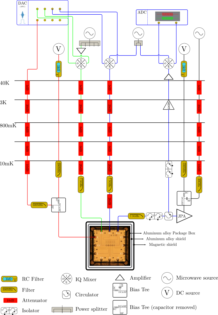
The schematic diagram of our experimental setup is shown in Supplementary Figure S1. The measurement platform contains XY lines ( green line), Z control lines (red line), and readout line (blue line). The more details of measurement platform is presented in the Methods. The device photo is shown on the bottom of Supplementary Figure S1 and the corresponding device parameters are presented in Supplementary Table. 1.
II.2 Readout calibration
JPA Mutus is used to improve the signal to noise ratio (SNR) of readout signals, and its gain curve is shown in Supplementary Figure S2. The duration time of our readout pulse is 2 . The transmission data corresponding to five readout resonators are shown, respectively, in the upper row of Supplementary Figure S3. IQ data at specified frequency values (as indicated by black arrows) are shown in the lower row of Supplementary Figure S3. Blue (orange) lines or dots represent data when qubits are prepared at state (). There are 2000 dots (repetitions) for each statistic. The readout fidelity and of are listed in Supplementary Table 1.
II.3 Coherence time
Values of energy relaxation time and dephasing time for 5 qubits at their idle frequencies are listed in Supplementary Table 1. The corresponding temporal results are shown in Supplementary Figure S4. We also measure of all 5 qubits around working frequency 4.868 GHz, where the working points of our experiments are in this frequency interval, see Supplementary Figure S5. The energy relaxation time is long enough to ensure that all 5 qubits have acceptable coherence performance.


II.4 Z control line crosstalk
Each qubit is tuned by current pulses applied to its Z control line. However, there are crosstalks between Z control lines, which means that the current pulse on one Z control line can also affect other qubits. To evaluate the influence of such crosstalk, we bias target qubit at which is more than 1 GHz below its maximum frequency, so that the qubit frequency is sensitive to external magnetic flux as well as the Z pulse crosstalk. We apply a long () Gaussian shaped resonant X () pulse, and then measure the excitation probability of . Applying a Z pulse with amplitude to the Z control line of another qubit will generate a crosstalk pulse on , as shown in Supplementary Figure S6. Such a crosstalk pulse would lead to a frequency change for , and hence the decrease of the excitation probability. We apply a compensation pulse with amplitude to the Z control line of to cancel this crosstalk. In practice, we monitor the excitation probability as a function of compensation pulse amplitude. When a complete compensation is achieved, the excitation probability is maximized. The linear relation between and is shown in Supplementary Figure S7.


After completing such crosstalk-compensation measurement for all qubits, a full transformation matrix for Z control line crosstalk calibration is constructed and shown in Eq.S1, where represents the actual amplitude applied on the Z control line of , and represents the effective amplitude after taking crosstalk compensation into account.
| (S1) |
II.5 Calibration of time delay for all control channels
To guarantee the pulses applied on different control channels reaching to chip at the expected time, the output delay time of AWG ports need to be adjusted to compensate the transmission time difference in different channels. In our experiment, we set Z control channel of as the reference, and make all other control channels align to it. There are two steps: In the first step, we align Z control channels by aligning to , followed by to and so forth. In the second step, we align XY control channel of each qubit to its Z control channel.
Scheme for determining Z control channel delay length is shown in Supplementary Figure S8. The blue lines represent transmission time in control channels. The red lines are the output delays that we insert before AWG output. The black dots are the AWG output start times. By adjusting the length of output delay, we can make the Z pulses align to the reference channel. In experiment, we set (or ) to , then apply two square pulses to make and resonantly coupled for a time duration . This means that if two pulses are aligned, the resonant coupling will induce a complete photon swap. Here is the coupling strength between and . During the measurement, we vary the length of output delay time of and measure (or ) after the Z pulses. The final state of (or ) depends on the overlap of two Z pulses. When two pulses are aligned, the overlap will be equal to , and the swap probability will be the highest. The experimental results and fittings are shown in Supplementary Figure S10. In our experimental setup, the cables connecting qubits and electronics are designed to be of the same length, so the final adjustment of the output delay is in the range of ps.
After the alignment of all Z control channels, we align XY control channel of each qubit to its Z control channel in time. As shown in Supplementary Figure S9, the effective excitation probability of is the integral of Gaussian shaped pulse over time before the Z pulse. When we adjust the output delay of XY channel, and measure the final state of , we obtain the data in Supplementary Figure S11. By fitting the data, we can get the proper output delay time of XY channel. With cables of the same length, the measured delay times are also small and in the range of ps.
II.6 Square pulse distortion correction
In our experiment, qubits are tuned to specified frequencies by square pulses. However, an ideal square pulse is usually distorted when reaching to the chip. To correct this distortion, we need to determine the deformed shape of the step edge of Z square pulse. The corresponding qubit is biased to a relative low frequency (more than 1GHz below its maximum frequency) to improve its sensitivity to the pulse shape deformation. As shown in Supplementary Figure S12, an amplitude fixed () step signal is applied to a qubit, and followed a pulse with frequency and length 20ns. If there is no distortion, the qubit will be excited to by the pulse. If there is small distortion after the step signal, qubit will not be completely excited to . By varying the compensation amplitude , we can find the value of full compensation when the maximum excitation probability is achieved. By changing the delay time of pulse, we can get a view of the distorted step signal response, as shown in the upper row of Supplementary Figure S13. With this response data, we can calculate the needed adjustments for the square pulses. Then, we repeat the measurement in Supplementary Figure S12 with corrected pulses , and find the step signal response is flattened, see the lower row of Supplementary Figure S13.
II.7 Calibration of initial state phase
In order to measure the energy density transport, we need to prepare 5 qubits in an initial state such as , and measure the expectation value of correlated operator (). In the experiment, we firstly rotate and to X-Y plane with a pulse and set the initial state of as , then we need to adjust the state of by changing the phase of pulse to make at , see Supplementary Figure S14. Here, we use the Bloch sphere representation for describing the state of a qubit. Then these two qubits are resonantly coupled to each other at the frequency . (In our experiment, we need to resonantly couple all 5 qubits at this frequency, and set a linear frequency gradient around .) After time , we measure the final state probability as a function of the phase . The corresponding result is shown in the leftmost figure in Supplementary Figure S15. The curves of and are consistent with theoretical and numerical analysis. The cross point, indicated by the black arrow, corresponds to the when the state of is also . In a similar way, we can calibrate the phase between and , and so forth.
II.8 Calibration of dynamical phase
To measure the expectation value of correlated operator (), we need to determine the phase of final state for each qubit. In our experiment, qubits are coupled at frequency , but are rotated and measured at their individual idle frequencies . The frequency difference between and can lead to a dynamical phase accumulation to the final state. Thus, in our experiment, we need to calibrate this accumulated dynamical phase.
The accumulation of the dynamical phase can be divided into three parts: rising edge part, middle flat part, and falling edge part. The summation, represented by the shadowed part in Supplementary Figure S16, can be expressed as . Due to the presence of the rising and falling edges, the actual dynamical phase accumulation, comparing with , has an approximately fixed offset . To determine , we use the Ramsey-like method as shown in Supplementary Figure S16. The phase of the first pulse is and fixed, and the phase of the second pulse is . Thus, when , the phase of the second pulse is equivalent to , and the qubit will be in .
The calibrated results of , , , and are shown in Supplementary Figure S17.


III Supplementary Note 2. Wannier-Stark Localization Length
Here, by Jordan-Wigger transformation, the Hamiltonian (2) can be mapped to a free-fermion lattice model
| (S2) |
where () is the fermion creation (annihilation) operator. Here, without loss of generality, we consider is site-independent, i.e., . Under a linear potential, i.e., , the system can exhibit Wannier-Stark localization with localization length Dahan1996. This localization length can be understood classically as following Dahan1996: For a single particle, it can have the maximum kinetic energy . In addition, the particle need to consume the kinetic energy when hopping to the next site due to the linear potential. Thus, the maximum distance that a particle can propagate is about , i.e., Wannier-Stark localization length.
For a finite-size system, similarly, due to the linear potential, the particle cannot propagate completely from one boundary to another. In this picture, we can find that the maximum probability of a particle propagating from one boundary to another (i.e., in the main text.) can indeed reflect the localization length. We assume that the localized wavefunction has the form
| (S3) |
where is a normalized factor, represents that the wave function is localized at site , is the vacuum state of . Therefore, intuitively, we expect that the maximum probability of a particle propagating from one boundary to another is proportional to , where is the corresponding factor. In Supplementary Figure S18, we present the numerical result of the relation between and , and we can find that with .
IV Supplementary Note 3. Spin Current
In this section, we consider the spin current under the linear potential. The spin current of Hamiltonian (2) can be defined as
| (S4) |
where represents the -th bond of the chain. It can also be measured in our platform by the joint readout of two nearest-neighbor qubits. Here, we present the numerical results [see Supplementary Figure S19]. When , the spin current has nearly no decay as the increase of the propagation distance, while it decays quickly for . Thus, this behavior of spin currents is an another signature of Wannier-Stark localization.

References
- (1) J. Y. Mutus, T. C. White, R. Barends, Yu Chen, Z. Chen, B. Chiaro, A. Dunsworth, E. Jeffrey, J. Kelly, A. Megrant, C. Neill, P. J. J. O’Malley, P. Roushan, D. Sank, A. Vainsencher, J. Wenner, K. M. Sundqvist, A. N. Cleland, and John M. Martinis, Strong environmental coupling in a Josephson parametric amplifier, Appl. Phys. Lett. 104, 263513 (2014).
- (2) M. Ben Dahan, E. Peik, J. Reichel, Y. Castin, and C. Salomon, Bloch oscillations of atoms in an optical potential, Phys. Rev. Lett. 76, 4508 (1996).