A Hölderian backtracking method for min-max and min-min problems

Jérôme Bolte Thanks: Authors are listed in alphabetical order Affiliation: Toulouse School of Economics Affiliation: University of Toulouse Email: jerome.bolte@ut-capitole.fr Lilian Glaudin Note: Affiliation: ANITI Affiliation: University of Toulouse Email: lilian@glaudin.net Edouard Pauwels Note: Affiliation: IRIT Affiliation: Unversity of Toulouse Email: edouard.pauwels@irit.fr Mathieu Serrurier Note: Affiliation: IRIT Affiliation: University of Toulouse Email: mathieu.serrurier@irit.fr

Abstract

We present a new algorithm to solve min-max or min-min problems out of the convex world. We use rigidity assumptions, ubiquitous in learning, making our method applicable to many optimization problems. Our approach takes advantage of hidden regularity properties and allows us to devise a simple algorithm of ridge type. An original feature of our method is to come with automatic step size adaptation which departs from the usual overly cautious backtracking methods. In a general framework, we provide convergence theoretical guarantees and rates. We apply our findings on simple GAN problems obtaining promising numerical results.

1 Introduction

Adversarial learning, introduced in [18], see also [2], calls for the development of algorithms addressing large scale, smooth problems of the type

\displaystyle\min_{x\in\mathbb{R}^{d}}\max_{y\in{\mathcal{Y}}}L(x,y),

(1.1)

where ${\mathcal{Y}}$ is a constraint set, and $L$ is a given cost function. This structure happens to be ubiquitous in optimization and game theory, but generally under assumptions that are not those met in learning. In optimization it stems from the Lagrangian approach and duality theory, see e.g., [10, 6, 12], while in game theory it comes from zero-sum 2-players games, see e.g., [35, 36, 24]. Dynamics for addressing (1.1) have thus naturally two types. They may be built on strategic considerations, so that algorithms correspond to a sequence of actions chosen by antagonistic players, see [24] and references therein. In general these methods are not favorable to optimization because the contradictory interests of players induce oscillations and slowness in the identification of optimal strategies. Optimization algorithms seem more interesting for our purposes because they focus on the final result, i.e., finding an optimal choice $x$ , regardless of the adversarial strategy issues. In that respect, there are two possibilities: the variational inequality approach which treat minimization and maximization variables on an equal footing, see e.g. [22, 27, 12] or [26, 21, 17] in learning. On the other hand, some methods break this symmetry, as primal or augmented Lagrangian methods. In those, a large number of explicit steps, implicit steps, or global minimization are performed on one variable while the other is updated much more cautiously in an explicit incremental way, see e.g., [6, 33].

Our work is written in this spirit: we assume that the under-max argument is tractable with a good precision, and we construct our algorithm on the following model:

		$\displaystyle y_{n}=\text{\rm argmax}\,_{y\in{\mathcal{Y}}}L(x_{n},y),$
		$\displaystyle x_{n+1}=x_{n}-\gamma_{n}\nabla_{x}L(x_{n},y_{n}),\gamma_{n}>0,\,n\geq 0.$

As explained above, the rationale is not new¹¹ 1 It can be traced back to the origin of augmented Lagrangian methods, see e.g., [31], and is akin to many methods in the literature on learning where the global optimization is performed approximately by multiple gradient steps [29, 30] or by clever revision steps, as in the "follow the ridge" method, see [37].

Backtrack Hölder

What is new then? The surprising fact is that we can provide theoretical grounds to devise large steps and thus obtain aggressive learning rates with few assumptions. This is done by exploiting some hidden properties of the value function $g=\max_{y}L(\cdot,y)$ under widespread rigidity assumptions. Let us sketch the ideas of our approach. First, under a uniqueness assumption on the maximizer, our method appears to be a gradient method on the value function for “player I" ( “the generator" of GANs)

x_{n+1}=x_{n}-\gamma_{n}\nabla g(x_{n}).

Secondly, we use the fact that $g$ has a locally Hölderian gradient²² 2 Recall that $G\colon\mathbb{R}^{d}\mapsto\mathbb{R}^{d^{\prime}}$ is locally Hölderian if for all bounded subset $V\subset\mathbb{R}^{d}$ , there exists $\beta$ and $\nu$ positive such that $\|G(x)-G(y)\|\leq\beta\|x-y\|^{\nu}$ , whenever $x,y\in V$ . whenever $L$ is semi-algebraic or analytic-like, a situation which covers most of the problems met in practice. With such observations, we may then develop automatic learning rate strategies and a diagonal backtracking method, that we call “Backtrack Hölder methods for min-max".

Contributions

•

We provide new algorithms whose steps are tuned automatically: Backtrack Hölder gradient and Backtrack Hölder for min-max methods.
•

Our algorithms are shown to perform with $O(\epsilon^{-[2+c]})$ rate, where $c$ is a cost incurred by the diagonal backtracking process (which is negligible in practice), and to provide general convergence guarantees to points $(x^{*},y^{*})$ satisfying $y^{*}=\text{\rm argmax}\,_{y}L(x^{*},y)$ and $\nabla_{x}L(x^{*},y^{*})=0$ . This is done within a fairly general framework, since $L$ is merely assumed semi-algebraic while the “best response" of player II is only required to be singled-valued.
•

A byproduct of our work is a global convergence result for Hölder methods, which were earlier investigated in the literature [5, 19, 28, 38].
•

Our work is theoretical in essence. It is merely a first step towards more involved research, regarding the effect of nonsmoothness or stochastic subsampling. We propose however numerical experiments on learning problems. First on the “Sinkhorn GANs", [16, 15], which rely on optimal transport losses regularized through the addition of an entropic term, and second on Wasserstein GANs [2] which are a natural extensions of GANs [18].

2 Gradient algorithms à la Hölder

Our results often use semi-algebraic assumptions which are pervasive in optimization and machine learning, see e.g. [11] and references therein.

Our method and proofs are presented in view of solving min-max problems, but the techniques are identical for the min-min case. $\mathbb{R}^{d},\mathbb{R}^{d^{\prime}}$ are endowed with their Euclidean structure.

2.1 Framework: a single valued best response and semi-algebraicity

Let ${\mathcal{Y}}\subset\mathbb{R}^{d^{\prime}}$ be a nonempty closed semi-algebraic set, see Definition A.1 in Appendix.

Properties of the value function and its best response

Assumption 2.1 (Standing assumptions)

$L$ is a $C^{1}$ semi-algebraic function on $\mathbb{R}^{d}\times\mathbb{R}^{d^{\prime}}$ such that $(x,y)\mapsto\nabla_{x}L(x,y)$ is jointly continuous. Furthermore, for any compact sets $K_{1}\subset\mathbb{R}^{d}$ and $K_{2}\subset\mathbb{R}^{d^{\prime}}$ , there exist $\beta_{1},\beta_{2}\in\left]0,+\infty\right[$ such that, $\forall x_{1},x_{2}\in K_{1},\,\forall y_{1},y_{2}\in K_{2},$

\|\nabla_{x}L(x_{1},y_{1})-\nabla_{x}L(x_{2},y_{2})\|\leq\beta_{1}\|x_{1}-x_{2}\|+\beta_{2}\|y_{1}-y_{2}\|.

(2.1)

Borrowing the terminology from game theory, one defines the value function as $g(\cdot)=\max_{y\in{\mathcal{Y}}}L(\cdot,y)$ and the best response mapping $p(\cdot)=\text{\rm argmax}\,_{y\in{\mathcal{Y}}}L(\cdot,y)$ for $x\in\mathbb{R}^{d}$ .

Assumption 2.2 (Well posedness)

H1. $p(x)$ is nonempty and single valued for every $x\in\mathbb{R}^{d}$ ,
H2. $p$ is continuous.

The first part of the assumption is satisfied whenever $L(x,\cdot)$ is strictly concave, see e.g. [25]. Note also that if $L(x,\cdot)$ is concave, as in a dual optimal transport formulation, some regularization techniques can be used to obtain uniqueness and preserve semi-algebraicity, see e.g., [14]. As for the H2 continuity assumption, it is much less stringent than it may look:

Proposition 2.3 (Continuity of $p$ )

Suppose that Assumption 2.1 and Assumption 2.2-H1 are satisfied, and that either ${\mathcal{Y}}$ is compact, or $p$ is bounded on bounded sets. Then the best response $p$ is a continuous function, that is Assumption 2.2-H2 is fulfilled.

Combining these assumptions with Tarski-Seidenberg theorem and the properties of semi-algebraic functions [7], we obtain the following.

Proposition 2.4 (Properties of $p$ and $g$ )

Suppose that Assumption 2.1 and Assumption 2.2 are satisfied. Then

(i)

$g$ is differentiable and for all $\bar{x}\in\mathbb{R}^{d}$ , $\nabla g(\bar{x})=\nabla_{x}L(\bar{x},p(\bar{x}))$ ,
(ii)

both the value function $g$ and the best response $p$ are semi-algebraic,
(iii)

the gradient of the value function, $\nabla g$ , is locally Hölder.

Remark 2.5

Consider $L(x,y)=xy$ , ${\mathcal{Y}}=[-1,1]$ , one sees that $g(x)=\max_{y\in[-1,1]}L(x,y)=|x|$ while $p(x)=\mbox{sign }x$ if $x\neq 0$ and $p(0)=[-1,1]$ . This shows that Assumption 2.2 is a necessary assumption for $g$ to be differentiable. One cannot hope in general for $\nabla g$ to be locally Lipschitz continuous. For instance set ${\mathcal{Y}}=\mathbb{R}_{+}$ , $L(x,y)=xy-\frac{1}{3}y^{3}$ , then $g(x)=\max_{y\in\mathbb{R}^{+}}L(x,y)=\frac{2}{3}x^{3/2}$ with $\nabla g(x)=\sqrt{x}$ .

Comments and rationale of the method

At this stage the principles of our strategy can be made precise. We deal with problems which are dissymetric in structure: the argmax is easily computable or approximable while the block involving the minimizing variable is difficult to handle. This suggests to proceed as follows: one computes a best response mapping (even approximately), the gradient of the value function becomes accessible via formula (i) in Proposition 2.4, and thus a descent step can be taken. The questions are: which steps are acceptable? Can they be tuned automatically? This is the object of the next sections.

2.2 Gradient descent for nonconvex functions with globally Hölderian gradient

The results of this section are self contained. We consider first the ideal case of a gradient method on a globally Hölder function with known constants, see e.g. [28, 38]. We study Algorithm 2, previously presented in [38] for which we prove sequential convergence.

Assumption 2.6 (Global Hölder regularity)

$f\colon\mathbb{R}^{d}\to\mathbb{R}$ is $C^{1}$ , semi-algebraic and

\forall x_{1},x_{2}\in\mathbb{R}^{d},\,\quad\|\nabla f(x_{1})-\nabla f(x_{2})\|\leq\beta\|x_{1}-x_{2}\|^{\nu},\mbox{ with }\beta>0,\,\nu\in]0,1].

(2.2)

Input:

\nu\in\left]0,1\right]

\beta\in\left]0,+\infty\right[

and

\gamma\in]0,(\nu+1)/\beta[

Initialization :

x_{0}\in\mathbb{R}^{d}

for $n=0,1,\ldots$ do

\gamma_{n}(x_{n})=\gamma\left(\frac{\nu+1}{\beta}\right)^{1/\nu-1}\|\nabla f(x_{n})\|^{1/\nu-1}

x_{n+1}=x_{n}-\gamma_{n}(x_{n})\nabla f(x_{n})

Algorithm 1 Hölder gradient method

Proposition 2.7 (Convergence of the Hölder gradient method for nonconvex functions)

Under Assumption 2.6, consider a bounded sequence $(x_{n})_{n\in\mathbb{N}}$ generated by Algorithm 1. Then the following hold:

(i)

the sequence $(f(x_{n}))_{n\in\mathbb{N}}$ is nonincreasing and converges,
(ii)

the sequence $(x_{n})_{n\in\mathbb{N}}$ converges to a critical point $x^{*}\in\mathbb{R}^{d}$ of $f$ , i.e., $\nabla f(x^{*})=0$ ,

(iii)

for every $n\in\mathbb{N}$ ³³ 3 This result is essentially present in [38],

\min_{0\leq k\leq n}\|\nabla f(x_{k})\|^{\frac{1}{\nu}+1}\leq\left[\frac{f(x_{0})-f(x^{*})}{\gamma-\gamma^{\nu+1}\left(\frac{\beta}{\nu+1}\right)^{\nu}}\left(\frac{\beta}{\nu+1}\right)^{\frac{1-\nu}{\nu}}\right]\dfrac{1}{n+1}=O\left(\frac{1}{n}\right).

Choosing $\gamma=\frac{\nu+1}{\beta}\left(\frac{1}{\nu+1}\right)^{1/\nu}$ , we obtain

\min_{0\leq k\leq n}\|\nabla f(x_{k})\|^{\frac{1}{\nu}+1}\leq\frac{(f(x)-f(x^{*}))\beta^{1/\nu}(\nu+1)}{\nu(n+1)}.

2.3 The “Backtrack Hölder” gradient algorithm and diagonal backtracking

In practice, the constants are unknown and the Hölderian properties are merely local. The algorithm we present now (Algorithm 2), is in the spirit of the classical backtracking method, see e.g., [6]. The major difference is that we devise a diagonal backtracking, to detect both constants $\beta,\nu$ at once in a single searching pass.

Assumption 2.8

$f\colon\mathbb{R}^{d}\to\mathbb{R}$ is a $C^{1}$ semi-algebraic function such that $\nabla f$ is locally Hölder.

In the following algorithm, $\alpha,\gamma>0$ are step length parameters, $\delta>0$ is a sufficient-decrease threshold and $\rho>0$ balances the search between the unknown exponent $\nu$ and the unknown multiplicative constant $\beta$ , see Assumption 2.6.

Input:

\delta,\alpha\in\left]0,1\right[

and

\gamma,\rho\in\left]0,+\infty\right[

Initialization :

x_{0}\in\mathbb{R}^{d}

k_{-1}=0

for $n=0,1,\ldots$ do

k=k_{n-1}

\gamma_{n}(x_{n})=\alpha^{k}\min\{1,\|\nabla f(x_{n})\|^{\rho k}\}\gamma

while $f(x_{n}-\gamma_{n}(x_{n})\nabla f(x_{n}))>f(x_{n})-\delta\gamma_{n}(x_{n})\|\nabla f(x_{n})\|^{2}$ do

k=k+1

\gamma_{n}(x_{n})=\alpha^{k}\min\{1,\|\nabla f(x_{n})\|^{\rho k}\}\gamma

k_{n}=k

x_{n+1}=x_{n}-\gamma_{n}(x_{n})\nabla f(x_{n})

Algorithm 2 Backtrack Hölder gradient method

The following theorem provides convergence guarantees under local Hölder continuity (Assumption 2.8 for Algorithm 2).

Theorem 2.9 (Convergence of Backtrack Hölder for nonconvex functions)

Under Assumption 2.8, consider a bounded sequence $(x_{n})_{n\in\mathbb{N}}$ generated by Algorithm 2. Then the following hold:

(i)

$(\gamma_{n})_{n\in\mathbb{N}}$ is well defined,
(ii)

the sequence $(f(x_{n}))_{n\in\mathbb{N}}$ is nonincreasing and converges,
(iii)

there exists $x^{*}\in\mathbb{R}^{d}$ such that $x_{n}\to x^{*}$ and $\nabla f(x^{*})=0,$
(iv)

the while loop has a uniform finite bound $\bar{k}:=\sup_{n\in\mathbb{N}}k_{n}<{+\infty}$ . Moreover

$\min_{0\leq i\leq n}\|\nabla f(x_{i})\|=O\left(\frac{1}{n^{\frac{1}{2+\rho\bar{k}}}}\right),$

(v)

suppose moreover that there exist $\beta\in\left]0,+\infty\right[$ and $\nu\in]0,1]$ such that $\nabla f$ is globally $(\beta,\nu)$ Hölder. Then

\sup_{n\in\mathbb{N}}k_{n}\leq 1+\frac{1}{\nu}\max\left\{\frac{\log\left(\frac{(1-\delta)(\nu+1)}{\gamma^{\nu}\beta}\right)}{\log(\alpha)},\frac{1-\nu}{\rho}\right\}.

(2.3)

Remark 2.10 (Diagonal backtracking alternatives and comments)

In the previous theorem, we ask $(k_{n})_{n\in\mathbb{N}}$ to be a nondecreasing sequence and (2.3) is actually a bound on the total number of additional calls to the function in the while loop. In practice, this approach might be too conservative and other strategies may provide much more aggressive steps at the cost of additional calls to the function. We will use two variations to update $(k_{n})_{n\in\mathbb{N}}$ :

•

Initialize $k$ to $0$ for fine tuning to the price of longer inner loops (see Algorithm 8).
•

For some iterations, decrease the value of $k$ by $1$ (see Algorithm 5 for example).

The parameters $\alpha,\gamma,\delta$ , and $\rho$ are made to tune finely the number of iterations spent on estimating local Hölder constants.

In Theorem 2.9 (v), we need to suppose that the gradient is globally Hölder contrary to Assumption 2.8.

3 Backtrack Hölder for min-max problems

Gathering the results provided in Section 2.3, we provide here our main algorithm (Algorithm 3).

Input:

\delta,\alpha\in\left]0,1\right[

and

\gamma,\rho\in\left]0,+\infty\right[

Initialization :

x_{0}\in\mathbb{R}^{d}

y_{0}=\arg\max_{z\in\mathcal{Y}}L(x_{0},z)

k_{-1}=0

for $n=0,1,\ldots$ do

k=k_{n-1}

\gamma_{n}(x_{n})=\gamma\alpha^{k}\min\{1,\|\nabla_{x}L(x_{n},y_{n})\|^{\rho k}\}

x=x_{n}-\gamma_{n}(x_{n})\nabla_{x}L(x_{n},y_{n})

y=\arg\max_{z\in\mathcal{Y}}L(x,z)

while $L(x,y)>L(x_{n},y_{n})-\delta\gamma_{n}(x_{n})\|\nabla_{x}L(x_{n},y_{n})\|^{2}$ do

k=k+1

\gamma_{n}(x_{n})=\gamma\alpha^{k}\min\{1,\|\nabla_{x}L(x_{n},y_{n})\|^{\rho k}\}

x=x_{n}-\gamma_{n}(x_{n})\nabla_{x}L(x_{n},y_{n})

y=\arg\max_{z\in\mathcal{X}}L(x,z)

k_{n}=k

x_{n+1}=x

y_{n+1}=y

Algorithm 3 Monotone Backtrack Hölder for min-max

Several comments are in order:

— The above contains an inner loop whose overhead cost becomes negligible as $n\to\infty$ , this allows one for automatic step size tuning. The form of Algorithm 3 is slightly different from Algorithm 2 to avoid duplicate calls to the max-oracle required both to compute gradients and evaluate functions.

— As described in Remark 2.10, the backtracking strategy is one among others and it is adaptable to different settings. In this min-max case, the cost of the max-oracle may have some impact: either it is costly and extra-flexibility is needed or it is cheap and it can be kept as is. Two examples are provided in Sections 4.1 and 4.2.

— A direct modification of the above method, provides also an algorithm for

\min_{x\in\mathbb{R}^{d}}\min_{y\in{\mathcal{Y}}}L(x,y).

(3.1)

— Algorithm 3 is a model algorithm corresponding to a monotone backtracking approach (i.e., the sequence $(k_{n})$ is nondecreasing), but many other variants are possible, see Appendix D. Algorithms 5 and 6 are for the min-min problem, with a non monotone backtracking and the same guarantees. A heuristic version is also considered: it is Algorithm 8 where an approximation of the argmax is used.

To benchmark our algorithms, we compare them to Algorithms 4, 6, and 7 in Appendix D, with constant but finely tuned step sizes or with Armijo search.

Theorem 3.1 (Backtrack Hölder for min-max)

Under Assumptions 2.1 and 2.2, consider the sequences $(x_{n})_{n\in\mathbb{N}}$ and $(y_{n})_{n\in\mathbb{N}}$ generated by Algorithm 3. Suppose that $(x_{n})_{n\in\mathbb{N}}$ is bounded. Then

(i)

The while loop has a uniform bound, i.e., $\sup_{n\in\mathbb{N}}k_{n}<{+\infty}$ .
(ii)

$(x_{n})_{n\in\mathbb{N}}$ converges to $x^{*}$ in $\mathbb{R}^{d}$ and $(y_{n})_{n\in\mathbb{N}}$ converges to $y^{*}\in{\mathcal{Y}}$ , with $\nabla_{x}L(x^{*},y^{*})=0$ and $y^{*}=\text{\rm argmax}\,_{y\in{\mathcal{Y}}}L(x^{*},y)$ .

(iii)

Suppose that there exist $\beta\in\left]0,+\infty\right[$ and $\nu\in]0,1]$ such that $\nabla g$ is $(\beta,\nu)$ Hölder everywhere. Then the cost of the while loop is bounded by

\displaystyle\sup_{n\in\mathbb{N}}k_{n}\leq 1+\frac{1}{\nu}\max\left\{\frac{\log\left(\frac{(1-\delta)(\nu+1)}{\gamma^{\nu}\beta}\right)}{\log(\alpha)},\frac{1-\nu}{\rho}\right\}.

(3.2)

Remark 3.2

In [18, Proposition 2], the authors mention an algorithm akin to what we proposed, but without backtracking. They insist on the fact that if one had access to the max-oracle, then one would be able to implement a gradient descent by using "sufficiently small updates". Our theoretical results are an answer to this comment as we offer a quantitative characterization of how small the step should be, as well as a backtracking estimation technique.

4 Numerical experiments

We compare our method with constant step size algorithm and Armijo backtracking for the Generative Adversarial Network (GAN) problem, first using Sinkhorn divergences and second considering Wasserstein adversarial networks. 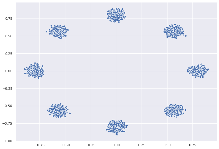Data lie in $\mathbb{R}^{d}=\mathbb{R}^{2}$ , the sample size is $N=1024$ and we consider $x_{1},\ldots,x_{N}\in\mathbb{R}^{d}$ a fixed sample from a distribution $\mathbb{P}_{d}$ , which is a Gaussian mixture, see Figure 1, and $z_{1},\ldots,z_{N}\in\mathcal{Z}$ a fixed sample from latent distribution $\mathbb{P}_{z}=U([0,1]\times[0,1])$ , uniform on $\mathcal{Z}$ , where $\mathcal{Z}=[0,1]\times[0,1]$ .

Refer to caption — Figure 1: Data distribution $x_{1},\ldots,x_{N}$

We consider as generator $G$ , a dense neural network with three hidden layers containing respectively $64$ , $32$ , $16$ neurons with a ReLU activation between each layer. We write $G:\mathcal{Z}\times\Theta_{G}\to\mathcal{X}$ , with inputs in $\mathcal{Z}$ and parameters $\theta_{G}\in\Theta_{G}$ where $\Theta_{G}=\mathbb{R}^{q}$ with $q$ the total number of parameters of the network (2834 in our case).

4.1 Sinkhorn GAN

We first consider training generative network using Sinkhorn divergences as proposed in [16]. This is a min-min problem which satisfies Assumption 2.2 (see also the remark in Equation 3.1). Sinkhorn algorithm [34, 14] allows us to compute a very precise approximation of the min-oracle required by our algorithm, we use it as an exact estimate. Note that the transport plan for the Sinkhorn divergence is regularized by an entropy term whence the inner minimization problem has a unique solution and the corresponding $p$ is continuous. This is a perfect example to illustrate our ideas. Consider the following probability measures

	$\displaystyle\bar{\mu}$	$\displaystyle=\frac{1}{N}\sum_{i=1}^{N}\delta_{x_{i}},$	$\displaystyle\text{(empirical target distribution)},$
	$\displaystyle\mu(\theta_{G})$	$\displaystyle=\frac{1}{N}\sum_{i=1}^{N}\delta_{G(z_{i},\theta_{G})},$	$\displaystyle\text{(empirical generator distribution)}.$

We then define the Sinkhorn divergence between these two distributions.

\displaystyle\mathcal{W}_{\epsilon}(\bar{\mu},\mu(\theta_{G}))

\displaystyle=\min_{P\in\mathbb{R}_{+}^{N\times N}}\left\{\mbox{Tr}(PC(\theta_{G})^{T})+\epsilon\sum_{i,j=1}^{N}P_{ij}\log(P_{ij})\;;\;P1_{N}=1_{N},P^{T}1_{N}=1_{N}\right\}

where $\epsilon>0$ is a regularization parameter, $\displaystyle C(\theta_{G})=\left[\|G(z_{i},\theta_{G})-x_{j}\|\right]_{i,j}\in\mathbb{R}^{N\times N}$ is the pairwise distance matrix between target observations $(x_{i})_{1\leq i\leq N}$ and generated observations $(G(z_{i},\theta_{G}))_{1\leq i\leq N}$ . Here Tr is the trace, and $1_{N}$ is the all-ones vector. The optimum is unique thanks to the entropic regularization and the optimal transportation plan $P$ can be efficiently estimated with an arbitrary precision by Sinkhorn algorithm [34, 14].

Training our generative network amounts to solving the following min-min problem

\min_{\theta_{G}}\mathcal{W}_{\epsilon}(\bar{\mu},\mu(\theta_{G})).

Remark 4.1 (Global subanalyticity ensures Łojasiewicz inequality)

The cost function of the Sinkhorn GAN problem is not semi-algebraic due to log. However we never use the logarithm in a neighborhood of $0$ during the optimization process because of its infinite slope. Hence the loss can actually be seen as globally subanalytic. Whence $p$ , $g$ are globally subanalytic and the Łojasiewicz inequality as well as Hölder properties still hold, see [7, 3, 9] for more on this.

Algorithmic strategies for Sinkhorn GAN

The monotone diagonal backtracking is too conservative for this case, so we use a variant described in Algorithm 5 instead. At each step, the idea is to try to decrease $k$ of $1$ whenever possible, keeping some sufficient-decrease property valid. Otherwise $k$ is increased as in the monotone method, until sufficient decrease of the value is ensured. This approach is particularly adapted to the Sinkhorn case, because estimating the best response is cheap.

Note that, to propose a fair comparison and keep the same complexity between algorithms, we count each call to the min-oracle, both in the outer and in the inner while loop, as an iteration step. The parameters used in this experiment for Algorithm 5 are $\gamma=1$ , $\alpha=0.5$ , $\delta=0.25$ , $\delta_{+}=0.95$ , and $\rho=0.5$ . We compare with Algorithm 4 presented in Appendix D, which is a constant step size variant, we try with different step size parameters $\gamma\in\{0.01,0.05,0.1\}$ . We compare with the standard Armijo backtracking algorithm (see Algorithm 6 in Appendix D) which uses a similar approach as in Algorithm 5 to tune the step size parameter $\gamma_{n}$ , but does not take advantage of the Hölder property. All algorithms are initialized randomly with the same seed.

We observe on the left part of Figure 2 that both Hölder and Armijo backtracking provide decreasing sequence and avoid oscillations. Both algorithms converge faster than the constant step size variant. Furthermore, since our algorithm can take into account the norm of the gradient, the number of intern loop is smaller and that explain why the Non Monotone Hölder backtracking is faster.

4.2 Wasserstein GAN

We treat the Wasserstein GAN (WGAN) heuristically with an approximation of the max-oracle and use Algorithm 8 in Appendix D which matches this setting.

Consider a second neural network, called discriminator, $D:\mathbb{R}^{d}\times\Theta_{D}\to\mathbb{R}$ with inputs in $\mathbb{R}^{d}$ and parameters $\theta_{D}\in\Theta_{D}$ whose architecture is the same as $G$ (i.e., $\Theta_{D}=\Theta_{G}$ ) but with a fullsort activation between each layer, see [1]. We consider the following problem

\min_{\theta_{G}}\max_{\theta_{D}}\sum_{i=1}^{n}D(x_{i},\theta_{D})-\sum_{j=1}^{n}D(G(z_{j},\theta_{G}),\theta_{D}).

In order to implement the analogy with Kantorovitch duality in the context of GANs [2], one has to ensure that the discriminator $D$ is 1-Lipschitz, when seen as a function of its input neurons. This is enforced using a specific architecture for the discrimintator network $D$ . We use Bjork orthonormalization and fullsort activation functions [1] which ensure that the network is $1$ -Lipschitz without any restriction on its weight parameters $\theta_{D}$ .

For this problem, we use Algorithm 8, which is a heuristic modification of our method designed to deal with the inner max. Both the argmax and max are indeed approximated by gradient ascent. Algorithm 8 then implements the same bactracking idea which is evaluated on the same to benchmark as in the previous section. Extra discussions are provided in the Appendix. Doing so, the extra-cost induced by the while loop becomes negligible and we can find the optimal value of $k$ by exhaustive search. For this reason, in this heuristic context, Hölder backtracking schemes have very little advantage compared to Armijo and we do not report comparison. Detailed investigations for large scale networks is postponed to future research. Since GAN’s training is delicate in practice [20], we provide comparison with many step size choices for the constant step size algorithm. Algorithm 7 that the difference between Armijo method and ours As for Backtrack Hölder min-max, we use parameters $\gamma=1$ , $\delta=0.75$ , $\alpha=0.75$ , and $\rho=0.20$ for the Hölder backtracking algorithm and constant step size parameter $\gamma\in\{0.001,0.01,0.05,0.1,0.5\}$ for the constant step size variant. All algorithms are initialized randomly with the same seed.

Figure 2 displays our results on the right. The optimal loss equals $0$ . One observes that constant large steps are extremely oscillatory while small steps are stable but extremely slow. Backtrack Hölder takes the best of the two world, oscillates much less and stabilizes closer to the optimal loss value compared to constant step size variants.

Broader impact

The authors think that this work is essentially theoretical and that this section does not apply.

Acknowledgements. The authors acknowledge the support of ANR-3IA Artificial and Natural Intelligence Toulouse Institute. JB and EP thank Air Force Office of Scientific Research, Air Force Material Command, USAF, under grant numbers FA9550-19-1-7026, FA9550-18-1-0226, and ANR MasDol. JB acknowledges the support of ANR Chess, grant ANR-17-EURE-0010 and ANR OMS.

References

[1] Cem Anil, James Lucas, and Roger Grosse. Sorting out Lipschitz function approximation. In Kamalika Chaudhuri and Ruslan Salakhutdinov, editors, Proceedings of the 36th International Conference on Machine Learning, volume 97 of Proceedings of Machine Learning Research, pages 291–301, Long Beach, California, USA, 09–15 Jun 2019. PMLR.
[2] Martin Arjovsky, Soumith Chintala, and Léon Bottou. Wasserstein generative adversarial networks. In Doina Precup and Yee Whye Teh, editors, Proceedings of the 34th International Conference on Machine Learning, volume 70 of Proceedings of Machine Learning Research, pages 214–223, International Convention Centre, Sydney, Australia, August 2017. PMLR.
[3] Hédy Attouch, Jérôme Bolte, Patrick Redont, and Antoine Soubeyran. Proximal alternating minimization and projection methods for nonconvex problems: An approach based on the kurdyka-łojasiewicz inequality. Mathematics of Operations Research, 35(2):438–457, 2010.
[4] Hedy Attouch, Jérôme Bolte, and Benar Fux Svaiter. Convergence of descent methods for semi-algebraic and tame problems: Proximal algorithms, forward–backward splitting, and regularized Gauss–Seidel methods. Mathematical Programming, 137(1-2):91–129, February 2013.
[5] Guillaume O. Berger, Pierre-Antoine Absil, Raphaël M. Jungers, and Yurii Nesterov. On the Quality of First-Order Approximation of Functions with Hölder Continuous Gradient. Journal of Optimization Theory and Applications, 185(1):17–33, April 2020.
[6] Dimitri P. Bertsekas. Constrained optimization and Lagrange multiplier methods. Academic press, 2014.
[7] Jacek Bochnak, Michel Coste, and Marie-Françoise Roy. Géométrie algébrique réelle, volume 12. Springer Science & Business Media, 1987.
[8] Jérôme Bolte, Shoham Sabach, and Marc Teboulle. Proximal alternating linearized minimization for nonconvex and nonsmooth problems. Mathematical Programming, 146(1-2):459–494, August 2014.
[9] Jérôme Bolte, Shoham Sabach, and Marc Teboulle. Nonconvex lagrangian-based optimization: monitoring schemes and global convergence. Mathematics of Operations Research, 43(4):1210–1232, 2018.
[10] Stephen P. Boyd and Lieven Vandenberghe. Convex Optimization. Cambridge University Press, Cambridge, UK ; New York, 2004.
[11] Camille Castera, Jérôme Bolte, Cédric Févotte, and Edouard Pauwels. An inertial newton algorithm for deep learning. arXiv preprint arXiv:1905.12278, 2019.
[12] Patrick L. Combettes and Heinz H. Bauschke. Convex Analysis and Monotone Operator Theory in Hilbert Spaces. Springer, New York, 2nd ed. edition, 2017.
[13] Michel Coste. An Introduction to Semialgebraic Geometry. RAAG Notes, November 1999.
[14] Marco Cuturi. Sinkhorn distances: Lightspeed computation of optimal transport. In Advances in neural information processing systems, pages 2292–2300, 2013.
[15] Aude Genevay, Gabriel Peyré, and Marco Cuturi. Gan and vae from an optimal transport point of view, 2017.
[16] Aude Genevay, Gabriel Peyré, and Marco Cuturi. Learning generative models with sinkhorn divergences. In Amos Storkey and Fernando Perez-Cruz, editors, Proceedings of the Twenty-First International Conference on Artificial Intelligence and Statistics, volume 84 of Proceedings of Machine Learning Research, pages 1608–1617, Playa Blanca, Lanzarote, Canary Islands, 09–11 Apr 2018. PMLR.
[17] Gauthier Gidel, Hugo Berard, Gaëtan Vignoud, Pascal Vincent, and Simon Lacoste-Julien. A variational inequality perspective on generative adversarial networks. In International Conference on Learning Representations, 2019.
[18] Ian Goodfellow, Jean Pouget-Abadie, Mehdi Mirza, Bing Xu, David Warde-Farley, Sherjil Ozair, Aaron Courville, and Yoshua Bengio. Generative adversarial nets. In Z. Ghahramani, M. Welling, C. Cortes, N. D. Lawrence, and K. Q. Weinberger, editors, Advances in Neural Information Processing Systems 27, pages 2672–2680. Curran Associates, Inc., 2014.
[19] Geovani N. Grapiglia and Yurii Nesterov. Tensor Methods for Minimizing Functions with Hölder Continuous Higher-Order Derivatives. arXiv:1904.12559 [math], June 2019.
[20] Ishaan Gulrajani, Faruk Ahmed, Martin Arjovsky, Vincent Dumoulin, and Aaron Courville. Improved training of wasserstein GANs. In Proceedings of the 31st International Conference on Neural Information Processing Systems, NIPS’17, pages 5769–5779, Long Beach, California, USA, 2017. Curran Associates Inc.
[21] Yu-Guan Hsieh, Franck Iutzeler, Jérôme Malick, and Panayotis Mertikopoulos. On the convergence of single-call stochastic extra-gradient methods. In Advances in Neural Information Processing Systems, pages 6936–6946, 2019.
[22] G. M. Korpelevich. An Extragradient Method for Finding Saddle Points and for Other Problems. Ekonomika i Matematicheskie Metody, 12(4):747–756, 1976.
[23] Krzysztof Kurdyka. On gradients of functions definable in o-minimal structures. Annales de l’institut Fourier, 48(3):769–783, 1998.
[24] Rida Laraki, Jérôme Renault, and Sylvain Sorin. Mathematical foundations of game theory. Springer, 2019.
[25] Tianyi Lin, Chi Jin, and Michael I. Jordan. On Gradient Descent Ascent for Nonconvex-Concave Minimax Problems. arXiv:1906.00331 [cs, math, stat], February 2020.
[26] Panayotis Mertikopoulos, Bruno Lecouat, Houssam Zenati, Chuan-Sheng Foo, Vijay Chandrasekhar, and Georgios Piliouras. Optimistic mirror descent in saddle-point problems: Going the extra(-gradient) mile. In International Conference on Learning Representations, 2019.
[27] Arkadi Nemirovski. Prox-Method with Rate of Convergence $o(1/t)$ ) for Variational Inequalities with Lipschitz Continuous Monotone Operators and Smooth Convex-Concave Saddle Point Problems. SIAM Journal on Optimization, 15(1):229–251, January 2004.
[28] Yu Nesterov. Universal gradient methods for convex optimization problems. Mathematical Programming, 152(1-2):381–404, August 2015.
[29] Maher Nouiehed, Maziar Sanjabi, Tianjian Huang, Jason D. Lee, and Meisam Razaviyayn. Solving a class of non-convex min-max games using iterative first order methods. In H. Wallach, H. Larochelle, A. Beygelzimer, F. dAlché-Buc, E. Fox, and R. Garnett, editors, Advances in Neural Information Processing Systems 32, pages 14905–14916. Curran Associates, Inc., 2019.
[30] Maher Nouiehed, Maziar Sanjabi, Tianjian Huang, Jason D. Lee, and Meisam Razaviyayn. Solving a class of non-convex min-max games using iterative first order methods. In H. Wallach, H. Larochelle, A. Beygelzimer, F. d’Alché Buc, E. Fox, and R. Garnett, editors, Advances in Neural Information Processing Systems 32, pages 14934–14942. Curran Associates, Inc., 2019.
[31] R Tyrrell Rockafellar. Proximal subgradients, marginal values, and augmented lagrangians in nonconvex optimization. Mathematics of Operations Research, 6(3):424–436, 1981.
[32] R. Tyrrell Rockafellar and Roger J.-B. Wets. Variational Analysis. Number 317 in Grundlehren Der Mathematischen Wissenschaften. Springer, Berlin ; New York, 1998.
[33] Shoham Sabach and Marc Teboulle. Lagrangian methods for composite optimization. In Handbook of Numerical Analysis, volume 20, pages 401–436. Elsevier, 2019.
[34] Richard Sinkhorn. A relationship between arbitrary positive matrices and doubly stochastic matrices. Ann. Math. Statist., 35(2):876–879, 06 1964.
[35] John Von Neumann. Zur theorie der gesellschaftsspiele. Mathematische annalen, 100(1):295–320, 1928.
[36] John Von Neumann. On Rings of Operators. Reduction Theory. Annals of Mathematics, 50(2):401–485, 1949.
[37] Jingkang Wang, Tianyun Zhang, Sijia Liu, Pin-Yu Chen, Jiacen Xu, Makan Fardad, and Bo Li. Towards A Unified Min-Max Framework for Adversarial Exploration and Robustness. arXiv:1906.03563 [cs, stat], June 2019.
[38] Maryam Yashtini. On the global convergence rate of the gradient descent method for functions with Hölder continuous gradients. Optimization Letters, 10(6):1361–1370, August 2016.

Appendix A Extra-material

Definition A.1 (Semi-algebraic sets and functions)

(i)

A subset $S$ of $\mathbb{R}^{m}$ is a real semi-algebraic set if there exist $r$ and $s$ two positive integers, and, for every $k\in\{1,\ldots,r\}$ , $l\in\{1,\ldots,s\}$ , two real polynomial functions $P_{kl}$ , $Q_{kl}\colon\mathbb{R}^{m}\to\mathbb{R}$ such that

$S=\bigcup_{k=1}^{r}\bigcap_{l=1}^{s}\{x\in\mathbb{R}^{m}:P_{kl}(x)<0,Q_{kl}(x)=0\}$
(ii)

A function $f:A\subset\mathbb{R}^{m}\to\mathbb{R}^{n}$ is semi-algebraic if its graph $\big\{{(x,\lambda)\in A\times\mathbb{R}^{n}}\penalty\ \big|\penalty\ {f(x)=\lambda}\big\}$ is a semi-algebraic subset of $\mathbb{R}^{m+n}$ .

For illustrations of this notion in large scale optimization and machine learning we refer to [3, 11].

One will also find in this work references, definitions and examples of globally subanalytic sets that are necessary for our proofs on Sinkhorn GANs.

Appendix B Proofs

Proof of Proposition 2.3 Let us proceed with the case when ${\mathcal{Y}}$ is compact; the other case is similar. Let $(x_{n})_{n\in\mathbb{N}}$ be a sequence such that $x_{n}\to x^{*}\in\mathbb{R}^{d}$ . We need to prove that $p(x_{n})\to p(x^{*})$ . For every $n\in\mathbb{N}$ , set $y_{n}=p(x_{n})$ and since ${\mathcal{Y}}$ is compact, let $y^{*}\in{\mathcal{Y}}$ a cluster point of $(y_{n})_{n\in\mathbb{N}}$ . Since $g$ and $L$ are continuous we have $g(x_{n})\to g(x^{*})$ and $L(x_{n_{k}},y_{n_{k}})\to L(x^{*},y^{*})$ . Since $p(x_{n_{k}})=y_{n_{k}}$ one has $L(x_{n_{k}},y_{n_{k}})\geq L(x,y_{n_{k}})$ for all $x$ in $\mathbb{R}^{d}$ . Thus at the limit $L(x^{*},y^{*})\leq L(x,y^{*})$ for all $x$ in $\mathbb{R}^{d}$ . This implies that $L(x^{*},y^{*})=g(x^{*})$ , and so, by uniquennes of the argmax, $p(x^{*})=y*$ . Whence $p$ is continuous.

Proof of Proposition 2.4 (i) This is a consequence of [32, Theorem 10.31].

Proof of Proposition 2.4 (ii) According to the definition of a semi-agebraic function, we need to prove that their graph is semi-algebraic.

For $g$ : the

\text{\rm epi }g=\big\{{(x,\xi)\in\mathbb{R}^{d}\times\mathbb{R}}\penalty\ \big|\penalty\ {g(x)\leq\xi}\big\}=\big\{{(x,\xi)\in\mathbb{R}^{d}\times\mathbb{R}}\penalty\ \big|\penalty\ {(\forall y\in{\mathcal{Y}})\quad L(x,y)\leq\xi}\big\}

and its complement set is $\big\{{(x,\xi)\in\mathbb{R}^{d}\times\mathbb{R}}\penalty\ \big|\penalty\ {(\exists\,y\in{\mathcal{Y}})\ L(x,y)>\xi}\big\}$ which is the projection of

\big\{{(x,\xi,y)\in\mathbb{R}^{d}\times\mathbb{R}\times\mathbb{R}^{d^{\prime}}}\penalty\ \big|\penalty\ {L(x,y)>\xi}\big\}\,\bigcap\,\mathbb{R}^{d}\times\mathbb{R}\times{\mathcal{Y}}.

As a conclusion it is semi-algebraic by Tarski-Seidenberg principle. The same being true for the hypograph, $g$ is semi-algebraic.

For $p$ : $\text{\rm graph}\,p=\big\{{(x,y)\in\mathbb{R}^{d}\times{\mathcal{Y}}}\penalty\ \big|\penalty\ {(\forall y^{\prime}\in{\mathcal{Y}})\ L(x,y)\geq L(x,y^{\prime})}\big\}$ . Then $\text{\rm graph}\,p$ is defined from a first-order formula and the conclusion follows from [13, Theorem 2.6].

Proof of Proposition 2.4 (iii) Using Assumption 2.2 H2 and (ii), $p$ is continuous and semi-algebraic so using Proposition C.1, $p$ is locally Hölder. Similarly Assumption 2.2 H2, (i) and (ii) ensure that $\nabla g$ is also continuous ans semi-algebraic and the result follows again from Proposition C.1.

Proof of Proposition 2.7 Let $n\in\mathbb{N}$ and set $d_{n}=\|\nabla f(x_{n})\|$ . For the clarity of the proof, the dependence of $\gamma_{n}$ in $x_{n}$ is dropped.

Lemma C.3 with $U=\mathbb{R}^{d}$ provides

$\displaystyle f(x_{n+1})$	$\displaystyle\leq f(x_{n})+{\left\langle{{d_{n}},{x_{n+1}-x_{n}}}\right\rangle}+\frac{\beta}{\nu+1}\\|x_{n+1}-x_{n}\\|^{\nu+1}$
	$\displaystyle\leq f(x_{n})-\frac{1}{\gamma_{n}}\\|x_{n+1}-x_{n}\\|^{2}+\frac{\beta}{\nu+1}\\|x_{n+1}-x_{n}\\|^{\nu+1}$
	$\displaystyle=f(x_{n})-\frac{1}{\gamma_{n}}\big(\\|x_{n+1}-x_{n}\\|^{2}-\frac{\beta\gamma_{n}}{\nu+1}\\|x_{n+1}-x_{n}\\|^{\nu+1}\big).$	(B.1)

By definition of $\gamma_{n}$ we have

\gamma_{n}^{1/\nu}=\gamma\left(\frac{\nu+1}{\beta}\right)^{1/\nu-1}\|x_{n+1}-x_{n}\|^{1/\nu-1}

and thus

\gamma_{n}=\gamma^{\nu}\left(\frac{\nu+1}{\beta}\right)^{1-\nu}\|x_{n+1}-x_{n}\|^{1-\nu}.

Set $\delta=1-\gamma^{\nu}\left(\frac{\beta}{\nu+1}\right)^{\nu}$ . Since $\gamma<\frac{\nu+1}{\beta}$ by hypothesis in Algorithm 1, we have $\delta>0$ and we deduce from (B.1) that

$\displaystyle f(x_{n+1})$	$\displaystyle\leq f(x_{n})-\frac{1}{\gamma_{n}}\left(\\|x_{n+1}-x_{n}\\|^{2}-\gamma^{\nu}\left(\frac{\beta}{\nu+1}\right)^{\nu}\\|x_{n+1}-x_{n}\\|^{2}\right)$
	$\displaystyle=f(x_{n})-\frac{1-\gamma^{\nu}\left(\frac{\beta}{\nu+1}\right)^{\nu}}{\gamma_{n}}\\|x_{n+1}-x_{n}\\|^{2}$
	$\displaystyle=f(x_{n})-\frac{\delta}{\gamma_{n}}\\|x_{n+1}-x_{n}\\|^{2}.$	(B.2)

Hence $(f(x_{n}))_{n\in\mathbb{N}}$ is nonincreasing and since $(x_{n})_{n\in\mathbb{N}}$ is bounded, $(f(x_{n}))_{n\in\mathbb{N}}$ is also bounded and converges, this proves (i). Since, for all $n$ , $\|\nabla f(x_{n})\|=\|x_{n+1}-x_{n}\|/\gamma_{n}$ and $(x_{n})_{n\in\mathbb{N}}$ bounded we can apply Theorem C.5 and obtain that $x_{n}\to x^{*}\in\mathbb{R}^{d}$ . Finally, it follows from (B.2) that $\|x_{n+1}-x_{n}\|\to 0$ and that $\|x_{n+1}-x_{n}\|=\gamma_{n}\|\nabla f(x_{n})\|=\gamma\left(\frac{\nu+1}{\beta}\right)^{1/\nu-1}\|\nabla f(x_{n})\|^{1/\nu}\to 0$ . Hence $x^{*}$ is a critical point, which proves (ii).

For $n$ fixed, we have

\frac{\delta}{\gamma_{n}}\|x_{n+1}-x_{n}\|^{2}=\delta\gamma_{n}\|\nabla f(x_{n})\|^{2}=\delta\gamma\left(\frac{\nu+1}{\beta}\right)^{\frac{1}{\nu}-1}\|\nabla f(x_{n})\|^{\frac{1}{\nu}+1}.

Then it follows from (B.2) that

\|\nabla f(x_{n})\|^{\frac{1}{\nu}+1}\leq\frac{1}{\delta\gamma}\left(\frac{\beta}{\nu+1}\right)^{\frac{1-\nu}{\nu}}\left(f(x_{n})-f(x_{n+1})\right)

(B.3)

whence

		$\displaystyle(n+1)\min_{k=0,\ldots,n}\\|\nabla f(x_{k})\\|^{\frac{1}{\nu}+1}\leq\displaystyle\sum_{k=0}^{n}\\|\nabla f(x_{k})\\|^{\frac{1}{\nu}+1}$
	$\displaystyle\leq\>\>$	$\displaystyle\frac{1}{\gamma-\gamma^{\nu+1}\left(\frac{\beta}{\nu+1}\right)^{\nu}}\left(\frac{\beta}{\nu+1}\right)^{\frac{1-\nu}{\nu}}(f(x_{0})-f(x^{*})).$

Choosing $\gamma=\frac{\nu+1}{\beta}\left(\frac{1}{\nu+1}\right)^{1/\nu}$ , we obtain

	$\displaystyle\gamma-\gamma^{\nu+1}\left(\frac{\beta}{\nu+1}\right)^{\nu}$	$\displaystyle=\frac{\nu+1}{\beta}\left(\frac{1}{\nu+1}\right)^{1/\nu}-\left(\frac{\nu+1}{\beta}\left(\frac{1}{\nu+1}\right)^{1/\nu}\right)^{\nu+1}\left(\frac{\beta}{\nu+1}\right)^{\nu}$
		$\displaystyle=\frac{\nu+1}{\beta}\left(\frac{1}{\nu+1}\right)^{1/\nu}\left(1-\frac{1}{1+\nu}\right)$
		$\displaystyle=\frac{\nu+1}{\beta}\left(\frac{1}{\nu+1}\right)^{1/\nu}\left(\frac{\nu}{1+\nu}\right).$

from which we deduce

	$\displaystyle(n+1)\min_{0\leq k\leq n}\\|\nabla f(x_{k})\\|^{\frac{1}{\nu}+1}$	$\displaystyle\leq\frac{(f(x)-f(x^{*}))(\nu+1)}{\nu}\frac{\left(\frac{\beta}{\nu+1}\right)^{\frac{1-\nu}{\nu}}}{\frac{\nu+1}{\beta}\left(\frac{1}{\nu+1}\right)^{1/\nu}}$
		$\displaystyle=(f(x)-f(x^{*}))\beta^{1/\nu}\frac{\nu+1}{\nu},$

which proves (iii).

Proof of Theorem 2.9 (i) : For every $n\in\mathbb{N}$ , by using Taylor expansion, the test implies

(\forall\tilde{\gamma}\in\left]0,+\infty\right[)\quad-\tilde{\gamma}\|\nabla f(x_{n})\|^{2}+o(\tilde{\gamma})\leq-\delta\tilde{\gamma}\|\nabla f(x_{n})\|^{2},

thus

(\forall\tilde{\gamma}\in\left]0,+\infty\right[)\quad\frac{o(\tilde{\gamma})}{\tilde{\gamma}}\leq(1-\delta)\|\nabla f(x_{n})\|^{2}

which is satisfied for $\tilde{\gamma}$ small.
(ii): It follows from Algorithm 2 that for every $n\in\mathbb{N}$ ,

f(x_{n+1})\leq f(x_{n})-\frac{\delta}{\gamma_{n}}\|x_{n+1}-x_{n}\|^{2}

(B.4)

so the descent property holds.

(iii): One has $\|\nabla f(x_{n})\|\leq\frac{1}{\gamma_{n}}\|x_{n+1}-x_{n}\|$ . Since $(x_{n})_{n\in\mathbb{N}}$ is bounded, we conclude by Theorem C.5 (ii) that there exists $x^{*}\in\mathbb{R}^{d}$ such that $x_{n}\to x^{*}$ . This follows directly from (ii) and (B.4).

(iv): Since $f$ is locally Hölder, there exist $U\subset\mathbb{R}^{d}$ , a convex neighborhood of $x^{*}$ , $\nu\in\left]0,1\right]$ , and $\beta\in\left]0,+\infty\right[$ such that $\nabla f$ is $(\beta,\nu)$ Hölder on $U$ and $(x_{n})_{n\geq N}$ remains in $U$ for $N$ sufficiently large.

Fix any $K\in\mathbb{N}$ such that

K\geq\max\left\{\frac{\log\left(\frac{(1-\delta)(\nu+1)}{\gamma^{\nu}\beta}\right)}{\log(\alpha)\nu},\frac{1-\nu}{\rho\nu}\right\}

(B.5)

then we also have

\alpha^{K}\leq\frac{1}{\gamma}\left(\frac{(1-\delta)(\nu+1)}{\beta}\right)^{1/\nu}\text{and}\quad\rho K\geq\frac{1}{\nu}-1.

We deduce that for any $x\in U$ such that $x-\lambda\nabla f(x)\in U$ ,

	$\displaystyle\lambda^{\nu}:=\alpha^{K\nu}\min\{1,\\|\nabla f(x)\\|^{\rho K\nu}\}\gamma^{\nu}$	$\displaystyle\leq\left(\frac{(1-\delta)(\nu+1)}{\beta}\right)\min\{1,\\|\nabla f(x)\\|^{\rho K\nu}\}$
		$\displaystyle\leq\left(\frac{(1-\delta)(\nu+1)}{\beta}\right)\min\{1,\\|\nabla f(x)\\|^{1-\nu}\}.$		(B.6)

We derive from Lemma C.3 and (B) that for any $x\in U$

	$\displaystyle f(x-\lambda\nabla f(x))$	$\displaystyle\leq f(x)-\lambda\\|\nabla f(x)\\|^{2}+\frac{\beta}{\nu+1}\lambda^{\nu+1}\\|\nabla f(x)\\|^{\nu+1}$
		$\displaystyle\leq f(x)-\lambda\\|\nabla f(x)\\|^{2}$
		$\displaystyle\qquad+\frac{\beta\lambda}{\nu+1}\frac{(1-\delta)(\nu+1)}{\beta}\min\{1,\\|\nabla f(x)\\|^{1-\nu}\}\\|\nabla f(x)\\|^{\nu+1}.$

Since $\min\{1,\|\nabla f(x)\|^{1-\nu}\}\|\nabla f(x)\|^{\nu+1}\leq\|\nabla f(x)\|^{2}$ , we have for all $x\in U$ such that $x-\lambda\nabla f(x)\in U$ ,

	$\displaystyle f(x-\lambda\nabla f(x))$	$\displaystyle\leq f(x)-\lambda\\|\nabla f(x)\\|^{2}+(1-\delta)\lambda\\|\nabla f(x)\\|^{2}$
		$\displaystyle=f(x)-\delta\lambda\\|\nabla f(x)\\|^{2}.$		(B.7)

Fix any $N_{0}\in\mathbb{N}$ large enough such that $x_{N}\in U$ for all $N\geq N_{0}$ . Suppose that $K=k_{N_{0}}$ satisfies (B.5), then for all $N\geq N_{0}$ we may consider equation (B) with $x=x_{N}$ , $\lambda=\gamma_{N}$ , noting that $x_{N+1}=x_{N}-\gamma_{N}\nabla f(x_{N})\in U$ . This is exactly the negation of the condition to enter the while loop of Algorithm 2. Hence, by a simple recursion, the algorithm never enters the while loop after step $N_{0}$ and we have $k_{N}=k_{N_{0}}$ for all $N\geq N_{0}$ . On the other hand, if $k_{N_{0}}$ does not satisfy (B.5), then since $k$ is incremented by $1$ at each execution of the while loop, using the fact that (B.5) implies (B), it must hold that

\displaystyle k_{N}\leq 1+\max\left\{\frac{\log\left(\frac{(1-\delta)(\nu+1)}{\gamma^{\nu}\beta}\right)}{\log(\alpha)\nu},\frac{1-\nu}{\rho\nu}\right\}.

In all cases, we have using monotonicity of $k_{N}$ in $N$ that for all $N\in\mathbb{N}$ ,

\displaystyle k_{N}\leq 1+\max\left\{k_{N_{0}},\frac{\log\left(\frac{(1-\delta)(\nu+1)}{\gamma^{\nu}\beta}\right)}{\log(\alpha)\nu},\frac{1-\nu}{\rho\nu}\right\},

(B.8)

hence $(k_{n})_{n\in\mathbb{N}}$ is bounded.

Now we use (B.4) and (ii) which ensures that

\displaystyle\frac{\|x_{n+1}-x_{n}\|^{2}}{\gamma_{n}}=\gamma_{n}\|\nabla f(x_{n})\|^{2}

is summable and thus tends to $0$ as $n\to\infty$ , whence, either $(\gamma_{n})_{n\in\mathbb{N}}$ or $(\|\nabla f(x_{n})\|^{2})_{n\in\mathbb{N}}$ tends to zero. Using the fact that $(k_{n})_{n\in\mathbb{N}}$ is bounded, in any case we have, $\nabla f(x_{n})\to 0$ as $n\to\infty$ .

It follows for $n$ large enough that $\|\nabla f(x_{n})\|\leq 1$ , from the while loop condition and the fact that $\bar{k}:=\sup_{n\in\mathbb{N}}k_{n}<+\infty$ , that

\delta\alpha^{\bar{k}}\|\nabla f(x_{n})\|^{2+\rho\bar{k}}\gamma\leq\delta\alpha^{k_{n}}\|\nabla f(x_{n})\|^{2+\rho k_{n}}\gamma=\delta\gamma_{n}(x_{n})\|\nabla f(x_{n})\|^{2}\leq f(x_{n})-f(x_{n+1}).

Using the convergence of $(f(x_{n}))_{n\in\mathbb{N}}$ , and by summing the previous equation and taking the minimum, we obtain that $\min_{0\leq i\leq n}\|\nabla f(x_{i})\|^{2+\rho\bar{k}}=O(1/n)$ .

(v): The result follows from (B.8) with $k_{N_{0}}=0$ , since in this case the same reasoning can be applied for all $N\in\mathbb{N}$ with $U=\mathbb{R}^{d}$ .

Proof of Theorem 3.1 Recall that $g(\cdot)=\max_{y\in{\mathcal{Y}}}L(\cdot,y)$ and $p(\cdot)=\text{\rm argmax}\,_{y\in{\mathcal{Y}}}L(\cdot,y)$ . It follows from Proposition 2.4 that for every $n\in\mathbb{N}$ , $\nabla_{x}L(x_{n},y_{n})=\nabla g(x_{n})$ . We derive from Proposition (iii) that $\nabla g$ is locally Hölder. It turns out that Algorithm 3 applied to $L$ is the same as Algorithm 2 applied to $g$ . Thus Theorem 2.9 ensures the convergence of $(x_{n})_{n\in\mathbb{N}}$ to a critical point $x^{*}\in\mathbb{R}^{d}$ of $g$ . Furthermore, it follows from the continuity of $p$ that $y_{n}\to y^{*}=p(x^{*})$ . We conclude that $(x_{n},y_{n})_{n\in\mathbb{N}}$ converges to a critical point of $L$ , satisfying $y^{*}=\text{\rm argmax}\,_{y\in{\mathcal{Y}}}L(x^{*},y)$ . Finally, since for every $n\in\mathbb{N}$ , $\nabla g(x_{n})=\nabla_{x}L(x_{n},y_{n})$ , we conclude by Theorem 2.9 (v).

Appendix C Lemmas

Proposition C.1 (Continuity and semi-algebraicity implies Hölder continuity)

[7] Let $f\colon\mathbb{R}^{d}\to\mathbb{R}^{d^{\prime}}$ be a semi-algebraic continuous function, then $f$ is locally Hölder, i.e., for all compact set $K$ ,

\exists\,\beta\in\left]0,+\infty\right[,\exists\,\nu\in\left]0,1\right],\forall x,y\in K,\quad\|f(x)-f(y)\|\leq\beta\|x-y\|^{\nu}.

We recall below the Łojasiewicz inequality, see e.g [23] and references therein.

Definition C.2 (Łojasiewicz inequality)

A differentiable function $f\colon\mathbb{R}^{n}\to\mathbb{R}$ has the Łojasiewicz property at $x^{*}\in\mathbb{R}^{n}$ if there exist $\eta,C\in\left]0,+\infty\right[$ and $\theta\in\left]0,1\right[$ such that for all $x\in B(x^{*},\eta)$ , the following inequality is satisfied

C|f(x)-f(x^{*})|^{\theta}\leq\|\nabla f(x)\|.

In this case the set $B(x^{*},\eta)$ is called a Łojasiewicz ball.

Lemma C.3 (Hölder Descent Lemma)

[38, Lemma 1] Let $U\subset X$ be a nonempty convex set, let $f\colon\mathbb{R}^{d}\to\mathbb{R}$ be a $C^{1}$ function, let $\nu\in]0,1]$ , and let $\beta\in\left]0,+\infty\right[$ . Suppose that

\forall(x,y)\in U^{2},\quad\|\nabla f(x)-\nabla f(y)\|\leq\beta\|x-y\|^{\nu}.

Then

\forall(x,y)\in U^{2},\quad f(x)\leq f(y)+{\left\langle{{\nabla f(x)},{x-y}}\right\rangle}+\frac{\beta}{\nu+1}\|y-x\|^{\nu+1}.

Lemma C.4 (Controlled descent)

Let $\delta,\theta\in\left]0,1\right[$ , let $C\in\left]0,+\infty\right[$ and let $x,y,x^{*}\in\mathbb{R}^{d}$ Suppose that the following hold:

(a)

$f(x)\geq f(x^{*})$ et $f(y)\geq f(x^{*})$ ,
(b)

$f(y)\leq f(x)-\frac{\delta}{\gamma}\|y-x\|^{2}$ ,
(c)

$\|\nabla f(x)\|\leq\frac{1}{\gamma}\|y-x\|$ ,
(d)

$C(f(x)-f(x^{*}))^{\theta}\leq\|\nabla f(x)\|$ .

Then

\delta C(1-\theta)\|y-x\|\leq(f(x)-f(x^{*}))^{1-\theta}-(f(y)-f(x^{*}))^{1-\theta}.

Proof. First, if $y=x$ , then the inequality holds trivially. Second, if $f(x)=f(x^{*})$ , then by the first two items, $y=x$ and the inequality holds also. Second, also. Hence we may suppose that $f(x)-f(x^{*})>0$ and $y\neq x$ . We have

\frac{C\gamma}{\|y-x\|}\leq\frac{C}{\|\nabla f(x)\|}\leq(f(x)-f(x^{*}))^{-\theta}.

By concavity of $s\mapsto s^{1-\theta}$ , we have

	$\displaystyle(f(x)-f(x^{}))^{1-\theta}-(f(y)-f(x^{}))^{1-\theta}$	$\displaystyle\geq(1-\theta)(f(x)-f(x^{*}))^{-\theta}(f(x)-f(y))$
		$\displaystyle\geq\frac{C\gamma(1-\theta)}{\\|y-x\\|}\frac{\delta}{\gamma}\\|y-x\\|^{2}$
		$\displaystyle\geq\delta C(1-\theta)\\|y-x\\|,$

which concludes the proof.

We slightly adapt the recipe from [8] and add a trap argument from [4].

Theorem C.5 (Recipe for convergence [8] and the trapping phenomenon)

Let $f\colon\mathbb{R}^{d}\to\mathbb{R}$ be a $C^{1}$ function and let $\delta\in\left]0,1\right[$ . Consider $(x_{n})_{n\in\mathbb{N}}$ in $\mathbb{R}^{d}$ and $(\gamma_{n})_{n\in\mathbb{N}}$ in $\left]0,+\infty\right[$ that satisfies

[a]

$(\forall n\in\mathbb{N})$ $f(x_{n+1})\leq f(x_{n})-\dfrac{\delta}{\gamma_{n}}\|x_{n+1}-x_{n}\|^{2}$ ,
[b]

$(\forall n\in\mathbb{N})$ $\|\nabla f(x_{n})\|\leq\dfrac{1}{\gamma_{n}}\|x_{n+1}-x_{n}\|$ .

Then the following results hold:

(i)

Assume that there exist $x^{*}\in\mathbb{R}^{d}$ , $\theta\in]0,1[$ , $\eta,C\in\left]0,+\infty\right[$ , and $N\in\mathbb{N}$ such that

		$\displaystyle C\|f(x)-f(x^{})\|^{\theta}\leq\\|\nabla f(x)\\|,\forall x\in B(x^{},\eta),$
		$\displaystyle x_{N}\in B(x^{*},\eta/2),$
		$\displaystyle\|f(x_{N})-f(x^{*})\|^{1-\theta}<\delta C(1-\theta)\eta/2.$

If $f(x_{n})\geq f(x^{*})$ for all $n\in\mathbb{N}$ , then $(x_{n})_{n\geq N}$ lies entirely in $B(x^{*},\eta)$ .

(ii)

Suppose that $f$ is semi-algebraic. Then if $(x_{n})_{n\in\mathbb{N}}$ has a cluster point $x^{*}\in\mathbb{R}^{d}$ , then it converges to $x^{*}$ .

Proof.

(i): By assumption, we have $x_{N}\in B(x^{*},\eta/2)$ and

|f(x_{N})-f(x^{*})|^{1-\theta}<\delta C(1-\theta)\eta/2.

It follows from Lemma C.4 that

\delta C(1-\theta)\|x_{N+1}-x_{N}\|\leq(f(x_{N})-f(x^{*}))^{1-\theta}-(f(x_{N+1})-f(x^{*}))^{1-\theta}.

Let us prove by strong induction that for every $n\geq N$ , $x_{n}\in B(x^{*},\eta)$ . Assume $n\geq N+1$ and suppose that for every integer $N\leq k\leq n-1$ , $x_{k}\in B(x^{*},\eta)$ . Lemma C.4 yields

(\forall k\in[N,\ldots,n-1])\quad\delta C(1-\theta)\|x_{k+1}-x_{k}\|\leq(f(x_{k})-f(x^{*}))^{1-\theta}-(f(x_{k+1})-f(x^{*}))^{1-\theta}.

By summing we have

	$\displaystyle\delta C(1-\theta)\displaystyle\sum_{k=N}^{n-1}\\|x_{k+1}-x_{k}\\|$	$\displaystyle\leq(f(x_{N})-f(x^{}))^{1-\theta}-(f(x_{n})-f(x^{}))^{1-\theta}$
		$\displaystyle\leq(f(x_{N})-f(x^{*}))^{1-\theta}<\delta C(1-\theta)\eta/2.$		(C.1)

Since

\displaystyle\|x_{n}-x^{*}\|

\displaystyle\leq\displaystyle\sum_{k=N}^{n-1}\|x_{k+1}-x_{k}\|+\|x_{N}-x^{*}\|<\eta/2+\eta/2=\eta

we have $x_{n}\in B(x^{*},\eta)$ . We have proved that for every $n\geq N$ , $x_{n}\in B(x^{*},\eta)$ .

(ii): Since $(f(x_{n}))_{n\in\mathbb{N}}$ is nonincreasing by [a], we deduce that $f(x_{n})\to f(x^{*})$ and $f(x_{n})\geq f(x^{*})$ . Since $f$ is semi-algebraic, $f$ has the Łojasiewicz property at $x^{*}$ [23]. Hence, let us define $\theta$ , $C$ , and $\eta$ as in Definition C.2 relative to $x^{*}$ . Since $x^{*}$ is a cluster point and $f(x_{n})\to f(x^{*})$ , there exists $N$ as in (i) above.

For every integer $n\geq N$ , it follows from (C.1) that

\delta C(1-\theta)\displaystyle\sum_{k=N}^{n-1}\|x_{k+1}-x_{k}\|\leq(f(x_{N})-f(x^{*}))^{1-\theta}\leq(f(x_{0})-f(x^{*}))^{1-\theta}<{+\infty}

hence the serie converges, increments are summable and $(x_{k})_{k\in\mathbb{N}}$ converges to $x^{*}$ .

Remark C.6 (Convergence and semi-algebraicity)

(a) Note that when $f$ is semi-algebraic, we have in fact an alternative, for any sequence:

•

either $\|x_{n}\|\to\infty$
•

or $(x_{n})_{n\in\mathbb{N}}$ converges to a critical point $x^{*}$ .

Indeed if we are not in the diverging case, there is a cluster point $x^{*}$ which must be a critical point. Whence we are in the situation of (ii) above.
(b) If $f$ is, in addition, coercive, i.e., $\lim_{\|x\|\to+\infty}f(x)=+\infty$ , each Hölder gradient sequence converges to a critical point since the first alternative is not possible because $(f(x_{k}))_{k\in\mathbb{N}}$ is non increasing so that $(x_{k})_{k\in\mathbb{N}}$ is bounded.

Appendix D Numerical Experiments : Complements

In practice, it can be difficult to calculate the argmax (or the argmin) or to perform rigorously the internal while loop, we propose two algorithms to simplify this implementation aspect. We also present the constant step size algorithm that we use to assess the efficiency of our method.

D.1 Sinkhorn GAN

Sinkhorn GAN is a min-min problem, thus our model must be slightly adapted. First, we start with Algorithm 4 below which is a constant step size algorithm. Due to the specific setting of Sinkhorn problem, the argmin may be computed exactly.

Input:

\gamma\in\left]0,+\infty\right[

Initialization :

x_{0}\in\mathbb{R}^{d}

for $n=0,1,\ldots$ do

y_{n}=\text{\rm argmin}\,_{y\in{\mathcal{Y}}}L(x_{n},y)

x_{n+1}=x_{n}-\gamma\nabla_{x}L(x_{n},y_{n})

Algorithm 4 Constant step size gradient method for min-max

The next algorithm is a Backtrack Hölder method for the min-min problem. For gaining efficiency, we introduce a new rule in Algorithm 5, which maintains the sufficient decrease property, without the monotonicity of $(k_{n})_{n\in\mathbb{N}}$ .

Input:

N\in\mathbb{N}

\gamma,\rho\in\left]0,+\infty\right[

, and

\alpha,\delta,\delta_{+}\in\left]0,1\right[

Initialization :

k_{-1}=1

n=0

, and

x_{0}\in\mathbb{R}^{d}

while $n<N$ do

k=k_{n-1}

n=n+1

\gamma_{n}(x_{n})=\alpha^{k}\min\{1,\|\nabla L(x_{n},y_{n})\|^{\rho k}\}\gamma

if $\min_{y}L(x_{n}-\gamma_{n}(x_{n})\nabla f(x_{n}),y)<\min_{y}L(x_{n},y)-\delta^{+}\gamma_{n}(x_{n})\|\nabla f(x_{n})\|^{2}$ then

k=k-1

while $\min_{y}L(x_{n}-\gamma_{n}(x_{n})\nabla f(x_{n}),y)>\min_{y}L(x_{n},y)-\delta\gamma_{n}(x_{n})\|\nabla L(x_{n},y_{n})\|^{2}$ do

k=k+1

n=n+1

\gamma_{n}(x_{n})=\alpha^{k}\min\{1,\|\nabla L(x_{n},y_{n})\|^{\rho k}\}\gamma

k_{n}=k

x_{n+1}=x_{n}-\gamma_{n}(x_{n})\nabla L(x_{n},y_{n})

Algorithm 5 Non Monotone Backtrack Hölder for min-max

We also present an Armijo search process for this problem in Algorithm 6. It has a structure similar to the “Non Monotone Hölder Backtrack" but with a much less clever update for $\gamma_{n}$ .

Input:

N\in\mathbb{N}

\gamma,\rho\in\left]0,+\infty\right[

, and

\alpha,\delta,\delta_{+}\in\left]0,1\right[

Initialization :

k_{-1}=1

n=0

, and

x_{0}\in\mathbb{R}^{d}

while $i<N$ do

k=k_{n-1}

n=n+1

\gamma_{n}(x_{n})=\alpha^{k}\min\{1,\|\nabla L(x_{n},y_{n})\|^{\rho k}\}\gamma

if $\min_{y}L(x_{n}-\gamma_{n}(x_{n})\nabla f(x_{n}),y)<\min_{y}L(x_{n},y)-\delta^{+}\gamma_{n}(x_{n})\|\nabla f(x_{n})\|^{2}$ then

k=k-1

while $\min_{y}L(x_{n}-\gamma_{n}(x_{n})\nabla f(x_{n}),y)>\min_{y}L(x_{n},y)-\delta\gamma_{n}(x_{n})\|\nabla L(x_{n},y_{n})\|^{2}$ do

k=k+1

n=n+1

\gamma_{n}(x_{n})=\alpha^{k}\min\{1,\|\nabla L(x_{n},y_{n})\|^{\rho k}\}\gamma

k_{n}=k

x_{n+1}=x_{n}-\gamma_{n}(x_{n})\nabla L(x_{n},y_{n})

Algorithm 6 Non Monotone Armijo for min-max

D.2 Wasserstein GAN

As explained in Section 4.2, this problem does not formally match our setting. In particular, the argmax cannot be computed fast, so we use a gradient ascent to provide an approximation expressed by using the sign $\approx$ . We also provide a constant step size method (Algorithm 7) to benchmark our algorithm.

Input:

\gamma\in\left]0,+\infty\right[

Initialization :

x_{0}\in\mathbb{R}^{d}

for $n=0,1,\ldots$ do

y_{n}\approx\text{\rm argmax}\,_{y\in{\mathcal{Y}}}L(x_{n},y)

x_{n+1}=x_{n}-\gamma\nabla_{x}L(x_{n},y_{n})

Algorithm 7 Heuristic gradient method for min-max with constant step size

Besides, since the max is not easily accessible, we modify the while loop by using $y_{n}$ instead of the exact argmax to validate the sufficient decrease. This approach gives Algorithm 8.

Input:

\gamma,\rho\in\left]0,+\infty\right[

and

\delta,\alpha\in\left]0,1\right[

Initialization :

x_{0}\in\mathbb{R}^{d}

for $n=0,1,\ldots$ do

y_{n}\approx\text{\rm argmax}\,_{y\in{\mathcal{Y}}}L(x_{n},y)

k=0

\gamma_{n}(x_{n})=\gamma

while $L(x_{n}-\gamma_{n}(x_{n})\nabla_{x}L(x_{n},y_{n}),y_{n})>L(x_{n},y_{n})-\delta\gamma_{n}(x_{n})\|\nabla_{x}L(x_{n},y_{n})\|^{2}$ do

k=k+1

\gamma_{n}(x_{n})=\gamma\alpha^{k}\min\{1,\|\nabla_{x}L(x_{n},y_{n})\|^{k\rho}\}

k_{n}=k

x_{n+1}=x_{n}-\gamma_{n}(x_{n})\nabla_{x}L(x_{n},y_{n})

Algorithm 8 Heuristic Hölder Backtrack for min-max

$\displaystyle f(x_{n+1})$	$\displaystyle\leq f(x_{n})+{\left\langle{{d_{n}},{x_{n+1}-x_{n}}}\right\rangle}+\frac{\beta}{\nu+1}\\|x_{n+1}-x_{n}\\|^{\nu+1}$
	$\displaystyle\leq f(x_{n})-\frac{1}{\gamma_{n}}\\|x_{n+1}-x_{n}\\|^{2}+\frac{\beta}{\nu+1}\\|x_{n+1}-x_{n}\\|^{\nu+1}$
	$\displaystyle=f(x_{n})-\frac{1}{\gamma_{n}}\big(\\|x_{n+1}-x_{n}\\|^{2}-\frac{\beta\gamma_{n}}{\nu+1}\\|x_{n+1}-x_{n}\\|^{\nu+1}\big).$	(B.1)

$\displaystyle f(x_{n+1})$	$\displaystyle\leq f(x_{n})-\frac{1}{\gamma_{n}}\left(\\|x_{n+1}-x_{n}\\|^{2}-\gamma^{\nu}\left(\frac{\beta}{\nu+1}\right)^{\nu}\\|x_{n+1}-x_{n}\\|^{2}\right)$
	$\displaystyle=f(x_{n})-\frac{1-\gamma^{\nu}\left(\frac{\beta}{\nu+1}\right)^{\nu}}{\gamma_{n}}\\|x_{n+1}-x_{n}\\|^{2}$
	$\displaystyle=f(x_{n})-\frac{\delta}{\gamma_{n}}\\|x_{n+1}-x_{n}\\|^{2}.$	(B.2)

	$\displaystyle\lambda^{\nu}:=\alpha^{K\nu}\min\{1,\\|\nabla f(x)\\|^{\rho K\nu}\}\gamma^{\nu}$	$\displaystyle\leq\left(\frac{(1-\delta)(\nu+1)}{\beta}\right)\min\{1,\\|\nabla f(x)\\|^{\rho K\nu}\}$
		$\displaystyle\leq\left(\frac{(1-\delta)(\nu+1)}{\beta}\right)\min\{1,\\|\nabla f(x)\\|^{1-\nu}\}.$		(B.6)

	$\displaystyle f(x-\lambda\nabla f(x))$	$\displaystyle\leq f(x)-\lambda\\|\nabla f(x)\\|^{2}+\frac{\beta}{\nu+1}\lambda^{\nu+1}\\|\nabla f(x)\\|^{\nu+1}$
		$\displaystyle\leq f(x)-\lambda\\|\nabla f(x)\\|^{2}$
		$\displaystyle\qquad+\frac{\beta\lambda}{\nu+1}\frac{(1-\delta)(\nu+1)}{\beta}\min\{1,\\|\nabla f(x)\\|^{1-\nu}\}\\|\nabla f(x)\\|^{\nu+1}.$

	$\displaystyle(f(x)-f(x^{}))^{1-\theta}-(f(y)-f(x^{}))^{1-\theta}$	$\displaystyle\geq(1-\theta)(f(x)-f(x^{*}))^{-\theta}(f(x)-f(y))$
		$\displaystyle\geq\frac{C\gamma(1-\theta)}{\\|y-x\\|}\frac{\delta}{\gamma}\\|y-x\\|^{2}$
		$\displaystyle\geq\delta C(1-\theta)\\|y-x\\|,$

A Hölderian backtracking method for min-max and min-min problems

Abstract

1 Introduction

Backtrack Hölder

Contributions

2 Gradient algorithms à la Hölder

2.1 Framework: a single valued best response and semi-algebraicity

Properties of the value function and its best response

Assumption 2.1 (Standing assumptions)

Assumption 2.2 (Well posedness)

Proposition 2.3 (Continuity of pp)

Proposition 2.4 (Properties of pp and gg)

Remark 2.5

Comments and rationale of the method

2.2 Gradient descent for nonconvex functions with globally Hölderian gradient

Assumption 2.6 (Global Hölder regularity)

Proposition 2.7 (Convergence of the Hölder gradient method for nonconvex functions)

2.3 The “Backtrack Hölder” gradient algorithm and diagonal backtracking

Assumption 2.8

Theorem 2.9 (Convergence of Backtrack Hölder for nonconvex functions)

Remark 2.10 (Diagonal backtracking alternatives and comments)

3 Backtrack Hölder for min-max problems

Theorem 3.1 (Backtrack Hölder for min-max)

Remark 3.2

4 Numerical experiments

4.1 Sinkhorn GAN

Remark 4.1 (Global subanalyticity ensures Łojasiewicz inequality)

Algorithmic strategies for Sinkhorn GAN

4.2 Wasserstein GAN

Broader impact

References

Appendix A Extra-material

Definition A.1 (Semi-algebraic sets and functions)

Appendix B Proofs

Appendix C Lemmas

Proposition C.1 (Continuity and semi-algebraicity implies Hölder continuity)

Definition C.2 (Łojasiewicz inequality)

Lemma C.3 (Hölder Descent Lemma)

Lemma C.4 (Controlled descent)

Theorem C.5 (Recipe for convergence [8] and the trapping phenomenon)

Remark C.6 (Convergence and semi-algebraicity)

Appendix D Numerical Experiments : Complements

D.1 Sinkhorn GAN

D.2 Wasserstein GAN

Proposition 2.3 (Continuity of $p$ )

Proposition 2.4 (Properties of $p$ and $g$ )