跳到论文正文
W Papers独立论文阅读器 arXiv:2007.08808 论文正文 计算阅读时间 · 0%
引用这篇论文根据当前论文元数据生成,正式投稿前建议核对。


License: arXiv.org perpetual non-exclusive license
arXiv:2007.08808v1 [math.NA] 17 Jul 2020

A highly accurate boundary integral method for the elastic obstacle scattering problem

Heping Dong Address: School of Mathematics, Jilin University, Changchun, Jilin 130012, China Email address: dhp@jlu.edu.cn , Jun Lai Address: School of Mathematical Sciences, Zhejiang University, Hangzhou, Zhejiang 310027, China Email address: laijun6@zju.edu.cn and Peijun Li Address: Department of Mathematics, Purdue University, West Lafayette, Indiana 47907, USA Email address: lipeijun@math.purdue.edu
Abstract.

Consider the scattering of a time-harmonic plane wave by a rigid obstacle embedded in a homogeneous and isotropic elastic medium in two dimensions. In this paper, a novel boundary integral formulation is proposed and its highly accurate numerical method is developed for the elastic obstacle scattering problem. More specifically, based on the Helmholtz decomposition, the model problem is reduced to a coupled boundary integral equation with singular kernels. A regularized system is constructed in order to handle the degenerated integral operators. The semi-discrete and full-discrete schemes are studied for the boundary integral system by using the trigonometric collocation method. Convergence is established for the numerical schemes in some appropriate Sobolev spaces. Numerical experiments are presented for both smooth and nonsmooth obstacles to demonstrate the superior performance of the proposed method.

Key words and phrases: 
elastic wave scattering, boundary integral equation, collocation method, Helmholtz decomposition, convergence analysis
2010 Mathematics Subject Classification
65N38, 65R20, 45L05, 45P05

1. Introduction

The phenomena of elastic scattering by obstacles have received ever-increasing attention due to the significant applications in diverse scientific areas such as geological exploration, nondestructive testing, and medical diagnostics [21, 3]. The scattering problems for elastic waves have been extensively studied; there are many mathematical and computational results available for both the direct and inverse scattering problems [1, 12, 22, 25, 27]. It has played an important role to have an accurate and efficient numerical method in many of these applications since a large number of forward simulations are often required. Due to the coexistence of compressional and shear wave components with different wavenumbers, the propagation of elastic waves governed by the Navier equation is much more complicated than that of acoustic waves governed by the Helmholtz equation. This paper is concerned with the scattering of a time-harmonic plane wave by a rigid obstacle embedded in a homogeneous and isotropic elastic medium in two dimensions. We propose a novel boundary integral formulation and develop a highly accurate numerical method for solving the elastic obstacle scattering problem.

Given the importance of elasticity, various numerical methods have been proposed to solve the associated scattering problems in the literature. Conventional methods include the finite difference and finite element methods. Despite being successful to deal with media with general properties and geometries, they require the discretization of the whole computational domain and encounter the issue of domain truncation by adding some artificial absorbing boundary layers [10]. The method of boundary integral equations offers an attractive alternative for solving the exterior boundary value problems such as the obstacle scattering problems. It only requires the discretization of boundary of the domain and satisfies the radiation condition exactly [25], but it does require the knowledge of Green’s function for the governing equation. As is known, the Green function of the elastic wave equation is a second order tensor and is complicated to be applied in the computation of boundary integral equations. Readers are referred to [5, 6] and reference therein for some recent advances along this direction. To bypass this complexity, we introduce two scalar potential functions and use the Helmholtz decomposition to split the displacement of the elastic wave field into the compressional wave and the shear wave. The two wave components, both of which satisfy the two-dimensional Helmholtz equation [8, 20, 28], are only coupled at the boundary of obstacle. Therefore, the boundary value problem of the Navier equation is converted equivalently into a coupled boundary value problem of the Helmholtz equations for the potentials. Compared to the formulation based on the second order tensor elastic Green’s function, such a decomposition reduce greatly the complexity for the computation of the elastic scattering problem. Similar techniques have also been successfully applied to the equations of unsteady and incompressible flow [11].

Another goal of this work is to carry on the convergence analysis of a high order numerical discretization for the boundary integral system. Numerical discretization for boundary integral equations requires special quadratures due to singular integral kernels [2]. The quadrature methods for the logarithmic and hypersingular integral equations were proposed in [19, 16] to solve the sound-soft and sound-hard obstacle scattering problems, where the error analysis was done in the Sobolev space and Hölder space, respectively. As an improvement of the quadrature method for the sound-hard obstacle scattering problem, based on the trigonometric differentiation to discrete the principal part of the hypersingular operator, a fully discrete collocation method was proposed in [17] and the convergence in a Sobolev space setting was also proven. In [26], the authors showed an error analysis by using the trigonometric collocation method for the boundary integral equation which contains more general singular integral operators. A Galerkin boundary element method with a regularization for the hypersingular integral was developed in [5] to solve the two-dimensional elastic scattering problem. In [14], the problem for bending of an elastic plate with the Dirichlet boundary conditions was studied. An explicit equivalent regularizer was constructed for the Fredholm integral equation of second kind to derive existence and uniqueness results in an appropriate Sobolev space. A high order spectral algorithm was developed in [23] for the three-dimensional elastic obstacle scattering problem with the Dirichlet or Neumann boundary condition. A Nyström method with a local correction scheme was shown in [27] for the elastic obstacle scattering problem in three dimensions. We refer to [24] for a comprehensive account of the singular integral equations.

In this work, by using the Helmholtz decomposition, the exterior boundary value problem of the elastic obstacle scattering is reduced to a coupled boundary integral equation with the Cauchy type singular integral operators. Based on the recent works [8, 9, 20], we introduce an appropriate regularizer to the boundary integral system and split the singular integral operator in the form of an isomorphic operator plus a compact one, which enables us to derive the convergence result in some Sobolev spaces. The semi-discrete and full-discrete schemes are examined for the boundary integral system under the framework of trigonometric collocation method. We deduce the error estimates for both the semi- and full-discrete schemes and show that the numerical solution of the integral system converges to the exact solution. In particular, we demonstrate that the proposed scheme converges exponentially fast when the boundary of the obstacle and the incident wave are analytic. Numerical experiments for both smooth and nonsmooth obstacles are provided to confirm our theoretical analysis. We point out that the proposed method is able to achieve a very high precision even for boundaries with corners by using the graded meshes [4, 7, 15]. It is also worth mentioning that our method is extremely fast since the full-discrete scheme is established via simple quadrature operators. Most importantly, we only need to solve the scalar Helmholtz equation instead of solving the vector Navier equation. This feature makes the approach particularly attractive as anyone, who has the code available to solve the acoustic obstacle scattering problem, is able to adapt to solve the elastic obstacle scattering problem. The application of this formulation to elastic multi-particle scattering with fast multipole method and inverse elastic obstacle problem have been thoroughly investigated in [20, 8].

This paper concerns both the theoretical analysis and numerical computation for the elastic obstacle scattering problem. The work contains three contributions:

  1. (1)

    propose a novel boundary integral formulation by introducing a regularizer to the integral system obtained by applying the Helmholtz decomposition to the Navier equation;

  2. (2)

    establish the convergence of the semi- and full-discrete schemes of the boundary integral system via the trigonometric collocation method;

  3. (3)

    demonstrate the superior numerical performance by presenting examples of smooth and nonsmooth obstacles.

The paper is organized as follows. In Section 2, we introduce the problem formulation. Section 3 presents the boundary integral equations, gives the decomposition of integral operators, and deduces an operator equation in form of an isomorphic operator plus a compact one. Section 4 is devoted to the convergence analysis of the semi-discrete and full-discrete schemes for the boundary integral system via the trigonometric collocation method. Numerical experiments are presented to verify the theoretical findings in Section 5. The paper is concluded with some general remarks and discussions on the future work in Section 6.

2. Problem formulation

Consider a two-dimensional elastically rigid obstacle, which is described as a bounded domain D⊂ℝ2D\subset\mathbb{R}^{2} with an analytic boundary ΓD\Gamma_{D}. Denote by ν=(ν1,ν2)⊤\nu=(\nu_{1},\nu_{2})^{\top} and τ=(τ1,τ2)⊤\tau=(\tau_{1},\tau_{2})^{\top} the unit normal and tangential vectors on ΓD\Gamma_{D}, respectively, where τ1=−ν2,τ2=ν1\tau_{1}=-\nu_{2},\tau_{2}=\nu_{1}. The exterior domain ℝ2∖D¯\mathbb{R}^{2}\setminus\overline{D} is assumed to be filled with a homogeneous and isotropic elastic medium with a unit mass density.

Let the obstacle be illuminated by a time-harmonic compressional plane wave 𝒖inc​(x)=d​ei​κ𝔭​d⋅x\boldsymbol{u}^{\rm inc}(x)=d\mathrm{e}^{\mathrm{i}\kappa_{\mathfrak{p}}d\cdot x} or shear plane wave 𝒖inc​(x)=d⟂​ei​κ𝔰​d⋅x\boldsymbol{u}^{\rm inc}(x)=d^{\perp}\mathrm{e}^{\mathrm{i}\kappa_{\mathfrak{s}}d\cdot x}, where d=(cos⁡θ,sin⁡θ)⊤d=(\cos\theta,\sin\theta)^{\top} is the unit propagation direction vector, θ∈[0,2​π)\theta\in[0,2\pi) is the incident angle, d⟂=(−sin⁡θ,cos⁡θ)⊤d^{\perp}=(-\sin\theta,\cos\theta)^{\top} is an orthonormal vector of dd, and

κ𝔭=ωλ+2​μ,κ𝔰=ωμ\kappa_{\mathfrak{p}}=\frac{\omega}{\sqrt{\lambda+2\mu}},\quad\kappa_{\mathfrak{s}}=\frac{\omega}{\sqrt{\mu}}

are the compressional wavenumber and the shear wavenumber, respectively.

The displacement of the total field 𝒖\boldsymbol{u} satisfies the Navier equation

μΔ𝒖+(λ+μ)∇∇⋅𝒖+ω2𝒖=0inℝ2∖D¯,\mu\Delta\boldsymbol{u}+(\lambda+\mu)\nabla\nabla\cdot\boldsymbol{u}+\omega^{2}\boldsymbol{u}=0\quad{\rm in}\,\mathbb{R}^{2}\setminus\overline{D},

where ω>0\omega>0 is the angular frequency and λ,μ\lambda,\mu are the Lamé constants satisfying μ>0,λ+μ>0\mu>0,\lambda+\mu>0. Since the obstacle is assumed to be rigid, the total field 𝒖\boldsymbol{u} satisfies the homogeneous boundary condition

𝒖=0on​ΓD.\boldsymbol{u}=0\quad{\rm on}~\Gamma_{D}.

The total field 𝒖\boldsymbol{u} consists of the incident field 𝒖inc\boldsymbol{u}^{\rm inc} and the scattered field 𝒗\boldsymbol{v}, i.e.,

𝒖=𝒖inc+𝒗.\boldsymbol{u}=\boldsymbol{u}^{\rm inc}+\boldsymbol{v}.

It is easy to verify that the scattered field 𝒗\boldsymbol{v} satisfies the boundary value problem

{μΔ𝒗+(λ+μ)∇∇⋅𝒗+ω2𝒗=0in​ℝ2∖D¯,𝒗=−𝒖incon​ΓD.\begin{cases}\mu\Delta\boldsymbol{v}+(\lambda+\mu)\nabla\nabla\cdot\boldsymbol{v}+\omega^{2}\boldsymbol{v}=0\quad&{\rm in}~\mathbb{R}^{2}\setminus\overline{D},\\ \boldsymbol{v}=-\boldsymbol{u}^{\rm inc}\quad&{\rm on}~\Gamma_{D}.\end{cases} (2.1)

In addition, the scattered field 𝒗\boldsymbol{v} is required to satisfy the Kupradze–Sommerfeld radiation condition

limρ→∞ρ12​(∂ρ𝒗𝔭−i​κ𝔭​𝒗𝔭)=0,limρ→∞ρ12​(∂ρ𝒗𝔰−i​κ𝔰​𝒗𝔰)=0,ρ=|x|,\lim_{\rho\to\infty}\rho^{\frac{1}{2}}(\partial_{\rho}\boldsymbol{v}_{\mathfrak{p}}-\mathrm{i}\kappa_{\mathfrak{p}}\boldsymbol{v}_{\mathfrak{p}})=0,\quad\lim_{\rho\to\infty}\rho^{\frac{1}{2}}(\partial_{\rho}\boldsymbol{v}_{\mathfrak{s}}-\mathrm{i}\kappa_{\mathfrak{s}}\boldsymbol{v}_{\mathfrak{s}})=0,\quad\rho=|x|,

where

𝒗𝔭=−1κ𝔭2∇∇⋅𝒗,𝒗𝔰=1κ𝔰2𝐜𝐮𝐫𝐥curl𝒗,\boldsymbol{v}_{\mathfrak{p}}=-\frac{1}{\kappa_{\mathfrak{p}}^{2}}\nabla\nabla\cdot\boldsymbol{v},\quad\boldsymbol{v}_{\mathfrak{s}}=\frac{1}{\kappa_{\mathfrak{s}}^{2}}{\bf curl}{\rm curl}\boldsymbol{v},

are known as the compressional and shear wave components of 𝒗\boldsymbol{v}, respectively. Given a vector function 𝒗=(v1,v2)⊤\boldsymbol{v}=(v_{1},v_{2})^{\top} and a scalar function vv, the scalar and vector curl operators are defined by

curl𝒗=∂x1v2−∂x2v1,𝐜𝐮𝐫𝐥v=(∂x2v,−∂x1v)⊤.{\rm curl}\boldsymbol{v}=\partial_{x_{1}}v_{2}-\partial_{x_{2}}v_{1},\quad{\bf curl}v=(\partial_{x_{2}}v,-\partial_{x_{1}}v)^{\top}.

For any solution 𝒗\boldsymbol{v} of the elastic wave equation (2.1), the Helmholtz decomposition reads

𝒗=∇ϕ+𝐜𝐮𝐫𝐥​ψ,\boldsymbol{v}=\nabla\phi+\boldsymbol{\rm curl}\psi, (2.2)

where ϕ,ψ\phi,\psi are two scalar functions. Combining (2.1) and (2.2) yields the Helmholtz equations

Δ​ϕ+κ𝔭2​ϕ=0,Δ​ψ+κ𝔰2​ψ=0.\Delta\phi+\kappa_{\mathfrak{p}}^{2}\phi=0,\quad\Delta\psi+\kappa_{\mathfrak{s}}^{2}\psi=0.

As usual, ϕ\phi and ψ\psi are required to satisfy the Sommerfeld radiation conditions

limρ→∞ρ12​(∂ρϕ−i​κ𝔭​ϕ)=0,limρ→∞ρ12​(∂ρψ−i​κ𝔰​ψ)=0,ρ=|x|.\lim_{\rho\to\infty}\rho^{\frac{1}{2}}(\partial_{\rho}\phi-\mathrm{i}\kappa_{\mathfrak{p}}\phi)=0,\quad\lim_{\rho\to\infty}\rho^{\frac{1}{2}}(\partial_{\rho}\psi-\mathrm{i}\kappa_{\mathfrak{s}}\psi)=0,\quad\rho=|x|.

It follows from the Helmholtz decomposition and the boundary condition on ΓD\Gamma_{D} that

𝒗=∇ϕ+𝐜𝐮𝐫𝐥​ψ=−𝒖inc.\boldsymbol{v}=\nabla\phi+{\bf curl}\psi=-\boldsymbol{u}^{\rm inc}.

Taking the dot product of the above equation with τ\tau and ν\nu, respectively, we get

∂νϕ+∂τψ=f1,∂τϕ−∂νψ=f2,\partial_{\nu}\phi+\partial_{\tau}\psi=f_{1},\quad\partial_{\tau}\phi-\partial_{\nu}\psi=f_{2},

where

f1=−ν⋅𝒖inc,f2=−τ⋅𝒖inc.f_{1}=-\nu\cdot\boldsymbol{u}^{\rm inc},\quad f_{2}=-\tau\cdot\boldsymbol{u}^{\rm inc}.

In summary, the scalar potential functions ϕ,ψ\phi,\psi satisfy the coupled boundary value problem

{Δϕ+κ𝔭2ϕ=0,Δψ+κ𝔰2ψ=0,in​ℝ2∖D¯,∂νϕ+∂τψ=f1,∂τϕ−∂νψ=f2,on​ΓD,limρ→∞ρ12(∂ρϕ−iκ𝔭ϕ)=0,limρ→∞ρ12(∂ρψ−iκ𝔰ψ)=0,ρ=|x|.\displaystyle\begin{cases}\Delta\phi+\kappa_{\mathfrak{p}}^{2}\phi=0,\quad\Delta\psi+\kappa_{\mathfrak{s}}^{2}\psi=0,\quad&{\rm in}~\mathbb{R}^{2}\setminus\overline{D},\\ \partial_{\nu}\phi+\partial_{\tau}\psi=f_{1},\quad\partial_{\tau}\phi-\partial_{\nu}\psi=f_{2},\quad&{\rm on}~\Gamma_{D},\\ \displaystyle{\lim_{\rho\to\infty}\rho^{\frac{1}{2}}(\partial_{\rho}\phi-\mathrm{i}\kappa_{\mathfrak{p}}\phi)=0},\quad\displaystyle{\lim_{\rho\to\infty}\rho^{\frac{1}{2}}(\partial_{\rho}\psi-\mathrm{i}\kappa_{\mathfrak{s}}\psi)=0},\quad&\rho=|x|.\end{cases} (2.3)

It is well known that a radiating solution of (2.1) has the asymptotic behavior of the form

𝒗⁡(x)=ei​κ𝔭​|x||x|​𝒗𝔭∞​(x^)+ei​κ𝔰​|x||x|​𝒗𝔰∞​(x^)+𝒪⁡(1|x|32),|x|→∞\boldsymbol{v}(x)=\frac{\mathrm{e}^{\mathrm{i}\kappa_{\mathfrak{p}}|x|}}{\sqrt{|x|}}\boldsymbol{v}_{\mathfrak{p}}^{\infty}(\hat{x})+\frac{\mathrm{e}^{\mathrm{i}\kappa_{\mathfrak{s}}|x|}}{\sqrt{|x|}}\boldsymbol{v}_{\mathfrak{s}}^{\infty}(\hat{x})+\mathcal{O}\left(\frac{1}{|x|^{\frac{3}{2}}}\right),\quad|x|\to\infty (2.4)

uniformly in all directions x^:=x/|x|\hat{x}:=x/|x|, where 𝒗𝔭∞\boldsymbol{v}_{\mathfrak{p}}^{\infty} and 𝒗𝔰∞\boldsymbol{v}_{\mathfrak{s}}^{\infty}, defined on the unit circle Ω\Omega, are known as the compressional and shear far-field patterns of 𝒗\boldsymbol{v}, respectively. The following result presents the relationship between the compressional (or shear) far-field pattern of 𝒗\boldsymbol{v} and far-field patterns of ϕ\phi (or ψ\psi). The proof may be found in [8].

Lemma 2.1.

The far-field pattern (2.4) for the radiating solution 𝐯\boldsymbol{v} to the Navier equation satisfies

𝒗𝔭∞​(x^)=i​κ𝔭​ϕ∞​(x^)​x^,𝒗𝔰∞​(x^)=−i​κ𝔰​ψ∞​(x^)​x^⟂,\boldsymbol{v}_{\mathfrak{p}}^{\infty}(\hat{x})=\mathrm{i}\kappa_{\mathfrak{p}}\phi_{\infty}(\hat{x})\hat{x},\qquad\boldsymbol{v}_{\mathfrak{s}}^{\infty}(\hat{x})=-\mathrm{i}\kappa_{\mathfrak{s}}\psi_{\infty}(\hat{x})\hat{x}^{\perp}, (2.5)

where the complex-valued functions ϕ∞​(x^)\phi_{\infty}(\hat{x}) and ψ∞​(x^)\psi_{\infty}(\hat{x}) are the far-field patterns corresponding to ϕ\phi and ψ\psi, respectively.

By Lemma 2.1 and the Helmholtz decomposition, it is clear that the elastic scattered field 𝒗𝔭,𝒗𝔰\boldsymbol{v}_{\mathfrak{p}},\boldsymbol{v}_{\mathfrak{s}} and the corresponding far-field patterns 𝒗𝔭∞,𝒗𝔰∞\boldsymbol{v}_{\mathfrak{p}}^{\infty},\boldsymbol{v}_{\mathfrak{s}}^{\infty} can be obtained by solving the coupled boundary value problem (2.3).

3. Boundary integral equations

In this section, a novel boundary integral formulation is proposed for the coupled boundary value problem (2.3). In particular, a regularizer is constructed in order to handle the degenerated integral operators.

3.1. Coupled integral equations

Denote the fundamental solution to the Helmholtz equation in two dimensions by

Φ⁡(x,y,κ)=i4​H0(1)​(κ​|x−y|),x≠y,\Phi(x,y;\kappa)=\frac{\mathrm{i}}{4}H_{0}^{(1)}(\kappa|x-y|),\quad x\neq y,

where H0(1)H_{0}^{(1)} is the Hankel function of the first kind with order zero. We assume that the solution of (2.3) is given as the following single-layer potentials with densities g1,g2g_{1},g_{2}:

ϕ⁡(x)=∫ΓDΦ⁡(x,y,κ𝔭)​g1​(y)​𝑑s​(y),ψ⁡(x)=∫ΓDΦ⁡(x,y,κ𝔰)​g2​(y)​𝑑s​(y),x∈ℝ2∖ΓD.\displaystyle\phi(x)=\int_{\Gamma_{D}}\Phi(x,y;\kappa_{\mathfrak{p}})g_{1}(y)\,\mathrm{d}s(y),\quad\psi(x)=\int_{\Gamma_{D}}\Phi(x,y;\kappa_{\mathfrak{s}})g_{2}(y)\,\mathrm{d}s(y),\quad x\in\mathbb{R}^{2}\setminus\Gamma_{D}. (3.1)

Letting x∈ℝ2∖D¯x\in\mathbb{R}^{2}\setminus\overline{D} approach the boundary ΓD\Gamma_{D} in (3.1), and using the jump relation of single-layer potentials and the boundary condition of (2.3), we deduce for x∈ΓDx\in\Gamma_{D} that

−12g1(x)+∫ΓD∂Φ⁡(x,y,κ𝔭)∂ν⁡(x)g1(y)ds(y)+∫ΓD∂Φ⁡(x,y,κ𝔰)∂τ⁡(x)g2(y)ds(y)=−ν(x)⋅𝒖inc(x),∫ΓD∂Φ⁡(x,y,κ𝔭)∂τ⁡(x)g1(y)ds(y)+12g2(x)−∫ΓD∂Φ⁡(x,y,κ𝔰)∂ν⁡(x)g2(y)ds(y)=−τ(x)⋅𝒖inc(x).\displaystyle\begin{split}-\frac{1}{2}g_{1}(x)+\int_{\Gamma_{D}}\frac{\partial\Phi(x,y;\kappa_{\mathfrak{p}})}{\partial\nu(x)}g_{1}(y)\,\mathrm{d}s(y)+\int_{\Gamma_{D}}\frac{\partial\Phi(x,y;\kappa_{\mathfrak{s}})}{\partial\tau(x)}g_{2}(y)\,\mathrm{d}s(y)=-\nu(x)\cdot\boldsymbol{u}^{\rm inc}(x),\\ \int_{\Gamma_{D}}\frac{\partial\Phi(x,y;\kappa_{\mathfrak{p}})}{\partial\tau(x)}g_{1}(y)\,\mathrm{d}s(y)+\frac{1}{2}g_{2}(x)-\int_{\Gamma_{D}}\frac{\partial\Phi(x,y;\kappa_{\mathfrak{s}})}{\partial\nu(x)}g_{2}(y)\,\mathrm{d}s(y)=-\tau(x)\cdot\boldsymbol{u}^{\rm inc}(x).\end{split} (3.2)

The corresponding far-field patterns can be represented by

ϕ∞(x^)=γ𝔭∫ΓDe−iκ𝔭x^⋅yg1(y)ds(y),ψ∞(x^)=γ𝔰∫ΓDe−iκ𝔰x^⋅yg2(y)ds(y),x^∈Ω,\displaystyle\phi_{\infty}(\hat{x})=\gamma_{\mathfrak{p}}\int_{\Gamma_{D}}\mathrm{e}^{-\mathrm{i}\kappa_{\mathfrak{p}}\hat{x}\cdot y}g_{1}(y)\,\mathrm{d}s(y),\quad\psi_{\infty}(\hat{x})=\gamma_{\mathfrak{s}}\int_{\Gamma_{D}}\mathrm{e}^{-\mathrm{i}\kappa_{\mathfrak{s}}\hat{x}\cdot y}g_{2}(y)\,\mathrm{d}s(y),\quad\hat{x}\in\Omega, (3.3)

where γσ=ei​π/4/8​κσ​π\gamma_{\sigma}=e^{\mathrm{i}\pi/4}/{\sqrt{8\kappa_{\sigma}\pi}} for σ=𝔭\sigma={\mathfrak{p}} or 𝔰{\mathfrak{s}}.

We introduce the single-layer integral operator and the corresponding far-field integral operator expressed by

(Sσg)(x)=2∫ΓDΦ(x,y;κσ)g(y)ds(y),(S∞σg)(x^)=γσ∫ΓDe−iκσx^⋅yg(y)ds(y),x∈ΓD,x^∈Ω.(S^{\sigma}g)(x)=2\int_{\Gamma_{D}}\Phi(x,y;\kappa_{\sigma})g(y)\,\mathrm{d}s(y),\quad(S^{\sigma}_{\infty}g)(\hat{x})=\gamma_{\sigma}\int_{\Gamma_{D}}\mathrm{e}^{-\mathrm{i}\kappa_{\sigma}\hat{x}\cdot y}g(y)\,\mathrm{d}s(y),\quad x\in\Gamma_{D},\,\hat{x}\in\Omega.

In addition, we introduce the normal derivative and the tangential derivative boundary integral operators

(Kσ​g)​(x)=2​∫ΓD∂Φ⁡(x,y,κσ)∂ν⁡(x)​g​(y)​𝑑s​(y),(Hσ​g)​(x)=2​∫ΓD∂Φ⁡(x,y,κσ)∂τ⁡(x)​g​(y)​𝑑s​(y),x∈ΓD.(K^{\sigma}g)(x)=2\int_{\Gamma_{D}}\frac{\partial\Phi(x,y;\kappa_{\sigma})}{\partial\nu(x)}g(y)\,\mathrm{d}s(y),\quad(H^{\sigma}g)(x)=2\int_{\Gamma_{D}}\frac{\partial\Phi(x,y;\kappa_{\sigma})}{\partial\tau(x)}g(y)\,\mathrm{d}s(y),\quad x\in\Gamma_{D}.

Note that the operators KσK^{\sigma} and HσH^{\sigma} are defined in the sense of Cauchy principal value. Based on the boundary integral operators, the coupled boundary integral equations (3.2) can be written into the operator form

{−g1+K𝔭​g1+H𝔰​g2=2​f1,g2+H𝔭​g1−K𝔰​g2=2​f2.\displaystyle\left\{\begin{split}-g_{1}+K^{\mathfrak{p}}g_{1}+H^{\mathfrak{s}}g_{2}&=2f_{1},\\ g_{2}+H^{\mathfrak{p}}g_{1}-K^{\mathfrak{s}}g_{2}&=2f_{2}.\end{split}\right. (3.4)

Once the system (3.4) is solved for the densities g1g_{1} and g2g_{2}, the corresponding far-field patterns of (3.3) can be represented as follows

ϕ∞​(x^)=(S∞𝔭​g1)​(x^),ψ∞​(x^)=(S∞𝔰​g2)​(x^),x^∈Ω.\displaystyle\phi_{\infty}(\hat{x})=(S^{\mathfrak{p}}_{\infty}g_{1})(\hat{x}),\quad\psi_{\infty}(\hat{x})=(S^{\mathfrak{s}}_{\infty}g_{2})(\hat{x}),\qquad\hat{x}\in\Omega. (3.5)

By [20, Theorems 4.1 and 4.8], the coupled system (3.4) is uniquely solvable if neither κ𝔭\kappa_{\mathfrak{p}} nor κ𝔰\kappa_{\mathfrak{s}} is the eigenvalue of the interior Dirichlet problem for the Helmholtz equation in DD. Throughout, we assume that this condition is satisfied so that the system (3.4) admits a unique solution.

3.2. Decomposition of the operators

We assume that the boundary ΓD\Gamma_{D} is an analytic curve with the parametric form

ΓD={z⁡(t)=(z1​(t),z2​(t)):0≤t<2​π},\Gamma_{D}=\{z(t)=(z_{1}(t),z_{2}(t)):0\leq t<2\pi\},

where z:ℝ→ℝ2z:\mathbb{R}\rightarrow\mathbb{R}^{2} is analytic and 2​π2\pi-periodic with |z′​(t)|>0|z^{\prime}(t)|>0 for all tt. The parameterized integral operators are still denoted by SσS^{\sigma}, S∞σS^{\sigma}_{\infty}, KσK^{\sigma}, and HσH^{\sigma} for convenience, i.e.,

(Sσ​φ)​(t)\displaystyle(S^{\sigma}\varphi)(t) =i2​∫02​πH0(1)​(κσ​|z⁡(t)−z⁡(ς)|)​φ​(ς)​𝑑ς,\displaystyle=\frac{\mathrm{i}}{2}\int_{0}^{2\pi}H_{0}^{(1)}(\kappa_{\sigma}|z(t)-z(\varsigma)|)\varphi(\varsigma)\,\mathrm{d}\varsigma, (Kσ​φ)​(t)=∫02​πkσ​(t,ς)​φ​(ς)​𝑑ς,\displaystyle(K^{\sigma}\varphi)(t)=\int_{0}^{2\pi}k^{\sigma}(t,\varsigma)\varphi(\varsigma)\,\mathrm{d}\varsigma,
(S∞σ​φ)​(t)\displaystyle(S_{\infty}^{\sigma}\varphi)(t) =γσ∫02​πe−iκσx^(t)⋅z(ς)φ(ς)dς,\displaystyle=\gamma_{\sigma}\int_{0}^{2\pi}\mathrm{e}^{-\mathrm{i}\kappa_{\sigma}\hat{x}(t)\cdot z(\varsigma)}\varphi(\varsigma)\,\mathrm{d}\varsigma, (Hσ​φ)​(t)=∫02​πhσ​(t,ς)​φ​(ς)​𝑑ς,\displaystyle(H^{\sigma}\varphi)(t)=\int_{0}^{2\pi}h^{\sigma}(t,\varsigma)\varphi(\varsigma)\,\mathrm{d}\varsigma,

where

kσ​(t,ς)\displaystyle k^{\sigma}(t,\varsigma) =i​κσ2​𝗇​(t)⋅[z⁡(ς)−z⁡(t)]​H1(1)​(κσ​|z⁡(t)−z⁡(ς)|)|z⁡(t)−z⁡(ς)|,\displaystyle=\frac{\mathrm{i}\kappa_{\sigma}}{2}\mathsf{n}(t)\cdot[z(\varsigma)-z(t)]\frac{H_{1}^{(1)}(\kappa_{\sigma}|z(t)-z(\varsigma)|)}{|z(t)-z(\varsigma)|},
hσ​(t,ς)\displaystyle h^{\sigma}(t,\varsigma) =i​κσ2​𝗇⟂​(t)⋅[z⁡(ς)−z⁡(t)]​H1(1)​(κσ​|z⁡(t)−z⁡(ς)|)|z⁡(t)−z⁡(ς)|,\displaystyle=\frac{\mathrm{i}\kappa_{\sigma}}{2}\mathsf{n}^{\perp}(t)\cdot[z(\varsigma)-z(t)]\frac{H_{1}^{(1)}(\kappa_{\sigma}|z(t)-z(\varsigma)|)}{|z(t)-z(\varsigma)|},

and

𝗇⁡(t)\displaystyle\mathsf{n}(t) =def​ν~​(t)​|z′​(t)|=(z2′​(t),−z1′​(t))⊤,ν~=ν∘z,\displaystyle\overset{\text{def}}{=}\tilde{\nu}(t)|z^{\prime}(t)|=\big(z^{\prime}_{2}(t),-z^{\prime}_{1}(t)\big)^{\top},\quad\tilde{\nu}=\nu\circ z,
𝗇⟂​(t)\displaystyle\mathsf{n}^{\perp}(t) =def​s~​(t)​|z′​(t)|=(z1′​(t),z2′​(t))⊤,s~=τ∘z.\displaystyle\overset{\text{def}}{=}\tilde{s}(t)|z^{\prime}(t)|=\big(z^{\prime}_{1}(t),z^{\prime}_{2}(t)\big)^{\top},\quad\tilde{s}=\tau\circ z.

Multiplying |z′||z^{\prime}| on both sides of (3.4), we obtain the parametric form

𝒜​φ​=def​[−I+K𝔭H𝔰H𝔭I−K𝔰]​[φ1φ2]=[w1w2],\displaystyle\mathcal{A}\varphi\overset{\text{def}}{=}\left[\begin{array}[]{cc}-I+K^{\mathfrak{p}}&H^{\mathfrak{s}}\\ H^{\mathfrak{p}}&I-K^{\mathfrak{s}}\end{array}\right]\left[\begin{array}[]{c}\varphi_{1}\\ \varphi_{2}\end{array}\right]=\left[\begin{array}[]{c}w_{1}\\ w_{2}\end{array}\right],

where wj=2​(fj∘z)​|z′|w_{j}=2(f_{j}\circ z)|z^{\prime}|, φj=(gj∘z)​|z′|\varphi_{j}=(g_{j}\circ z)|z^{\prime}|, j=1,2j=1,2, and II is the identity operator.

The kernel kσ​(t,ς)k^{\sigma}(t,\varsigma) of the parameterized normal derivative integral operator can be written as

kσ​(t,ς)=k1σ​(t,ς)​ln⁡(4​sin2⁡t−ς2)+k2σ​(t,ς),k^{\sigma}(t,\varsigma)=k_{1}^{\sigma}(t,\varsigma)\ln\Big(4\sin^{2}\frac{t-\varsigma}{2}\Big)+k_{2}^{\sigma}(t,\varsigma),

where

k1σ​(t,ς)\displaystyle k_{1}^{\sigma}(t,\varsigma) =κσ2​π​𝗇​(t)⋅[z⁡(t)−z⁡(ς)]​J1​(κσ​|z⁡(t)−z⁡(ς)|)|z⁡(t)−z⁡(ς)|,\displaystyle=\frac{\kappa_{\sigma}}{2\pi}\mathsf{n}(t)\cdot\big[z(t)-z(\varsigma)\big]\frac{J_{1}(\kappa_{\sigma}|z(t)-z(\varsigma)|)}{|z(t)-z(\varsigma)|},
k2σ​(t,ς)\displaystyle k_{2}^{\sigma}(t,\varsigma) =kσ​(t,ς)−k1σ​(t,ς)​ln⁡(4​sin2⁡t−ς2)\displaystyle=k^{\sigma}(t,\varsigma)-k_{1}^{\sigma}(t,\varsigma)\ln\Big(4\sin^{2}\frac{t-\varsigma}{2}\Big)

are analytic with diagonal entries given by

k1σ​(t,t)=0,k2σ​(t,t)=12​π​𝗇​(t)⋅z′′​(t)|z′​(t)|2.k_{1}^{\sigma}(t,t)=0,\qquad k_{2}^{\sigma}(t,t)=\frac{1}{2\pi}\frac{\mathsf{n}(t)\cdot z^{\prime\prime}(t)}{|z^{\prime}(t)|^{2}}.

Hence, Kσ​φK^{\sigma}\varphi can be equivalently rewritten as

(Kσ​φ)​(t)=(K1σ​φ)​(t)+(K2σ​φ)​(t)​=def​∫02​πln⁡(4​sin2⁡t−ς2)​k1σ​(t,ς)​φ​(ς)​𝑑ς+∫02​πk2σ​(t,ς)​φ​(ς)​𝑑ς.\displaystyle(K^{\sigma}\varphi)(t)=(K^{\sigma}_{1}\varphi)(t)+(K^{\sigma}_{2}\varphi)(t)\overset{\text{def}}{=}\int_{0}^{2\pi}\ln\Big(4\sin^{2}\frac{t-\varsigma}{2}\Big)k_{1}^{\sigma}(t,\varsigma)\varphi(\varsigma)\,\mathrm{d}\varsigma+\int_{0}^{2\pi}k_{2}^{\sigma}(t,\varsigma)\varphi(\varsigma)\,\mathrm{d}\varsigma.

Following [8], we split the kernel hσ​(t,ς)h^{\sigma}(t,\varsigma) of the parameterized tangential derivative integral operator into

hσ​(t,ς)=h1​(t,ς)​cot⁡ς−t2+h2σ​(t,ς)​ln⁡(4​sin2⁡t−ς2)+h3σ​(t,ς),\displaystyle h^{\sigma}(t,\varsigma)=h_{1}(t,\varsigma)\cot\frac{\varsigma-t}{2}+h_{2}^{\sigma}(t,\varsigma)\ln\Big(4\sin^{2}\frac{t-\varsigma}{2}\Big)+h_{3}^{\sigma}(t,\varsigma), (3.12)

where

h1​(t,ς)\displaystyle h_{1}(t,\varsigma) =1π​n⟂​(t)⋅[z⁡(ς)−z⁡(t)]​tan⁡ς−t2|z⁡(t)−z⁡(ς)|2,\displaystyle=\frac{1}{\pi}n^{\perp}(t)\cdot\big[z(\varsigma)-z(t)\big]\frac{\tan\frac{\varsigma-t}{2}}{|z(t)-z(\varsigma)|^{2}},
h2σ​(t,ς)\displaystyle h_{2}^{\sigma}(t,\varsigma) =κσ2​π​n⟂​(t)⋅[z⁡(t)−z⁡(ς)]​J1​(κσ​|z⁡(t)−z⁡(ς)|)|z⁡(t)−z⁡(ς)|,\displaystyle=\frac{\kappa_{\sigma}}{2\pi}n^{\perp}(t)\cdot\big[z(t)-z(\varsigma)\big]\frac{J_{1}(\kappa_{\sigma}|z(t)-z(\varsigma)|)}{|z(t)-z(\varsigma)|},
h3σ​(t,ς)\displaystyle h_{3}^{\sigma}(t,\varsigma) =hσ​(t,ς)−h1σ​(t,ς)​cot⁡ς−t2−h2σ​(t,ς)​ln⁡(4​sin2⁡t−ς2)\displaystyle=h^{\sigma}(t,\varsigma)-h_{1}^{\sigma}(t,\varsigma)\cot\frac{\varsigma-t}{2}-h_{2}^{\sigma}(t,\varsigma)\ln\Big(4\sin^{2}\frac{t-\varsigma}{2}\Big)

are analytic with diagonal entries given by

h1​(t,t)=12​π,h2σ​(t,t)=0,h3σ​(t,t)=0.h_{1}(t,t)=\frac{1}{2\pi},\quad h_{2}^{\sigma}(t,t)=0,\quad h_{3}^{\sigma}(t,t)=0.

In order to show the convergence, based on (3.12), we split the singular integral operator HσH^{\sigma} into

Hσ=H1+Eσ​H2+H~1+H~2σ+H~3σ,\displaystyle H^{\sigma}=H_{1}+E^{\sigma}H_{2}+\widetilde{H}_{1}+\widetilde{H}_{2}^{\sigma}+\widetilde{H}_{3}^{\sigma}, (3.13)

where Eσ​ψ=κσ2​|z′|2​ψE^{\sigma}\psi=\kappa_{\sigma}^{2}|z^{\prime}|^{2}\psi, and

(H1​ψ)​(t)\displaystyle(H_{1}\psi)(t) =12​π​∫02​πcot⁡ς−t2​ψ​(ς)​𝑑ς+i2​π​∫02​πψ⁡(ς)​𝑑ς,\displaystyle=\frac{1}{2\pi}\int_{0}^{2\pi}\cot\frac{\varsigma-t}{2}\psi(\varsigma)\,\mathrm{d}\varsigma+\frac{\mathrm{i}}{2\pi}\int_{0}^{2\pi}\psi(\varsigma)\,\mathrm{d}\varsigma,
(H2​ψ)​(t)\displaystyle(H_{2}\psi)(t) =14​π​∫02​πln⁡(4​sin2⁡t−ς2)​sin⁡(t−ς)​ψ​(ς)​𝑑ς+i2​π​∫02​πψ⁡(ς)​𝑑ς,\displaystyle=\frac{1}{4\pi}\int_{0}^{2\pi}\ln\Big(4\sin^{2}\frac{t-\varsigma}{2}\Big)\sin(t-\varsigma)\psi(\varsigma)\,\mathrm{d}\varsigma+\frac{\mathrm{i}}{2\pi}\int_{0}^{2\pi}\psi(\varsigma)\,\mathrm{d}\varsigma,
(H~1​ψ)​(t)\displaystyle(\widetilde{H}_{1}\psi)(t) =∫02​πh~1​(t,ς)​ψ​(ς)​𝑑ς,(H~2σ​ψ)​(t)=∫02​πln⁡(4​sin2⁡t−ς2)​h~2σ​(t,ς)​ψ​(ς)​𝑑ς,\displaystyle=\int_{0}^{2\pi}\widetilde{h}_{1}(t,\varsigma)\psi(\varsigma)\,\mathrm{d}\varsigma,\quad(\widetilde{H}^{\sigma}_{2}\psi)(t)=\int_{0}^{2\pi}\ln\Big(4\sin^{2}\frac{t-\varsigma}{2}\Big)\widetilde{h}_{2}^{\sigma}(t,\varsigma)\psi(\varsigma)\,\mathrm{d}\varsigma,
(H~3σ​ψ)​(t)\displaystyle(\widetilde{H}^{\sigma}_{3}\psi)(t) =∫02​πh~3σ​(t,ς)​ψ​(ς)​𝑑ς.\displaystyle=\int_{0}^{2\pi}\widetilde{h}_{3}^{\sigma}(t,\varsigma)\psi(\varsigma)\,\mathrm{d}\varsigma.

Here, the functions

h~1​(t,ς)=cot⁡ς−t2​(h1​(t,ς)−12​π),\displaystyle\widetilde{h}_{1}(t,\varsigma)=\cot\frac{\varsigma-t}{2}\big(h_{1}(t,\varsigma)-\frac{1}{2\pi}\big),
h~2σ​(t,ς)=h2σ​(t,ς)−κσ2/(4​π)​|z′​(t)|2​sin⁡(t−ς),\displaystyle\widetilde{h}_{2}^{\sigma}(t,\varsigma)=h_{2}^{\sigma}(t,\varsigma)-{\kappa^{2}_{\sigma}}/(4\pi)|z^{\prime}(t)|^{2}\sin(t-\varsigma),
h~3σ​(t,ς)=h3σ​(t,ς)−i​κσ2​|z′​(t)|2+12​π\displaystyle\widetilde{h}_{3}^{\sigma}(t,\varsigma)=h_{3}^{\sigma}(t,\varsigma)-\mathrm{i}\frac{\kappa_{\sigma}^{2}|z^{\prime}(t)|^{2}+1}{2\pi}

are analytic with diagonal entries h~1​(t,t)=h~2σ​(t,t)=0\widetilde{h}_{1}(t,t)=\widetilde{h}_{2}^{\sigma}(t,t)=0. We refer to the proof of Theorem 3.3 for the analyticity of h~1\widetilde{h}_{1}.

3.3. Operator equations

We reformulate the parametrized integral equations (3.2) into a single operator form

𝒜​φ=(ℋ+ℬ)​φ=w,\displaystyle\mathcal{A}\varphi=(\mathcal{H}+\mathcal{B})\varphi=w, (3.14)

where φ=(φ1,φ2)⊤\varphi=(\varphi_{1},\varphi_{2})^{\top}, w=(w1,w2)⊤w=(w_{1},w_{2})^{\top} and

ℋ\displaystyle\mathcal{H} =[−IH1H1I]+[0E𝔰​H2E𝔭​H20]​=def​ℋ1+ℋ2,\displaystyle=\left[\begin{array}[]{cc}-I&H_{1}\\ H_{1}&I\end{array}\right]+\left[\begin{array}[]{cc}0&E^{\mathfrak{s}}H_{2}\\ E^{\mathfrak{p}}H_{2}&0\end{array}\right]\overset{\text{def}}{=}\mathcal{H}_{1}+\mathcal{H}_{2},
ℬ\displaystyle\mathcal{B} =ℬ1+ℬ2+ℬ3​=def​[K1𝔭H~2𝔰H~2𝔭−K1𝔰]+[K2𝔭H~3𝔰H~3𝔭−K2𝔰]+[0H~1H~10].\displaystyle=\mathcal{B}_{1}+\mathcal{B}_{2}+\mathcal{B}_{3}\overset{\text{def}}{=}\left[\begin{array}[]{cc}K_{1}^{\mathfrak{p}}&\widetilde{H}_{2}^{\mathfrak{s}}\\ \widetilde{H}_{2}^{\mathfrak{p}}&-K_{1}^{\mathfrak{s}}\end{array}\right]+\left[\begin{array}[]{cc}K_{2}^{\mathfrak{p}}&\widetilde{H}_{3}^{\mathfrak{s}}\\ \widetilde{H}_{3}^{\mathfrak{p}}&-K_{2}^{\mathfrak{s}}\end{array}\right]+\left[\begin{array}[]{cc}0&\widetilde{H}_{1}\\ \widetilde{H}_{1}&0\end{array}\right].

More specifically, we have

(ℬ1​φ)​(t)\displaystyle(\mathcal{B}_{1}\varphi)(t) =∫02​πln⁡(4​sin2⁡t−ς2)​[k1𝔭​(t,ς)h~2𝔰​(t,ς)h~2𝔭​(t,ς)−k1𝔰​(t,ς)]​[φ1​(ς)φ2​(ς)]​𝑑ς,\displaystyle=\int_{0}^{2\pi}\ln\Big(4\sin^{2}\frac{t-\varsigma}{2}\Big)\left[\begin{array}[]{cc}k_{1}^{\mathfrak{p}}(t,\varsigma)&\widetilde{h}_{2}^{\mathfrak{s}}(t,\varsigma)\\ \widetilde{h}_{2}^{\mathfrak{p}}(t,\varsigma)&-k_{1}^{\mathfrak{s}}(t,\varsigma)\end{array}\right]\left[\begin{array}[]{c}\varphi_{1}(\varsigma)\\ \varphi_{2}(\varsigma)\end{array}\right]\,\mathrm{d}\varsigma,
(ℬ2​φ+ℬ3​φ)​(t)\displaystyle(\mathcal{B}_{2}\varphi+\mathcal{B}_{3}\varphi)(t) =∫02​π[k2𝔭​(t,ς)h~3𝔰​(t,ς)+h~1​(t,ς)h~3𝔭​(t,ς)+h~1​(t,ς)−k2𝔰​(t,ς)]​[φ1​(ς)φ2​(ς)]​𝑑ς.\displaystyle=\int_{0}^{2\pi}\left[\begin{array}[]{cc}k_{2}^{\mathfrak{p}}(t,\varsigma)&\widetilde{h}_{3}^{\mathfrak{s}}(t,\varsigma)+\widetilde{h}_{1}(t,\varsigma)\\ \widetilde{h}_{3}^{\mathfrak{p}}(t,\varsigma)+\widetilde{h}_{1}(t,\varsigma)&-k_{2}^{\mathfrak{s}}(t,\varsigma)\end{array}\right]\left[\begin{array}[]{c}\varphi_{1}(\varsigma)\\ \varphi_{2}(\varsigma)\end{array}\right]\,\mathrm{d}\varsigma.

Let Hp​[0,2​π],p≥0H^{p}[0,2\pi],p\geq 0 denote the space of 2​π2\pi-periodic functions u:ℝ→ℂu:\mathbb{R}\rightarrow\mathbb{C} equipped with the norm

‖u‖p2:=∑m=−∞∞(1+m2)p​|u^m|2<∞,\|u\|_{p}^{2}:=\sum_{m=-\infty}^{\infty}(1+m^{2})^{p}|\hat{u}_{m}|^{2}<\infty,

where

u^m=12​π∫02​πu(t)e−i​m​tdt,m=0,±1,±2,⋯\hat{u}_{m}=\frac{1}{2\pi}\int_{0}^{2\pi}u(t)e^{-\mathrm{i}mt}\,\mathrm{d}t,\qquad m=0,\pm 1,\pm 2,\cdots

are the Fourier coefficients of uu. Define Sobolev spaces

Hp​[0,2​π]2\displaystyle H^{p}[0,2\pi]^{2} ={w=(w1,w2)⊤;w1​(t)∈Hp​[0,2​π],w2​(t)∈Hp​[0,2​π]},\displaystyle=\bigg\{w=(w_{1},w_{2})^{\top};w_{1}(t)\in H^{p}[0,2\pi],w_{2}(t)\in H^{p}[0,2\pi]\bigg\},
H∗p​[0,2​π]2\displaystyle H^{p}_{*}[0,2\pi]^{2} ={w=(w1,w2)⊤;w⁡(t)∈Hp​[0,2​π]2,(ℋ1​w)​(t)∈Hp+2​[0,2​π]2},\displaystyle=\bigg\{w=(w_{1},w_{2})^{\top};w(t)\in H^{p}[0,2\pi]^{2},(\mathcal{H}_{1}w)(t)\in H^{p+2}[0,2\pi]^{2}\bigg\},

which are equipped with the norms

‖w‖p=‖w1‖p+‖w2‖p,‖w‖p,∗=‖w1‖p+‖w2‖p+‖H1​w2−w1‖p+2+‖H1​w1+w2‖p+2.\displaystyle\begin{split}\|w\|_{p}&=\|w_{1}\|_{p}+\|w_{2}\|_{p},\\ \|w\|_{p,*}&=\|w_{1}\|_{p}+\|w_{2}\|_{p}+\|H_{1}w_{2}-w_{1}\|_{p+2}+\|H_{1}w_{1}+w_{2}\|_{p+2}.\end{split} (3.15)

It is easy to see the embedding relation Hp+2​[0,2​π]2↪H∗p​[0,2​π]2↪Hp​[0,2​π]2H^{p+2}[0,2\pi]^{2}\hookrightarrow H^{p}_{*}[0,2\pi]^{2}\hookrightarrow H^{p}[0,2\pi]^{2} since H1:Hp​[0,2​π]→Hp​[0,2​π]H_{1}:H^{p}[0,2\pi]\rightarrow H^{p}[0,2\pi] is bounded (cf. Theorem 3.2).

It is difficult to analyze directly the operator equation (3.14) since the leading term ℋ1\mathcal{H}_{1} is degenerated [20]. To overcome this difficulty, we introduce a regularizer via multiplying both sides of (3.14) by the operator 𝒜\mathcal{A}. Now, we consider the regularized equation

𝒜2​φ=(ℋ2+ℋ​ℬ+ℬ​ℋ+ℬ2)​φ=𝒜​w,\displaystyle\mathcal{A}^{2}\varphi=(\mathcal{H}^{2}+\mathcal{H}\mathcal{B}+\mathcal{B}\mathcal{H}+\mathcal{B}^{2})\varphi=\mathcal{A}w, (3.16)

which is equivalent to (3.14) since 𝒜\mathcal{A} is invertible.

Theorem 3.1.

The operator Eσ:Hp​[0,2​π]→Hp​[0,2​π]E^{\sigma}:H^{p}[0,2\pi]\rightarrow H^{p}[0,2\pi] is bounded.

Proof.

Recalling Eσ​φ=κσ2​a​(t)​φE^{\sigma}\varphi=\kappa_{\sigma}^{2}a(t)\varphi for σ=𝔭,𝔰\sigma=\mathfrak{p,s}, where a⁡(t)=|z′​(t)|2a(t)=|z^{\prime}(t)|^{2} and is analytic, we may assume

a⁡(t)=∑m=−∞∞a^m​ei​m​t,a(t)=\sum_{m=-\infty}^{\infty}\hat{a}_{m}\mathrm{e}^{\mathrm{i}mt},

where a^m\hat{a}_{m} are the Fourier coefficients of aa. The analyticity of aa implies that

supm∈ℤ|m|l​|a^m|<∞∀l≥0,\sup_{m\in\mathbb{Z}}|m|^{l}|\hat{a}_{m}|<\infty\quad\forall\,l\geq 0,

which, together with [18, Corollary 8.8], gives

‖Eσ​φ‖p≤c1​∑m=−∞∞|a^m|​|m|k​‖φ‖p≤c1​∑m=−∞∞|a^m|​(1+m2)k/2+11+m2​‖φ‖p≤c2​‖φ‖p,\|E^{\sigma}\varphi\|_{p}\leq c_{1}\sum_{m=-\infty}^{\infty}|\hat{a}_{m}||m|^{k}\|\varphi\|_{p}\leq c_{1}\sum_{m=-\infty}^{\infty}|\hat{a}_{m}|\frac{(1+m^{2})^{k/2+1}}{1+m^{2}}\|\varphi\|_{p}\leq c_{2}\|\varphi\|_{p},

where the first inequality holds for all k≥pk\geq p. ∎

Theorem 3.2.

The operator ℋ:Hp​[0,2​π]2→H∗p​[0,2​π]2\mathcal{H}:H^{p}[0,2\pi]^{2}\rightarrow H^{p}_{*}[0,2\pi]^{2} is bounded.

Proof.

For the trigonometric basis functions fm​(t):=ei​m​t,∀m∈ℤf_{m}(t):=\mathrm{e}^{\mathrm{i}mt},\forall m\in\mathbb{Z}, noting

H1​fm\displaystyle H_{1}f_{m} =ζm​fm,ζm={i​sign​(m),m≠0,i,m=0,\displaystyle=\zeta_{m}f_{m},\qquad\zeta_{m}=\begin{cases}\mathrm{i}\,{\rm sign}(m),&m\neq 0,\\ \mathrm{i},&m=0,\end{cases}
H2​fm\displaystyle H_{2}f_{m} =ξm​fm,ξm={i4​(1|m−1|−1|m+1|),m=±2,±3,⋯,−i8​sign​(m),m=±1,i,m=0,\displaystyle=\xi_{m}f_{m},\qquad\xi_{m}=\begin{cases}\frac{\mathrm{i}}{4}\big(\frac{1}{|m-1|}-\frac{1}{|m+1|}\big),&m=\pm 2,\pm 3,\cdots,\\ -\frac{\mathrm{i}}{8}{\rm sign}(m),&m=\pm 1,\\ \mathrm{i},&m=0,\end{cases}

we observe that the integral operators H1:Hp​[0,2​π]→Hp​[0,2​π]H_{1}:H^{p}[0,2\pi]\rightarrow H^{p}[0,2\pi] and H2:Hp​[0,2​π]→Hp+2​[0,2​π]H_{2}:H^{p}[0,2\pi]\rightarrow H^{p+2}[0,2\pi] are bounded for arbitrary p≥0p\geq 0. Then, ∀φ=(φ1,φ2)⊤∈Hp​[0,2​π]2\forall\varphi=(\varphi_{1},\varphi_{2})^{\top}\in H^{p}[0,2\pi]^{2}, using H1​H1+I=0H_{1}H_{1}+I=0 and (3.15), we have

‖ℋ1​φ‖p,∗\displaystyle\|\mathcal{H}_{1}\varphi\|_{p,*} =‖(H1​φ2−φ1,H1​φ1+φ2)⊤‖p,∗\displaystyle=\|(H_{1}\varphi_{2}-\varphi_{1},H_{1}\varphi_{1}+\varphi_{2})^{\top}\|_{p,*}
=‖H1​φ2−φ1‖p+‖H1​(H1​φ1+φ2)−(H1​φ2−φ1)‖p+2\displaystyle=\|H_{1}\varphi_{2}-\varphi_{1}\|_{p}+\|H_{1}(H_{1}\varphi_{1}+\varphi_{2})-(H_{1}\varphi_{2}-\varphi_{1})\|_{p+2}
+‖H1​φ1+φ2‖p+‖H1​(H1​φ2−φ1)+H1​φ1+φ2‖p+2\displaystyle\qquad+\|H_{1}\varphi_{1}+\varphi_{2}\|_{p}+\|H_{1}(H_{1}\varphi_{2}-\varphi_{1})+H_{1}\varphi_{1}+\varphi_{2}\|_{p+2}
=‖H1​φ2−φ1‖p+‖H1​φ1+φ2‖p≤C1​‖φ‖p.\displaystyle=\|H_{1}\varphi_{2}-\varphi_{1}\|_{p}+\|H_{1}\varphi_{1}+\varphi_{2}\|_{p}\leq C_{1}\|\varphi\|_{p}.

By Theorem 3.1, we get

‖ℋ2​φ‖p,∗\displaystyle\|\mathcal{H}_{2}\varphi\|_{p,*} ≤C2​‖ℋ2​φ‖p+2=C2​‖E𝔭​H2​φ1‖p+2+C2​‖E𝔰​H2​φ2‖p+2\displaystyle\leq C_{2}\|\mathcal{H}_{2}\varphi\|_{p+2}=C_{2}\|E^{\mathfrak{p}}H_{2}\varphi_{1}\|_{p+2}+C_{2}\|E^{\mathfrak{s}}H_{2}\varphi_{2}\|_{p+2}
≤C3​(‖φ1‖p+‖φ2‖p)=C3​‖φ‖p,\displaystyle\leq C_{3}(\|\varphi_{1}\|_{p}+\|\varphi_{2}\|_{p})=C_{3}\|\varphi\|_{p},

where C1,C2,C3C_{1},C_{2},C_{3} are positive constants. Combining the above estimates shows that ℋ=ℋ1+ℋ2:Hp​[0,2​π]2→H∗p​[0,2​π]2\mathcal{H}=\mathcal{H}_{1}+\mathcal{H}_{2}:H^{p}[0,2\pi]^{2}\rightarrow H^{p}_{*}[0,2\pi]^{2} is bounded. ∎

Theorem 3.3.

The operator ℬ:Hp​[0,2​π]2→Hp+2​[0,2​π]2\mathcal{B}:H^{p}[0,2\pi]^{2}\rightarrow H^{p+2}[0,2\pi]^{2} is compact.

Proof.

First we show that ℬ1\mathcal{B}_{1} and ℬ2\mathcal{B}_{2} are compact. Noting

k1σ(t,t)=∂tk1σ(t,t)=0,h~2σ(t,t)=∂th~2σ(t,t)=0,σ=𝔭,𝔰,\displaystyle k_{1}^{\sigma}(t,t)=\partial_{t}k_{1}^{\sigma}(t,t)=0,\qquad\widetilde{h}_{2}^{\sigma}(t,t)=\partial_{t}\widetilde{h}_{2}^{\sigma}(t,t)=0,\quad\sigma=\mathfrak{p,s}, (3.17)

and using [18, Theorems 12.15, 13.20], we get that K1σ,H2σ:Hp​[0,2​π]→Hp+3​[0,2​π]K^{\sigma}_{1},H^{\sigma}_{2}:H^{p}[0,2\pi]\rightarrow H^{p+3}[0,2\pi] are bounded for arbitrary p≥0p\geq 0. Thus ℬ1:Hp​[0,2​π]2→Hp+3​[0,2​π]2\mathcal{B}_{1}:H^{p}[0,2\pi]^{2}\rightarrow H^{p+3}[0,2\pi]^{2} is bounded and consequently is compact from Hp​[0,2​π]2H^{p}[0,2\pi]^{2} into Hp+2​[0,2​π]2H^{p+2}[0,2\pi]^{2}. Since the kernel functions k2k_{2} and h~3\widetilde{h}_{3} are analytic, it follows from [13, Theorem A.45] and [18, Theorem 8.13] that the operators K2σ,H~3σ:Hp​[0,2​π]→Hp+r​[0,2​π]K^{\sigma}_{2},\widetilde{H}^{\sigma}_{3}:H^{p}[0,2\pi]\rightarrow H^{p+r}[0,2\pi] are bounded for all integer r≥0r\geq 0 and arbitrary p≥0p\geq 0. Then the operator ℬ2:Hp​[0,2​π]2→Hp+r​[0,2​π]2\mathcal{B}_{2}:H^{p}[0,2\pi]^{2}\rightarrow H^{p+r}[0,2\pi]^{2} is bounded for all integer r≥0r\geq 0 and arbitrary p≥0p\geq 0. In particular, the operator ℬ2:Hp​[0,2​π]2→Hp+3​[0,2​π]2,∀p≥0\mathcal{B}_{2}:H^{p}[0,2\pi]^{2}\rightarrow H^{p+3}[0,2\pi]^{2},\forall p\geq 0 is bounded and consequently is compact from Hp​[0,2​π]2H^{p}[0,2\pi]^{2} into Hp+2​[0,2​π]2H^{p+2}[0,2\pi]^{2}.

Next is to show the compactness of ℬ3\mathcal{B}_{3}. It suffices to show that H~1\widetilde{H}_{1} has an analytic kernel h~1\widetilde{h}_{1}. In fact, for ς\varsigma sufficiently close to tt, by using the Taylor expansions

tan⁡ς−t2\displaystyle\tan\frac{\varsigma-t}{2} =∑k=1∞ak​(ς−t2)2​k−1,ak>0,a1=1,\displaystyle=\sum_{k=1}^{\infty}a_{k}\Big(\frac{\varsigma-t}{2}\Big)^{2k-1},\,a_{k}>0,\,a_{1}=1,
n⟂​(t)⋅[z⁡(ς)−z⁡(t)]\displaystyle n^{\perp}(t)\cdot\big[z(\varsigma)-z(t)\big] =z1′​(t)​∑k=1∞z1(k)​(t)k!​(ς−t)k+z2′​(t)​∑k=1∞z2(k)​(t)k!​(ς−t)k\displaystyle=z^{\prime}_{1}(t)\sum_{k=1}^{\infty}\frac{z_{1}^{(k)}(t)}{k!}(\varsigma-t)^{k}+z^{\prime}_{2}(t)\sum_{k=1}^{\infty}\frac{z_{2}^{(k)}(t)}{k!}(\varsigma-t)^{k}
=|z′​(t)|2​(ς−t)​(1+∑k=1∞bk​(t)​(ς−t)k),\displaystyle=|z^{\prime}(t)|^{2}(\varsigma-t)\Big(1+\sum_{k=1}^{\infty}b_{k}(t)(\varsigma-t)^{k}\Big),
|z⁡(t)−z⁡(ς)|2\displaystyle|z(t)-z(\varsigma)|^{2} =(∑k=1∞z1(k)​(t)k!​(ς−t)k)2+(∑k=1∞z2(k)​(t)k!​(ς−t)k)2\displaystyle=\Big(\sum_{k=1}^{\infty}\frac{z_{1}^{(k)}(t)}{k!}(\varsigma-t)^{k}\Big)^{2}+\Big(\sum_{k=1}^{\infty}\frac{z_{2}^{(k)}(t)}{k!}(\varsigma-t)^{k}\Big)^{2}
=|z′​(t)|2​(ς−t)2​(1+∑k=1∞dk​(t)​(ς−t)k)​=def​|z′​(t)|2​(ς−t)2​(1+Θ),\displaystyle=|z^{\prime}(t)|^{2}(\varsigma-t)^{2}\Big(1+\sum_{k=1}^{\infty}d_{k}(t)(\varsigma-t)^{k}\Big)\overset{\text{def}}{=}|z^{\prime}(t)|^{2}(\varsigma-t)^{2}(1+\varTheta),

we have

h1​(t,ς)\displaystyle h_{1}(t,\varsigma) =1π​n⟂​(t)⋅[z⁡(ς)−z⁡(t)]​tan⁡ς−t2|z⁡(t)−z⁡(ς)|2\displaystyle=\frac{1}{\pi}n^{\perp}(t)\cdot\big[z(\varsigma)-z(t)\big]\frac{\tan\frac{\varsigma-t}{2}}{|z(t)-z(\varsigma)|^{2}}
=12​π​(1+∑k=1∞bk​(t)​(ς−t)k)​(1−Θ+Θ2−Θ3+⋯)​∑k=1∞ak​(ς−t2)2​k−2\displaystyle=\frac{1}{2\pi}\Big(1+\sum_{k=1}^{\infty}b_{k}(t)(\varsigma-t)^{k}\Big)(1-\varTheta+\varTheta^{2}-\varTheta^{3}+\cdots)\sum_{k=1}^{\infty}a_{k}\Big(\frac{\varsigma-t}{2}\Big)^{2k-2}
=12​π+∑k=1∞ck​(t)​(ς−t)k.\displaystyle=\frac{1}{2\pi}+\sum_{k=1}^{\infty}c_{k}(t)(\varsigma-t)^{k}.

Moreover, it can be easily verified that

c1​(t)=b1​(t)−d1​(t)2​π=−z1′​(t)​z1′′​(t)+z2′​(t)​z2′′​(t)4​π​|z′​(t)|2≢0.c_{1}(t)=\frac{b_{1}(t)-d_{1}(t)}{2\pi}=-\frac{z_{1}^{\prime}(t)z_{1}^{\prime\prime}(t)+z_{2}^{\prime}(t)z_{2}^{\prime\prime}(t)}{4\pi|z^{\prime}(t)|^{2}}\not\equiv 0.

Using the Taylor expansions for sine and cosine functions, we deduce that the kernel function has the expansion

h~1​(t,ς)=cot⁡ς−t2​∑k=1∞ck​(t)​(ς−t)k=∑k=1∞ek​(t)​(ς−t)k,e1​(t)=2​c1​(t),\widetilde{h}_{1}(t,\varsigma)=\cot\frac{\varsigma-t}{2}\sum_{k=1}^{\infty}c_{k}(t)(\varsigma-t)^{k}=\sum_{k=1}^{\infty}e_{k}(t)(\varsigma-t)^{k},\quad e_{1}(t)=2c_{1}(t),

which implies that h~1\widetilde{h}_{1} is analytic and completes the proof. ∎

By [18, Theorem 8.24], the operator S0:Hp​[0,2​π]→Hp+1​[0,2​π]S_{0}:H^{p}[0,2\pi]\rightarrow H^{p+1}[0,2\pi], defined by

(S0​ψ)​(t)=∫02​πln⁡(4​sin2⁡t−ς2)​ψ​(ς)​𝑑ς+2​i​∫02​πψ⁡(ς)​𝑑ς​=def​(S~0​ψ)​(t)+M0,\displaystyle(S_{0}\psi)(t)=\int_{0}^{2\pi}\ln\Big(4\sin^{2}\frac{t-\varsigma}{2}\Big)\psi(\varsigma)\,\mathrm{d}\varsigma+\sqrt{2}\mathrm{i}\int_{0}^{2\pi}\psi(\varsigma)\,\mathrm{d}\varsigma\overset{\text{def}}{=}(\widetilde{S}_{0}\psi)(t)+M_{0},

is bounded and has a bounded inverse for all p≥0p\geq 0. We denote the operator 𝒮0\mathcal{S}_{0} and ℰ\mathcal{E} by

𝒮0=[S000S0],ℰ=18​π2​[E𝔭+E𝔰00E𝔭+E𝔰].\displaystyle\mathcal{S}_{0}=\left[\begin{array}[]{cc}S_{0}&0\\ 0&S_{0}\end{array}\right],\quad\mathcal{E}=\frac{1}{8\pi^{2}}\left[\begin{array}[]{cc}E^{\mathfrak{p}}+E^{\mathfrak{s}}&0\\ 0&E^{\mathfrak{p}}+E^{\mathfrak{s}}\end{array}\right].

Clearly, 𝒮0​𝒮0\mathcal{S}_{0}\mathcal{S}_{0} is a isomorphism from Hp​[0,2​π]2H^{p}[0,2\pi]^{2} to Hp+2​[0,2​π]2H^{p+2}[0,2\pi]^{2} and ℰ\mathcal{E} is a isomorphism from Hp​[0,2​π]2H^{p}[0,2\pi]^{2} to Hp​[0,2​π]2H^{p}[0,2\pi]^{2} since a⁡(t)a(t) is analytic and a⁡(t)≠0a(t)\neq 0.

Theorem 3.4.

For any function φ∈Hp​[0,2​π]2\varphi\in H^{p}[0,2\pi]^{2}, the operator ℋ2:Hp​[0,2​π]2→Hp+2​[0,2​π]2\mathcal{H}^{2}:H^{p}[0,2\pi]^{2}\rightarrow H^{p+2}[0,2\pi]^{2} can be expressed as

ℋ2​φ=(ℰ​𝒮0​𝒮0+𝒥)​φ,\displaystyle\mathcal{H}^{2}\varphi=(\mathcal{E}\mathcal{S}_{0}\mathcal{S}_{0}+\mathcal{J})\varphi,

where 𝒥\mathcal{J} is a compact operator from Hp​[0,2​π]2H^{p}[0,2\pi]^{2} into Hp+2​[0,2​π]2H^{p+2}[0,2\pi]^{2}.

Proof.

It follows from a straightforward calculation that

ℋ2\displaystyle\mathcal{H}^{2} =[−IH1+E𝔰​H2H1+E𝔭​H2I]​[−IH1+E𝔰​H2H1+E𝔭​H2I]\displaystyle=\left[\begin{array}[]{cc}-I&H_{1}+E^{\mathfrak{s}}H_{2}\\ H_{1}+E^{\mathfrak{p}}H_{2}&I\end{array}\right]\left[\begin{array}[]{cc}-I&H_{1}+E^{\mathfrak{s}}H_{2}\\ H_{1}+E^{\mathfrak{p}}H_{2}&I\end{array}\right]
=[H1​E𝔭​H2+E𝔰​H2​H100H1​E𝔰​H2+E𝔭​H2​H1]+𝒥1,\displaystyle=\left[\begin{array}[]{cc}H_{1}E^{\mathfrak{p}}H_{2}+E^{\mathfrak{s}}H_{2}H_{1}&0\\ 0&H_{1}E^{\mathfrak{s}}H_{2}+E^{\mathfrak{p}}H_{2}H_{1}\end{array}\right]+\mathcal{J}_{1},

where

𝒥1\displaystyle\mathcal{J}_{1} =[E𝔰​J1𝔭​H200E𝔭​J1𝔰​H2]+[E𝔰​E𝔭​H2​H200E𝔭​E𝔰​H2​H2],\displaystyle=\left[\begin{array}[]{cc}E^{\mathfrak{s}}J_{1}^{\mathfrak{p}}H_{2}&0\\ 0&E^{\mathfrak{p}}J_{1}^{\mathfrak{s}}H_{2}\end{array}\right]+\left[\begin{array}[]{cc}E^{\mathfrak{s}}E^{\mathfrak{p}}H_{2}H_{2}&0\\ 0&E^{\mathfrak{p}}E^{\mathfrak{s}}H_{2}H_{2}\end{array}\right],
J1σ​ψ\displaystyle J_{1}^{\sigma}\psi =H2​Eσ​ψ−Eσ​H2​ψ=κσ24​π​∫02​πln⁡(4​sin2⁡t−ς2)​sin⁡(t−ς)​(|z′​(ς)|2−|z′​(t)|2)​ψ​(ς)​𝑑ς\displaystyle=H_{2}E^{\sigma}\psi-E^{\sigma}H_{2}\psi=\frac{\kappa_{\sigma}^{2}}{4\pi}\int_{0}^{2\pi}\ln\Big(4\sin^{2}\frac{t-\varsigma}{2}\Big)\sin(t-\varsigma)\Big(|z^{\prime}(\varsigma)|^{2}-|z^{\prime}(t)|^{2}\Big)\psi(\varsigma)\,\mathrm{d}\varsigma
+i​κσ22​π∫02​π(|z′(ς)|2−|z′(t)|2)ψ(ς)dς,\displaystyle+\frac{\mathrm{i}\kappa_{\sigma}^{2}}{2\pi}\int_{0}^{2\pi}\Big(|z^{\prime}(\varsigma)|^{2}-|z^{\prime}(t)|^{2}\Big)\psi(\varsigma)\,\mathrm{d}\varsigma,

and 𝒥1\mathcal{J}_{1} is bounded from Hp​[0,2​π]2H^{p}[0,2\pi]^{2} to Hp+4​[0,2​π]2H^{p+4}[0,2\pi]^{2} and consequently is compact from Hp​[0,2​π]2H^{p}[0,2\pi]^{2} into Hp+2​[0,2​π]2H^{p+2}[0,2\pi]^{2}.

For the first term of ℋ2\mathcal{H}^{2}, we rewrite the first diagonal element by

H1​E𝔭​H2+E𝔰​H2​H1=E𝔭​H1​H2+E𝔰​H2​H1+J2𝔭,\displaystyle H_{1}E^{\mathfrak{p}}H_{2}+E^{\mathfrak{s}}H_{2}H_{1}=E^{\mathfrak{p}}H_{1}H_{2}+E^{\mathfrak{s}}H_{2}H_{1}+J_{2}^{\mathfrak{p}},

where J2𝔭​ψ=H1​E𝔭​H2​ψ−E𝔭​H1​H2​ψ=J~2𝔭​H2​ψJ_{2}^{\mathfrak{p}}\psi=H_{1}E^{\mathfrak{p}}H_{2}\psi-E^{\mathfrak{p}}H_{1}H_{2}\psi=\widetilde{J}_{2}^{\mathfrak{p}}H_{2}\psi and

(J~2𝔭​ψ)​(t)\displaystyle(\widetilde{J}_{2}^{\mathfrak{p}}\psi)(t) =κ𝔭22​π​∫02​πcot⁡t−ς2​(|z′​(ς)|2−|z′​(t)|2)​ψ​(ς)​𝑑ς+i​κ𝔭22​π​∫02​π(|z′​(ς)|2−|z′​(t)|2)​ψ​(ς)​𝑑ς.\displaystyle=\frac{\kappa_{\mathfrak{p}}^{2}}{2\pi}\int_{0}^{2\pi}\cot\frac{t-\varsigma}{2}\Big(|z^{\prime}(\varsigma)|^{2}-|z^{\prime}(t)|^{2}\Big)\psi(\varsigma)\,\mathrm{d}\varsigma+\frac{\mathrm{i}\kappa_{\mathfrak{p}}^{2}}{2\pi}\int_{0}^{2\pi}\Big(|z^{\prime}(\varsigma)|^{2}-|z^{\prime}(t)|^{2}\Big)\psi(\varsigma)\,\mathrm{d}\varsigma.

The operator J2𝔭J_{2}^{\mathfrak{p}} is compact from Hp​[0,2​π]2H^{p}[0,2\pi]^{2} into Hp+2​[0,2​π]2H^{p+2}[0,2\pi]^{2}, since the operator J~2𝔭\widetilde{J}_{2}^{\mathfrak{p}} has an analytic kernel and H2H_{2} is bounded. In addition, for ψ∈Hp​[0,2​π]\psi\in H^{p}[0,2\pi], we have

(H1​H2​ψ)​(t)\displaystyle(H_{1}H_{2}\psi)(t) =12​π​∫02​πcot⁡t−ς2​(H2​ψ)​(ς)​𝑑ς+i2​π​∫02​π(H2​ψ)​(ς)​𝑑ς\displaystyle=\frac{1}{2\pi}\int_{0}^{2\pi}\cot\frac{t-\varsigma}{2}(H_{2}\psi)(\varsigma)\,\mathrm{d}\varsigma+\frac{\mathrm{i}}{2\pi}\int_{0}^{2\pi}(H_{2}\psi)(\varsigma)\,\mathrm{d}\varsigma
=12​π​∫02​πln⁡(4​sin2⁡t−ς2)​dd​ς​(H2​ψ)​(ς)​𝑑ς+i2​π​ξ0​ψ^0​2​π\displaystyle=\frac{1}{2\pi}\int_{0}^{2\pi}\ln\Big(4\sin^{2}\frac{t-\varsigma}{2}\Big)\frac{\mathrm{d}}{\mathrm{d}\varsigma}(H_{2}\psi)(\varsigma)\,\mathrm{d}\varsigma+\frac{\mathrm{i}}{2\pi}\xi_{0}\hat{\psi}_{0}2\pi
=12​π​14​π​∫02​πln⁡(4​sin2⁡t−ς2)​{dd​ς​∫02​πln⁡(4​sin2⁡ς−s2)​sin⁡(ς−s)​ψ​(s)​𝑑s}​𝑑ς−ψ^0\displaystyle=\frac{1}{2\pi}\frac{1}{4\pi}\int_{0}^{2\pi}\ln\Big(4\sin^{2}\frac{t-\varsigma}{2}\Big)\left\{\frac{\mathrm{d}}{\mathrm{d}\varsigma}\int_{0}^{2\pi}\ln\Big(4\sin^{2}\frac{\varsigma-s}{2}\Big)\sin(\varsigma-s)\psi(s)\,\mathrm{d}s\right\}\,\mathrm{d}\varsigma-\hat{\psi}_{0}
=18​π2​∫02​πln⁡(4​sin2⁡t−ς2)​∫02​πln⁡(4​sin2⁡ς−s2)​ψ​(s)​𝑑s​𝑑ς−ψ^0+18​π2​(J3​ψ+J4​ψ)​(t)\displaystyle=\frac{1}{8\pi^{2}}\int_{0}^{2\pi}\ln\Big(4\sin^{2}\frac{t-\varsigma}{2}\Big)\int_{0}^{2\pi}\ln\Big(4\sin^{2}\frac{\varsigma-s}{2}\Big)\psi(s)\,\mathrm{d}s\,\mathrm{d}\varsigma-\hat{\psi}_{0}+\frac{1}{8\pi^{2}}(J_{3}\psi+J_{4}\psi)(t)
=18​π2​(S0​S0​ψ)​(t)+18​π2​(J3​ψ)​(t)+18​π2​(J4​ψ)​(t),\displaystyle=\frac{1}{8\pi^{2}}(S_{0}S_{0}\psi)(t)+\frac{1}{8\pi^{2}}(J_{3}\psi)(t)+\frac{1}{8\pi^{2}}(J_{4}\psi)(t),

where

(J3​ψ)​(t)\displaystyle(J_{3}\psi)(t) =∫02​πln⁡(4​sin2⁡t−ς2)​∫02​πcot⁡ς−s2​sin⁡(ς−s)​ψ​(s)​𝑑s​=def​(S~0​J~3​ψ)​(t),\displaystyle=\int_{0}^{2\pi}\ln\Big(4\sin^{2}\frac{t-\varsigma}{2}\Big)\int_{0}^{2\pi}\cot\frac{\varsigma-s}{2}\sin(\varsigma-s)\psi(s)\,\mathrm{d}s\overset{\text{def}}{=}(\widetilde{S}_{0}\widetilde{J}_{3}\psi)(t),
(J4​ψ)​(t)\displaystyle(J_{4}\psi)(t) =∫02​πln⁡(4​sin2⁡t−ς2)​∫02​πln⁡(4​sin2⁡ς−s2)​(cos⁡(ς−s)−1)​ψ​(s)​𝑑s​=def​(S~0​J~4​ψ)​(t),\displaystyle=\int_{0}^{2\pi}\ln\Big(4\sin^{2}\frac{t-\varsigma}{2}\Big)\int_{0}^{2\pi}\ln\Big(4\sin^{2}\frac{\varsigma-s}{2}\Big)(\cos(\varsigma-s)-1)\psi(s)\,\mathrm{d}s\overset{\text{def}}{=}(\widetilde{S}_{0}\widetilde{J}_{4}\psi)(t),

are compact from Hp​[0,2​π]2H^{p}[0,2\pi]^{2} into Hp+2​[0,2​π]2H^{p+2}[0,2\pi]^{2}, since the operator J~3\widetilde{J}_{3} has an analytic kernel and the operator S~0:Hp​[0,2​π]2→Hp+1​[0,2​π]2\widetilde{S}_{0}:H^{p}[0,2\pi]^{2}\rightarrow H^{p+1}[0,2\pi]^{2} and the operator J4:Hp​[0,2​π]2→Hp+3​[0,2​π]2J_{4}:H^{p}[0,2\pi]^{2}\rightarrow H^{p+3}[0,2\pi]^{2} are bounded. Clearly it also holds that H2​H1=H1​H2H_{2}H_{1}=H_{1}H_{2} .

Similarly, we can analyze the second diagonal element as the first one. Therefore, we obtain the assertion of the theorem by defining the operator

𝒥=𝒥1+𝒥2+𝒥3+𝒥4,\displaystyle\mathcal{J}=\mathcal{J}_{1}+\mathcal{J}_{2}+\mathcal{J}_{3}+\mathcal{J}_{4},

where

𝒥2=[J2𝔭00J2𝔰],𝒥3=κ𝔭2+κ𝔰28​π2​|z′|2​[J300J3],𝒥4=κ𝔭2+κ𝔰28​π2​|z′|2​[J400J4].\mathcal{J}_{2}=\left[\begin{array}[]{cc}J_{2}^{\mathfrak{p}}&0\\ 0&J_{2}^{\mathfrak{s}}\end{array}\right],\quad\mathcal{J}_{3}=\frac{\kappa_{\mathfrak{p}}^{2}+\kappa_{\mathfrak{s}}^{2}}{8\pi^{2}}|z^{\prime}|^{2}\left[\begin{array}[]{cc}J_{3}&0\\ 0&J_{3}\end{array}\right],\quad\mathcal{J}_{4}=\frac{\kappa_{\mathfrak{p}}^{2}+\kappa_{\mathfrak{s}}^{2}}{8\pi^{2}}|z^{\prime}|^{2}\left[\begin{array}[]{cc}J_{4}&0\\ 0&J_{4}\end{array}\right].

∎

4. Trigonometric collocation method

Consider the following equivalent formulation of the operator equation (3.16):

𝒮0​𝒮0​φ+ℰ−1​(𝒥+𝒦)​φ=ℰ−1​𝒜​w,\displaystyle\mathcal{S}_{0}\mathcal{S}_{0}\varphi+\mathcal{E}^{-1}(\mathcal{J}+\mathcal{K})\varphi=\mathcal{E}^{-1}\mathcal{A}w, (4.1)

where 𝒦​=def​ℋ​ℬ+ℬ​ℋ+ℬ2\mathcal{K}\overset{\text{def}}{=}\mathcal{H}\mathcal{B}+\mathcal{B}\mathcal{H}+\mathcal{B}^{2} is a compact operator from Hp​[0,2​π]2H^{p}[0,2\pi]^{2} into Hp+2​[0,2​π]2H^{p+2}[0,2\pi]^{2} by Theorems 3.2 and 3.3. In this section, we examine the convergence of the semi- and full-discretization of (4.1) by using the trigonometric collocation method.

4.1. Semi-discretization

Let XnX_{n} be the space of trigonometric polynomials of degree less than or equal to nn of the form

φ⁡(t)=∑m=0nαm​cos⁡m​t+∑m=1n−1βm​sin⁡m​t.\displaystyle\varphi(t)=\sum_{m=0}^{n}\alpha_{m}\cos mt+\sum_{m=1}^{n-1}\beta_{m}\sin mt. (4.2)

Denote by Pn:Hp​[0,2​π]→XnP_{n}:H^{p}[0,2\pi]\rightarrow X_{n} the interpolation operator, which maps 2​π2\pi-periodic scalar function gg into a unique trigonometric polynomial Pn​gP_{n}g at the equidistant interpolation points ςj(n):=π​j/n\varsigma_{j}^{(n)}:=\pi j/n, j=0,⋯,2​n−1j=0,\cdots,2n-1, i.e., (Pn​g)​(ςj(n))=g⁡(ςj(n))(P_{n}g)(\varsigma_{j}^{(n)})=g(\varsigma_{j}^{(n)}). Then, PnP_{n} is a bounded linear operator.

Let Xn2={φ=(φ1,φ2)⊤:φ1∈Xn,φ2∈Xn}X_{n}^{2}=\{\varphi=(\varphi_{1},\varphi_{2})^{\top}:\varphi_{1}\in X_{n},\varphi_{2}\in X_{n}\} and define the interpolation operator 𝒫n:Hp​[0,2​π]2→Xn2\mathcal{P}_{n}:H^{p}[0,2\pi]^{2}\rightarrow X_{n}^{2} by

𝒫n​g=(Pn​g1,Pn​g2)⊤,∀g=(g1,g2)∈Hp​[0,2​π]2.\mathcal{P}_{n}g=(P_{n}g_{1},P_{n}g_{2})^{\top},\quad\forall\,g=(g_{1},g_{2})\in H^{p}[0,2\pi]^{2}.

Clearly, Xn2X_{n}^{2} is unisolvent with respect to the points {ςj(n)}j=02​n−1\{\varsigma_{j}^{(n)}\}_{j=0}^{2n-1}. Moreover, we have from [18, Theorem 11.8] that

‖𝒫n​g−g‖q≤Cnp−q​‖g‖p,0≤q≤p,12<p\displaystyle\|\mathcal{P}_{n}g-g\|_{q}\leq\frac{C}{n^{p-q}}\|g\|_{p},\qquad 0\leq q\leq p,\quad\frac{1}{2}<p (4.3)

for all g∈Hp​[0,2​π]2g\in H^{p}[0,2\pi]^{2} and some constant CC depending on pp and qq.

Now we approximate the solution φ=(φ1,φ2)⊤\varphi=(\varphi_{1},\varphi_{2})^{\top} by a trigonometric polynomial φn=(φ1n,φ2n)⊤∈Xn2\varphi^{n}=(\varphi^{n}_{1},\varphi^{n}_{2})^{\top}\in X_{n}^{2}, which is required to satisfy the projected equation

𝒮0​𝒮0​φn+𝒫n​[ℰ−1​(𝒥+𝒦)]​φn=𝒫n​(ℰ−1​𝒜)​w,\displaystyle\mathcal{S}_{0}\mathcal{S}_{0}\varphi^{n}+\mathcal{P}_{n}[\mathcal{E}^{-1}(\mathcal{J}+\mathcal{K})]\varphi^{n}=\mathcal{P}_{n}(\mathcal{E}^{-1}\mathcal{A})w, (4.4)

where φn\varphi^{n} satisfies 𝒫n​(𝒮0​𝒮0)​φn=𝒮0​𝒮0​φn\mathcal{P}_{n}(\mathcal{S}_{0}\mathcal{S}_{0})\varphi^{n}=\mathcal{S}_{0}\mathcal{S}_{0}\varphi^{n}.

Theorem 4.1.

For sufficiently large nn, the approximate equation (4.4) is uniquely solvable and the solution satisfies the error estimate

‖φn−φ‖p≤L​‖𝒫n​𝒮0​𝒮0​φ−𝒮0​𝒮0​φ‖p+2,\displaystyle\|\varphi^{n}-\varphi\|_{p}\leq L\|\mathcal{P}_{n}\mathcal{S}_{0}\mathcal{S}_{0}\varphi-\mathcal{S}_{0}\mathcal{S}_{0}\varphi\|_{p+2},

where LL is a positive constant depending on ℰ−1​𝒥\mathcal{E}^{-1}\mathcal{J}, ℰ−1​𝒦\mathcal{E}^{-1}\mathcal{K} and 𝒮0​𝒮0\mathcal{S}_{0}\mathcal{S}_{0}.

Proof.

From the proofs of Theorems 3.3 and 3.4, we know that the operators 𝒥,𝒦:Hp​[0,2​π]2→Hp+3​[0,2​π]2,∀p≥0\mathcal{J},\mathcal{K}:H^{p}[0,2\pi]^{2}\rightarrow H^{p+3}[0,2\pi]^{2},\forall p\geq 0 are bounded. With the aid of (4.3), we deduce that

‖𝒫n​[ℰ−1​(𝒥+𝒦)]​φ−ℰ−1​(𝒥+𝒦)​φ‖p+2≤c1n​‖ℰ−1​(𝒥+𝒦)​φ‖p+3≤c2n​‖φ‖p\displaystyle\|\mathcal{P}_{n}[\mathcal{E}^{-1}(\mathcal{J}+\mathcal{K})]\varphi-\mathcal{E}^{-1}(\mathcal{J}+\mathcal{K})\varphi\|_{p+2}\leq\frac{c_{1}}{n}\|\mathcal{E}^{-1}(\mathcal{J}+\mathcal{K})\varphi\|_{p+3}\leq\frac{c_{2}}{n}\|\varphi\|_{p}

for all p≥0p\geq 0 and some constants c1c_{1} and c2c_{2}, which implies

‖𝒫n​[ℰ−1​(𝒥+𝒦)]−ℰ−1​(𝒥+𝒦)‖p+2→0asn→∞.\displaystyle\|\mathcal{P}_{n}[\mathcal{E}^{-1}(\mathcal{J}+\mathcal{K})]-\mathcal{E}^{-1}(\mathcal{J}+\mathcal{K})\|_{p+2}\rightarrow 0\quad\text{as}\quad n\rightarrow\infty.

The proof is completed by noting [18, Theorem 13.12]. ∎

The above theorem implies that the semi-discrete collocation method given by (4.4) converges in Hp​[0,2​π]2H^{p}[0,2\pi]^{2} for each p≥0p\geq 0.

4.2. Full-discretization

Denote the Lagrange basis by

𝔏j(t)=12​n{1+2∑k=1n−1cosk(t−ςj(n))+cosn(t−ςj(n))},j=0,1,⋯,2n−1.\mathfrak{L}_{j}(t)=\frac{1}{2n}\left\{1+2\sum_{k=1}^{n-1}\cos k(t-\varsigma_{j}^{(n)})+\cos n(t-\varsigma_{j}^{(n)})\right\},\quad j=0,1,\cdots,2n-1.

Instead of (4.4), we find an approximate solution φ~n∈Xn2\widetilde{\varphi}^{n}\in X_{n}^{2} given by

φ~n​(t)=(φ~1n​(t),φ~2n​(t))⊤=(∑j=02​n−1φ~1n​(ςj(n))​𝔏j​(t),∑j=02​n−1φ~2n​(ςj(n))​𝔏j​(t))⊤,\widetilde{\varphi}^{n}(t)=\big(\widetilde{\varphi}^{n}_{1}(t),\widetilde{\varphi}^{n}_{2}(t)\big)^{\top}=\Big(\sum_{j=0}^{2n-1}\widetilde{\varphi}^{n}_{1}(\varsigma_{j}^{(n)})\mathfrak{L}_{j}(t),\sum_{j=0}^{2n-1}\widetilde{\varphi}^{n}_{2}(\varsigma_{j}^{(n)})\mathfrak{L}_{j}(t)\Big)^{\top},

which is required to satisfy

𝒮0,n​𝒮0,n​φ~n+𝒫n​[ℰn−1​(𝒥n+𝒦n)]​φ~n=𝒫n​(ℰn−1​𝒜n)​w,\displaystyle\mathcal{S}_{0,n}\mathcal{S}_{0,n}\widetilde{\varphi}^{n}+\mathcal{P}_{n}[\mathcal{E}_{n}^{-1}(\mathcal{J}_{n}+\mathcal{K}_{n})]\widetilde{\varphi}^{n}=\mathcal{P}_{n}(\mathcal{E}_{n}^{-1}\mathcal{A}_{n})w, (4.5)

where 𝒜n=ℋn+ℬn=∑j=12ℋj,n+∑j=13ℬj,n\displaystyle\mathcal{A}_{n}=\mathcal{H}_{n}+\mathcal{B}_{n}=\sum_{j=1}^{2}\mathcal{H}_{j,n}+\sum_{j=1}^{3}\mathcal{B}_{j,n}, 𝒥n=∑j=14𝒥j,n\displaystyle\mathcal{J}_{n}=\sum_{j=1}^{4}\mathcal{J}_{j,n}, 𝒦n=ℋn​ℬn+ℬn​ℋn+ℬn​ℬn\mathcal{K}_{n}=\mathcal{H}_{n}\mathcal{B}_{n}+\mathcal{B}_{n}\mathcal{H}_{n}+\mathcal{B}_{n}\mathcal{B}_{n}, and the quadrature operators are described by 𝒮0,n=𝒮0​𝒫n\mathcal{S}_{0,n}=\mathcal{S}_{0}\mathcal{P}_{n}, ℋ1,n=ℋ1​𝒫n\mathcal{H}_{1,n}=\mathcal{H}_{1}\mathcal{P}_{n}, ℋ2,n=ℋ2​𝒫n\mathcal{H}_{2,n}=\mathcal{H}_{2}\mathcal{P}_{n},

(ℬ1,n​χ)​(t)\displaystyle(\mathcal{B}_{1,n}\chi)(t) =∫02​πln⁡(4​sin2⁡t−ς2)​𝒫n​{[k1𝔭​(t,⋅)h~2𝔰​(t,⋅)h~2𝔭​(t,⋅)−k1𝔰(t,⋅;)]​χ}​(ς)​𝑑ς,\displaystyle=\int_{0}^{2\pi}\ln\Big(4\sin^{2}\frac{t-\varsigma}{2}\Big)\mathcal{P}_{n}\Bigg\{\left[\begin{array}[]{cc}k_{1}^{\mathfrak{p}}(t,\cdot)&\widetilde{h}_{2}^{\mathfrak{s}}(t,\cdot)\\ \widetilde{h}_{2}^{\mathfrak{p}}(t,\cdot)&-k_{1}^{\mathfrak{s}}(t,\cdot;)\end{array}\right]\chi\Bigg\}(\varsigma)\,\mathrm{d}\varsigma,
(ℬ2,n​χ+ℬ3,n​χ)​(t)\displaystyle(\mathcal{B}_{2,n}\chi+\mathcal{B}_{3,n}\chi)(t) =∫02​π𝒫n​{[k2𝔭​(t,⋅)h~3𝔰​(t,⋅)+h~1​(t,⋅)h~3𝔭​(t,⋅)+h~1​(t,⋅)−k2𝔰​(t,⋅)]​χ}​(ς)​𝑑ς,\displaystyle=\int_{0}^{2\pi}\mathcal{P}_{n}\Bigg\{\left[\begin{array}[]{cc}k_{2}^{\mathfrak{p}}(t,\cdot)&\widetilde{h}_{3}^{\mathfrak{s}}(t,\cdot)+\widetilde{h}_{1}(t,\cdot)\\ \widetilde{h}_{3}^{\mathfrak{p}}(t,\cdot)+\widetilde{h}_{1}(t,\cdot)&-k_{2}^{\mathfrak{s}}(t,\cdot)\end{array}\right]\chi\Bigg\}(\varsigma)\,\mathrm{d}\varsigma,

and define Enσ​ψ=κσ2​|z′|2​ψ=Eσ​ψE_{n}^{\sigma}\psi=\kappa_{\sigma}^{2}|z^{\prime}|^{2}\psi=E^{\sigma}\psi, H2,n=H2​PnH_{2,n}=H_{2}P_{n}, S~0,n=S~0​Pn\widetilde{S}_{0,n}=\widetilde{S}_{0}P_{n},

ℰn\displaystyle\mathcal{E}_{n} =18​π2​[En𝔭+En𝔰00En𝔭+En𝔰],\displaystyle=\frac{1}{8\pi^{2}}\left[\begin{array}[]{cc}E_{n}^{\mathfrak{p}}+E_{n}^{\mathfrak{s}}&0\\ 0&E_{n}^{\mathfrak{p}}+E_{n}^{\mathfrak{s}}\end{array}\right],
𝒥1,n\displaystyle\mathcal{J}_{1,n} =[En𝔰​J1,n𝔭​H2,n00En𝔭​J1,n𝔰​H2,n]+[En𝔰​En𝔭​H2,n​H2,n00En𝔭​En𝔰​H2,n​H2,n],\displaystyle=\left[\begin{array}[]{cc}E_{n}^{\mathfrak{s}}J_{1,n}^{\mathfrak{p}}H_{2,n}&0\\ 0&E_{n}^{\mathfrak{p}}J_{1,n}^{\mathfrak{s}}H_{2,n}\end{array}\right]+\left[\begin{array}[]{cc}E_{n}^{\mathfrak{s}}E_{n}^{\mathfrak{p}}H_{2,n}H_{2,n}&0\\ 0&E_{n}^{\mathfrak{p}}E_{n}^{\mathfrak{s}}H_{2,n}H_{2,n}\end{array}\right],
𝒥2,n\displaystyle\mathcal{J}_{2,n} =[J~2,n𝔭​H2,n00J~2,n𝔰​H2,n],𝒥3,n=κ𝔭2+κ𝔰28​π2​|z′|2​[S~0,n​J~3,n00S~0,n​J~3,n],\displaystyle=\left[\begin{array}[]{cc}\widetilde{J}_{2,n}^{\mathfrak{p}}H_{2,n}&0\\ 0&\widetilde{J}_{2,n}^{\mathfrak{s}}H_{2,n}\end{array}\right],\quad\mathcal{J}_{3,n}=\frac{\kappa_{\mathfrak{p}}^{2}+\kappa_{\mathfrak{s}}^{2}}{8\pi^{2}}|z^{\prime}|^{2}\left[\begin{array}[]{cc}\widetilde{S}_{0,n}\widetilde{J}_{3,n}&0\\ 0&\widetilde{S}_{0,n}\widetilde{J}_{3,n}\end{array}\right],
𝒥4,n\displaystyle\mathcal{J}_{4,n} =κ𝔭2+κ𝔰28​π2​|z′|2​[S~0,n​J~4,n00S~0,n​J~4,n],\displaystyle=\frac{\kappa_{\mathfrak{p}}^{2}+\kappa_{\mathfrak{s}}^{2}}{8\pi^{2}}|z^{\prime}|^{2}\left[\begin{array}[]{cc}\widetilde{S}_{0,n}\widetilde{J}_{4,n}&0\\ 0&\widetilde{S}_{0,n}\widetilde{J}_{4,n}\end{array}\right],

where

(J1,nσ​ψ)​(t)\displaystyle(J_{1,n}^{\sigma}\psi)(t) =κσ24​π∫02​πln(4sin2t−ς2)Pn{sin(t−⋅)(|z′(⋅)|2−|z′(t)|2)ψ}(ς)dς\displaystyle=\frac{\kappa_{\sigma}^{2}}{4\pi}\int_{0}^{2\pi}\ln\Big(4\sin^{2}\frac{t-\varsigma}{2}\Big)P_{n}\left\{\sin(t-\cdot)\Big(|z^{\prime}(\cdot)|^{2}-|z^{\prime}(t)|^{2}\Big)\psi\right\}(\varsigma)\,\mathrm{d}\varsigma
+i​κσ22​π∫02​πPn{(|z′(⋅)|2−|z′(t)|2)ψ}(ς)dς,\displaystyle\qquad+\frac{\mathrm{i}\kappa_{\sigma}^{2}}{2\pi}\int_{0}^{2\pi}P_{n}\left\{\Big(|z^{\prime}(\cdot)|^{2}-|z^{\prime}(t)|^{2}\Big)\psi\right\}(\varsigma)\,\mathrm{d}\varsigma,
(J~2,nσ​ψ)​(t)\displaystyle(\widetilde{J}_{2,n}^{\sigma}\psi)(t) =κσ22​π​∫02​πPn​{(cot⁡t−⋅2+i)​(|z′​(⋅)|2−|z′​(t)|2)​ψ}​(ς)​𝑑ς,\displaystyle=\frac{\kappa_{\sigma}^{2}}{2\pi}\int_{0}^{2\pi}P_{n}\left\{(\cot\frac{t-\cdot}{2}+\mathrm{i})\Big(|z^{\prime}(\cdot)|^{2}-|z^{\prime}(t)|^{2}\Big)\psi\right\}(\varsigma)\,\mathrm{d}\varsigma,
(J~3,n​ψ)​(t)\displaystyle(\widetilde{J}_{3,n}\psi)(t) =∫02​πPn{cott−⋅2sin(t−⋅)ψ}(ς)dς,\displaystyle=\int_{0}^{2\pi}P_{n}\left\{\cot\frac{t-\cdot}{2}\sin(t-\cdot)\psi\right\}(\varsigma)\,\mathrm{d}\varsigma,
(J~4,n​ψ)​(t)\displaystyle(\widetilde{J}_{4,n}\psi)(t) =∫02​πln(4sin2t−ς2)Pn{(cos(t−⋅)−1)ψ}(ς)dς.\displaystyle=\int_{0}^{2\pi}\ln\Big(4\sin^{2}\frac{t-\varsigma}{2}\Big)P_{n}\Big\{(\cos(t-\cdot)-1)\psi\Big\}(\varsigma)\,\mathrm{d}\varsigma.

Clearly, 𝒮0,n​𝒮0,n​φ~n=𝒮0​𝒮0​φ~n\mathcal{S}_{0,n}\mathcal{S}_{0,n}\widetilde{\varphi}^{n}=\mathcal{S}_{0}\mathcal{S}_{0}\widetilde{\varphi}^{n}, ℋn​φ~n=ℋ​φ~n\mathcal{H}_{n}\widetilde{\varphi}^{n}=\mathcal{H}\widetilde{\varphi}^{n} for φ~n∈Xn2\widetilde{\varphi}^{n}\in X_{n}^{2}.

In the following, we show the convergence of the full-discrete collocation method (4.5). To this end, we rewrite the function ℬ​φ\mathcal{B}\varphi in form of

(ℬ​φ)​(t)=∫02​πln⁡(4​sin2⁡t−ς2)​M​(t,ς)​φ​(ς)​𝑑ς+∫02​πN⁡(t,ς)​φ​(ς)​𝑑ς,\displaystyle(\mathcal{B}\varphi)(t)=\int_{0}^{2\pi}\ln\Big(4\sin^{2}\frac{t-\varsigma}{2}\Big)M(t,\varsigma)\varphi(\varsigma)\,\mathrm{d}\varsigma+\int_{0}^{2\pi}N(t,\varsigma)\varphi(\varsigma)\,\mathrm{d}\varsigma,

where

M⁡(t,ς)=[m1​(t,ς)m2​(t,ς)m3​(t,ς)m4​(t,ς)],N⁡(t,ς)=[n1​(t,ς)n2​(t,ς)n3​(t,ς)n4​(t,ς)].M(t,\varsigma)=\left[\begin{array}[]{cc}m_{1}(t,\varsigma)&m_{2}(t,\varsigma)\\ m_{3}(t,\varsigma)&m_{4}(t,\varsigma)\end{array}\right],\qquad N(t,\varsigma)=\left[\begin{array}[]{cc}n_{1}(t,\varsigma)&n_{2}(t,\varsigma)\\ n_{3}(t,\varsigma)&n_{4}(t,\varsigma)\end{array}\right].

Noting (3.17) and the analyticity of kjσ​(t,ς),j=1,2k_{j}^{\sigma}(t,\varsigma),j=1,2, h~2σ​(t,ς)\widetilde{h}_{2}^{\sigma}(t,\varsigma), h~3σ​(t,ς)\widetilde{h}_{3}^{\sigma}(t,\varsigma) and the kernel of H~1\widetilde{H}_{1}, we conclude that mj(t,t)=∂tmj(t,t)=0,j=1,2,3,4m_{j}(t,t)=\partial_{t}m_{j}(t,t)=0,j=1,2,3,4 and mj,njm_{j},n_{j} are analytic. Recall that the full discretization of ℬ\mathcal{B} is ℬn=ℬ1,n+ℬ2,n+ℬ3,n\mathcal{B}_{n}=\mathcal{B}_{1,n}+\mathcal{B}_{2,n}+\mathcal{B}_{3,n}.

Theorem 4.2.

Assume that 0≤q≤p0\leq q\leq p and p>1/2p>1/2. Then for the quadrature operator ℬn\mathcal{B}_{n}, the following estimates hold:

‖ℬn​φ−ℬ​φ‖q+2≤C​1np+1−q​‖φ‖p,‖ℬn​χ−ℬ​χ‖q+2≤C~​1np−q​‖χ‖p\displaystyle\|\mathcal{B}_{n}\varphi-\mathcal{B}\varphi\|_{q+2}\leq C\frac{1}{n^{p+1-q}}\|\varphi\|_{p},\quad\|\mathcal{B}_{n}\chi-\mathcal{B}\chi\|_{q+2}\leq\widetilde{C}\frac{1}{n^{p-q}}\|\chi\|_{p} (4.6)

for all trigonometric polynomials φ∈Xn2\varphi\in X_{n}^{2} and all χ∈Hp​[0,2​π]2\chi\in H^{p}[0,2\pi]^{2}, and some constants C,C~C,\widetilde{C} depending on pp and qq.

Proof.

For the derivative dd​t​(ℬ​φ)\frac{\rm d}{{\rm d}t}(\mathcal{B}\varphi), it can be written in form of

(ℬ′​φ)​(t)​=def​dd​t​(ℬ​φ)​(t)=∫02​πln⁡(4​sin2⁡t−ς2)​M~​(t,ς)​φ​(ς)​𝑑ς+∫02​πN~​(t,ς)​φ​(ς)​𝑑ς,\displaystyle(\mathcal{B}^{\prime}\varphi)(t)\overset{\text{def}}{=}\frac{\rm d}{{\rm d}t}(\mathcal{B}\varphi)(t)=\int_{0}^{2\pi}\ln\Big(4\sin^{2}\frac{t-\varsigma}{2}\Big)\widetilde{M}(t,\varsigma)\varphi(\varsigma)\,\mathrm{d}\varsigma+\int_{0}^{2\pi}\widetilde{N}(t,\varsigma)\varphi(\varsigma)\,\mathrm{d}\varsigma,

where

M~​(t,ς)=[∂tm1​(t,ς)∂tm2​(t,ς)∂tm3​(t,ς)∂tm4​(t,ς)],N~​(t,ς)=M⁡(t,ς)​cot⁡t−ς2+[∂tn1​(t,ς)∂tn2​(t,ς)∂tn3​(t,ς)∂tn4​(t,ς)].\widetilde{M}(t,\varsigma)=\left[\begin{array}[]{cc}\partial_{t}m_{1}(t,\varsigma)&\partial_{t}m_{2}(t,\varsigma)\\ \partial_{t}m_{3}(t,\varsigma)&\partial_{t}m_{4}(t,\varsigma)\end{array}\right],\quad\widetilde{N}(t,\varsigma)=M(t,\varsigma)\cot\frac{t-\varsigma}{2}+\left[\begin{array}[]{cc}\partial_{t}n_{1}(t,\varsigma)&\partial_{t}n_{2}(t,\varsigma)\\ \partial_{t}n_{3}(t,\varsigma)&\partial_{t}n_{4}(t,\varsigma)\end{array}\right].

We denote the full discretization of ℬ′\mathcal{B}^{\prime} via interpolatory quadrature by

(ℬn′​φ)​(t)=∫02​πln⁡(4​sin2⁡t−ς2)​𝒫n​{M~​(t,⋅)​φ}​(ς)​𝑑ς+∫02​π𝒫n​{N~​(t,⋅)​φ}​(ς)​𝑑ς.\displaystyle(\mathcal{B}^{\prime}_{n}\varphi)(t)=\int_{0}^{2\pi}\ln\Big(4\sin^{2}\frac{t-\varsigma}{2}\Big)\mathcal{P}_{n}\Big\{\widetilde{M}(t,\cdot)\varphi\Big\}(\varsigma)\,\mathrm{d}\varsigma+\int_{0}^{2\pi}\mathcal{P}_{n}\Big\{\widetilde{N}(t,\cdot)\varphi\Big\}(\varsigma)\,\mathrm{d}\varsigma.

For p>1/2p>1/2 and the integer qq satisfying 0≤q≤p0\leq q\leq p, from M~​(t,t)=0\widetilde{M}(t,t)=0 together with the analyticity of the elements in M~​(t,ς)\widetilde{M}(t,\varsigma) and N~​(t,ς)\widetilde{N}(t,\varsigma), using [18, Lemma 13.21 and Theorem 12.18], we have

‖ℬn′​φ−ℬ′​φ‖q+1≤C1​1np+1−q​‖φ‖p,‖ℬn′​χ−ℬ′​χ‖q+1≤C~1​1np−q​‖χ‖p\|\mathcal{B}^{\prime}_{n}\varphi-\mathcal{B}^{\prime}\varphi\|_{q+1}\leq C_{1}\frac{1}{n^{p+1-q}}\|\varphi\|_{p},\quad\|\mathcal{B}^{\prime}_{n}\chi-\mathcal{B}^{\prime}\chi\|_{q+1}\leq\widetilde{C}_{1}\frac{1}{n^{p-q}}\|\chi\|_{p}

for all trigonometric polynomials φ∈Xn2\varphi\in X_{n}^{2} and some constants C1C_{1}, C~1\widetilde{C}_{1} depending on pp and qq. Noting ℬn′​φ=dd​t​(ℬn​φ)\mathcal{B}^{\prime}_{n}\varphi=\frac{\rm d}{{\rm d}t}(\mathcal{B}_{n}\varphi), the above equation implies

‖ℬn​φ−ℬ​φ‖q+2≤C2​1np+1−q​‖φ‖p,‖ℬn​χ−ℬ​χ‖q+2≤C~2​1np−q​‖χ‖p\displaystyle\|\mathcal{B}_{n}\varphi-\mathcal{B}\varphi\|_{q+2}\leq C_{2}\frac{1}{n^{p+1-q}}\|\varphi\|_{p},\quad\|\mathcal{B}_{n}\chi-\mathcal{B}\chi\|_{q+2}\leq\widetilde{C}_{2}\frac{1}{n^{p-q}}\|\chi\|_{p}

for some constants C2C_{2}, C~2\widetilde{C}_{2} depending on pp and qq. It follows from [18, Theorem 8.13] that the above inequality holds for arbitrary qq satisfying 0≤q≤p0\leq q\leq p and p>1/2p>1/2, which completes the proof. ∎

In the following, the notation a≲ba\lesssim b means a≤C​ba\leq Cb, where C>0C>0 is a constant depending on pp.

Theorem 4.3.

Assume that p>1/2p>1/2. Then for the quadrature operator 𝒦n\mathcal{K}_{n}, the following estimate holds:

‖𝒫n​[ℰn−1​𝒦n−ℰ−1​𝒦]​φ‖p+2≲1n​‖φ‖p\|\mathcal{P}_{n}[\mathcal{E}_{n}^{-1}\mathcal{K}_{n}-\mathcal{E}^{-1}\mathcal{K}]\varphi\|_{p+2}\lesssim\frac{1}{n}\|\varphi\|_{p}

for all trigonometric polynomials φ∈Xn2\varphi\in X_{n}^{2}.

Proof.

From Theorem 3.2 and the estimate (4.3), ∀χ∈Hp​[0,2​π]2\forall\chi\in H^{p}[0,2\pi]^{2}, we have

‖(ℋn−ℋ)​χ‖q,∗=‖ℋ⁡(𝒫n​χ−χ)‖q,∗≤C1​‖(𝒫n​χ−χ)‖q≤C2np−q​‖χ‖p\displaystyle\|(\mathcal{H}_{n}-\mathcal{H})\chi\|_{q,*}=\|\mathcal{H}(\mathcal{P}_{n}\chi-\chi)\|_{q,*}\leq C_{1}\|(\mathcal{P}_{n}\chi-\chi)\|_{q}\leq\frac{C_{2}}{n^{p-q}}\|\chi\|_{p}

for 0≤q≤p0\leq q\leq p, p≥1/2p\geq 1/2 and some constants C1C_{1} depending on qq and C2C_{2} depending on pp and qq. Then, ℋn\mathcal{H}_{n} and ℋn−ℋ\mathcal{H}_{n}-\mathcal{H} are uniformly bounded from Hp​[0,2​π]2H^{p}[0,2\pi]^{2} to H∗p​[0,2​π]2H^{p}_{*}[0,2\pi]^{2} for p≥1/2p\geq 1/2. Clearly, ℰn−1​χ=ℰ−1​χ\mathcal{E}_{n}^{-1}\chi=\mathcal{E}^{-1}\chi.

For all trigonometric polynomials φ∈Xn2\varphi\in X_{n}^{2} of the form (4.2), using Theorem 4.2 and the fact that ℋn​φ=ℋ​φ\mathcal{H}_{n}\varphi=\mathcal{H}\varphi, we get

‖ℋn​ℬn​φ−ℋ​ℬ​φ‖p+2≤‖ℋn​ℬn​φ−ℋ​ℬ​φ‖p+2,∗\displaystyle\|\mathcal{H}_{n}\mathcal{B}_{n}\varphi-\mathcal{H}\mathcal{B}\varphi\|_{p+2}\leq\|\mathcal{H}_{n}\mathcal{B}_{n}\varphi-\mathcal{H}\mathcal{B}\varphi\|_{p+2,*}
≤‖ℋn​(ℬn−ℬ)​φ‖p+2,∗+‖(ℋn−ℋ)​(ℬ​φ−𝒫n​ℬ​φ)‖p+2,∗+‖(ℋn−ℋ)​𝒫n​ℬ​φ‖p+2,∗\displaystyle\leq\|\mathcal{H}_{n}(\mathcal{B}_{n}-\mathcal{B})\varphi\|_{p+2,*}+\|(\mathcal{H}_{n}-\mathcal{H})(\mathcal{B}\varphi-\mathcal{P}_{n}\mathcal{B}\varphi)\|_{p+2,*}+\|(\mathcal{H}_{n}-\mathcal{H})\mathcal{P}_{n}\mathcal{B}\varphi\|_{p+2,*}
≲‖(ℬn−ℬ)​φ‖p+2+‖ℬ​φ−𝒫n​ℬ​φ‖p+2\displaystyle\lesssim\|(\mathcal{B}_{n}-\mathcal{B})\varphi\|_{p+2}+\|\mathcal{B}\varphi-\mathcal{P}_{n}\mathcal{B}\varphi\|_{p+2}
≲1/n​‖φ‖p+1/n​‖ℬ​φ‖p+3≲1/n​‖φ‖p\displaystyle\lesssim 1/n\|\varphi\|_{p}+1/n\|\mathcal{B}\varphi\|_{p+3}\lesssim 1/n\|\varphi\|_{p}

Furthermore, it follows from Theorem 4.2 that ℬn\mathcal{B}_{n} and ℬn−ℬ\mathcal{B}_{n}-\mathcal{B} are uniformly bounded from Hp​[0,2​π]2H^{p}[0,2\pi]^{2} to Hp+2​[0,2​π]2H^{p+2}[0,2\pi]^{2} for p≥1/2p\geq 1/2. Thus, using (4.3), (4.6) and the uniform boundedness of 𝒫n:Hp+2​[0,2​π]2→Hp+2​[0,2​π]2\mathcal{P}_{n}:H^{p+2}[0,2\pi]^{2}\rightarrow H^{p+2}[0,2\pi]^{2}, together with the boundedness of ℬ:Hp​[0,2​π]2→Hp+3​[0,2​π]2\mathcal{B}:H^{p}[0,2\pi]^{2}\rightarrow H^{p+3}[0,2\pi]^{2}, we deduce

‖ℬn2​φ−ℬ2​φ‖p+2\displaystyle\|\mathcal{B}^{2}_{n}\varphi-\mathcal{B}^{2}\varphi\|_{p+2} ≤‖ℬn2​φ−ℬ2​φ‖p+4\displaystyle\leq\|\mathcal{B}^{2}_{n}\varphi-\mathcal{B}^{2}\varphi\|_{p+4}
≤‖ℬn​(ℬn−ℬ)​φ‖p+4+‖(ℬn−ℬ)​(ℬ​φ−𝒫n​ℬ​φ)‖p+4+‖(ℬn−ℬ)​𝒫n​ℬ​φ‖p+4\displaystyle\leq\|\mathcal{B}_{n}(\mathcal{B}_{n}-\mathcal{B})\varphi\|_{p+4}+\|(\mathcal{B}_{n}-\mathcal{B})(\mathcal{B}\varphi-\mathcal{P}_{n}\mathcal{B}\varphi)\|_{p+4}+\|(\mathcal{B}_{n}-\mathcal{B})\mathcal{P}_{n}\mathcal{B}\varphi\|_{p+4}
≲‖(ℬn−ℬ)​φ‖p+2+‖(ℬ​φ−𝒫n​ℬ​φ)‖p+2+1/n​‖𝒫n​ℬ​φ‖p+2\displaystyle\lesssim\|(\mathcal{B}_{n}-\mathcal{B})\varphi\|_{p+2}+\|(\mathcal{B}\varphi-\mathcal{P}_{n}\mathcal{B}\varphi)\|_{p+2}+1/n\|\mathcal{P}_{n}\mathcal{B}\varphi\|_{p+2}
≲1/n​‖φ‖p+1/n​‖ℬ​φ‖p+3+1/n​‖ℬ​φ‖p+2≲1/n​‖φ‖p.\displaystyle\lesssim 1/n\|\varphi\|_{p}+1/n\|\mathcal{B}\varphi\|_{p+3}+1/n\|\mathcal{B}\varphi\|_{p+2}\lesssim 1/n\|\varphi\|_{p}.

Noting ℋ1​φ∈Xn2\mathcal{H}_{1}\varphi\in X_{n}^{2}, we obtain

‖ℬn​ℋn​φ−ℬ​ℋ​φ‖p+2\displaystyle\|\mathcal{B}_{n}\mathcal{H}_{n}\varphi-\mathcal{B}\mathcal{H}\varphi\|_{p+2} =‖(ℬn−ℬ)​ℋ​φ‖p+2\displaystyle=\|(\mathcal{B}_{n}-\mathcal{B})\mathcal{H}\varphi\|_{p+2}
≤‖(ℬn−ℬ)​(ℋ​φ−𝒫n​ℋ​φ)‖p+2+‖(ℬn−ℬ)​𝒫n​ℋ​φ‖p+2\displaystyle\leq\|(\mathcal{B}_{n}-\mathcal{B})(\mathcal{H}\varphi-\mathcal{P}_{n}\mathcal{H}\varphi)\|_{p+2}+\|(\mathcal{B}_{n}-\mathcal{B})\mathcal{P}_{n}\mathcal{H}\varphi\|_{p+2}
≲‖ℋ​φ−𝒫n​ℋ​φ‖p+1/n​‖𝒫n​ℋ​φ‖p\displaystyle\lesssim\|\mathcal{H}\varphi-\mathcal{P}_{n}\mathcal{H}\varphi\|_{p}+1/n\|\mathcal{P}_{n}\mathcal{H}\varphi\|_{p}
≤‖ℋ1​φ−𝒫n​ℋ1​φ‖p+‖ℋ2​φ−𝒫n​ℋ2​φ‖p+1/n​‖𝒫n​ℋ​φ‖p\displaystyle\leq\|\mathcal{H}_{1}\varphi-\mathcal{P}_{n}\mathcal{H}_{1}\varphi\|_{p}+\|\mathcal{H}_{2}\varphi-\mathcal{P}_{n}\mathcal{H}_{2}\varphi\|_{p}+1/n\|\mathcal{P}_{n}\mathcal{H}\varphi\|_{p}
≲1/n2​‖ℋ2​φ‖p+2+1/n​‖ℋ​φ‖p≲1/n​‖φ‖p.\displaystyle\lesssim 1/n^{2}\|\mathcal{H}_{2}\varphi\|_{p+2}+1/n\|\mathcal{H}\varphi\|_{p}\lesssim 1/n\|\varphi\|_{p}.

Therefore

‖𝒦n​φ−𝒦​φ‖p+2≤‖ℋn​ℬn​φ−ℋ​ℬ​φ‖p+2+‖ℬn​ℋn​φ−ℬ​ℋ​φ‖p+2+‖ℬn2​φ−ℬ2​φ‖p+2≲1/n​‖φ‖p.\displaystyle\|\mathcal{K}_{n}\varphi-\mathcal{K}\varphi\|_{p+2}\leq\|\mathcal{H}_{n}\mathcal{B}_{n}\varphi-\mathcal{H}\mathcal{B}\varphi\|_{p+2}+\|\mathcal{B}_{n}\mathcal{H}_{n}\varphi-\mathcal{B}\mathcal{H}\varphi\|_{p+2}+\|\mathcal{B}_{n}^{2}\varphi-\mathcal{B}^{2}\varphi\|_{p+2}\lesssim 1/n\|\varphi\|_{p}.

The proof is completed by using the uniform boundedness of the operator ℰ−1,𝒫n:Hp+2​[0,2​π]2→Hp+2​[0,2​π]2\mathcal{E}^{-1},\mathcal{P}_{n}:H^{p+2}[0,2\pi]^{2}\rightarrow H^{p+2}[0,2\pi]^{2}. ∎

Theorem 4.4.

Assume that p>1/2p>1/2. Then for the quadrature operator 𝒥n\mathcal{J}_{n}, the following estimate holds:

‖𝒫n​[ℰn−1​𝒥n−ℰ−1​𝒥]​φ‖p+2≲1n​‖φ‖p\|\mathcal{P}_{n}[\mathcal{E}_{n}^{-1}\mathcal{J}_{n}-\mathcal{E}^{-1}\mathcal{J}]\varphi\|_{p+2}\lesssim\frac{1}{n}\|\varphi\|_{p}

for all trigonometric polynomials φ∈Xn2\varphi\in X_{n}^{2}.

Proof.

For all trigonometric polynomials φ∈Xn2\varphi\in X_{n}^{2}, we claim that

‖𝒥n​φ−𝒥​φ‖p+2≲1n​‖φ‖p.\|\mathcal{J}_{n}\varphi-\mathcal{J}\varphi\|_{p+2}\lesssim\frac{1}{n}\|\varphi\|_{p}.

In fact, analogous to the discussion in Theorem 4.2, we get

‖J1,nσ​ψ−J1σ​ψ‖q+2\displaystyle\|J_{1,n}^{\sigma}\psi-J_{1}^{\sigma}\psi\|_{q+2} ≤C​1np+1−q​‖ψ‖p,0≤q≤p,12<p,\displaystyle\leq C\frac{1}{n^{p+1-q}}\|\psi\|_{p},\qquad 0\leq q\leq p,\quad\frac{1}{2}<p,
‖J~4,n​ψ−J~4​ψ‖q+2\displaystyle\|\widetilde{J}_{4,n}\psi-\widetilde{J}_{4}\psi\|_{q+2} ≤C​1np+1−q​‖ψ‖p,0≤q≤p,12<p,\displaystyle\leq C\frac{1}{n^{p+1-q}}\|\psi\|_{p},\qquad 0\leq q\leq p,\quad\frac{1}{2}<p,

for all trigonometric polynomials ψ∈Xn\psi\in X_{n} and some constant CC depending on pp and qq. Since Enσ​φj=Eσ​φjE_{n}^{\sigma}\varphi_{j}=E^{\sigma}\varphi_{j}, H2,n​φj=H2​φj∈XnH_{2,n}\varphi_{j}=H_{2}\varphi_{j}\in X_{n}, j=1,2j=1,2, we have

‖𝒥1,n​φ−𝒥1​φ‖p+2\displaystyle\|\mathcal{J}_{1,n}\varphi-\mathcal{J}_{1}\varphi\|_{p+2} =‖(En𝔰​J1,n𝔭​H2,n−E𝔰​J1𝔭​H2)​φ1‖p+2+‖(En𝔭​J1,n𝔰​H2,n−E𝔭​J1𝔰​H2)​φ2‖p+2\displaystyle=\|(E_{n}^{\mathfrak{s}}J_{1,n}^{\mathfrak{p}}H_{2,n}-E^{\mathfrak{s}}J_{1}^{\mathfrak{p}}H_{2})\varphi_{1}\|_{p+2}+\|(E_{n}^{\mathfrak{p}}J_{1,n}^{\mathfrak{s}}H_{2,n}-E^{\mathfrak{p}}J_{1}^{\mathfrak{s}}H_{2})\varphi_{2}\|_{p+2}
≲‖(J1,n𝔭−J1𝔭)​H2​φ1‖p+2+‖(J1,n𝔰−J1𝔰)​H2​φ2‖p+2\displaystyle\lesssim\|(J_{1,n}^{\mathfrak{p}}-J_{1}^{\mathfrak{p}})H_{2}\varphi_{1}\|_{p+2}+\|(J_{1,n}^{\mathfrak{s}}-J_{1}^{\mathfrak{s}})H_{2}\varphi_{2}\|_{p+2}
≤‖(J1,n𝔭−J1𝔭)​H2​φ1‖p+4+‖(J1,n𝔰−J1𝔰)​H2​φ2‖p+4\displaystyle\leq\|(J_{1,n}^{\mathfrak{p}}-J_{1}^{\mathfrak{p}})H_{2}\varphi_{1}\|_{p+4}+\|(J_{1,n}^{\mathfrak{s}}-J_{1}^{\mathfrak{s}})H_{2}\varphi_{2}\|_{p+4}
≲1/n​‖H2​φ1‖p+2+1/n​‖H2​φ2‖p+2≲1/n​‖φ‖p.\displaystyle\lesssim 1/n\|H_{2}\varphi_{1}\|_{p+2}+1/n\|H_{2}\varphi_{2}\|_{p+2}\lesssim 1/n\|\varphi\|_{p}.

Since the operator J~2σ\widetilde{J}_{2}^{\sigma} has an analytic kernel, it is easy to see

‖𝒥2,n​φ−𝒥2​φ‖p+2≲1n​‖φ‖p.\|\mathcal{J}_{2,n}\varphi-\mathcal{J}_{2}\varphi\|_{p+2}\lesssim\frac{1}{n}\|\varphi\|_{p}.

In addition, in terms of S~0,n​ψ=S~0​ψ\widetilde{S}_{0,n}\psi=\widetilde{S}_{0}\psi for ψ∈Xn\psi\in X_{n} and the uniform boundedness of S~0,n\widetilde{S}_{0,n} and S~0,n−S~0\widetilde{S}_{0,n}-\widetilde{S}_{0} from Hp​[0,2​π]2H^{p}[0,2\pi]^{2} to Hp+1​[0,2​π]2H^{p+1}[0,2\pi]^{2} for p≥1/2p\geq 1/2, we obtain

‖𝒥4,n​φ−𝒥4​φ‖p+2\displaystyle\|\mathcal{J}_{4,n}\varphi-\mathcal{J}_{4}\varphi\|_{p+2} =18​π2​∑j=12‖((En𝔭+En𝔰)​S~0,n​J~4,n−(E𝔭+E𝔰)​S~0​J~4)​φj‖p+2\displaystyle=\frac{1}{8\pi^{2}}\sum_{j=1}^{2}\Big\|\Big((E_{n}^{\mathfrak{p}}+E_{n}^{\mathfrak{s}})\widetilde{S}_{0,n}\widetilde{J}_{4,n}-(E^{\mathfrak{p}}+E^{\mathfrak{s}})\widetilde{S}_{0}\widetilde{J}_{4}\Big)\varphi_{j}\Big\|_{p+2}
≲∑j=12‖(S~0,n​J~4,n−S~0​J~4)​φj‖p+2\displaystyle\lesssim\sum_{j=1}^{2}\|(\widetilde{S}_{0,n}\widetilde{J}_{4,n}-\widetilde{S}_{0}\widetilde{J}_{4})\varphi_{j}\|_{p+2}
≤∑j=12(‖S~0,n​(J~4,n−J~4)​φj‖p+2+‖(S~0,n−S~0)​(J~4​φj−Pn​J~4​φj)‖p+2)\displaystyle\leq\sum_{j=1}^{2}\left(\|\widetilde{S}_{0,n}(\widetilde{J}_{4,n}-\widetilde{J}_{4})\varphi_{j}\|_{p+2}+\|(\widetilde{S}_{0,n}-\widetilde{S}_{0})(\widetilde{J}_{4}\varphi_{j}-P_{n}\widetilde{J}_{4}\varphi_{j})\|_{p+2}\right)
≤∑j=12(‖S~0,n​(J~4,n−J~4)​φj‖p+3+‖(S~0,n−S~0)​(J~4​φj−Pn​J~4​φj)‖p+3)\displaystyle\leq\sum_{j=1}^{2}\left(\|\widetilde{S}_{0,n}(\widetilde{J}_{4,n}-\widetilde{J}_{4})\varphi_{j}\|_{p+3}+\|(\widetilde{S}_{0,n}-\widetilde{S}_{0})(\widetilde{J}_{4}\varphi_{j}-P_{n}\widetilde{J}_{4}\varphi_{j})\|_{p+3}\right)
≲∑j=12(‖(J~4,n−J~4)​φj‖p+2+‖(J~4​φj−Pn​J~4​φj)‖p+2)\displaystyle\lesssim\sum_{j=1}^{2}\left(\|(\widetilde{J}_{4,n}-\widetilde{J}_{4})\varphi_{j}\|_{p+2}+\|(\widetilde{J}_{4}\varphi_{j}-P_{n}\widetilde{J}_{4}\varphi_{j})\|_{p+2}\right)
≲∑j=12(1n∥φj∥p+2+1n∥(J~4φj∥p+3)≲1n∥φ∥p.\displaystyle\lesssim\sum_{j=1}^{2}\left(\frac{1}{n}\|\varphi_{j}\|_{p+2}+\frac{1}{n}\|(\widetilde{J}_{4}\varphi_{j}\|_{p+3}\right)\lesssim\frac{1}{n}\|\varphi\|_{p}.

Since the operator J~3\widetilde{J}_{3} has an analytic kernel, similarly we get

‖𝒥3,n​φ−𝒥3​φ‖p+2≲1n​‖φ‖p.\|\mathcal{J}_{3,n}\varphi-\mathcal{J}_{3}\varphi\|_{p+2}\lesssim\frac{1}{n}\|\varphi\|_{p}.

Hence, the assertion of the theorem follows by using the uniform boundedness of the operator ℰ−1,𝒫n:Hp+2​[0,2​π]2→Hp+2​[0,2​π]2\mathcal{E}^{-1},\mathcal{P}_{n}:H^{p+2}[0,2\pi]^{2}\rightarrow H^{p+2}[0,2\pi]^{2}. ∎

Theorem 4.5.

For sufficiently large nn, the approximate equation (4.5) is uniquely solvable and the solution satisfies the error estimate

‖φ~n−φ‖p≤L⁡{‖𝒫n​𝒮0​𝒮0​φ−𝒮0​𝒮0​φ‖p+2+‖𝒫n​[ℰn−1​(𝒥n+𝒦n)−ℰ−1​(𝒥+𝒦)]​φ‖p+2}+L​‖𝒫n​[ℰn−1​𝒜n−ℰ−1​𝒜]​w‖p+2,\displaystyle\begin{split}\|\widetilde{\varphi}^{n}-\varphi\|_{p}&\leq L\Big\{\|\mathcal{P}_{n}\mathcal{S}_{0}\mathcal{S}_{0}\varphi-\mathcal{S}_{0}\mathcal{S}_{0}\varphi\|_{p+2}+\|\mathcal{P}_{n}[\mathcal{E}_{n}^{-1}(\mathcal{J}_{n}+\mathcal{K}_{n})-\mathcal{E}^{-1}(\mathcal{J}+\mathcal{K})]\varphi\|_{p+2}\Big\}\\ &\quad+L\|\mathcal{P}_{n}[\mathcal{E}_{n}^{-1}\mathcal{A}_{n}-\mathcal{E}^{-1}\mathcal{A}]w\|_{p+2},\end{split} (4.7)

where LL is a positive constant.

Proof.

For all trigonometric polynomials φ∈Xn2\varphi\in X_{n}^{2}, it follows from Theorems 4.3 and 4.4 that

‖𝒫n​[ℰn−1​(𝒥n+𝒦n)−ℰ−1​(𝒥+𝒦)]​φ‖p+2≲1n​‖φ‖p→0,n→∞\|\mathcal{P}_{n}[\mathcal{E}_{n}^{-1}(\mathcal{J}_{n}+\mathcal{K}_{n})-\mathcal{E}^{-1}(\mathcal{J}+\mathcal{K})]\varphi\|_{p+2}\lesssim\frac{1}{n}\|\varphi\|_{p}\rightarrow 0,\qquad n\rightarrow\infty

for all p>1/2p>1/2. Moreover, it is easy to see the estimates for ‖(J1,nσ−J1σ)​ψ‖p+2\|(J_{1,n}^{\sigma}-J_{1}^{\sigma})\psi\|_{p+2} and ‖(J~4,n−J~4)​ψ‖p+2\|(\widetilde{J}_{4,n}-\widetilde{J}_{4})\psi\|_{p+2} are valid analogously as (4.6). Then, we can obtain the uniform boundedness of the operator 𝒫n​[ℰn−1​(𝒥n+𝒦n)−ℰ−1​(𝒥+𝒦)]:Hp​[0,2​π]2→Hp+2​[0,2​π]2\mathcal{P}_{n}[\mathcal{E}_{n}^{-1}(\mathcal{J}_{n}+\mathcal{K}_{n})-\mathcal{E}^{-1}(\mathcal{J}+\mathcal{K})]:H^{p}[0,2\pi]^{2}\rightarrow H^{p+2}[0,2\pi]^{2} from the proofs of Theorems 4.3 and 4.4. By the Banach–Steinhaus theorem (cf. [18, Problem 10.1]), we get the pointwise convergence

𝒫n​[ℰn−1​(𝒥n+𝒦n)]​φ→𝒫n​[ℰ−1​(𝒥+𝒦)]​φasn→∞\displaystyle\mathcal{P}_{n}[\mathcal{E}_{n}^{-1}(\mathcal{J}_{n}+\mathcal{K}_{n})]\varphi\rightarrow\mathcal{P}_{n}[\mathcal{E}^{-1}(\mathcal{J}+\mathcal{K})]\varphi\quad\text{as}\quad n\rightarrow\infty

for all φ∈Hp​[0,2​π]2\varphi\in H^{p}[0,2\pi]^{2}.

Hence (4.7) follows by employing [18, Corollary 13.13], ℰn−1=ℰ−1\mathcal{E}_{n}^{-1}=\mathcal{E}^{-1} and the uniform boundedness of the operator ℰn−1,𝒫n:Hp+2​[0,2​π]2→Hp+2​[0,2​π]2\mathcal{E}_{n}^{-1},\mathcal{P}_{n}:H^{p+2}[0,2\pi]^{2}\rightarrow H^{p+2}[0,2\pi]^{2}. ∎

The above theorem implies that the full-discrete collocation method (4.5) converges in Hp​[0,2​π]2H^{p}[0,2\pi]^{2} for each p>1/2p>1/2.

5. Numerical experiments

In practice, instead of (4.5), we only need to solve the equivalent full-discrete equation

𝒫n​ℋn​φ~n+𝒫n​ℬn​φ~n=𝒫n​w⇔An​φ~n=wn,\displaystyle\mathcal{P}_{n}\mathcal{H}_{n}\widetilde{\varphi}^{n}+\mathcal{P}_{n}\mathcal{B}_{n}\widetilde{\varphi}^{n}=\mathcal{P}_{n}w~\Leftrightarrow~A_{n}\widetilde{\varphi}^{n}=w^{n}, (5.1)

where AnA_{n} is a coefficient matrix of the full-discrete equation. In fact, suppose that β⁡(t)=κ𝔭2+κ𝔰28​π2​|z′​(t)|2\beta(t)=\frac{\kappa_{\mathfrak{p}}^{2}+\kappa_{\mathfrak{s}}^{2}}{8\pi^{2}}|z^{\prime}(t)|^{2}, the equation (4.5) is equivalent to

𝒫n​(𝒮0,n​𝒮0,n)​φ~n+𝒫n​[β−1​(𝒥n+𝒦n)​φ~n]=𝒫n​[β−1​𝒜n​w]\displaystyle\mathcal{P}_{n}(\mathcal{S}_{0,n}\mathcal{S}_{0,n})\widetilde{\varphi}^{n}+\mathcal{P}_{n}[\beta^{-1}(\mathcal{J}_{n}+\mathcal{K}_{n})\widetilde{\varphi}^{n}]=\mathcal{P}_{n}[\beta^{-1}\mathcal{A}_{n}w]
⇔\displaystyle~\Leftrightarrow~ 𝒫n​[β⁡(𝒮0,n​𝒮0,n​φ~n)]+𝒫n​[(𝒥n+𝒦n)​φ~n]=𝒫n​(𝒜n​w)\displaystyle\mathcal{P}_{n}[\beta(\mathcal{S}_{0,n}\mathcal{S}_{0,n}\widetilde{\varphi}^{n})]+\mathcal{P}_{n}[(\mathcal{J}_{n}+\mathcal{K}_{n})\widetilde{\varphi}^{n}]=\mathcal{P}_{n}(\mathcal{A}_{n}w)
⇔\displaystyle~\Leftrightarrow~ An2​φ~n=An​wn.\displaystyle A_{n}^{2}\widetilde{\varphi}^{n}=A_{n}w^{n}. (5.2)

Since (4.5) is uniquely solvable by Theorem 4.5, it implies that the matrix An2A_{n}^{2} is invertible, i.e., detAn2=(detAn)2≠0\det{A}_{n}^{2}=(\det{A}_{n})^{2}\not=0, and consequently An{A}_{n} is invertible. Hence, (4.5) is equivalent to (5.1) by multiplying matrix An−1{A}_{n}^{-1} on both ends of the equation (5.2). It is worth mentioning that the equivalent full-discrete equation (5.1) is extremely efficient since it is established via simple quadrature operators ℋn\mathcal{H}_{n} and ℬn\mathcal{B}_{n}.

For the smooth integrals, we simply use the trapezoidal rule

∫02​πf⁡(ς)​𝑑ς≈πn​∑j=02​n−1f⁡(ςj(n)).\displaystyle\int_{0}^{2\pi}f(\varsigma)\mathrm{d}\varsigma\approx\frac{\pi}{n}\sum_{j=0}^{2n-1}f(\varsigma_{j}^{(n)}).

For the singular integrals, we employ the following quadrature rules via the trigonometric interpolation:

∫02​πln⁡(4​sin2⁡t−ς2)​f​(ς)​𝑑ς≈∑j=02​n−1Rj(n)​(t)​f​(ςj(n)),12​π​∫02​πcot⁡ς−t2​f​(ς)​𝑑ς≈∑j=02​n−1Uj(n)​(t)​f​(ςj(n)),∫02​πln⁡(4​sin2⁡t−ς2)​sin⁡(t−ς)​f​(ς)​𝑑ς≈∑j=02​n−1Vj(n)​(t)​f​(ςj(n)),\displaystyle\begin{split}\int_{0}^{2\pi}\ln\Big(4\sin^{2}\frac{t-\varsigma}{2}\Big)f(\varsigma)\,\mathrm{d}\varsigma&\approx\sum_{j=0}^{2n-1}R_{j}^{(n)}(t)f(\varsigma_{j}^{(n)}),\\ \frac{1}{2\pi}\int_{0}^{2\pi}\cot\frac{\varsigma-t}{2}f(\varsigma)\,\mathrm{d}\varsigma&\approx\sum_{j=0}^{2n-1}U_{j}^{(n)}(t)f(\varsigma_{j}^{(n)}),\\ \int_{0}^{2\pi}\ln\Big(4\sin^{2}\frac{t-\varsigma}{2}\Big)\sin(t-\varsigma)f(\varsigma)\,\mathrm{d}\varsigma&\approx\sum_{j=0}^{2n-1}V_{j}^{(n)}(t)f(\varsigma_{j}^{(n)}),\end{split} (5.3)

where the quadrature weights are given by

Rj(n)​(t)\displaystyle R_{j}^{(n)}(t) =−2​πn∑m=1n−11mcos[m(t−ςj(n))]−πn2cos[n(t−ςj(n))],\displaystyle=-\frac{2\pi}{n}\sum_{m=1}^{n-1}\frac{1}{m}\cos\Big[m(t-\varsigma_{j}^{(n)})\Big]-\frac{\pi}{n^{2}}\cos\Big[n(t-\varsigma_{j}^{(n)})\Big],
Uj(n)​(t)\displaystyle U_{j}^{(n)}(t) =12​n​[1−cos⁡n⁡(ςj(n)−t)]​cot⁡ςj(n)−t2,\displaystyle=\frac{1}{2n}\big[1-\cos n(\varsigma_{j}^{(n)}-t)\big]\cot\frac{\varsigma_{j}^{(n)}-t}{2},
Vj(n)​(t)\displaystyle V_{j}^{(n)}(t) =−π2​n​sin⁡(ςj(n)−t)+2​πn​∑m=2n−1sin⁡[m⁡(ςj(n)−t)]m2−1+2​π​sin⁡[n⁡(ςj(n)−t)]n⁡(n2−1).\displaystyle=-\frac{\pi}{2n}\sin(\varsigma_{j}^{(n)}-t)+\frac{2\pi}{n}\sum_{m=2}^{n-1}\frac{\sin\Big[m(\varsigma_{j}^{(n)}-t)\Big]}{m^{2}-1}+\frac{2\pi\sin\Big[n(\varsigma_{j}^{(n)}-t)\Big]}{n(n^{2}-1)}.

Here, the weight Vj(n)V_{j}^{(n)} is calculated by using [18, Lemma 8.23] and we also refer to [18] for the weights Rj(n)R_{j}^{(n)} and Uj(n)U_{j}^{(n)}. On the other hand, the last items of ℋ1,n\mathcal{H}_{1,n} and ℋ2,n\mathcal{H}_{2,n} can be offset by the following item

∫02​π𝒫n​{[0h~3𝔰​(t,⋅)−h3𝔰​(t,⋅)h~3𝔭​(t,⋅)−h3𝔭​(t,⋅)0]​χ}​(ς)​𝑑ς\int_{0}^{2\pi}\mathcal{P}_{n}\Bigg\{\left[\begin{array}[]{cc}0&\widetilde{h}_{3}^{\mathfrak{s}}(t,\cdot)-h_{3}^{\mathfrak{s}}(t,\cdot)\\ \widetilde{h}_{3}^{\mathfrak{p}}(t,\cdot)-h_{3}^{\mathfrak{p}}(t,\cdot)&0\end{array}\right]\chi\Bigg\}(\varsigma)\,\mathrm{d}\varsigma

in ℬ2,n\mathcal{B}_{2,n}. Thus, the equation (5.1) becomes

w1,i(n)=−φ1,i(n)+∑j=02​n−1Xi​j,𝔭(n)​φ1,j(n)+∑j=02​n−1Yi​j,𝔰(n)​φ2,j(n),w2,i(n)=φ2,i(n)+∑j=02​n−1Yi​j,𝔭(n)​φ1,j(n)−∑j=02​n−1Xi​j,𝔰(n)​φ2,j(n),\displaystyle\begin{split}w_{1,i}^{(n)}&=-\varphi^{(n)}_{1,i}+\sum_{j=0}^{2n-1}X_{ij,{\mathfrak{p}}}^{(n)}\varphi_{1,j}^{(n)}+\sum_{j=0}^{2n-1}Y_{ij,{\mathfrak{s}}}^{(n)}\varphi_{2,j}^{(n)},\\ w_{2,i}^{(n)}&=\varphi^{(n)}_{2,i}+\sum_{j=0}^{2n-1}Y_{ij,{\mathfrak{p}}}^{(n)}\varphi_{1,j}^{(n)}-\sum_{j=0}^{2n-1}X_{ij,{\mathfrak{s}}}^{(n)}\varphi_{2,j}^{(n)},\end{split} (5.4)

where wl,i(n)=wl​(ςi(n)),φl,i(n)=φl​(ςi(n))w_{l,i}^{(n)}=w_{l}(\varsigma_{i}^{(n)}),\varphi_{l,i}^{(n)}=\varphi_{l}(\varsigma_{i}^{(n)}) for i,j=0,⋯,2​n−1i,j=0,\cdots,2n-1, l=1,2l=1,2, and

Xi​j,σ(n)\displaystyle X_{ij,\sigma}^{(n)} =Rj(n)​(ςi(n))​k1σ​(ςi(n),ςj(n))+πn​k2σ​(ςi(n),ςj(n)),\displaystyle=R_{j}^{(n)}(\varsigma_{i}^{(n)})k_{1}^{\sigma}(\varsigma_{i}^{(n)},\varsigma_{j}^{(n)})+\frac{\pi}{n}k_{2}^{\sigma}(\varsigma_{i}^{(n)},\varsigma_{j}^{(n)}),
Yi​j,σ(n)\displaystyle Y_{ij,\sigma}^{(n)} =Uj(n)​(ςi(n))+κσ24​π​|z′​(ςi(n))|2​Vj(n)​(ςi(n))+Rj(n)​(ςi(n))​h~2σ​(ςi(n),ςj(n))\displaystyle=U_{j}^{(n)}(\varsigma_{i}^{(n)})+\frac{\kappa_{\sigma}^{2}}{4\pi}|z^{\prime}(\varsigma_{i}^{(n)})|^{2}V_{j}^{(n)}(\varsigma_{i}^{(n)})+R_{j}^{(n)}(\varsigma_{i}^{(n)})\widetilde{h}_{2}^{\sigma}(\varsigma_{i}^{(n)},\varsigma_{j}^{(n)})
+πn​h3σ​(ςi(n),ςj(n))+πn​h~1​(ςi(n),ςj(n)).\displaystyle\quad+\frac{\pi}{n}h_{3}^{\sigma}(\varsigma_{i}^{(n)},\varsigma_{j}^{(n)})+\frac{\pi}{n}\widetilde{h}_{1}(\varsigma_{i}^{(n)},\varsigma_{j}^{(n)}).
Remark 5.1.

Moreover, a straightforward calculation yields

Vj(n)​(t)−Rj(n)​(t)​sin⁡(t−ςj(n))=π​sin⁡n⁡(t−ςj(n))n⁡(n+1)+πn2​sin⁡n⁡(t−ςj(n))​cos⁡(t−ςj(n)),V_{j}^{(n)}(t)-R_{j}^{(n)}(t)\sin(t-\varsigma_{j}^{(n)})=\frac{\pi\sin n(t-\varsigma_{j}^{(n)})}{n(n+1)}+\frac{\pi}{n^{2}}\sin n(t-\varsigma_{j}^{(n)})\cos(t-\varsigma_{j}^{(n)}),

which implies Vj(n)​(ςi(n))−Rj(n)​(ςi(n))​sin⁡(ςi(n)−ςj(n))=0V_{j}^{(n)}(\varsigma_{i}^{(n)})-R_{j}^{(n)}(\varsigma_{i}^{(n)})\sin(\varsigma_{i}^{(n)}-\varsigma_{j}^{(n)})=0. Therefore, Yi​j,σ(n)Y_{ij,\sigma}^{(n)} can be reduced to

Yi​j,σ(n)=Uj(n)​(ςi(n))+Rj(n)​(ςi(n))​h2σ​(ςi(n),ςj(n))+πn​h3σ​(ςi(n),ςj(n))+πn​h~1​(ςi(n),ςj(n)).Y_{ij,\sigma}^{(n)}=U_{j}^{(n)}(\varsigma_{i}^{(n)})+R_{j}^{(n)}(\varsigma_{i}^{(n)})h_{2}^{\sigma}(\varsigma_{i}^{(n)},\varsigma_{j}^{(n)})+\frac{\pi}{n}h_{3}^{\sigma}(\varsigma_{i}^{(n)},\varsigma_{j}^{(n)})+\frac{\pi}{n}\widetilde{h}_{1}(\varsigma_{i}^{(n)},\varsigma_{j}^{(n)}).

From this, we find that Eσ​H2​φE^{\sigma}H_{2}\varphi in (3.13) is only used for the theoretical analysis.

Remark 5.2.

From [14, Section 4], we know that the trapezoidal rule and the quadrature formulas (5.3) yield convergence of exponential order for periodic analytic function ff. In addition, from [18, Theorem 11.7], we conclude exponential convergence of our method if the boundary of obstacle and the exact solution are analytic.

Table 1. Parametrization of the exact boundary curves.
Type Parametrization
Apple-shaped z⁡(t)=0.55​(1+0.9​cos⁡t+0.1​sin⁡2​t)1+0.75​cos⁡t​(cos⁡t,sin⁡t),t∈[0,2​π]z(t)=\displaystyle\frac{0.55(1+0.9\cos{t}+0.1\sin{2t})}{1+0.75\cos{t}}(\cos{t},\sin{t}),\quad t\in[0,2\pi]
Peach-shaped z⁡(t)=0.22​(cos2⁡t​1−sin⁡t+2)​(cos⁡t,sin⁡t),t∈[0,2​π]z(t)=0.22(\cos^{2}{t}\sqrt{1-\sin{t}}+2)(\cos{t},\sin{t}),\quad t\in[0,2\pi]
Drop-shaped z⁡(t)=(2​sin⁡t2−1,−sin⁡t),t∈[0,2​π]\displaystyle z(t)=(2\sin{\frac{t}{2}}-1,-\sin{t}),\quad t\in[0,2\pi]
Heart-shaped z⁡(t)=(32​sin⁡3​t2,sin⁡t),t∈[0,2​π]\displaystyle z(t)=(\frac{3}{2}\sin{\frac{3t}{2}},\sin{t}),\quad t\in[0,2\pi]
Table 2. Numerical errors for the apple-shaped and peach-shaped obstacles with ω=π\omega=\pi.
Apple-shaped Peach-shaped
nn ‖ϕ∗−ϕ(n)‖L2\|\phi_{*}-\phi^{(n)}\|_{L^{2}} ‖ψ∗−ψ(n)‖L2\|\psi_{*}-\psi^{(n)}\|_{L^{2}} ‖ϕ∗−ϕ(n)‖L2\|\phi_{*}-\phi^{(n)}\|_{L^{2}} ‖ψ∗−ψ(n)‖L2\|\psi_{*}-\psi^{(n)}\|_{L^{2}}
8 0.0677 0.0613 0.0044 0.0050
16 2.1192e-04 1.6939e-04 3.9734e-04 4.5298e-04
32 3.7880e-07 3.0432e-07 5.4337e-05 6.1341e-05
64 6.6341e-12 5.2998e-12 6.9918e-06 7.8543e-06
128 1.6200e-15 1.6162e-15 8.8584e-07 9.9062e-07
256 1.9389e-15 2.2955e-15 1.1140e-07 1.2420e-07
512 3.1540e-15 2.9617e-15 1.3962e-08 1.5539e-08
1024 4.2380e-15 3.7504e-15 1.7475e-09 1.9429e-09
Table 3. Numerical errors for the apple-shaped and peach-shaped obstacles with ω=100​π\omega=100\pi.
Apple-shaped Peach-shaped
nn ‖ϕ∗−ϕ(n)‖L2\|\phi_{*}-\phi^{(n)}\|_{L^{2}} ‖ψ∗−ψ(n)‖L2\|\psi_{*}-\psi^{(n)}\|_{L^{2}} ‖ϕ∗−ϕ(n)‖L2\|\phi_{*}-\phi^{(n)}\|_{L^{2}} ‖ψ∗−ψ(n)‖L2\|\psi_{*}-\psi^{(n)}\|_{L^{2}}
64 2.2192 1.1012 5.9298 2.5847
128 7.2908e-02 9.2983e-02 1.0250e-01 1.0459e-01
256 5.5220e-07 1.0522e-06 4.1347e-07 9.4716e-07
512 6.0630e-13 4.4848e-13 5.0089e-08 3.6659e-08
1024 5.3276e-13 3.7980e-13 6.2029e-09 4.3889e-09
2048 4.8503e-13 4.0631e-13 7.7281e-10 5.3866e-10
4096 5.3277e-13 3.9049e-13 9.6473e-11 6.6741e-11
Refer to caption
(a) ℜ⁡(ϕ)\Re(\phi)
Refer to caption
(b) ℑ⁡(ϕ)\Im(\phi)
Refer to caption
(c) ℜ⁡(ψ)\Re(\psi)
Refer to caption
(d) ℑ⁡(ψ)\Im(\psi)
Figure 1. Numerical solutions and corresponding exact solutions for the apple-shaped obstacle with ω=π,n=n~=16\omega=\pi,n=\tilde{n}=16.
Refer to caption
(a) ℜ⁡(ϕ)\Re(\phi)
Refer to caption
(b) ℑ⁡(ϕ)\Im(\phi)
Refer to caption
(c) ℜ⁡(ψ)\Re(\psi)
Refer to caption
(d) ℑ⁡(ψ)\Im(\psi)
Figure 2. Numerical solutions and corresponding exact solutions for the apple-shaped obstacle with ω=100​π,n=n~=256\omega=100\pi,n=\tilde{n}=256.

5.1. Numerical examples: smooth obstacles

In this subsection, we consider the elastic scattering by an apple-shaped and a peach-shaped obstacle with analytic and 𝒞2\mathcal{C}^{2} boundary, respectively, The parametrizations of these two boundary curves are given in Table 1. To test the accuracy of the trigonometric collocation method, we construct an exact solution by letting the exterior field of the elastic obstacle be generated by two point sources located at x¯=(0.1,0.2)⊤∈D\bar{x}=(0.1,0.2)^{\top}\in D, i.e.,

ϕ∗​(x)=H0(1)​(κ𝔭​|x−x¯|),ψ∗​(x)=H0(1)​(κ𝔰​|x−x¯|),x∈ℝ2∖D¯.\displaystyle\phi_{*}(x)=H_{0}^{(1)}(\kappa_{\mathfrak{p}}|x-\bar{x}|),\quad\psi_{*}(x)=H_{0}^{(1)}(\kappa_{\mathfrak{s}}|x-\bar{x}|),\quad x\in\mathbb{R}^{2}\setminus\overline{D}. (5.5)

Due to the uniqueness of the boundary value problem (2.3), the solution can be constructed explicitly by enforcing the following boundary conditions on ΓD\Gamma_{D}:

f1=∂νϕ∗+∂τψ∗,f2=∂τϕ∗−∂νψ∗.\displaystyle f_{1}=\partial_{\nu}\phi_{*}+\partial_{\tau}\psi_{*},\qquad f_{2}=\partial_{\tau}\phi_{*}-\partial_{\nu}\psi_{*}.

In numerical experiments, we take the Lamé parameters λ=3.88,μ=2.56\lambda=3.88,\mu=2.56 and let the observation points be generated by {ςi(n)}i=02​n~−1\{\varsigma_{i}^{(n)}\}_{i=0}^{2\tilde{n}-1}, n~=16\tilde{n}=16 are distributed on a circle ∂B={x∈ℝ2:|x|=3}\partial B=\{x\in\mathbb{R}^{2}:|x|=3\}. We list the numerical errors between the numerical solution and the corresponding exact solution with L2​(∂B)L^{2}(\partial B) norm in Tables 2 and 3 for the angular frequency ω=π\omega=\pi and ω=100​π\omega=100\pi, respectively. It can be easily seen from the results that the accuracy is improved dramatically as the number of collocation points are increased. In fact, our method has an exponential convergence which confirms the theoretical analysis. We also find that the convergence rate of the apple-shaped obstacle with analytic boundary is faster than that of the peach-shaped obstacle with 𝒞2\mathcal{C}^{2} boundary. The numerical solution and the corresponding exact solution are shown in Figure 1 for the apple-shaped obstacle. Clearly they coincide perfectly with ω=π,n=16\omega=\pi,n=16.

For the high-frequency case, we can get the same highly accurate results as those of the low-frequency case by increasing the number of interpolation points. The numerical solution and the corresponding exact solution are shown in Figure 2 for the apple-shaped obstacle with ω=100​π\omega=100\pi. As can be seen, the numerical solutions and the exact solutions also coincide perfectly when n=n~=256n=\tilde{n}=256.

It is worth mentioning that for a given incident wave and elastic obstacle, in view of (2.5) and (3.5), together with (5.4), we can get the compressional and shear far-field patterns immediately by using the trapezoidal rule. With the aid of (2.2), (3.1) and (5.4), noting 𝒗𝔭=∇ϕ\boldsymbol{v}_{\mathfrak{p}}=\nabla\phi and 𝒗𝔰=𝐜𝐮𝐫𝐥​ψ\boldsymbol{v}_{\mathfrak{s}}=\boldsymbol{\rm curl}\psi, we can also easily obtain the compressional and shear elastic scattered fields by using the trapezoidal rule, too, if the test points are not too close to the boundary.
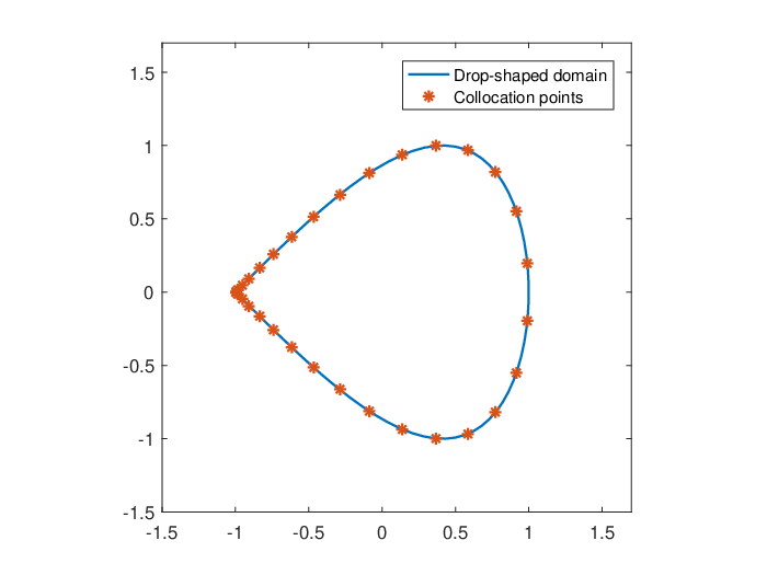
Refer to caption
(a) p=2,n=16p=2,n=16
Refer to caption
(b) p=2,n=16p=2,n=16
Figure 3. Collocation points on the drop-shaped and heart-shaped obstacles.
Table 4. Numerical errors for the drop-shaped domain with ω=π\omega=\pi.
Point source Plane wave
nn ‖ϕ∗−ϕ(n)‖L2\|\phi_{*}-\phi^{(n)}\|_{L^{2}} ‖ψ∗−ψ(n)‖L2\|\psi_{*}-\psi^{(n)}\|_{L^{2}} ‖ϕ(n∗)−ϕ(n)‖L2\|\phi^{(n_{*})}-\phi^{(n)}\|_{L^{2}} ‖ψ(n∗)−ψ(n)‖L2\|\psi^{(n_{*})}-\psi^{(n)}\|_{L^{2}}
16 2.0999e-03 2.1650e-03 4.5396e-01 5.8469e-01
32 2.4347e-08 3.1562e-08 3.9571e-03 4.9919e-03
64 1.2669e-08 1.6911e-08 2.7795e-04 3.7244e-04
128 3.8572e-10 5.1477e-10 2.4339e-05 2.8050e-05
256 1.1736e-11 1.5791e-11 1.1917e-04 1.6019e-04
512 1.3430e-14 1.7613e-14 9.2866e-06 1.2593e-05
1024 6.2155e-15 4.9608e-15 5.5606e-06 7.5428e-06
2048 6.1235e-15 5.9362e-15 1.1380e-07 1.5203e-07
Table 5. Numerical errors for the heart-shaped domain with ω=π\omega=\pi.
Point source Plane wave
nn ‖ϕ∗−ϕ(n)‖L2\|\phi_{*}-\phi^{(n)}\|_{L^{2}} ‖ψ∗−ψ(n)‖L2\|\psi_{*}-\psi^{(n)}\|_{L^{2}} ‖ϕ(n∗)−ϕ(n)‖L2\|\phi^{(n_{*})}-\phi^{(n)}\|_{L^{2}} ‖ψ(n∗)−ψ(n)‖L2\|\psi^{(n_{*})}-\psi^{(n)}\|_{L^{2}}
16 4.3673e-02 1.0523e-01 6.0929e-03 1.1896e-02
32 6.0075e-04 1.5144e-03 2.5014e-05 3.7337e-05
64 4.3721e-07 8.4011e-07 1.2432e-07 1.2820e-07
128 1.8692e-09 1.2039e-09 2.2355e-09 1.4398e-09
256 1.1752e-11 7.5236e-12 1.3571e-11 8.6880e-12
512 1.6306e-13 1.0433e-13 1.8443e-13 1.1843e-13
1024 4.5946e-15 4.0851e-15 8.0003e-15 5.9002e-15
2048 1.1742e-14 1.3828e-14 9.6079e-15 1.0804e-14

5.2. Numerical examples: nonsmooth obstacles

In this subsection, we assume that DD has a single corner at x0x_{0} and assume ΓD∖{x0}\Gamma_{D}\setminus\{x_{0}\} to be analytic. The angle γ\gamma at the corner is supposed to satisfy 0<γ<2​π0<\gamma<2\pi. Suppose that the corner point x0x_{0} corresponds to the parameter t=0t=0 in the parametric representation of ΓD\Gamma_{D}. To test the accuracy of our method, we adopt the exact solutions in form of (5.5) with the point source located at x¯=(0.1,0.2)⊤\bar{x}=(0.1,0.2)^{\top} and x¯=(−0.5,0.2)⊤\bar{x}=(-0.5,0.2)^{\top} for the drop-shaped and heart-shaped obstacles, respectively. The interior angles are γ=π/2\gamma=\pi/2 and γ=3​π/2\gamma=3\pi/2 for the drop-shaped and heart-shaped obstacles, respectively. The parameterizations of these two boundary curves are also shown in Table 1. In addition, we consider the case that the obstacle is illuminated by a compressional plane wave 𝒖inc\boldsymbol{u}^{\rm inc} which is given by

𝒖inc​(x)=d​ei​κ𝔭​d⋅x,\boldsymbol{u}^{\rm inc}(x)=d\mathrm{e}^{{\rm i}\kappa_{\mathfrak{p}}d\cdot x},

where d=(cos⁡θ,sin⁡θ)⊤d=(\cos\theta,\sin\theta)^{\top} is the unit propagation direction vector.

To resolve the field near the corner, we adopt the graded mesh by taking the substitution [7, 15] t=w⁡(s)t=w(s), which is given by

w⁡(s)=2​π​[v⁡(s)]p[v⁡(s)]p+[v⁡(2​π−s)]p,0≤s≤2​π,\displaystyle w(s)=2\pi\frac{[v(s)]^{p}}{[v(s)]^{p}+[v(2\pi-s)]^{p}},\qquad 0\leq s\leq 2\pi,

where

v⁡(s)=(1p−12)​(π−sπ)3+1p​s−ππ+12,p≥2,\displaystyle v(s)=\Big(\frac{1}{p}-\frac{1}{2}\Big)\Big(\frac{\pi-s}{\pi}\Big)^{3}+\frac{1}{p}\frac{s-\pi}{\pi}+\frac{1}{2},\qquad p\geq 2,

and is applied to the parametric curve of the drop-shaped and heart-shaped obstacles. In experiments, we choose sj:=π​j/n+π/(2​n)s_{j}:=\pi j/n+\pi/(2n) as the collocation points in (5.4). The generated points w⁡(sj)w(s_{j}), j=0,⋯,2​n−1j=0,\cdots,2n-1 of the graded mesh on the both boundaries are presented in Figure 3 for p=2p=2.

The numerical errors between the numerical solution and the exact solution (5.5) with L2​(∂B)L^{2}(\partial B) norm for the drop-shaped and heart-shaped obstacles are listed in Tables 4 and 5 with the angular frequency ω=π\omega=\pi and n~=16\tilde{n}=16. Additionally, we calculate the values of compressional and shear scattered fields ϕ(n∗),ψ(n∗)\phi^{(n_{*})},\psi^{(n_{*})} on ∂B\partial B with n~=16,n∗=4096\tilde{n}=16,n_{*}=4096 by the incident plane wave with θ=π/6\theta=\pi/6, and compare them with the cases of other numbers of collocation points. For the point source case, the solver quickly converges to machine precision for both domains. This is due to the analyticity of the artificial solution. On the other hand, for the true scattering problem, i.e., the scattering problem of the plane wave incidence, we note that the numerical error of the heart-shaped domain is better than that of the drop-shaped domain. The reason is apparently related to the concavity of the domain. Detailed analysis will be investigated in the future work.

6. Conclusion

We have proposed a novel boundary integral formulation and developed a highly accurate numerical method for solving the time-harmonic elastic scattering from a rigid bounded obstacle immersed in a homogeneous and isotropic elastic medium. Using the Helmholtz decomposition, we reduce the scattering problem to a coupled boundary integral equation with singular integral operators. By introducing an appropriate reqularizer to the coupled system, we split the operator equation in the form of an isomorphic operator plus a compact one. The convergence is shown for both the semi-discrete and full-discrete schemes via the trigonometric collocation method. Numerical experiments for smooth and nonsmooth obstacles, especially for the obstacles with corners, are presented to demonstrate the superior performance of the proposed method. Along this line, we intend to extend the current work to the coupled fluid-solid scattering problem and the three-dimensional elastic obstacle scattering problem, where the more complicated model equations need to be considered.

References

  • [1] J. F. Ahner and G. C. Hsiao, On the two-dimensional exterior boundary-value problems of elasticity, SIAM J. Appl. Math., 31 (1976), 677–685.
  • [2] B. Alpert, Hybrid Gauss-trapezoidal quadrature rules, SIAM J. Sci. Comput., 20 (1999) 1551–1584.
  • [3] H. Ammari, E. Bretin, J. Garnier, H. Kang, H. Lee, and A. Wahab, Mathematical Methods in Elasticity Imaging, Princeton University Press, New Jersey, 2015.
  • [4] A. Anand, J. Ovall, and C. Turc, Well conditioned boundary integral equations for two-dimensional sound-hard scattering problems in domains with corners, J. Integral Equ. Appl., 24 (2012), 1–38.
  • [5] G. Bao, L. Xu, and T. Yin, An accurate boundary element method for the exterior elastic scattering problem in two dimensions, J. Comput. Phys., 348 (2017), 343–363.
  • [6] F. Bu, J. Lin, and F. Reitich, A fast and high-order method for the three-dimensional elastic wave scattering problem, J. Comput. Phys., 258 (2014), 856–870.
  • [7] D. Colton and R. Kress, Inverse Acoustic and Electromagnetic Scattering Theory, 3rd edition, Springer, New York, 2013.
  • [8] H. Dong, J. Lai, and P. Li, Inverse obstacle scattering for elastic waves with phased or phaseless far-field data, SIAM J. Imaging Sci., 12 (2019), 809–838.
  • [9] H. Dong, J. Lai, and P. Li, An inverse acoustic-elastic interaction problem with phased or phaseless far-field data, Inverse Probl., 36 (2020), 035014.
  • [10] D. Givoli and J. B. Keller, Non-reflecting boundary conditions for elastic waves, Wave Motion, 12 (1990), 261–279.
  • [11] L. Greengard and S. Jiang, A new mixed potential representation for the equations of unsteady, incompressible flow, SIAM Review, 61 (2019), 733–755.
  • [12] G. Hu, A. Kirsch, and M. Sini, Some inverse problems arising from elastic scattering by rigid obstacles, Inverse Problems, 29 (2013), 015009
  • [13] A. Kirsch, An Introduction to the Mathematical Theory of Inverse Problems, 2nd edition, Springer, New York, 2011.
  • [14] A. Kirsch and S. Ritter, The Nyström method for solving a class of singular integral equations and applications in 3D-plate elasticity, Math. Meth. Appl. Sci., 22 (1999), 177–197.
  • [15] R. Kress, A Nyström method for boundary integral equations in domains with corners, Numer. Math., 58 (1990), 145–161.
  • [16] R. Kress, On the numerical solution of a hypersingular integral equation in scattering theory, J. Comput. Appl. Math., 61 (1995), 345–360.
  • [17] R. Kress, A collocation method for a hypersingular boundary integral equation via trigonometric differentiation, J. Integral Equ. Appl., 26 (2014), 197–213.
  • [18] R. Kress, Linear Integral Equations, 3rd edition, Springer, New York, 2014.
  • [19] R. Kress and I. H. Sloan, On the numerical solution of a logarithmic integral equation of the first kind for the Helmholtz equation, Numer. Math., 66 (1993), 199–214.
  • [20] J. Lai and P. Li, A framework for simulation of multiple elastic scattering in two dimensions, SIAM J. Sci. Comput., 41 (2019), A3276–A3299.
  • [21] L. D. Landau and E. M. Lifshitz, Theory of Elasticity, Oxford: Pergamon 1986.
  • [22] F. Le Louër, On the Fréchet derivative in elastic obstacle scattering, SIAM J. Appl. Math., 72 (2012), 1493–1507.
  • [23] F. Le Louër, A high order spectral algorithm for elastic obstacle scattering in three dimensions, J. Comput. Phys., 279 (2014), 1–17.
  • [24] S. G. Mikhlin and S. Prössdorf, Singular Integral Operators, Springer Verlag, Berlin, 1986.
  • [25] Y. H. Pao and V. Varatharajulu, Huygens’ principle, radiation conditions, and integral formulas for the scattering of elastic waves, J. Acoust. Soc. Amer., 59 (1976), 1361–1371.
  • [26] J. Saranen and G. Vainikko, Trigonometric collocation methods with product integration for boundary integral equations on closed curves, SIAM J. Numer. Anal., 33 (1996), 1577–1596.
  • [27] M. S. Tong and W. C. Chew, Nyström method for elastic wave scattering by three-dimensional obstacles, J. Comput. Phys., 226 (2007), 1845–1858.
  • [28] J. Yue, M. Li, P. Li, and X. Yuan, Numerical solution of an inverse obstacle scattering problem for elastic waves via the Helmholtz decomposition, Commun. Comput. Phys., 26 (2019), 809–837.