Effective Theory of Freeze-in Dark Matter

Cosmology based experiments like WMAP Hinshaw et al. 2013 and PLANCK Aghanim et al. 2018, through precise measurements of cosmic microwave background (CMB) anisotropies have suggested the presence of a mysterious, non-luminous and non-baryonic component of matter, known as dark matter (DM), giving rise to around $26\%$ of the present universe’s energy density. In terms of density parameter $\Omega_{\rm DM}$ and $h=\text{Hubble Parameter}/(100\;\text{km}~\text{s}^{-1}\text{Mpc}^{-1})$, the present DM abundance is conventionally reported as Aghanim et al. 2018: $\Omega_{\text{DM}}h^{2}=0.120\pm 0.001$ at 68% CL. While cosmology based evidences are relatively more recent, astrophysical evidences for DM emerged long back starting with the galaxy cluster observations by Fritz Zwicky Zwicky 1933 back in 1933, observations of galaxy rotation curves in 1970’s Rubin and Ford 1970 to the more recent observation of the bullet cluster Clowe et al. 2006. While all these evidences are purely based on gravitational interactions of DM, we do not have any knowledge about the particle aspects of DM. Since none of the Standard Model (SM) particles can satisfy the criteria for being a realistic DM candidate, several beyond standard model (BSM) proposals have been put forward out of which the weakly interacting massive particle (WIMP) Jungman et al. 1996; Bertone et al. 2005; Feng 2010; Arcadi et al. 2018 is the most popular one. WIMP paradigm considers thermal production of DM in the early universe from the SM bath Srednicki et al. 1988; Gondolo and Gelmini 1991 with an interesting coincidence that a DM particle having mass and couplings around the electroweak scale can give rise to the correct DM abundance after thermal freeze-out. This is often referred to as the WIMP Miracle Kolb and Turner 1990. The same interactions between DM and SM particles which lead to thermal production of DM, can also lead to DM-nucleon scattering with the possibility of leaving some signatures at direct detection experiments like LUX Akerib et al. 2017, PandaX-II Tan et al. 2016; Cui et al. 2017, XENON1T Aprile et al. 2017; Aprile et al. 2018. However, the continuous absence of such signal in several direct detection experiments so far have already constrained DM-nucleon scattering rates very strictly, pushing it towards the region where coherent neutrino-nucleus scattering cross section may dominate, also dubbed as the neutrino floor Billard et al. 2014. Similar null results for WIMP type DM have also been reported at indirect DM detection experiments, and also the large hadron collider (LHC), all of which constrain the coupling strength of DM with SM particles.

While negative results in WIMP searches do not necessarily rule it out, it has motivated the particle physics community to look for beyond the thermal WIMP paradigm where the interaction scale of DM particle can be much lower than the scale of weak interaction i.e.  DM may be more feebly interacting than the thermal WIMP paradigm. One such possibility is to consider the origin of DM to be purely non-thermal Hall et al. 2010. In such a scenario, DM interaction with the SM bath is so weak that it never attains thermal equilibrium at any epoch in the early universe. While the initial abundance of DM in such a scenario is negligible, it can be produced from out of equilibrium decays of heavy particles or annihilation of particles already present in the thermal plasma. Such a scenario where DM abundance freezes in from a negligible initial abundance to the observed abundance is known as freeze-in, and the candidates of such non-thermal DM produced via freeze-in are often classified into a group called FIMP (Feebly interacting) massive particle)(for a review on such a DM paradigm see, for example Bernal et al. 2017). If there exists renormalizable interactions between FIMP and the SM bath, then the non-thermal production of DM is effective at lowest possible temperature. If the mother particle is in thermal equilibrium with the bath then the maximum production of DM occurs when the temperature of the bath $T\simeq M_{0}$, the mass of mother particle. Therefore, the non-thermal criterion enforces the couplings to be extremely tiny via the following condition $\left|\dfrac{\Gamma}{{\bf H}}\right|_{T\simeq M_{0}}<1$ Arcadi and Covi 2013, where $\Gamma$ is the decay width. For the case of scattering, one has to replace $\Gamma$ by the interaction rate $n_{\rm eq}\,\langle\sigma{\rm v}\rangle$, $n_{eq}$ being the equilibrium number density of mother particle. These types of freeze-in scenarios are known as infra-red (IR)-freeze-in Yaguna 2011; Chu et al. 2012; Blennow et al. 2014; Merle and Totzauer 2015; Shakya 2016; Hessler et al. 2017; Biswas and Gupta 2016; König et al. 2016; Biswas and Gupta 2017; Biswas et al. 2017; Bernal et al. 2017; Biswas et al. 2018; Heeba et al. 2018; Peyman Zakeri et al. 2018; Becker 2019; Heeba and Kahlhoefer 2020; Lebedev and Toma 2019; Barman et al. 2020; Bhattacharya et al. 2020a; Koren and McGehee 2020 where DM production is dominated by the lowest possible temperature at which it can occur i.e. $T\sim M_{0}$, since for $T<M_{0}$, the number density of mother particle becomes Boltzmann suppressed. On the other hand, there exists another possibility where FIMP and SM sector are coupled via higher dimensional operators (dimension $d>4$) only. In such a scenario, DM production is effective at high temperatures and very much sensitive to initial history like the reheat temperature of the universe. Due to the higher dimensional nature of such interactions, DM production happens via scattering only, specially at a temperature above the electroweak scale. This particular scenario is known as the ultra-violet (UV) freeze-in Hall et al. 2010; Elahi et al. 2015; McDonald 2016; Chen and Kang 2018; Biswas et al. 2019; Bernal et al. 2019; Bernal et al. 2020a; Bernal et al. 2020b. It may also happen that a realistic FIMP scenario has a mixture of both IR as well as UV freeze-in where after a phase transition like the one at the electroweak scale, the DM can have renormalizable interactions with the SM bath. However, if DM mass is much higher than the scale of such phase transitions, then its production will be dominated by UV freeze-in only.

Motivated by these, in this work, we consider an effective field theory (EFT) approach for UV freeze-in of DM. Since scalar DM can have renormalizable interactions with the SM particles which no symmetries can prevent, we consider a singlet Majorana fermion, odd under a $Z_{2}$ stabilising symmetry, to be the DM candidate. Naturally, DM interactions with the SM particles can arise only at dimension (dim.) five or higher level, suppressed by appropriate powers of the cut-off scale. We first list out possible DM-SM operators upto dim.8. While calculating the DM relic abundance, we consider only scalar operators responsible for DM-SM interactions for simplicity. We then constrain the cut-off scale, DM mass, as well as reheat temperature from correct DM relic requirement by considering both UV as well as IR freeze-in contribution that may arise before and after electroweak symmetry breaking (EWSB) respectively. We find that the IR freeze-in contribution is sizeable only for dim.5 operators while it is negligible for higher dimensional operators unless we consider a very low reheat temperature $(\leq 1\;\text{TeV})$ of the universe. Also, as expected, such IR freeze-in contribution is insignificant if DM mass is above the electroweak scale. We then discuss the possibility of the same cut-off scale to be responsible or origin of light neutrino masses via Weinberg operators of dim.5 and 7 Weinberg 1979. We also briefly comment on the scenario where DM-SM interactions can happen only via lepton number violating operators. We then discuss some possible UV completion of a few DM-SM operators. Finally, we briefly comment upon the possibility of inflaton decay into DM at radiative level by virtue of the effective DM-SM operators and show the differences in parameter space compared to the ones obtained by considering DM production purely from SM-DM operators.

This paper is organised as follows. In section II we list out possible DM-SM operators upto and including dim. 8 followed by the details of possible interaction vertices that can arise before and after EWSB in section III. In section IV, we compute DM relic abundance by considering only DM scalar operators as mentioned before. In section V we consider the possibility of DM production only through dim. 5 and dim. 7 operators and check the constraints from neutrino mass if it is assumed to be arising from Weinberg operators of the same dimensions. In section VI we briefly comment upon different possibilities of generating DM-SM effective operators within a UV complete framework and in section VII we show the production of DM via one loop decay of the inflaton. We also show the effects of non-instantaneous reheating on DM abundance in section VIII and finally we conclude in section IX.

In this section we list out possible operators upto dim.8 that can be formed by considering bilinears in DM fields. EFT analysis in the context of the WIMP type DM has been done extensively and can be found in Beltran et al. 2009; Cao et al. 2011; Goodman et al. 2010; Cheung et al. 2012; De Simone et al. 2013; Matsumoto et al. 2014; Duch et al. 2015; Liem et al. 2016; Brod et al. 2018; Arina et al. 2020 and the references therein. Here we perform a similar study for the FIMP DM, considering it to be a singlet Majorana fermion $(\chi)$.

Since we are imposing a $Z_{2}$ symmetry for ensuring the stability of the DM, hence any interaction term involving the DM fields has to be at least bilinear in $\chi$. Due to the fact that the Majorana fermion is its own anti-particle, those bilinears which are odd under charge conjugation vanish identically. We first chalk out the bilinears that can be formed out of the DM fields with Majorana nature in Table 1. As we see, it is only possible to construct those operators which have scalar, axial vector and pseudoscalar interactions in the DM fields, while the vector current and dipole moments vanish. Since we are interested in UV freeze-in that requires the new physics at a scale $\Lambda\geq\rm TeV$, hence we can choose our EFT basis at the scale of $\Lambda$, and write all the operators below $\Lambda$. The generalised DM-SM non-renormalizable interaction in such case can be written as:

$\displaystyle\mathcal{L}\supset\frac{c_{ij}\mathcal{O}^{(d)j}_{\rm SM}\mathcal{O}^{(d^{{}^{\prime}})i}_{\rm DM}}{\Lambda_{ij}^{d+d^{{}^{\prime}}-4}},$

(1)

where $\mathcal{O}^{(d^{{}^{\prime}})}_{\rm DM}$ is a dark sector operator of mass dimension $d^{{}^{\prime}}$, $\mathcal{O}^{(d)}_{SM}$ is the operator in the visible sector of mass dimension $d$. The parameter $\Lambda_{ij}$ is a dimensionfull scale and $c_{ij}$ is the dimensionless Wilson coefficient. If $d+d^{{}^{\prime}}>4$, then the interaction is associated with an effective non-renormalizable operator of the form presented in Eq. (1). Since a DM bilinear itself makes up dim. 3, hence we need to construct gauge invariant Lorentz contracted SM operators upto dim.5. Now, there are 13 dimension 4, 1 dimension 5, 63 dimension 6 and 20 dimension 7 operators invariant under the Standard Model gauge group Lehman 2014. Four of the dimension 6 operators violate baryon number conservation, leaving 59 that conserve baryon number Lehman 2014; Grzadkowski et al. 2010. As mentioned earlier, we consider SM operators upto dim.5 only which take part in DM-SM interactions, which amounts to a maximum dimension of eight for DM-SM operators. This not only limits the number of operators but also ensures the kinematics involved in scattering processes to be simple. All DM-SM interactions are encoded by higher-dimensional operators, with a cut-off scale $\Lambda$, which is the mass scale of the heavy fields integrated out to obtain the low-energy Lagrangian:

$\displaystyle\mathcal{L}=\mathcal{L}_{\text{SM}}+\mathcal{L}_{\text{DM}}+\mathcal{L}_{5}+\mathcal{L}_{7}+\mathcal{L}_{8},$

(2)

where $\mathcal{L}_{\text{SM(DM)}}$ is the renormalizable SM (DM) Lagrangian and $\mathcal{L}_{d}$ corresponds to the operators of dimension $d>4$.

In the renormalizable level the Lagrangian for the DM field has the form:

$\displaystyle\mathcal{L}_{\text{DM}}=i\overline{\chi^{c}}\not{\partial}\chi-M_{\chi}\overline{\chi^{c}}\chi,$

(3)

as the DM is electroweak singlet with zero hypercharge. In Table 2 we list the possible operators that can be built out of SM and DM fields upto dimension 8. Generically, the EFT description is valid as long as $\Lambda\gtrsim\frac{M_{\chi}}{2\pi}$ Busoni et al. 2014; Busoni et al. 2015 and hence it is justified to integrate out the heavy fields with masses roughly of the order of the cut-off scale. But in case of UV freeze-in scenario, as we shall see, the reheat temperature of the universe is also involved which we consider to be $\gtrsim\text{TeV}$. Hence in our prescription the EFT framework is valid as long as $\Lambda\gtrsim\frac{M_{\chi}}{2\pi},T_{\text{RH}}$. The formulation of the EFT at scale $\mu$ depends on which degrees of freedom are relevant at that particular scale. The operators we have listed in Table 2 are in the basis of unbroken electroweak phase, valid at or above the electroweak scale $\mu=\mu_{\text{EW}}\sim m_{Z}$.

In this section we would like to specify all the decay and annihilation processes that can lead to the freeze-in production of the DM. As mentioned earlier, before EWSB, DM interacts with SM bath only via $n\to m$ scattering processes (with $n,m\geq 2$) arising out of higher dimensional operators (UV freeze-in) whereas in the post-EWSB phase there exists the possibility of IR freeze-in as well via decays. Therefore, we discuss DM interactions during pre- and post-EWSB phases separately in the following subsections.

In this section we would like to compute the freeze-in yield of the DM $\chi$ before and after EWSB. Since the dark sector and visible sector in our case communicate via operators of different dimension suppressed by powers of some high scale $\Lambda$ as shown in Eq. (1), it leads to the UV freeze-in scenario before EWSB. In this case the yield is completely determined by the cut-off scale $\Lambda$ and the reheat temperature $T_{\text{RH}}$ of the universe¹¹ 1 Once inflation ends, the thermalisation of the universe occurs, leading to a radiation dominated phase. This is the reheating epoch Allahverdi et al. 2010, which takes the universe to a radiation-dominated phase after the end of inflation. Success of the big bang nucleosynthesis (BBN) puts a lower bound on the reheating temperature i.e. $T_{\text{RH}}\gtrsim\mathcal{O}(1)$ MeV de Salas et al. 2015.. Before EWSB, all SM fields have zero mass, but the DM is still massive because of its bare mass, while after EWSB all the SM particles acquire masses. Since one can then expand the scalar field around its minima, the decay channels also appear along with the $n\to 2$ annihilation processes. Also, before EWSB, as we have seen in the last section, there are no decay channels that lead to DM production. In order to determine the DM abundance at present temperature, we need to solve the Boltzmann equation (BEQ) to obtain the number density of $\chi$. The BEQs involved in this case are elaborated in Appendix. B.2,  B.3 and B.4.

The decay processes after EWSB are dominantly $1\to 2$, where the Higgs decays to produce a pair of DM particles, if kinematically allowed. As one can understand, since the decay happens in the rest frame of the mother particle, hence the mass of the decaying particle is involved in this case (i.e., the Higgs mass). As a consequence, decay always gives rise to IR freeze-in, where the yield does not depend on the reheat temperature, in contrast to standard UV freeze-in set-up. Also, since only Higgs decay is involved in our case, hence the DM mass $M_{\chi}$ is necessarily below $m_{h}/2\sim 62~\rm GeV$ in order to have non-zero contribution from decay. After EWSB there is also one gluon initiated process that can produce DM in the final state via Higgs mediation through a triangle loop (as shown in Fig. 2). The effective $ggH$ coupling has the form: $\frac{-ig_{s}^{2}}{32\pi^{2}}\frac{m_{h}^{2}}{v_{h}}\mathcal{F}\left(x\right)$ Buschmann et al. 2015, where $\mathcal{F}\left(x\right)=x\biggl[1+\left(1-x\right)f\left(x\right)\biggr]$ with

$$f(x)=\left\{\begin{array}[]{ll}\Bigg(\sin^{-1}\sqrt{\frac{1}{x}}\Bigg)^{2},~~x>1\\ -\frac{1}{4}\Bigg({\text{ln}}\Biggl[\frac{1+\sqrt{1-x}}{1-\sqrt{1-x}}\Biggr]-i\pi\Bigg)^{2}~~x<1,\\ \end{array}\right.$$

and $x=\frac{4m_{t}^{2}}{m_{h}^{2}}$, where we are considering only top quark contribution in the triangle loop. Total yield due to annihilation and decay after EWSB is therefore coming from both IR and UV processes.

Before going into the details of the Boltzmann equation (BEQ) for determining the DM relic abundance, we would first like to put a constraint on the cut-off scale $\Lambda$ such that the DM is out of equilibrium, ensuring its non-thermal production. In order to determine that, we need to calculate the scattering rate and compare it with the corresponding Hubble rate, the details of which can be found in Appendix. E. In Fig. 3 we have shown the constraint on $\Lambda$ in the bi-dimensional plane of $T-\Lambda$ such that the DM-SM interaction is always out of equilibrium. In the plot, the straight line contours with different colours correspond to the condition $\mathcal{R}=\frac{\Gamma_{n\to 2}}{H}=1$ for dimension 5 (red), 7 (green) and 8 (blue) operators. Here $H(T)=\sqrt{\frac{\pi^{2}}{90}g_{\star\rho}(T)}T^{2}/M_{pl}$ is the Hubble rate with $g_{\star\rho}(T)$ being the relativistic energy degrees of freedom at temperature T, and $M_{pl}$ is the Planck mass. The region to the left of each contour is where the DM thermalises with the SM bath. As the rate goes roughly as $\mathcal{R}\propto\frac{TM_{pl}}{\Lambda^{n}}$, hence the condition for thermalisation: $T.M_{pl}\gtrsim\Lambda^{n}$, also overlaps with the condition where the effective formalism breaks down: $T>\Lambda^{n}$. For operators with higher dimension the DM can be kept out of equilibrium for a smaller $\Lambda$ as $\mathcal{R}\sim\frac{1}{\Lambda^{n}}$, while lower dimensional operators need a larger $\Lambda$ to ensure non-thermal DM production. This is exactly reflected in Fig. 3, where we see for dim.8 interaction $\Lambda\gtrsim 10^{4}~\rm GeV$ is the minimum cut-off scale that guarantees that the DM remains out of thermal equilibrium, while dim.5 demands $\Lambda\gtrsim 10^{10}~\rm GeV$.

The Boltzmann equation (BEQ) for the DM yield consists of all the processes that appear before and after EWSB, which includes decay and scattering diagrams. The yield is defined as the ratio of DM number density $n_{\chi}$ to the entropy density $s$: $Y_{\chi}=n_{\chi}/s$, where $s=\frac{2\pi^{2}}{45}g_{\star s}(T)T^{3}$ and $g_{\star s}$ is the relativistic entropy of degrees of freedom. BEQ corresponding to decay is derived in Appendix. B.1, while those due to the scatterings are elaborated in Appendix. B.2,  B.3 and B.4. Now, the total yield at present epoch (at temperature $T_{0}$) is a sum of the contribution from yield before EWSB and yield after EWSB, which can be written as:

$\displaystyle\begin{split}Y_{\chi}^{\text{total}}\left(T_{0}\right)_{T_{\text{RH}}>T_{\text{EW}}}&\simeq\Biggl[\Bigg\{\int_{T_{\text{EW}}}^{T_{\text{RH}}}dT\frac{1}{512\pi^{6}}\int_{T_{\text{EW}}}^{T_{\text{RH}}}\frac{dT}{s(T).H(T)}\int_{0}^{\infty}dsd\Omega\left(\frac{\sqrt{s}}{2}\right)^{2}\overline{\left|\mathcal{M}\right|}^{2}_{12\to 34}\\ &\frac{1}{\sqrt{s}}K_{1}\left(\frac{\sqrt{s}}{T}\right)\Bigg\}+\Bigg\{\int_{T_{\text{EW}}}^{T_{\text{RH}}}\frac{dT}{s(T).H(T)}\frac{1}{64\left(2\pi\right)^{7}}\\ &\int_{0}^{\infty}dss^{3/2}\overline{\left|\mathcal{M}\right|}^{2}_{123\to 45}K_{1}\left(\frac{\sqrt{s}}{T}\right)\int_{0}^{1}dx_{1}\int_{1-x_{1}}^{1}dx_{2}\Bigg\}+\\ &\Bigg\{\int_{T_{\text{EW}}}^{T_{\text{RH}}}\frac{dT}{s(T).H(T)}\frac{1}{64\left(2\pi\right)^{9}}\int_{0}^{\infty}ds\sqrt{s}\overline{\left|\mathcal{M}\right|}^{2}_{1234\to 56}K_{1}\left(\frac{\sqrt{s}}{T}\right)\\ &\int_{0}^{\sqrt{s}}ds_{12}\int_{0}^{(\sqrt{s}-\sqrt{s_{12}})^{2}}ds_{34}\sqrt{1+\frac{s_{12}^{2}}{s^{2}}-\frac{2s_{12}s_{34}}{s^{2}}+\frac{s_{34}^{2}}{s^{2}}-\frac{2s_{12}}{s}-\frac{2s_{34}}{s}}\\ &\int\frac{d\cos\theta_{12}}{2}\int\frac{d\cos\theta_{34}}{2}\Bigg\}\Biggr]+\Biggl[\int_{T_{\text{0}}}^{T_{\text{EW}}}dT\frac{m_{h}^{2}\Gamma_{h\to\chi\chi}}{2\pi^{2}}\frac{K_{1}\left(m_{h}/T\right)}{s(T).H(T)}+\\ &\frac{1}{512\pi^{6}}\int_{T_{\text{0}}}^{T_{\text{EW}}}\frac{dT}{s(T).H(T)}\int_{\text{max}\left(4M_{\chi}^{2},4m_{\text{SM}}^{2}\right)}^{\infty}dsd\Omega\frac{1}{4}\sqrt{\left(s-4m_{\text{SM}}^{2}\right)\left(s-4M_{\chi}^{2}\right)}\\ &\overline{\left|\mathcal{M}\right|}^{2}_{12\to 34}\frac{1}{\sqrt{s}}K_{1}\left(\frac{\sqrt{s}}{T}\right)\Biggr]\end{split}$

(18)

where the first big parenthesis $\biggl[...\biggr]$ takes care of the yield before EWSB that includes contributions from $n\to m$ processes. The second big parenthesis $\biggl[...\biggr]$ includes contribution from processes after EWSB due to $1\to 2$ decay and $2\to 2$ annihilations. Also note that in case of yield after EWSB the lower limit of the integration depends on the mass of the particles involved in the process. One can then obtain the relic abundance of the DM at present epoch using:

$\displaystyle\Omega_{\chi}h^{2}=2.75\times 10^{8}\frac{M_{\chi}}{\text{GeV}}Y^{\text{total}}_{\chi}\left(T_{0}\right),$

(19)

which need to satisfy the PLANCK Aghanim et al. 2018 observed limit: $\Omega_{\text{DM}}h^{2}=0.120\pm 0.001$.

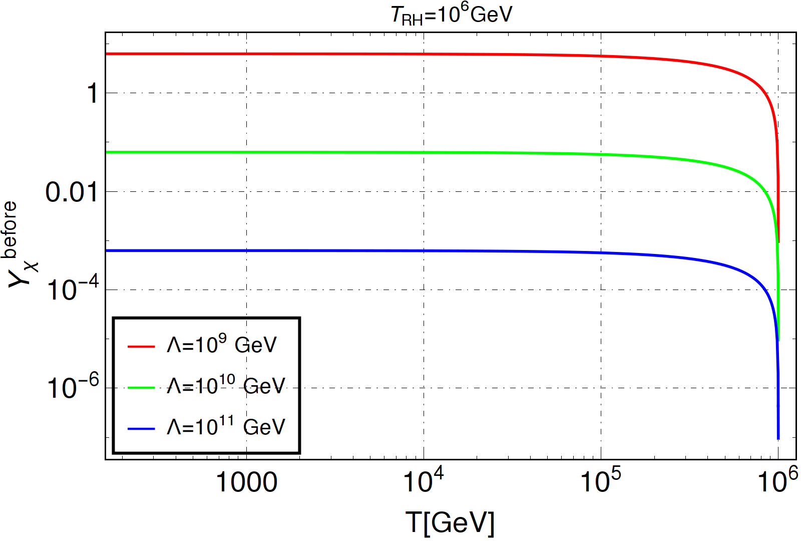
The contributions of operators with different dimensions to the DM yield (before and after EWSB) are shown in Fig. 4, where in both the plots the red, green and blue curves correspond to dim.5, dim.7 and dim.8 operators respectively. Although the final yield, as evident from Eq. (18), is a sum of the yield before and after EWSB, this exercise helps us to understand the dynamics of the DM yield with the bath temperature before and after EW symmetry breaking occurs. This also indicates which processes dominate over the others. Here we see, dim.5 interactions always have dominant contribution over the others both before and after the EWSB. This leads us to the fact that dim.5 interactions play the deciding role in determining the total yield as well as the DM relic abundance. In Fig. 5 we have illustrated how the DM yield varies with the bath temperature before and after EWSB separately when all the operators with different dimensions are considered together. In the top left panel of Fig. 5 we have shown the variation of DM yield $Y_{\chi}$ with temperature $T$ considering all $n\to 2$ channels before EWSB for a fixed reheat temperature $T_{\text{RH}}=10^{6}~\rm GeV$ for illustration. With the change in the effective scale $\Lambda$ the yield also changes as shown by the red, green and blue curves corresponding to $\Lambda=\{10^{9},10^{10},10^{11}\}~\rm GeV$ respectively, and as expected, for larger $\Lambda$ the yield is small. As the reheat temperature is fixed, hence all the curves originate from the same point at high temperature and the yield becomes maximum at $T\sim T_{\text{RH}}$. The yield freezes-in immediately $T\sim T_{\text{RH}}$, which is a typical feature of UV freeze-in. Since we are considering the era before EWSB, all SM particles are massless, but the DM, because of its bare Majorana mass, is still massive. However, the yield is very loosely dependent on the DM mass because of the involvement of two large scales in the theory, namely the cut-off scale and the reheat temperature. As a result ignoring the DM mass does not change the outcome. In the top right panel of Fig. 5 we have again shown how the DM yield before EWSB varies with the temperature for a fixed choice of the effective scale $\Lambda=10^{10}~\rm GeV$. In this case we choose three different reheat temperature: $\{10^{6},10^{7},10^{8}\}~\rm GeV$ to illustrate the effects on $Y_{\chi}$. As we can notice, with the change in $T_{\text{RH}}$ the upper limit of the integration in the first parenthesis of Eq. (18) changes, resulting in the change in corresponding yield. For larger $T_{\text{RH}}$ we achieve a larger yield following Eq. (18). Also, all the curves originate from different $T$ with the change in $T_{\text{RH}}$, but the flavour of UV freeze-in prevails as the yield in each case is maximum at $T\sim T_{\text{RH}}$. Note that, all these curves end before the electroweak phase transition temperature $T_{EW}\simeq 160~\rm GeV$ ensuring DM production only before EWSB era and hence dominance of UV freeze-in. In the bottom left panel of Fig. 5 we illustrate contribution from different $n\to 2$ processes, where the red curve is due to $2\to 2$, the blue and green curves are for $3\to 2$ and $2\to 3$ and the black curve is due to $4\to 2$ processes. As expected, the $2\to 2$ processes dominate over all the others. Although the $2\to 3$ and $3\to 2$ processes almost overlap on each other, but a close scrutiny (see inset) shows that $2\to 3$ processes are more relevant than $3\to 2$, while $4\to 2$ processes are the most suppressed ones. The $3\to 3$ processes are also sub-dominant in the presence of $2\to 3$ and $3\to 2$ processes, hence we do not show them here. Finally, in the bottom right panel of Fig. 5 we have shown the yield after EWSB when all SM particles are considered to be massive along with the DM. We consider the IR dominated $1\to 2$ decay and all $2\to 2$ annihilation channels that lead to DM pair production. Since all the states are massive, the $2\to 2$ channels dominate over other $n\to 2$ channels for $n>2$. As a result, we only consider the decay and $2\to 2$ annihilation processes in this regime. Here we show the variation of yield for DM mass $M_{\chi}:\{5~\text{keV},50~\text{GeV}\}$. For both the cases the $h\to\chi\chi$ channel also contributes, while for $M_{\chi}>m_{h}/2$ only $2\to 2$ annihilation channels contribute. Due to the absence of decay modes the yield after EWSB is negligibly small for DM masses larger than the EWSB scale²² 2 For exmple, the yield after EWSB corresponding to a DM of mass 500 GeV is $\sim 10^{-13}$ at $T\simeq 0.1~\rm GeV$.. For a DM with mass $\sim\text{keV}$ the yield saturates at $T\sim 10~\text{GeV}$, much earlier than BBN. This implies that there is no damping in the matter power spectrum due to late DM formation, which otherwise puts a very strong bound on the DM mass Irˇsič et al. 2017; Murgia et al. 2018. Note that, in the presence of decay, the yield after EWSB is comparable with that before EWSB. Note here, due to the effect of IR freeze-in, the DM freezes in when $x=m/T\sim\mathcal{O}(1)$. Also note that these yields do not correspond to the right relic abundance, rather these are just to illustrate how the DM yield builds up with the temperature.

In Fig. 6 we have shown the parameter space satisfying PLANCK observed relic abundance in $\Lambda-T_{\text{RH}}$ plane for different choices of the DM mass. The relic abundance is computed using Eq. (19) with all the dimensions taken into account together. We choose DM masses $M_{\chi}:\{50~\text{MeV},50~\text{GeV},500~\text{GeV}\}$ (clockwise from top left) for illustrating the resulting parameter space. We also have shown that a DM mass of 3.55 keV satisfies the desired relic abundance in the bottom right panel of Fig. 6. DM with mass in that ballpark has received lots of attention in the context of the 3.55 keV $X$-ray observation Bulbul et al. 2014; Boyarsky et al. 2014; Boyarsky et al. 2015; Mambrini and Toma 2015; Cappelluti et al. 2018; Cappelluti et al. 2018. In the top left panel of Fig. 6 we show the region satisfying relic abundance for a DM mass of 50 MeV. Here all points satisfy the observed relic abundance. For DM mass $M_{\chi}<m_{h}/2$, the $h\to\chi\chi$ channel plays the important role as it enhances the DM yield after EWSB. Since after EWSB IR freeze-in dominates (as all the states are massive), hence we see a part of the parameter space independent of the reheat temperature. This corresponds to $\Lambda\sim 10^{13}~\rm GeV$ for $M_{\chi}=50~\rm MeV$ and $\Lambda\sim 10^{15}~\rm GeV$ for $M_{\chi}=50~\rm GeV$ (top right panel). Beyond $T_{\text{RH}}\sim 10^{7}~\rm GeV$, $\Lambda$ rises linearly with $T_{\text{RH}}$ for $M_{\chi}=50~\rm MeV$ as UV freeze-in starts contributing. For $M_{\chi}=50~\rm GeV$ this linear rise starts at $T_{\text{RH}}\sim 10^{6}~\rm GeV$ (top right panel). We have also shown the percentage contribution to the observed relic abundance coming from processes before and after EWSB in the top panel plots and also in the bottom right panel. Here we see more than 60% contribution to observed relic abundance from processes before EWSB comes at a larger reheat temperature (red points). This means UV freeze-in is more effective for larger $T_{\text{RH}}$. This is understandable as from Eq. (18) we see that $Y_{\chi}^{\text{UV}}\propto T_{\text{RH}}$ as we are considering $T_{\text{EW}}<<T_{\text{RH}}$. Now, a larger $T_{\text{RH}}$ also calls for a larger $\Lambda$ to satisfy the relic abundance as from Eq. (19) we see that for a fixed DM mass $\Omega_{\chi}\propto\frac{T_{\text{RH}}}{\Lambda^{n}}$. Contribution from processes after EWSB is more profound at a lower reheat temperature where IR freeze-in dominates (blue points). As explained before, in that region the relic abundance is almost independent of the reheat temperature, which is again attributed to Eq. (18), where we see $Y_{\chi}^{\text{IR}}\propto T_{\text{EW}}$ as $T_{0}<<T_{\text{EW}}$. For DM mass $\leq T_{\text{EW}}$ this pattern remains the same as evident from the top panel and bottom right panel plots. On the other hand, for DM mass of 500 GeV (left bottom panel of Fig. 6) all of the contribution comes from processes before EWSB (as $M_{\chi}>T_{\text{EW}}$) where only UV freeze-in is in action. As a result, there is a linear rise of $\Lambda$ with the increase in reheat temperature throughout. Note that, in this case, the reheat temperature can also be $\sim\text{TeV}$ as for a massive DM one has to dial down the reheat temperature in order to satisfy the relic abundance since $\Omega_{\chi}\propto\frac{M_{\chi}T_{\text{RH}}}{\Lambda^{n}}$. This is also reflected in the other plots where we see for a lighter DM one requires a larger $T_{\text{RH}}$ to obtain the right abundance. One important point to note here is the fact that in presence of all the operators, dim.5 interactions dominate over the others which is understandable from the $\frac{1}{\Lambda}$ suppression compared to other dimensions where the suppression is even stronger.

In Fig. 6 we have considered possible operators upto dim.8 where naturally dim.5 operators dominate. We have taken all operators at the same time to analyse the parameter space allowed by relic abundance. The required cut-off scale in the vertical axes of the plots shown in Fig. 6 clearly depicts the dominance of dim.5 operator. However, depending on the UV completion, only one such dimension may be allowed for DM-SM operators. For a comparison, we show the corresponding scanned plots for a scenario where DM-SM interaction occurs only through dim.8 scalar operators in Fig. 7. While the correlation of the reheat temperature and the cut-off scale remains the same as in Fig. 6, but the required $\Lambda$ becomes substantially small as one can expect. Another interesting observation is that, as we go to higher dimensional operators for DM-SM interactions beyond dim.5, the IR freeze-in contribution to DM relic becomes more and more negligible, specially when reheat temperature of the universe is kept well above 1 TeV.

Within the SM field content it is possible to generate light neutrino Majorana mass via operators of different mass dimension that violate lepton number by two units $(\Delta L=2)$ Babu and Leung 2001; de Gouvea and Jenkins 2008; Angel et al. 2013; Cepedello et al. 2017; Gargalionis et al. 2020; Herrero-García and Schmidt 2019 and are suppressed by some scale $\Lambda_{\nu}$. Thus, a more natural explanation for the smallness of $m_{\nu}$ is that they are generated (via some underlying new physics) at a scale $\Lambda_{\nu}$ (higher than the electroweak scale), and manifest themselves at low energies through effective higher dimensional operators. As we know, $d=5$ seesaw operators are the lowest dimensional effective neutrino mass operators. Now, for such a dim.5 operator one can express the light neutrino mass in terms of the Higgs VEV and the effective scale $\Lambda_{\nu}$ at which the lepton number is broken:

$\displaystyle m_{\nu}\simeq\frac{v_{h}^{2}}{\Lambda_{\nu}},$

(20)

which indicates that in order to generate light neutrino mass in the right ballpark the scale $\Lambda_{\nu}\gtrsim 10^{11}~\rm TeV$. Similarly, for neutrino mass generated from lepton number violating SM operators in dim.7, one can write:

$\displaystyle m_{\nu}\simeq\frac{v_{h}^{4}}{\Lambda_{\nu}^{3}},$

(21)

which gives rise to $\Lambda_{\nu}\gtrsim 10^{3}~\rm TeV$ in order to get neutrino mass in the desired ballpark. Now, a non-zero neutrino mass can be generated only after EWSB, while DM relic abundance has contribution both from processes before after EWSB. In order to make a connection between the freeze-in scale and the scale at which light neutrino mass can be generated, we compare the freeze-in scale considering only dim.5 and dim.7 interactions where it is also possible to generate neutrino mass via SM operators.

In Fig. 8 we show regions satisfying the PLANCK observed relic abundance in $T_{\text{RH}}-\Lambda$ bi-dimensional plane for a fixed DM mass of 50 GeV. In the left panel we depict the parameter space for only dim.5 DM-SM operator and in the right panel we show the same where the contribution comes only from dim.7 DM-SM interactions. While the relative contribution of UV and IR freeze-in contribution for dim.5 operator will be similar to the ones shown in Fig. 6, for dim.7 the effect of IR freeze-in is negligible as noted before for dim.8 operator. This is because for dim.7, due to the cut-off scale suppression, in order to make the post-EWSB processes effective, the reheat temperature has to go below $\sim 1~\text{TeV}$. We are not considering reheat temperature below a TeV as mentioned earlier. In both the plots we also show minimum $\Lambda_{\nu}$ required to get light neutrino mass (Eq. (20), Eq. (21)) via the black dashed lines. Hence, in both cases all of the region above the black dashed line is compatible with the neutrino mass. From both the plots it is evident that $\Lambda$ required for right relic abundance both in the case of dim.5 and dim.7 coincide with $\Lambda_{\nu}$ obtained from Eq. (20) and Eq. (21). This indicates, the scale of UV freeze-in where only dim.5 and dim.7 operators contribute, can simultaneously explain light neutrino mass. Such a possibility of simultaneous origin of neutrino mass and DM-SM operator through effective operators that violate lepton number, in turn, constrains the reheat temperature of the universe as seen from the plots.

Several possibilities have been discussed in the literature which naturally give rise to feeble DM-SM couplings. For example, the authors of Biswas et al. 2018 considered loop suppressions as origin of FIMP interactions, in Mambrini et al. 2013; Bhattacharyya et al. 2018 the possibility of DM-SM interactions via superheavy neutral gauge bosons was discussed. On the other hand, the authors of Kim and McDonald 2017; Kim and McDonald 2018 considered clockwork origin of FIMP couplings. In this section, we briefly comment upon the possibility of generating some of the DM-SM effective operators within a complete theory. This is similar to the UV completion of the Weinberg operator of light neutrino masses Weinberg 1979 via seesaw mechanism Minkowski 1977; Gell-Mann et al. 1979; Mohapatra and Senjanovic 1980; Schechter and Valle 1980; Mohapatra and Senjanovic 1981; Lazarides et al. 1981; Wetterich 1981; Schechter and Valle 1982.

Let us start with the dim.5 operator between DM and SM. The only possible scalar operator is $(\overline{\chi^{c}}\chi)(H^{\dagger}H)/\Lambda$. If we consider a UV complete theory, where in addition to the $Z_{2}$ odd DM, there exists a pair of vector like lepton doublet $\psi_{L,R}$ odd under the same $Z_{2}$ symmetry, the additional relevant terms in the Lagrangian are

$$-\mathcal{L}\supset M_{\psi}\overline{\psi}\psi+Y_{1}\overline{\psi_{L}}\tilde{H}\chi+Y_{2}\overline{\psi^{c}_{R}}H\chi+{\rm h.c.}$$

(22)

At a scale $\mu\ll M_{\psi}$, the heavy vector like leptons can be integrated out, resulting in an operator like $(\overline{\chi^{c}}\chi)(H^{\dagger}H)Y_{1}Y_{2}/M_{\psi}$. If reheat temperature of the universe is smaller than $M_{\psi}$, these additional vector like leptons are not present in the thermal bath and hence DM-SM interactions mimic as a dimension five operator with a cut-off $\Lambda=M_{\psi}$.

Similarly, one can generate dimension seven operator of the type $(\overline{\chi^{c}}\chi)(H^{\dagger}H)^{2}/\Lambda^{3}$. Consider the presence of $Z_{2}$ odd singlet fermion $\psi_{L}$ and a $Z_{2}$ even singlet scalar $\phi$. The relevant new terms in the Lagrangian are

$$-\mathcal{L}\supset M_{\psi}\overline{\psi^{c}_{L}}\psi_{L}+\left(Y_{1}\overline{\psi_{L}}\phi\chi+{\rm h.c.}\right)+\mu_{\phi}\phi H^{\dagger}H+M^{2}_{\phi}\phi\phi$$

(23)

At a scale $\mu\ll M_{\psi},M_{\phi},\mu_{\phi}$, the heavy fields $\psi_{L},\phi$ can be integrated out, resulting in DM-SM operator of the type $(\overline{\chi^{c}}\chi)(H^{\dagger}H)^{2}Y^{2}_{1}\mu^{2}_{\phi}/(M^{4}_{\phi}M_{\psi})$. Considering $\mu_{\phi}\approx M_{\psi}\approx M_{\phi}\approx\Lambda$ and order one Yukawa couplings, this leads to the expected dimension seven operator $(\overline{\chi^{c}}\chi)(H^{\dagger}H)^{2}/\Lambda^{3}$. In the same way, one can also generate other operators discussed in the above analysis.

In this section we look into the possibility of DM production from the decay of inflaton. Since we are interested in freeze-in production of DM via effective DM-SM operators, we do not consider any direct coupling of inflaton to DM. However, inflaton has direct couplings to the SM particles, required for reheating Allahverdi et al. 2010. In such a scenario, even though inflaton does not have direct coupling with DM at tree level, one can not ignore the decay of the inflaton to the DM via SM loops Kaneta et al. 2019. As we extensively have shown earlier the dominance of dim.5 operator over the others for DM production via freeze-in, hence we only show the results for such dim.5 interaction where the DM is produced via one-loop decay of the inflaton as shown in Fig. 9. We neglect direct coupling of the DM to the inflaton and consider the following effective Lagrangian between the inflaton, SM Higgs, SM fermions and the DM $\chi$:

$\displaystyle\mathcal{L}\supset\mu_{h}\phi_{I}\left(H^{\dagger}H\right)+y_{f}\phi_{I}ff+\frac{1}{\Lambda}\overline{\chi^{c}}\chi\left(H^{\dagger}H\right),$

(24)

where $\mu_{h}$ is the Higgs-inflaton coupling (having mass dimension one) which we consider to be as large as the inflaton mass, and $y_{f}$ is the SM fermion-inflaton Yukawa coupling, which is considered to be of order one. The one-loop decay of the inflaton via Higgs exchange is given by:

$\displaystyle\Gamma_{\phi_{I}}^{\text{loop}}=\frac{M_{I}}{2\pi}L^{2},$

(25)

with the loop contribution

$\displaystyle L=\frac{\mu_{h}}{16\pi^{2}\Lambda}\Biggl(1+\ln\Bigl[\frac{\Lambda^{2}}{M_{I}^{2}}\Bigr]\Biggr)$

(26)

the details of which can be found in Appendix F. Here we have ignored the masses of the SM particles as well as that of the DM since the inflaton itself is very heavy and the decay happens at a very high temperature. Now, the tree-level inflaton decay to the Higgs and to the SM fermions is given by:

$\displaystyle\begin{split}\Gamma_{\phi_{I}\to hh}&=\frac{\mu_{h}^{2}}{16\pi M_{I}};~~\Gamma_{\phi_{I}\to ff}&=\frac{N_{c}y_{f}^{2}}{8\pi}M_{I}.\end{split}$

(27)

We define the branching ratio of inflaton decay into DM at one-loop as

$\displaystyle\begin{split}{\rm Br}&=\frac{\Gamma_{\phi_{I}}^{\text{loop}}}{\Gamma_{\phi_{I}\to hh}+\Gamma_{\phi_{I}\to ff}+\Gamma_{\phi_{I}}^{\text{loop}}}.\end{split}$

(28)

Following the prescriptions in Chung et al. 1999; Giudice et al. 2001; Garcia et al. 2017; Kaneta et al. 2019 for non-instantaneous thermalization (finite decay width of the inflaton) one can write the relic abundance of the DM due to inflaton decay as:

$\displaystyle\begin{split}\Omega_{\chi}^{\text{inf}}h^{2}&=M_{\chi}{\rm Br}\Biggl(\frac{T_{\text{RH}}}{M_{I}}\Biggr).\end{split}$

(29)

where the reheat temperature is defined via:

$\displaystyle\frac{3}{2}cH\left(T_{\text{RH}}\right)=\Gamma_{\phi_{I}},$

(30)

$c$ being a numerical constant taken to be $c\approx 1.2$ Pradler and Steffen 2007; Ellis et al. 2016; Kaneta et al. 2019 and $H\left(T_{\text{RH}}\right)$ is the Hubble parameter at $T=T_{\rm RH}$. Next, we compute the bound on the reheat temperature, branching fraction and cut-off scale with the condition that the inflaton decay gives rise to all of the observed DM density. We consider only inflaton decay as the source of DM production, for large cut-off scales which we consider, production from thermal bath is negligible at this stage as was shown by the authors of Kaneta et al. 2019.

In the left panel of Fig. 10 we show the parameter space for PLANCK observed relic density for inflaton mass of $M_{I}=10^{12}~\rm GeV$. For each value of $\{\Lambda,{\rm Br}\}$ the DM mass $M_{\chi}$ needed to obtain the correct relic abundance is colour coded by the scale at the right of the plot. Note that, for lighter DM mass one naturally requires a larger branching ratio, as expected from Eq. (29). The black dashed line in this figure corresponds to the branching ratio following Eq. (28), applicable to the particular dim.5 DM-SM effective operator we consider here. In other regions of this plot, the branching ratio is independently varied so that correct DM relic is obtained for chosen DM mass and cutoff scale. In the right panel of Fig. 10 we show the PLANCK allowed parameter space in $T_{\text{RH}}-\Lambda$ plane where for each value of $\{\Lambda,T_{\text{RH}}\}$ the required $M_{\chi}$ to obtain right relic abundance is shown by the colour code. Since the reheat temperature has an inverse relation with the branching ratio according to Eq. (30), hence in this plot we see a complementary dependence of DM mass for different $T_{\text{RH}}$ on the cut-off scale. It is interesting to note that, correct DM abundance for such dim.5 scenario can be produced from radiative inflaton decay for a relatively smaller value of cut-off scale $\Lambda$ compared to what we found in our previous analysis considering only DM-SM operators to be responsible for DM production. This can be realised by comparing the parameter space shown in Fig. 10 with the ones in Fig. 6 and 8.

In calculating the DM relic abundance in Sec. IV we made a crucial assumption: $Y_{\chi}\left(T=T_{\text{RH}}\right)=0$, which implies that the DM abundance is zero at the end of reheating when the the thermal bath reaches an equilibrium temperature $T=T_{\text{RH}}$. Such an assumption is very commonplace in freeze-in analysis which takes into account the fact that the reheat temperature is the largest temperature that the thermal bath can achieve, which is true if reheating is an instantaneous process. The reheat temperature $(T_{\text{RH}})$ is usually calculated by assuming an instantaneous conversion of the energy density in the inflaton field into radiation when the decay width of the inflaton is equal to the Hubble expansion rate. In reality, however, reheating is not an instantaneous process Chung et al. 1999; Giudice et al. 2001; Kaneta et al. 2019. For example, if the inflaton is described by a simple model with quadratic potential, the radiation dominated phase follows a prolonged stage of matter domination during which the energy density of the universe is dominated by the coherent oscillations of the inflaton field. For different choices of inflaton potential, the equation of state during this pre-reheating or preheating phase can be different from the one in matter dominated phase. The temperature of the thermal bath during this phase can reach a value much larger than $T_{\text{RH}}$ and is typically denoted by: $T_{\text{max}}\sim\left(H_{I}M_{\text{pl}}\right)^{1/4}\sqrt{T_{\text{RH}}}$, where for a simple model of inflation $H_{I}$ can be identical with the inflaton mass Chung et al. 1999. The temperature subsequently comes down from $T_{\text{max}}$ to $T_{\text{RH}}$ when the inflaton decay is completed. The DM, thus can be produced at a temperature $T=T_{\text{max}}$ (i.e., prior to the inflation ends), which is higher than $T_{\text{RH}}$. This practically indicates that the DM can have a non-zero abundance at $T=T_{\text{RH}}$ when the inflaton decay is completed and the radiation dominated era begins.

We consider that the inflaton decays dominantly into the radiation, and the DM is not produced in thermal equilibrium during reheating. With this assumption, to determine the DM abundance at $T=T_{\text{RH}}$, one has to first solve a set of coupled BEQ involving the inflaton density $\rho_{\phi}$ and the radiation density $\rho_{R}$ Kaneta et al. 2019 in order to find the evolution of temperature with expansion of the universe:

$\displaystyle\begin{split}&\dot{\rho_{\phi}}+3H\rho_{\phi}=-\Gamma_{\phi}\rho_{\phi}\\ &\dot{\rho_{R}}+4H\rho_{R}=\Gamma_{\phi}\rho_{\phi}\\ &H^{2}=\frac{\rho_{\phi}}{3M_{\text{pl}}^{2}}+\frac{\rho_{R}}{3M_{\text{pl}}^{2}},\end{split}$

(31)

$\displaystyle R_{\text{ann}}=\frac{T^{\xi+6}}{\Lambda^{\xi+2}}.$

(32)

with the BEQ for the DM number density evolution being:

$\displaystyle\dot{n_{\chi}}+3Hn_{\chi}=R_{\text{ann}}.$

(33)

Note that, the annihilation rate in Eq. (32) corresponds to a cross section Bernal et al. 2020b:

$\displaystyle\langle\sigma v\rangle=\frac{T^{\xi}}{\Lambda^{\xi+2}},$

(34)

$\displaystyle n_{\chi}\left(T_{\text{RH}}\right)\simeq\left\{\begin{array}[]{ll}\frac{24\sqrt{30}}{5g{{}_{\star\rho}}(T)\pi}\frac{T_{\text{RH}}^{\xi+4}M_{\text{pl}}}{\left(6-\xi\right)\Lambda^{\xi+2}},~~\xi<6\\ \frac{24\sqrt{30}}{5g{{}_{\star\rho}}(T)\pi}\frac{M_{\text{pl}}T_{\text{RH}}^{10}}{\Lambda^{8}}\log\Bigl(\frac{T_{\text{max}}}{T_{\text{RH}}}\Bigr)~~,\xi=6\\ \frac{24\sqrt{30}}{5g{{}_{\star\rho}}(T)\pi}\frac{T_{\text{max}}^{\xi-6}T_{\text{RH}}^{10}}{\left(\xi-6\right)\Lambda^{\xi+2}}~~,\xi>6.\end{array}\right.$

The DM relic abundance at present epoch for a mass $M_{\chi}$ can be deduced from Eq. (VIII):

$\displaystyle\Omega_{\chi}h^{2}\simeq 6\times 10^{6}\Biggl[\frac{n\left(T_{\text{RH}}\right)}{T^{3}_{\text{RH}}}\Biggr]\Biggl(\frac{M_{\chi}}{\text{GeV}}\Biggr).$

(39)

References

- Hinshaw et al. (2013) G. Hinshaw et al. (WMAP), Astrophys. J. Suppl. 208, 19 (2013), arXiv:1212.5226 [astro-ph.CO] .
- Aghanim et al. (2018) N. Aghanim et al. (Planck), (2018), arXiv:1807.06209 [astro-ph.CO] .
- Zwicky (1933) F. Zwicky, Helv. Phys. Acta 6, 110 (1933), [Gen. Rel. Grav.41,207(2009)].
- Rubin and Ford (1970) V. C. Rubin and W. K. Ford, Jr., Astrophys. J. 159, 379 (1970).
- Clowe et al. (2006) D. Clowe, M. Bradac, A. H. Gonzalez, M. Markevitch, S. W. Randall, C. Jones, and D. Zaritsky, Astrophys. J. 648, L109 (2006), arXiv:astro-ph/0608407 [astro-ph] .
- Jungman et al. (1996) G. Jungman, M. Kamionkowski, and K. Griest, Phys. Rept. 267, 195 (1996), arXiv:hep-ph/9506380 [hep-ph] .
- Bertone et al. (2005) G. Bertone, D. Hooper, and J. Silk, Phys. Rept. 405, 279 (2005), arXiv:hep-ph/0404175 [hep-ph] .
- Feng (2010) J. L. Feng, Ann. Rev. Astron. Astrophys. 48, 495 (2010), arXiv:1003.0904 [astro-ph.CO] .
- Arcadi et al. (2018) G. Arcadi, M. Dutra, P. Ghosh, M. Lindner, Y. Mambrini, M. Pierre, S. Profumo, and F. S. Queiroz, Eur. Phys. J. C78, 203 (2018), arXiv:1703.07364 [hep-ph] .
- Srednicki et al. (1988) M. Srednicki, R. Watkins, and K. A. Olive, Nucl. Phys. B310, 693 (1988), [,247(1988)].
- Gondolo and Gelmini (1991) P. Gondolo and G. Gelmini, Nucl. Phys. B360, 145 (1991).
- Kolb and Turner (1990) E. W. Kolb and M. S. Turner, Front. Phys. 69, 1 (1990).
- Akerib et al. (2017) D. S. Akerib et al. (LUX), Phys. Rev. Lett. 118, 021303 (2017), arXiv:1608.07648 [astro-ph.CO] .
- Tan et al. (2016) A. Tan et al. (PandaX-II), Phys. Rev. Lett. 117, 121303 (2016), arXiv:1607.07400 [hep-ex] .
- Cui et al. (2017) X. Cui et al. (PandaX-II), (2017), arXiv:1708.06917 [astro-ph.CO] .
- Aprile et al. (2017) E. Aprile et al. (XENON), Phys. Rev. Lett. 119, 181301 (2017), arXiv:1705.06655 [astro-ph.CO] .
- Aprile et al. (2018) E. Aprile et al., (2018), arXiv:1805.12562 [astro-ph.CO] .
- Billard et al. (2014) J. Billard, L. Strigari, and E. Figueroa-Feliciano, Phys. Rev. D89, 023524 (2014), arXiv:1307.5458 [hep-ph] .
- Hall et al. (2010) L. J. Hall, K. Jedamzik, J. March-Russell, and S. M. West, JHEP 03, 080 (2010), arXiv:0911.1120 [hep-ph] .
- Bernal et al. (2017) N. Bernal, M. Heikinheimo, T. Tenkanen, K. Tuominen, and V. Vaskonen, Int. J. Mod. Phys. A32, 1730023 (2017), arXiv:1706.07442 [hep-ph] .
- Arcadi and Covi (2013) G. Arcadi and L. Covi, JCAP 1308, 005 (2013), arXiv:1305.6587 [hep-ph] .
- Yaguna (2011) C. E. Yaguna, JHEP 08, 060 (2011), arXiv:1105.1654 [hep-ph] .
- Chu et al. (2012) X. Chu, T. Hambye, and M. H. G. Tytgat, JCAP 1205, 034 (2012), arXiv:1112.0493 [hep-ph] .
- Blennow et al. (2014) M. Blennow, E. Fernandez-Martinez, and B. Zaldivar, JCAP 1401, 003 (2014), arXiv:1309.7348 [hep-ph] .
- Merle and Totzauer (2015) A. Merle and M. Totzauer, JCAP 1506, 011 (2015), arXiv:1502.01011 [hep-ph] .
- Shakya (2016) B. Shakya, Mod. Phys. Lett. A31, 1630005 (2016), arXiv:1512.02751 [hep-ph] .
- Hessler et al. (2017) A. G. Hessler, A. Ibarra, E. Molinaro, and S. Vogl, JHEP 01, 100 (2017), arXiv:1611.09540 [hep-ph] .
- Biswas and Gupta (2016) A. Biswas and A. Gupta, JCAP 1609, 044 (2016), [Addendum: JCAP1705,no.05,A01(2017)], arXiv:1607.01469 [hep-ph] .
- König et al. (2016) J. König, A. Merle, and M. Totzauer, JCAP 1611, 038 (2016), arXiv:1609.01289 [hep-ph] .
- Biswas and Gupta (2017) A. Biswas and A. Gupta, JCAP 1703, 033 (2017), [Addendum: JCAP1705,no.05,A02(2017)], arXiv:1612.02793 [hep-ph] .
- Biswas et al. (2017) A. Biswas, S. Choubey, and S. Khan, JHEP 02, 123 (2017), arXiv:1612.03067 [hep-ph] .
- Biswas et al. (2018) A. Biswas, D. Borah, and A. Dasgupta, (2018), arXiv:1805.06903 [hep-ph] .
- Heeba et al. (2018) S. Heeba, F. Kahlhoefer, and P. Stöcker, JCAP 1811, 048 (2018), arXiv:1809.04849 [hep-ph] .
- Peyman Zakeri et al. (2018) S. Peyman Zakeri, S. Mohammad Moosavi Nejad, M. Zakeri, and S. Yaser Ayazi, Chin. Phys. C42, 073101 (2018), arXiv:1801.09115 [hep-ph] .
- Becker (2019) M. Becker, Eur. Phys. J. C79, 611 (2019), arXiv:1806.08579 [hep-ph] .
- Heeba and Kahlhoefer (2020) S. Heeba and F. Kahlhoefer, Phys. Rev. D101, 035043 (2020), arXiv:1908.09834 [hep-ph] .
- Lebedev and Toma (2019) O. Lebedev and T. Toma, Phys. Lett. B798, 134961 (2019), arXiv:1908.05491 [hep-ph] .
- Barman et al. (2020) B. Barman, S. Bhattacharya, and M. Zakeri, JCAP 02, 029 (2020), arXiv:1905.07236 [hep-ph] .
- Bhattacharya et al. (2020a) S. Bhattacharya, N. Chakrabarty, R. Roshan, and A. Sil, JCAP 04, 013 (2020a), arXiv:1910.00612 [hep-ph] .
- Koren and McGehee (2020) S. Koren and R. McGehee, Phys. Rev. D 101, 055024 (2020), arXiv:1908.03559 [hep-ph] .
- Elahi et al. (2015) F. Elahi, C. Kolda, and J. Unwin, JHEP 03, 048 (2015), arXiv:1410.6157 [hep-ph] .
- McDonald (2016) J. McDonald, JCAP 1608, 035 (2016), arXiv:1512.06422 [hep-ph] .
- Chen and Kang (2018) S.-L. Chen and Z. Kang, JCAP 05, 036 (2018), arXiv:1711.02556 [hep-ph] .
- Biswas et al. (2019) A. Biswas, S. Ganguly, and S. Roy, (2019), 10.1088/1475-7516/2020/03/043, arXiv:1907.07973 [hep-ph] .
- Bernal et al. (2019) N. Bernal, F. Elahi, C. Maldonado, and J. Unwin, JCAP 11, 026 (2019), arXiv:1909.07992 [hep-ph] .
- Bernal et al. (2020a) N. Bernal, J. Rubio, and H. Veermäe, JCAP 06, 047 (2020a), arXiv:2004.13706 [hep-ph] .
- Bernal et al. (2020b) N. Bernal, J. Rubio, and H. Veermäe, (2020b), arXiv:2006.02442 [hep-ph] .
- Weinberg (1979) S. Weinberg, Phys. Rev. Lett. 43, 1566 (1979).
- Beltran et al. (2009) M. Beltran, D. Hooper, E. W. Kolb, and Z. C. Krusberg, Phys. Rev. D 80, 043509 (2009), arXiv:0808.3384 [hep-ph] .
- Cao et al. (2011) Q.-H. Cao, C.-R. Chen, C. S. Li, and H. Zhang, JHEP 08, 018 (2011), arXiv:0912.4511 [hep-ph] .
- Goodman et al. (2010) J. Goodman, M. Ibe, A. Rajaraman, W. Shepherd, T. M. Tait, and H.-B. Yu, Phys. Rev. D 82, 116010 (2010), arXiv:1008.1783 [hep-ph] .
- Cheung et al. (2012) K. Cheung, P.-Y. Tseng, Y.-L. S. Tsai, and T.-C. Yuan, JCAP 05, 001 (2012), arXiv:1201.3402 [hep-ph] .
- De Simone et al. (2013) A. De Simone, A. Monin, A. Thamm, and A. Urbano, JCAP 02, 039 (2013), arXiv:1301.1486 [hep-ph] .
- Matsumoto et al. (2014) S. Matsumoto, S. Mukhopadhyay, and Y.-L. S. Tsai, JHEP 10, 155 (2014), arXiv:1407.1859 [hep-ph] .
- Duch et al. (2015) M. Duch, B. Grzadkowski, and J. Wudka, JHEP 05, 116 (2015), arXiv:1412.0520 [hep-ph] .
- Liem et al. (2016) S. Liem, G. Bertone, F. Calore, R. Ruiz de Austri, T. M. Tait, R. Trotta, and C. Weniger, JHEP 09, 077 (2016), arXiv:1603.05994 [hep-ph] .
- Brod et al. (2018) J. Brod, A. Gootjes-Dreesbach, M. Tammaro, and J. Zupan, JHEP 10, 065 (2018), arXiv:1710.10218 [hep-ph] .
- Arina et al. (2020) C. Arina, A. Cheek, K. Mimasu, and L. Pagani, (2020), arXiv:2005.12789 [hep-ph] .
- Lehman (2014) L. Lehman, Phys. Rev. D 90, 125023 (2014), arXiv:1410.4193 [hep-ph] .
- Grzadkowski et al. (2010) B. Grzadkowski, M. Iskrzynski, M. Misiak, and J. Rosiek, JHEP 10, 085 (2010), arXiv:1008.4884 [hep-ph] .
- Busoni et al. (2014) G. Busoni, A. De Simone, E. Morgante, and A. Riotto, Phys. Lett. B 728, 412 (2014), arXiv:1307.2253 [hep-ph] .
- Busoni et al. (2015) G. Busoni, A. De Simone, T. Jacques, E. Morgante, and A. Riotto, JCAP 03, 022 (2015), arXiv:1410.7409 [hep-ph] .
- Allahverdi et al. (2010) R. Allahverdi, R. Brandenberger, F.-Y. Cyr-Racine, and A. Mazumdar, Ann. Rev. Nucl. Part. Sci. 60, 27 (2010), arXiv:1001.2600 [hep-th] .
- de Salas et al. (2015) P. F. de Salas, M. Lattanzi, G. Mangano, G. Miele, S. Pastor, and O. Pisanti, Phys. Rev. D92, 123534 (2015), arXiv:1511.00672 [astro-ph.CO] .
- Buschmann et al. (2015) M. Buschmann, D. Goncalves, S. Kuttimalai, M. Schonherr, F. Krauss, and T. Plehn, JHEP 02, 038 (2015), arXiv:1410.5806 [hep-ph] .
- Irˇsič et al. (2017) V. Irˇsič et al., Phys. Rev. D 96, 023522 (2017), arXiv:1702.01764 [astro-ph.CO] .
- Murgia et al. (2018) R. Murgia, V. Irˇsič, and M. Viel, Phys. Rev. D 98, 083540 (2018), arXiv:1806.08371 [astro-ph.CO] .
- Bulbul et al. (2014) E. Bulbul, M. Markevitch, A. Foster, R. K. Smith, M. Loewenstein, and S. W. Randall, Astrophys. J. 789, 13 (2014), arXiv:1402.2301 [astro-ph.CO] .
- Boyarsky et al. (2014) A. Boyarsky, O. Ruchayskiy, D. Iakubovskyi, and J. Franse, Phys. Rev. Lett. 113, 251301 (2014), arXiv:1402.4119 [astro-ph.CO] .
- Boyarsky et al. (2015) A. Boyarsky, J. Franse, D. Iakubovskyi, and O. Ruchayskiy, Phys. Rev. Lett. 115, 161301 (2015), arXiv:1408.2503 [astro-ph.CO] .
- Mambrini and Toma (2015) Y. Mambrini and T. Toma, Eur. Phys. J. C 75, 570 (2015), arXiv:1506.02032 [hep-ph] .
- Cappelluti et al. (2018) N. Cappelluti, E. Bulbul, A. Foster, P. Natarajan, M. C. Urry, M. W. Bautz, F. Civano, E. Miller, and R. K. Smith, Astrophys. J. 854, 179 (2018), arXiv:1701.07932 [astro-ph.CO] .
- Babu and Leung (2001) K. Babu and C. N. Leung, Nucl. Phys. B 619, 667 (2001), arXiv:hep-ph/0106054 .
- de Gouvea and Jenkins (2008) A. de Gouvea and J. Jenkins, Phys. Rev. D 77, 013008 (2008), arXiv:0708.1344 [hep-ph] .
- Angel et al. (2013) P. W. Angel, N. L. Rodd, and R. R. Volkas, Phys. Rev. D 87, 073007 (2013), arXiv:1212.6111 [hep-ph] .
- Cepedello et al. (2017) R. Cepedello, M. Hirsch, and J. Helo, JHEP 07, 079 (2017), arXiv:1705.01489 [hep-ph] .
- Gargalionis et al. (2020) J. Gargalionis, I. Popa-Mateiu, and R. R. Volkas, JHEP 03, 150 (2020), arXiv:1912.12386 [hep-ph] .
- Herrero-García and Schmidt (2019) J. Herrero-García and M. A. Schmidt, Eur. Phys. J. C 79, 938 (2019), arXiv:1903.10552 [hep-ph] .
- Mambrini et al. (2013) Y. Mambrini, K. A. Olive, J. Quevillon, and B. Zaldivar, Phys. Rev. Lett. 110, 241306 (2013), arXiv:1302.4438 [hep-ph] .
- Bhattacharyya et al. (2018) G. Bhattacharyya, M. Dutra, Y. Mambrini, and M. Pierre, Phys. Rev. D 98, 035038 (2018), arXiv:1806.00016 [hep-ph] .
- Kim and McDonald (2017) J. Kim and J. McDonald, (2017), arXiv:1709.04105 [hep-ph] .
- Kim and McDonald (2018) J. Kim and J. McDonald, (2018), arXiv:1804.02661 [hep-ph] .
- Minkowski (1977) P. Minkowski, Phys. Lett. B67, 421 (1977).
- Gell-Mann et al. (1979) M. Gell-Mann, P. Ramond, and R. Slansky, Supergravity Workshop Stony Brook, New York, September 27-28, 1979, Conf. Proc. C790927, 315 (1979), arXiv:1306.4669 [hep-th] .
- Mohapatra and Senjanovic (1980) R. N. Mohapatra and G. Senjanovic, Phys. Rev. Lett. 44, 912 (1980).
- Schechter and Valle (1980) J. Schechter and J. W. F. Valle, Phys. Rev. D22, 2227 (1980).
- Mohapatra and Senjanovic (1981) R. N. Mohapatra and G. Senjanovic, Phys. Rev. D23, 165 (1981).
- Lazarides et al. (1981) G. Lazarides, Q. Shafi, and C. Wetterich, Nucl. Phys. B181, 287 (1981).
- Wetterich (1981) C. Wetterich, Nucl. Phys. B187, 343 (1981).
- Schechter and Valle (1982) J. Schechter and J. W. F. Valle, Phys. Rev. D25, 774 (1982).
- Kaneta et al. (2019) K. Kaneta, Y. Mambrini, and K. A. Olive, Phys. Rev. D 99, 063508 (2019), arXiv:1901.04449 [hep-ph] .
- Chung et al. (1999) D. J. H. Chung, E. W. Kolb, and A. Riotto, Phys. Rev. D60, 063504 (1999), arXiv:hep-ph/9809453 [hep-ph] .
- Giudice et al. (2001) G. F. Giudice, E. W. Kolb, and A. Riotto, Phys. Rev. D64, 023508 (2001), arXiv:hep-ph/0005123 [hep-ph] .
- Garcia et al. (2017) M. A. G. Garcia, Y. Mambrini, K. A. Olive, and M. Peloso, Phys. Rev. D 96, 103510 (2017), arXiv:1709.01549 [hep-ph] .
- Pradler and Steffen (2007) J. Pradler and F. D. Steffen, Phys. Lett. B 648, 224 (2007), arXiv:hep-ph/0612291 .
- Ellis et al. (2016) J. Ellis, M. A. G. Garcia, D. V. Nanopoulos, K. A. Olive, and M. Peloso, JCAP 03, 008 (2016), arXiv:1512.05701 [astro-ph.CO] .
- Banerjee et al. (2020) U. Banerjee, J. Chakrabortty, S. Prakash, and S. U. Rahaman, (2020), arXiv:2004.12830 [hep-ph] .
- Ahmed et al. (2018) A. Ahmed, M. Duch, B. Grzadkowski, and M. Iglicki, Eur. Phys. J. C78, 905 (2018), arXiv:1710.01853 [hep-ph] .
- Edsjo and Gondolo (1997) J. Edsjo and P. Gondolo, Phys. Rev. D 56, 1879 (1997), arXiv:hep-ph/9704361 .
- Tanabashi and Hagiwara (2018) M. Tanabashi and e. a. Hagiwara (Particle Data Group), Phys. Rev. D 98, 030001 (2018).
- Cline et al. (2017) J. M. Cline, H. Liu, T. Slatyer, and W. Xue, Phys. Rev. D 96, 083521 (2017), arXiv:1702.07716 [hep-ph] .
- Pierre (2018) M. Pierre, Dark Matter phenomenology : from simplified WIMP models to refined alternative solutions, Ph.D. thesis, Orsay (2018), arXiv:1901.05822 [hep-ph] .
- Bhattacharya et al. (2020b) S. Bhattacharya, P. Ghosh, and S. Verma, JCAP 01, 040 (2020b), arXiv:1904.07562 [hep-ph] .