跳到论文正文
W Papers独立论文阅读器 arXiv:2007.08703 论文正文 计算阅读时间 · 0%
引用这篇论文根据当前论文元数据生成,正式投稿前建议核对。


License: arXiv.org perpetual non-exclusive license
arXiv:2007.08703v1 [cs.LG] 17 Jul 2020

Bandits for BMO Functions

Tianyu Wang Correspondence to: tianyu@cs.duke.edu Affiliation: Department of Computer Science, Duke University, Durham, NC, USA    Cynthia Rudin Affiliation: Department of Computer Science, Duke University, Durham, NC, USA
Abstract

We study the bandit problem where the underlying expected reward is a Bounded Mean Oscillation (BMO) function. BMO functions are allowed to be discontinuous and unbounded, and are useful in modeling signals with infinities in the domain. We develop a toolset for BMO bandits, and provide an algorithm that can achieve poly-log δ\delta-regret – a regret measured against an arm that is optimal after removing a δ\delta-sized portion of the arm space.

Keywords: 
Machine Learning, ICML

1 Introduction

Multi-Armed Bandit (MAB) problems model sequential decision making under uncertainty. Algorithms for this problem have important real-world applications including medical trials (Robbins 1952) and web recommender systems (Li et al. 2010). While bandit methods have been developed for various settings, one problem setting that has not been studied, to the best of our knowledge, is when the expected reward function is a Bounded Mean Oscillation (BMO) function in a metric measure space. Intuitively, a BMO function does not deviate too much from its mean over any ball, and can be discontinuous or unbounded.

Such unbounded functions can model many real-world quantities. Consider the situation in which we are optimizing the parameters of a process (e.g., a physical or biological system) whose behavior can be simulated. The simulator is computationally expensive to run, which is why we could not exhaustively search the (continuous) parameter space for the optimal parameters. The “reward” of the system is sensitive to parameter values and can increase very quickly as the parameters change. In this case, by failing to model the infinities, even state-of-the-art continuum-armed bandit methods fail to compute valid confidence bounds, potentially leading to underexploration of the important part of the parameter space, and they may completely miss the optima.

As another example, when we try to determine failure modes of a system or simulation, we might try to locate singularities in the variance of its outputs. These are cases where the variance of outputs becomes extremely large. In this case, we can use a bandit algorithm for BMO functions to efficiently find where the system is most unstable.

There are several difficulties in handling BMO rewards. First and foremost, due to unboundedness in the expected reward functions, traditional regret metrics are doomed to fail. To handle this, we define a new performance measure, called δ\delta-regret. The δ\delta-regret measures regret against an arm that is optimal after removing a δ\delta-sized portion of the arm space. Under this performance measure, and because the reward is a BMO function, our attention is restricted to a subspace on which the expected reward is finite. Subsequently, strategies that conform to the δ\delta-regret are needed.

To develop a strategy that handles δ\delta-regret, we leverage the John-Nirenberg inequality, which plays a crucial role in harmonic analysis. We construct our arm index using the John-Nirenberg inequality, in addition to a traditional UCB index. In each round, we play an arm with highest index. As we play more and more arms, we focus our attention on regions that contain good arms. To do this, we discretize the arm space adaptively, and carefully control how the index evolves with the discretization. We provide two algorithms – Bandit-BMO-P and Bandit-BMO-Z. They discretize the arm space in different ways. In Bandit-BMO-P, we keep a strict partitioning of the arm space. In Bandit-BMO-Z, we keep a collection of cubes where a subset of cubes form a discretization. Bandit-BMO-Z achieves poly-log δ\delta-regret with high probability.

2 Related Works

Bandit problems in different settings have been actively studied since as far back as Thompson 1933. Upper confidence bound (UCB) algorithms remain popular (Robbins 1952; Lai and Robbins 1985; Auer 2002) among the many approaches for (stochastic) bandit problems (Srinivas et al. 2010; Abbasi-Yadkori et al. 2011; Agrawal and Goyal 2012; Bubeck and Slivkins 2012; Seldin and Slivkins 2014, e.g., see). Various extensions of upper confidence bound algorithms have been studied. Some works use KL-divergence to construct the confidence bound (Lai and Robbins 1985; Garivier and Cappé 2011; Maillard et al. 2011), and some works include variance estimates within the confidence bound (Audibert et al. 2009; Auer and Ortner 2010). UCB is also used in the contextual setting (Li et al. 2010; Krause and Ong 2011; Slivkins 2014, e.g.,).

Perhaps Lipschitz bandits are closest to BMO bandits. The Lipschitz bandit problem was termed “continuum-armed bandits” in early stages (Agrawal 1995). In “continuum-armed bandits,” arm space is continuous – e.g., [0,1][0,1]. Along this line, bandits that are Lipschitz continuous (or Hölder continuous) have been studied. In particular, Kleinberg 2005 proves a Ω⁡(T2/3)\Omega(T^{2/3}) lower bound and proposes a 𝒪~​(T2/3)\widetilde{\mathcal{O}}\left(T^{2/3}\right) algorithm. Under other extra conditions on top of Lipschitzness, regret rate of 𝒪~​(T1/2)\widetilde{\mathcal{O}}(T^{1/2}) was achieved (Cope 2009; Auer et al. 2007). For general (doubling) metric spaces, the Zooming bandit algorithm (Kleinberg et al. 2008) and Hierarchical Optimistic Optimization algorithm (Bubeck et al. 2011a) were developed. In more recent years, some attention has been given to Lipschitz bandit problems with certain extra conditions. To name a few, Bubeck et al. 2011b study Lipschitz bandits for differentiable rewards, which enables algorithms to run without explicitly knowing the Lipschitz constants. The idea of robust mean estimators (Bubeck et al. 2013; Bickel et al. 1965; Alon et al. 1999) was applied to the Lipschitz bandit problem to cope with heavy-tail rewards, leading to the development of a near-optimal algorithm (Lu et al. 2019). Lipschitz bandits with an unknown metric, where a clustering is used to infer the underlying unknown metric, has been studied by Wanigasekara and Yu 2019. Lipschitz bandits with discontinuous but bounded rewards were studied by Krishnamurthy et al. 2019.

An important setting that is beyond the scope of the aforementioned works is when the expected reward is allowed to be unbounded. This setting breaks the previous Lipschitzness assumption or “almost Lipschitzness” assumption (Krishnamurthy et al. 2019), which may allow discontinuities but require boundedness. To the best of our knowledge, this paper is the first work that studies the bandit learning problem for BMO functions.

3 Preliminaries

We review the concept of (rectangular) Bounded Mean Oscillation (BMO) in Euclidean space (Fefferman 1979; Stein and Murphy 1993, e.g.,).

Definition 1.

(BMO Functions) Let (ℝd,μ)(\mathbb{R}^{d},\mu) be the Euclidean space with the Lebesgue measure. Let Ll​o​c1​(ℝd,μ)L^{1}_{loc}(\mathbb{R}^{d},\mu) denote the space of measurable functions (on ℝd\mathbb{R}^{d}) that are locally integrable with respect to μ\mu. A function f∈Ll​o​c1​(ℝd,μ)f\in L^{1}_{loc}(\mathbb{R}^{d},\mu) is said to be a Bounded Mean Oscillation function, f∈B​M​O​(ℝd,μ)f\in BMO(\mathbb{R}^{d},\mu), if there exists a constant CfC_{f}, such that for any hyper-rectangles Q⊂ℝdQ\subset\mathbb{R}^{d},

1μ⁡(Q)​∫Q|f−⟨f⟩Q|​𝑑μ≤Cf,⟨f⟩Q:=∫Qf​𝑑μμ⁡(Q).\displaystyle\frac{1}{\mu(Q)}\int_{Q}|f-\left<f\right>_{Q}|d\mu\leq C_{f},\quad\left<f\right>_{Q}:=\frac{\int_{Q}fd\mu}{\mu(Q)}. (1)

For a given such function ff, the infimum of the admissible constant CfC_{f} over all hyper-rectangles QQ is denoted by ‖f‖B​M​O\|f\|_{BMO}, or simply ‖f‖\|f\|. We use ‖f‖B​M​O\|f\|_{BMO} and ‖f‖\|f\| interchangeably in this paper.

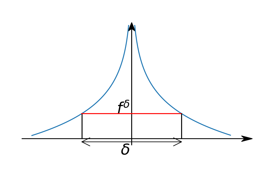
A BMO function can be discontinuous and unbounded. The function in Figure 1 illustrates the singularities a BMO function can have over its domain. Our problem is most interesting when multiple singularities of this kind occur.

To properly handle the singularities, we will need the John-Nirenberg inequality (Theorem 1), which plays a central role in our paper.

Theorem 1 (John-Nirenberg inequality).

Let μ\mu be the Lebesgue measure. Let f∈B​M​O​(ℝd,μ)f\in BMO\left(\mathbb{R}^{d},\mu\right). Then there exists constants C1C_{1} and C2C_{2}, such that, for any hypercube q⊂ℝdq\subset\mathbb{R}^{d} and any λ>0\lambda>0,

μ⁡({x∈q:|f⁡(x)−⟨f⟩q|>λ})≤C1​μ​(q)​exp⁡{−λC2​‖f‖}.\displaystyle\mu\hskip-2.0pt\left(\hskip-1.0pt\left\{\hskip-1.0ptx\hskip-1.0pt\in\hskip-1.0ptq:\hskip-1.0pt\left|f\hskip-1.0pt(x)\hskip-1.0pt-\hskip-1.0pt\left<f\right>_{q}\right|\hskip-1.0pt>\hskip-1.0pt\lambda\hskip-1.0pt\right\}\hskip-1.0pt\right)\hskip-1.0pt\leq\hskip-1.0ptC_{1}{\mu(q)}\exp\left\{\hskip-1.0pt\frac{-\lambda}{C_{2}\|f\|}\hskip-1.0pt\right\}\hskip-2.0pt. (2)

The John-Nirenberg inequality dates back to at least John 1961, and a proof is provided in Appendix C.

As shown in Appendix C, C1=eC_{1}=e and C2=e​2dC_{2}=e2^{d} provide a pair of legitimate C1,C2C_{1},C_{2} values. However, this pair of C1C_{1} and C2C_{2} values may be overly conservative. Tight values of C1C_{1} and C2C_{2} are not known in general cases (Lerner 2013; Slavin and Vasyunin 2017), and it is also conjectured that C2C_{2} and C1C_{1} might be independent of dimension (Cwikel et al. 2012). For the rest of the paper, we use ‖f‖=1\|f\|=1, C1=1C_{1}=1, and C2=1C_{2}=1, which permits cleaner proofs. Our results generalize to cases where C1C_{1}, C2C_{2} and ‖f‖\|f\| are other constant values.

In this paper, we will work in Euclidean space with the Lebesgue measure. For our purpose, Euclidean space is as general as doubling spaces, since we can always embed a doubling space into a Euclidean space with some distortion of metric. This fact is formally stated in Theorem 2.

Theorem 2.

(Assouad 1983). Let (X,d)(X,d) be a doubling metric space and ς∈(0,1)\varsigma\in(0,1). Then (X,dς)(X,d^{\varsigma}) admits a bi-Lipschitz embedding into ℝn\mathbb{R}^{n} for some n∈ℕn\in\mathbb{N}.

In a doubling space, any ball of radius ρ\rho can be covered by MdM_{d} balls of radius ρ2\frac{\rho}{2}, where MdM_{d} is the doubling constant. In the space (ℝdCLOSE(\mathbb{R}^{d},∥⋅∥∞)\|\cdot\|_{\infty}), the doubling constant MdM_{d} is 2d2^{d}. In domains of other geometries, the doubling constant can be much smaller than exponential. Throughout the rest of the paper, we use MdM_{d} to denote the doubling constant.

4 Problem Setting: BMO Bandits

The goal of a stochastic bandit algorithm is to exploit the current information, and explore the space efficiently. In this paper, we focus on the following setting: a payoff function is defined over the arm space ([0,1)d,∥⋅∥max,μ)([0,1)^{d},\|\cdot\|_{\max},\mu), where μ\mu is the Lebesgue measure (note that [0,1)d[0,1)^{d} is a Lipschitz domain). The payoff function is:

f:[0,1)d→ℝwheref∈BMO([0,1)d,μ).\displaystyle f:[0,1)^{d}\rightarrow\mathbb{R}\quad\text{where}\quad f\in BMO([0,1)^{d},\mu). (3)

The actual observations are given by y⁡(a)=f⁡(a)+ℰ𝒶y(a)=f(a)+\mathpzc{E}_{a}, where ℰ𝒶\mathpzc{E}_{a} is a zero-mean noise random variable whose distribution can change with aa. We assume that for all aa, |ℰ𝒶|≤𝒟​ℰ|\mathpzc{E}_{a}|\leq D{E} almost surely for some constant D​ED{E} (N1). Our results generalize to the setting with sub-Gaussian noise (Shamir 2011). We also assume that the expected reward function does not depend on noise.

In our setting, an agent is interacting with this environment in the following fashion. At each round tt, based on past observations (a1,y1,⋯,at−1,yt−1)(a_{1},y_{1},\cdots,a_{t-1},y_{t-1}), the agent makes a query at point ata_{t} and observes the (noisy) payoff yty_{t}, where yty_{t} is revealed only after the agent has made a decision ata_{t}. For a payoff function ff and an arm sequence a1,a2,⋯,aTa_{1},a_{2},\cdots,a_{T}, we use δ\delta-regret incurred up to time TT as the performance measure (Definition 2).

Definition 2.

(δ\delta-regret) Let f∈BMO([0,1)d,μ)f\in BMO([0,1)^{d},\mu). A number δ≥0\delta\geq 0 is called ff-admissible if there exists a real number z0z_{0} that satisfies

μ({a∈[0,1)d:f(a)>z0})=δ.\displaystyle\mu(\{a\in[0,1)^{d}:f(a)>z_{0}\})=\delta. (4)

For an ff-admissible δ\delta, define the set FδF^{\delta} to be

Fδ:={z∈ℝ:μ({a∈[0,1)d:f(a)>z})=δ}.\displaystyle F^{\delta}:=\left\{z\in\mathbb{R}:\mu(\{a\in[0,1)^{d}:f(a)>z\})=\delta\right\}. (5)

Define fδ:=infFδ.f^{\delta}:=\inf F^{\delta}. For a sequence of arms A1,A2,⋯A_{1},A_{2},\cdots, and σ\sigma-algebras ℱ1,ℱ2,⋯\mathcal{F}_{1},\mathcal{F}_{2},\cdots where ℱt\mathcal{F}_{t} describes all randomness before arm AtA_{t}, define the δ\delta-regret at time tt as

rtδ:=max⁡{0,fδ−𝔼t​[f⁡(At)]},\displaystyle r_{t}^{\delta}:=\max\{0,f^{\delta}-\mathbb{E}_{t}[f(A_{t})]\}, (6)

where 𝔼t\mathbb{E}_{t} is the expectation conditioned on ℱt\mathcal{F}_{t}. The total δ\delta-regret up to time TT is then RTδ:=∑t=1Trtδ.R_{T}^{\delta}:=\sum_{t=1}^{T}r_{t}^{\delta}.

Intuitively, the δ\delta-regret is measured against an amended reward function that is created by chopping off a small portion of the arm space where the reward may become unbounded. As an example, Figure 1 plots a BMO function and its fδf^{\delta} value.

Refer to caption
Figure 1: Graph of f⁡(x)=−log⁡(|x|)f(x)=-\log(|x|), with δ\delta and fδf^{\delta} annotated. This function is an unbounded BMO function.

A problem defined as above with performance measured by δ\delta-regret is called a BMO bandit problem.

Remark 1.

The definition of δ\delta-regret, or a definition of this kind, is needed for a reward function f∈BMO([0,1)d,μ)f\in BMO([0,1)^{d},\mu). For an unbounded BMO function ff, the max value is infinity, while fδf^{\delta} is a finite number as long as δ\delta is ff-admissible.

Remark 2 (Connection to bandits with heavy-tails).

In the definition of bandits with heavy tails (Bubeck et al. 2013; Medina and Yang 2016; Shao et al. 2018; Lu et al. 2019), the reward distribution at a fixed arm is heavy-tail – having a bounded expectation and bounded (1+β)(1+\beta)-moment (β∈(0,1]\beta\in(0,1]). In the case of BMO rewards, the expected reward itself can be unbounded. Figure 1 gives an instance of unbounded BMO reward, which means the BMO bandit problem is not covered by settings of bandits with heavy tails.

A quick consequence of the definition of δ\delta-regret is the following lemma. This lemma is used in the regret analysis when handling the concentration around good arms.

Lemma 1.

Let ff be the reward function. For any ff-admissible δ≥0\delta\geq 0, let Sδ:={a∈[0,1)d:f(a)>fδ}S^{\delta}:=\left\{a\in[0,1)^{d}:f(a)>f^{\delta}\right\}. Then we have SδS^{\delta} measurable and μ⁡(Sδ)=δ\mu(S^{\delta})=\delta.

Before moving on to the algorithms, we put forward the following assumption.

Assumption 1.

We assume that the expected reward function f∈BMO([0,1)d,μ)f\in BMO([0,1)^{d},\mu) satisfies ⟨f⟩[0,1)d=0\left<f\right>_{[0,1)^{d}}=0.

Assumption 1 does not sacrifice generality. Since ff is a BMO function, it is locally-integrable. Thus ⟨f⟩[0,1)d\left<f\right>_{[0,1)^{d}} is finite, and we can translate the reward function up or down such that ⟨f⟩[0,1)d=0\left<f\right>_{[0,1)^{d}}=0.

5 Solve BMO Bandits via Partitioning

BMO bandit problems can be solved by partitioning the arm space and treating the problem as a finite-arm problem among partitions. For our purpose, we maintain a sequence of partitions using dyadic cubes. By dyadic cubes of ℝd\mathbb{R}^{d}, we refer to the collection of all cubes of the following form:

𝒬ℝ𝒹:={Π𝒾=1𝒹[𝓂𝒾2−𝓀,𝓂𝒾2−𝓀+2−𝓀)}\displaystyle\mathpzc{Q}_{\mathbb{R}^{d}}:=\left\{\Pi_{i=1}^{d}\left[m_{i}2^{-k},m_{i}2^{-k}+2^{-k}\right)\right\} (7)

where Π\Pi is the Cartesian product, and m1,⋯,md,k∈ℤm_{1},\cdots,m_{d},k\in\mathbb{Z}. Dyadic cubes of [0,1)d[0,1)^{d} is 𝒬[0,1)𝒹:={𝓆∈𝒬ℝ𝒹:𝓆⊂[0,1)𝒹}\mathpzc{Q}_{\hskip 1.0pt[0,1)^{d}}\hskip-2.0pt:=\hskip-2.0pt\left\{q\hskip-2.0pt\in\hskip-2.0pt\mathpzc{Q}_{\hskip 1.0pt\mathbb{R}^{d}}:q\hskip-2.0pt\subset[0,1)^{d}\right\}. Dyadic cubes of [0,1)2[0,1)^{2} are {[0,1)2,[0,0.5)2,[0.5,1)2,[0.5,1)×[0,0.5),⋯}.\{[0,1)^{2},[0,0.5)^{2},[0.5,1)^{2},[0.5,1)\times[0,0.5),\cdots\}.

We say a dyadic cube QQ is a direct sub-cube of a dyadic cube Q′Q^{\prime} if Q⊆Q′Q\subseteq Q^{\prime} and the edge length of Q′Q^{\prime} is twice the edge length of QQ. By definition of doubling constant, for any cube QQ, it has MdM_{d} direct sub-cubes, and these direct sub-cubes form a partition of QQ. If QQ is a direct sub-cube of Q′Q^{\prime}, then Q′Q^{\prime} is a direct super cube of QQ.

At each step tt, Bandit-BMO-P treats the problem as a finite-arm bandit problem with respect to the cubes in the dyadic partition at tt; each cube possesses a confidence bound. The algorithm then chooses a best cube according to UCB, and chooses an arm uniformly at random within the chosen cube. Before formulating our strategy, we put forward several functions that summarize cube statistics.

Let 𝒬t\mathcal{Q}_{t} be the collection of dyadic cubes of [0,1)d[0,1)^{d} at time tt (t≥1t\geq 1). Let (a1,y1,a2,y2,⋯,at,yt)(a_{1},y_{1},a_{2},y_{2},\cdots,a_{t},y_{t}) be the observations received up to time tt. We define

  • •

    the cube count nt:𝒬t→ℝn_{t}:\mathcal{Q}_{t}\rightarrow\mathbb{R}, such that for q∈𝒬tq\in\mathcal{Q}_{t}

    nt​(q)\displaystyle n_{t}(q) :=∑i=1t−1𝕀[ai∈q];n~t(q):=max(1,nt(q)).\displaystyle:=\sum_{i=1}^{t-1}\mathbb{I}_{[a_{i}\in q]};\;\;\widetilde{n}_{t}(q):=\max(1,n_{t}(q)).\vskip-14.22636pt (8)
  • •

    the cube average mt:𝒬t→ℝm_{t}:\mathcal{Q}_{t}\rightarrow\mathbb{R}, such that for q∈𝒬tq\in\mathcal{Q}_{t}

    mt​(q):={∑i=1t−1yi𝕀[ai∈q]nt​(q), if ​nt​(q)>0;0,otherwise.\displaystyle m_{t}(q):=\begin{cases}\frac{\sum_{i=1}^{t-1}y_{i}\mathbb{I}_{[a_{i}\in q]}}{n_{t}(q)},\text{ if }n_{t}(q)>0;\\ 0,\quad\text{otherwise}.\end{cases} (9)

At time tt, based on the partition 𝒬t−1\mathcal{Q}_{t-1} and observations (a1,y1,a2,y2,⋯,at−1,yt−1)(a_{1},y_{1},a_{2},y_{2},\cdots,a_{t-1},y_{t-1}), our bandit algorithm picks a cube (and plays an arm within the cube uniformly at random). More specifically, the algorithm picks

Qt\displaystyle Q_{t} ∈arg⁡maxq∈𝒬t​Ut​(q),where\displaystyle\in\arg\max_{q\in\mathcal{Q}_{t}}U_{t}(q),\quad\text{where} (10)
Ut​(q):=\displaystyle U_{t}(q):= mt​(q)+Ht​(q)+J⁡(q),\displaystyle m_{t}(q)+H_{t}(q)+J(q), (11)
Ht​(q):=\displaystyle H_{t}(q):= (Ψ+Dℰ)​2​log⁡(2​T2/ϵ)n~t​(q),\displaystyle\frac{\left({\Psi}\hskip-2.0pt+\hskip-2.0pt{D_{\mathpzc{E}}}\right)\hskip-2.0pt\sqrt{2\log(2T^{2}/\epsilon)}}{\sqrt{\widetilde{n}_{t}(q)}},
J⁡(q):=\displaystyle J(q):= ⌊log⁡(μ⁡(q)/η)⌋+,\displaystyle\left\lfloor\log\left({\mu(q)/\eta}\right)\right\rfloor_{+},
Ψ:=\displaystyle\Psi:= max⁡{log⁡(T2/ϵ),2​log2⁡(1/η)},\displaystyle\max\left\{\log(T^{2}/\epsilon),2\log_{2}(1/\eta)\right\}, (12)

where TT is the time horizon, D​ED{E} is the a.s. bound on the noise, ϵ\epsilon and η\eta are algorithm parameters (to be discussed in more detail later), and ⌊z⌋+=max⁡{0,z}.\left\lfloor z\right\rfloor_{+}=\max\{0,z\}. Here Ψ\Psi is the “Effective Bound” of the expected reward, and η\eta controls minimal cube size in the partition 𝒬t\mathcal{Q}_{t} (Proposition 3 in Appendix A.4). All these quantities will be discussed in more detail as we develop our algorithm.

After playing an arm and observing reward, we update the partition into a finer one if needed. Next, we discuss our partition refinement rules and the tie-breaking mechanism.

Partition Refinement: We start with 𝒬0={[0,1)d}\mathcal{Q}_{0}=\{[0,1)^{d}\}. At time tt, we split cubes in 𝒬t−1\mathcal{Q}_{t-1} to construct 𝒬t\mathcal{Q}_{t} so that the following is satisfied for any q∈𝒬tq\in\mathcal{Q}_{t}

Ht​(q)≥J⁡(q),or equivalently\displaystyle H_{t}(q)\geq J(q),\quad\text{or equivalently}
(Ψ+Dℰ)​2​log⁡(2​T2/ϵ)n~t​(q)≥⌊log⁡(μ⁡(q)/η)⌋+.\displaystyle\frac{\left({\Psi}\hskip-2.0pt+\hskip-2.0pt{D_{\mathpzc{E}}}\right)\hskip-2.0pt\sqrt{2\log(2T^{2}/\epsilon)}}{\sqrt{\widetilde{n}_{t}(q)}}\geq\left\lfloor\log\left({\mu(q)/\eta}\right)\right\rfloor_{+}. (13)

In (13), the left-hand-side does not decrease as we make splits (the numerator remains constant while the denominator can only decrease), while the right-hand-side decreases until it hits zero as we make more splits. Thus (13) can always be satisfied with additional splits.

Tie-breaking: We break down our tie-breaking mechanism into two steps. In the first step, we choose a cube Qt∈𝒬t−1Q_{t}\in\mathcal{Q}_{t-1} such that:

Qt∈arg⁡maxq∈𝒬t−1​Ut​(q).\displaystyle Q_{t}\in\arg\max_{q\in\mathcal{Q}_{t-1}}U_{t}(q). (14)

After deciding from which cube to choose an arm, we uniformly randomly play an arm AtA_{t} within the cube QtQ_{t}. If measure μ\mu is non-uniform, we play arm AtA_{t}, so that for any subset S⊂QtS\subset Q_{t}, ℙ⁡(At∈S)=μ⁡(S)μ⁡(Qt).\mathbb{P}(A_{t}\in S)=\frac{\mu(S)}{\mu(Q_{t})}.

The random variables {(Qt′,At′,Yt′)}t′\{(Q_{t^{\prime}},A_{t^{\prime}},Y_{t^{\prime}})\}_{t^{\prime}} (cube selection, arm selection, reward) describe all randomness in the learning process up to time tt. We summarize this strategy in Algorithm 1. Analysis of Algorithm 1 is found in Section 5.1, which also provides some tools for handling δ\delta-regret. Then in Section 6, we provide an improved algorithm that exhibits a stronger performance guarantee.

Algorithm 1 Bandit-BMO-Partition (Bandit-BMO-P)
1:  Problem intrinsics: μ⁡(⋅)\mu(\cdot), DℰD_{\mathpzc{E}}, dd, MdM_{d}.
2:  {μ⁡(⋅)\mu(\cdot) is the Lebesgue measure. DℰD_{\mathpzc{E}} bounds the noise.}
3:  {dd is the dimension of the arm space.}
4:  {MdM_{d} is the doubling constant of the arm space.}
5:  Algorithm parameters: η>0\eta>0, ϵ>0\epsilon>0, TT.
6:  {TT is the time horizon. ϵ\epsilon and η\eta are parameters.}
7:  for t=1,2,…,Tt=1,2,\dots,T do
8:   Let mtm_{t} and ntn_{t} be defined as in (9) and (8).
9:   Select a cube Qt∈𝒬tQ_{t}\in\mathcal{Q}_{t} such that:
Qt∈arg⁡maxq∈𝒬t−1​Ut​(l),\displaystyle Q_{t}\in\arg\max_{q\in\mathcal{Q}_{t-1}}U_{t}(l),
where UtU_{t} is defined in (11).
10:   Play arm At∈QtA_{t}\in Q_{t} uniformly at random. Observe YtY_{t}.
11:   Update the partition 𝒬t\mathcal{Q}_{t} to 𝒬t+1\mathcal{Q}_{t+1} according to (13).
12:  end for

5.1 Regret Analysis of Bandit-BMO-P

In this section we provide a theoretical guarantee on the algorithm. We will use capital letters (e.g., Qt,At,YtQ_{t},A_{t},Y_{t}) to denote random variables, and use lower-case letters (e.g. a,qa,q) to denote non-random quantities, unless otherwise stated.

Theorem 3.

Fix any TT. With probability at least 1−2​ϵ1-{2\epsilon}, for any δ>|𝒬T|​η\delta>|\mathcal{Q}_{T}|\eta such that δ\delta is ff-admissible, the total δ\delta-regret for Algorithm 1 up to time TT satisfies

∑t=1Trtδ≲d𝒪~(T​|𝒬T|),\displaystyle\sum_{t=1}^{T}r_{t}^{\delta}\lesssim_{d}\widetilde{\mathcal{O}}\left(\sqrt{T|\mathcal{Q}_{T}|}\right), (15)

where the ≲d\lesssim_{d} sign omits constants that depends on dd, and |𝒬T||\mathcal{Q}_{T}| is the cardinality of 𝒬T\mathcal{Q}_{T}.

From uniform tie-breaking, we have

𝔼⁡[f⁡(At)|ℱt]=1μ⁡(Qt)​∫a∈Qtf⁡(a)​𝑑a=⟨f⟩Qt,\displaystyle\mathbb{E}[f(A_{t})|\mathcal{F}_{t}]=\frac{1}{\mu(Q_{t})}\int_{a\in Q_{t}}f(a){\,da}=\left<f\right>_{Q_{t}}, (16)
ℱt=σ⁡(Q1,A1,Y1,⋯,Qt−1,At−1,Yt−1,Qt),\displaystyle\mathcal{F}_{t}=\sigma(Q_{1},A_{1},Y_{1},\cdots,Q_{t-1},A_{t-1},Y_{t-1},Q_{t}), (17)

where ℱt\mathcal{F}_{t} is the σ\sigma-algebra generated by random variables Q1,A1,Y1,⋯,Qt−1,At−1,Yt−1,QtQ_{1},A_{1},Y_{1},\cdots,Q_{t-1},A_{t-1},Y_{t-1},Q_{t} – all randomness right after selecting cube QtQ_{t}. At time tt, the expected reward is the mean function value of the selected cube.

The proof of the theorem is divided into two parts. In Part I, we show that some “good event” holds with high probability. In Part II, we bound the δ\delta-regret under the “good event.”

Part I: For t≤Tt\leq T, and q∈𝒬tq\in\mathcal{Q}_{t}, we define

ℰt​(q)\displaystyle\mathcal{E}_{t}(q) :={|⟨f⟩q−mt​(q)|≤Ht​(q)},\displaystyle:=\begin{Bmatrix}[l]\left|\left<f\right>_{q}-m_{t}(q)\right|\leq H_{t}(q)\end{Bmatrix}, (18)
Ht​(q)\displaystyle H_{t}(q) =(Ψ+Dℰ)​2​log⁡(2​T2/ϵ)n~t​(q).\displaystyle=\frac{\left({\Psi}\hskip-2.0pt+\hskip-2.0pt{D_{\mathpzc{E}}}\right)\hskip-2.0pt\sqrt{2\log(2T^{2}/\epsilon)}}{\sqrt{\widetilde{n}_{t}(q)}}. (19)

In the above, ℰt​(q){\mathcal{E}}_{t}(q) is essentially saying that the empirical mean within a cube qq concentrates to ⟨f⟩q\left<f\right>_{q}. Lemma 2 shows that ℰt​(q){\mathcal{E}}_{t}(q) happens with high probability for any tt and qq.

Lemma 2.

With probability at least 1−ϵT1-\frac{\epsilon}{T}, the event ℰt​(q)\mathcal{E}_{t}(q) holds for any q∈𝒬tq\in\mathcal{Q}_{t} at any time tt.

To prove Lemma 2, we apply a variation of Azuma’s inequality (Vu 2002; Tao and Vu 2015). We also need some additional effort to handle the case when a cube qq contains no observations. The details are in Appendix A.3.

Part II: Next, we link the δ\delta-regret to the J⁡(q)J(q) term.

Lemma 3.

Recall J⁡(q)=log⁡(μ⁡(q)/η)J(q)=\log(\mu(q)/\eta). For any partition 𝒬\mathcal{Q} of [0,1)d[0,1)^{d}, there exists q∈𝒬q\in\mathcal{Q}, such that

fδ−⟨f⟩q≤J⁡(q),\displaystyle f^{\delta}-\left<f\right>_{q}\leq J(q), (20)

for any ff-admissible δ>η​|𝒬|\delta>\eta|\mathcal{Q}|, where |𝒬||\mathcal{Q}| is the cardinality of 𝒬\mathcal{Q}.

In the proof of Lemma 3, we suppose, in order to get a contradiction, that there is no such cube. Under this assumption, there will be contradiction to the definition of fδf^{\delta}.

By Lemma 3, there exists a “good” cube q~t\widetilde{q}_{t} (at any time t≤Tt\leq T), such that (20) is true for q~t\widetilde{q}_{t}. Let δ\delta be an arbitrary number satisfying (1) δ>|𝒬T|​η\delta>|\mathcal{Q}_{T}|\eta and (2) δ\delta is ff-admissible. Then under event ℰ⁡(q~t){\mathcal{E}}(\widetilde{q}_{t}),

fδ=\displaystyle f^{\delta}= (fδ−⟨f⟩q~t)+(⟨f⟩q~t−mt​(q~t))+mt​(q~t)\displaystyle\left(f^{\delta}-\left<f\right>_{\widetilde{q}_{t}}\right)+\left(\left<f\right>_{\widetilde{q}_{t}}-m_{t}(\widetilde{q}_{t})\right)+m_{t}(\widetilde{q}_{t})
≤      1     \displaystyle\overset{\text{ \hbox to3.99pt{\vbox to1pt{\pgfpicture\makeatletter\hbox{\thinspace\lower 0.0pt\hbox to0.0pt{\lxSVG@begingroup@{_scopebegin} \lxSVG@begingroup@{stroke} \lxSVG@begingroup@{fill} \lxSVG@setlinewidth{\the\pgflinewidth}\lxSVG@begingroup@{stroke-width} \lx@inpgf@ignorespaces\nullfont\hbox to0.0pt{\lxSVG@begingroup@{_scopebegin} {\lx@inpgf@ignorespaces}{{}}{} {\lx@inpgf@ignorespaces}{{}}{}{}{}{}{{}}{}\lx@inpgf@ignorespaces {{}}\lx@inpgf@ignorespaces\hbox{\hbox{{\lxSVG@begingroup@{_scopebegin} {{}{{{}}}{{}}{}{}{\lx@inpgf@ignorespaces}{\lx@inpgf@ignorespaces}{}{}{}{}{}{{}\lxSVG@stroke\lxSVG@drawpath@unclipped{M 4.74 0 C 4.74 2.62 2.62 4.74 0 4.74 C -2.62 4.74 -4.74 2.62 -4.74 0 C -4.74 -2.62 -2.62 -4.74 0 -4.74 C 2.62 -4.74 4.74 -2.62 4.74 0 Z M 0 0}{fill:none} \lx@inpgf@ignorespaces }{{{{\lx@inpgf@ignorespaces}}\lxSVG@begingroup@{_scopebegin} \lxSVG@transformcm{1.0}{0.0}{0.0}{1.0}{-1.99306pt}{-2.25555pt}\lxSVG@begingroup@{transform} \pgfsys@hbox{58}\lxSVG@closescope }}} \lxSVG@closescope }}} \lxSVG@closescope {{{}}}{\lx@inpgf@ignorespaces}{\lx@inpgf@ignorespaces}\hss}\lxSVG@discardpath\lxSVG@closescope \hss}}\lxSVG@closescope\endpgfpicture}} }}{\leq} J⁡(q~t)+Ht​(q~t)+mt​(q~t),\displaystyle J(\widetilde{q}_{t})+H_{t}(\widetilde{q}_{t})+m_{t}(\widetilde{q}_{t}), (21)

where 1 uses Lemma 3 for the first brackets and Lemma 2 (with event ℰt​(q~t){\mathcal{E}}_{t}(\widetilde{q}_{t})) for the second brackets.

The event where all “good” cubes and all cubes we select (for t≤Tt\leq T) have nice estimates, namely (⋂t=1Tℰt​(q~t))​⋂(⋂t=1Tℰt​(Qt)),\left(\bigcap_{t=1}^{T}{\mathcal{E}}_{t}(\widetilde{q}_{t})\right)\bigcap\left(\bigcap_{t=1}^{T}{\mathcal{E}}_{t}(Q_{t})\right), occurs with probability at least 1−2​ϵ1-2\epsilon. This result comes from Lemma 2 and a union bound, and we note that ℰt​(q)\mathcal{E}_{t}(q) depends on ϵ\epsilon (and TT), as in (19). Under this event, from (18) we have |⟨f⟩Qt−mt​(Qt)|≤Ht​(Qt).\left|\left<f\right>_{Q_{t}}-m_{t}(Q_{t})\right|\leq H_{t}(Q_{t}). This and (16) give us

𝔼⁡[f⁡(At)|ℱt]=⟨f⟩Qt≥mt​(Qt)−Ht​(Qt).\displaystyle\mathbb{E}\left[f(A_{t})|\mathcal{F}_{t}\right]\hskip-1.0pt=\hskip-1.0pt\left<f\right>_{Q_{t}}\hskip-1.0pt\geq\hskip-1.0ptm_{t}(Q_{t})\hskip-1.0pt-\hskip-1.0ptH_{t}(Q_{t})\hskip-1.0pt. (22)

We can then use the above to get, under the “good event”,

fδ−𝔼⁡[f⁡(At)|ℱt]\displaystyle f^{\delta}-\mathbb{E}[f(A_{t})|\mathcal{F}_{t}]
≤     1    \displaystyle\overset{\hbox to3.99pt{\vbox to1pt{\pgfpicture\makeatletter\hbox{\thinspace\lower 0.0pt\hbox to0.0pt{\lxSVG@begingroup@{_scopebegin} \lxSVG@begingroup@{stroke} \lxSVG@begingroup@{fill} \lxSVG@setlinewidth{\the\pgflinewidth}\lxSVG@begingroup@{stroke-width} \lx@inpgf@ignorespaces\nullfont\hbox to0.0pt{\lxSVG@begingroup@{_scopebegin} {\lx@inpgf@ignorespaces}{{}}{} {\lx@inpgf@ignorespaces}{{}}{}{}{}{}{{}}{}\lx@inpgf@ignorespaces {{}}\lx@inpgf@ignorespaces\hbox{\hbox{{\lxSVG@begingroup@{_scopebegin} {{}{{{}}}{{}}{}{}{\lx@inpgf@ignorespaces}{\lx@inpgf@ignorespaces}{}{}{}{}{}{{}\lxSVG@stroke\lxSVG@drawpath@unclipped{M 4.74 0 C 4.74 2.62 2.62 4.74 0 4.74 C -2.62 4.74 -4.74 2.62 -4.74 0 C -4.74 -2.62 -2.62 -4.74 0 -4.74 C 2.62 -4.74 4.74 -2.62 4.74 0 Z M 0 0}{fill:none} \lx@inpgf@ignorespaces }{{{{\lx@inpgf@ignorespaces}}\lxSVG@begingroup@{_scopebegin} \lxSVG@transformcm{1.0}{0.0}{0.0}{1.0}{-1.99306pt}{-2.25555pt}\lxSVG@begingroup@{transform} \pgfsys@hbox{58}\lxSVG@closescope }}} \lxSVG@closescope }}} \lxSVG@closescope {{{}}}{\lx@inpgf@ignorespaces}{\lx@inpgf@ignorespaces}\hss}\lxSVG@discardpath\lxSVG@closescope \hss}}\lxSVG@closescope\endpgfpicture}}}{\leq} mt​(q~t)+Ht​(q~t)+J⁡(q~t)−mt​(Qt)+Ht​(Qt)\displaystyle m_{t}(\widetilde{q}_{t})+H_{t}(\widetilde{q}_{t})+J(\widetilde{q}_{t})-m_{t}(Q_{t})+H_{t}(Q_{t})
≤     2    \displaystyle\overset{\hbox to3.99pt{\vbox to1pt{\pgfpicture\makeatletter\hbox{\thinspace\lower 0.0pt\hbox to0.0pt{\lxSVG@begingroup@{_scopebegin} \lxSVG@begingroup@{stroke} \lxSVG@begingroup@{fill} \lxSVG@setlinewidth{\the\pgflinewidth}\lxSVG@begingroup@{stroke-width} \lx@inpgf@ignorespaces\nullfont\hbox to0.0pt{\lxSVG@begingroup@{_scopebegin} {\lx@inpgf@ignorespaces}{{}}{} {\lx@inpgf@ignorespaces}{{}}{}{}{}{}{{}}{}\lx@inpgf@ignorespaces {{}}\lx@inpgf@ignorespaces\hbox{\hbox{{\lxSVG@begingroup@{_scopebegin} {{}{{{}}}{{}}{}{}{\lx@inpgf@ignorespaces}{\lx@inpgf@ignorespaces}{}{}{}{}{}{{}\lxSVG@stroke\lxSVG@drawpath@unclipped{M 4.74 0 C 4.74 2.62 2.62 4.74 0 4.74 C -2.62 4.74 -4.74 2.62 -4.74 0 C -4.74 -2.62 -2.62 -4.74 0 -4.74 C 2.62 -4.74 4.74 -2.62 4.74 0 Z M 0 0}{fill:none} \lx@inpgf@ignorespaces }{{{{\lx@inpgf@ignorespaces}}\lxSVG@begingroup@{_scopebegin} \lxSVG@transformcm{1.0}{0.0}{0.0}{1.0}{-1.99306pt}{-2.25555pt}\lxSVG@begingroup@{transform} \pgfsys@hbox{58}\lxSVG@closescope }}} \lxSVG@closescope }}} \lxSVG@closescope {{{}}}{\lx@inpgf@ignorespaces}{\lx@inpgf@ignorespaces}\hss}\lxSVG@discardpath\lxSVG@closescope \hss}}\lxSVG@closescope\endpgfpicture}}}{\leq} mt​(Qt)+Ht​(Qt)+J⁡(Qt)−mt​(Qt)+Ht​(Qt)\displaystyle m_{t}(Q_{t})\hskip-1.0pt+\hskip-1.0ptH_{t}(Q_{t})\hskip-1.0pt+\hskip-1.0ptJ(Q_{t})-m_{t}(Q_{t})\hskip-1.0pt+\hskip-1.0ptH_{t}(Q_{t})\hskip-1.0pt
=\displaystyle= 2​Ht​(Qt)+J⁡(Qt)≤3​Ht​(Qt),\displaystyle 2H_{t}(Q_{t})+J(Q_{t})\leq 3H_{t}(Q_{t}), (23)

where 1 uses (21) for the first three terms and (22) for the last three terms, 2 uses that Ut​(Qt)≥Ut​(q~t)U_{t}(Q_{t})\geq U_{t}(\widetilde{q}_{t}) since QtQ_{t} maximizes the index Ut​(⋅)U_{t}(\cdot) according to (14), and the last inequality uses the rule (13).

Next, we use Lemma 4 to link the number of cubes up to a time tt to the Hoeffding-type tail bound in (23). Intuitively, this bound (Lemma 4) states that the numbers of points within the cubes grows fast enough to be bounded by a function of the number of cubes.

Lemma 4.

We say a partition 𝒬\mathcal{Q} is finer than a partition 𝒬′\mathcal{Q}^{\prime} if for any q∈𝒬q\in\mathcal{Q}, there exists q′∈𝒬′q^{\prime}\in\mathcal{Q}^{\prime} such that q⊂q′q\subset q^{\prime}. Consider an arbitrary sequence of points x1,x2,⋯,xt,⋯x_{1},x_{2},\cdots,x_{t},\cdots in a space 𝒳\mathcal{X}, and a sequence of partitions 𝒬1,𝒬2,⋯\mathcal{Q}_{1},\mathcal{Q}_{2},\cdots of 𝒳\mathcal{X} such that 𝒬t+1\mathcal{Q}_{t+1} is finer than 𝒬t\mathcal{Q}_{t} for all t=1,2,⋯,T−1t=1,2,\cdots,T-1. Then for any TT, and {qt∈𝒬t}t=1T\{q_{t}\in\mathcal{Q}_{t}\}_{t=1}^{T},

∑t=1T1n~t​(qt)\displaystyle\sum_{t=1}^{T}\frac{1}{\widetilde{n}_{t}(q_{t})} ≤e​|𝒬T|​log⁡(1+(e−1)​T|𝒬T|),\displaystyle\leq e|\mathcal{Q}_{T}|\log\left(1+(e-1)\frac{T}{|\mathcal{Q}_{T}|}\right), (24)

where n~t\widetilde{n}_{t} is defined in (8) (using points x1,x2,⋯x_{1},x_{2},\cdots), and |𝒬t||\mathcal{Q}_{t}| is the cardinality of partition 𝒬t\mathcal{Q}_{t}.

A proof of Lemma 4 is in Appendix B. We can apply Lemma 4 and the Cauchy-Schwarz inequality to (23) to prove Theorem 3. The details can be found in Appendix A.7.

6 Achieve Poly-log Regret via Zooming

In this section we study an improved version of the previous section that uses the Zooming machinery (Kleinberg et al. 2008; Slivkins 2014) and inspirations from Bubeck et al. 2011a. Similar to Algorithm 1, this algorithm runs by maintaining a set of dyadic cubes 𝒬t\mathcal{Q}_{t}.

In this setting, we divide the time horizon into episodes. In each episode tt, we are allowed to play multiple arms, and all arms played can incur regret. This is also a UCB strategy, and the index of q∈𝒬tq\in\mathcal{Q}_{t} is defined the same way as (11):

Ut​(q):=mt​(q)+Ht​(q)+J⁡(q)U_{t}(q):=m_{t}(q)+H_{t}(q)+J(q) (25)

Before we discuss in more detail how to select cubes and arms based on the above index Ut​(⋅)U_{t}(\cdot), we first describe how we maintain the collection of cubes. Let 𝒬t\mathcal{Q}_{t} be the collection of dyadic cubes at episode tt. We first define terminal cubes, which are cubes that do not have sub-cubes in 𝒬t\mathcal{Q}_{t}. More formally, a cube Q∈𝒬tQ\in\mathcal{Q}_{t} is a terminal cube if there is no other cube Q′∈𝒬tQ^{\prime}\in\mathcal{Q}_{t} such that Q′⊂QQ^{\prime}\subset Q. A pre-parent cube is a cube in 𝒬t\mathcal{Q}_{t} that “directly” contains a terminal cube: For a cube Q∈𝒬tQ\in\mathcal{Q}_{t}, if QQ is a direct super cube of any terminal cube, we say QQ is a pre-parent cube. Finally, for a cube Q∈𝒬tQ\in\mathcal{Q}_{t}, if QQ is a pre-parent cube and no super cube of QQ is a pre-parent cube, we call QQ a parent cube. Intuitively, no “sibling” cube of a parent cube is a terminal cube. As a consequence of this definition, a parent cube cannot contain another parent cube. Note that some cubes are none of the these three types of cubes. Figure 2 gives examples of terminal cubes, pre-parent cubes and parent cubes.

Algorithm Description

Pick zooming rate α∈(0,(Ψ+Dℰ)​2​log⁡(2​T2/ϵ)log⁡(Md/η)]\alpha\in\left(0,\frac{(\Psi+D_{\mathpzc{E}})\sqrt{2\log(2T^{2}/\epsilon)}}{\log(M_{d}/\eta)}\right]. The collection of cubes grows following the rules below: (1) Initialize 𝒬0={[0,1)d}\mathcal{Q}_{0}=\{[0,1)^{d}\} and [0,1)d[0,1)^{d}. Warm-up: play nw​a​r​mn_{warm} arms uniformly at random from [0,1)d[0,1)^{d} so that

{(Ψ+Dℰ)​2​log⁡(2​T2/ϵ)nw​a​r​m≥α​log⁡(Mdη)(Ψ+Dℰ)​2​log⁡(2​T2/ϵ)nw​a​r​m+1<α​log⁡(Mdη).\displaystyle\begin{cases}\frac{\left({\Psi}+{D_{\mathpzc{E}}}\right)\sqrt{2\log(2T^{2}/\epsilon)}}{\sqrt{n_{warm}}}\geq\alpha\log\left({\frac{M_{d}}{\eta}}\right)\\ \frac{\left({\Psi}+{D_{\mathpzc{E}}}\right)\sqrt{2\log(2T^{2}/\epsilon)}}{\sqrt{n_{warm}+1}}<\alpha\log\left({\frac{M_{d}}{\eta}}\right)\end{cases}. (26)

(2) After episode tt (t=1,2,⋯,Tt=1,2,\cdots,T), ensure

(Ψ+Dℰ)​2​log⁡(2​T2/ϵ)n~t​(Qt​e​r)≥α​log⁡(Md​μ​(Qt​e​r)η)\displaystyle\frac{\left({\Psi}\hskip-2.0pt+\hskip-2.0pt{D_{\mathpzc{E}}}\right)\hskip-2.0pt\sqrt{2\log(2T^{2}/\epsilon)}}{\sqrt{\widetilde{n}_{t}(Q^{ter})}}\geq\alpha\log\left({\frac{M_{d}\mu(Q^{ter})}{\eta}}\right) (27)

for any terminal cube Qt​e​rQ^{ter}. If (27) is violated for a terminal cube Qt​e​rQ^{ter}, we include the MdM_{d} direct sub-cubes of Qt​e​rQ^{ter} into 𝒬t\mathcal{Q}_{t}. Then Qt​e​rQ^{ter} will no longer be a terminal cube and the direct sub-cubes of Qt​e​rQ^{ter} will be terminal cubes. We repeatedly include direct sub-cubes of (what were) terminal cubes into 𝒬t\mathcal{Q}_{t}, until all terminal cubes satisfy (27). We choose α\alpha to be smaller than (Ψ+Dℰ)​2​log⁡(2​T2/ϵ)log⁡(Md/η)\frac{(\Psi+D_{\mathpzc{E}})\sqrt{2\log(2T^{2}/\epsilon)}}{\log(M_{d}/\eta)} so that (27) can be satisfied with n~t​(Qt​e​r)=1\widetilde{n}_{t}(Q^{ter})=1 and μ⁡(Qt​e​r)=1\mu(Q^{ter})=1.

As a consequence, any non-terminal cube Qp​a​rQ^{par} (regardless of whether it is a pre-parent or parent cube) satisfies:

(Ψ+Dℰ)​2​log⁡(2​T2/ϵ)n~t​(Qp​a​r)<α​log⁡(Md​μ​(Qp​a​r)η).\displaystyle\frac{\left({\Psi}\hskip-2.0pt+\hskip-2.0pt{D_{\mathpzc{E}}}\right)\hskip-2.0pt\sqrt{2\log(2T^{2}/\epsilon)}}{\sqrt{\widetilde{n}_{t}(Q^{par})}}<\alpha\log\left({\frac{M_{d}\mu(Q^{par})}{\eta}}\right). (28)
Refer to caption
Figure 2: Example of terminal cubes, pre-parent and parent cubes.

After the splitting rule is achieved, we select a parent cube. Specifically QtQ_{t} is chosen to maximize the following index:

Qt∈arg⁡maxq∈𝒬t,q​ is a parent cube​Ut​(q).\displaystyle Q_{t}\in\arg\max_{q\in\mathcal{Q}_{t},q\text{ is a parent cube}}U_{t}(q).

Within each direct sub-cube of QtQ_{t} (either pre-parent or terminal cubes), we uniformly randomly play one arm. In each episode tt, MdM_{d} arms are played. This algorithm is summarized in Algorithm 2.

Algorithm 2 Bandit-BMO-Zooming (Bandit-BMO-Z)
1:  Problem intrinsics: μ⁡(⋅)\mu(\cdot), DℰD_{\mathpzc{E}}, dd, MdM_{d}.
2:  {μ⁡(⋅)\mu(\cdot), DℰD_{\mathpzc{E}}, dd, MdM_{d} are same as those in Algorithm 1.}
3:  Algorithm parameters: η,ϵ,T>0\eta,\epsilon,T>0, and α∈(0,(Ψ+Dℰ)​2​log⁡(2​T2/ϵ)log⁡(Md/η)]\alpha\in\left(0,\frac{(\Psi+D_{\mathpzc{E}})\sqrt{2\log(2T^{2}/\epsilon)}}{\log(M_{d}/\eta)}\right].
4:  {η\eta, ϵ\epsilon, TT are same as those in Algorithm 1. α\alpha is the zooming rate.}
5:  Initialize: let 𝒬0=[0,1)d\mathcal{Q}_{0}\hskip-2.0pt=\hskip-2.0pt[0,1)^{d}. Play warm-up phase (26).
6:  for episode t=1,2,…,Tt=1,2,\dots,T do
7:   Let mtm_{t}, ntn_{t}, UtU_{t} be defined as in (9), (8) and (25).
8:   Select parent cube Qt∈𝒬tQ_{t}\in\mathcal{Q}_{t} such that:
Qt∈arg⁡maxq∈𝒬t,q​ is a parent cube. ​Ut​(q).\displaystyle Q_{t}\in\arg\max_{q\in\mathcal{Q}_{t},\;q\text{ is a parent cube. }}U_{t}(q).
9:   for j=1,2,…,Mdj=1,2,\dots,M_{d} do
10:    Locate the jj-th direct sub-cube of QtQ_{t}: Qjs​u​bQ_{j}^{sub}.
11:    Play At,j∈Qjs​u​bA_{t,j}\in Q_{j}^{sub} uniformly at random, and observe Yt,jY_{t,j}.
12:   end for
13:   Update the collection of dyadic cubes 𝒬t\mathcal{Q}_{t} to 𝒬t+1\mathcal{Q}_{t+1} according to (27).
14:  end for

Regret Analysis: For the rest of the paper, we define

ℱt:=σ⁡({Qt′,{At′,j}j=1Md,{Yt′,j}j=1Md}t′=1t−1,Qt),\mathcal{F}_{t}:=\sigma\Bigg(\bigg\{Q_{t^{\prime}},\{A_{t^{\prime},j}\}_{j=1}^{M_{d}},\{Y_{t^{\prime},j}\}_{j=1}^{M_{d}}\bigg\}_{t^{\prime}=1}^{t-1},Q_{t}\Bigg),

which is the σ\sigma-algebra describing all randomness right after selecting the parent cube for episode tt. We use 𝔼t\mathbb{E}_{t} to denote the expectation conditioning on ℱt\mathcal{F}_{t}. We will show Algorithm 2 achieves 𝒪~​(p​o​l​y​-​l​o​g​(T))\widetilde{\mathcal{O}}\left(poly\text{-}log(T)\right) δ\delta-regret with high probability (formally stated in Theorem 4).

Let At,iA_{t,i} be the ii-th arm played in episode tt. Let us denote Δt,iδ:=fδ−𝔼t​[f⁡(At,i)]\Delta_{t,i}^{\delta}:=f^{\delta}-\mathbb{E}_{t}[f(A_{t,i})]. Since each At,iA_{t,i} is selected uniformly randomly within a direct sub-cube of QtQ_{t}, we have

∑i=1Md𝔼t​[f⁡(At,i)]=Md​⟨f⟩Qt,\displaystyle\sum_{i=1}^{M_{d}}\mathbb{E}_{t}[f(A_{t,i})]=M_{d}\left<f\right>_{Q_{t}}, (29)

where 𝔼t\mathbb{E}_{t} is the expectation conditioning on all randomness before episode tt. Using the above equation, for any tt,

∑i=1MdΔt,iδ=Md​(fδ−⟨f⟩Qt).\displaystyle\sum_{i=1}^{M_{d}}\Delta_{t,i}^{\delta}=M_{d}(f^{\delta}-\left<f\right>_{Q_{t}}). (30)

The quantity ∑i=1MdΔt,iδ\sum_{i=1}^{M_{d}}\Delta_{t,i}^{\delta} is the δ\delta-regret incurred during episode tt. We will bound (30) using tools in Section 5. In order to apply Lemma 3, we need to show that the parent cubes form of partition of the arm space (Proposition 1).

Proposition 1.

At any episode tt, the collection of parent cubes forms a partition of the arm space.

Since the parent cubes in 𝒬t\mathcal{Q}_{t} form a partition of the arm space, we can apply Lemma 3 to get the following. For any episode tt, there exists a parent cube qtmaxq_{t}^{\max}, such that

fδ≤\displaystyle f^{\delta}\leq ⟨f⟩qtmax+log⁡(μ⁡(qtmax)/η).\displaystyle\left<f\right>_{q_{t}^{\max}}+\log\left({\mu(q_{t}^{\max})/\eta}\right). (31)

Let us define ℰ~T:=(⋂t=1Tℰt​(qtmax))​⋂(⋂t=1Tℰt​(Qt))\widetilde{\mathcal{E}}_{T}:=\left(\bigcap_{t=1}^{T}{\mathcal{E}}_{t}({q}_{t}^{\max})\right)\bigcap\left(\bigcap_{t=1}^{T}{\mathcal{E}}_{t}(Q_{t})\right), where ℰt​(qtmax)\mathcal{E}_{t}(q_{t}^{\max}) and ℰt​(Qt)\mathcal{E}_{t}(Q_{t}) are defined in (18). By Lemma 2 and another union bound, we know the event ℰ~T\widetilde{\mathcal{E}}_{T} happens with probability at least 1−2​ϵ1-{2\epsilon}.

Since each episode creates at most a constant number of new cubes, we have |𝒬t|=𝒪⁡(t)|\mathcal{Q}_{t}|=\mathcal{O}(t). Using the argument we used for (23), we have that at any t≤Tt\leq T, for any δ>η​|𝒬t|\delta>\eta|\mathcal{Q}_{t}| that is ff-admissible, under event ℰ~T\widetilde{\mathcal{E}}_{T},

∑i=1MdΔt,iδ=Md​(fδ−⟨f⟩Qt)\displaystyle\sum_{i=1}^{M_{d}}\Delta_{t,i}^{\delta}={M_{d}}\left(f^{\delta}-\left<f\right>_{Q_{t}}\right) (32)
≤\displaystyle\leq Md​(2​(Ψ+Dℰ)​2​log⁡(2​T2/ϵ)n~t​(Qt)+log⁡(Md​μ​(Qt)η))\displaystyle M_{d}\left(2\frac{\left({\Psi}\hskip-2.0pt+\hskip-2.0pt{D_{\mathpzc{E}}}\right)\hskip-2.0pt\sqrt{2\log(2T^{2}/\epsilon)}}{\sqrt{\widetilde{n}_{t}(Q_{t})}}+\log\left(\frac{M_{d}\mu(Q_{t})}{\eta}\right)\right)
≤\displaystyle\leq Md​(1+2​α)​log⁡(Md​μ​(Qt)η),\displaystyle M_{d}(1+2\alpha)\log\left(\frac{M_{d}\mu(Q_{t})}{\eta}\right), (33)

where (32) uses (30) and the last inequality uses (28).

Next, we extend some definitions from Kleinberg et al. 2008, to handle the δ\delta-regret setting. Firstly, we define the set of (λ,δ)(\lambda,\delta)-optimal arms as

𝒳δ​(λ):=(⋃{Q⊂[0,1]d:fδ−⟨f⟩Q≤λ}).\displaystyle\mathcal{X}_{\delta}(\lambda):=\left(\bigcup\{Q\subset[0,1]^{d}:f^{\delta}-\left<f\right>_{Q}\leq\lambda\}\right).\vskip-2.84544pt (34)

We also need to extend the definition of zooming number (Kleinberg et al. 2008) to our setting. We denote by Nδ​(λ,ξ)N_{\delta}(\lambda,\xi) the number of cubes of edge-length ξ\xi needed to cover the set 𝒳δ​(λ)\mathcal{X}_{\delta}(\lambda). Then we define the (δ,η)(\delta,\eta)-Zooming Number with zooming rate α\alpha as

N~δ,η,α:=supλ∈(η1d,1]Nδ​((1+2​α)​log⁡(Md​λd/η),λ),\displaystyle\hskip-7.11317pt\widetilde{N}_{\delta,\eta,\alpha}\hskip-2.0pt:=\hskip-2.0pt\sup_{\lambda\in\left(\eta^{\frac{1}{d}},1\right]}\hskip-2.0ptN_{\delta}\hskip-2.0pt\left((1+2\alpha)\log\left(M_{d}\lambda^{d}/\eta\right),\lambda\right), (35)

where Nδ​((1+2​α)​log⁡(Md​λd/η),λ)N_{\delta}\hskip-2.0pt\left((1+2\alpha)\log\left(M_{d}\lambda^{d}/\eta\right),\lambda\right) is the number of cubes of edge-length λ\lambda needed to cover 𝒳δ​((1+2​α)​log⁡(Md​λd/η))\mathcal{X}_{\delta}((1+2\alpha)\log(M_{d}\lambda^{d}/\eta)). The number N~δ,η,α\widetilde{N}_{\delta,\eta,\alpha} is well-defined. This is because the 𝒳δ​((1+2​α)​log⁡(Md​λd/η))\mathcal{X}_{\delta}((1+2\alpha)\log(M_{d}\lambda^{d}/\eta)) is a subspace of (0,1]d(0,1]^{d}, and number of cubes of edge-length >η1d>\eta^{\frac{1}{d}} needed to cover (0,1]d(0,1]^{d} is finite. Intuitively, the idea of zooming is to use smaller cubes to cover more optimal arms, and vice versa. BMO properties convert between units of reward function and units in arm space.

We will regroup the Δt,i\Delta_{t,i} terms to bound the regret. To do this, we need the following facts, whose proofs are in Appendix A.9.

Proposition 2.

Following the Zooming Rule (27), we have 1. Each parent cube of measure μ\mu is played at most 2​(Ψ+Dℰ)2​log⁡(2​T2/ϵ)α2​[log⁡(μ/η)]2\frac{2(\Psi\hskip-0.8pt+\hskip-0.8ptD_{\mathpzc{E}})^{2}\log(2T^{2}/\epsilon)}{\alpha^{2}\left[\log\left({\mu/\eta}\right)\right]^{2}} episodes.
2. Under event ℰ~T\widetilde{\mathcal{E}}_{T}, each parent cube QtQ_{t} selected at episode tt is a subset of 𝒳δ​((1+2​α)​log⁡(Md​μ​(Qt)/η))\mathcal{X}_{\delta}\left((1+2\alpha)\log\left(M_{d}\mu(Q_{t})/\eta\right)\right).

For cleaner writing, we set η=2−d​I\eta=2^{-dI} for some positive integer II, and assume the event ℰ~T\widetilde{\mathcal{E}}_{T} holds. By Proposition 2, we can regroup the regret in a similar way to that of Kleinberg et al. 2008. Let 𝒦i\mathcal{K}_{i} be the collection of selected parent cubes such that for any Q∈𝒦iQ\in\mathcal{K}_{i}, μ⁡(Q)=2−d​i\mu(Q)=2^{-di} (dyadic cubes are always of these sizes). The sets 𝒦i\mathcal{K}_{i} regroup the selected parent cubes by their size. By Proposition 2 (item 2), we know each parent cube in 𝒦i\mathcal{K}_{i} is a subset of 𝒳δ​((1+2​α)​log⁡(Md​2−d​i/η))\mathcal{X}_{\delta}\left((1+2\alpha)\log\left(M_{d}2^{-di}/\eta\right)\right). Since cubes in 𝒦i\mathcal{K}_{i} are subsets of 𝒳δ​((1+2​α)​log⁡(Md​2−d​i/η))\mathcal{X}_{\delta}\left((1+2\alpha)\log\left(M_{d}2^{-di}/\eta\right)\right) and cubes in 𝒦i\mathcal{K}_{i} are of measure 2−d​i2^{-di}, we have

|𝒦i|≤Nδ​((1+2​α)​log⁡(Md​2−d​i/η),2−i),\displaystyle|\mathcal{K}_{i}|\leq N_{\delta}\left((1+2\alpha)\log\left({M_{d}2^{-di}/\eta}\right),2^{-i}\right), (36)

where |𝒦i||\mathcal{K}_{i}| is the number of cubes in 𝒦i\mathcal{K}_{i}. For a cube QQ, let SQS_{Q} be the episodes where QQ is played. With probability at least 1−2​ϵ1-2\epsilon, we can regroup the regret as

∑t=1T∑i=1MdΔt,iδ≤∑t=1T(1+2​α)​Md​log⁡(Md​μ​(Qt)/η)\displaystyle\sum_{t=1}^{T}\sum_{i=1}^{M_{d}}\Delta_{t,i}^{\delta}\leq\sum_{t=1}^{T}(1+2\alpha)M_{d}\log\left(M_{d}\mu(Q_{t})/\eta\right) (37)
≤∑i=0I−1∑Q∈𝒦i∑t∈SQ(1+2​α)​Md​log⁡(Md​2−d​i/η),\displaystyle\leq\sum_{i=0}^{I-1}\sum_{Q\in\mathcal{K}_{i}}\sum_{t\in S_{Q}}(1+2\alpha)M_{d}\log\left({M_{d}2^{-di}/\eta}\right), (38)

where (37) uses (33), (38) regroups the sum as argued above. Using Proposition 2, we can bound (38) by:

∑i=0I−1∑Q∈𝒦i∑t∈SQ(1+2​α)​Md​log⁡(Md​2−d​i/η)\displaystyle\sum_{i=0}^{I-1}\sum_{Q\in\mathcal{K}_{i}}\sum_{t\in S_{Q}}(1+2\alpha)M_{d}\log\left({M_{d}2^{-di}/\eta}\right)
≤\displaystyle\leq ∑i=0I−1∑Q∈𝒦i|SQ|​(1+2​α)​Md​log⁡(Md​2−d​iη)\displaystyle\sum_{i=0}^{I-1}\sum_{Q\in\mathcal{K}_{i}}|S_{Q}|(1+2\alpha)M_{d}\log\left({\dfrac{M_{d}2^{-di}}{\eta}}\right)
≤\raisebox{-0.9pt}{1}⃝\displaystyle\overset{\textcircled{\raisebox{-0.9pt}{1}}}{\leq} ∑i=0I−1∑Q∈𝒦i2​(Ψ+Dℰ)2​log⁡(2​T2/ϵ)α2​[log⁡(2−d​i/η)]2\displaystyle\sum_{i=0}^{I-1}\hskip-1.0pt\sum_{Q\in\mathcal{K}_{i}}\hskip-4.0pt\frac{2(\Psi\hskip-0.8pt+\hskip-0.8ptD_{\mathpzc{E}})^{2}\log(2T^{2}/\epsilon)}{\alpha^{2}\left[\log\left({2^{-di}/\eta}\right)\right]^{2}} (39)
⋅(1+2​α)​Md​log⁡(Md​2−d​iη)\displaystyle\cdot(1\hskip-1.5pt+\hskip-1.5pt2\alpha)M_{d}\log\hskip-2.0pt\left(\hskip-1.5pt\dfrac{M_{d}2^{-di}}{\eta}\hskip-1.5pt\right)
≤\displaystyle\leq ∑i=0I−1Nδ​((1+2​α)​log⁡(Md​2−d​i/η),2−d​i)\displaystyle\sum_{i=0}^{I-1}N_{\delta}\left((1+2\alpha)\log\left(M_{d}2^{-di}/\eta\right),2^{-di}\right)
⋅2​(Ψ+Dℰ)2​log⁡(2​T2/ϵ)α2​[log⁡(2−d​i/η)]2⋅(1+2​α)​Md​log⁡(Md​2−d​iη)\displaystyle\cdot\frac{2(\Psi\hskip-0.8pt+\hskip-0.8ptD_{\mathpzc{E}})^{2}\log(2T^{2}/\epsilon)}{\alpha^{2}\left[\log\left({2^{-di}/\eta}\right)\right]^{2}}\hskip-1.5pt\cdot\hskip-1.5pt(1+2\alpha)M_{d}\log\left({\hskip-1.5pt\frac{M_{d}2^{-di}}{\eta}\hskip-1.5pt}\right) (40)
≤\displaystyle\leq 2​(1+2​α)​Md​(Ψ+Dℰ)2α2​N~δ,η,α\displaystyle\frac{2(1+2\alpha)M_{d}(\Psi+D_{\mathpzc{E}})^{2}}{\alpha^{2}}\widetilde{N}_{\delta,\eta,\alpha}
⋅log⁡(2​T2/ϵ)​∑i=0I−1log⁡(Md​2−d​i/η)[log⁡(2−d​i/η)]2,\displaystyle\cdot\log(2T^{2}/\epsilon)\sum_{i=0}^{I-1}\frac{\log(M_{d}2^{-di}/\eta)}{\left[\log(2^{-di}/\eta)\right]^{2}},

where \raisebox{-0.9pt}{1}⃝ uses item 1 in Proposition 2, (40) uses (36). Recall η=2−d​I\eta=2^{-dI} for some positive integer II. We can use the above to prove Theorem 4, by using η=2−d​I\eta=2^{-dI} and

∑i=0I−1log⁡(Md​2−d​i/η)[log⁡(2−d​i/η)]2=∑i=0I−1log⁡Md[log⁡2−d​iη]2+∑i=0I−11log⁡2−d​iη\displaystyle\hskip-8.0pt\sum_{i=0}^{I-1}\frac{\log(M_{d}2^{-di}/\eta)}{\left[\log(2^{-di}/\eta)\right]^{2}}\hskip-1.0pt=\hskip-1.0pt\sum_{i=0}^{I-1}\frac{\log M_{d}}{\left[\log\dfrac{2^{-di}}{\eta}\right]^{2}}\hskip-1.0pt+\hskip-1.0pt\sum_{i=0}^{I-1}\frac{1}{\log\dfrac{2^{-di}}{\eta}}
=\displaystyle= ∑i=0I−1log⁡Mdd2​(log⁡2)2​(I−i)2+∑i=0I−11d​(log⁡2)​(I−i)\displaystyle\sum_{i=0}^{I-1}\frac{\log M_{d}}{d^{2}\left(\log 2\right)^{2}(I-i)^{2}}+\sum_{i=0}^{I-1}\frac{1}{d(\log 2)(I-i)} (41)
=\displaystyle= 𝒪⁡(1)+𝒪⁡(log⁡I),\displaystyle\mathcal{O}\left(1\right)+\mathcal{O}\left(\log I\right),
=\displaystyle= 𝒪⁡(log⁡log⁡(1/η)),\displaystyle\mathcal{O}\left(\log\log(1/\eta)\right),

where the first term in (41) is 𝒪⁡(1)\mathcal{O}(1) since ∑i=1∞1i2=𝒪⁡(1)\sum_{i=1}^{\infty}\frac{1}{i^{2}}=\mathcal{O}(1) and the second term in (41) is 𝒪⁡(log⁡I)\mathcal{O}\left(\log I\right) by the order of a harmonic sum. The above analysis gives Theorem 4.

Theorem 4.

Choose positive integer II, and let η=2−I​d\eta=2^{-Id}. For ϵ>0\epsilon>0 and t≤Tt\leq T, with probability ≥1−2​ϵ\geq 1-2\epsilon, for any δ>|𝒬t|​η\delta>|\mathcal{Q}_{t}|\eta such that δ\delta is ff-admissible, Algorithm 2 (with zooming rate α\alpha) admits tt-episode δ\delta-regret of:

𝒪⁡(1+2​αα2​Md​Ψ2​N~δ,η,α​log⁡(Tϵ)​log​log⁡(1/η)),\displaystyle\mathcal{O}\left(\frac{1+2\alpha}{\alpha^{2}}M_{d}\Psi^{2}\widetilde{N}_{\delta,\eta,\alpha}\log\left(\frac{T}{\epsilon}\right)\log\log(1/\eta)\right), (42)

where Ψ=𝒪⁡(log⁡(T/ϵ)+log⁡(1/η))\Psi=\mathcal{O}\left(\log(T/\epsilon)+\log(1/\eta)\right), N~δ,η,α\widetilde{N}_{\delta,\eta,\alpha} is defined in (35), and 𝒪\mathcal{O} omits constants. Since each episode plays MdM_{d} arms, the average δ\delta-regret each arm incurs is independent of MdM_{d}.

When proving Theorem 4, the definition of N~δ,η,α\widetilde{N}_{\delta,\eta,\alpha} is used in (40). For a more refined bound, we can instead use

N~δ,η,α′:=supλ∈(lmin,1]Nδ​((1+2​α)​log⁡(Md​λd/η),λ),\hskip-7.11317pt\widetilde{N}_{\delta,\eta,\alpha}^{\prime}\hskip-2.0pt:=\hskip-2.0pt\sup_{\lambda\in\left(l_{\min},1\right]}\hskip-2.0ptN_{\delta}\hskip-2.0pt\left((1+2\alpha)\log\left(M_{d}\lambda^{d}/\eta\right),\lambda\right),

where łmin\l_{\min} is the minimal possible cube edge length during the algorithm run. This replacement will not affect the argument. Some details and an example regarding this refinement are in Appendix A.10.

In Remark 3, we give an example of regret rate on f⁡(x)=2​log⁡1xf(x)=2\log\frac{1}{x}, x∈(0,1]x\in(0,1] with specific input parameters.

Remark 3.

Consider the (unbounded, BMO) function f⁡(x)=2​log⁡1xf(x)=2\log\frac{1}{x}, x∈(0,1]x\hskip-2.0pt\in\hskip-2.0pt(0,1]. Pick T≥20T\geq 20. For some t≤Tt\leq T, the tt-step δ\delta-regret of Algorithm 2 is 𝒪⁡(p​o​l​y​-​l​o​g​(t))\mathcal{O}\left(poly\text{-}log(t)\right) while allowing δ=𝒪⁡(1/T)\delta=\mathcal{O}(1/T) and η=Θ⁡(1/T4)\eta=\Theta\left(1/T^{4}\right). Intuitively, Algorithm 2 gets close to fδf^{\delta} even if fδf^{\delta} is very large. Details of this example can be found in Appendix A.10.

7 Experiments

We deploy Algorithms 1 and 2 on the Himmelblau’s function and the Styblinski-Tang function (arm space normalized to [0,1)2[0,1)^{2}, function range rescaled to [0,10][0,10]). The results are in Figure 3. We measure performance using traditional regret and δ\delta-regret. Traditional regret can be measured because both functions are continuous, in addition to being BMO.

Refer to caption
Refer to caption
Figure 3: Algorithms 1 and 2 on Himmelblau’s function (left) and Styblinski–Tang function (right). Each line is averaged over 10 runs. The shaded area represents one variance above and below the average regret. For the Bandit-BMO-Z algorithm, all arms played incur regret, and each episode has 4 arm trials in it. In the figures, Bandit-BMO-Zδ (resp. Bandit-BMO-Pδ) plots the δ\delta-regret (δ=0.01\delta=0.01) for Bandit-BMO-Z (resp. Bandit-BMO-P). Bandit-BMO-Zt (resp. Bandit-BMO-Pt) plots the traditional regret for Bandit-BMO-Z (resp. Bandit-BMO-P). For Bandit-BMO-P algorithm, we use ϵ=0.01\epsilon=0.01, η=0.001\eta=0.001, total number of trials T=10000T=10000. For Bandit-BMO-Z algorithm, we use α=1\alpha=1, ϵ=0.01\epsilon=0.01, η=0.001\eta=0.001, number of episodes T=2500T=2500, with four arm trials in each episode. Note that we have plotted trials (arm pulls) rather than episodes. The landscape of the test functions are in Appendix D.

8 Discussion on Future Directions

8.1 Lower Bound

A classic trick to derive minimax lower bounds for (stochastic) bandit problems is the “needle-in-a-haystack.” In this argument (Auer 2002), we construct a hard problem instance, where one arm is only slightly better than the rest of the arms, making it hard to distinguish the best arm from the rest of the arms. This argument is also used in metric spaces (Kleinberg et al. 2008; Lu et al. 2019, e.g.,). This argument, however, is forbidden by the definition of δ\delta-regret, since here, the set of good arms can have small measure, and will be ignored by definition. Hence, we need new insights to derive minimax lower bounds of bandit problems measured by δ\delta-regret.

8.2 Singularities of Analytical Forms

In this paper, we investigate the bandit problem where the reward can have singularities in the arm space. A natural problem along this line is when the reward function has specific forms of singularities. For example, when the average reward can be written as f⁡(x)=∑i=1k1(x−si)αif(x)=\sum_{i=1}^{k}\frac{1}{(x-s_{i})^{\alpha_{i}}} where sis_{i} are the singularities and αi\alpha_{i} are the “degree” of singularities. To continue leveraging the advantages of BMO function and John-Nirenberg inequalities, one might consider switching away from the Lebesgue measure and use decomposition results from classical analysis (Rochberg and Semmes 1986, e.g.,).

9 Conclusion

We study the bandit problem when the (expected) reward is a BMO function. We develop tools for BMO bandits, and provide an algorithm that achieves poly-log δ\delta-regret with high probability. Our result suggests that BMO functions can be optimized (with respect to δ\delta-regret) even though they can be discontinuous and unbounded.

Acknowledgement

The authors thank Weicheng Ye and Jingwei Zhang for insightful discussions. The authors thank anonymous reviewers for valuable feedback.

References

  • Abbasi-Yadkori et al. (2011) Abbasi-Yadkori, Y., Pál, D., and Szepesvári, C. (2011). Improved algorithms for linear stochastic bandits. In Advances in Neural Information Processing Systems, pages 2312–2320.
  • Agrawal (1995) Agrawal, R. (1995). The continuum-armed bandit problem. SIAM Journal on Control and Optimization, 33(6):1926–1951.
  • Agrawal and Goyal (2012) Agrawal, S. and Goyal, N. (2012). Analysis of Thompson sampling for the multi-armed bandit problem. In Conference on Learning Theory, pages 39–1.
  • Alon et al. (1999) Alon, N., Matias, Y., and Szegedy, M. (1999). The space complexity of approximating the frequency moments. Journal of Computer and System Sciences, 58(1):137–147.
  • Assouad (1983) Assouad, P. (1983). Plongements Lipschitziens dans ℝn\mathbb{R}^{n}. Bulletin de la Société Mathématique de France, 111:429–448.
  • Audibert et al. (2009) Audibert, J.-Y., Munos, R., and Szepesvári, C. (2009). Exploration–exploitation tradeoff using variance estimates in multi-armed bandits. Theoretical Computer Science, 410(19):1876–1902.
  • Auer (2002) Auer, P. (2002). Using confidence bounds for exploitation-exploration trade-offs. Journal of Machine Learning Research, 3(Nov):397–422.
  • Auer and Ortner (2010) Auer, P. and Ortner, R. (2010). UCB revisited: Improved regret bounds for the stochastic multi-armed bandit problem. Periodica Mathematica Hungarica, 61(1-2):55–65.
  • Auer et al. (2007) Auer, P., Ortner, R., and Szepesvári, C. (2007). Improved rates for the stochastic continuum-armed bandit problem. In Conference on Computational Learning Theory, pages 454–468. Springer.
  • Bickel et al. (1965) Bickel, P. J. et al. (1965). On some robust estimates of location. The Annals of Mathematical Statistics, 36(3):847–858.
  • Bubeck et al. (2013) Bubeck, S., Cesa-Bianchi, N., and Lugosi, G. (2013). Bandits with heavy tail. IEEE Transactions on Information Theory, 59(11):7711–7717.
  • Bubeck et al. (2011a) Bubeck, S., Munos, R., Stoltz, G., and Szepesvári, C. (2011a). X-armed bandits. Journal of Machine Learning Research, 12(May):1655–1695.
  • Bubeck and Slivkins (2012) Bubeck, S. and Slivkins, A. (2012). The best of both worlds: stochastic and adversarial bandits. In Conference on Learning Theory, pages 42–1.
  • Bubeck et al. (2011b) Bubeck, S., Stoltz, G., and Yu, J. Y. (2011b). Lipschitz bandits without the Lipschitz constant. In International Conference on Algorithmic Learning Theory, pages 144–158. Springer.
  • Cope (2009) Cope, E. W. (2009). Regret and convergence bounds for a class of continuum-armed bandit problems. IEEE Transactions on Automatic Control, 54(6):1243–1253.
  • Cwikel et al. (2012) Cwikel, M., Sagher, Y., and Shvartsman, P. (2012). A new look at the John–Nirenberg and John–Strömberg theorems for BMO. Journal of Functional Analysis, 263(1):129–166.
  • Fefferman (1979) Fefferman, R. (1979). Bounded mean oscillation on the polydisk. Annals of Mathematics, 110(3):395–406.
  • Garivier and Cappé (2011) Garivier, A. and Cappé, O. (2011). The KL–UCB algorithm for bounded stochastic bandits and beyond. In Conference on Learning Theory, pages 359–376.
  • John (1961) John, F. (1961). Rotation and strain. Communications on Pure and Applied Mathematics, 14(3):391–413.
  • Kleinberg et al. (2008) Kleinberg, R., Slivkins, A., and Upfal, E. (2008). Multi-armed bandits in metric spaces. In ACM Symposium on Theory of Computing, pages 681–690. ACM.
  • Kleinberg (2005) Kleinberg, R. D. (2005). Nearly tight bounds for the continuum-armed bandit problem. In Advances in Neural Information Processing Systems, pages 697–704.
  • Krause and Ong (2011) Krause, A. and Ong, C. S. (2011). Contextual Gaussian process bandit optimization. In Advances in Neural Information Processing Systems, pages 2447–2455.
  • Krishnamurthy et al. (2019) Krishnamurthy, A., Langford, J., Slivkins, A., and Zhang, C. (2019). Contextual bandits with continuous actions: Smoothing, zooming, and adapting. In Conference on Learning Theory, pages 2025–2027. PMLR.
  • Lai and Robbins (1985) Lai, T. L. and Robbins, H. (1985). Asymptotically efficient adaptive allocation rules. Advances in Applied Mathematics, 6(1):4–22.
  • Lerner (2013) Lerner, A. K. (2013). The John–Nirenberg inequality with sharp constants. Comptes Rendus Mathematique, 351(11-12):463–466.
  • Li et al. (2010) Li, L., Chu, W., Langford, J., and Schapire, R. E. (2010). A contextual-bandit approach to personalized news article recommendation. In International Conference on World Wide Web, pages 661–670. ACM.
  • Lu et al. (2019) Lu, S., Wang, G., Hu, Y., and Zhang, L. (2019). Optimal algorithms for Lipschitz bandits with heavy-tailed rewards. In International Conference on Machine Learning, pages 4154–4163.
  • Maillard et al. (2011) Maillard, O.-A., Munos, R., and Stoltz, G. (2011). A finite-time analysis of multi-armed bandits problems with Kullback-Leibler divergences. In Conference On Learning Theory, pages 497–514.
  • (29) Martell, J. An easy proof of the John-Nirenberg inequality – math blog of Hyunwoo Will Kwon. http://willkwon.dothome.co.kr/index.php/archives/618, last accessed on 20/06/2020.
  • Medina and Yang (2016) Medina, A. M. and Yang, S. (2016). No-regret algorithms for heavy-tailed linear bandits. In International Conference on Machine Learning, pages 1642–1650.
  • Robbins (1952) Robbins, H. (1952). Some aspects of the sequential design of experiments. Bulletin of the American Mathematical Society, 58(5):527–535.
  • Rochberg and Semmes (1986) Rochberg, R. and Semmes, S. (1986). A decomposition theorem for BMO and applications. Journal of functional analysis, 67(2):228–263.
  • Seldin and Slivkins (2014) Seldin, Y. and Slivkins, A. (2014). One practical algorithm for both stochastic and adversarial bandits. In International Conference on Machine Learning, pages 1287–1295.
  • Shamir (2011) Shamir, O. (2011). A variant of Azuma’s inequality for martingales with sub-Gaussian tails. arXiv preprint arXiv:1110.2392.
  • Shao et al. (2018) Shao, H., Yu, X., King, I., and Lyu, M. R. (2018). Almost optimal algorithms for linear stochastic bandits with heavy-tailed payoffs. In Advances in Neural Information Processing Systems, pages 8420–8429.
  • Slavin and Vasyunin (2017) Slavin, L. and Vasyunin, V. (2017). The John–Nirenberg constant of B​M​Op{BMO}^{p}, 1≤p≤21\leq p\leq 2. St. Petersburg Mathematical Journal, 28(2):181–196.
  • Slivkins (2014) Slivkins, A. (2014). Contextual bandits with similarity information. The Journal of Machine Learning Research, 15(1):2533–2568.
  • Srinivas et al. (2010) Srinivas, N., Krause, A., Kakade, S., and Seeger, M. (2010). Gaussian process optimization in the bandit setting: No regret and experimental design. In International Conference on Machine Learning.
  • Stein and Murphy (1993) Stein, E. M. and Murphy, T. S. (1993). Harmonic analysis: real-variable methods, orthogonality, and oscillatory integrals, volume 3. Princeton University Press.
  • Tao and Vu (2015) Tao, T. and Vu, V. (2015). Random matrices: universality of local spectral statistics of non-hermitian matrices. The Annals of Probability, 43(2):782–874.
  • Thompson (1933) Thompson, W. R. (1933). On the likelihood that one unknown probability exceeds another in view of the evidence of two samples. Biometrika, 25(3/4):285–294.
  • Vu (2002) Vu, V. H. (2002). Concentration of non-Lipschitz functions and applications. Random Structures & Algorithms, 20(3):262–316.
  • Wang et al. (2019) Wang, T., Ye, W., Geng, D., and Rudin, C. (2019). Towards practical Lipschitz stochastic bandits. arXiv preprint arXiv:1901.09277.
  • Wanigasekara and Yu (2019) Wanigasekara, N. and Yu, C. (2019). Nonparametric contextual bandits in an unknown metric space. In Advances in Neural Information Processing Systems.

Appendix A Main Proofs

For readability, we reiterate the lemma statements before presenting the proofs.

A.1 Proof of Lemma 1

Lemma 1 .

Let ff be the reward function. For any ff-admissible δ≥0\delta\geq 0, let Sδ:={a∈[0,1)d:f(a)>fδ}S^{\delta}:=\left\{a\in[0,1)^{d}:f(a)>f^{\delta}\right\}. Then we have SδS^{\delta} measurable and μ⁡(Sδ)=δ\mu(S^{\delta})=\delta.

Proof.

Recall

Fδ:={z∈ℝ:μ({a∈[0,1)d:f(a)>z})=δ},f=infFδ.F^{\delta}:=\left\{z\in\mathbb{R}:\mu(\{a\in[0,1)^{d}:f(a)>z\})=\delta\right\},\qquad f=\inf F^{\delta}.

We consider the following two cases.

Case 1: fδ∈Fδf^{\delta}\in F^{\delta}, then by definition (of FδF^{\delta}), μ⁡(Sδ)=δ\mu(S^{\delta})=\delta.

Case 2: fδ∉Fδf^{\delta}\notin F^{\delta} (FδF^{\delta} is left open). Then by definition of the infimum operation, for any i=1,2,3,⋯i=1,2,3,\cdots, there exists zi∈Fδz_{i}\in F^{\delta}, such that fδ<zi≤fδ+1if^{\delta}<z_{i}\leq f^{\delta}+\frac{1}{i}. Thus limi→∞zi=fδ\lim_{i\rightarrow\infty}z_{i}=f^{\delta}. We know that ff is Lebesgue measurable, since

f∈B​M​O​(ℝd,μ)\displaystyle f\in BMO(\mathbb{R}^{d},\mu) ⇒f​ is Lebesgue measurable.\displaystyle\Rightarrow f\text{ is Lebesgue measurable. }

Let us define Si:={a∈[0,1)d:f(a)>zi}S_{i}:=\left\{a\in[0,1)^{d}:f(a)>z_{i}\right\}. By this definition, S1⊆S2⊆S3⋯S_{1}\subseteq S_{2}\subseteq S_{3}\cdots. Also SiS_{i} is Lebesgue measurable, since it is the pre-image of the open set (zi,∞)(z_{i},\infty) under the Lebesgue measurable function ff. By the above construction of SiS_{i}, we have μ⁡(Si)=δ\mu(S_{i})=\delta for all i=1,2,3,⋯i=1,2,3,\cdots. By continuity of measure from below,

μ(∪i=1∞Si)=limi→∞μ(Si).\displaystyle\mu\left(\cup_{i=1}^{\infty}S_{i}\right)=\lim_{i\rightarrow\infty}\mu\left(S_{i}\right). (43)

We also have Sδ=∪i=1∞SiS^{\delta}=\cup_{i=1}^{\infty}S_{i}. This is because

  • (1)

    Sδ⊇∪i=1∞SiS^{\delta}\supseteq\cup_{i=1}^{\infty}S_{i}, since by definition, Si⊆SδS_{i}\subseteq S^{\delta} for all i=1,2,3,⋯.i=1,2,3,\cdots.;

  • (2)

    Sδ⊆∪i=1∞SiS^{\delta}\subseteq\cup_{i=1}^{\infty}S_{i}, since limi→∞zi=fδ\lim_{i\rightarrow\infty}z_{i}=f^{\delta} and therefore every element in SδS^{\delta} is an element in ∪i=1∞Si\cup_{i=1}^{\infty}S_{i}.

Hence,

μ(Sδ)=μ(∪i=1∞Si)=limi→∞μ(Si)=δ,\displaystyle\mu(S^{\delta})=\mu\left(\cup_{i=1}^{\infty}S_{i}\right)=\lim_{i\rightarrow\infty}\mu\left(S_{i}\right)=\delta, (44)

where the last equality uses μ⁡(Si)=δ\mu\left(S_{i}\right)=\delta for all i=1,2,3,⋯i=1,2,3,\cdots. ∎

A.2 Lemma 5 and Proof of Lemma 5

This lemma is Proposition 34 by Tao and Vu 2015, and can be derived using Lemma 3.1 by Vu 2002. We prove a proof below for completeness. We will use this lemma to prove Lemma 2.

Lemma 5 (Proposition 34 by Tao and Vu 2015).

Consider a martingale sequence X1,X2,⋯X_{1},X_{2},\cdots adapted to filtration ℱ1,ℱ2⋯\mathcal{F}_{1},\mathcal{F}_{2}\cdots. For constants c1,c2,⋯<∞c_{1},c_{2},\cdots<\infty, we have

ℙ⁡(|Xn−X0|>λ​∑i=1nci2)≤2​exp⁡(−λ22)+∑i=1nℙ⁡(|Xi−Xi−1|>ci).\displaystyle\mathbb{P}\left(\left|X_{n}-X_{0}\right|>\lambda\sqrt{\sum_{i=1}^{n}c_{i}^{2}}\right)\leq 2\exp\left(-\frac{\lambda^{2}}{2}\right)+\sum_{i=1}^{n}\mathbb{P}\left(\left|X_{i}-X_{i-1}\right|>c_{i}\right). (45)
Proof.

Define the “good event” 𝒢n:={|Xi−Xi−1|≤ci, for all ​i≤n}\mathcal{G}_{n}:=\left\{|X_{i}-X_{i-1}|\leq c_{i},\text{ for all }i\leq n\right\}. Rewrite the above probability as

ℙ⁡(|Xn−X0|>λ​∑i=1nci2)\displaystyle\mathbb{P}\left(\left|X_{n}-X_{0}\right|>\lambda\sqrt{\sum_{i=1}^{n}c_{i}^{2}}\right)
=\displaystyle= ℙ(|Xn−X0|>λ∑i=1nci2|𝒢n)ℙ(𝒢n)+ℙ(|Xn−X0|>λ∑i=1nci2|𝒢¯n)(1−ℙ(𝒢n))\displaystyle\mathbb{P}\left(\left.\left|X_{n}-X_{0}\right|>\lambda\sqrt{\sum_{i=1}^{n}c_{i}^{2}}\right|\mathcal{G}_{n}\right)\mathbb{P}(\mathcal{G}_{n})+\mathbb{P}\left(\left.\left|X_{n}-X_{0}\right|>\lambda\sqrt{\sum_{i=1}^{n}c_{i}^{2}}\right|\overline{\mathcal{G}}_{n}\right)\left(1-\mathbb{P}(\mathcal{G}_{n})\right)
≤\displaystyle\leq ℙ(|Xn−X0|>λ∑i=1nci2|𝒢n)+(1−ℙ(𝒢n)).\displaystyle\mathbb{P}\left(\left.\left|X_{n}-X_{0}\right|>\lambda\sqrt{\sum_{i=1}^{n}c_{i}^{2}}\right|\mathcal{G}_{n}\right)+\left(1-\mathbb{P}(\mathcal{G}_{n})\right). (46)

In (46), the first term can be bounded by applying Azuma’s inequality for martingales of bounded difference, and the second term is the probability of there existing at least one difference being large. For the first term, we define Xi′:=Xi𝕀[|Xi−Xi−1|≤ci]X_{i}^{\prime}:=X_{i}\mathbb{I}[|X_{i}-X_{i-1}|\leq c_{i}]. It is clear that {Xi′}i\left\{X_{i}^{\prime}\right\}_{i} is also martingale sequence adapted to ℱ1,ℱ2,⋯\mathcal{F}_{1},\mathcal{F}_{2},\cdots. Using this new sequence, we have

ℙ(|Xn−X0|>λ∑i=1nci2|𝒢n)=ℙ(|Xn′−X0′|>λ∑i=1nci2)≤2exp(−λ22),\displaystyle\mathbb{P}\left(\left.\left|X_{n}-X_{0}\right|>\lambda\sqrt{\sum_{i=1}^{n}c_{i}^{2}}\right|{\mathcal{G}}_{n}\right)=\mathbb{P}\left(\left|X_{n}^{\prime}-X_{0}^{\prime}\right|>\lambda\sqrt{\sum_{i=1}^{n}c_{i}^{2}}\right)\leq 2\exp\left(-\frac{\lambda^{2}}{2}\right),

where the last inequality is a direct consequence of Azuma’s inequality.

Finally, we take a union bound and a complement to get ℙ⁡(𝒢¯t)≤∑i=1nℙ⁡(|Xi−Xi−1|>ci)\mathbb{P}\left(\overline{\mathcal{G}}_{t}\right)\leq\sum_{i=1}^{n}\mathbb{P}\left(|X_{i}-X_{i-1}|>c_{i}\right). This finishes the proof. ∎

A.3 Proof of Lemma 2

In order to prove Lemma 2, we need a variation of Azuma’s inequality (Lemma 5 in Appendix A.2, Proposition 34 by Tao and Vu 2015).

Lemma 2.

Pick T≥1T\geq 1 and ϵ∈(0,1)\epsilon\in(0,1). With probability at least 1−ϵT1-\frac{\epsilon}{T}, the event ℰt​(q)\mathcal{E}_{t}(q) holds for any q∈𝒬tq\in\mathcal{Q}_{t} at any time tt, where

ℰt​(q)\displaystyle\mathcal{E}_{t}(q) :={|⟨f⟩q−mt​(q)|≤Ht​(q)},\displaystyle:=\begin{Bmatrix}[l]\left|\left<f\right>_{q}-m_{t}(q)\right|\leq H_{t}(q)\end{Bmatrix},
Ht​(q)\displaystyle H_{t}(q) =(Ψ+Dℰ)​2​log⁡(2​T2/ϵ)n~t​(q).\displaystyle=\frac{\left({\Psi}\hskip-2.0pt+\hskip-2.0pt{D_{\mathpzc{E}}}\right)\hskip-2.0pt\sqrt{2\log(2T^{2}/\epsilon)}}{\sqrt{\widetilde{n}_{t}(q)}}.
Proof.

Case I: We first take care of the case when qq contains at least one observation. Define

ℱi′:=σ⁡(Q1,A1,Y1,⋯,Qi−1,Ai−1,Yi−1,Qi,Ai).\mathcal{F}_{i}^{\prime}:=\sigma(Q_{1},A_{1},Y_{1},\cdots,Q_{i-1},A_{i-1},Y_{i-1},Q_{i},A_{i}).

By our partition refinement rule, we have that for any t,t′t,t^{\prime} such that t≥t′t\geq t^{\prime} and q∈𝒬tq\in\mathcal{Q}_{t}, there exists q′∈𝒬t′q^{\prime}\in\mathcal{Q}_{t^{\prime}} such that q⊆q′q\subseteq q^{\prime}. Thus for any i≤ti\leq t, and any q∈𝒬tq\in\mathcal{Q}_{t}, we have either Qi⊇qQ_{i}\supseteq q or Qi∩q=∅Q_{i}\cap q=\emptyset (QiQ_{i} is the cube played at time i≤ti\leq t). Thus, we have

𝔼[Yi𝕀[Ai∈q]|ℱi′]\displaystyle\mathbb{E}\left[Y_{i}\mathbb{I}_{[A_{i}\in q]}|\mathcal{F}_{i}^{\prime}\right] ={⟨f⟩q𝕀[Ai∈q], if Qi⊇q,i.e., Qi contains q and the value depends on whether q contains Ai,0, if Qi∩q=∅,i.e., in this case 𝕀[Ai∈q]=0 since Ai∈Qi and Qi∩q=∅, \displaystyle=\begin{cases}\left<f\right>_{q}\mathbb{I}_{[A_{i}\in q]},\quad\text{ if }Q_{i}\supseteq q,\quad\text{i.e., $Q_{i}$ contains $q$ and the value depends on whether $q$ contains $A_{i}$},\\ 0,\quad\text{ if $Q_{i}\cap q=\emptyset$,}\quad\text{i.e., in this case $\mathbb{I}_{[A_{i}\in q]}=0$ since $A_{i}\in Q_{i}$ and $Q_{i}\cap q=\emptyset$, }\end{cases} (47)
=⟨f⟩q𝕀[Ai∈q],\displaystyle=\left<f\right>_{q}\mathbb{I}_{[A_{i}\in q]},

where 𝕀[Ai∈q]\mathbb{I}_{[A_{i}\in q]} is ℱi′\mathcal{F}_{i}^{\prime}-measurable. In (47), the two cases are exhaustive as discussed above.

Therefore the sequence {(Yi−⟨f⟩q)𝕀[Ai∈q]}i\left\{\left(Y_{i}-\left<f\right>_{q}\right)\mathbb{I}_{[A_{i}\in q]}\right\}_{i} is a (skipped) martingale difference sequence adapted to ℱi′\mathcal{F}_{i}^{\prime}, with the skipping event 𝕀[Ai∈q]\mathbb{I}_{[A_{i}\in q]} being ℱi′\mathcal{F}_{i}^{\prime}-measurable.

Let A′A^{\prime} be a uniform random variable drawn from the cube qq. We have

ℙ(|(f(Ai)−⟨f⟩q)𝕀[Ai∈q]|>Ψ)\displaystyle\mathbb{P}\left(\left|\left(f(A_{i})-\left<f\right>_{q}\right)\mathbb{I}_{[A_{i}\in q]}\right|>\Psi\right) ={ℙ⁡(|f⁡(A′)−⟨f⟩q|>Ψ), if ​Ai∈q,0, otherwise .\displaystyle=\begin{cases}\mathbb{P}\left(\left|f(A^{\prime})-\left<f\right>_{q}\right|>\Psi\right),\quad\text{ if }A_{i}\in q,\\ 0,\quad\text{ otherwise }.\end{cases}
≤ℙ⁡(|f⁡(A′)−⟨f⟩q|>Ψ)\displaystyle\leq\mathbb{P}\left(\left|f(A^{\prime})-\left<f\right>_{q}\right|>\Psi\right)
=μ(a∈q:|(f(a)−⟨f⟩q)|>Ψ)μ⁡(q)\displaystyle=\frac{\mu\left(a\in q:\left|\left(f(a)-\left<f\right>_{q}\right)\right|>\Psi\right)}{\mu(q)}
≤μ⁡(q)​exp⁡(−Ψ)μ⁡(q)≤ϵT2,\displaystyle\leq\frac{\mu(q)\exp\left(-{\Psi}\right)}{\mu(q)}\leq\frac{\epsilon}{T^{2}}, (48)

where (48) is from the John-Nirenberg inequality.

Next, since

|(Yi−⟨f⟩q)𝕀[Ai∈q]|≤|(f(Ai)−⟨f⟩q)𝕀[Ai∈q]|+|(Yi−f(Ai))𝕀[Ai∈q]|,\displaystyle\left|\left(Y_{i}-\left<f\right>_{q}\right)\mathbb{I}_{[A_{i}\in q]}\right|\leq\left|\left(f(A_{i})-\left<f\right>_{q}\right)\mathbb{I}_{[A_{i}\in q]}\right|+\left|\left(Y_{i}-f(A_{i})\right)\mathbb{I}_{[A_{i}\in q]}\right|,

we have

ℙ(|(Yi−⟨f⟩q)𝕀[Ai∈q]|≤Ψ+Dℰ)\displaystyle\mathbb{P}\left(\left|\left(Y_{i}-\left<f\right>_{q}\right)\mathbb{I}_{[A_{i}\in q]}\right|\leq\Psi+D_{\mathpzc{E}}\right) ≥ℙ(|(f(Ai)−⟨f⟩q)𝕀[Ai∈q]|+|(Yi−f(Ai))𝕀[Ai∈q]|≤Ψ+Dℰ)\displaystyle\geq\mathbb{P}\left(\left|\left(f(A_{i})-\left<f\right>_{q}\right)\mathbb{I}_{[A_{i}\in q]}\right|+\left|\left(Y_{i}-f(A_{i})\right)\mathbb{I}_{[A_{i}\in q]}\right|\leq\Psi+D_{\mathpzc{E}}\right)
≥ℙ(|(f(Ai)−⟨f⟩q)𝕀[Ai∈q]|≤Ψ and |(Yi−f(Ai))𝕀[Ai∈q]|≤Dℰ)\displaystyle\geq\mathbb{P}\left(\left|\left(f(A_{i})-\left<f\right>_{q}\right)\mathbb{I}_{[A_{i}\in q]}\right|\leq\Psi\;\;\text{ and }\;\;\left|\left(Y_{i}-f(A_{i})\right)\mathbb{I}_{[A_{i}\in q]}\right|\leq D_{\mathpzc{E}}\right)
=1−ℙ(|(f(Ai)−⟨f⟩q)𝕀[Ai∈q]|>Ψ or |(Yi−f(Ai))𝕀[Ai∈q]|>Dℰ)\displaystyle=1-\mathbb{P}\left(\left|\left(f(A_{i})-\left<f\right>_{q}\right)\mathbb{I}_{[A_{i}\in q]}\right|>\Psi\;\;\text{ or }\;\;\left|\left(Y_{i}-f(A_{i})\right)\mathbb{I}_{[A_{i}\in q]}\right|>D_{\mathpzc{E}}\right)
≥1−ℙ(|(f(Ai)−⟨f⟩q)𝕀[Ai∈q]|>Ψ)−ℙ(|(Yi−f(Ai))𝕀[Ai∈q]|>Dℰ),\displaystyle\geq 1-\mathbb{P}\left(\left|\left(f(A_{i})-\left<f\right>_{q}\right)\mathbb{I}_{[A_{i}\in q]}\right|>\Psi\right)-\mathbb{P}\left(\left|\left(Y_{i}-f(A_{i})\right)\mathbb{I}_{[A_{i}\in q]}\right|>D_{\mathpzc{E}}\right), (49)

where (49) uses a union bound.

By a union bound and the John-Nirenberg inequality, for any i≤ti\leq t, and q∈𝒬tq\in\mathcal{Q}_{t}, we have

ℙ(|(Yi−⟨f⟩q)𝕀[Ai∈q]|>Ψ+Dℰ)\displaystyle\mathbb{P}\left(\left|\left(Y_{i}-\left<f\right>_{q}\right)\mathbb{I}_{[A_{i}\in q]}\right|>\Psi+D_{\mathpzc{E}}\right) =1−ℙ(|(Yi−⟨f⟩q)𝕀[Ai∈q]|≤Ψ+Dℰ)\displaystyle=1-\mathbb{P}\left(\left|\left(Y_{i}-\left<f\right>_{q}\right)\mathbb{I}_{[A_{i}\in q]}\right|\leq\Psi+D_{\mathpzc{E}}\right)
≤ℙ(|(f(Ai)−⟨f⟩q)𝕀[Ai∈q]|>Ψ)+ℙ(|(f(Ai)−Yi)𝕀[Ai∈q]|>Dℰ)\displaystyle\leq\mathbb{P}\left(\left|\left(f(A_{i})-\left<f\right>_{q}\right)\mathbb{I}_{[A_{i}\in q]}\right|>\Psi\right)+\mathbb{P}\left(\left|\left(f(A_{i})-Y_{i}\right)\mathbb{I}_{[A_{i}\in q]}\right|>D_{\mathpzc{E}}\right) (50)
=ℙ(|(f(Ai)−⟨f⟩q)𝕀[Ai∈q]|>Ψ)\displaystyle=\mathbb{P}\left(\left|\left(f(A_{i})-\left<f\right>_{q}\right)\mathbb{I}_{[A_{i}\in q]}\right|>\Psi\right) (51)
≤ϵT2,\displaystyle\leq\frac{\epsilon}{T^{2}}, (52)

where (50) uses (49), (51) uses the boundedness of noise (N1), and (52) uses (48).

To put it all together, we can apply Lemma 5 to the (skipped) martingale {∑j=1i(Yj−⟨f⟩q)𝕀[Aj∈q]}i=1,2,⋯\left\{\sum_{j=1}^{i}\left(Y_{j}-\left<f\right>_{q}\right)\mathbb{I}_{[A_{j}\in q]}\right\}_{i=1,2,\cdots} (with ci=Ψ+Dℰc_{i}=\Psi+D_{\mathpzc{E}}, λ=2​log⁡(2​T2/ϵ)\lambda=\sqrt{2\log(2T^{2}/\epsilon)}, and Xi=(Yi−⟨f⟩q)𝕀[Ai∈q]X_{i}=\left(Y_{i}-\left<f\right>_{q}\right)\mathbb{I}_{[A_{i}\in q]}) to get for T≥2T\geq 2 and a cube q∈𝒬tq\in\mathcal{Q}_{t} such that nt​(q)>0n_{t}(q)>0,

ℙ(|∑i=1t−1(Yi−⟨f⟩q)𝕀[Ai∈q]|>(Ψ+Dℰ)nt​(q)2​log⁡(2​T2/ϵ))\displaystyle\mathbb{P}\left(\left|\sum_{i=1}^{t-1}\left(Y_{i}-\left<f\right>_{q}\right)\mathbb{I}_{[A_{i}\in q]}\right|>(\Psi+D_{\mathpzc{E}})\sqrt{n_{t}(q)}\sqrt{2\log(2T^{2}/\epsilon)}\right) (53)
≤\displaystyle\leq 2exp(−2​log⁡(2​T2/ϵ)2)+∑i=1t−1ℙ(|(Yi−⟨f⟩q)𝕀[Ai∈q]|>Ψ+Dℰ)\displaystyle 2\exp\left(-\frac{2\log(2T^{2}/\epsilon)}{2}\right)+\sum_{i=1}^{t-1}\mathbb{P}\left(\left|\left(Y_{i}-\left<f\right>_{q}\right)\mathbb{I}_{[A_{i}\in q]}\right|>\Psi+D_{\mathpzc{E}}\right) (54)
≤\displaystyle\leq ϵT2+(t−1)​ϵT2≤ϵT,\displaystyle\frac{\epsilon}{T^{2}}+(t-1)\frac{\epsilon}{T^{2}}\leq\frac{\epsilon}{T},

where (53) uses Lemma 5, (54) uses (52) for the summation term.

Since nt​(q)>0n_{t}(q)>0, we use

mt(q)=1nt​(q)∑i=1t−1Yi𝕀[Ai∈q],\displaystyle m_{t}(q)=\frac{1}{n_{t}(q)}\sum_{i=1}^{t-1}Y_{i}\mathbb{I}_{[A_{i}\in q]},

to rewrite (53) by dividing both sides by nt​(q)n_{t}(q) to get

ℙ⁡(|mt​(q)−⟨f⟩q|>(Ψ+Dℰ)nt​(q)​2​log⁡(2​T2/ϵ))≤ϵT.\displaystyle\mathbb{P}\left(\left|m_{t}(q)-\left<f\right>_{q}\right|>\frac{(\Psi+D_{\mathpzc{E}})}{\sqrt{n_{t}(q)}}\sqrt{2\log(2T^{2}/\epsilon)}\right)\leq\frac{\epsilon}{T}.

Case II: Next, we consider the case where qq contains no observations.

In order to do this, we need Propositions 3 and 4, which are proved in A.4 and A.5.

Proposition 3.

Following (13), the minimal cube measure is at least η{\eta}. Thus the maximal number of cubes produced by Algorithm 1 is 1η\frac{1}{\eta}, since the arm space is of measure 1.

Proposition 4.

For a function f∈B​M​O​(ℝd,μ)f\in BMO(\mathbb{R}^{d},\mu), and rectangles q0,q1,⋯,qkq_{{}_{0}},q_{{}_{1}},\cdots,q_{{}_{k}} such that q0⊆q1⊆q2⊆⋯⊆qk,q_{{}_{0}}\subseteq q_{{}_{1}}\subseteq q_{{}_{2}}\subseteq\cdots\subseteq q_{{}_{k}}, and constant K≥1K\geq 1 such that Kμ(qi)≥μ(qi+1)K\mu(q_{{{}_{i}}})\geq\mu(q_{{}_{i+1}}) for all i∈[0,k−1]i\in[0,k-1], we have

|⟨f⟩q0−⟨f⟩qk|≤Kk‖f‖.\displaystyle\left|\left<f\right>_{q_{{}_{0}}}-\left<f\right>_{q_{{}_{k}}}\right|\leq Kk\left\|f\right\|.

Let’s continue with the proof of Lemma 2. By the lower bound on cube measure (Proposition 3), we know that μ⁡(q)≥η\mu(q)\geq{\eta} for any qq generated by the algorithm. Let us construct a sequence of hyper-rectangles q=q0,q1,⋯,qk⊆[0,1)dq=q_{{}_{0}},q_{{}_{1}},\cdots,q_{{}_{k}}\subseteq[0,1)^{d}, such that qi⊆qi+1q_{{}_{i}}\subseteq q_{{}_{i+1}} for i=0,1,⋯,ki=0,1,\cdots,k, μ(qi+1)=2μ(qi)\mu(q_{{}_{i+1}})=2\mu(q_{{}_{i}}), and qk=[0,1)dq_{{}_{k}}=[0,1)^{d}. Since qq is generated by the algorithm, we know μ⁡(q)≥η\mu(q)\geq\eta (Proposition 3). For this sequence of hyper-rectangles, k≤log2⁡(1/η)k\leq\log_{2}(1/\eta).

Then by Proposition 4,

|⟨f⟩q−⟨f⟩[0,1)d|≤2log2(1/η)‖f‖.\displaystyle\left|\left<f\right>_{q}-\left<f\right>_{[0,1)^{d}}\right|\leq 2\log_{2}(1/\eta)\left\|f\right\|. (55)

Thus by definition of the functions mtm_{t}, ntn_{t} for cubes with no observations, for a cube qq such that nt​(q)=0n_{t}(q)=0,

|⟨f⟩q−mt​(q)|\displaystyle\left|\left<f\right>_{q}-m_{t}(q)\right| =①|⟨f⟩q|=②|⟨f⟩q−⟨f⟩[0,1)d|≤③2log2(1/η)‖f‖≤④Ψmax⁡(1,nt​(q))≤⑤(Ψ+Dℰ)​2​log⁡(2​T2/ϵ)max⁡(1,nt​(q)),\displaystyle\overset{\text{\textcircled{1}}}{=}\left|\left<f\right>_{q}\right|\overset{\text{\textcircled{2}}}{=}\left|\left<f\right>_{q}-\left<f\right>_{[0,1)^{d}}\right|\overset{\text{\textcircled{3}}}{\leq}2\log_{2}(1/\eta)\left\|f\right\|\overset{\text{\textcircled{4}}}{\leq}\frac{\Psi}{\sqrt{\max(1,n_{t}(q))}}\overset{\text{\textcircled{5}}}{\leq}\frac{(\Psi+D_{\mathpzc{E}})\sqrt{2\log(2T^{2}/\epsilon)}}{\sqrt{\max(1,n_{t}(q))}},

where ① is due to mt​(q)=0m_{t}(q)=0 when nt​(q)=0n_{t}(q)=0 by definition, ② is from Assumption 1 (⟨f⟩[0,1)d=0\left<f\right>_{[0,1)^{d}}=0), ③ is from (55), and ④ is from 2​log2⁡(1/η)≤Ψ2\log_{2}(1/\eta)\leq\Psi (Eq. 12) and nt​(q)=0n_{t}(q)=0. Recall we assume ‖f‖=1\|f\|=1 for cleaner representation. We have finished the proof of Lemma 2. ∎

A.4 Proof of Proposition 3

Proposition 3.

Following (13), the maximal number of cubes produces by Algorithm 1 is 1η\frac{1}{\eta}. The minimal cube measure is at least η{\eta}.

Proof.

This proposition is an immediate consequence of our partition refinement rule (13). The cube measures cannot be smaller than η{\eta}. Otherwise, the RHS of the rule (13) will be nonpositive and no more splits will happen. ∎

A.5 Proof of Proposition 4

Proposition 4 is a property of BMO functions, and can be found in textbooks (Stein and Murphy 1993, e.g.,).

Proposition 4.

For a function f∈B​M​O​(ℝd,μ)f\in BMO(\mathbb{R}^{d},\mu), and rectangles q0,q1,⋯,qkq_{{}_{0}},q_{{}_{1}},\cdots,q_{{}_{k}} such that q0⊆q1⊆q2⊆⋯⊆qk,q_{{}_{0}}\subseteq q_{{}_{1}}\subseteq q_{{}_{2}}\subseteq\cdots\subseteq q_{{}_{k}}, and a constant K≥1K\geq 1 such that K​μ​(qi)≥μ⁡(qi+1)K\mu(q_{i})\geq\mu(q_{i+1}) for all i∈[0,k−1]i\in[0,k-1], we have

|⟨f⟩q0−⟨f⟩qk|≤Kk‖f‖.\displaystyle\left|\left<f\right>_{q_{{}_{0}}}-\left<f\right>_{q_{{}_{k}}}\right|\leq Kk\left\|f\right\|.
Proof.

The proof is a consequence of basic properties of BMO function. For any two regular rectangles qiq_{{}_{i}} and qi+1q_{{}_{i+1}} (i=0,1,2,⋯,k−1i=0,1,2,\cdots,k-1),

|⟨f⟩qi−⟨f⟩qi+1|\displaystyle\left|\left<f\right>_{q_{{}_{i}}}-\left<f\right>_{q_{{}_{i+1}}}\right| =|1μ(qi)∫qifdμ−⟨f⟩qi+1|\displaystyle=\left|\frac{1}{\mu(q_{{}_{i}})}\int_{q_{{}_{i}}}fd\mu-\left<f\right>_{q_{{}_{i+1}}}\right|
=|1μ(qi)∫qi(f−⟨f⟩qi+1)dμ|\displaystyle=\left|\frac{1}{\mu(q_{{}_{i}})}\int_{q_{{}_{i}}}\left(f-\left<f\right>_{q_{{}_{i+1}}}\right)d\mu\right|
≤1μ(qi)∫qi|f−⟨f⟩qi+1|dμ\displaystyle\leq\frac{1}{\mu(q_{{}_{i}})}\int_{q_{{}_{i}}}\left|f-\left<f\right>_{q_{{}_{i+1}}}\right|d\mu
≤Kμ(qi+1)∫qi|f−⟨f⟩qi+1|dμ\displaystyle\leq\frac{K}{\mu(q_{{}_{i+1}})}\int_{q_{{}_{i}}}\left|f-\left<f\right>_{q_{{}_{i+1}}}\right|d\mu (56)
≤Kμ(qi+1)∫qi+1|f−⟨f⟩qi+1|dμ\displaystyle\leq\frac{K}{\mu(q_{{}_{i+1}})}\int_{q_{{}_{i+1}}}\left|f-\left<f\right>_{q_{{}_{i+1}}}\right|d\mu (57)
≤K​‖f‖,\displaystyle\leq K\left\|f\right\|,

where (56) uses Kμ(qi)≥μ(qi+1)K\mu(q_{i})\geq\mu(q_{{}_{i+1}}) and (57) uses qi⊆qi+1q_{{}_{i}}\subseteq q_{{}_{i+1}}. Next, we use the triangle inequality and repeat the above inequality kk times to get

|⟨f⟩q0−⟨f⟩qk|≤∑i=1k|⟨f⟩qi−1−⟨f⟩qi|≤Kk‖f‖.\displaystyle\left|\left<f\right>_{q_{{}_{0}}}-\left<f\right>_{q_{{}_{k}}}\right|\leq\sum_{i=1}^{k}\left|\left<f\right>_{q_{i-1}}-\left<f\right>_{q_{i}}\right|\leq Kk\left\|f\right\|.

∎

A.6 Proof of Lemma 3

Lemma 3.

For any partition 𝒬\mathcal{Q} of [0,1)d[0,1)^{d}, there exists q∈𝒬q\in\mathcal{Q}, such that

fδ≤⟨f⟩q+log⁡(μ⁡(q)/η),\displaystyle f^{\delta}\leq\left<f\right>_{q}+\log(\mu(q)/\eta), (58)

for any ff-admissible δ>η​|𝒬|\delta>\eta|\mathcal{Q}|, where |𝒬||\mathcal{Q}| is the cardinality of QQ.

Proof.

We use fδf^{\delta} and SδS^{\delta} as in Lemma 1.

Suppose, in order to get a contradiction, that for every cube q∈𝒬q\in\mathcal{Q}, (58) is violated.

Define

S⁡(q):={a∈q:f⁡(a)>⟨f⟩q+log⁡(μ⁡(q)/η)},\displaystyle S(q):=\left\{a\in q:f(a)>\left<f\right>_{q}+\log(\mu(q)/\eta)\right\},
S~​(q):={a∈q:f⁡(a)>fδ}.\displaystyle\tilde{S}(q):=\left\{a\in q:f(a)>f^{\delta}\right\}.

Suppose the lemma statement is false. For all q∈𝒬q\in\mathcal{Q}, fδ>⟨f⟩q+log⁡(μ⁡(q)/η)f^{\delta}>\left<f\right>_{q}+\log(\mu(q)/\eta). Thus we have for all q∈𝒬q\in\mathcal{Q},

S~​(q)⊆S​(q).\displaystyle\tilde{S}(q)\subseteq S(q).

We have, by the John-Nirenberg inequality,

μ⁡(S⁡(q))≤μ⁡({a∈q:|f⁡(a)−⟨f⟩q|>log⁡(μ⁡(q)/η)})≤η.\displaystyle\mu(S(q))\leq\mu\left(\left\{a\in q:|f(a)-\left<f\right>_{q}|>\log(\mu(q)/\eta)\right\}\right)\leq\eta.

Since 𝒬\mathcal{Q} is a partition (of [0,1)d[0,1)^{d}), we have

μ(∪q∈𝒬S(q))=∑q∈𝒬μ(S(q))≤∑q∈𝒬η=|𝒬|η.\displaystyle\mu(\cup_{q\in\mathcal{Q}}{S}(q))=\sum_{q\in\mathcal{Q}}\mu(S(q))\leq\sum_{q\in\mathcal{Q}}\eta=|\mathcal{Q}|\eta.

On the other hand, by definition of fδf^{\delta} and disjointness of the sets S~​(q)\tilde{S}(q), we have

μ(∪q∈𝒬S~(q))=μ(Sδ)=δ.\displaystyle\mu(\cup_{q\in\mathcal{Q}}\tilde{S}(q))=\mu\left(S^{\delta}\right)=\delta.

Since δ>|𝒬|​η\delta>|\mathcal{Q}|\eta, we have

μ(∪q∈𝒬S~(q))>μ(∪q∈𝒬S(q)),\displaystyle\mu(\cup_{q\in\mathcal{Q}}\tilde{S}(q))>\mu(\cup_{q\in\mathcal{Q}}{S}(q)),

which is a contradiction to S~​(q)⊂S​(q)\tilde{S}(q)\subset S(q) for all qq. This finishes the proof. ∎

A.7 Proof of Theorem 3

Theorem 3.

Fix any TT. With probability at least 1−2​ϵ1-{2\epsilon} , for any δ>|𝒬T|​η\delta>|\mathcal{Q}_{T}|{\eta} such that δ\delta is ff-admissible, the total δ\delta-regret for Algorithm 1 up to time TT is

∑t=1Trtδ≤𝒪~​(T​|𝒬T|),\displaystyle\sum_{t=1}^{T}r_{t}^{\delta}\leq\widetilde{\mathcal{O}}\left(\sqrt{T|\mathcal{Q}_{T}|}\right), (59)

where 𝒬T\mathcal{Q}_{T} is the cardinality of 𝒬T\mathcal{Q}_{T}.

Proof.

Under the “good event” ℰg​o​o​d:=(⋂t=1Tℰ⁡(Qt))∩(⋂t=1Tℰ⁡(qtmax)),\mathcal{E}^{good}:=\left(\bigcap_{t=1}^{T}\mathcal{E}(Q_{t})\right)\cap\left(\bigcap_{t=1}^{T}\mathcal{E}(q_{t}^{\max})\right), we continue from (23) and get

∑t=1Trtδ≤\displaystyle\sum_{t=1}^{T}r_{t}^{\delta}\leq ∑t=1T3​(Ψ+Dℰ)​2​log⁡(2​T2/ϵ)n~t​(Qt)\displaystyle\sum_{t=1}^{T}3\frac{\left({\Psi}\hskip-2.0pt+\hskip-2.0pt{D_{\mathpzc{E}}}\right)\hskip-2.0pt\sqrt{2\log(2T^{2}/\epsilon)}}{\sqrt{\widetilde{n}_{t}(Q_{t})}} (60)
≤\displaystyle\leq 3​(Ψ+Dℰ)​2​log⁡(2​T2/ϵ)​T⋅∑t=1T1max⁡(1,nt−1​(Qt))\displaystyle 3\left(\Psi+D_{\mathpzc{E}}\right)\sqrt{2\log(2T^{2}/\epsilon)}\sqrt{T}\cdot\sqrt{\sum_{t=1}^{T}\frac{1}{\max(1,n_{t-1}(Q_{t}))}} (61)
≤\displaystyle\leq 3​(Ψ+Dℰ)​2​log⁡(2​T2/ϵ)​T⋅e​|𝒬T|​log⁡(1+(e−1)​T|𝒬T|)\displaystyle 3\left(\Psi+D_{\mathpzc{E}}\right)\sqrt{2\log(2T^{2}/\epsilon)}\sqrt{T}\cdot\sqrt{e|\mathcal{Q}_{T}|\log\left(1+(e-1)\frac{T}{|\mathcal{Q}_{T}|}\right)} (62)

where (60) uses (23), where (61) uses the Cauchy-Schwarz inequality, (62) uses (24).

What remains is to determine the probability under which the “good event” happens. By Lemma 2 and a union bound, we know that the event ℰg​o​o​d\mathcal{E}^{good} happens with probability at least 1−2​ϵ1-2\epsilon. ∎

A.8 Proof of Proposition 1

Proposition 1.

At any episode tt, the collection of parent cubes forms a partition of the arm space.

Proof.

We first argue that any two parent cubes do not overlap. By definition, all parent cubes are dyadic cubes. By definition of dyadic cubes (7), two different dyadic cubes QQ and Q′Q^{\prime} such that Q∩Q′≠∅Q\cap Q^{\prime}\neq\emptyset must satisfy either (i) Q′⊆QQ^{\prime}\subseteq Q or (ii) Q⊆Q′Q\subseteq Q^{\prime}. From the definition of parent cubes and pre-parent cubes, we know a parent cube cannot contain another parent cube. Thus for two parent cubes QQ and Q′Q^{\prime}, Q∩Q′≠∅Q\cap Q^{\prime}\neq\emptyset implies Q=Q′Q=Q^{\prime}. Thus two different parent cubes cannot overlap.

We then argue that the union of all parent cubes is the whole arm space. We consider the following cases for this argument. Consider any pre-parent cube QQ. (1) If QQ is already a parent cube, then it is obviously contained in a parent cube (itself). (2) At time episode tt, if Q∈𝒬tQ\in\mathcal{Q}_{t} is a pre-parent cube but not a parent cube, then by definition it is contained in another pre-parent cube Q1Q_{1}. If Q1Q_{1} is a parent cube, then QQ is contained in a parent cube. If Q1Q_{1} is not a parent cube yet, then Q1Q_{1} is contained in another pre-parent cube Q2Q_{2}. We repeat this argument until we reach [0,1)d[0,1)^{d} which is a parent cube as long as it is a pre-parent cube. For the boundary case when [0,1)d[0,1)^{d} is a terminal cube, it is also a parent cube by convention. Therefore, any pre-parent cube is contained in a parent cube.

Next, by definition of pre-parent cubes and the zooming rule, any terminal cube is contained in a pre-parent cube. Thus any terminal cube is contained in a parent cube.

Since terminal cubes cover the arm space by definition, the parent cubes cover the whole arm space. ∎

A.9 Proof of Proposition 2

Proposition 2.

Following the Zooming Rule (27), we have

  • 1.

    Each parent cube of measure μ\mu is played at most 2​(Ψ+Dℰ)2​log⁡(2​T2/ϵ)α2​[log⁡(μ/η)]2\frac{2(\Psi\hskip-0.8pt+\hskip-0.8ptD_{\mathpzc{E}})^{2}\log(2T^{2}/\epsilon)}{\alpha^{2}\left[\log\left({\mu/\eta}\right)\right]^{2}} episodes.

  • 2.

    Under event ℰ~T\widetilde{\mathcal{E}}_{T}, each parent cube QtQ_{t} selected at episode tt is a subset of 𝒳δ​((1+2​α)​log⁡(Md​μ​(Qt)/η))\mathcal{X}_{\delta}\left((1+2\alpha)\log\left(M_{d}\mu(Q_{t})/\eta\right)\right).

Proof.

For item 1, every time a parent cube QQ of measure μ\mu is selected, all MdM_{d} of its direct sub-cubes are played. The direct sub-cubes are of measure μMd\frac{\mu}{M_{d}}, and each such cube can be played at most 2​(Ψ+Dℰ)2​log⁡(2​T2/ϵ)α2​[log⁡(μη)]2\frac{2(\Psi\hskip-0.8pt+\hskip-0.8ptD_{\mathpzc{E}})^{2}\log(2T^{2}/\epsilon)}{\alpha^{2}\left[\log\left({\frac{\mu}{\eta}}\right)\right]^{2}} times. Beyond this number, rule (27) will be violated, and all the direct sub-cubes can no longer be terminal cubes. Thus QQ will no longer be a parent cube (since QQ is no longer a pre-parent cube), and is no longer played.

Item 2 is a rephrasing of (33). Assume that event ℰ~T=(⋂t=1Tℰt​(qtmax))​⋂(⋂t=1Tℰt​(Qt))\widetilde{\mathcal{E}}_{T}=\left(\bigcap_{t=1}^{T}{\mathcal{E}}_{t}({q}_{t}^{\max})\right)\bigcap\left(\bigcap_{t=1}^{T}{\mathcal{E}}_{t}(Q_{t})\right) is true. Let QtQ_{t} be the parent cube for episode tt. By (21), we know, under event ℰ~T\widetilde{\mathcal{E}}_{T}, there exists a “good” parent cube qtmax{q}_{t}^{\max} such that

fδ≤mt​(qtmax)+Ht​(qtmax)+J⁡(qtmax).\displaystyle f^{\delta}\leq m_{t}({q}_{t}^{\max})+H_{t}({q}_{t}^{\max})+J({q}_{t}^{\max}).

By the concentration result in Lemma 2, we have, under event ℰ~T\widetilde{\mathcal{E}}_{T},

⟨f⟩Qt≥mt​(Qt)−Ht​(Qt).\displaystyle\left<f\right>_{Q_{t}}\geq m_{t}(Q_{t})-H_{t}(Q_{t}).

Combining the above two inequalities gives

fδ−⟨f⟩Qt\displaystyle f^{\delta}-\left<f\right>_{Q_{t}} ≤mt​(qtmax)+Ht​(qtmax)+J⁡(qtmax)−mt​(Qt)+Ht​(Qt)\displaystyle\leq m_{t}({q}_{t}^{\max})+H_{t}({q}_{t}^{\max})+J({q}_{t}^{\max})-m_{t}(Q_{t})+H_{t}(Q_{t})
≤mt​(Qt)+Ht​(Qt)+J⁡(Qt)−mt​(Qt)+Ht​(Qt)\displaystyle\leq m_{t}(Q_{t})+H_{t}(Q_{t})+J(Q_{t})-m_{t}(Q_{t})+H_{t}(Q_{t}) (63)
≤J⁡(Qt)+2​Ht​(Qt)\displaystyle\leq J(Q_{t})+2H_{t}(Q_{t})
≤(1+2​α)​log⁡(Md​μ​(Qt)/η),\displaystyle\leq(1+2\alpha)\log(M_{d}\mu(Q_{t})/\eta), (64)

where (63) uses Ut​(Qt)≥Ut​(qtmax)U_{t}(Q_{t})\geq U_{t}({q}_{t}^{\max}) by optimistic nature of the algorithm, and (64) uses rule (28). ∎

A.10 Elaboration of Remark 3

Remark 3.

Consider the (unbounded, BMO) function f⁡(x)=2​log⁡1xf(x)=2\log\frac{1}{x}, x∈(0,1]x\hskip-2.0pt\in\hskip-2.0pt(0,1]. Pick T≥20T\geq 20. For some t≤Tt\leq T, the tt-step δ\delta-regret of Algorithm 2 is 𝒪⁡(p​o​l​y​-​l​o​g​(t))\mathcal{O}\left(poly\text{-}log(t)\right) while allowing δ=𝒪⁡(1/T)\delta=\mathcal{O}(1/T) and η=Θ⁡(1/T4)\eta=\Theta\left(1/T^{4}\right). Intuitively, Algorithm 2 gets close to fδf^{\delta} even if fδf^{\delta} is very large.

Firstly, recall the zooming number is defined as

N~δ,η,α:=supλ∈(η1d,1]Nδ​((1+2​α)​log⁡(Md​λd/η),λ).\displaystyle\widetilde{N}_{\delta,\eta,\alpha}:=\sup_{\lambda\in\left(\eta^{\frac{1}{d}},1\right]}\hskip-2.0ptN_{\delta}\hskip-2.0pt\left((1+2\alpha)\log\left(M_{d}\lambda^{d}/\eta\right),\lambda\right). (65)

While this number provide a regret bound, it might overkill by allowing λ\lambda to be too small. We define a refined zooming number

N~δ,η,α′:=supλ∈(lmin,1]Nδ​((1+2​α)​log⁡(Md​λd/η),λ),\displaystyle\widetilde{N}_{\delta,\eta,\alpha}^{\prime}:=\sup_{\lambda\in\left(l_{\min},1\right]}\hskip-2.0ptN_{\delta}\hskip-2.0pt\left((1+2\alpha)\log\left(M_{d}\lambda^{d}/\eta\right),\lambda\right), (66)

where lminl_{\min} is the minimal possible cube edge length during the algorithm run. We will use this refined zooming number in this example. Before proceeding, we put forward the following claim.

Claim. Following rule (28), the minimal cube measure μmin\mu_{\min} at time TT is at least Ω⁡(2−Ψ​2​log⁡(2​T2/ϵ)α​log⁡2)\Omega\left(2^{-\frac{\Psi\sqrt{2\log(2T^{2}/\epsilon)}}{\alpha\log 2}}\right).

Proof of Claim.

In order to reach the minimal possible measure, we consider keep playing the cube with minimal measure (and always play a fixed cube if there are ties) and follow rule (28). Let tit_{i} be the episode where ii-th split happens. Since we keep playing the cube with minimal measure,

(Ψ+Dℰ)​2​log⁡(2​T2/ϵ)ti≈dαlog(Md​2−d​iη).\displaystyle\frac{(\Psi+D_{\mathpzc{E}})\sqrt{2\log(2T^{2}/\epsilon)}}{t_{i}}\approx_{d}\alpha\log\left({\frac{M_{d}2^{-di}}{\eta}}\right).

By taking difference between consecutive terms,

(Ψ+Dℰ)​2​log⁡(2​T2/ϵ)ti−(Ψ+Dℰ)​2​log⁡(2​T2/ϵ)ti+1≈dαlogMd,\displaystyle\frac{(\Psi+D_{\mathpzc{E}})\sqrt{2\log(2T^{2}/\epsilon)}}{t_{i}}-\frac{(\Psi+D_{\mathpzc{E}})\sqrt{2\log(2T^{2}/\epsilon)}}{t_{i+1}}\approx_{d}\alpha\log M_{d},

where ≈d\approx_{d} omits dependence on dd.

Let imaxi_{\max} be the maximal number of splits for TT episodes. By using t0=1t_{0}=1 and timax≤Tt_{i_{\max}}\leq T, the above approximate equation gives

∑i=0imax((Ψ+Dℰ)​2​log⁡(2​T2/ϵ)ti−(Ψ+Dℰ)​2​log⁡(2​T2/ϵ)ti+1)≈dimaxαlogMd\displaystyle\sum_{i=0}^{i_{\max}}\left(\frac{(\Psi+D_{\mathpzc{E}})\sqrt{2\log(2T^{2}/\epsilon)}}{t_{i}}-\frac{(\Psi+D_{\mathpzc{E}})\sqrt{2\log(2T^{2}/\epsilon)}}{t_{i+1}}\right)\approx_{d}i_{\max}\alpha\log M_{d} (67)
(Ψ+Dℰ)2​log⁡(2​T2/ϵ)≳dimaxαlogMd,\displaystyle(\Psi+D_{\mathpzc{E}})\sqrt{2\log(2T^{2}/\epsilon)}\gtrsim_{d}i_{\max}\alpha\log M_{d}, (68)

where the approximations omit possible dependence on dd. This gives, by using Md=2dM_{d}=2^{d},

imax≲d(Ψ+Dℰ)​2​log⁡(2​T2/ϵ)α​log⁡Md≤(Ψ+Dℰ)​2​log⁡(2​T2/ϵ)α​d​log⁡2.\displaystyle i_{\max}\lesssim_{d}\frac{(\Psi+D_{\mathpzc{E}})\sqrt{2\log(2T^{2}/\epsilon)}}{\alpha\log M_{d}}\leq\frac{(\Psi+D_{\mathpzc{E}})\sqrt{2\log(2T^{2}/\epsilon)}}{\alpha d\log 2}. (69)

Since each split decrease the minimal cube measure by a factor of Md=2dM_{d}=2^{d}, we have

μmin≳2−d​imax≳2−(Ψ+Dℰ)​2​log⁡(2​T2/ϵ)α​log⁡2.\displaystyle\mu_{\min}\gtrsim 2^{-di_{\max}}\gtrsim 2^{-\frac{(\Psi+D_{\mathpzc{E}})\sqrt{2\log(2T^{2}/\epsilon)}}{\alpha\log 2}}. (70)

Now we finished the proof of the claim. ∎

Consider the function f⁡(x)=2​log⁡1xf(x)=2\log\frac{1}{x}, x∈(0,1]x\hskip-2.0pt\in\hskip-2.0pt(0,1].

Recall

𝒳δ​(λ):={q⊆(0,1]:⟨f⟩q≥fδ−λ}.\displaystyle\mathcal{X}_{\delta}(\lambda):=\left\{q\subseteq(0,1]:\left<f\right>_{q}\geq f^{\delta}-\lambda\right\}.

For this elementary decreasing function f⁡(x)f(x), we have fδ=2​log⁡1δf^{\delta}=2\log\frac{1}{\delta}, and ⟨f⟩(0,x]=2+2​log⁡1x\left<f\right>_{(0,x]}=2+2\log\frac{1}{x} for x∈(0,1]x\in(0,1]. Thus,

𝒳δ​(λ)={x∈(0,1]:log⁡x≤1+λ2+log⁡δ}.\displaystyle\mathcal{X}_{\delta}(\lambda)=\left\{x\in(0,1]:\log x\leq 1+\frac{\lambda}{2}+\log\delta\right\}.

By a substitution of λ←(1+2​α)​log⁡(Md​λd/η)\lambda\leftarrow(1+2\alpha)\log(M_{d}\lambda^{d}/\eta), and using d=1d=1 and Md=2M_{d}=2, we have

𝒳δ​((1+2​α)​log⁡(2​λ/η))={x∈(0,1]:x≤e​(2​λη)1+2​α2​δ}.\displaystyle\mathcal{X}_{\delta}((1+2\alpha)\log(2\lambda/\eta))=\left\{x\in(0,1]:x\leq e\left(\frac{2\lambda}{\eta}\right)^{\frac{1+2\alpha}{2}}\delta\right\}. (71)

Consider the first tt (t≤Tt\leq T) step δ\delta-regret. For simplicity, let t=Tβt=T^{\beta} for some β<1\beta<1, |𝒬t|=t|\mathcal{Q}_{t}|=t, η=1T4\eta=\frac{1}{T^{4}} and δ=2​tT4=2​Tβ−4\delta=\frac{2t}{T^{4}}=2T^{\beta-4}. We can do this since any δ>0\delta>0 is ff-admissible. Next we will study the zooming number N~δ,η,α\widetilde{N}_{\delta,\eta,\alpha} under this setting. Back to (71) with the above numbers,

𝒳δ​((1+2​α)​log⁡(2​λ/η))={x∈(0,1]:x≤23+2​α2​e⋅λ1+2​α2​T4​α+β−2}.\displaystyle\mathcal{X}_{\delta}((1+2\alpha)\log(2\lambda/\eta))=\left\{x\in(0,1]:x\leq 2^{\frac{3+2\alpha}{2}}e\cdot\lambda^{\frac{1+2\alpha}{2}}T^{4\alpha+\beta-2}\right\}.

As an example, we take α=14\alpha=\frac{1}{4} and β=12\beta=\frac{1}{2}, which gives 𝒳δ((1+2α)log(2λ/η))={x∈(0,1]:x≤27/4eλ3/4T−1/2}\mathcal{X}_{\delta}((1+2\alpha)\log(2\lambda/\eta))=\left\{x\in(0,1]:x\leq 2^{7/4}e\lambda^{3/4}T^{-1/2}\right\}. By the choice of (δ,η,α)(\delta,\eta,\alpha) and the claim above, for TT large enough (T≥20T\geq 20 is sufficient), we have

μmin\displaystyle\mu_{\min} ≳2−Ψ​2​log⁡(2​T2/ϵ)α​log⁡2\displaystyle\gtrsim 2^{-\frac{\Psi\sqrt{2\log(2T^{2}/\epsilon)}}{\alpha\log 2}}
≳2−(log⁡T)2\displaystyle\gtrsim 2^{-(\log T)^{2}}
≳T−2,\displaystyle\gtrsim T^{-2}, (72)

where the last step uses T−2≤2−(log⁡T)2T^{-2}\leq 2^{-(\log T)^{2}} for T≥20T\geq 20. To bound N~δ,η,α′\widetilde{N}_{\delta,\eta,\alpha}^{\prime}, we consider the following two cases.

Case I: 27/4e⋅λ3/4T−1/2≤12^{{7}/{4}}e\cdot\lambda^{3/4}T^{-1/2}\leq 1, i.e., λ≲T2/3\lambda\lesssim T^{2/3}. In this case, we need to use intervals of length λ\lambda to cover (0,27/4e⋅λ3/4T−1/2]\left(0,2^{{7}/{4}}e\cdot\lambda^{3/4}T^{-1/2}\right]. We need 𝒪(λ−1/4T−1/2)\mathcal{O}\left(\lambda^{-1/4}T^{-1/2}\right) intervals to cover it, which is at most 𝒪⁡(1)\mathcal{O}\left(1\right), since λ≳T−2\lambda\gtrsim T^{-2} by (72).

Case II: 27/4​e⋅λ34​T−12>12^{{7}/{4}}e\cdot\lambda^{\frac{3}{4}}T^{-\frac{1}{2}}>1, i.e., λ≳T2/3\lambda\gtrsim T^{2/3}. In this case, we need to use intervals of length λ\lambda to cover (0,1]\left(0,1\right]. We need 𝒪⁡(λ−1)\mathcal{O}\left(\lambda^{-1}\right) intervals to cover it, which is at most 𝒪⁡(1)\mathcal{O}\left(1\right), since λ≳T2/3≥1\lambda\gtrsim T^{2/3}\geq 1.

In either case, we have N~δ,η,α′=𝒪⁡(1)\widetilde{N}_{\delta,\eta,\alpha}^{\prime}=\mathcal{O}(1). Plugging back into Theorem 4 gives, with high probability, for the first t=Tt=\sqrt{T} steps, the δ\delta-regret (δ=𝒪⁡(1/T)\delta=\mathcal{O}(1/T)) is of order p​o​l​y​-​l​o​g​(T)poly\text{-}log(T), which is p​o​l​y​-​l​o​g​(t)poly\text{-}log(t) since T=t2T=t^{2}.

Appendix B Additional Proof: Proof of Lemma 4

The proof is due to Lemma 1 by Wang et al. 2019. We present the proof for completeness.

Lemma 4.

We say a partition 𝒬\mathcal{Q} is finer than a partition 𝒬′\mathcal{Q}^{\prime} if for any q∈𝒬q\in\mathcal{Q}, there exists q′∈𝒬′q^{\prime}\in\mathcal{Q}^{\prime} such that q⊂q′q\subset q^{\prime}. For an arbitrary sequence of points x1,x2,⋯x_{1},x_{2},\cdots in a space 𝒳\mathcal{X}, and a sequence of partitions 𝒬1,𝒬2,⋯\mathcal{Q}_{1},\mathcal{Q}_{2},\cdots of the space 𝒳\mathcal{X} such that 𝒬i+1\mathcal{Q}_{i+1} is finer than 𝒬i\mathcal{Q}_{i} for all ii, we have, for any TT,

∑t=1T1n~t​(Qt)\displaystyle\sum_{t=1}^{T}\frac{1}{\widetilde{n}_{t}(Q_{t})} ≤e​|𝒬T|​log⁡(1+(e−1)​T|𝒬T|),\displaystyle\leq e|\mathcal{Q}_{T}|\log\left(1+(e-1)\frac{T}{|\mathcal{Q}_{T}|}\right), (73)

where n~t\widetilde{n}_{t} is defined in (8) (using points x1,x2,⋯x_{1},x_{2},\cdots), and |𝒬t||\mathcal{Q}_{t}| is the cardinality of partition 𝒬t\mathcal{Q}_{t}.

We use a constructive trick to derive (73). For each TT, we construct a hypothetical noisy degenerate Gaussian process. We are not assuming our payoffs are drawn from these Gaussian processes. We only use these Gaussian processes as a proof tool. To construct these noisy degenerate Gaussian processes, we define the kernel functions kT:𝒜×𝒜→ℝk_{T}:\mathcal{A}\times\mathcal{A}\rightarrow\mathbb{R} with respect to the partition 𝒬T\mathcal{Q}_{T},

kT​(x,x′)={1,if ​x​ and ​x′​ are contained in the same element of ​𝒬T,0,otherwise.\displaystyle k_{T}(x,x^{\prime})=\begin{cases}1,\quad\text{if }x\text{ and }x^{\prime}\text{ are contained in the same element of }\mathcal{Q}_{T},\\ 0,\quad\text{otherwise.}\end{cases} (74)

The kernel kTk_{T} is positive semi-definite as shown in Proposition 5.

Proposition 5.

The kernel defined in (74) is positive semi-definite for any T≥1T\geq 1.

Proof.

For any x1,…,xnx_{1},\dots,x_{n} in where the kernel kT​(⋅,⋅)k_{T}(\cdot,\cdot) is defined, the Gram matrix K=[kT​(xi,xj)]n×nK=\begin{bmatrix}k_{T}(x_{i},x_{j})\end{bmatrix}_{n\times n} can be written into block diagonal form where diagonal blocks are all-one matrices and off-diagonal blocks are all zeros with proper permutations of rows and columns. Thus without loss of generality, for any vector 𝒗=[v1,v2,…,vn]∈ℝn\bm{v}=[v_{1},v_{2},\dots,v_{n}]\in\mathbb{R}^{n}, 𝒗⊤K𝒗=∑b=1B(∑j:ij​ in block ​bvij)2≥0\bm{v}^{\top}K\bm{v}=\sum_{b=1}^{B}\left(\sum_{j:i_{j}\text{ in block }b}v_{i_{j}}\right)^{2}\geq 0 where the first summation is taken over all diagonal blocks and BB is the total number of diagonal blocks in the Gram matrix. ∎

Pick any tt and TT. For a sequence of points x1,x2,⋯,xtx_{1},x_{2},\cdots,x_{t} up to time tt, and the partition 𝒬T\mathcal{Q}_{T}, define

nT,t0​(x):=∑t′=1t𝕀[xt′​ and ​x​ are in the same element of ​𝒬T].\displaystyle n_{T,t}^{0}(x):=\sum_{t^{\prime}=1}^{t}\mathbb{I}_{\left[x_{t^{\prime}}\text{ and }x\text{ are in the same element of }\mathcal{Q}_{T}\right]}. (75)

In particular, going back to the definition in (8), we have

nt,t−10​(x)=nt​(x)\displaystyle n_{t,t-1}^{0}(x)=n_{t}(x) (76)

for any xx and tt.

Now, at any time TT, let us consider the model y~​(x)=g​(x)+𝔢\tilde{y}(x)=g(x)+\mathfrak{e} where gg is drawn from a Gaussian process g∼𝒢​𝒫​(0,kT​(⋅,⋅))g\sim\mathcal{GP}\left(0,k_{T}(\cdot,\cdot)\right) and 𝔢∼𝒩⁡(0,sT2)\mathfrak{e}\sim\mathcal{N}(0,s_{T}^{2}) is the noise. Suppose that the arms and hypothetical payoffs (x1,y~1,x2,y~2,…,xt,y~t)(x_{1},\tilde{y}_{1},x_{2},\tilde{y}_{2},\dots,x_{t},\tilde{y}_{t}) are observed from this Gaussian process. The posterior variance for this Gaussian process after the observations at x1,x2,…,xtx_{1},x_{2},\dots,x_{t} is

σT,t2​(x)=kT​(x,x)−𝒌T​(K+sT2​I)−1​𝒌\displaystyle\sigma^{2}_{T,t}(x)=k_{T}(x,x)-\bm{k}^{T}(K+s^{2}_{T}I)^{-1}\bm{k}

where 𝒌=[kT​(x,x1),…,kT​(x,xt)]⊤\bm{k}=[k_{T}(x,x_{1}),\dots,k_{T}(x,x_{t})]^{\top}, K=[kT​(xi,xj)]t×tK=[k_{T}(x_{i},x_{j})]_{t\times t} and II is the identity matrix. In other words, σT,t2​(x)\sigma^{2}_{T,t}(x) is the posterior variance using points up to time tt with the kernel defined by the partition at time TT.

After some matrix manipulation, we know that

σT,t2​(x)=1−𝟏​[𝟏𝟏⊤+sT2​I]−1​𝟏,\displaystyle\sigma^{2}_{T,t}(x)=1-\bm{1}[\bm{1}\bm{1}^{\top}+s^{2}_{T}I]^{-1}\bm{1},

where 𝟏=[1,⋯,1]1×nT,t0​(x)⊤\bm{1}=[1,\cdots,1]_{1\times{n^{0}_{T,t}(x)}}^{\top}. By the Sherman-Morrison formula, [𝟏𝟏⊤+sT2​I]−1=sT−2​I−sT−4​𝟏𝟏⊤1+sT−2​nT,t0​(x)[\bm{1}\bm{1}^{\top}+s^{2}_{T}I]^{-1}=s^{-2}_{T}I-\frac{s^{-4}_{T}\bm{1}\bm{1}^{\top}}{1+s^{-2}_{T}n^{0}_{T,t}(x)}. Thus the posterior variance is

σT,t2​(x)=11+sT−2​nT,t0​(x).\displaystyle\sigma^{2}_{T,t}(x)=\frac{1}{1+s^{-2}_{T}n^{0}_{T,t}(x)}. (77)

Following the arguments in (Srinivas et al. 2010), we derive the following results. Since 𝒙t\bm{x}_{t} is deterministic, H⁡(𝒚~t,𝒙t)=H⁡(𝒚~t)H(\tilde{\bm{y}}_{t},\bm{x}_{t})=H(\tilde{\bm{y}}_{t}). Since, by definition of a Gaussian process, 𝒚~t\tilde{\bm{y}}_{t} follows a multivariate Gaussian distribution,

H⁡(𝒚~t)=12​log⁡[(2​π​e)t​det(K+sT2​I)]\displaystyle H(\tilde{\bm{y}}_{t})=\frac{1}{2}\log\left[(2\pi e)^{t}\det\left(K+s_{T}^{2}I\right)\right] (78)

where K=[kT​(xi,xj)]t×tK=\begin{bmatrix}k_{T}(x_{i},x_{j})\end{bmatrix}_{t\times t}. On the other hand, we can recursively compute H⁡(𝒚~t)H(\tilde{\bm{y}}_{t}) by

H⁡(𝒚~t)\displaystyle H(\tilde{\bm{y}}_{t}) =H⁡(y~t|𝒚~t−1)+H⁡(𝒚~t−1)\displaystyle=H(\tilde{y}_{t}|\tilde{\bm{y}}_{t-1})+H(\tilde{\bm{y}}_{t-1})
=H⁡(y~t|xt,𝒚~t−1,𝒙t−1)+H⁡(𝒚~t−1)\displaystyle=H(\tilde{y}_{t}|x_{t},\tilde{\bm{y}}_{t-1},\bm{x}_{t-1})+H(\tilde{\bm{y}}_{t-1})
=12​log⁡(2​π​e​(sT2+σT,t−12​(xt)))+H⁡(𝒚~t−1)\displaystyle=\frac{1}{2}\log\left(2\pi e\left(s_{T}^{2}+\sigma_{T,t-1}^{2}(x_{t})\right)\right)+H(\tilde{\bm{y}}_{t-1})
=12​∑τ=1tlog⁡(2​π​e​(sT2+σT,τ−12​(xτ)))\displaystyle=\frac{1}{2}\sum_{\tau=1}^{t}\log\left(2\pi e\left(s_{T}^{2}+\sigma_{T,\tau-1}^{2}(x_{\tau})\right)\right) (79)

By (78) and (79),

∑τ=1tlog⁡(1+s−2​σT,τ−12​(xτ))=log⁡[det(s−2​K+I)].\displaystyle\sum_{\tau=1}^{t}\log\left(1+s^{-2}\sigma_{T,\tau-1}^{2}(x_{\tau})\right)=\log\left[\det\left(s^{-2}K+I\right)\right]. (80)

For the block diagonal matrix KK of size t×tt\times t, let hih_{i} denote the size of block ii and B′B^{\prime} be the total number of diagonal blocks. Then we have

det(s−2​K+I)\displaystyle\det\left(s^{-2}K+I\right) =∏i=1B′det(s−2​𝟏hi​𝟏hi⊤+Ihi×hi)\displaystyle=\prod_{i=1}^{B^{\prime}}\det\left(s^{-2}\bm{1}_{h_{i}}\bm{1}_{h_{i}}^{\top}+I_{h_{i}\times h_{i}}\right)
=∏i=1B′(1+s−2​hi)\displaystyle=\prod_{i=1}^{B^{\prime}}\left(1+s^{-2}h_{i}\right) (81)
≤(1+s−2​t|𝒫T|)|𝒫T|\displaystyle\leq\left(1+\frac{s^{-2}t}{|\mathcal{P}_{T}|}\right)^{|\mathcal{P}_{T}|} (82)

where (81) is due to the matrix determinant lemma and the last inequality is that the geometric mean is no larger than the arithmetic mean and that |𝒫t|≥B′|\mathcal{P}_{t}|\geq B^{\prime}. Therefore,

∑τ=1tlog⁡(1+s−2​σT,τ−12​(xτ))≤|𝒫T|​log⁡(1+s−2​t|𝒫T|).\displaystyle\sum_{\tau=1}^{t}\log\left(1+s^{-2}\sigma_{T,\tau-1}^{2}(x_{\tau})\right)\leq|\mathcal{P}_{T}|\log\left(1+\frac{s^{-2}t}{|\mathcal{P}_{T}|}\right).

Since the function h⁡(λ)=λlog⁡(1+λ)h(\lambda)=\frac{\lambda}{\log(1+\lambda)} is increasing for non-negative λ\lambda,

λ≤sT−2log⁡(1+sT−2)​log⁡(1+λ)\lambda\leq\frac{s^{-2}_{T}}{\log(1+s^{-2}_{T})}\log(1+\lambda)

for λ∈[0,sT−2]\lambda\in[0,s^{-2}_{T}]. Since σT,t​(x)∈[0,1]\sigma_{T,t}(x)\in[0,1] for all xx,

σT,t2​(x)≤1log⁡(1+sT−2)​log⁡(1+sT−2​σT,t2​(x))\displaystyle\sigma_{T,t}^{2}(x)\leq\frac{1}{\log(1+s^{-2}_{T})}\log\left(1+s^{-2}_{T}\sigma_{T,t}^{2}(x)\right) (83)

for t,T=0,1,2,⋯t,T=0,1,2,\cdots. Since the partitions grow finer, for T1≤T2T_{1}\leq T_{2}, we have

nT1,t​(x)≥nT2,t​(x),∀x.\displaystyle n_{T_{1},t}(x)\geq n_{T_{2},t}(x),\quad\forall x. (84)

This gives σT1,t2​(x)≤σT2,t2​(x)\sigma_{T_{1},t}^{2}(x)\leq\sigma_{T_{2},t}^{2}(x). Suppose we query at points x1,⋯,xTx_{1},\cdots,x_{T} in the Gaussian process 𝒢​𝒫​(0,kT​(⋅,⋅))\mathcal{GP}(0,k_{T}(\cdot,\cdot)). Then,

∑t=1T1n~t​(xt)\displaystyle\sum_{t=1}^{T}\frac{1}{\widetilde{n}_{t}(x_{t})} ≤∑t=1T1+sT−21+sT−2​nt​(xt)\displaystyle\leq\sum_{t=1}^{T}\frac{1+s^{-2}_{T}}{1+s^{-2}_{T}{n}_{t}(x_{t})}
=∑t=1T1+sT−21+sT−2​nt,t−10​(xt)\displaystyle=\sum_{t=1}^{T}\frac{1+s^{-2}_{T}}{1+s^{-2}_{T}n^{0}_{t,t-1}(x_{t})} (85)
≤∑t=1T1+sT−21+sT−2​nT,t−10​(xt)\displaystyle\leq\sum_{t=1}^{T}\frac{1+s^{-2}_{T}}{1+s^{-2}_{T}n^{0}_{T,t-1}(x_{t})} (86)
≤(1+sT−2)​∑t=1TσT,t−12​(xt)\displaystyle\leq\left(1+s^{-2}_{T}\right)\sum_{t=1}^{T}\sigma^{2}_{T,t-1}(x_{t}) (87)
≤1+sT−2log⁡(1+sT−2)​∑t=1Tlog⁡(1+sT−2​σT,t−12​(xt))\displaystyle\leq\frac{1+s^{-2}_{T}}{\log(1+s^{-2}_{T})}\sum_{t=1}^{T}\log\left(1+s^{-2}_{T}\sigma_{T,t-1}^{2}(x_{t})\right) (88)
≤1+sT−2log⁡(1+sT−2)​|𝒬T|​log⁡(1+sT−2​T|𝒬T|),\displaystyle\leq\frac{1+s^{-2}_{T}}{\log(1+s^{-2}_{T})}|\mathcal{Q}_{T}|\log\left(1+s^{-2}_{T}\frac{T}{|\mathcal{Q}_{T}|}\right), (89)

where (85) uses (76), (86) uses (84), (87) uses (77), (88) uses (83), and (89) uses (80) and (82).

Finally, we optimize over sTs_{T}. Since sT−2=e−1s_{T}^{-2}=e-1 minimizes 1+sT−2log⁡(1+sT−2)\frac{1+s^{-2}_{T}}{\log(1+s^{-2}_{T})}, (89) gives

∑t=1T1n~t​(xt)\displaystyle\sum_{t=1}^{T}\frac{1}{\widetilde{n}_{t}(x_{t})} ≤e​|𝒫T|​log⁡(1+(e−1)​T|𝒫T|).\displaystyle\leq e|\mathcal{P}_{T}|\log\left(1+(e-1)\frac{T}{|\mathcal{P}_{T}|}\right).

Appendix C Additional Proof: Proof of Theorem 1

In this part, we provide a proof to the John-Nirenberg inequality (Theorem 1). Proofs to the John-Nirenberg inequality can be found in many textbooks on BMO functions or harmonic analysis (Stein and Murphy 1993, e.g.,). Here, we present a proof by Martell for completeness.

Theorem 1.

(John-Nirenberg inequality) Let μ\mu be the Lebesgue measure. Let f∈B​M​O​(ℝd,μ)f\in BMO\left(\mathbb{R}^{d},\mu\right). Then there exists constants C1C_{1} and C2C_{2}, such that, for any hypercube Q⊂ℝdQ\subset\mathbb{R}^{d} and any λ>0\lambda>0,

μ⁡({x∈Q:|f⁡(x)−⟨f⟩Q|​λ})≤C1​μ​(Q)​exp⁡{−λC2​‖f‖}.\displaystyle\mu\left(\left\{x\in Q:\left|f\left(x\right)-\left<f\right>_{Q}\right|\lambda\right\}\right)\leq C_{1}{\mu(Q)}\exp\left\{-\frac{\lambda}{C_{2}\|f\|}\right\}.
Proof.

The proof uses dyadic decomposition. By scaling, without loss of generality, we assume ‖f‖=1\|f\|=1. Recall that μ\mu is the Lebesgue measure. For a cube Q⊂ℝdQ\subset\mathbb{R}^{d}, and ω>0\omega>0, define

E⁡(Q,ω)\displaystyle E\left(Q,\omega\right) ={x∈Q:|f⁡(x)−⟨f⟩Q|>ω},\displaystyle=\left\{x\in Q:|f\left(x\right)-\left<f\right>_{Q}|>\omega\right\}, (90)
φ⁡(ω)\displaystyle\varphi\left(\omega\right) =supQμ⁡(E⁡(Q,ω))μ⁡(Q)\displaystyle=\sup_{Q}\frac{\mu\left(E\left(Q,\omega\right)\right)}{\mu(Q)} (91)

We want to show that φ⁡(ω)≲e−ωc\varphi\left(\omega\right)\lesssim e^{-\frac{\omega}{c}}. First take ω>e>1\omega>e>1. Then

1μ⁡(Q)​∫Q|f−⟨f⟩Q|​𝑑μ≤‖f‖=1≤ω\displaystyle\frac{1}{\mu(Q)}\int_{Q}\left|f-\left<f\right>_{Q}\right|d\mu\leq\|f\|=1\leq\omega

for any Q. Subdivide Q dyadically and stop when

1μ⁡(Q′)​∫Q′|f−⟨f⟩Q′|>ω.\displaystyle\frac{1}{\mu(Q^{\prime})}\int_{Q^{\prime}}\left|f-\left<f\right>_{Q^{\prime}}\right|>\omega. (92)

Collect all such cubes (Q′Q^{\prime}) to form a set 𝒬={Qj}j.\mathcal{Q}=\left\{Q_{j}\right\}_{j}. Note that the cubes in 𝒬\mathcal{Q} are disjoint. It could be 𝒬=∅\mathcal{Q}=\varnothing. Note that 𝒬⊂𝔻Q∖{Q},\mathcal{Q}\subset\mathbb{D}_{Q}\setminus\left\{Q\right\}, where 𝔻Q\mathbb{D}_{Q} denotes the family of all dyadic cubes of QQ.

Now we introduce the following Hardy–Littlewood type maximum MQM_{Q}, such that for a BMO function gg,

MQ​g​(x):=supQ′∈𝔻Q,Q′∋x1μ⁡(Q′)​∫Q′g​𝑑μ.\displaystyle M_{Q}g(x):=\sup_{Q^{\prime}\in\mathbb{D}_{Q},Q^{\prime}\ni x}\frac{1}{\mu(Q^{\prime})}\int_{Q^{\prime}}gd\mu. (93)

Take g=|f−⟨f⟩Q|.g=\left|f-\left<f\right>_{Q}\right|. Then by definition of QjQ_{j}, we have

{x∈Q:MQ​g​(x)>ω}=⋃Qj∈𝒬Qj.\displaystyle\left\{x\in Q:M_{Q}g(x)>\omega\right\}=\bigcup_{Q_{j}\in\mathcal{Q}}Q_{j}. (94)

For almost every x∈E⁡(Q,ω)x\in E\left(Q,\omega\right), we have

ω<|f−⟨f⟩Q|=g⁡(x)≤MQ​g​(x).\displaystyle\omega<\left|f-\left<f\right>_{Q}\right|=g\left(x\right)\leq M_{Q}g\left(x\right). (95)

So

E⁡(Q,ω)⊂⋃Qj∈𝒬Qj almost everywhere.\displaystyle E\left(Q,\omega\right)\subset\bigcup_{Q_{j}\in\mathcal{Q}}Q_{j}\quad\text{ almost everywhere}. (96)

Let Q~j\tilde{Q}_{j} be a parent cube of QjQ_{j}. Then since μ⁡(Q~j)=2d​μ​(Qj)\mu(\tilde{Q}_{j})=2^{d}\mu(Q_{j}),

ω\displaystyle\omega <∫Qj|f−⟨f⟩Q|​𝑑μ\displaystyle<\int_{Q_{j}}\left|f-\left<f\right>_{Q}\right|d\mu (97)
≤μ⁡(Q~j)μ⁡(Qj)​∫Q~j|f−⟨f⟩Q|​𝑑μ≤2d​ω.\displaystyle\leq\frac{\mu(\tilde{Q}_{j})}{\mu(Q_{j})}\int_{\tilde{Q}_{j}}\left|f-\left<f\right>_{Q}\right|d\mu\leq 2^{d}\omega. (98)

Thus, for Qj∈𝒬Q_{j}\in\mathcal{Q},

|f⁡(x)−⟨f⟩Q|\displaystyle\left|f\left(x\right)-\left<f\right>_{Q}\right| ≤|f⁡(x)−⟨f⟩Qj|+|⟨f⟩Qj−⟨f⟩Q|\displaystyle\leq\left|f\left(x\right)-\left<f\right>_{Q_{j}}\right|+\left|\left<f\right>_{Q_{j}}-\left<f\right>_{Q}\right| (99)
≤|f⁡(x)−⟨f⟩Qj|+∫Qj|f−⟨f⟩Q|​𝑑μ\displaystyle\leq\left|f\left(x\right)-\left<f\right>_{Q_{j}}\right|+\int_{Q_{j}}\left|f-\left<f\right>_{Q}\right|d\mu (100)
≤|f⁡(x)−⟨f⟩Qj|+2d​ω.\displaystyle\leq\left|f\left(x\right)-\left<f\right>_{Q_{j}}\right|+2^{d}\omega. (101)

Now, pick ζ>2d​ω\zeta>2^{d}\omega. For x∈E⁡(Q,ζ)x\in E\left(Q,\zeta\right), we have, for Qj∈𝒬Q_{j}\in\mathcal{Q}

ζ<|f⁡(x)−⟨f⟩Q|≤|f⁡(x)−⟨f⟩Qj|+2d​ω.\displaystyle\zeta<\left|f\left(x\right)-\left<f\right>_{Q}\right|\leq\left|f\left(x\right)-\left<f\right>_{Q_{j}}\right|+2^{d}\omega. (102)

Hence for x∈E⁡(Q,ζ)x\in E(Q,\zeta), |f⁡(x)−⟨f⟩Qj|>ζ−2d​ω\left|f\left(x\right)-\left<f\right>_{Q_{j}}\right|>\zeta-2^{d}\omega is necessary when |f⁡(x)−⟨f⟩Q|>ω.\left|f\left(x\right)-\left<f\right>_{Q}\right|>\omega.

Since ζ>ω\zeta>\omega, by (96) we have

μ⁡(E⁡(Q,ζ))\displaystyle\mu(E\left(Q,\zeta\right)) =μ⁡(E⁡(Q,ζ)∩E⁡(Q,ω))\displaystyle=\mu(E\left(Q,\zeta\right)\cap E\left(Q,\omega\right)) (103)
≤∑jμ⁡(E⁡(Q,ζ)∩Qj)\displaystyle\leq\sum_{j}\mu(E\left(Q,\zeta\right)\cap Q_{j}) (104)
≤∑jμ⁡({x∈Qj:|f⁡(x)−⟨f⟩Qj|>ζ−2d​ω})μ⁡(Qj)μ(Qj)\displaystyle\leq\sum_{j}\frac{\mu\left(\left\{x\in Q_{j}:\left|f\left(x\right)-\left<f\ \right>_{Q_{j}}\right|>\zeta-2^{d}\omega\right\}\right)}{\mu(Q_{j})}\mu(Q_{j}) (105)
≤φ(ζ−2dλ)∑j≤μ(Qj),\displaystyle\leq\varphi\left(\zeta-2^{d}\lambda\right)\sum_{j}\leq\mu(Q_{j}), (106)

where (104) is due to disjointness of QjQ_{j} and (96), and (105) uses that, for x∈E⁡(Q,ζ)x\in E(Q,\zeta),

|f⁡(x)−⟨f⟩Q|>ω⇒|f⁡(x)−⟨f⟩Qj|>ζ−2d​ω,\left|f\left(x\right)-\left<f\right>_{Q}\right|>\omega\quad\Rightarrow\quad\left|f\left(x\right)-\left<f\right>_{Q_{j}}\right|>\zeta-2^{d}\omega,

as discussed above.

Then we have

μ⁡(E⁡(Q,ζ))\displaystyle\mu\left(E\left(Q,\zeta\right)\right) ≤φ⁡(ζ−2d​ω)​1ω​∑j∫Qj|f−⟨f⟩Q|​𝑑μ\displaystyle\leq\varphi\left(\zeta-2^{d}\omega\right)\frac{1}{\omega}\sum_{j}\int_{Q_{j}}\left|f-\left<f\right>_{Q}\right|d\mu (107)
≤1ω​φ​(ζ−2d​ω)​μ​(Q),\displaystyle\leq\frac{1}{\omega}\varphi\left(\zeta-2^{d}\omega\right)\mu(Q), (108)

where we use (106) and (92) for (107), and use the definition of BMO functions and ‖f‖=1\|f\|=1 for (108).

Hence for ζ>2d​ω\zeta>2^{d}\omega, we obtain

μ⁡(E⁡(Q,ζ))μ⁡(Q)≤1ω​φ​(ζ−2d​ω).\displaystyle\frac{\mu(E\left(Q,\zeta\right))}{\mu(Q)}\leq\frac{1}{\omega}\varphi\left(\zeta-2^{d}\omega\right). (109)

By taking supremum over QQ on the left-hand-on of the above equation, we have

φ⁡(ζ)≤φ⁡(ζ−2d​ω)ω.\displaystyle\varphi\left(\zeta\right)\leq\frac{\varphi\left(\zeta-2^{d}\omega\right)}{\omega}. (110)

Put ω=e\omega=e. Note that φ⁡(ζ)≤1\varphi\left(\zeta\right)\leq 1 for all ζ>0\zeta>0 by Definition in (91). Then for 0<ζ≤e⋅2d0<\zeta\leq e\cdot 2^{d}, we have

φ⁡(ζ)≤e⋅e−ζ2d​e.\displaystyle\varphi\left(\zeta\right)\leq e\cdot e^{-\frac{\zeta}{2^{d}e}}. (111)

The above statement is true by the proof of contradiction. Assume

φ⁡(ζ)>e⋅e−ζ2d​e=e1−ζ2d​e\displaystyle\varphi\left(\zeta\right)>e\cdot e^{-\frac{\zeta}{2^{d}e}}=e^{1-\frac{\zeta}{2^{d}e}} (112)

Since for all ζ>0\zeta>0, φ⁡(ζ)≤1\varphi\left(\zeta\right)\leq 1, we have 1−ζ2d​e<01-\frac{\zeta}{2^{d}e}<0 always true. This implies

ζ>e⋅2d\displaystyle\zeta>e\cdot 2^{d} (113)

This is to say if ζ>0\zeta>0, then ζ>e⋅2d\zeta>e\cdot 2^{d}. Hence (112) implies the domain ζ∈(−∞,0]∪(e⋅2d,+∞)\zeta\in(-\infty,0]\cup(e\cdot 2^{d},+\infty). This shows (111).

Next, note that

(0,∞)=(0,e⋅2d]∪[⋃k=1∞(e⋅2d+k−1,e⋅2d+k]].\displaystyle\left(0,\infty\right)=(0,e\cdot 2^{d}]\cup\left[\bigcup_{k=1}^{\infty}\left(e\cdot 2^{d+k-1},e\cdot 2^{d+k}\right]\right]. (114)

So for e⋅2d<ζ≤e⋅2d+1e\cdot 2^{d}<\zeta\leq e\cdot 2^{d+1}, φ⁡(ζ)≤e⋅e−ζ2d​e.\varphi\left(\zeta\right)\leq e\cdot e^{-\frac{\zeta}{2^{d}e}}. Since we have,

φ⁡(ζ)≤1e​φ​(ζ−e⋅2d),e⋅2d+1<ζ≤e⋅2d+1.\displaystyle\varphi\left(\zeta\right)\leq\frac{1}{e}\varphi\left(\zeta-e\cdot 2^{d}\right),\quad e\cdot 2^{d+1}<\zeta\leq e\cdot 2^{d+1}. (115)

We see that φ⁡(ζ−e⋅2d)≤e⋅e−(ζ−2d​e)2d​e\varphi\left(\zeta-e\cdot 2^{d}\right)\leq e\cdot e^{-\frac{\left(\zeta-2^{d}e\right)}{2^{d}e}} for ζ>e⋅2d.\zeta>e\cdot 2^{d}. Hence, for e⋅2d<ζ<e⋅2d+1,e\cdot 2^{d}<\zeta<e\cdot 2^{d+1}, we have

φ⁡(ζ)≤e⋅e−ζ2d​e.\varphi\left(\zeta\right)\leq e\cdot e^{-\frac{\zeta}{2^{d}e}}.

Iterate this procedure, and we obtain the desired claim, which is, ∀ζ>0\forall\zeta>0,

μ⁡(E⁡(Q,ζ))μ⁡(Q)≤e⋅e−ζ2d​efor every cube ​Q.\displaystyle\frac{\mu(E\left(Q,\zeta\right))}{\mu(Q)}\leq e\cdot e^{-\frac{\zeta}{2^{d}e}}\quad\text{for every cube }Q. (116)

∎

Appendix D Landscape of Test Functions in Section 7

Refer to caption
Refer to caption
Figure 4: Landscapes of test functions used in Section 7. Left: (Rescaled) Himmelblau’s function. Right: (Rescaled) Styblinski-Tang function.