Anisotropic Mesh Adaptation for Image Segmentation Based on Mumford-Shah Functional
Abstract
As the resolution of digital images increase significantly, the processing of images becomes more challenging in terms of accuracy and efficiency. In this paper, we consider image segmentation by solving a partial differentiation equation (PDE) model based on the Mumford-Shah functional. We develop a new algorithm by combining anisotropic mesh adaptation for image representation and finite element method for solving the PDE model. Comparing to traditional algorithms solved by finite difference method, our algorithm provides faster and better results without the need to resizing the images to lower quality. We also extend the algorithm to segment images with multiple regions.
Abstract
Keywords. image segmentation, anisotropic mesh adaptation, metric tensor, Mumford-Shah functional, Chan-Vese model
1 Introduction
In computer vision, image segmentation is the process of segmenting the image into different regions (sets of pixels/voxels). In other words, it is the process of information detection and extraction from image data for certain regions that share similar features throughout the image [1, 2]. The result of this process is either a set of segments that all together cover the whole image, contours extract of the image, or separate objects that are saved to separated image files. During this process the image is classified to different sets of pixels/voxels belonging to two categories: similar and adjacent regions. The pixels/voxels that belong to similar region contain similar properties with respect to texture, intensity or color while adjacent regions are significantly different with respect to those characteristics.
The goal of image segmentation is to locate a certain object with similar pixels/voxels, and simplify the image so it is easier to analyze [3]. Image segmentation is also used to locate the edges or boundaries of certain objects of an image [2]. There are many important applications for image segmentation such as medical imaging (locating tumors, measuring tissue volumes, surgery planning) [4, 5], object detection (pedestrian detection, face detection, satellite image detection) [6], recognition tasks (face, finger, and iris recognition), and traffic control system (video surveillance) [7].
Various methods and algorithms have been developed for image segmentation that can be categorized into two groups: local segmentation and global segmentation. Local segmentation deals with segmenting the pixels/voxels of specific parts of the images while global segmentation deals with the entire image [8, 9]. Segmentation methods can also be classified according to their approaches, including region approach, edge approach, and boundary approach. Region approach such as region growing method performs generally better at noise resistance than edge detection method, but it is very costly when it comes to computation [2]. Boundary or edge approach such as edge detection method works well with images containing high regional and boundary disparity, but not with images containing blurred edges or noises [10]. One of the most well-known and commonly used method worth mentioning is the thresholding method that does not require formal knowledge of the images. Segmentation is applied based on the intensity level of image pixels. This method is fast, simple to implement, and has less computational cost. However, it only works well with images that have good background to foreground contrast, so the segmentation may lack object coherency (i.e. may have holes or irrelevant pixels) [2, 10]. Other methods include structural method that requires a formal knowledge, stochastic method that is based on pixel values, and hybrid method that combines both features of structural and stochastic methods [11, 12].
In recent years, partial differential equation models (PDEs) and variational methods have been widely applied to image segmentation due to their well-established mathematical fundations. The main idea is to find the minimization cost of functionals by evolving a curve to approach the lowest potential cost of the function. Mumford-Shah functional [13] is one of the commonly used variational methods. Although many mathematical theories have been developed, there is still a lack of efficient computational methods. For example, the Chan-Vese algorithm is one of the well-known algorithms used to solve a simplified model based on the Mumford-Shah functional [14] for segmentation. It needs many iterations before converging to its final solution [15]. On the other hand, some models that are easier to solve numerically encounter other difficulties. For example, active contour models can be greatly influenced by noise, hence Gaussian smoothing methods are needed to decrease the effect of noise. However, the boundaries will also be smoothed, which makes it difficult to distinguish the edges. Perona-Malik anisotropic diffusion method was proposed to smooth the pixels inside the regions rather than on the boundaries [16]. Although the method performs well in general, the mathematical problem is ill-posed in the sense that a weak solution is not guaranteed [17].
The goal for this paper is to develop a computational method for image segmentation that improves the computational efficiency comparing to the Chan-Vese algorithm as well as reduces the effect of noise. We will focus on two-dimensional images in this paper. Application to three-dimensional images can follow the similar procedures.
Our method is based on the anisotropic mesh adaptation (AMA) method. We firstly represent the image using an anisotropic triangular mesh with fewer points than the pixels in the original image [18] and denote the representation as the AMA image. Secondly, we solve the PDE segmentation model (14) using finite element method with the AMA image as the input. Finally, we reconstruct the segmented image from the finite element solution obtained on the anisotropic triangular mesh. By applying the AMA method, segmentation of high resolution images can be performed much faster than the classic Chan-Vese algorithm, without rescaling the images to lower qualities.
2 Mumford-Shah Functional and Chan-Vese model
In this section, we briefly describe the Mumford-Shah functional and the Chan-Vese model. More details can be found in [13, 15]. Mumford-Shah functional is one of the most famous mathematical approaches in image processing and is the mathematical foundation for the well-known Chan-Vese model. Mumford-Shah functional is a differential geometric technique that treats the image as a compact space for the process of a piecewise smooth segmentation. The minimization of the functional is formulated as follows.
| (1) |
where is a grayscale image on a domain , is an edge curve set, and are positive parameters, and is the segmented solution that is allowed to be discontinuous on . The first term in (1) ensures regularity of boundary curve , the second term enforces to be close to , and the third term makes sure that is differentiable on .
In practice, a simplified version of the Mumford-Shah model is usually considered
| (2) |
where is a closed set and is required to be constant on each connected component of . The above formula is considered as a piecewise constant formulation. The existence of solution for (2) is proved by Mumford and Shah [13].
Various methods have been developed to solve the minimization problem (2), such as variational method [19], elliptic approximation method [20], and curve evolution method [21, 22]. The curve evolution method is shown to be stable [23, 24], with the well-known Chan-Vese model as a particular example [15]. Chan-Vese model further simplifies the Mumford-Shah functional by allowing to take only two values and adding a penalty term using the enclosed area. The value of is represented as follows.
| (3) |
where is the boundary of a closed set and , are the values of inside and outside of , respectively. The Chan-Vese model is formulated as follows.
| (4) |
The first term in (4) controls the curve length, the second term controls the size of the enclosed area . The third and fourth terms in (4) control the difference between the piecewise constant model and the image value . The segmentation is obtained by finding a local minimizer of the Chan-Vese model (4). The existence of solution for (4) is proved in [25].
To solve the Chan-Vese model (4), we use one of the curve evolution methods - level set method [15, 26]. Here we introduce the level set function to represent the enclosed curve as follows [27]. A sketch of the representation is shown in Figure 1.
| (5) |

Representing by the level set function is beneficial because level set method adapts better to automatic topological changes and allows for cusp corners. Any level set function that satisfies (5) (or similar) can be consider as a valid representation for the curve .
Let and denote the Heaviside function and its derivative, receptively, and use as the indicator of the level set function as follows.
Then the first two terms of (4) can be written as
| (8) |
Hence Chan-Vese model (4) can be rewritten as follows.
where and are chosen as the region averages
| (11) |
In our computations, is regularized as
| (12) |
for some parameter . Hence, we have
| (13) |
Keeping both and fixed, the solution of the Chan-Vese model (2) can be obtained by solving its Euler-Lagrange equation
| (14) | |||
where is an artificial time parameterizing for the descent direction, and is the outward normal on the image boundary.
3 AMA image segmentation framework
In this section, we describe the AMA image segmentation framework, including AMA method for image representation, the finite element method (FEM) in numerical computation, and our algorithm for image segmentation.
3.1 AMA representation
Anisotropic mesh adaptation (AMA) has been successfully applied in numerical computations to improve the efficiency and accuracy [28, 29, 30, 31, 32, 33, 34]. Recently, Li applied AMA for image representation [18] and developed GPRAMA method that provides better representation quality than other methods of comparable computational cost. In this subsection we briefly describe the AMA representation method that will be used in our computations. More details can be found in [35, 30, 18].
Our AMA method takes the -uniform mesh approach while the mesh is generated based on a metric tensor that is required to be symmetric and positive definite. The metric tensor provides specific information related to mesh elements include size, shape, and orientation necessary to the mesh generation [35]. The anisotropic physical mesh is viewed as a uniform mesh in the metric specified by .
Let be a 2D domain and be a triangular mesh in . Denote as the affine mapping from the reference element to a triangular element . The reference element is chosen to be equilateral and unitary in area. It is shown that an -uniform 2D triangular mesh generated by metric tensor satisfies the following two conditions [35]
| (24) | |||
| (25) |
where is the Jacobian matrix of , is the area of the element , is the number of mesh elements, and
| (26) |
Conditions (24) and (25) are called the equidistribution condition and alignment condition, respectively. Equidistribution condition determines the size of element , and alignment condition regulates the shape and orientation of .
There are different formulations for metric tensors. In this paper, we choose two forms of metric tensors for AMA representation. One is developed in [36] and denoted as , the other is developed in [30]. Let denote the value of the Hessian matrix at the center of element , be the Frobenius matrix norm. The metric tensor is defined over a triangular element as follows
| (27) |
where is the density function defined as
| (28) |
is the identity matrix, is the regularization parameter and is defined implicitly through
| (29) |
With this choice of , roughly fifty percents of the triangular elements will be concentrated in large gradient regions [36].
For our other choice of metric tensor, we consider a general anisotropic diffusion equation in the form of
| (30) |
with being the diffusion matrix that is symmetric and strictly positive definite on . In this paper, we choose proposed in [37] as follows
| (31) |
Then we define over as
| (32) |
with
| (33) |
The mesh generated according to is called a DMP mesh. The linear finite element solution for (30) using a DMP mesh is guaranteed to satisfy the discrete maximum principle (DMP) [30].
3.2 Finite Element Method
In this section, we consider the linear finite element solution for the PDE in (14) with boundary condition (2). Denote
| (34) |
Then equation (14) can be rewritten as
| (35) |
Let be a connected polygon which has the same size of the image dimension. Let be an affine family of simplicial triangulations given on . Denote and let be a linear finite element space associated with mesh . Then a linear finite element solution of (35) is given as follows
| (36) |
Denote the number of vertices of by , and let be the linear basis function associated with vertex . Then we can express the solution as
| (37) |
Substituting (37) into (36) and taking , we obtain the linear system
| (38) |
where is the unknown vector, and are the mass and stiffness matrices, respectively, and is the right-hand side vector. The entries of , and are given as follows
| (39) | |||
| (40) | |||
| (41) |
Regarding the time discretization, we denote the numerical solution at by . Applying the semi-implicit scheme to (38), we get
| (42) |
where , and and are approximations of and at .
3.3 AMA segmentation algorithm
Our AMA segmentation algorithm consists of three main stages: representing the image using an adaptive mesh, solving the PDE model using FEM, and reconstruct the numerical solution back to an image. Details of the first and third stages are described in [18]. The basic idea is to compute a metric tensor according to the image gray values and generate an anisotropic mesh for the image, then finite element interpolation is used to reconstruct the segmented image or evolving curve. Here, we focus on the second stage. Firstly, an initial condition is chosen as follows.
| (43) |
Then, the values of the parameters are computed such as the Heviside function as in (12), its derivative as in (13), and as in (11). Finally, the linear system (42) is assembled and solved. The sketch of the procedures is shown in Figure 2. Note that anisotropic mesh adaptation is only performed for AMA representation and the corresponding mesh is used when solving the PDE model with finite element method.
The above procedures work for an image with one region of interest, i.e, containing only one object and background. For images containing multi-regions, minor changes have been adapted to the above procedures based on the similar idea in [22]. The key is to divide the values of the resulted evolving curve into two parts: inside () and outside (). Then the AMA segmentation algorithm is applied again for the inside and outside regions, respectively. This set of segmentation for the inside and outside regions will be called second level segmentation and the whole process will be called two-level segmentation. This procedure can be repeated a few times depending on the number of interested regions, for example, three-level segmentation.
4 Numerical results
In this section we present some results obtained using our AMA segmentation method and compare them with those obtained by standard finite difference schemes (FDS). If not stated otherwise, the following values are used for parameters in (14): , , . Two values are used for in the computations for different images, one is and the other is . Larger value produces smoother boundary while smaller value produces faster segmentation (see [15]). For the diffusion term defined in (34), a regularized form, , is used in the computation.
The following notations are also used to describe the results. Iterations is the number of iterations needed for the evolving curve to converge to the solution. Adaptive-time is the time needed for mesh adaptation in the stage of AMA representation. Total-time is the total time needed to finish the computation including mesh adaptation. Adaptive-time and Total-time are both measured using tic and toc functions in MATLAB. dt is the time step used in the discretization of time domain, and sd is the sample density used to represent the original image with anisotropic mesh.
Example 4.1.
For the first example, we demonstrate the effectiveness of AMA segmentation method on an image with 10 circles which we call image Circles (taken from [15]). The image has resolution of and has only one region of interests, that is, the circles. We compare two different metric tensors, and , for AMA segmentation, and denote the corresponding results as segmentation and segmentation, respectively. Note that the metric tensors are used only in the AMA representation stage. Once the AMA mesh is generated according to the corresponding metric tensors in AMA representation stage, the mesh will be fixed and provided as the initial mesh for solving the PDE model. The results are also compared with those obtained using finite different scheme (FDS). dt=1000 and are used in the computations for this example.
Fig. 3(a) shows the original image Circles. Fig. 3(b) displays the evolving curve of segmentation, and Fig. 3(c) shows the corresponding results. The computational times are Adaptive-time=11.5s and Total-time=12.5s. Fig. 3(d) display the results of segmentation. The computational times are Adaptive-time=11.3s and Total-time=12.2s. For both segmentation and segmentation, two iterations are sufficient for the evolving curve to converge. On the other hand, FDS needs many more iterations to achieve reasonably good results. The segmentation obtained using FDS after 50 iterations is shown in Fig. 3(e), and the computational time is Total-time=53s.


The results clearly show that our AMA segmentation improves computational efficiency significantly over the traditional FDS. Furthermore, the results obtained using metric tensors and in AMA segmentation are comparable.
Comparing the results in Fig. 3(c), Fig. 3(d), and Fig. 3(e), we observe that segmentation has smoother edges for the segmented regions than segmentation and FDS. Figure 4 shows the comparison between segmentation and segmentation in more details, where denotes the number of elements in the mesh. Figure 4(a) and 4(b) show that more elements concentrate around the edges in mesh than in mesh.

(a) mesh,

(b) mesh,

(c) segmentation

(d) segmentation
On the other hand, mesh adaptation in segmentation takes a little more computational time than segmentation. Overall, the two AMA representation methods are comparable. In our computation, we choose the segmentation which provides good results most of the time. If smoother edges are desired, we will choose segmentation.
Example 4.2.
In this example, we perform segmentation on more complex real life images including image Bacteria (taken from [39]) with resolution and image Bear (taken from [40]) with resolution . Figures 5 and 6 show the results for image Bacteria and image Bear, respectively. The results are similar to those from image Circle.
For image Bacteria, FDS does not converge when using large time step, therefore, smaller time step is used in the computations. It takes 400 iterations and 186s total computational time to obtain a reasonably good result using FDS. While, segmentation only needs 3 iteration and 7.1s computational time to obtain a better result than FDS. segmentation only takes 1 iteration to converge, but the result is not as good as that from segmentation.
For image Bear, works for both FDS and AMA segmentation algorithms. Again, FDS needs more iterations to converge and thus takes more computational time. The segmentation results are comparable for this case.


Overall, the results confirm that our AMA segmentation algorithm works both faster and better than FDS.
Example 4.3.
In this example, we perform segmentation on an noisy image denoted as image Noise (see Figure 7(a)). The resolution of the image is . is used for both FDS and AMA algorithms. The results are shown in Figure 7.
The evolved curve of AMA segmentation shown in Figure 7(b) was based on the segmentation. The segmentation result is shown in Figure 7(c). The computational time is Total-time=32.5s. segmentation takes a little less time with Total-time=27.7s and the result is displayed in Figure 7(d). Figure 7(e) shows the result from FDS after Total-time=250s, and the solution still does not converge. In fact, FDS does not converge even after more iterations or with different initialization curves. However, after downscaling the image to lower resolution, for example, , FDS provides a good representation after 500 iterations.


The results demonstrate that our AMA segmentation works much better than FDS for segmentation of high resolution noisy images. While the results from segmentation (Figure 7(c)) and segmentation (Figure 7(d)) are comparable, segmentation performs better in terms of denoising and smoothing of the noisy image.
Example 4.4.
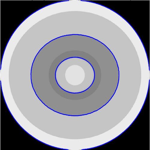
To extent our exploration, we consider images with multi-regional segments in this example. Two images are chosen for this study: image Duck (Figure 8(a), taken from [41]) and image Rings (Figure 9(a), taken from [42]), both are of resolution . The images have at least two or more regions besides the background. In order to obtain the segmentation for multiple regions, we adapt our AMA scheme to perform multi-level segmentations. Metric tensor is used for this example. The results are shown in Figures 8 and 9, respectively.
Two-level AMA segmentation is performed for image Duck (Figure 8(a)). The time step is the same for both levels, that is, . Two iterations are sufficient for the first level, and six iterations are used for the second level. The total computational time is Total-time=15.1s. The results are shown in Figures 8.

(a)

(b)

(c)

(d) first-level

(e) second-level
The first-level AMA segmentation only provides results for the right half of the duck, see Figures 8(b) and (d). Then the second-level AMA segmentation provides results for the left half of the duck, see Figure 8(c). Figure 8(e) shows the result after the second-level segmentation where both regions are combined together. As can be seen from Figure 8(e), the middle part of the duck was treated as background due to its gray value being very close to the background.
For image Rings (Figure 9(a)), the regions are defined by the 6 curves (circles). Three-level AMA segmentation is performed to catch all the curves, and is used in all levels. Two iterations are sufficient for the first level, four iterations are needed for the second level, and seven iterations are used for the third level. The total computational time is Total-time=57s. The results are shown in Figure 9.

(a)
(b)

(c)

(d)

(e)

(f)
The first-level segmentation provides result for two evolved curves as shown in Figures 9(b). The second-level segmentation shows two additional evolved curves from outside region (Figure 9(d)), while evolving inside does not provide any new curve. The third-level segmentation provides two additional evolved curves, one from inside region (Figure 9(e)) and one from outside region (Figure 9(f)). After three levels, we are able to catch all the circles (curves).
5 Conclusions and comments
Partial differential equation (PDE) methods have become a popular method in image segmentation due to its solid mathematical foundation and numerical stability. However, their numerical computations are usually time intensive. Anisotropic mesh adaptation has been successfully used in solving PDEs by many researchers. In this paper, we have introduced a framework of anisotropic mesh adaptation methods (AMA) for image segmentation with the main purpose of improving computational efficiency as well as accuracy.
In our AMA segmentation method, we first represent the image with fewer points (pixels) than the original image using an anisotropic triangular mesh. Then we use the corresponding mesh along with finite element method to solve the PDE model (14) and (2) derived from the minimization of the Mumford-Shah functional.
We have applied the AMA segmentation algorithm to a few test images, and compared the results with those obtained using traditional finite difference schemes (FDS). Images in Examples 4.1 and 4.2 do not have noise and the main features are in one region. Thus one-level AMA segmentation has been performed, and the results are better than those obtained using FDS. Our AMA segmentation scheme is also much faster than FDS.
We have also considered segmentation for a noisy image in Example 4.3. Traditional FDS does not converge unless the image is downscaled to lower resolution. However, our AMA segmentation converges after 4 iterations and takes less than 35s to complete the task. Furthermore, segmentation deals with noise better than segmentation.
Our AMA segmentation algorithm is also adapted to perform multi-level segmentation for images containing multiple regions. The results from Example 4.4 demonstrate the effectiveness of the multi-level AMA segmentation.
In summary, we have introduced an AMA segmentation method that has significant advantage over traditional finite difference schemes in terms of both computational efficiency and segmentation results. AMA segmentation can also deal well with noisy images and images with multiple regions. The method has potential applications in other areas such as medical image segmentation.
References
- [1] L. G. Shapiro and G. C. Stockman. Computer vision: Theory and applications. 2001.
- [2] W. X. Kang, Q. Q. Yang, and R. P. Liang. The comparative research on image segmentation algorithms. In Education Technology and Computer Science, 2009. ETCS’09. First International Workshop on, volume 2, pages 703–707. IEEE, 2009.
- [3] L. Barghout and L. Lee. Perceptual information processing system, March 25 2004. US Patent App. 10/618,543.
- [4] M. Forouzanfar, N. Forghani, and M. Teshnehlab. Parameter optimization of improved fuzzy c-means clustering algorithm for brain mr image segmentation. Engineering Applications of Artificial Intelligence, 23(2):160–168, 2010.
- [5] E. B. George and M. Karnan. Mr brain image segmentation using bacteria foraging optimization algorithm. International journal of engineering and technology (IJET), 4(5):295–301, 2012.
- [6] J. A. Delmerico, P. David, and J. J. Corso. Building facade detection, segmentation, and parameter estimation for mobile robot localization and guidance. In Intelligent Robots and Systems (IROS), 2011 IEEE/RSJ International Conference on, pages 1632–1639. IEEE, 2011.
- [7] L. Wang, X. Duan, Q. Zhang, Z. Niu, G. Hua, and N. Zheng. Segment-tube: Spatio-temporal action localization in untrimmed videos with per-frame segmentation. Sensors, 18(5):1657, 2018.
- [8] J. F. Khan, S. M. Bhuiyan, and R. R. Adhami. Image segmentation and shape analysis for road-sign detection. IEEE Transactions on Intelligent Transportation Systems, 12(1):83–96, 2011.
- [9] A. Janowczyk, R. Chandran, S.and Singh, D. Sasaroli, G. Coukos, M. D. Feldman, and A. Madabhushi. High-throughput biomarker segmentation on ovarian cancer tissue microarrays via hierarchical normalized cuts. IEEE Transactions on Biomedical Engineering, 59(5):1240–1252, 2012.
- [10] Y. J. Zhang. An overview of image and video segmentation in the last 40 years. In Advances in Image and Video Segmentation, pages 1–16. IGI Global, 2006.
- [11] E. A. Anjna and R. K. Er. Review of image segmentation technique. International Journal of Advanced Research in Computer Science, 8(4), 2017.
- [12] M. Wahba. An automated modified region growing technique for prostate segmentation in trans-rectal ultrasound images. Master’s thesis, University of Waterloo, 2009.
- [13] D. Mumford and J. Shah. Optimal approximations by piecewise smooth functions and associated variational problems. Communications on pure and applied mathematics, 42(5):577–685, 1989.
- [14] L. C. Evans. Graduate studies in mathematics, 1998.
- [15] P. Getreuer. Chan-vese segmentation. Image Processing On Line, 2:214–224, 2012.
- [16] P. Perona and J. Malik. Scale-space and edge detection using anisotropic diffusion. IEEE Transactions on pattern analysis and machine intelligence, 12(7):629–639, 1990.
- [17] S. Kichenassamy. The perona–malik paradox. SIAM Journal on Applied Mathematics, 57(5):1328–1342, 1997.
- [18] X. Li. Anisotropic mesh adaptation for image representation. EURASIP Journal on Image and Video Processing, 2016(1):26, 2016.
- [19] G. Aubert and P. Kornprobst. Mathematical problems in image processing: partial differential equations and the calculus of variations, volume 147. Springer Science & Business Media, 2006.
- [20] L. Ambrosio and V. M. Tortorelli. Approximation of functional depending on jumps by elliptic functional via t-convergence. Communications on Pure and Applied Mathematics, 43(8):999–1036, 1990.
- [21] T. F. Chan and L. A. Vese. Active contours without edges/ieee transactions on image processing.-vol. 10 (2)., 2001.
- [22] S. Gao and T. D. Bui. Image segmentation and selective smoothing by using mumford-shah model. IEEE Transactions on Image Processing, 14(10):1537–1549, 2005.
- [23] M. Gage, R. S. Hamilton, et al. The heat equation shrinking convex plane curves. Journal of Differential Geometry, 23(1):69–96, 1986.
- [24] J. A. Sethian. Level set methods and fast marching methods: evolving interfaces in computational geometry, fluid mechanics, computer vision, and materials science, volume 3. Cambridge university press, 1999.
- [25] J. M. Morel and S. Solimini. Variational methods in image segmentation: with seven image processing experiments, volume 14. Springer Science & Business Media, 2012.
- [26] B. Sumengen, B. S. Manjunath, and C. Kenney. Image segmentation using curve evolution and flow fields. In Image Processing. 2002. Proceedings. 2002 International Conference on, volume 1, pages I–I. IEEE, 2002.
- [27] S. Osher and J. A Sethian. Fronts propagating with curvature-dependent speed: algorithms based on hamilton-jacobi formulations. Journal of computational physics, 79(1):12–49, 1988.
- [28] P.J. Frey and F. Alauzet. Anisotropic mesh adaptation for cfd computations. Comput. Methods. Appl. Mech. Engrg., 194:5068–5082, 2005.
- [29] W. Huang and X. Li. An anisotropic mesh adaptation method for the finite element solution of variational problems. Fin. Elem. Anal. Des., 46:61–73, 2010.
- [30] X. Li and W. Huang. An anisotropic mesh adaptation method for the finite element solution of heterogeneous anisotropic diffusion problems. Journal of Computational Physics, 229(21):8072–8094, 2010.
- [31] A. Van Dam and P.A. Zegeling. Balanced monitoring of flow phenomena in moving mesh methods. Commun. Comput. Phys., 7:138–170, 2010.
- [32] X. Li and W. Huang. Maximum principle for the finite element solution of time-dependent anisotropic diffusion problems. Numer. Meth. PDEs, 29:1963–1985, 2013.
- [33] J. Wackers, G. Deng, A. Leroyer, P. Queutey, and M. Visonneau. Adaptive grid refinement for hydrodynamic flows. Computers & Fluids, 55:85–100, 2012.
- [34] X. Li. Anisotropic mesh adaptation for finite element solution of anisotropic porous medium equation. Computers & Mathematics with Applications, 75:2086–2099, 2018.
- [35] W. Huang. Mathematical principles of anisotropic mesh adaptation. Commun. Comput. Phys, 1(2):276–310, 2006.
- [36] W. Huang. Metric tensors for anisotropic mesh generation. Journal of computational physics, 204(2):633–665, 2005.
- [37] J. Wang and W. Huang. Image segmentation with eigenfunctions of an anisotropic diffusion operator. IEEE Transactions on Image Processing, 25(5):2155–2167, 2016.
- [38] F Hecht. Bidimensional anisotropic mesh generator software(bamg), 2010.
- [39] Tatyana Vavrukh. Acute thyroiditis - a rare but insidious thyroid disease. https://schitovidka.su/zabolevaniya/tireoidity/ostryj-tireoidit-487, accessed September 1, 2019.
- [40] Ricardo Longoria. Bow hunting the polar bear. http://bowsite.com/bowsite/features/articles/polarbearricardo/, accessed September 1, 2019.
- [41] Bryan Tyler Parker. Pb-lite: Boundary detection. http://cs.brown.edu/courses/cs143/2011/results/proj2/btparker/, accessed September 1, 2019.
- [42] Ernest Burgess. Concentric zone model. https://en.wikipedia.org/wiki/Concentric_zone_model, accessed September 1, 2019.