Improving key rates of the unbalanced phase-encoded BB84 protocol using the flag-state squashing modelPreprint: APS/123-QED

We start by identifying two equivalent optical models for the Mach-Zehnder component that appears in both Alice’s and Bob’s apparatus. The descriptions for the two models are illustrated in Fig. 2. Instead of having the loss in one arm of the interferometer, the equivalent model places a loss element in front of the Mach-Zehnder component, which then has an asymmetric beam splitter at the entry Ferenczi et al. 2012.

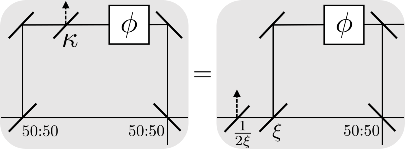
This replacement picture tells us that Alice’s loss can be absorbed into the rescaled amplitude of the incoming single laser pulse, whereas Bob’s loss can be absorbed into the channel’s action.

We use the source-replacement scheme Bennett et al. 1992; Curty et al. 2004 to represent a prepare-and-measure scheme with an entanglement-based scheme. Since Alice’s signal state is mixed, we will introduce a purifying “shield” system that will be left behind in the source so that the existing source-replacement framework can be applied. We will provide a detailed description of the entangled pure state prepared by Alice below.

To prepare the output signal state, Alice’s laser first creates a phase-randomised coherent state

where $p_{n}(\beta)=e^{-|\beta|^{2}}\frac{|\beta|^{2n}}{n!}$ is the Poissonian distribution in photon number $n$. She then sends it through her encoding device set at a phase $\phi_{x}$ which outputs a time-bin signal with two modes,

where $|\psi^{\theta}_{x}(\alpha)\rangle=|\alpha e^{i\theta},\sqrt{\kappa}\;\alpha e^{i(\theta-\phi_{x})}\rangle$.

In the following steps, we will express the state $\sigma_{x}(\alpha)$ in a two-mode Fock basis $\{|s^{x}_{n}(\xi)\rangle\}$ which is defined later in Eqn. (8). Let $\widetilde{a}_{1}^{\;\dagger}$ and $\widetilde{a}_{2}^{\;\dagger}$ be the creation operators of the two output time modes of the signal. We define a rescaled amplitude $\widetilde{\alpha}\coloneqq\alpha\sqrt{1+\kappa}=\alpha/\sqrt{\xi}$ with the definition $\xi\coloneqq\frac{1}{1+\kappa}$ and a new mode creation operator

We define a set of two-mode Fock states for $n\in\mathbb{N}$ as

The state $|\psi^{\theta}_{x}(\alpha)\rangle$ can be rewritten in the new basis as

which is a coherent state with amplitude $\widetilde{\alpha}$. The phase-randomised signal state is therefore a Poissonian mixture of the new Fock states as in

Since the signal state $\sigma_{x}(\alpha)$ is mixed, Alice can purify the state by introducing an ancillary system $A_{S}$ such that the following is a pure state

where the register $A^{\prime}$ is the signal system. Note that the probability $p_{n}(\widetilde{\alpha})$ is independent of Alice’s choice $x$.

We can thus summarise the source description as Alice preparing an entangled pure state

where $\{|x\rangle_{A}\}_{x=0,...,3}$ is an orthonormal basis of Alice’s register $A$ for $x$ corresponding to the phase $\phi_{x}=\frac{\pi}{2}x$ and $p_{x}=\frac{1}{4}$ for all $x\in\{0,1,2,3\}$. Note that registers $A$ and $A_{S}$ are private to Alice, and Eve only has access to the signal system $A^{\prime}$. We call the purifying system $A_{S}$ a “shield” system for it to be inaccessible to Eve (i.e. Eve only gets the mixed state $\sigma_{x}(\alpha)$ but not the pure state $|\sigma_{x}(\alpha)\rangle_{A_{S}A^{\prime}}$).

In the prepare-and-measure scheme, the action of Alice randomly choosing the phase $\phi_{x}$ in the signal state is equivalent to a measurement on $|\Psi\rangle_{AA_{S}A^{\prime}}$ with POVM $\{|x\rangle\langle x|_{A}\}_{x=0,...,3}$. Alice’s measurement can be performed before or after Bob performs his measurement.

We start out by describing the POVM of Bob’s measurement assuming ideal devices, especially without dark counts of the detectors. We will later on derive the POVM of devices with specified dark counts. To characterise all of Bob’s possible measurement outcomes, we construct his POVM using the creation and annihilation operators for six optical modes arriving at 3 different time slots and at 2 detectors. Ignoring global phases, the six annihilation operators of a fixed phase $\phi_{B}$, which correspond to the six “click” locations depicted in Fig. 1, are

where $a_{1}$ and $a_{2}$ are annihilation operators of the two incoming time modes of the signal.

Since $b_{1}=b_{4}$ and $b_{3}=b_{6}$, the POVM elements corresponding to click events at 1 and 4 (3 and 6) are the same. Hence, each pair can be combined into a single time-mode annihilation operator. The corresponding operators for the two pairs are

where $t_{1}$ and $t_{3}$ denote the 1st and 3rd time slots in Fig 1. This is equivalent to coarse-graining the outside-only click POVM elements and outcome probabilities but without losing information about the relative phase, $\phi_{x}-\phi_{B}$. This reduces the redundancy in constraints for the optimisation which will be described in Sec. IV.3.

As Bob’s measurement outcomes consist of all combinations of click events at different time slots, detectors, and basis choices, his POVM elements are obtained by summing weighted projectors of all possible states that could lead to a particular click pattern. Based on the fact that Bob uses threshold detectors for detection, all POVM elements are block-diagonal in total photon number basis Beaudry et al. 2008; Gittsovich et al. 2014.

These allow the construction of Bob’s POVM elements in terms of the modes impinging on the detectors by first restricting to the $n$-total photon subspace of Bob’s entire system, and defining the following operators corresponding to different click events:

• •

  no-click: (for $n=0$)

  $$F_{0}^{\phi_{B}}=p(\phi_{B})|0\rangle\langle 0|,$$

  (18)

• •

  single-click: (for $n\geq 1$)

  $$F^{n,\phi_{B}}_{i_{1}}=p(\phi_{B})\frac{1}{n!}(b_{i_{1}}^{\dagger})^{n}|0\rangle\langle 0|b_{i_{1}}^{n}\;,$$

  (19)

• •

  double-click: (for $n\geq 2$)

  $$F^{n,\phi_{B}}_{i_{1},i_{2}}=p(\phi_{B})\sum_{k=1}^{n-1}\frac{(b_{i_{1}}^{\dagger})^{n-k}(b_{i_{2}}^{\dagger})^{k}|0\rangle\langle 0|b_{i_{1}}^{n-k}\;b_{i_{2}}^{k}}{(n-k)!\;k!}\;,$$

  (20)

• •

  triple-click: (for $n\geq 3$)

  $$F^{n,\phi_{B}}_{i_{1},i_{2},i_{3}}=p(\phi_{B})\sum_{k=1}^{n-2}\;\sum_{j=1}^{n-k-1}|\beta_{3}(n,j,k)\rangle\langle\beta_{3}(n,j,k)|$$

  (21)

  with $|\beta_{3}(n,j,k)\rangle=\frac{(b_{i_{1}}^{\dagger})^{n-k-j}(b_{i_{2}}^{\dagger})^{k}(b_{i_{3}}^{\dagger})^{j}|0\rangle}{\sqrt{(n-k-j)!\;k!\;j!}}$ ,

• •

  all-click: (for $n\geq 4$)

  $$F^{n,\phi_{B}}_{\text{ac}}=p(\phi_{B})\sum_{k=1}^{n-3}\;\sum_{j=1}^{n-k-2}\;\sum_{l=1}^{n-k-j-1}|\beta_{4}(n,j,k,l)\rangle\langle\beta_{4}(n,j,k,l)|$$

  (22)

  with $|\beta_{4}(n,j,k,l)\rangle=\frac{(b_{i_{1}}^{\dagger})^{n-k-j-l}(b_{i_{2}}^{\dagger})^{k}(b_{i_{3}}^{\dagger})^{j}(b_{i_{4}}^{\dagger})^{l}|0\rangle}{\sqrt{(n-k-j-l)!\;k!\;j!\;l!}}$ ,

where $p(\phi_{B})$ is the probability of choosing the phase $\phi_{B}$ and $b_{i_{\mu}}^{\dagger}\in\{b_{t_{1}}^{\dagger},b_{2,\phi_{B}}^{\dagger},b_{5,\phi_{B}}^{\dagger},b_{t_{3}}^{\dagger}\}$ are the mode creation operators for a fixed phase $\phi_{B}$, with $b_{i_{\mu}}^{\dagger}\neq b_{i_{\nu}}^{\dagger}$ for all $\mu\neq\nu$ and $\mu,\nu\in\{1,2,3,4\}$. We can express Bob’s POVM elements in terms of the incoming modes, $a_{1}$ and $a_{2}$, by substituting the final modes with Eqns. (15) – (17).

To obtain Bob’s POVM elements for the full Hilbert space, one simply sums over all contributions from all photon number subspaces to get

where $k$ labels the 16 possible click patterns (Bob’s measurement outcomes) in each of the two measurement bases. For $n$ to be less than the minimum photon number to trigger the click event $k$, $F_{k}^{n}$ is a zero operator. If $k$ is the no-click event, $F_{k}^{n}$ is a zero operator for all $n\geq 1$.

To reduce the number of linearly dependent POVM elements for better numerical performance in calculating key rates ¹¹ 1 As we will point out in Sec. IV.1, the number of POVM elements is related to the dimension of the flag-state subspace. If the two POVM elements are linearly dependent, they are essentially the same constraint for the convex optimisation problem in (39) up to a scaling factor. Therefore, omitting either of the two elements will not affect the optimisation result, but the flag-state subspace dimension will reduce by one. As for all numerical optimisations, the smaller the dimension of the problem, the shorter the runtime., we combine the pairs of $\phi_{B}$-independent POVM elements of the two measurement bases into one by summing the two elements together. This reduces the cardinality of Bob’s POVM from 32 to 28 since the following four click patterns: no-click, $t_{1}$-only, $t_{3}$-only, and $t_{1}\&t_{3}$ are basis-independent.

In a trusted dark-count scenario where dark counts are not controlled by Eve, we incorporate the effect of dark counts into Bob’s POVM by applying a classical post-processing map, $\mathcal{P}$, on Bob’s POVM elements $\{F_{k}\}$. The output of the map is a new POVM $\{P_{k}\}$ with each element corresponding to a linear combination of the original POVM such that $P_{k}=\sum_{i}\mathcal{P}_{k,i}\;F_{i}$ where $\mathcal{P}_{k,i}$ are the matrix elements of the linear map $\mathcal{P}$. We illustrate the action of the map $\mathcal{P}$ with the new POVM elements in Eqns. (43)-(49). Since the map $\mathcal{P}$ acts the same on all photon-number subspaces, it also holds that

The map $\mathcal{P}$ models the effect of dark counts as a classical noise in the sense that for each detector and at each detection time window, a no-click event flips to a click event with probability, $p_{d}$. We can recover Bob’s dark-count free POVM $\{F_{k}\}$ by setting the dark-count probability $p_{d}=0$ in the case with untrusted dark counts.

Overall, we obtain the joint POVM of Alice’s and Bob’s measurements $\{|x\rangle\langle x|_{A}\otimes P_{k}\}$ where $x\in\{0,...,3\}$ and $k\in\{1,...,28\}$ since Bob has 28 coarse-grained outcomes in total if no-click is included.

In order to numerically compute the secure key rate, we need to reduce the dimension of Bob’s state from infinite to finite so that numerical optimisation solvers can be used. Since Bob uses threshold detectors, his POVM elements are block-diagonal, so the qubit squashing model Beaudry et al. 2008; Gittsovich et al. 2014; Ferenczi et al. 2012; Narasimhachar, Varun 2011 can be applied. However, by reassigning the multi-click events to single-click events randomly, the squashing model introduces additional qubit errors to the original data. Instead, the flag-state squashing model Zhang et al. 2020 is used here to circumvent this problem.

We set a finite photon-number cutoff $N_{B}$ and define the $(n$ $\leq$ $N_{B})$- and $(n$ $>$ $N_{B})$-photon subspaces to be two Hilbert spaces containing Fock states of at most $N_{B}$ and at least $N_{B}+1$ photons respectively. The flag-state squashing map $\Lambda$ first projects Bob’s state $\rho$ onto the two subspaces. It then applies an identity map to the projected state $\rho_{n\leq N_{B}}$ and measures the projected state $\rho_{n>N_{B}}$ with the POVM $\{P_{k}\}$ to give the squashed state

Bob’s corresponding flag-state squashed POVM elements are

where $N_{B}$ is a finite-number photon cutoff and $k$ labels Bob’s detection events. The joint POVM of Alice’s and Bob’s measurements in the flag-state squashing model is $\{|x\rangle\langle x|_{A}\otimes\widetilde{P}_{k}\}$ where $x\in\{0,...,3\}$ and $k\in\{1,...,28\}$.

Since the measurement channel acting on the $(n>N_{B})$-photon subspace is entanglement breaking Horodecki et al. 2003, one needs to lower bound $\text{Tr}(\Pi_{n\leq N_{B}}\;\rho)$ with Bob’s measurement statistics to ensure that some entanglement between Alice and Bob is preserved in order for them to establish a secret key Curty et al. 2004. For trusted dark counts, we show in Appendix A that the lower bound for the weight of the $(n\leq N_{B})$-photon signal subspace conditioned on Alice choosing signal $x$ is given by

where the conditional cross-click probability, $p(\text{cc}|x)$, is the sum of the observed probabilities of all events excluding no-click events, events with clicks only in time slot $t_{2}$ (inside-only), and events with clicks only in time slots $t_{1},t_{3}$ (outside-only) given that Alice picks signal $x$. We also show in Appendix A that the bound in (27) is always tighter than the dark-count free bound ($p_{d}=0$) derived by Narashimhachar Narasimhachar, Varun 2011, so we could also obtain a lower bound of the secure key rate using that dark-count free bound. For untrusted dark counts, one simply has to use that bound.

In this article, we prove the security of the protocol against any collective attack. Since the signal states and measurements are permutation invariant between different rounds, the quantum de Finetti theorem Renner 2007 or the postselection technique Christandl et al. 2009 can be applied to uplift our security statement to the security against coherent attacks, which will both lead to the same asymptotic key rate. From that we obtain a composable $\epsilon$-security proof Renner 2005 of the protocol under Eve’s general attacks with the same asymptotic key rate as under the collective attack.

Let $R$ be the key register held by Alice in direct reconciliation, $E$ be Eve’s quantum and classical register, $B$ be Bob’s quantum register, $\overline{B}$ and $\widetilde{B}$ be Bob’s classical registers for his measurement outcomes and announcements respectively. The Devetak-Winter formula Devetak and Winter 2005 for asymptotic secure key rate can be expressed as

where $p_{\text{pass}}$ is the probability of passing the sifting and post-selection steps, $\mathbf{S}$ is the set of all density matrices that satisfy Alice’s and Bob’s joint statistics.

The key rate formula (30) can be converted into an alternative form, as shown in Refs. Coles et al. 2016; Winick et al. 2018, using the relative entropy

where $\mathcal{G}$ and $\mathcal{Z}$ are two maps that will be discussed below. The formula includes a privacy amplification (PA) term as the first term and an error correction term $\delta_{\text{EC}}=f_{\text{EC}}\;H(R|\overline{B})$ with a heuristic classical error-correction efficiency factor $f_{\text{EC}}\geq 1$.

The $\mathcal{G}$ map is a completely positive trace non-increasing map capturing the effects of measurements, sifting, post-selection and announcement on Alice’s and Bob’s joint state, which takes the form Winick et al. 2018; Lin et al. 2019

with the Kraus operators of this protocol defined as

where $\{|0\rangle_{\widetilde{B}},|1\rangle_{\widetilde{B}}\}$ is Bob’s basis announcement bit, $\mathcal{F}_{j}^{B}=\sqrt{\sum_{b\in\mathbf{K}}F_{b,\phi_{B}=\frac{\pi}{2}j}}$ and $\mathbf{K}$ denotes Bob’s post-selected outcomes. The $\mathcal{Z}$ map captures the effect of the key map, and is given by

with register $C$ encapsulates all registers except $R$.

Since Alice is sending a Poissonian mixture of Fock states, Eve can, in principle, perform a QND measurement on Alice’s signal to learn its photon number without disturbing the signal itself. We show in Appendix B that as a direct consequence of this the state $\rho_{AA_{S}B}$ is block-diagonal in Alice’s output photon number $\widetilde{n}$. Therefore, without loss of generality, we can restrict the minimisation in Eqn. (31) to be taken over a smaller set $\mathbf{S}^{\prime}=\{\rho_{AA_{S}B}\in\mathbf{S}:\rho_{AA_{S}B}=\sum_{\widetilde{n}=0}^{\infty}p_{\widetilde{n}}\;|\widetilde{n}\rangle\langle\widetilde{n}|_{A_{S}}\otimes\rho_{AB}^{\widetilde{n}}\}$ where $\{\rho_{AB}^{\widetilde{n}}\}$ are the normalised states conditioned on Alice sending out $\widetilde{n}$ photons. This allows one to split the PA term into a probabilistic combination of PA terms associated with different $\widetilde{n}$ as in

See Appendix B for the proof of the decomposition.

For our analysis, we assume a decoy-state scenario Hwang 2003; Wang 2005; Lo et al. 2005, which means that in addition to the usual signal states, Alice prepares also decoy states that are represented by dephased laser pulses with different intensity levels $|\alpha_{i}|^{2}$. More precisely, we assume for simplicity the infinite-decoy scenario, where a countably infinite number of decoy intensities are used so that a decoy data analysis can reveal to Alice and Bob the conditional probabilities of any observable, where the condition is with respect to Alice’s output photon number $\widetilde{n}$.

These conditional probabilities constrain the feasible set of normalised states $\mathbf{S}_{\widetilde{n}}$ for each of Alice’s output photon number $\widetilde{n}$ independently, which further restricts the minimisation in Eqn. (36) to be taken over a smaller set $\mathbf{S}^{\prime\prime}=\{\rho_{AA_{S}B}\in\mathbf{S}:\rho_{AA_{S}B}=\sum_{\widetilde{n}=0}^{\infty}p_{\widetilde{n}}\;|\widetilde{n}\rangle\langle\widetilde{n}|_{A_{S}}\otimes\rho_{AB}^{\widetilde{n}},$ $\rho_{AB}^{\widetilde{n}}\in\mathbf{S}_{\widetilde{n}}$ $\forall$ ${\widetilde{n}}\in\mathbb{N}\}\subset\mathbf{S}^{\prime}$. Given that the probability distribution $\{p_{\widetilde{n}}\}_{{\widetilde{n}}\in\mathbb{N}}$ is fixed by the intensity of the signal, the minimisation over $\mathbf{S}^{\prime\prime}$ can be pulled into the summation and split into minimisations over individual $\mathbf{S}_{\widetilde{n}}$, resulting in the following key rate formula

We remark that the inclusion of a finite number of decoy states would be a natural extension of this work, in which case the description of each set $\mathbf{S}_{\widetilde{n}}$ would depend on other sets $\{\mathbf{S}_{n^{\prime}}:n^{\prime}\neq\widetilde{n}\}$. Hence, a more careful treatment of the PA term would be needed.

The major benefit of breaking down the PA term into individual minimisations is to avoid the need of keeping the infinite-dimensional shield system $A_{S}$ in the argument of the optimisation as seen in Eqn. (31). Instead of optimising over the set of infinite-dimensional states, we convert our problem into an infinite number of optimisations with finite-dimensional arguments.

Notice that when Alice sends out vacuum (0 photons), Eve learns nothing about Alice’s choice $x$, so each key bit $z\in\{0,1\}$ is equally likely to Eve, which implies that $H(R|E)=H(R)=1$. Therefore, the first term in the summation in Eqn. (37) is equal to $p_{\text{pass}}^{\widetilde{n}=0}$ which is the contribution from Alice sending out vacuum to the probability of passing sifting and post-selection.

By Klein’s inequality, quantum relative entropy is non-negative, i.e. $D(A||B)\geq 0$, for all positive semidefinite matrices $A,B\geq 0$ such that $\text{Tr}(A)\geq\text{Tr}(B)$ Watrous 2018, so $D(\mathcal{G}(\rho_{AB}^{\widetilde{n}})||\mathcal{Z}(\mathcal{G}(\rho_{AB}^{\widetilde{n}})))\geq 0$ $\forall$ $\widetilde{n}\in\mathbb{N}$. Thus, omitting any terms in the summation will only reduce the total value on the right-hand side of Eqn. (37). In fact, omitting an $\widetilde{n}$-photon term is the same as treating all $\widetilde{n}$-photon output signals as being tagged for which the encoded state is fully known to Eve. Since we can only optimise a finite number of terms in the infinite sum, we can truncate the infinite sum at $\widetilde{n}=N_{A}$ where $N_{A}$ is a positive finite integer to obtain a lower bound for the key rate. The choice of $N_{A}=1$ corresponds to the tagging as used in Refs. Ferenczi et al. 2012; Sunohara et al. 2013. We then have the key rate expression as

This allows us to reduce the number of finite-dimensional optimisations from infinity to a finite number that corresponds to the limited computational resources available to us.

The convex optimisation problem corresponding to each PA term in Eqn. (38) can be formulated as

The first line in the constraints demands the shared state $\rho_{AB}^{\widetilde{n}}$ conditioned on Alice sending out $\widetilde{n}$ photons to satisfy Alice’s and Bob’s joint measurement outcome probabilities conditioned on $\widetilde{n}$, which are obtained from the infinite-decoy analysis. The second line lower bounds the weight of $\rho_{AB}^{\widetilde{n}}$ in the $(n\leq N_{B})$-photon subspace by Eqn. (27). The third line demands that Alice’s reduced density matrix is unchanged. The last two lines ensure that $\rho_{AB}^{\widetilde{n}}$ is a valid, normalised density matrix.

Following the procedure in Ref. Winick et al. 2018, the suboptimal solutions to the convex optimisation problem (39) for $1\leq\widetilde{n}\leq N_{A}$ are obtained numerically using the MATLAB optimisation package CVX and the Frank-Wolfe algorithm Frank and Wolfe 1956. These suboptimal solutions infer the upper bound for the individual privacy amplification terms in Eqn. (38). A linearisation of each of the optimisation problems at its suboptimal solution results in a primal semidefinite programming (SDP) problem which can be further converted into a dual SDP problem. Using the CVX numerical solver again, the dual suboptimal solutions for $1\leq\widetilde{n}\leq N_{A}$ provide a reliable lower bound on the whole privacy amplification term.

Solving the convex optimisation problem is computationally demanding in terms of time and memory even if the flag-state squashing model is applied to reduce the dimension of the matrix variables $\rho_{AB}^{\widetilde{n}}$. One can further utilise the structure of the flag-state squashed state as described in Eqn. (25) to reduce the number of complex variables in the allowed matrices $\rho_{AB}^{\widetilde{n}}$. Bob’s flag-state squashed POVM elements also enable us to split multiplications between constraint matrices and the state variable $\rho^{\widetilde{n}}_{AB}$. In addition, the objective function in (39) can be evaluated much faster if the computation is restricted only to the non-zero subspaces in the images of the maps $\mathcal{G}$ and $\mathcal{Z}$. With these three techniques, we managed to reduce the computation time of the convex optimisation by a significant amount. See Appendix C for the technical details.

We utilise the fact that the optimisation problem specified in (39) is independent of the mean photon number $|\alpha|^{2}$ of Alice’s phase-randomised coherent state because the minimisations in Eqn. (37) are over each set $\mathbf{S}_{\widetilde{n}}$ separately. In other words, the choice of $|\alpha|^{2}$ only affects the photon number distribution $\{p_{\widetilde{n}}\}$ and the error-correction term $\delta_{\text{EC}}$ in the key rate formula (38). Therefore, we can maximise the key rate lower bound over the signal intensity $|\alpha|^{2}$ efficiently once we have the dual suboptimal solutions since the error-correction term can be directly calculated from the observables of the corresponding simulation.

We simulate the quantum channel between Alice and Bob with a loss-only channel which is essentially an uneven beam splitter. We also assume that both detectors of Bob have equal detection efficiency $\eta_{\text{det}}$, where each detector can be modelled as a beam splitter with a transmission rate $\eta_{\text{det}}$ followed by an ideal detector. In this simple model, a single parameter $\eta$ which we call the total transmissivity describes the combined loss caused by the following three effects: the inefficiency in the process of coupling the signal light to the optical fibre, the absorption and scattering processes of light in transmission through the fibre, and the detection efficiency of Bob’s threshold detectors.

We also investigate the case where we assume the detection efficiency $\eta_{\text{det}}$ to be outside of Eve’s control, as a trusted, characterised loss element of the receiver. In that case, we keep the beam splitter with transmissivity $\eta_{\text{det}}$ in Bob’s apparatus, which in turn modifies the POVM elements described in Sec. III.3. Bob’s POVM with known detection efficiency can be obtained with a similar approach used in Ref. Zhang et al. 2020.

To simulate our statistics when dark counts are present, we generate the outcome probabilities with Bob’s classically post-processed POVM described in Sec. III.3 and Appendix A, which is associated with a dark-count probability, $p_{d}$, for each detector and at each detection time window.

If dark counts are assumed to be trusted in the sense that they are not in Eve’s control, we use the classically post-processed flag-state POVM $\{\widetilde{P}_{k}\}$ as the constraint matrices in the optimisation problem (39) to calculate the privacy amplification term. This approach guarantees the optimisation problem to be feasible since measurement probabilities correspond directly to a quantum state in the simulation.

However, if we consider untrusted dark counts, that is, if we pessimistically attribute the effect of dark count noise to Eve, the flag-state POVM of dark-count free detectors is used as the optimisation constraint matrices instead. Note that unlike the existence of a physical model for pulling out the equal detection efficiency into the channel, this approach is not covered by any physical equivalence model that allows one to outsource the dark counts to Eve. Therefore, it is possible that no quantum states could have led to the classically post-processed statistics if the measurement is assumed to be dark-count free. In that case, the optimisation problem becomes infeasible due to unphysical constraints. This is what we encounter in some parameter regime of our calculation, as we will point out in the next section.

References

- Bennett (1992) C. H. Bennett, Phys. Rev. Lett. 68, 3121 (1992).
- Townsend (1994) P. D. Townsend, Electronics Letters 30, 809 (1994).
- Hughes et al. (1996) R. J. Hughes, G. G. Luther, G. L. Morgan, and C. Simmons, in Coherence and Quantum Optics VII, edited by J. H. Eberly, L. Mandel, and E. Wolf (Springer US, Boston, MA, 1996) pp. 103–111.
- Li et al. (2009) H.-W. Li, Z.-Q. Yin, Z.-F. Han, W.-S. Bao, and G.-C. Guo, “Security of practical phase-coding quantum key distribution,” (2009), arXiv:0911.2938 [quant-ph] .
- Ferenczi et al. (2012) A. Ferenczi, V. Narasimhachar, and N. Lütkenhaus, Phys. Rev. A 86, 042327 (2012).
- Sunohara et al. (2013) S. Sunohara, K. Tamaki, and N. Imoto, “Blind post-processing for the unbalanced bb84,” (2013), arXiv:1302.1701 [quant-ph] .
- Hwang (2003) W.-Y. Hwang, Phys. Rev. Lett. 91, 057901 (2003).
- Wang (2005) X.-B. Wang, Phys. Rev. Lett. 94, 230503 (2005).
- Lo et al. (2005) H.-K. Lo, X. Ma, and K. Chen, Phys. Rev. Lett. 94, 230504 (2005).
- Gottesman et al. (2004) D. Gottesman, H.-K. Lo, N. Lütkenhaus, and J. Preskill, Quantum Info. Comput. 4, 325–360 (2004).
- Inamori et al. (2007) H. Inamori, N. Lütkenhaus, and D. Mayers, The European Physical Journal D 41, 599 (2007).
- Beaudry et al. (2008) N. J. Beaudry, T. Moroder, and N. Lütkenhaus, Phys. Rev. Lett. 101, 093601 (2008).
- Gittsovich et al. (2014) O. Gittsovich, N. J. Beaudry, V. Narasimhachar, R. R. Alvarez, T. Moroder, and N. Lütkenhaus, Phys. Rev. A 89, 012325 (2014).
- Narasimhachar, Varun (2011) Narasimhachar, Varun, “Study of realistic devices for quantum key-distribution,” (2011).
- Brassard et al. (2000) G. Brassard, N. Lütkenhaus, T. Mor, and B. C. Sanders, Phys. Rev. Lett. 85, 1330 (2000).
- Winick et al. (2018) A. Winick, N. Lütkenhaus, and P. J. Coles, Quantum 2, 77 (2018).
- Zhang et al. (2020) Y. Zhang, P. J. Coles, A. Winick, J. Lin, and N. Lutkenhaus, “Security proof of practical quantum key distribution with detection-efficiency mismatch,” (2020), arXiv:2004.04383 [quant-ph] .
- Lo et al. (2004) H.-K. Lo, H. Chau, and M. Ardehali, Journal of Cryptology 18, 133 (2004).
- Bennett et al. (1992) C. H. Bennett, G. Brassard, and N. D. Mermin, Phys. Rev. Lett. 68, 557 (1992).
- Curty et al. (2004) M. Curty, M. Lewenstein, and N. Lütkenhaus, Phys. Rev. Lett. 92, 217903 (2004).
- (21) As we will point out in Sec. IV.1, the number of POVM elements is related to the dimension of the flag-state subspace. If the two POVM elements are linearly dependent, they are essentially the same constraint for the convex optimisation problem in (39) up to a scaling factor. Therefore, omitting either of the two elements will not affect the optimisation result, but the flag-state subspace dimension will reduce by one. As for all numerical optimisations, the smaller the dimension of the problem, the shorter the runtime.
- Horodecki et al. (2003) M. Horodecki, P. W. Shor, and M. B. Ruskai, Reviews in Mathematical Physics 15, 629 (2003), https://doi.org/10.1142/S0129055X03001709 .
- Renner (2007) R. Renner, Nature Physics 3, 645 (2007).
- Christandl et al. (2009) M. Christandl, R. König, and R. Renner, Phys. Rev. Lett. 102, 020504 (2009).
- Renner (2005) R. Renner, “Security of quantum key distribution,” (2005), arXiv:quant-ph/0512258 [quant-ph] .
- Devetak and Winter (2005) I. Devetak and A. Winter, Proceedings of the Royal Society A: Mathematical, Physical and Engineering Sciences 461, 207 (2005).
- Coles et al. (2016) P. J. Coles, E. M. Metodiev, and N. Lütkenhaus, Nature Communications 7, 11712 (2016).
- Lin et al. (2019) J. Lin, T. Upadhyaya, and N. Lütkenhaus, Phys. Rev. X 9, 041064 (2019).
- Watrous (2018) J. Watrous, The Theory of Quantum Information (Cambridge University Press, 2018).
- Frank and Wolfe (1956) M. Frank and P. Wolfe, Naval Research Logistics Quarterly 3, 95 (1956), https://onlinelibrary.wiley.com/doi/pdf/10.1002/nav.3800030109 .
- Gobby et al. (2004) C. Gobby, Z. L. Yuan, and A. J. Shields, Applied Physics Letters 84, 3762 (2004), https://doi.org/10.1063/1.1738173 .
- Scarani et al. (2009) V. Scarani, H. Bechmann-Pasquinucci, N. J. Cerf, M. Dušek, N. Lütkenhaus, and M. Peev, Rev. Mod. Phys. 81, 1301 (2009).
- George et al. (2020) I. George, J. Lin, and N. Lütkenhaus, “Numerical calculations of finite key rate for general quantum key distribution protocols,” (2020), arXiv:2004.11865 [quant-ph] .