Stability and Complexity Analyses of Finite Difference Algorithms for the Time-fractional Diffusion Equation

Nirupama Bhattacharya Affiliation: Department of Bioengineering
University of California, San Diego Gabriel A. Silva Note: Corresponding author - G.S., Email: gsilva@ucsd.edu Affiliation: Department of Bioengineering
University of California, San Diego Affiliation: Department of Neurosciences
University of California, San Diego Affiliation: Center for Engineered Natural Intelligence
University of California, San Diego

Abstract

Fractional differential equations (FDEs) are an extension of the theory of fractional calculus. However, due to the difficulty in finding analytical solutions, there have not been extensive applications of FDEs until recent decades. With the advent of increasing computational capacity along with advances in numerical methods, there has been increased interest in using FDEs to represent complex physical processes, where dynamics may not be as accurately captured with classical differential equations. The time-fractional diffusion equation is an FDE that represents the underlying physical mechanism of anomalous diffusion. But finding tractable analytical solutions to FDEs is often much more involved than solving for the solutions of integer order differential equations, and in many cases it is not possible to frame solutions in a closed form expression that can be easily simulated or visually represented. Therefore the development of numerical methods is vital. In previous work we implemented the full 2D time-fractional diffusion equation as a Forward Time Central Space finite difference equation by using the Grünwald-Letnikov definition of the fractional derivative. In addition, we derived an adaptive time step version that improves on calculation speed, with some tradeoff in accuracy. Here, we explore and characterize stability of these algorithms, in order to define bounds on computational parameters that are crucial for performing accurate simulations. We also analyze the time complexity of the algorithms, and describe an alternate adaptive time step approach that utilizes a linked list implementation, which yields better algorithmic efficiency.

1 Introduction

Fractional calculus as a mathematical field has existed almost as long as classical integer-order calculus, much of the theory having been developed by Liouville, Laplace, Fourier, Euler, Lagrange, Riemann, and others [12, 8]. Analogous to ordinary and partial differential equations being used to model physical phenomena using classical calculus, fractional differential equations (FDEs) are an extension of the theory of fractional calculus. However, due to the difficulty in finding analytical solutions to FDEs, there have not been extensive applications of these equations until recent decades. With the advent of increasing computational capacity along with advances in numerical methods, there has been increased interest in using FDEs to represent complex physical processes, where dynamics may not be as accurately captured with classical differential equations.

Fractional differential equations have been useful for modeling such varied applications as advection-dispersion transport phenomena [1], wave propagation in bone and other rigid porous materials [14, 3], viscoelasticity [15], edge detection in image processing [10], and neurodynamics and modeling of signal processing in neuronal dendrites [5]. Richard Magin discusses a wide array of fractional calculus modeling applications in the field of bioengineering alone, including signaling across membranes, feedback control in neural systems, neurodynamics, capacitor and dielectric models, the behavior of viscoelastic materials, circuit models of electrode interfaces, cell biomechanics, and electrochemistry, among many other applications [8, 9].

In particular, the time-fractional diffusion equation is an FDE that represents the underlying physical mechanism of anomalous diffusion. In the same way that the classical diffusion equation can be derived from statistical analysis of particle interactions, one can also show how the micromolecular behavior of particles can, under a different set of fundamental statistical assumptions, be represented on a macro scale in two dimensions by the fractional diffusion equation of the form [2]:

\frac{\partial^{\gamma}u(\vec{x},t)}{\partial t^{\gamma}}=\alpha\frac{\partial^{2}u(\vec{x},t)}{\partial x^{2}}+\beta\frac{\partial^{2}u(\vec{x},t)}{\partial y^{2}}

(1.1)

where $\gamma<1$ denotes the subdiffusion regime, $\gamma=1$ denotes classical Gaussian diffusion, $\gamma>1$ denotes the superdiffusion regime, and $\alpha$ and $\beta$ represent the diffusion coefficients in the $x$ and $y$ directions, respectively (in $\frac{spatial\;unit^{2}}{time\;unit^{\gamma}}$ ).

Finding tractable analytical solutions to FDEs like Eq. 1.1 is often much more involved than solving for the solutions of integer order differential equations, and in many cases it is not possible to frame solutions in a closed form expression that can be easily simulated or visually represented. Therefore the development of numerical methods is vital. Over the last decade there have been numerous algorithms developed for FDEs like the time-fractional diffusion equation, and there is often a tradeoff between calculation speed and efficiency, complexity, stability, and accuracy. In [7] we walk through the discretization of Eq. 1.1 into the full two-dimensional fractional FTCS (Forward Time Central Space) finite difference equation, making use of the Grünwald-Letnikov definition of the fractional derivative, which allows us to use a discrete summation in our numerical algorithm. We also derive an adaptive time step algorithm which builds on the foundation of the full 2D fractional FTCS equation but improves calculation speed and efficiency, while maintaining accuracy [7]. However, both the FTCS equation and adaptive algorithms are explicit methods with a limited stability regime. Here we fully explore and characterize the stability of these two finite difference schemes in order to define bounds on important computational parameters like time step and spatial discretization and grid size; selecting these parameters appropriately is crucial for performing accurate simulations.

There are numerous approaches to analyzing the stability of finite difference schemes, including modified wavenumber analysis, matrix eigenvalue analysis, and other more mathematically complex methods derived from stability definitions involving matrix norms. Several methods, including matrix analysis, are widely applicable but sometimes impossible to approach analytically or without the aid of iterative procedures. However, since our numerical algorithms are both fully discretized in space and time, and linear with constant coefficients (in their homogeneous versions), we show in the next section that an appropriate choice is a von Neumann stability analysis. We assume the general solution at an arbitrary location and time step is a linear combination of special solutions, represented by a function that is separable in its temporal and spatial variables. We find that our stability analysis and expressions of parameter bounds agree very well with our results, where we simulate several examples with various parameter combinations.

In addition to stability analysis, a complexity analysis is another important metric used to characterize the efficiency of numerical algorithms, as measured by execution time of the algorithm as a function of some input variable. In the case of the algorithms described in this paper, we are interested in how the execution time varies with $N_{x},\;N_{y}$ (grid size of the simulation in the x and y directions, respectfully), or $N$ , the number of timesteps. The relationship between execution time and input variable is usually given in Big- $O$ notation using a worst case scenario, or average case scenario which is often a better reflection of the average behavior of the algorithm run time. In Section 3, we explore the time complexity of the same two algorithms for which we complete the stability analysis, and in addition, analyze an alternate version of the adaptive timestep algorithm that involves a linked list implementation (introduced in [7]) that yields better algorithmic efficiency. For mathematical simplicity we analyze our algorithms according to worst case scenarios and interpret the results as a proof of bounding behavior - the actual run time of the algorithms may be more efficient, but never less efficient. We also present simulated data that verifies our theoretical complexity analyses.

2 Stability Analysis of the Two-dimensional Fractional FTCS Discretization

2.1 Full Implementation

We begin by considering the circumstances under which the 2D fractional FTCS finite difference equation is stable, and consider the advantages and disadvantages of several different analytical approaches. We restate the FTCS discretized equation in two dimensions (see [7, 2] for more details):

$\displaystyle u_{j,l}^{n+1}-u_{j,l}^{n}$	$\displaystyle=$	$\displaystyle\Delta_{t}^{\gamma}\sum_{m=0}^{n}\psi(\gamma,m)\left(\frac{\alpha}{\Delta x^{2}}\delta x_{j,l}^{n-m}+\frac{\beta}{\Delta y^{2}}\delta y_{j,l}^{n-m}\right)$	(2.1)
$\displaystyle\delta x_{j,l}^{n}$	$\displaystyle=$	$\displaystyle u_{j+1,l}^{n}-2u_{j,l}^{n}+u_{j-1,l}^{n}$
$\displaystyle\delta y_{j,l}^{n}$	$\displaystyle=$	$\displaystyle u_{j,l+1}^{n}-2u_{j,l}^{n}+u_{j,l-1}^{n}$

where $\Delta_{t}$ is the time step, and $\Delta x$ and $\Delta y$ are spatial grid discretizations in the x and y directions. Our spatial range is

u_{j,l}^{n}\mid j=0,1,2,...,N_{x}-1;\;l=0,1,2,...,N_{y}-1

and

u_{j,l}^{n}\mid j=0,N_{x}-1;\;l=0,N_{y}-1

denotes the boundary points. $\psi\left(\gamma,m\right)$ , which we refer to as a ‘memory function’, represents a binomial term $\left(-1\right)^{m}\left(\begin{array}[]{c}1-\gamma\\ m\end{array}\right)$ , and results from the use of the Grünwald-Letnikov definition of the fractional derivative, as discussed in [7, 13, 2].

2.1.1 Matrix Stability Analysis

Matrix stability analysis is a method of analysis that can be applied to any problem without particular assumptions or constraints on coefficients, and includes the effects of boundary conditions [11]. We would like to reformulate Eq. 2.1 into a matrix equation in the form $W_{n+1}=L_{n}W_{n}+f_{n}$ where the $W$ matrices hold $u$ values at times $n+1$ and $n$ , the $L_{n}$ matrix represents the difference operator at time $n$ , and $f_{n}$ is a constant vector that takes into account boundary conditions at time step $n$ (here we assume boundary conditions are known for all timesteps).

For example, for $n=0$ , Eq. 2.1 becomes:

u_{j,l}^{1}=u_{j,l}^{0}+\Delta_{t}^{\gamma}\psi(\gamma,0)\left(\frac{\alpha}{\Delta x^{2}}\delta x_{j,l}^{0}+\frac{\beta}{\Delta y^{2}}\delta y_{j,l}^{0}\right)

Then the matrix equation is formulated as follows. We order grid values $u$ into a vector (excluding the boundary points) such that $W$ at some time step $n$ is

W_{n}=\left[\begin{array}[]{c}u_{1,1}\\ u_{1,2}\\ u_{1,3}\\ \vdots\\ u_{1,N_{y}-2}\\ \vdots\\ u_{N_{x}-2,1}\\ u_{N_{x}-2,2}\\ \vdots\\ u_{N_{x}-2,N_{y}-2}\end{array}\right]^{n}

(2.2)

For $n=0$ our matrix equation now becomes $W_{1}=L_{0}W_{0}+f_{0}$ where the matrix $L_{0}$ accounts for interior non-boundary grid points and consists of block matrices $T_{0}$ (a tridiagonal matrix) and $R_{0}$ (a diagonal matrix):

$\displaystyle L_{0}$	$\displaystyle=$	$\displaystyle\left[\begin{array}[]{ccccc}T_{0}&R_{0}&0&\cdots&0\\ R_{0}&T_{0}&\ddots&\ddots&\vdots\\ 0&R_{0}&\ddots&R_{0}&0\\ \vdots&\ddots&\ddots&T_{0}&R_{0}\\ 0&\cdots&0&R_{0}&T_{0}\end{array}\right]$
$\displaystyle T_{0}$	$\displaystyle=$	$\displaystyle\left[\begin{array}[]{ccccc}1-2r_{x}\psi\left(\gamma,0\right)-2r_{y}\psi\left(\gamma,0\right)&r_{y}\psi(\gamma,0)&0&\cdots&0\\ r_{y}\psi(\gamma,0)&&\ddots&\ddots&\vdots\\ 0&\ddots&\ddots&&0\\ \vdots&\ddots&&&r_{y}\psi(\gamma,0)\\ 0&\cdots&0&r_{y}\psi(\gamma,0)&1-2r_{x}\psi\left(\gamma,0\right)-2r_{y}\psi\left(\gamma,0\right)\end{array}\right]$
$\displaystyle R_{0}$	$\displaystyle=$	$\displaystyle\left[\begin{array}[]{cccc}r_{x}\psi(\gamma,0)&0&\cdots&0\\ 0&\ddots&\ddots&\vdots\\ \vdots&\ddots&\ddots&0\\ 0&\cdots&0&r_{x}\psi(\gamma,0)\end{array}\right]$

where $r_{x}=\frac{\alpha\Delta_{t}^{\gamma}}{\Delta x^{2}}$ and $r_{y}=\frac{\beta\Delta_{t}^{\gamma}}{\Delta y^{2}}$ . $L_{0}$ is size $(N_{x}-2)(N_{y}-2)$ by $(N_{x}-2)(N_{y}-2)$ . $T_{0}$ and $R_{0}$ are each of size $(N_{y}-2)$ by $(N_{y}-2)$ . $f_{0}$ takes into account the boundary points and is a column vector of constants.

For $n=1$ we now must take into account multiple past time points, and our matrix equation becomes

$\displaystyle W_{2}$	$\displaystyle=$	$\displaystyle L_{1}W_{0}+L_{0}W_{1}+f_{01}$
$\displaystyle L_{1}$	$\displaystyle=$	$\displaystyle\left[\begin{array}[]{ccccc}T_{1}&R_{1}&0&\cdots&0\\ R_{1}&T_{1}&\ddots&\ddots&\vdots\\ 0&R_{1}&\ddots&R_{1}&0\\ \vdots&\ddots&\ddots&T_{1}&R_{1}\\ 0&\cdots&0&R_{1}&T_{1}\end{array}\right]$
$\displaystyle T_{1}$	$\displaystyle=$	$\displaystyle\left[\begin{array}[]{ccccc}-2r_{x}\psi\left(\gamma,1\right)-2r_{y}\psi\left(\gamma,1\right)&r_{y}\psi(\gamma,1)&0&\cdots&0\\ r_{y}\psi(\gamma,1)&&\ddots&\ddots&\vdots\\ 0&\ddots&\ddots&&0\\ \vdots&\ddots&&&r_{y}\psi(\gamma,1)\\ 0&\cdots&0&r_{y}\psi(\gamma,1)&-2r_{x}\psi\left(\gamma,1\right)-2r_{y}\psi\left(\gamma,1\right)\end{array}\right]$
$\displaystyle R_{1}$	$\displaystyle=$	$\displaystyle\left[\begin{array}[]{cccc}r_{x}\psi(\gamma,1)&0&\cdots&0\\ 0&\ddots&\ddots&\vdots\\ \vdots&\ddots&\ddots&0\\ 0&\cdots&0&r_{x}\psi(\gamma,1)\end{array}\right]$

and where $f_{01}$ is a column vector that takes into account the boundary conditions from timesteps $0$ and $1$ . We can repurpose this multistep matrix equation into a single step equation:

	$\displaystyle W_{combined,2}$	$\displaystyle=$	$\displaystyle L_{combined,1}W_{combined,1}+f_{01}\;\mbox{with}$
	$\displaystyle W_{combined,2}$	$\displaystyle=$	$\displaystyle\left[\begin{array}[]{c}W_{2}\\ W_{1}\end{array}\right],\;W_{combined,1}=\left[\begin{array}[]{c}W_{1}\\ W_{0}\end{array}\right],\;L_{combined,1}=\left[\begin{array}[]{cc}L_{0}&L_{1}\\ I&0\end{array}\right]$

and $I$ is simply the identity matrix. For $n=2$ the complexity of the matrices involved continues to grow with

	$\displaystyle W_{combined,3}$	$\displaystyle=$	$\displaystyle L_{combined,2}W_{combined,2}+f_{012}$
	$\displaystyle\left[\begin{array}[]{c}W_{3}\\ W_{2}\\ W_{1}\end{array}\right]$	$\displaystyle=$	$\displaystyle\left[\begin{array}[]{ccc}L_{0}&L_{1}&L_{2}\\ I&0&0\\ 0&I&0\end{array}\right]\left[\begin{array}[]{c}W_{2}\\ W_{1}\\ W_{0}\end{array}\right]+f_{012}$

where $L_{0},L_{1},L_{2}...$ are block matrices which consist of tridiagonal and diagonal sub-matrices, as demonstrated in previous steps. In general, we have

$\displaystyle W_{combined,n+1}$	$\displaystyle=L_{combined,n}W_{combined,n}+f_{0...n}$	(2.11)
$\displaystyle W_{combined,n+1}$	$\displaystyle=\left[\begin{array}[]{c}W_{n+1}\\ \vdots\\ \vdots\\ \vdots\\ W_{1}\end{array}\right]$
$\displaystyle L_{combined,n}$	$\displaystyle=\left[\begin{array}[]{ccccc}L_{0}&L_{1}&\cdots&L_{n-1}&L_{n}\\ I&0&&\cdots&0\\ 0&\ddots&\ddots&&\vdots\\ \vdots&\ddots&\ddots&\ddots\\ 0&\cdots&0&I&0\end{array}\right]$
$\displaystyle L_{n}$	$\displaystyle=\left[\begin{array}[]{ccccc}T_{n}&R_{n}&0&\cdots&0\\ R_{n}&T_{n}&\ddots&\ddots&\vdots\\ 0&R_{n}&\ddots&R_{n}&0\\ \vdots&\ddots&\ddots&T_{n}&R_{n}\\ 0&\cdots&0&R_{n}&T_{n}\end{array}\right]$
$\displaystyle T_{n}$	$\displaystyle=\left[\begin{array}[]{ccccc}-2r_{x}\psi\left(\gamma,n\right)-2r_{y}\psi\left(\gamma,n\right)&r_{y}\psi(\gamma,n)&0&\cdots&0\\ r_{y}\psi(\gamma,n)&&\ddots&\ddots&\vdots\\ 0&\ddots&\ddots&&0\\ \vdots&\ddots&&&r_{y}\psi(\gamma,n)\\ 0&\cdots&0&r_{y}\psi(\gamma,n)&-2r_{x}\psi\left(\gamma,n\right)-2r_{y}\psi\left(\gamma,n\right)\end{array}\right],\text{for }n\geq 1$
$\displaystyle R_{n}$	$\displaystyle=\left[\begin{array}[]{cccc}r_{x}\psi(\gamma,n)&0&\cdots&0\\ 0&\ddots&\ddots&\vdots\\ \vdots&\ddots&\ddots&0\\ 0&\cdots&0&r_{x}\psi(\gamma,n)\end{array}\right]$

The goal with matrix stability analysis is to show that for a matrix problem Eq. 2.11, the spectral radius $\rho(L_{combined,n})$ of the difference matrix $L_{combined,n}$ , (i.e., the modulus of its largest eigenvalue) is bounded, usually by 1 [4]. This involves finding the maximum eigenvalue for $L_{combined,n}$ , for all timesteps $n$ , and proving that its modulus is $\leq 1$ . The matrix $L_{combined,n}$ is quite complex and is not in the form of a special matrix where there are known analytical algorithms to find the eigenvalues. This makes the process of finding the eigenvalues very complicated and most likely beyond the realm of an analytic solution, so we consider this to be outside the scope of this paper, and conclude that despite the difficulty of finding the spectral radius, a major advantage of this method would be its generality - it could be applied to any set of boundary conditions, or schemes with non-constant coefficients.

2.1.2 Von Neumann Analysis

As we saw in the previous section, matrix stability analysis for complex algorithms with no simplifying assumptions, requires methods for finding eigenvalues, possibly including iterative numerical schemes. However, our finite difference scheme in Eq. 2.1 has the advantage of being linear with constant coefficients (i.e. $\alpha,\beta$ don’t depend on $t$ or $\vec{x}$ ) on a uniformly spaced grid. With an additional simplifying assumption of periodic boundary conditions, we can make use of von Neumann stability analysis and Fourier series expansion. While von Neumann analysis doesn’t take into account boundary conditions in the same way matrix stability analysis does, we make the reasonable assumption that stability issues are mostly affected by discretization of differential equations inside the domain, and minimally affected by boundary conditions [11]. In the majority of modeling and simulation problems in engineering, we consider this to be a valid and applicable simplifying assumption.

Given our linear scheme with constant coefficient and periodic boundary conditions, we assume the solution of scheme 2.1 at a particular location and time point, can be expressed as a discrete finite complex Fourier series expansion:

\displaystyle u_{j,l}^{n}

\displaystyle=

\displaystyle\sum_{d=0}^{N_{y}-1}\sum_{c=0}^{N_{x}-1}A_{cd}^{n}e^{ik_{c}x_{j}}e^{ik_{d}y_{l}}

(2.34)

where $A_{cd}^{n}$ are the Fourier mode amplitudes, $x_{j}=j\Delta x,\;j=0,1,...,N_{x}-1,y_{l}=l\Delta y,\;l=0,1,...,N_{y}-1$ , and $k_{c}$ and $k_{d}$ are the spatial wavenumbers in the $x$ and $y$ directions, respectively. The wavenumbers represent spatial frequency and are related to wavelength by $\lambda_{x}=\frac{2\pi}{k_{c}},\;\lambda_{y}=\frac{2\pi}{k_{d}}$ . In the context of Fourier modes and stability analysis, we are interested in suppressing (or as we shall see later in this section, limiting the amplification factor of) the high frequency modes (represented by wavelengths on the order of grid sizes $\Delta x$ and $\Delta y$ , and wavenumber values away from $0$ ) because these modes have a low probability of corresponding to any real features of the true solution, and usually represent noise arising from finite precision arithmetic for numerical calculations. The time evolution of each Fourier mode is determined by the same time marching scheme as the full solution $u_{j,l}^{n}$ . And since no Fourier mode can be allowed to increase unbounded in time, we can single out any arbitrary harmonic $A_{cd}^{n}e^{ik_{c}x_{j}}e^{ik_{d}y_{l}}$ and substitute this form into Eq. 2.1 [6]. We utilize the relationships $x_{j+1}=x_{j}+\Delta x,\;x_{j-1}=x_{j}-\Delta x,\;y_{l+1}=y_{l}+\Delta y\;\mbox{and $y_{l-1}=y_{l}-\Delta y$}$ , as well as Euler’s formula and half angle trigonometric identities, to obtain

\displaystyle A_{cd}^{n+1}-A_{cd}^{n}+\Delta_{t}^{\gamma}\left(\frac{4\alpha}{\Delta x^{2}}sin^{2}\left(\frac{k_{c}\Delta x}{2}\right)+\frac{4\beta}{\Delta y^{2}}sin^{2}\left(\frac{k_{d}\Delta y}{2}\right)\right)\sum_{m=0}^{n}\psi\left(\gamma,m\right)A_{cd}^{n-m}=0

(2.35)

If we make the assumption that $A_{cd}$ is independent of time step, we can write

A_{cd}^{n+1}=\sigma_{cd}A_{cd}^{n}

(2.36)

where $\sigma_{cd}$ is known as the amplification factor that gives the growth or decay for Fourier mode $\left(c,d\right)$ . We require $\left|\sigma_{cd}\right|\leq 1$ for all Fourier modes, or else some modes will be amplified at every time step and dominate the solution. We divide Eq. 2.36 by $A_{cd}^{n}$ and rearrange to get

\sigma_{cd}=1-\Delta_{t}^{\gamma}\left(\frac{4\alpha}{\Delta x^{2}}sin^{2}\left(\frac{k_{c}\Delta x}{2}\right)+\frac{4\beta}{\Delta y^{2}}sin^{2}\left(\frac{k_{d}\Delta y}{2}\right)\right)\sum_{m=0}^{n}\psi\left(\gamma,m\right)\sigma_{cd}^{-m}

We require $\left|\sigma_{cd}\right|\leq 1$ for all values of $\sigma_{cd}$ , which are the roots of this polynomial. We can also see that the difficulty of solving for the roots increases as time progresses and $n$ increases. Past the first few timesteps, solving for the roots of the polynomial requires iterative matrix procedures and does not result in a tractable analytical solution from which we can find the bounds on the relationship between $\alpha,\beta,\Delta t,\Delta x,\mbox{and }\Delta y$ . Instead of solving for roots, we will approach the problem by considering ‘worst-case’ scenarios to simplify our expression, and proceed in a similar manner as Yuste and Acedo’s treatment of the analogous one-dimensional case [16]. Consider the bound on the parameters resulting from the case $\sigma_{cd}=1$ :

0\geq\Delta_{t}^{\gamma}\left(\frac{4\alpha}{\Delta x^{2}}sin^{2}\left(\frac{k_{c}\Delta x}{2}\right)+\frac{4\beta}{\Delta y^{2}}sin^{2}\left(\frac{k_{d}\Delta y}{2}\right)\right)\sum_{m=0}^{n}\psi\left(\gamma,m\right)

(2.37)

The summation term and parameters are always greater than $0$ , and therefore Eq. 2.37 can only hold true if both wavenumbers are $0$ (a constant function). Therefore, we consider the other ‘worst-case’ scenario, where $\sigma_{cd}=-1$ :

2=\Delta_{t}^{\gamma}\left(\frac{4\alpha}{\Delta x^{2}}sin^{2}\left(\frac{k_{c}\Delta x}{2}\right)+\frac{4\beta}{\Delta y^{2}}sin^{2}\left(\frac{k_{d}\Delta y}{2}\right)\right)\sum_{m=0}^{n}\psi(\gamma,m)\left(-1\right)^{m}

(2.38)

From Eq. 2.38 we can infer the inequality bounding the parameters as

\Delta_{t}^{\gamma}\left(\frac{4\alpha}{\Delta x^{2}}sin^{2}\left(\frac{k_{c}\Delta x}{2}\right)+\frac{4\beta}{\Delta y^{2}}sin^{2}\left(\frac{k_{d}\Delta y}{2}\right)\right)\leq\frac{2}{\sum_{m=0}^{n}\psi(\gamma,m)\left(-1\right)^{m}}=B_{1}\left(\gamma,n\right)

(2.39)

We can see that the bounded value is dependent on the time step $n$ but the dependence is very weak. Yuste and Acedo demonstrate that in the limit $n\rightarrow\infty$ , the summation term in Eq. 2.39 involving the memory function, is an alternating converging series; as $n$ increases, $B_{1}$ oscillates but clearly converges to an equilibrium value [16]. Therefore we can approximate $\sum_{m=0}^{n}\psi(\gamma,m)\left(-1\right)^{m}$ by taking the limit as $n\rightarrow\infty$ . In [7] we originally derived the 2D FTCS full finite difference equation and adaptive memory algorithms by using the Grünwald-Letnikov definition to make a first-order approximation of the Riemann-Liouville fractional derivative operator [13]. And in the first-order approximation, the memory function $\psi(\gamma,m)$ is defined as $\left(-1\right)^{m}\left(\begin{array}[]{c}1-\gamma\\ m\end{array}\right)$ . Podlubny ([13]) shows that this expression can also be defined as the coefficients of the power series for the function $\left(1-z\right){}^{1-\gamma}:$

\left(1-z\right)^{1-\gamma}=\sum_{m=0}^{\infty}\left(-1\right)^{m}\left(\begin{array}[]{c}1-\gamma\\ m\end{array}\right)z^{m}=\sum_{m=0}^{\infty}\psi(\gamma,m)z^{m}

(2.40)

Applying this identity to $B_{1}\left(\gamma,n\right)$ and considering the limit $n\rightarrow\infty$ , we can derive

B_{2}\left(\gamma\right)=2^{\gamma}

(2.41)

As Yuste and Acedo describe in their considerations of stability in the one-dimensional case, we could consider the second-order approximation of the Riemann-Liouville definition by making use of a different set coefficients to define our memory function. This option would result in a slightly lower bound on our parameters, but for the purposes of estimating appropriate parameter values, we consider the first-order approximation to be sufficient.

From (2.39) we can see that we have three degrees of freedom in parameters that we are free to choose for our simulations : $\Delta_{t},\;\Delta x^{2},\;\Delta y^{2}$ . To determine the most conservative bounds on those degrees of freedom (minimum values for grid size and maximum value for time step), we assume the maximum possible value for the trigonometric terms, $sin^{2}\left(\frac{k_{c}\Delta x}{2}\right)=sin^{2}\left(\frac{k_{d}\Delta y}{2}\right)=1$ . The resulting inequality determining parameter bounds is

\Delta_{t}^{\gamma}\left(\frac{4\alpha}{\Delta x^{2}}+\frac{4\beta}{\Delta y^{2}}\right)\leq B_{2}\left(\gamma\right)

If we assume a simple case with a square grid ( $\Delta x=\Delta y=\Delta)$ and equal diffusion coefficients in both spatial directions $\left(\alpha=\beta\right)$ , the expression becomes

r=\frac{\alpha\Delta t^{\gamma}}{\Delta^{2}}\leq\frac{B_{2}(\gamma)}{8}=2^{\gamma-3}=B_{full}\left(\gamma\right)

(2.42)

As a final check, when we set $\gamma=1$ (classical diffusion), we recover the well known traditional bound $r\leq\frac{1}{4}$ that results from the classical 2D diffusion equation using the FTCS discretization.

2.1.3 Error Propagation

An alternative approach to stability is to consider roundoff error from floating point or finite precision arithmetic, and ensure that this does not propagate in time by requiring error $\left|\epsilon_{j,l}^{n+1}\right|\leq\left|\epsilon_{j,l}^{n}\right|$ . A mathematical derivation based on this interpretation would progress in much the same manner as in Section 2.1.2 and result in similar parameter boundaries.

2.2 Adaptive Memory Algorithm

As discussed in [7], while the full implementation represented by Eq. 2.1 is an accurate finite difference approximation to the solution of Eq. 1.1, using the Grünwald-Letnikov definition of the fractional derivative involves a summation that takes into account the entire past history of the simulation. As the simulation progresses, calculating the summation term becomes increasingly cumbersome, time consuming, and memory intensive. Therefore we have developed an adaptive memory method (introduced in [7]) that improves on computational efficiency while maintaining a level of accuracy comparable to the original full implementation. This is achieved by recognizing that the further back a time point is in the history of the simulation, the less it contributes to the calculation of the solution at the next time point. Therefore we sample the history of the system more frequently for recent time points (which contribute more to the solution at the next time step) and less often for time points further back in the history of the system, weighted by an appropriate amount to compensate for less frequent sampling; this approach significantly reduces actual computational time. For smooth functions, the convolution of $\psi\left(\gamma,m\right)$ and the function in question changes slowly enough that the weighting of the sampled time points compensates for the less frequent sampling, and maintains overall accuracy. The motivation and derivation of this adaptive algorithm is discussed in further detail in [7]. Here we reproduce a modified version of the algorithm and recognize that analyzing stability requires only a few modifications from the process described in the last section.

$\displaystyle\frac{u_{j,l}^{n+1}-u_{j,l}^{n}}{\Delta_{t}^{\gamma}}$	$\displaystyle=$	$\displaystyle\sum_{m=0}^{a}\overbrace{\psi(\gamma,m)\left(\frac{\alpha}{\Delta x^{2}}\delta x_{j,l}^{n-m}+\frac{\beta}{\Delta y^{2}}\delta y_{j,l}^{n-m}\right)}^{R1}$	(2.43)
		$\displaystyle+\sum_{s=2}^{s_{max}(n)}\left\{\sum_{\eta=1}^{\eta_{max}\left(s,n\right)}\overbrace{\left(2s-1\right)\psi\left(\gamma,M\left(s,\eta\right)\right)\left(\frac{\alpha}{\Delta x^{2}}\delta x_{j,l}^{n-M(s,\eta)}+\frac{\beta}{\Delta y^{2}}\delta y_{j,l}^{n-M(s,\eta)}\right)}^{R2}\right.$
		$\displaystyle+\left.\sum_{p=M(s,\eta_{max})+s}^{min(a^{s},n)}\overbrace{\psi(\gamma,p)\left(\frac{\alpha}{\Delta x^{2}}\delta x_{j,l}^{n-p}+\frac{\beta}{\Delta y^{2}}\delta y_{j,l}^{n-p}\right)}^{R3}\right\}$
$\displaystyle M\left(s,\eta\right)$	$\displaystyle=$	$\displaystyle a^{s-1}+\left(2s-1\right)\eta-s+1$
$\displaystyle\eta_{max}\left(s,n\right)$	$\displaystyle=$	$\displaystyle min\left(\left\lfloor\frac{a^{s}-a^{s-1}}{2s-1}\right\rfloor,\left\lfloor\frac{n-a^{s-1}}{2s-1}\right\rfloor\right)$
$\displaystyle\delta x_{j,l}^{n}$	$\displaystyle=$	$\displaystyle u_{j+1,l}^{n}-2u_{j,l}^{n}+u_{j-1,l}^{n}$
$\displaystyle\delta y_{j,l}^{n}$	$\displaystyle=$	$\displaystyle u_{j,l+1}^{n}-2u_{j,l}^{n}+u_{j,l-1}^{n}$	(2.44)

where $a$ is the predefined base interval, $\left\lfloor\;\right\rfloor$ denotes the floor function, and $s_{max}$ is determined by the current time step $n$ such that $a^{s_{max}-1}+1\leq n\leq a^{s_{max}}$ . The terms $R1,R2,R3$ are referred to in more detail during the complexity analysis in later sections.

There are various ways to interpret how $a$ is translated into a numerical algorithm, depending on whether one assumes that it is with respect to $m$ (mathematical series beginning at 0), time step $n$ (which may need to be adjusted to begin from index 0 or 1, depending on the programming language), or time $t$ . For example, if one assumes $a$ is a time, we can define $a_{effective}=a/dt$ where $a$ is converted to a time step. For $dt<1$ this has the same effect as increasing $a$ and interpreting it with respect to time step $n$ . The larger the value of $a$ , the more accurate the scheme presented in Eq. 2.43, when compared against the full algorithm in Eq. 2.1. Fig. 2.1 shows the error plots where the adaptive step algorithm in Eq. 2.43 is compared against the full implementation (the reference case) Eq. 2.1, for the adaptive step parameter values $a=4$ and $a=20$ . Note that the initial error curve early in the simulation (before the dip and monotonic rise) is a function of $a$ .

Refer to caption — Figure 2.1: Effect of $a$ on Accuracy. a) With adaptive step parameter $a=4$ , we see the error (compared against the full 2D discretization defined in Eq. 2.1) grows significantly. b) For $a=20$ , the error remains consistently below $0.3\%$ , even as long as $200\;s$ into the simulation. The tradeoff for this increase in accuracy is a longer computation time. For both cases the following parameters are used: $\gamma=0.6,\;\alpha=\beta=50\;\frac{units^{2}}{s^{\gamma}},\;dt=0.1s,\;\Delta x=\Delta y=10\;units,\;N_{x}=N_{y}=20.$ . We include both maximum error at each timepoint, and average error over the whole solution, at each timepoint.

As with the full implementation, we apply a von Neumann stability analysis where we assume the solution is separable in the form of Eq. 2.34, substitute into Eq. 2.43 and simplify in the same fashion as described in Section 2.1.2 to yield

	$\displaystyle 0=A_{cd}^{n+1}-A_{cd}^{n}+\Delta_{t}^{\gamma}\left(\frac{4\alpha}{\Delta x^{2}}sin^{2}\left(\frac{k_{c}\Delta x}{2}\right)+\frac{4\beta}{\Delta y^{2}}sin^{2}\left(\frac{k_{d}\Delta y}{2}\right)\right)\Bigg\{\sum_{m=0}^{a}\psi\left(\gamma,m\right)A_{cd}^{n-m}$
	$\displaystyle+\sum_{s=2}^{s_{max}(n)}\left(\sum_{\eta=1}^{\eta_{max}(s,n)}\left(2s-1\right)\psi\left(\gamma,M(s,\eta)\right)A_{cd}^{n-M(s,\eta)}+\sum_{p=M(s,\eta_{max})+s}^{min(a^{s},n)}\psi\left(\gamma,p\right)A_{cd}^{n-p}\right)\Bigg\}$		(2.45)

As before, we once again assume $A_{cd}^{n+1}=\sigma_{cd}A_{cd}^{n}$ to get the following expression:

$\displaystyle\sigma_{cd}$	$\displaystyle=$	$\displaystyle 1-\Delta_{t}^{\gamma}\left(\frac{4\alpha}{\Delta x^{2}}sin^{2}\left(\frac{k_{c}\Delta x}{2}\right)+\frac{4\beta}{\Delta y^{2}}sin^{2}\left(\frac{k_{d}\Delta y}{2}\right)\right)\left[\sum_{m=0}^{a}\psi(\gamma,m)\sigma_{uv}^{-m}\right.$	(2.46)
		$\displaystyle+\sum_{s=2}^{s_{max}(n)}\left\{\sum_{\eta=1}^{\eta_{max}\left(s,n\right)}\left(2s-1\right)\psi\left(\gamma,M\left(s,\eta\right)\right)\sigma_{cd}^{-M(s,\eta)}\right.$
		$\displaystyle\left.\left.+\sum_{p=M_{(}s,\eta_{max})+s}^{min(a^{s},n)}\psi(\gamma,p)\sigma_{cd}^{-p}\right\}\right]$

Again, for stability we require that $\mid\sigma_{cd}\mid<1$ for all values of $\sigma$ . If we assume the “worst-case” scenario $\left(\sigma_{cd}=-1\right)$ , we can infer the following inequality to provide bounds on the time step and spatial steps

$\displaystyle B_{1}(\gamma,n,a)$	$\displaystyle=$	$\displaystyle\frac{2}{\Xi}\geq\Delta_{t}^{\gamma}\left(\frac{4\alpha}{\Delta x^{2}}sin^{2}\left(\frac{k_{c}\Delta x}{2}\right)+\frac{4\beta}{\Delta y^{2}}sin^{2}\left(\frac{k_{d}\Delta y}{2}\right)\right)$	(2.47)
$\displaystyle\Xi$	$\displaystyle=$	$\displaystyle\sum_{m=0}^{a}\psi(\gamma,m)\left(-1\right)^{m}$	(2.48)
		$\displaystyle+\sum_{s=2}^{s_{max}(n)}\left\{\sum_{\eta=1}^{\eta_{max}\left(s,n\right)}\left(2s-1\right)\psi\left(\gamma,M(s,\eta)\right)\left(-1\right)^{M(s,\eta)}\right.$
		$\displaystyle+\left.\sum_{p=M(s,\eta_{max}+s)}^{min(a^{s},n)}\psi(\gamma,p)\left(-1\right)^{p}\right\}$

If we assume a simple case with a square grid and equal diffusion coefficients, the most conservative bound occurs when the trigonometric terms are equal to $1$ and we get

r=\frac{\alpha\Delta t^{\gamma}}{\Delta^{2}}\leq\frac{B_{1}\left(\gamma,n,a\right)}{8}=\frac{1}{4\Xi}=B_{adap}\left(\gamma,n,a\right)

(2.49)

Unlike the full implementation in Section 2.1 where we could use the convergent nature of the series to approximate the bound $B_{adap}$ with an analytical expression, the adaptive memory algorithm involves the parameter $a$ which makes it difficult to take a limit approach to the expression $\Xi$ . Fig. 2.2a shows the value of $\Xi$ for a simulation with parameters $\gamma=0.6,$ and $a$ varying from $a=4$ to $a=12$ . We can see that for each value of $s$ , the interval oscillates around some equilibrium value and if extended over infinite timesteps, would converge to said value. As would be expected, we also observe that as $a$ increases, the value of $\Xi$ approaches the value of the summation in Eq. 2.39 in the analogous full 2D case.

From $\Xi$ in Eq. 2.48, we can take the sum over $\eta$ for a given value of $s$

\sum_{\eta=1}^{\eta_{max}\left(s,n\right)}\left(2s-1\right)\psi\left(\gamma,M\left(s,\eta\right)\right)\left(-1\right)^{M\left(s,\eta\right)}

(2.50)

and by virtue of the nature of the memory function $\psi$ ,

\left|\psi\left(\gamma,M_{\eta+1}\right)\right|\leq\left|\psi\left(\gamma,M_{\eta}\right)\right|

which makes Eq. 2.50 an alternating series that, in the limit $\eta_{max}\rightarrow\infty$ , converges. However, $\eta$ never approaches infinity in any of these sums, and depending on several of these parameters, the next $s$ interval can see the sum $\Xi$ oscillating around a different equilibrium value (see discontinuities in Fig.2.2). In many cases it seems that as $n\rightarrow\infty$ and the amplitude of oscillations becomes smaller and smaller for each subsequent interval, we do approach a limit or at least a narrow range of values. However, all of these complications make it difficult to further simplify the expression for $\Xi$ as an analytical expression.

On the other hand we do note that because the modulus of the memory function $\left|\psi\right|$ decreases quickly as $n$ increases, especially for the first few terms, it is the value of the first summation term in Eq. 2.48 that largely determines the final value of $\Xi$ (and in turn $B_{adap}$ ). Let $\Xi_{approx}=\sum_{m=0}^{a}\psi(\gamma,m)\left(-1\right)^{m}$ . We see from Figure 2.3 that for various values of $a$ , the error between $\Xi$ (after it approaches a clear equilibrium, which occurs at least by $n\sim 200$ steps in most cases) and $\Xi_{approx}$ is within $2\%$ , and as expected, it decreases as $a$ increases. Since we are unable to extract a simple analytical expression for $\Xi$ , we will instead use $\Xi_{approx}$ which, while numerically based, is accurate, simple, and quick to calculate for a reasonable range of $a$ value.

We will now show with numerical examples how $B_{adap}$ varies with $\gamma,n,a$ , and compare to $B_{full}$ , derived in Section 2.1.2. Figures 2.4 and 2.5 show that the values for the $B$ functions change minimally as $n\rightarrow\infty$ . We can also see that $B_{adap}\left(\gamma,n,a\right)$ approaches $B_{full}$ as $a$ increases (which is consistent with Fig. 2.2). As expected, the actual magnitude of the bounds depend significantly on the order of the fractional operator, $\gamma$ . Still, for both the full implementation and the adaptive memory algorithms, it is easy to precompute the $B$ functions based on $\gamma$ (and $a$ in the adaptive case) and then decide how to define parameters $\Delta t,\Delta x$ , and $\Delta y$ as needed to maintain stability during the simulation. Since the stability dependence on $n$ is weak in most cases (here we are assuming that time step $n$ is reasonably larger than $a$ ), the length of simulation has little influence on the parameters. It is also clear from these results that the adaptive memory bounds $B_{adap}$ are pretty close to $B_{full}$ in many cases, suggesting that the adaptive memory algorithm significantly saves on computational time and power, without adverse effect on the stability regime of the parameters.

2.3 Simulation Results

Here we will show that our stability analyses agree well with numerical simulations. For all plots in the results section, we are using the adaptive memory algorithm defined in Eq. 2.43 and have set $\alpha=50\frac{units^{2}}{s^{\gamma}}$ , $\Delta x=\Delta y=10$ $units$ , and base interval $a=8$ (which insures a reasonable level of accuracy with maximum error of the adaptive memory algorithm remaining under $1\%$ for the duration of the simulation). Our initial condition is a narrow two-dimensional Gaussian: $u\left(x,y,0\right)=e^{-x^{2}/2\sigma{}_{1}^{2}}e^{-y^{2}/2\sigma_{2}^{2}}$ , $\sigma_{1}=5\;units,\;\sigma_{2}=5\;units$ .

We begin by setting $\gamma=0.6$ , which puts our simulations in the subdiffusion regime where the true solution to the fractional diffusion equation is composed of only decaying modes. Recall that $r=\frac{\alpha\Delta t^{\gamma}}{\Delta^{2}}$ , and with the parameters we have already set, we find that according to Eq. 2.49, for stable conditions, $r\leq B_{adap}=0.1929$ using $\Xi$ , and $r\leq B_{adap}=0.1905$ if we use $\Xi_{approx}$ . Our only degree of freedom is time step $\Delta t$ such that $\Delta t\leq\left(\frac{r\Delta^{2}}{\alpha}\right)^{\left(1/\gamma\right)}=0.20024s$ using the more conservative $B_{adap}$ estimate.

In Fig. 2.6 $a,b$ , we have chosen $\Delta t=0.1s$ which sets $r=0.12559$ , fulfills the stability inequality criteria and puts our parameters in the stable region of parameter space and relatively far from the boundary. Both the intensity maps and surface plots confirm that the numerical solution is clearly stable at early and late time points in the simulation, as there is no oscillatory behavior.

In Fig. 2.6 $c,d$ , we have chosen $\Delta t=0.2s$ ( $r=0.19037$ ), which puts our parameters in the stable region but close to the boundary. The plots show that there is an oscillatory component that is evident early in the simulation. However, at a later time in the same simulation, the oscillatory component has been suppressed and the solution has decayed in time and space as expected of subdiffusive behavior. It is reasonable that the oscillatory component was present in the beginning of the simulation since $r$ is close to the boundary between the stable and unstable regimes. However $r$ is still strictly in the stable regime and this is verified by the fact that the oscillations do decay with time. Recalling the discussion in Section 2.1.2 relating to high frequency Fourier modes, we can see clearly from these plots that the oscillations causing instability are indeed on the order of the grid discretization.

In Fig. 2.7 $a,b$ , we have chosen $\Delta t=0.21s$ , which sets $r=0.19602$ and puts our parameters in the unstable region, but close to the boundary between stable and unstable regions. As expected of unstable simulations, the numerical solution includes oscillatory components that appear early in the simulation and persist as the simulation continues (they would remain even as $n\rightarrow\infty$ ). But because $r$ is close to the boundary with the stable regime, the oscillations do not drastically overwhelm the decaying modes, suggesting that the solution is only mildly unstable.

In Fig. 2.7 $c$ , we have chosen $\Delta t=0.3s$ , which sets $r=0.2428$ , putting our parameters clearly in the unstable region and further from the boundary. The plots depicting a later time in the simulation confirm this by showing that the oscillatory behavior of the solution grows unbounded with time and completely overwhelms the decaying modes of the true solution, as observed by scale of the $z$ axis, which is orders of magnitude larger than that of the true solution.

Next, we will consider the superdiffusion cases with $\gamma=1.2$ . According to Eq. 2.49, for stable numerical solutions, $r\leq B_{adap}=0.272$ using $\Xi$ , and $r\leq B_{adap}=0.2809$ if we use $\Xi_{approx}$ . In addition, it is less straightforward to characterize the superdiffusion regime because in addition to decaying modes characteristic of diffusion, the true solution also has oscillatory components (which is logical because as $\gamma$ increases towards 2, we approach the classical wave equation). However, we can still observe the difference in behavior between unstable and stable numerical solutions.

In Fig. 2.8 $a$ , we have chosen $\Delta t=0.4s$ , which sets $r=0.16651$ , putting our parameters in the stable region. The plots show a numerical solution with low spatial frequency oscillatory components (oscillating on a much larger scale than the scale of the grid elements), and the presence of high frequency components characteristic of noise, is absent. The numerical solution remains bounded. In Fig. 2.8 $b$ , $\Delta t=.55s$ , which sets $r=0.24401$ , putting our parameters still in the stable region but close to the boundary between stable and unstable regions. The presence of the high frequency noise components is apparent, especially compared to Fig. 2.8 $a$ at the same simulation time, but even so late into the simulation, they do not overwhelm the overall solution and are clearly bounded, which verifies stability. Finally, in Fig. 2.8 $c,d$ , we have chosen $\Delta t=0.7s$ , setting $r=0.3259$ and putting our parameters clearly in the unstable region. The plots show high frequency oscillatory behavior that appears early in the simulation when decaying modes still dominate the solution. At a later timestamp the oscillatory components have grown drastically and in an unbounded manner, which, as also noted in Fig. 2.7, is a good indicator of numerical instability.

All our results verify the conclusions made during our stability analysis in Sections 2.1.2 and 2.2. It’s also clear from Figs. 2.6 and 2.7 that the boundary between stable and unstable regimes is quite a sharp one, as changing our time step from $\Delta t=0.2s$ to $\Delta t=0.21s$ was enough to change our simulations from being stable to unstable.

3 Complexity Analysis

In the following sections we analyze the complexity of the full two-dimensional implementation of the fractional diffusion equation, the adaptive memory algorithm, and the linked list alternative version defined in [7].

3.1 Full Implementation

We begin with the pseudocode for the full implementation defined in Eq. 2.1. In our pseudocode we generally omit instructions not essential to showing the logical structure of the algorithm and note that the most important aspect of time complexity analysis are data structures involving loops. Lines of code that are run a constant number of times and are independent of variables like timestep, can be ignored in the overall Big- $O$ functional form.

From the pseudocode in Algorithm 1 we can see that for each $n$ , the total approximate number of instructions (ignoring things like constant number of instructions) is $N_{x}N_{y}\left(n+1\right)$ where $n$ varies from $0:N$ . Therefore:

	$\displaystyle total\;instructions$	$\displaystyle=N_{x}N_{y}\left(1+...+N+1\right)$
		$\displaystyle=N_{x}N_{y}\left(\frac{\left(N+1\right)\left(N+2\right)}{2}\right)$
		$\displaystyle\Rightarrow O\left(N_{x}N_{y}N^{2}\right)$

This gives us the growth in execution time as a function of the grid dimensions $N_{x}$ and $N_{y}$ , as well as the number of timesteps $N$ . While execution time grows linearly with the size of each spatial dimension of the grid we are using, it grows as the square of the number of timesteps in the simulation, which is not the most efficient numerical implementation.

Algorithm 1 Full 2D Implementation

1: for

n=0:N

\triangleright

N

is the total # of timesteps the algorithm will run

2: for

j=0:N_{x}-1

\triangleright

iterate over all grid points in x direction

3: for

l=0:N_{y}-1

\triangleright

iterate over all grid points in y direction

4: for

m=0:1:n

5: Calculate

\psi(\gamma,m)\left(\frac{\alpha}{\Delta x^{2}}\delta x_{j,l}^{n-m}+\frac{\beta}{\Delta y^{2}}\delta y_{j,l}^{n-m}\right)

6: end for

7: Calculate

u_{j,l}^{n+1}

8: end for

9: end for

10: end for

Here we note that in the one-dimensional case, we can easily vectorize the loop iterating over grid points, increasing efficiency with regards to grid size. However, with respect to the time dimension, complexity still grows as $O\left(N^{2}\right)$ .

3.2 Adaptive Memory Algorithm

In Algorithm 2 we provide the pseudocode for the implementation of the adaptive memory algorithm described in Eq. 2.43. As before, we omit the instructions detailing the calculations themselves because counting these instructions involve multiplying constants against the number of times the loops are run, and do not affect the form of the Big- $O$ expressions in terms of the input variable of interest ( $N_{x},N_{y},N$ ). As with the full implementation, we briefly note that in the one-dimensional analog, we can vectorize the loop iterating over spatial gridpoints.

Analysis of the total number of instructions in Part 1 of Algorithm 2 proceeds in exactly the same way as in Section 3.1. The total instruction count is approximately

	$\displaystyle N_{x}N_{y}\left(1+2+...+a+1\right)$	$\displaystyle=N_{x}N_{y}\frac{\left(a+1\right)\left(a+2\right)}{2}$
		$\displaystyle\Rightarrow O\left(N_{x}N_{y}a^{2}\right)$

Algorithm 2 Adaptive Memory Algorithm

\triangleright

Part 1

2: for

n=0:a

3: for

j=0:N_{x}-1

\triangleright

iterate over all grid points in x direction

4: for

l=0:N_{y}-1

\triangleright

iterate over all grid points in y direction

5: for

m=0:1:n

6: Calculate

\psi(\gamma,m)\left(\frac{\alpha}{\Delta x^{2}}\delta x_{j,l}^{n-m}+\frac{\beta}{\Delta y^{2}}\delta y_{j,l}^{n-m}\right)

7: end for

8: At this location, calculate

u_{j,l}^{n+1}

9: end for

10: end for

11: end for

12:

\triangleright

Part 2

13: for

n=a+1:N

\triangleright

N

is the total # of timesteps the algorithm will run

14: Determine

s_{max}

based on

n

15: for

j=0:N_{x}-1

\triangleright

iterate over all grid points in x direction

16: for

l=0:N_{y}-1

\triangleright

iterate over all grid points in y direction

17: for

m=0:1:a

\triangleright

Calculate Sum 1 (base interval)

18: Calculate R1:

\psi(\gamma,m)\left(\frac{\alpha}{\Delta x^{2}}\delta x_{j,l}^{n-m}+\frac{\beta}{\Delta y^{2}}\delta y_{j,l}^{n-m}\right)

\triangleright

R1 from Eq. 2.43

19: end for

20: for

s=2:s_{max}

21: for

\eta=1:\eta_{max}

22: Calculate R2 in Eq. 2.43

23: end for

24: for

p=M_{max}+s:min\left(a^{s},n\right)

25: Calculate R3 in Eq. 2.43

26: end for

27: end for

28: Use R1-R3 to calculate

u_{j,l}^{n+1}

29: end for

30: end for

31: end for

Analysis of Part 2 of Algorithm 2 is more complicated because of the additional parameters $s_{max},\;\eta_{max},$ and $M_{max}$ . For loop {L1} (lines 21-23), $\eta_{max}$ depends on the current $s$ interval, but the maximum value is always $\frac{a^{s}-a^{s-1}}{2s-1}$ . For loop {L2} (lines 24-26), the loop serves to sample timesteps when the current interval $[a^{s-1}:a^{s}]$ (or $[a^{s-1}:n]$ for the latest interval corresponding to $s_{max}$ ), is not evenly divisible by the weight for that interval, $(2s-1)$ , and therefore there are a few timesteps that aren’t taken into account with loop {L1}. The maximum number of times loop {L2} is run, is always $<2s-1$ . Therefore in the large for loop {L3} in Algorithm 2 encompassing lines 13-31, for a given value of $n$ , the number of instructions run is, at most:

total\;instructions\leq N_{x}N_{y}\left\{a+1+\sum_{s=2}^{s_{max}}\left(\underbrace{\frac{a^{s}-a^{s-1}}{2s-1}}_{\{1a\}}+\underbrace{2s-1}_{\{1b\}}\right)\right\}

(3.1)

To simplify this expression further we need to make some assumptions about worst case scenarios. We can simplify the first term {1a} of the summation in Eq. 3.1 using telescoping series:

	$\displaystyle\sum_{s=2}^{s_{max}}\frac{a^{s}-a^{s-1}}{2s-1}$	$\displaystyle=\frac{a^{2}-a}{3}+\frac{a^{3}-a^{2}}{5}+...+\frac{a^{s_{max}}-a^{s_{max}-1}}{2s_{max}-1}$
		$\displaystyle<\frac{a^{2}-a}{3}+\frac{a^{3}-a^{2}}{3}+...+\frac{a^{s_{max}}-a^{s_{max}-1}}{3}$
		$\displaystyle=\frac{1}{3}\left\{\left(a^{2}-a\right)+\left(a^{3}-a^{2}\right)+...+\left(a^{s_{max}-1}-a^{s_{max}-2}\right)+\left(a^{s_{max}}-a^{s_{max}-1}\right)\right\}$
		$\displaystyle=\frac{1}{3}\left(a^{s_{max}}-a\right)$

The second term {1b} of the summation can be reduced to

	$\displaystyle\sum_{s=2}^{s_{max}}2s-1$	$\displaystyle=2\sum_{s=2}^{s_{max}}s-\sum_{s=2}^{s_{max}}1$
		$\displaystyle=2\left(\frac{s_{max}\left(s_{max}+1\right)}{2}-1\right)-\left(s_{max}-1\right)$
		$\displaystyle=s_{max}^{2}-1$

The expression in Eq. 3.1 can now be reduced to

total\;instructions\leq N_{x}N_{y}\left(a+\frac{1}{3}a^{s_{max}}-\frac{1}{3}a+s_{max}^{2}-1\right)

(3.2)

$s_{max}$ for a given timestep $n$ is determined by $a^{s_{max}-1}+1\leq n\leq a^{s_{max}}$ , or $\frac{ln\left(n\right)}{ln\left(a\right)}\leq s_{max}\leq\frac{ln(n-1)}{ln(a)}+1$ . Since we are concerned with worst case scenarios, we use the maximum value of this interval, $s_{max}=\frac{ln(n-1)}{ln(a)}+1$ and substitute into Eq. 3.2 . Now we must consider the for loop {L3} in Algorithm 2 and how the total number of instructions relates to the total number of timesteps $N$ :

total\;instructions\leq N_{x}N_{y}\sum_{n=a+1}^{N}\left(\underbrace{\frac{2}{3}a}_{\{2a\}}+\underbrace{\frac{1}{3}a^{ln(n-1)/ln(a)}}_{\{2b\}}a+\underbrace{\left(\frac{ln(n-1)}{ln(a)}\right)^{2}}_{\{2c\}}+\underbrace{2\frac{ln(n-1)}{ln(a)}}_{\{2d\}}\right)

(3.3)

We now simplify the four components of the summation in Eq. 3.3.

For {2a}, $\sum_{n=a+1}^{N}\frac{2}{3}a=\left(N-a\right)\frac{2}{3}a$ . Since $a$ is a constant parameter chosen by the user prior to the simulation, the dominant term in this expression is clearly $N$ .

For {2b}:

	$\displaystyle\frac{a}{3}\sum_{n=a+1}^{N}a^{\frac{ln(n-1)}{ln(a)}}$	$\displaystyle=\frac{a}{3}\sum_{n=a+1}^{N}a^{\frac{log_{a}\left(n-1\right)}{log_{a}e}\frac{1}{lna}}$
		$\displaystyle=\frac{a}{3}\sum_{n=a+1}^{N}\left[a^{log_{a}\left(n-1\right)}\right]^{\frac{1}{\left(log_{a}e\right)\left(log_{e}a\right)}}$
		$\displaystyle=\frac{a}{3}\sum_{n=a+1}^{N}n-1$
		$\displaystyle=\frac{a}{3}\left(\frac{N^{2}+N}{2}-\left(1+2+...+a\right)-\left(N-a\right)\right)$

The dominant term here is clearly $N^{2}$ .

For {2c} in equation Eq. 3.3:

	$\displaystyle\frac{1}{\left(ln(a)\right)^{2}}\sum_{n=a+1}^{N}\left(ln(n-1)\right)^{2}$	$\displaystyle=\frac{1}{\left(ln(a)\right)^{2}}\left[\left(ln(a)\right)^{2}+\left(ln(a+1\right)^{2}+...+\left(ln(N-1)\right)^{2}\right]$
		$\displaystyle\leq\frac{1}{\left(ln(a)\right)^{2}}\left[\left(ln(N-1)\right)^{2}+\left(ln(N-1)\right)^{2}+...+\left(ln(N-1)\right)^{2}\right]$
		$\displaystyle=\frac{1}{\left(ln(a)\right)^{2}}\left[\left(N-a\right)\left(ln(N-1)\right)^{2}\right]$

This expression in Big- $O$ notation is $O\left(N\left(ln\left(N\right))^{2}\right)\right)$ . Alternatively, we can simplify {2c} using integration by parts, to get the same result.

For {2d}:

	$\displaystyle\frac{2}{ln(a)}\sum_{n=a+1}^{N}ln(n-1)$	$\displaystyle=\frac{2}{ln(a)}ln\left[\left(a\right)\left(a+1\right)...\left(N-1\right)\right]$
		$\displaystyle=\frac{2}{ln(a)}ln\left(\frac{\left(N-1\right)!}{\left(a-1\right)!}\right)$
		$\displaystyle=\frac{2}{ln(a)}\left(ln\left(\left(N-1\right)!\right)-ln\left(\left(a-1\right)!\right)\right)$

Using Stirling’s approximation, our final expression is

\displaystyle\frac{2}{ln(a)}\left(Nln(N-1)-N+1+O\left(ln\left(N-1\right)\right)-ln(\left(a-1\right)!)\right)

(3.4)

which is dominated by the $Nln\left(N-1\right)$ term.

Combining the simplified expressions for {2a}-{2d} in Eq. 3.3, it is clear that the $N^{2}$ term dominates the behavior of the overall expression as $N$ becomes large, and so we conclude that the worst case behavior of the adaptive step algorithm, is still bounded by $O\left(N_{x}N_{y}N^{2}\right)$ . While the adaptive time step algorithm improves raw execution time in relation to the full memory implementation, the complexity analysis shows that when it comes to scaling with large $N$ , the algorithm is as inefficient as the full implementation.

3.3 Linked List Adaptive Timestep Algorithm

In [7] we describe an alternative version of the adaptive memory algorithm which is based on a power law that enables us to eliminate past history timepoints that will never again need to be referenced, thus saving us execution time and memory. Here we summarize the algorithm and refer to [7, 2] for additional background technical details and derivation.

$\displaystyle\frac{u_{j,l}^{n+1}-u_{j,l}^{n}}{\Delta_{t}^{\gamma}}$	$\displaystyle=\sum_{\left\{u_{j,l}^{i}\in U^{n}\right\}}\psi(\gamma,n-i)w^{i}\left(\frac{\alpha}{\Delta x^{2}}\delta x_{j,l}^{i}+\frac{\beta}{\Delta y^{2}}\delta y_{j,l}^{i}\right)$	(3.5)
$\displaystyle w^{n+1}$	$\displaystyle=1$
$\displaystyle W^{n+1}$	$\displaystyle:=\left\{w^{i}\in W^{n}\right\}+\left\{w^{n+1}\right\}$
$\displaystyle U^{n+1}$	$\displaystyle:=\left\{u^{i}\in U^{n}\right\}+\left\{u^{n+1}\right\}$

The data associated with each timestep $n$ is stored in the elements constituting a doubly linked list, and $i$ represents the timestep in each node/element in the linked list. Additionally, when there are more than $\eta$ points in the set $W^{i}$ of any given weight, the elements of the set are condensed according to Algorithm 4.1 in [7]. We present the pseudocode for the linked list implementation in Algorithm 3.

Algorithm 3 Linked List Implementation

1: for

n=0:N

\triangleright

N

is the total # of timesteps the algorithm will run

2: for

j=0:N_{x}-1

\triangleright

iterate over all grid points in x direction

3: for

l=0:N_{y}-1

\triangleright

iterate over all grid points in y direction

4: for

node=1

:length(linked list) do

5: From each node calculate

\psi(\gamma,n-i)w^{i}\left(\frac{\alpha}{\Delta x^{2}}\delta x_{j,l}^{i}+\frac{\beta}{\Delta y^{2}}\delta y_{j,l}^{i}\right)

6: end for

7: Calculate

u_{j,l}^{n+1}

8: end for

9: end for

10: Create a new node in the list to store

u_{j,l}^{n+1}

11: If-else statements to determine whether we need to condense the linked list according to Algorithm 4.1 in [7]. If so:

12: while it continues to be necessary to condense the linked list do

13: Constant number of instructions to delete nodes and update weights

14: end while

15: end for

To determine how many times loop {L1} runs in relation to timestep $n$ , we can consider the following. For a given timestep $n$ , we are interested in a summation of terms involving weights (powers of two), each set of which never exceeds $\eta$ nodes. For example, for timestep $n=25$ and $\eta=5$ , Table 1 shows the timestep and weight for all nodes currently in the linked list at this point in the simulation.

Table 1: Linked list data for timestep

n=25

Timestep	$0$	$4$	$8$	$12$	$14$	$16$	$18$	$20$	$22$	$23$	$24$	$25$
Weight	$2^{2}=4$	$4$	$4$	$2^{1}=2$	$2$	$2$	$2$	$2$	$2^{0}=1$	$1$	$1$	$1$

Since the dynamically changing weight is directly related to how often the history of the simulation is sampled, we can construct the following relationship between time step and weight based on the data in Table 1:

2^{0}\cdot{5}+2^{1}\cdot{5}\leq n+1=26\leq 2^{0}\cdot{5}+2^{1}\cdot{5}+2^{2}\cdot{5}

The inequality arrives from the fact that a particular weight category has $\eta$ or fewer nodes.

For a general timestep $n$ we can write the inequalities in terms of geometric series:

\sum_{l=0}^{x-1}2^{l}\leq\frac{n+1}{\eta}\leq\sum_{l=0}^{x}2^{l}

(3.6)

where $x+1$ is the number of weight categories represented in the linked list at timestep $n$ . In the example in Table 1, the number of weight categories is 3, with weights $2^{0},\;2^{1},\;\mbox{and}\;2^{2}$ . Substituting the geometric series with their total sums and taking $log_{2}$ of both sides, we can rewrite equation Eq. 3.6 as

	$\displaystyle x$	$\displaystyle\leq log_{2}\left(\frac{n+1}{\eta}+1\right)\leq x+1\Rightarrow$
	$\displaystyle log_{2}\left(\frac{n+1}{\eta}+1\right)$	$\displaystyle\leq x+1\leq log_{2}\left(\frac{n+1}{\eta}+1\right)+1$		(3.7)

where $x+1$ is the number of weight categories.

We now return to Algorithm 3 and refer to loop {L1}. The maximum possible number of times this loop runs for any given timestep $n$ , is the length of the linked list, which is $\eta$ times the maximum number of weight categories at that time. Using Eq. 3.7, we get

\eta\left(log_{2}\left(\frac{n+1}{\eta}+1\right)+1\right)

Therefore the total number of instructions in lines 2-9 of Algorithm 3 is $N_{x}N_{y}\eta\left(log_{2}\left(\frac{n+1}{\eta}+1\right)+1\right)$ . We now look at loop {L2} (lines 11-13). This while loop runs whenever the number of nodes belonging to a particular weight category, exceeds the user-set parameter $\eta$ , and we need to condense the linked list. The maximum number of times this may run within a single timestep, is the number of weight categories in the linked list. For example, if the number of nodes with weight $2^{0}$ exceeds $\eta$ , we delete the second “least” node in the set of nodes with this weight, and double the weight of the “least” element (node) in this same set, to $2^{1}$ . (See the derivation of Algorithm 4.1 in [7] for details about the ordering of these sets). For some particular timestep this may mean that the number of nodes with weight $2^{1}$ now exceeds $\eta$ and we continue to condense in the same fashion until we have addressed all weight categories currently represented in the linked list. The maximum number of weight categories is given by Eq. 3.7, and this is the maximum number of times loop {L2} is run for a given time step $n$ . Now we can combine all loops in Algorithm 3 and write that the maximum number of instructions (ignoring constants) is given by

	$\displaystyle total\;instructions$	$\displaystyle\leq\sum_{n=0}^{N}\left[N_{x}N_{y}\eta\left(log_{2}\left(\frac{n+1}{\eta}+1\right)+1\right)+log_{2}\left(\frac{n+1}{\eta}+1\right)+1\right]$
		$\displaystyle=\left(N_{x}N_{y}\eta+1\right)\left[\underbrace{\sum_{n=0}^{N}log_{2}\left(\frac{n+1}{\eta}+1\right)}_{\{1\}}+N+1\right]$		(3.8)

We can simplify the summation term {1}:

\sum_{n=0}^{N}log_{2}\left(\frac{n+1+\eta}{\eta}\right)=\sum_{n=0}^{N}\left(log_{2}\left(n+1+\eta\right)-log_{2}\left(\eta\right)\right)

With a change of variable $d=n+1+\eta$ we can rewrite the summation and once again utilize Sterling’s approximation to arrive at:

	$\displaystyle\sum_{d=1+\eta}^{N+1+\eta=N^{\prime}}log_{2}\left(d\right)-Nlog_{2}\left(\eta\right)$	$\displaystyle\leq log_{2}\left(\eta+1\right)+log_{2}\left(\eta+2\right)+...+log_{2}\left(N^{\prime}\right)-\left(N+1\right)log_{2}\left(\eta\right)$
		$\displaystyle=log_{2}\left(\frac{N^{\prime}!}{\eta!}\right)-\left(N+1\right)log_{2}\left(\eta\right)$
		$\displaystyle=N^{\prime}log_{2}\left(N^{\prime}\right)-N^{\prime}log_{2}e+O\left(log_{2}\left(N^{\prime}\right)\right)-\left(N+1\right)log_{2}\left(\eta\right)-log_{2}\eta!$

We can now write Eq. 3.8 as

total\;instructions\leq\left(N_{x}N_{y}\eta+1\right)\left[N^{\prime}log_{2}N^{\prime}-N^{\prime}log_{2}e-\left(N+1\right)log_{2}\eta+N+O\left(log_{2}N^{\prime}\right)-log_{2}\eta!+1\right]

It is clear that the dominant term here is $N^{\prime}\left(log_{2}\left(N^{\prime}\right)\right)$ and since $N^{\prime}$ is simply equal to $N$ offset by a constant, we can conclude the overall complexity is

O\left(N_{x}N_{y}Nlog_{2}\left(N\right)\right)

Compared to the full and adaptive step algorithms analyzed in this section, the linked list implementation is clearly the most efficient in terms of how execution time scales as number of timesteps $N$ , grows large. An added benefit (as noted in [7], Section 4) is the lowered memory requirements from $O\left(N\right)$ (data stored for all $N$ time steps) to $O\left(log_{2}N\right)$ , since we no longer require keeping all time points in the history of the simulation.

As before, we also note that in the one-dimensional analogous case of the linked list pseudocode, the loop iterating over spatial grid points can be vectorized.

3.4 Simulation Results

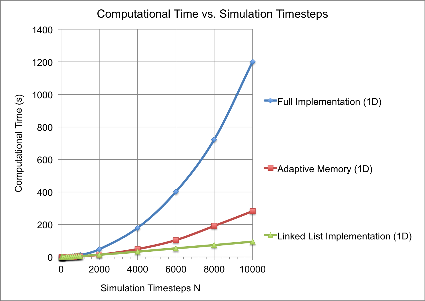
We verified our theoretical complexity results with simulated data. In Fig. 3.1 we show computation run times for simulations of various number of steps $N$ and demonstrate the complexity of the three numerical methods explored in this section (using one-dimensional versions for simplicity). For all algorithms we set $\gamma=0.8,\;D=1\frac{units^{2}}{s^{\gamma}},\;dt=0.1s,\;dx=0.6875\;units$ . We used adaptive step parameter $a$ and $\eta$ values of $20$ .

Trendlines were fit to the data using Matlab’s curve fitting toolbox. For the data corresponding to the full and adaptive memory implementations, the best fit lines were polynomials of second order (modeled with three coefficients). For the linked list implementation, the best fit trendline with minimum number of coefficients was a $Nlog_{2}N$ function.

•

full implementation simulation time = $p_{1}N^{2}+p_{2}N+p_{3}$ with $p_{1}=1.106e-5,\;p_{2}=5.5e-4,\;p_{3}=-0.0423$ and goodness of fit measure $R^{2}=0.9999$
•

adaptive memory simulation time = $p_{1}N^{2}+p_{2}N+p_{3}$ with $p_{1}=2.671e-5,\;p_{2}=1.441e-3,\;p_{3}=-0.05873$ and goodness of fit measure $R^{2}=0.9999$
•

linked list simulation time = $p_{1}Nlog_{2}\left(N\right)$ with $p_{1}=7.047e-4$ and goodness of fit measure $R^{2}=0.9992$ . This is the simplest trendline that was found to be a good fit. There were other functions that fit the data for the linked list implementation but required additional coefficients.

The data fitting and simulated data in Fig. 3.1 thus supports the theoretical analysis done in this section.

It is worth mentioning that there is additional overhead with the linked list implementation, involving the actual handling of the linked list (e.g. deleting and inserting new nodes, etc.). For this reason, for shorter simulations, the linked list algorithm may actually take longer to execute than the full or adaptive memory implementations. It is only when simulation length exceeds a certain point (and this threshold is determined by the details of the simulation, including parameter values) that the $NlogN$ time scaling complexity become more noticeable and the advantages of the linked list approach become more evident.

4 Error

In the last section we found that the algorithmic complexity for the linked list implementation is generally more computationally efficient than the full and adaptive memory implementations, with the exception of shorter simulation lengths where the overhead of dealing with linked list operations, may overwhelm the algorithmic scaling in time. However, with numerical algorithms, considerable advantages in one area usually come with some drawback or cost, in another. In this case, the accuracy of the linked list implementation is the drawback. In Fig. 4.1 we compare the error of the adaptive memory and linked list approaches, with the full implementation. We include both maximum error at each timepoint, and average error over the whole solution, at each timepoint. The reason we compare with the full implementation is because there is no closed form solution for the 2D fractional diffusion equation except for very specific circumstances, and these two algorithms were derived in part based on the basic finite difference scheme used in the full implementation. In Fig. 4.1 we see that the adaptive memory algorithm using the given parameters, converges over time, but the error with the linked list approach increases quickly and in an unbounded manner. There is some flexibility on setting parameters, and the larger $\eta$ is, the more accurate the simulation is, but the longer it takes (similar to the adaptive step parameter $a$ ). We leave as an open problem the analysis of the error resulting from the linked implementation, including whether it converges over time and its exact dependence on $\eta$ . Even in the case that error does not ever converge, one can set the value of $\eta$ depending on the required length of the simulation and how much error one is willing to tolerate during the simulation.

In Fig. 4.2 we also include a comparison of computational times for the simulations used in Fig. 4.1. It is clear that the adaptive memory and linked list approaches are much faster than the full implementation. However, the linked list simulation was not considerably faster than the adaptive step approach. If the simulation time was extended further, we would see this gap widen, however, as the $NlogN$ vs $N^{2}$ scaling effects came into play. Considering both Fig. 4.1 and 4.2, we may come to the conclusion that in many practical cases, the adaptive memory approach may provide the most reasonable trade-off between execution time and accuracy.

5 Conclusion

We have successfully characterized the stability of two finite difference algorithms used in solving the time-fractional diffusion equation. We provide our rationale for selecting a von Neumann analysis while also exploring a few alternative interpretations and approaches to analyzing stability. Using a von Neumann analysis we have developed bounding expressions for parameters like time step, spatial discretization, and grid size, that can be used to appropriately set parameters to ensure accurate simulations that reflect the true solution of the fractional diffusion equation. Our simulation results verify that our bounding expressions resulting from our stability analysis are valid and accurate. We also note here that the stability analysis of the linked list implementation should be explored, and we leave this as an open problem for further consideration.

We have also successfully characterized the algorithmic complexity of three finite difference algorithms introduced in [7]. We find that the full and adaptive step algorithms have a Big- $O$ complexity of $O\left(N^{2}\right)$ while the linked list scheme performs much better with $O\left(Nlog_{2}N\right)$ complexity. We compared our analytical results with simulated data and find they are in good agreement.

References

[1] Boris Baeumer, Subordinated advection-dispersion equation for contaminant transport, Water Resources …37 (2001), no. 6, 1543–1550.
[2] N Bhattacharya, Fractional Diffusion : Numerical Methods and Applications in Neuroscience, Ph.D. Dissertation in Bioengineering, UC San Diego (2014).
[3] ZEA Fellah, C Depollier, and M Fellah, Application of fractional calculus to the sound waves propagation in rigid porous materials: Validation via ultrasonic measurements, Acta Acustica united with …88 (2002), 34–39.
[4] Joseph E. Flaherty, Course notes - partial differential equations, University Lecture, http://www.cs.rpi.edu/ flaherje/.
[5] B. Henry, T. Langlands, and S. Wearne, Fractional cable models for spiny neuronal dendrites, Physical Review Letters 100 (2008), no. 12, 128103.
[6] Charles Hirsch, Numerical Computation of Internal and External Flows, Vol 1: Fundamentals of Numerical Discretization, vol. 1, John Wiley & Sons Ltd., 1988.
[7] Christopher L MacDonald, Nirupama Bhattacharya, Brian P Sprouse, and Gabriel A Silva, Efficient computation of the Grünwald-Letnikov fractional diffusion derivative using adaptive time step memory, Journal of Computational Physics (2015).
[8] Richard L Magin, Fractional Calculus in Bioengineering, Begell House Publishers, January 2006.
[9] R.L. Magin and M. Ovadia, Modeling the Cardiac Tissue Electrode Interface Using Fractional Calculus, Journal of Vibration and Control 14 (2008), no. 9-10, 1431–1442.
[10] B. Mathieu, P. Melchior, a. Oustaloup, and Ch. Ceyral, Fractional differentiation for edge detection, Signal Processing 83 (2003), no. 11, 2421–2432.
[11] Parviz Moin, Fundamentals of Engineering Numerical Analysis, Cambridge University Press, 2010.
[12] Keith B. Oldham and Jerome Spanier, The Fractional Calculus: Theory and Applications of Differentiation and Integration to Arbitrary Order, Dover Books on Mathematics, April 2006.
[13] I. Podlubny, Fractional Differential Equations, Academic Press New York, 1999.
[14] N. Sebaa, Z.E.a. Fellah, W. Lauriks, and C. Depollier, Application of fractional calculus to ultrasonic wave propagation in human cancellous bone, Signal Processing 86 (2006), no. 10, 2668–2677.
[15] Eugeniusz Soczkiewicz, Application of Fractional Calculus in the Theory of Viscoelasticity, Molecular and Quantum Acoustics 23 (2002), 397–404.
[16] SB Yuste and L. Acedo, On an explicit finite difference method for fractional diffusion equations, Arxiv preprint cs/0311011 (2003).