Experimental implementation of non-Clifford interleaved randomized benchmarking with a controlled-S gate
Abstract
Hardware efficient transpilation of quantum circuits to a quantum devices native gateset is essential for the execution of quantum algorithms on noisy quantum computers. Typical quantum devices utilize a gateset with a single two-qubit Clifford entangling gate per pair of coupled qubits, however, in some applications access to a non-Clifford two-qubit gate can result in more optimal circuit decompositions and also allows more flexibility in optimizing over noise. We demonstrate calibration of a low error non-Clifford Controlled- phase (CS) gate on a cloud based IBM Quantum computing using the Qiskit Pulse framework. To measure the gate error of the calibrated CS gate we perform non-Clifford CNOT-Dihedral interleaved randomized benchmarking. We are able to obtain a gate error of at a gate length 263 ns, which is close to the coherence limit of the associated qubits, and lower error than the backends standard calibrated CNOT gate.
I Introduction
Quantum computation holds great promise for speeding up certain classes of problems, however near-term applications are heavily restricted by the errors that occur on present day noisy quantum devices Preskill 2018. To run a computation on a quantum processor requires first calibrating a universal gate set – a small set of gates which can be used to implement an arbitrary quantum circuit – which has low error rates, and then transpiling the circuit to this set of gates. This transpilation should be done in a hardware-efficient manner to reduce the overall error by minimizing the use of the highest error gates Corcoles et al. 2020. Two of the most significant error sources on current devices are incoherent errors due to interactions with the environment, quantified by the coherence times of device qubits, and calibration errors in the gates used to implement a quantum computation Sheldon et al. 2016a; Wallman et al. 2015.
If a gate set could be perfectly calibrated the coherence time of the qubits would set the fundamental limit on error rates without active error correction. Thus the goal of gate calibration is to get as close to the coherence limit as possible. Current quantum hardware typically use a gate set consisting of arbitrary single-qubit rotations and a single entangling two-qubit gate McKay et al. 2018. State of the art single-qubit gate error rates in these systems approach McKay et al. 2017, where two-qubit gate errors are around Gambetta et al. 2017; Xu et al. 2020; Foxen et al. 2020, see also Appendix A. In superconducting qubit systems using fixed-frequency transmon qubits a microwave-only two-qubit entangling gate may be implemented using the cross-resonance (CR) interaction Chow et al. 2011. The CR interaction can be used to implement a high fidelity Controlled-NOT (CNOT) gate Sheldon et al. 2016b. Gate sets with a Clifford two-qubit like CNOT are appealing as a variety of averaged errors in a Clifford gateset can be can be robustly measured using various randomized benchmarking (RB) protocols Magesan et al. 2011; Magesan et al. 2012; Wood and Gambetta 2018; McKay et al. 2016; Wallman et al. 2015; McKay et al. 2020.
In some cases it may be favorable to introduce an additional two-qubit gate to a gate set if it enables more hardware efficient compilation of relevant circuits, however this adds the overhead of additional calibration and characterization of the gate errors. One such gate is the Controlled-Phase (CS) gate, which is a non-Clifford two-qubit entangling gate that is universal when combined with the Clifford group Cross et al. 2016. The CS gate is particularly attractive to fixed-frequency transmon qubit systems as it can be implemented using the CR interaction, since it is locally equivalent to . This means it can be calibrated using the same techniques as the CNOT gate, but with a shorter gate duration or lower power, potentially leading to a higher fidelity two-qubit gate when calibrated close to the coherence limit. Furthermore the CS gate is a member the CNOT-Dihedral group and can be benchmarked using CNOT-Dihedral randomized benchmarking Cross et al. 2016. Recently an optimal decomposition algorithm for two-qubit circuits into the Clifford + CS gates was developed Glaudell et al. 2020. This method minimizes the number of non-Clifford (CS) gates, which is important in the context of quantum error correction as non-Clifford gates require additional resources such as magic-state distillation to prepare fault-tolerantly Bravyi and Kitaev 2005. However, in non-fault tolerant near term devices it is often preferable to minimize the total number of two-qubit gates in a decomposition rather than non-Clifford gates. An optimal decomposition for gates generated by the CNOT-Dihedral in terms of the number of CNOT and CS gates has also recently been developed Garion and Cross 2020. Another example is the Toffoli gate which can be decomposed into 6 CNOT gates and single qubit gates, but requires only 5 two-qubit gates in its decomposition if the CS and gates are also available Barenco et al. 1995.
In this work we calibrate CS and gates of varying durations on an IBM Quantum system and benchmark the gate error rates by performing the first experimental demonstration of interleaved CNOT-Dihedral randomized benchmarking. For specific gate durations we are able to obtain a high-fidelity CS gate approaching the coherence limit, which due to the shorter CR interaction time results in a lower error rate than can be obtained for a CNOT gate. In addition to RB we also compute the average gate error of the CS gate using two-qubit quantum process tomography (QPT) and compare to the values obtained from RB. Pulse-level calibration was done using Qiskit Pulse Alexander et al. 2020, and the RB and QPT experiments were implemented using the open source Qiskit computing software stack Abraham and et al 2019 through the IBM Quantum cloud provider.
II CNOT-Dihedral Randomized Benchmarking
We describe the protocol for estimating the average gate error of the CS gate using interleaved CNOT-Dihedral Randomized Benchmarking, which is a natural generalization of the CNOT-Dihedral RB procedure described in Cross et al. 2016 with interleaved RB Magesan et al. 2012 to estimate individual gate fidelities for the CS gate
In the following we let denote the CNOT-Dihedral group on qubits and denote a unitary element of . Here the CNOT-Dihedral group is generated by the single-qubit gates and the CNOT gate. More precisely,
where . We denote , , , as the single-qubit Pauli matrices and .
Step 1: Standard CNOT-Dihedral benchmarking.
Randomly sample elements uniformly from , and compute the ()th element from the inverse of their composition, . Denote by the -tuple . For each sequence, we prepare an input state , and apply the composition of the gates that ideally would be
and then measure the expectation value of an observable .
Assuming each gate has an associated error , the sequence is implemented as
| (1) |
The expectation value of is . Averaging this overlap over independent sequences of length gives an estimate of the average sequence fidelity
| (2) |
where is the average quantum channel.
We decompose the input state and this final measurement operator in the Pauli basis (an orthonormal basis of the -qubit Hermitian operators space, constructed of single-qubit Pauli matrices). This gives and . Given that the gate errors are close to the average of all errors Cross et al. 2016, the average sequence fidelity is
where and , with being tensor products of and gates.
Each of the two exponential decays and can be observed by choosing appropriate input states. For example, if we choose the input state then where . On the other hand, if we choose then where , with tensor products of and gates.
The channel parameters and can be extracted by fitting the average sequence fidelity to an exponential. From the average depolarizing channel parameter for a group element is given by
| (3) |
and the corresponding average gate error is given by
| (4) |
Step 2: Interleaved CNOT-Dihedral sequences.
Choose a sequence of unitary gates where the first element is chosen uniformly at random from , the second is always chosen to be , and alternate between uniformly random elements from and fixed up to the -th random gate. The element is chosen to be the inverse of the composition of the first random gates and interlaced gates, . We adopt the convention of defining the length of a sequence by the number of random gates .
For each sequence, we prepare an input state , apply
and measure an operator .
Assuming that the gate has an associated error and that each gate has an associated error , the sequence is implemented as
| (5) |
The overlap with is . Averaging this overlap over independent sequences of length gives an estimate of the new sequence fidelity
where is the average quantum channel.
Similarly to Step 1, we fit and obtain the depolarizing parameter , according to Eq. (3). Using the values obtained for and , the gate error of , which is given by
| (6) |
and must lie in the range , where can be estimated using Magesan et al. 2012 Eq. (5), or Kimmel et al. 2014 Eq. (VI.1). Note that one has to be careful in interpreting the results of an interleaved experiment, as in some cases might be large compared to .
III Implementing the Controlled-S gate
We calibrate CS gates of varying gate durations using Qiskit Pulse and measure the average gate error using the interleaved CNOT-Dihedral RB protocol in II. We use the CR pulse sequence as a generator of two-qubit entanglement Rigetti and Devoret 2010; Chow et al. 2011. The CR pulse is realized by irradiating one (control) qubit with a microwave pulse at the transition frequency of another (target) qubit. The stimulus drives the quantum state of the target qubit with the direction of rotation depending on the quantum state of the control qubit. This controlled rotation is used to create two-qubit entangling gates such as CNOT and CS.
The two-qubit system driven by the CR pulse with amplitude and phase can be approximated by an effective block-diagonal time-independent Hamiltonian Magesan and Gambetta 2020; Malekakhlagh et al. 2020
| (7) | ||||
where the qubit ordering is control target, and and represent the interaction strength of the corresponding Pauli Hamiltonian terms. In the absence of noise, the ideal CR evolution for a constant-amplitude pulse is written as an unitary operator
| (8) |
where is the length of the CR pulse. We also define the unitary operator created by an arbitrary two-qubit generator as
| (9) |
where , are arbitrary single qubit operators, and we use .
As can be seen by examining Eq. (7), the CR pulse induces three entangling interaction terms (, , and ), in addition to potentially many unwanted local rotations with different amplitudes. By appropriately calibrating the phase of the CR drive , the term is the dominant term among the interactions and is the key term for executing two-qubit gates in this system. As with the standard CNOT gate, we can compose a CS gate by isolating the ZX interaction with a refocusing sequence and single qubit pre- and post-rotations:
| (10) |
where is the Hadamard operator. As shown in Eq. (10), we need to develop the calibration procedure to find an amplitude and a phase where and the other terms become zero. The CR Hamiltonian includes a large term as a result of the off-resonant driving of the control qubit; , and can also be large for transmon qubits Magesan and Gambetta 2020. However, the strengths of and terms are expected to be negligibly weak in our device. We note that both and terms commute with the term of interest, while and terms anti-commute with the inversion of the control qubit . In addition, the term is the even function and both and terms are odd functions of the drive amplitude . Accordingly, we can effectively eliminate the impact of those unwanted terms with the two-pulse echoed CR sequence Córcoles et al. 2013 expressed as
| (11) |
This sequence consists of two CR pulses with opposite drive amplitude, each one followed by a -rotation refocus pulse on the control qubit. Here we also assume the negligible impact of the term which is generally introduced by the physical crosstalk between the control and the target qubit Sheldon et al. 2016b.
III.1 Gate Calibration and Benchmarks
To experimentally implement the CS and gates we use the 27 qubit IBM Quantum system ibmq_paris with fixed-frequency and dispersively coupled transmon qubits. Qubit 0 and the qubit 1 of this system are assigned as the control and the target qubit, respectively. The resonance frequency and anharmonicity of the control (target) qubit are 5.072 (5.020) GHz and -336.0 (-321.0) MHz.
The pulses realized in practice are not constant-amplitude pulses, rather the amplitude is increased and decreased smoothly. We implement the CR pulse as a flat top Gaussian, with flat-top length , and Gaussian rising and falling edges each with length (). We use a constant Gaussian edge with ns with ns standard deviation and vary the length of the duration of the square flat-top pulse . The minimum pulse duration is ns, yielding a pure Gaussian shape. The overhead of single-qubit gates in the echoed CS sequence in Eq. (10) for the ibmq_paris backend is 106.7 ns, giving a total echoed CS gate time of . The single-qubit gates are optimized by merging consecutive rotations using the Qiskit circuit transpiler with optimization_level = 1 followed by conversion to a pulse schedule Alexander et al. 2020.
We performed calibration to a CR rotation angle for different values of . This was done by first performing a rough calibration of by scanning those parameters, followed by the closed-loop fine calibration with standard error amplification sequences (see Appendix C for details). The calibrated pulse schedule of the CS gate with ns ( ns) is shown in Fig. 1(a).

The average gate error of the calibrated CS gate is evaluated by using the interleaved CNOT-Dihedral RB with 10 sequence lengths , and 10 samples for each . Each experiment is executed 1024 times for both input states and both with and without interleaving the CS gate. An example of measured RB decay curves for = 21.3 ns are shown in Fig. 1(b). The exponential fit of the decay curves yields and , giving an estimated average gate error of the CS gate of . In addition to RB we also perform quantum process tomography (QPT) Mohseni et al. 2008 and compute the average gate fidelity from the reconstructed process, see the Appendix B for the details. The average gate error calculated from the tomographic fit for ns was which is slightly higher but still comparable to the value estimated from the interleaved CNOT-Dihedral RB experiment.
III.2 Gate Duration Dependence

We perform the same calibration and benchmarking procedures for different flat-top width from 0 ns to 355.6 ns ( from 219.3 ns to 930.5 ns) and measure the average gate errors by both the interleaved CNOT-Dihedral RB experiment and QPT. In this experiment, we use a reduced set of RB sequence lengths to reduce the total number of experiments while keeping the accuracy of the estimated gate error high.
We measure the qubit coherence times and with relaxation and Hahn echo sequences Bylander et al. 2011, respectively, to monitor the stability of physical properties of qubits. These experiments are inserted immediately before each calibration experiment and yield coherence times of ()s and ()s for the control (target) qubit during the experiment. Here, the error bars correspond to the standard deviation over the duration of the whole set of calibration and benchmarking experiments. A lower bound of gate error at is calculated based on the measured and values with the total gate duration , see Appendix G of Ref. Sundaresan et al. 2020. The coherence_limit function in Qiskit Ignis IBM 2019 is used for the calculation, presented in Fig. 2. The device was accessed via the cloud through a fair-share queuing model used in IBM Quantum systems. The time in between experiments was about 168 minutes on average, thus the experiment could be subject to some parameter fluctuations due to noise with a long characteristic time Schlör et al. 2019.
Nevertheless, as in Fig. 2 shows, our calibration method provides highly accurate results and allows to approach the coherence limit for appropriately chosen gate times. This dependence on agrees well with the slope predicted by the coherence limit for ns. We also plot as a reference since QPT is conventionally used to evaluate the performance of non-Clifford gates. These lines show reasonable agreement though tends to show slightly higher gate errors than . This is expected as QPT is sensitive to state preparation and measurement errors, though measurement errors have been reduced by using readout error mitigation. The interleaved CNOT-Dihedral RB experiment requires only 24 circuit executions per single error measurement, while the two-qubit QPT requires 148 circuit executions with the readout error mitigation. The smaller experimental cost to measure enables us to average the result over 10 different random circuits, which is empirically sufficient to obtain a reproducible outcome, at a practical queuing time with ibmq_paris. The nearly stable offset of from the coherence limit possibly indicates the presence of coherent errors due to imperfection of calibration.
In the region ns, both gate errors show a significant increase from the coherence limit. In this regime the drive amplitude of the CR pulse rapidly increases in order to guarantee that the total accumulated rotation angle is for shorter . The amplitude of crosstalk measured at ns is 176.2 kHz, while one at ns is 19.4 kHz. Although the term is refocused and has negligible contribution, the remained term can still impact on the measured gate errors. Thus, at we calibrate a CS gate with a compensation tone on the target qubit to suppress the physical crosstalk between qubits (see Appendix D for details). The calibrated pulse sequences with and without the compensation tone yield of and , respectively. These comparable results indicate the physical crosstalk is relatively suppressed in this quantum device and other noise sources are dominant for ns. For example, at high power the perturbation theory used to obtain the average CR Hamiltonian may break down, and hence also calibration scheme based on this decomposition.
The reasons for imperfection of two-qubit gates in superconducting qubits have been investigated and associated with various mechanisms such as nonideal signal generation, residual coupling, CR-induced interaction Ganzhorn et al. 2020; Noguchi et al. 2020; Ku et al. 2020, and leakage to the higher energy levels McKay et al. 2016; Rol et al. 2019. Although a further analysis of the error mechanisms in this regime of high-power pulses is beyond the scope of this study, initial results indicate that coherent population transfer out of the two-qubit manifold into the higher levels, and interaction terms, are not the relevant mechanisms Kanazawa. At the same time, the coherence limit can be further lowered by reducing the time spent on single-qubit gates. At ns with the minimum of , the refocusing pulse and local rotations occupy 40% of the total gate time , yielding a non-negligible impact on the gate error.
The interleaved CNOT-Dihedral Randomized Benchmarking technique can be used to evaluate any quantum gate in the CNOT-Dihedral group regardless of its physical qubit implementation. The calibration protocol is also general to devices which are capable of driving the CR interaction.
IV Conclusion
We have demonstrated calibration of a high fidelity non-Clifford CS gate on 27 qubit IBM Quantum system ibmq_paris. This gate is not currently included in the standard basis gates of IBM Quantum systems, and it was calibrated and benchmarked entirely using open source software available in Qiskit. Since the CS gate is non-Clifford, robust characterization of the average gate error cannot be done using standard RB. To benchmark performance of the non-Clifford gate we performed the first experimental demonstration of two-qubit interleaved CNOT-Dihedral RB, which allow efficient and robust characterization of a universal gateset containing the CS gate.
We obtained a minimal gate error of with appropriately shaped echoes and a total gate time of ns. The gate error reported for the standard two-qubit CNOT gate provided by ibmq_paris is . Thus the presented CS gate error is comparable with half the CNOT error. By performing RB and QPT for a variety of gate lengths we were also able to study the performance of the CS gate in different regimes and observed a break down in performance if gate lengths were reduced below the best value obtained for ns. This is consistent with previous literature on CNOT calibration using the cross-resonance interaction in the high power regime.
The expansion of the native two-qubit gateset of a Cloud quantum device with additional low error calibrated gates allows for improved hardware efficient transpilation of quantum circuits. This is important for executing quantum algorithms on noisy quantum devices without error correction, and for reducing the error correction overhead when fault-tolerant devices with active error correction are available.
Acknowledgements
We thank Ken Xuan Wei for discussion about the CS gate calibration and providing us with the pulse sequence to investigate local coherent errors. DCM and SS acknowledge partial support from the ARO under Contract No. W911NF-14-1-0124.
References
- Preskill (2018) John Preskill, “Quantum computing in the nisq era and beyond,” Quantum 2, 79 (2018).
- Corcoles et al. (2020) Antonio D. Corcoles, Abhinav Kandala, Ali Javadi-Abhari, Douglas T. McClure, Andrew W. Cross, Kristan Temme, Paul D. Nation, Matthias Steffen, and Jay M. Gambetta, “Challenges and opportunities of near-term quantum computing systems,” Proceedings of the IEEE 108, 1338–1352 (2020).
- Sheldon et al. (2016a) Sarah Sheldon, Lev S. Bishop, Easwar Magesan, Stefan Filipp, Jerry M. Chow, and Jay M. Gambetta, “Characterizing errors on qubit operations via iterative randomized benchmarking,” Phys. Rev. A 93, 012301 (2016a).
- Wallman et al. (2015) Joel Wallman, Chris Granade, Robin Harper, and Steven T Flammia, “Estimating the coherence of noise,” New J. Phys. 17, 113020 (2015).
- McKay et al. (2018) David C. McKay, Thomas Alexander, Luciano Bello, Michael J. Biercuk, Lev Bishop, Jiayin Chen, Jerry M. Chow, Antonio D. Córcoles, Daniel J. Egger, Stefan Filipp, Juan Gomez, Michael Hush, Ali Javadi-Abhari, Diego Moreda, Paul Nation, Brent Paulovicks, Erick Winston, Christopher J. Wood, James Wootton, and Jay M. Gambetta, “Qiskit backend specifications for OpenQASM and OpenPulse experiments,” (2018), arXiv:1809.03452 [quant-ph] .
- McKay et al. (2017) David C. McKay, Christopher J. Wood, Sarah Sheldon, Jerry M. Chow, and Jay M. Gambetta, “Efficient gates for quantum computing,” Phys. Rev. A 96, 022330 (2017).
- Gambetta et al. (2017) Jay M. Gambetta, Jerry M. Chow, and Matthias Steffen, “Building logical qubits in a superconducting quantum computing system,” npj Quantum Information 3 (2017).
- Xu et al. (2020) Yuan Xu, Ji Chu, Jiahao Yuan, Jiawei Qiu, Yuxuan Zhou, Libo Zhang, Xinsheng Tan, Yang Yu, Song Liu, Jian Li, Fei Yan, and Dapeng Yu, “High-fidelity, high-scalability two-qubit gate scheme for superconducting qubits,” Phys. Rev. Lett. 125, 240503 (2020).
- Foxen et al. (2020) B. Foxen, C. Neill, A. Dunsworth, P. Roushan, B. Chiaro, A. Megrant, J. Kelly, Zijun Chen, K. Satzinger, R. Barends, F. Arute, K. Arya, R. Babbush, D. Bacon, J. C. Bardin, S. Boixo, D. Buell, B. Burkett, Yu Chen, R. Collins, E. Farhi, A. Fowler, C. Gidney, M. Giustina, R. Graff, M. Harrigan, T. Huang, S. V. Isakov, E. Jeffrey, Z. Jiang, D. Kafri, K. Kechedzhi, P. Klimov, A. Korotkov, F. Kostritsa, D. Landhuis, E. Lucero, J. McClean, M. McEwen, X. Mi, M. Mohseni, J. Y. Mutus, O. Naaman, M. Neeley, M. Niu, A. Petukhov, C. Quintana, N. Rubin, D. Sank, V. Smelyanskiy, A. Vainsencher, T. C. White, Z. Yao, P. Yeh, A. Zalcman, H. Neven, and J. M. Martinis (Google AI Quantum), “Demonstrating a continuous set of two-qubit gates for near-term quantum algorithms,” Phys. Rev. Lett. 125, 120504 (2020).
- Chow et al. (2011) Jerry M. Chow, A. D. Córcoles, Jay M. Gambetta, Chad Rigetti, B. R. Johnson, John A. Smolin, J. R. Rozen, George A. Keefe, Mary B. Rothwell, Mark B. Ketchen, and M. Steffen, “Simple all-microwave entangling gate for fixed-frequency superconducting qubits,” Phys. Rev. Lett. 107, 080502 (2011).
- Sheldon et al. (2016b) Sarah Sheldon, Easwar Magesan, Jerry M. Chow, and Jay M. Gambetta, “Procedure for systematically tuning up cross-talk in the cross-resonance gate,” Phys. Rev. A 93, 060302 (2016b).
- Magesan et al. (2011) Easwar Magesan, J. M. Gambetta, and Joseph Emerson, “Scalable and robust randomized benchmarking of quantum processes,” Phys. Rev. Lett. 106, 180504 (2011).
- Magesan et al. (2012) Easwar Magesan, Jay M. Gambetta, B. R. Johnson, Colm A. Ryan, Jerry M. Chow, Seth T. Merkel, Marcus P. da Silva, George A. Keefe, Mary B. Rothwell, Thomas A. Ohki, Mark B. Ketchen, and M. Steffen, “Efficient measurement of quantum gate error by interleaved randomized benchmarking,” Phys. Rev. Lett. 109, 080505 (2012).
- Wood and Gambetta (2018) Christopher J. Wood and Jay M. Gambetta, “Quantification and characterization of leakage errors,” Phys. Rev. A 97, 032306 (2018).
- McKay et al. (2016) David C. McKay, Stefan Filipp, Antonio Mezzacapo, Easwar Magesan, Jerry M. Chow, and Jay M. Gambetta, “Universal gate for fixed-frequency qubits via a tunable bus,” Phys. Rev. Applied 6 (2016).
- McKay et al. (2020) David C McKay, Andrew W Cross, Christopher J Wood, and Jay M Gambetta, “Correlated randomized benchmarking,” arXiv preprint arXiv:2003.02354 (2020).
- Cross et al. (2016) Andrew W Cross, Easwar Magesan, Lev S Bishop, John A Smolin, and Jay M Gambetta, “Scalable randomised benchmarking of non-clifford gates,” npj Quantum Information 2 (2016).
- Glaudell et al. (2020) Andrew N. Glaudell, Neil J. Ross, and Jacob M. Taylor, “Optimal two-qubit circuits for universal fault-tolerant quantum computation,” (2020), arXiv:2001.05997 [quant-ph] .
- Bravyi and Kitaev (2005) Sergey Bravyi and Alexei Kitaev, “Universal quantum computation with ideal clifford gates and noisy ancillas,” Phys. Rev. A 71 (2005).
- Garion and Cross (2020) Shelly Garion and Andrew W. Cross, “Synthesis of CNOT-Dihedral circuits with optimal number of two qubit gates,” Quantum 4, 369 (2020).
- Barenco et al. (1995) Adriano Barenco, Charles H. Bennett, Richard Cleve, David P. DiVincenzo, Norman Margolus, Peter Shor, Tycho Sleator, John A. Smolin, and Harald Weinfurter, “Elementary gates for quantum computation,” Phys. Rev. A 52, 3457–3467 (1995).
- Alexander et al. (2020) Thomas Alexander, Naoki Kanazawa, Daniel J Egger, Lauren Capelluto, Christopher J Wood, Ali Javadi-Abhari, and David C McKay, “Qiskit pulse: programming quantum computers through the cloud with pulses,” Quantum Science and Technology 5, 044006 (2020).
- Abraham and et al (2019) Héctor Abraham and et al, “Qiskit: An open-source framework for quantum computing,” (2019).
- Kimmel et al. (2014) Shelby Kimmel, Marcus P. da Silva, Colm A. Ryan, Blake R. Johnson, and Thomas Ohki, “Robust extraction of tomographic information via randomized benchmarking,” Phys. Rev. X 4 (2014).
- Rigetti and Devoret (2010) Chad Rigetti and Michel Devoret, “Fully microwave-tunable universal gates in superconducting qubits with linear couplings and fixed transition frequencies,” Phys. Rev. B 81, 134507 (2010).
- Magesan and Gambetta (2020) Easwar Magesan and Jay M. Gambetta, “Effective hamiltonian models of the cross-resonance gate,” Phys. Rev. A 101, 052308 (2020).
- Malekakhlagh et al. (2020) Moein Malekakhlagh, Easwar Magesan, and David C. McKay, “First-principles analysis of cross-resonance gate operation,” Phys. Rev. A 102, 042605 (2020).
- Córcoles et al. (2013) A. D. Córcoles, Jay M. Gambetta, Jerry M. Chow, John A. Smolin, Matthew Ware, Joel Strand, B. L. T. Plourde, and M. Steffen, “Process verification of two-qubit quantum gates by randomized benchmarking,” Phys. Rev. A 87, 030301 (2013).
- Mohseni et al. (2008) M. Mohseni, A. T. Rezakhani, and D. A. Lidar, “Quantum-process tomography: Resource analysis of different strategies,” Phys. Rev. A 77, 032322 (2008).
- Bylander et al. (2011) Jonas Bylander, Simon Gustavsson, Fei Yan, Fumiki Yoshihara, Khalil Harrabi, George Fitch, David G. Cory, Yasunobu Nakamura, Jaw-Shen Tsai, and William D. Oliver, “Noise spectroscopy through dynamical decoupling with a superconducting flux qubit,” Nature Physics 7, 565–570 (2011).
- Sundaresan et al. (2020) Neereja Sundaresan, Isaac Lauer, Emily Pritchett, Easwar Magesan, Petar Jurcevic, and Jay M. Gambetta, “Reducing unitary and spectator errors in cross resonance with optimized rotary echoes,” PRX Quantum 1, 020318 (2020).
- IBM (2019) IBM, “Qiskit Ignis,” https://github.com/Qiskit/qiskit-ignis (2019), version 0.3.
- Schlör et al. (2019) Steffen Schlör, Jürgen Lisenfeld, Clemens Müller, Alexander Bilmes, Andre Schneider, David P. Pappas, Alexey V. Ustinov, and Martin Weides, “Correlating decoherence in transmon qubits: Low frequency noise by single fluctuators,” Phys. Rev. Lett. 123, 190502 (2019).
- Ganzhorn et al. (2020) M. Ganzhorn, G. Salis, D. J. Egger, A. Fuhrer, M. Mergenthaler, C. Müller, P. Müller, S. Paredes, M. Pechal, M. Werninghaus, and S. Filipp, “Benchmarking the noise sensitivity of different parametric two-qubit gates in a single superconducting quantum computing platform,” Phys. Rev. Research 2, 033447 (2020).
- Noguchi et al. (2020) Atsushi Noguchi, Alto Osada, Shumpei Masuda, Shingo Kono, Kentaro Heya, Samuel Piotr Wolski, Hiroki Takahashi, Takanori Sugiyama, Dany Lachance-Quirion, and Yasunobu Nakamura, “Fast parametric two-qubit gates with suppressed residual interaction using the second-order nonlinearity of a cubic transmon,” Phys. Rev. A 102, 062408 (2020).
- Ku et al. (2020) Jaseung Ku, Xuexin Xu, Markus Brink, David C. McKay, Jared B. Hertzberg, Mohammad H. Ansari, and B. L. T. Plourde, “Suppression of unwanted interactions in a hybrid two-qubit system,” Phys. Rev. Lett. 125, 200504 (2020).
- Rol et al. (2019) M. A. Rol, F. Battistel, F. K. Malinowski, C. C. Bultink, B. M. Tarasinski, R. Vollmer, N. Haider, N. Muthusubramanian, A. Bruno, B. M. Terhal, and L. DiCarlo, “Fast, high-fidelity conditional-phase gate exploiting leakage interference in weakly anharmonic superconducting qubits,” Phys. Rev. Lett. 123, 120502 (2019).
- (38) N. Kanazawa, unpublished.
- Bravyi et al. (2020) Sergey Bravyi, Sarah Sheldon, Abhinav Kandala, David C. Mckay, and Jay M. Gambetta, “Mitigating measurement errors in multi-qubit experiments,” (2020), arXiv:2006.14044 [quant-ph] .
- Krinner et al. (2019) S. Krinner, S. Storz, P. Kurpiers, P. Magnard, J. Heinsoo, R. Keller, J. Lütolf, C. Eichler, and A. Wallraff, “Engineering cryogenic setups for 100-qubit scale superconducting circuit systems,” EPJ Quantum Technology 6, 2 (2019).
- Ali Ahmed et al. (2013) Mustafa Ahmed Ali Ahmed, Gonzalo A. Álvarez, and Dieter Suter, “Robustness of dynamical decoupling sequences,” Phys. Rev. A 87, 042309 (2013).
Appendix A Basis Gate Information
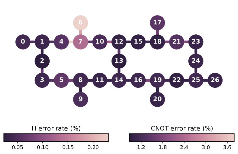
In this paper all experiments are performed via cloud access to IBM Quantum system ibmq_paris. The backend provider calibrates single-qubit and two-qubit basis gates on a regular basis and provides pulse schedules and gate errors to users. The gate error distribution at the time of experiment (2020-05-20 05:48 UTC) is shown in Fig. 3. The averaged single-qubit gate error is , while that of two-qubit gates is . The single-qubit gate error of the qubit 0 and 1, which are use in the CS gate, are and , respectively. The two-qubit CNOT gate error between these qubits is .
Appendix B Quantum process tomography
QPT was done using convex maximum likelihood estimation fitter with completely positive and trace-preserving (CPTP) constraints from the tomography module of Qiskit Ignis. The preparation basis and measurement basis was used for each qubit. We performed repetitions (shots) for each QPT basis configuration and readout error calibration circuit. This requires 148 different experimental circuit executions per single evaluation. The readout error calibration circuit data was used to construct a 2-qubit measurement assignment matrix characterizing the Z-basis classical readout errors Bravyi et al. 2020. This was used to compute noisy measurement basis POVM elements in the QPT fitter objective function to apply readout error mitigation during the QPT fit. Note that this only mitigates the readout errors from the final Z-basis measurement. Measurement errors arising from gate errors in the gates to change tomography measurement bases will not be affected.
The interval of each experiment trigger in this device is set to 1000 s, therefore the minimum execution time of the whole experiment is estimated to be about 2.5 minutes.
Appendix C Calibrating CS Gate

The single qubit gates used for the echo sequence and local rotations are provided by ibmq_paris. We calibrate the CR pulse amplitude and its phase by the rough parameter scan followed by the closed-loop calibration. These parameters are determined based on the two-pulse echoed CR sequence shown in Eq. (11). This approach simplifies the calibration, namely, we don’t need to take non-negligible and terms into account when we fit the experimental results for calibration parameters. Calibrated sequence is used to realize the CS with local rotations shown in Eq. (10).
C.1 Rough Parameter Scan
We initialized both qubits in the ground state and perform a rough scan of the CR pulse amplitude with the pulse schedule:
The schedule is followed by the measurement of the target qubit in the -basis. The sinusoidal fit for the measured population of the target qubit with with different gives an estimate of the CR amplitude where the angle of controlled rotation is approximately . A typical experimental result for ns is shown in Fig. 4(a).
By using this , we scan the CR phase with two pulse schedules and :
The schedule () drives the echo sequence twice with the control qubit of the ground (excited) state. Note that the last two operations correspond to the projection into -basis for the following measurement. The flip of the state of the control qubit leads the controlled rotation of the target qubit state with opposite direction as illustrated in Fig. 4(b). This opposite rotation of around an azimuthal angle of the target qubit Bloch sphere yields measured outcome of 1 for and , respectively, at the optimal phase where . Here is the phase offset from the unknown transfer function of the coaxial cable assembly Krinner et al. 2019. The phase gives a rough estimate of the CR phase where the term of interest is maximized while the unwanted term is eliminated.
C.2 Closed-loop Fine Calibration
We use the roughly estimated parameters as an initial guess of closed-loop calibrations. We first optimize the CR pulse amplitude with following experiment:
where is number of repeated sequences. This schedule prepares the target qubit in the superposition state and repeat the echo sequence times to apply a controlled rotation of . Because the initial guess of is estimated by the parameter scan in the coarse precision with a finite error , repeating for different can accumulate and this error appears as over rotation from the superposition state, as shown in Fig. 4(c). The fit for the over rotation as a function of yields precise estimate of , and we iteratively update the initial guess to optimize the CR pulse amplitude to where . Here we use and repeat updating the CR amplitude until the over rotation error reaches below the threshold value of rad.
With the optimized amplitude , we tune the CR phase with following experiment:
This sequence also accumulates the small phase error as function of . We iteratively update the CR phase until the same threshold value with the amplitude calibration to obtain the optimal phase where .
Appendix D Crosstalk Estimation
The unwanted local rotation terms and can be simultaneously amplified with the following sequence combined with the XY-4 dynamical decoupling Ali Ahmed et al. 2013 on the control qubit:
where . Here, the CR pulse with the same sign is repeatedly applied while changing the state of control qubit. This pulse sequence refocuses (and hence eliminates) controlled rotation terms such as and , allowing us to precisely estimate the strength of weak local rotation terms , amplified in the absence of strong two-qubit interactions.
This technique can be used to calibrate a compensation tone that eliminates the term caused by the physical crosstalk between qubits Sheldon et al. 2016b. The compensation tone is applied to the drive channel of the target qubit d1, in parallel with . This single-qubit pulse is shaped as a flat-top pulse with Gaussian edges of identical duration as the pulse, with its own calibrated amplitude and phase . First, we repeat for without the compensation tone and measure the Pauli expectation value of the target qubit. The fit for the oscillation over the total CR gate time yields the strength of the total unwanted local rotation terms. At ns, the unwanted local rotation strength of 176.2 kHz was observed. This strength was reduced to 6.7 kHz with the calibrated compensation tone with and rad. The experimental result is shown in Fig. 4(d).