openDD: A Large-Scale Roundabout Drone Dataset
Abstract
Analyzing and predicting the traffic scene around the ego vehicle has been one of the key challenges in autonomous driving. Datasets including the trajectories of all road users present in a scene, as well as the underlying road topology are invaluable to analyze the behavior of the various traffic participants. The interaction between the traffic participants is especially high in intersection types that are not regulated by traffic lights, the most common one being the roundabout. We introduce the openDD dataset, including 84,774 accurately-tracked trajectories and HD map data of seven different roundabouts. The openDD dataset is annotated using images taken by a drone in 501 separate flights, totalling in over 62 hours of trajectory data. As of today the openDD is by far the largest publicly available trajectory dataset recorded from a drone perspective, while comparable datasets span 17 hours at most. The data is available, for both commercial and non-commercial use, at: http://www.l3pilot.eu/openDD.
I INTRODUCTION
In recent years autonomous driving has become one of the major applications for numerous fields of research. A main challenge faced in autonomous driving is the prediction of the traffic scene surrounding the ego vehicle. Predicting the surrounding traffic scene is particularly difficult in urban and rural scenarios due to the high inter-dependency between the involved road users. One way to face this challenge is to use increasing amounts of data, causing a surge of popularity of data-driven approaches that rely on large-scale datasets in recent years [1, 2, 3, 4]. Other applications of trajectory datasets include the modeling and analysis of driving behavior [5] and the analysis of safety of the autonomous driving function [6].

Datasets recorded from a ground view instead of a bird’s eye perspective are limited by occlusions and the restricted field of view of the recording device at the ground. Labeling the trajectories with the help of image data captured by an aerial drone ensures a complete overview of the traffic situation and enables algorithms that use the dataset to take all present road users into account. The interaction between different road users is particularly high in intersections that are not regulated by traffic lights, the most common being the roundabout. In the openDD dataset presented in this work, seven roundabouts with different topologies are covered, one of them shown in Fig. 1. The dataset includes trajectories of all recorded road users, shapefiles and an extensible markup language (XML)file, describing the road topology of the underlying intersections. One reference image taken by the drone is provided per intersection. An exemplary visualization of the data included in the dataset can be seen in Fig. 1. As shown there, all dynamic traffic participants are accurately tracked in the relevant area surrounding the roundabout, and also vehicles hard to see for the human eye, such as the grey car on top of the picture are accurately detected. The introduced openDD dataset spans more than hours in total, covers trajectories, and can be accessed on the following website: http://www.l3pilot.eu/openDD.
II RELATED WORK
| Dataset Name | Length | Situations | # locations | # trajectories | Map | Classes | License |
| Stanford | campus | 10,240 | none | pedestrians, bicycles, cars, | non-commercial | ||
| Drone [7] | skateboards, carts, buses | ||||||
| highD [8] | highway | 6 | 110,000 | none | cars, trucks | non-commercial | |
| CITR [9] | parking lot | 1 | 340 | none | pedestrians | non-commercial | |
| DUT [9] | urban intersections, | 2 | 1,793 | none | pedestrians | non-commercial | |
| shared space | |||||||
| inD [10] | urban intersections | 4 | 11,500 | none | pedestrians, bicycles, cars, | non-commerical | |
| trucks, buses | |||||||
| INTERACTION | urban intersections, | 11 | 40,054 | lanelet2 | cars, pedestrians | non-commerical | |
| [11] | highway | [12] | |||||
| openDD | roundabouts | 7 | 84,774 | shapefiles | cars, vans, trucks, buses, | non-commerical | |
| pedestrians, trailers, | & commercial | ||||||
| motorcycles, bicyclists |
Table Igives an overview of trajectory datasets recorded from a drone perspective and their characteristics.
The Stanford drone dataset [7] was the first publicly available trajectory dataset recorded from a drone’s perspective and is tailored to the analysis of pedestrian trajectories. It consists of hours of data over eight unique locations on the campus and has a high percentage rate of labeled pedestrians and cyclists, while only about of the labeled targets are cars. The DUT and CITR datasets [9] are especially designed for the analysis of the behavior of pedestrians when interacting with vehicles and span less than half an hour in total. One of the first large-scale trajectory datasets based on the footage of an aerial drone is the highD dataset [8]. It includes trajectory data from cars on German highways and spans lane changes over hours of data. During the creation of the presented openDD dataset, descriptions of the INTERACTION [11] and the inD [10] datasets have been published. The INTERACTION dataset spans about hours and covers data from intersections, including roundabouts, unsignalized intersections, merging and lane change situations, and signalized intersection. The InD dataset [10] distinguishes pedestrians, bicycles, cars, trucks, and buses and includes 10 hours of data recorded by a drone. At the time of writing of this publication, the InD dataset has not been released yet, thus no further description than the one stated in the publication can be given.
III DATASET
This work introduces the openDD dataset, a trajectory dataset recorded from a drone perspective. The dataset includes recordings, each representing one coherent drone flight, capturing one of the roundabouts covered in the dataset, depicted in Fig. 2. Each recording indexed by spans to minutes in total and was taken from the drone perspective with a camera capturing fps. The used drone is a DJI Phantom 4, a high-end consumer drone, recording at a resolution of pixels, being slightly below 4K. The video footage taken by the drone is stabilized and rectified before it is used to detect and track all traffic participants in the given scene.


For each recording we define to be the number of time instants included in the recording, equal to the number of frames captured in the recorded video.
The openDD dataset defines which objects, each with unique object index are present at time instant . The state vector of an object at a time instant is defined by ( being the transpose)
| (1) |
The vector describes the Universal Transverse Mercator (UTM)coordinates of the object’s bounding box center. The orientation of the bounding box is given by its yaw in radiants relative to the x-axis of the UTMreference coordinate system, whereas the dimension of the bounding box is given by the width and length . The dynamic state of the object is described by the velocity defined in , whereas , and describe the lateral, tangential, and total acceleration of the object in . Additionally, the class of the object is defined, with each object either being a passenger car, van, truck, bus, pedestrian, trailer, motorcycle, or bicyclist. A visualization of the included bounding box information and the color-encoded class labels for a given scene can be seen in Fig. 1.
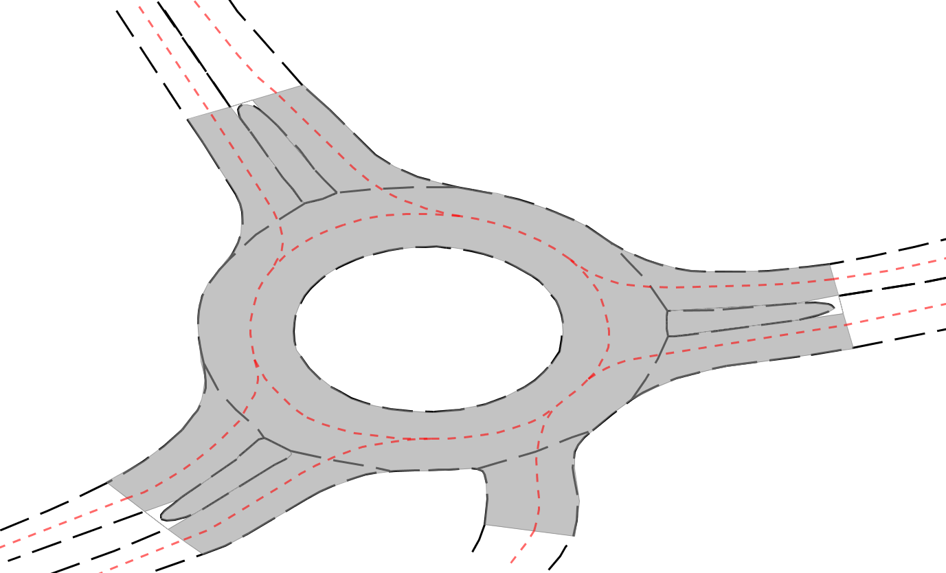
We provide the underlying HD map for each roundabout with included in the dataset. The map data is provided as shapefiles and an XMLfile and distinguishes three logical elements of the road topology: lane centerlines, lane boundaries, and drivable areas. For each such logical element, three shapefiles are provided, a .shp, a .shx, and a .dbf, resulting in a total of nine shapefiles included in the dataset per roundabout. The .shp file defines the underlying geometry of the logical element, such as the points of the lanes. The .dbf attribute files are in dBase format and define element-specific attributes. For the lane centerlines, the .dbf file contains, among other attributes, a unique identifier for each lane centerline and a list of succeeding lane centerlines, preceding lane centerlines, and parallel lane centerlines. The .dbf file for the lane boundaries defines the corresponding lane identifier, as well as the material of the lane boundary, such as CONCRETE for a curbstone and NONE for an implicit lane boundary. The .shx file is an index file of the shape geometry .shp file, providing a way to quickly iterate over the defined geometry. An exemplary visualisation of the provided shapefiles is given in Fig. 3. In addition to the shapefiles we also provide an .XML file for each intersection , representing the information contained in the shapefiles in a non-binary format that can be easily parsed by most programming languages.
Beyond the HD map and object states, the dataset includes a geo-referenced and anonymized example picture taken from the drone perspective of each intersection . This picture both provides a way of visualizing the trajectory data, as well as a supplementary input to the provided HD map.
III-A Dataset Statistics
The dataset was recorded at different times of day, for each roundabout including at least at the rush hour times in the morning and afternoon, as well as regular intervals in between rush hours.
The dataset spans , of which cover the first roundabout and the remaining are distributed among the remaining six roundabouts to , with varying lengths around for each. An example picture of each roundabout is depicted in Fig. 2. In total trajectories are included in the dataset, covering . A detailed overview of the openDD dataset, distinguishing between the seven different roundabouts included in the dataset, is provided in Table II. Here, the number of trajectories, the average trajectory duration, length, velocity, and total acceleration is stated for each object class, as well as for each roundabout. The average trajectory duration over all classes and all data subsets is , with an average trajectory length of .
The average velocity is and the average total acceleration is .
The relatively high amount of vehicles, cross the whole dataset, compared to the edestrians and bicyclists, is caused by the high percentage of covered rush hour times, as well as the remote locations of some of the covered roundabouts. The roundabout has an especially high traffic load with nique vehicles passing the roundabout in .
Roundabout has a very high average trajectory duration of pedestrians, with compared to the average pedestrian trajectory duration of . The high pedestrian trajectory duration of is caused by several pedestrians idling in the recordings of .
IV Using the Dataset
Publications of trajectory prediction models that use this dataset should be evaluated in a uniform fashion. To this end we define metrics to evaluate predicted trajectories, different splits of the openDD dataset, and propose several challenges using this dataset in the following.
| Data Subset | all | |||||||
| Recorded time | ||||||||
| # drone flights | ||||||||
| # trajectories | ||||||||
| passenger cars | ||||||||
| van | ||||||||
| truck | ||||||||
| bus | ||||||||
| pedestrian | ||||||||
| trailer | ||||||||
| motorcycle | ||||||||
| biyclist | ||||||||
| Average trajectory duration | ||||||||
| passenger cars | ||||||||
| van | ||||||||
| truck | ||||||||
| bus | ||||||||
| pedestrian | ||||||||
| trailer | ||||||||
| motorcycle | ||||||||
| biyclist | ||||||||
| Average trajectory length | ||||||||
| passenger cars | ||||||||
| van | ||||||||
| truck | ||||||||
| bus | ||||||||
| pedestrian | ||||||||
| trailer | ||||||||
| motorcycle | ||||||||
| biyclist | ||||||||
| Average velocity | ||||||||
| passenger cars | ||||||||
| van | ||||||||
| truck | ||||||||
| bus | ||||||||
| pedestrian | ||||||||
| trailer | ||||||||
| motorcycle | ||||||||
| biyclist | ||||||||
| Average acceleration | ||||||||
| passenger cars | ||||||||
| van | ||||||||
| truck | ||||||||
| bus | ||||||||
| pedestrian | ||||||||
| trailer | ||||||||
| motorcycle | ||||||||
| biyclist | ||||||||
IV-A Distance Metrics
Similar to our previous work [3], we define several distance metrics that can be used to evaluate the accuracy of a trajectory prediction algorithm. For a given object with index , this distance metric compares the predicted trajectory with the actual ground truth trajectory of the object, as given in the dataset. In the example scripts that are made available with the dataset, implementations of the used metrics are provided.
Euclidean displacement at time : The Euclidean point-to-point distance between the -th trajectory point of and the -th trajectory point of is defined as
| (2) |
Mean-squared Euclidean distance: Given two trajectories , spanning the same sequence of time instants , the mean squared Euclidean distances between the two entire trajectories is defined as the normalized sum of the squared Euclidean distances between the points corresponding to the same time instant :
| (3) |
Modified Hausdorff (MH) distance: The following definition of the modified Hausdorff (MH)distance is adopted from a work on object matching by Dubuisson et al. [13].
The definition of the point-to-set distance between the -th point of a trajectory , and another entire trajectory , is:
| (4) |
| Subset | |||||||||||
| train | val | train | val | train | val | ||||||
| Recorded time | |||||||||||
| # recordings from | |||||||||||
| 130 | 107 | 23 | 0 | 0 | 107 | 23 | 23 | 23 | 0 | 23 | |
| 48 | 40 | 8 | 40 | 8 | 40 | 8 | 8 | 8 | 0 | 8 | |
| 0 | 0 | 0 | 0 | 0 | 0 | 0 | 54 | 0 | 54 | 8 | |
| 59 | 49 | 10 | 49 | 10 | 49 | 10 | 10 | 10 | 0 | 10 | |
| 51 | 42 | 9 | 42 | 9 | 42 | 9 | 9 | 9 | 0 | 9 | |
| 44 | 36 | 8 | 36 | 8 | 0 | 0 | 8 | 8 | 0 | 8 | |
| 48 | 39 | 9 | 39 | 9 | 39 | 9 | 9 | 9 | 0 | 9 | |
The directed modified Hausdorff (DMH) distance is defined by Dubuisson et al. [13] as
| (5) |
The undirected, modified Hausdorff (MH) distance is then computed by taking the maximum over the two directed distances:
| (6) |
The MHdistance captures the spatial similarity of the trajectories without considering temporal misalignments. For example, two trajectories encoding the same path traveled at different velocities would have a low MHdistance, while their Euclidean displacement and mean squared Euclidean distance would be high.
IV-B Dataset Splits
We divide the drone recordings of the seven roundabouts into subsets for training, validation, and testing, as specified in Table III. The exact assignment of recordings to the different subsets introduced in the following, defining which recording belongs to which subset, is provided in the dataset.
For testing purposes, we use all recordings from , as well as of the recordings from the other roundabouts making up the total test set . We define three different subsets of the total test set to evaluate algorithms on: , , .
The subset includes all recordings in , but the ones of , thus it includes from all roundabouts with . The second subset covers all recordings of . Lastly, includes from the recordings of , as well as all recordings from the other roundabouts included in , such that in total of each roundabout are covered by this test set.
For training purposes, from the entire data we split the recordings not included in into three different splits . To define the splits , we split the data included in for the roundabouts , such that around of the recordings of each roundabout, except , form the validation set and the remaining the training set. For the first split we include the training and validation subsets formed in this way for all the roundabouts included in . The second split , and third split are equal to , but leave out all recordings from and , respectively.
An important feature of this proposed division of the dataset is that the splits can be combined with any of the test sets and to analyze different aspects of the learning process. The test set only includes recordings for topologies that are also included in , allowing for an evaluation of the model’s ability to predict trajectories for previously seen roundabout topologies. The test set includes only recordings from an unseen roundabout, thus it is suitable to evaluate the generalization capability of the learned model. Especially a combination with the split is of interest, since does not include the data of , which is the only other roundabout with a similar topology including lanes to skip the center roundabout lane. Lastly, the test set is a mixture between the other two test sets, enabling an evaluation of both the learning capacity of the model, as well as its generalization ability.
IV-C Challenges
We encourage all publications using the openDD dataset to report their results using the Euclidean displacement as defined in (2), and the MHas defined in (6) at the maximal prediction horizon they are reporting, and after , , and , if applicable.
Along the lines of our previous work [3], we propose to investigate the utility of the various information of the environment provided in the dataset. Thus, we invite parties interested in using the dataset to adopt their algorithms for trajectory prediction in such a way that they can work with variable input data.
Out of the possible nine combinations between the three test sets , and and the training and validation splits , we encourage researchers using the dataset to report the results of the following four combinations, with the first two being the most relevant.
Train on , test on : All roundabout topologies tested upon have been seen during the training. Thus the results on this combination will measure the general capability of the model to solve the task at hand.
Train on , test on : The test set only includes data covering a previously unseen roundabout, this combination can be used to assess the generalization capability of the evaluated model.
Train on , test on : Only recordings from a previously unseen roundabout, are included in the test set. Additionally, no recordings from the roundabout with the road topology most similar to the one of the test roundabout, is included in . This combination represents an even more difficult generalization evaluation.
Train on , test on : No recordings from , the roundabout which covers almost , is included in . Recordings from both seen and unseen roundabouts is included in the test set. This allows for an evaluation of both the capability of the model as well as the generalization ability and has an almost balanced amount of hours covered for each roundabout in .
Beyond the reporting of the aforementioned measures and training/testing splits, we propose three further research challenges for trajectory prediction using the openDD dataset:
- 1.
Evaluation of the benefit of knowledge of the movement of other objects up to time instant .
- 2.
Evaluation of the benefit of the provided map data, divided by centerlines, lane boundaries and drivable areas. Here, a separate evaluation with the same algorithm using all of the provided information, only centerlines, and only drivable areas is desirable.
- 3.
Given the image of each intersection provided in the dataset is used by the trajectory prediction algorithm, we would like the authors to evaluate the benefit of the image. The image can be for example used as an input for a convolutional neural network (CNN), and be combined with a birds-eye view of the current traffic scene, implicitly encoding the structure of the surroundings [3].
If challenge 3) shows that the information provided by the image gives additional benefits for the trajectory prediction task, interesting follow-up research would deal with how to integrate this information into the HD map.
V FUTURE WORK
The openDD dataset introduced in this work is the biggest published trajectory dataset recorded from a drone perspective as of today. In addition to its length of over , it covers varying roundabout topologies, which makes it also valuable to study the generalization of trajectory prediction algorithms trained on it. The license of the provided openDD dataset, covering commercial and non-commercial usage, makes it appealing to both research institutions, as well as to companies. In a future publication we plan to provide a baseline on the given dataset, addressing the challenges introduced in Section IV.
VI ACKNOWLEDGMENT
The authors would like to thank all partners within the H2020 co-funded project L3Pilot — grant agreement number 723051 — for their cooperation in making this dataset available online. Responsibility for the information and views set out in this publication lies entirely with the authors.
References
- [1] D. Ridel, E. Rehder, M. Lauer, C. Stiller, and D. Wolf, “A Literature Review on the Prediction of Pedestrian Behavior in Urban Scenarios,” in Proc. of ITSC, Maui, HI, USA, Nov. 2018, pp. 3105–3112.
- [2] H. Cui, V. Radosavljevic, F.-C. Chou, T.-H. Lin, T. Nguyen, T.-K. Huang, J. Schneider, and N. Djuric, “Multimodal Trajectory Predictions for Autonomous Driving Using Deep Convolutional Networks,” arXiv:1809.10732, Sep. 2018. [Online]. Available: http://arxiv.org/abs/1809.10732
- [3] A. Breuer, S. Elflein, T. Joseph, J. Bolte, S. Homoceanu, and T. Fingscheidt, “Analysis of the Effect of Various Input Representations for LSTM-Based Trajectory Prediction,” in Proc. of ITSC, Auckland, New Zealand, Oct. 2019, pp. 2728–2735.
- [4] H. Cui, T. Nguyen, F.-C. Chou, T.-H. Lin, J. Schneider, D. Bradley, and N. Djuric, “Deep Kinematic Models for Physically Realistic Prediction of Vehicle Trajectories,” arXiv:1908.00219, Aug. 2019. [Online]. Available: http://arxiv.org/abs/1908.00219
- [5] K. Driggs-Campbell, V. Govindarajan, and R. Bajcsy, “Integrating Intuitive Driver Models in Autonomous Planning for Interactive Maneuvers,” in Proc. of ITSC, vol. 18, Yokohama, Japan, Dec. 2017, pp. 3461–3472.
- [6] “Enable-S3 Consortium.” [Online]. Available: https://www.enable-s3.eu/
- [7] A. Robicquet, A. Sadeghian, A. Alahi, and S. Savarese, “Learning Social Etiquette: Human Trajectory Understanding in Crowded Scenes,” in Proc. of ECCV, Amsterdam, The Netherlands, Oct. 2016, pp. 549–565.
- [8] R. Krajewski, J. Bock, L. Kloeker, and L. Eckstein, “The highD Dataset: A Drone Dataset of Naturalistic Vehicle Trajectories on German Highways for Validation of Highly Automated Driving Systems,” arXiv:1810.05642v1, Oct. 2018. [Online]. Available: https://arxiv.org/abs/1810.05642v1
- [9] D. Yang, L. Li, K. Redmill, and Ü. Özgüner, “Top-View Trajectories: A Pedestrian Dataset of Vehicle-Crowd Interaction from Controlled Experiments and Crowded Campus,” in Proc. of IV, Paris, France, Jun. 2019, pp. 899–904.
- [10] J. Bock, R. Krajewski, T. Moers, S. Runde, L. Vater, and L. Eckstein, “The inD Dataset: A Drone Dataset of Naturalistic Road User Trajectories at German Intersections,” 1911.07602, Nov. 2019. [Online]. Available: https://arxiv.org/abs/1911.07602
- [11] Z. Wei, L. Sun, D. Wang, H. Shi, A. Clausse, M. Naumann, J. Kummerle, H. Konigshof, C. Stiller, A. d. L. Fortelle, and M. Tomizuka, “INTERACTION Dataset: An INTERnational, Adversarial and Cooperative moTION Dataset in Interactive Driving Scenarios With Semantic Maps,” arXiv: 1910.03088, Sep. 2019. [Online]. Available: https://arxiv.org/abs/1910.03088
- [12] F. Poggenhans, J. Pauls, J. Janosovits, S. Orf, M. Naumann, F. Kuhnt, and M. Mayr, “Lanelet2: A High-Definition Map Framework for the Future of Automated Driving,” in Proc. of ITSC, Maui, HI, USA, Nov. 2018, pp. 1672–1679.
- [13] M. Dubuisson and A. K. Jain, “A Modified Hausdorff Distance for Object Matching,” in Proc. of ICPR, vol. 1, Jerusalem, Israel, Oct. 1994, pp. 566–568.
*