Measurement of High Energy Gamma Rays from
to
with the Alpha Magnetic Spectrometer on the International Space Station
Von der Fakultät für Mathematik, Informatik und Naturwissenschaften der RWTH Aachen University zur Erlangung des akademischen Grades eines Doktors der Naturwissenschaften genehmigte Dissertation
vorgelegt von
Dipl. Phys.
Bastian Beischer
aus Norden
| Berichter: | Universitätsprofessor Prof. Dr. Stefan Schael |
| Universitätsprofessor Prof. Dr. Christopher Wiebusch |
Tag der mündlichen Prüfung: 17.06.2020
Diese Dissertation ist auf den Internetseiten der Universitätsbibliothek online verfügbar.
Abstract
Measurement of High Energy Gamma Rays from to with the Alpha Magnetic Spectrometer on the International Space Station
In this thesis a measurement of the high energy -ray flux between and with the Alpha Magnetic Spectrometer is presented. The Alpha Magnetic Spectrometer (AMS-02) is a multi-purpose particle detector mounted externally on the International Space Station. AMS-02 is continuously collecting scientific data since its installation in May 2011.
Although primarily designed for the measurement of charged cosmic rays AMS-02 is capable of measuring high energy -rays in two complementary modes. The large background of charged particles is overcome with the help of the excellent particle detection efficiency of the detector.
In the first mode the electron and positron pair from a photon conversion in the upper part of the detector is reconstructed with the help of the silicon tracker. In this mode the photon direction is estimated from the two trajectories and its energy is inferred from the curvature of the two tracks in the AMS magnetic field.
In the second mode the photon passes through almost the entire detector and produces an electromagnetic shower in the calorimeter at the bottom of the experiment. In this case photon direction and energy are estimated from the properties of the shower.
Two independent analyses are presented in this thesis, one for each of the two modes. The event selection criteria and the associated resolution functions are presented in detail. The effective area is estimated from a full detector Monte-Carlo simulation and corrected for the most important differences between data and simulation. A full sky model for -rays is constructed from diffuse emission predictions and recent -ray source catalogs. A dedicated analysis of Fermi-LAT data is performed to fully enable a detailed comparison with the AMS result.
The measured flux of -rays is presented for various parts of the sky, including comparisons with Fermi-LAT data and with the constructed model. The inner galaxy is studied in detail, as an example of a region in which the photon flux is dominated by diffuse emission. The fluxes of several -ray producing sources, including Vela, Geminga and the Crab pulsar are shown. The Geminga pulsar is studied in detail, revealing its pulsed emission of -rays in the AMS-02 data, which allows to measure its frequency of rotation and to estimate its magnetic field strength and age. Finally, AMS-02 observed an outburst of the flaring blazar CTA-102 at the end of 2016.
These important AMS-02 results represent the first independent test of the Fermi-LAT data in the energy range from to .
Zusammenfassung
Messung von hoch-energetischer Gammastrahlung von bis mit dem Alpha Magnet Spektrometer auf der Internationalen Raumstation
In dieser Arbeit wird eine Messung des hoch-energetischen -ray Flusses zwischen und mit dem Alpha Magnet Spektrometer vorgestellt. Das Alpha Magnet Spektrometer (AMS-02) ist ein Mehrzweck-Teilchendetektor, welcher extern auf der Internationalen Raumstation angebracht ist. Seit seiner Installation im Mai 2011 zeichnet AMS-02 kontinuierlich wissenschaftliche Daten auf.
Obwohl AMS-02 primär für die Messung von geladener kosmischer Strahlung konzipiert wurde, ist es in der Lage hoch-energertische -Strahlung auf zwei komplementäre Arten zu messen. Der große Untergrund an geladenen Teilchen wird mit Hilfe der exzellenten Teilchennachweiseffizienz des Detektors unterdrückt.
Im ersten Modus werden die Spuren je eines Elektrons und eines Positrons aus einer Photonkonversion im oberen Detektor mit dem Siliziumspurdetektor rekonstruiert. Dabei wird die Photonrichtung aus den beiden Trajektorien bestimmt und die Energie des Photons über die Krümmung der beiden Spuren im AMS Magnetfeld gemessen.
Im zweiten Modus passieren Photonen fast den gesamten Detektor und produzieren dann im Kalorimeter einen elektromagnetischen Schauer am unteren Ende des Experiments. In diesem Fall werden die Photonrichtung und Energie aus den Eigenschaften des Schauers bestimmt.
Zwei unabhängige Analysen werden in dieser Arbeit vorgestellt, eine für jeden der beiden Modi. Die Ereignisselektionskriterien werden dargelegt und die dazugehörigen Auflösungsfunktionen im Detail bestimmt. Die effektive Fläche wird aus einer Monte-Carlo Simulation des gesamten Detektors berechnet und die größten Unterschiede zwischen Daten und Simulation werden korrigiert. Ein Modell der -Strahlung, welches für den gesamten Himmel gültig ist, wird aus Vorhersagen für die diffuse Emission und aktuellen Katalogen von -Strahlungsquellen konstruiert. Eine dedizierte Analyse von Fermi-LAT Daten wird durchgeführt, um einen detaillierten Vergleich mit dem AMS Ergebnis zu ermöglichen.
Die gemessenen -ray Flüsse werden für verschiedene Regionen am Himmel vorgestellt und mit den Fermi-LAT Daten und dem konstruierten Modell verglichen. Die innere Galaxie, als Beispiel für eine Region in der die diffuse Emission dominiert, wird im Detail studiert. Die Flüsse von mehreren -Strahlung produzierenden Quellen (z.B. Vela, Geminga und der Pulsar im Krebsnebel) werden gezeigt. Im Besonderen wird der Geminga Pulsar untersucht, wodurch die gepulste Emission von -Strahlung in dem AMS Daten sichtbar wird. Daraus wird die Rotationsfrequenz, die Stärke des Magnetfeldes und das Alter des Pulsars ermittelt. Desweiteren hat AMS-02 einen Ausbruch des Blasaren CTA-102 Ende 2016 beobachtet.
Diese wichtigen AMS-02 Ergebnisse stellen den ersten unabhängigen Test der Fermi-LAT Daten im Energiebereich zwischen und dar.
Eidesstattliche Erklärung
Bastian Beischer erklärt hiermit, dass diese Dissertation und die darin dargelegten Inhalte die eigenen sind und selbstständig, als Ergebnis der eigenen originären Forschung, generiert wurden.
Hiermit erkläre ich an Eides statt
- 1.
Diese Arbeit wurde vollständig oder größtenteils in der Phase als Doktorand dieser Fakultät und Universität angefertigt;
- 2.
Sofern irgendein Bestandteil dieser Dissertation zuvor für einen akademischen Abschluss oder eine andere Qualifikation an dieser oder einer anderen Institution verwendet wurde, wurde dies klar angezeigt;
- 3.
Wenn immer andere eigene- oder Veröffentlichungen Dritter herangezogen wurden, wurden diese klar benannt;
- 4.
Wenn aus anderen eigenen- oder Veröffentlichungen Dritter zitiert wurde, wurde stets die Quelle hierfür angegeben. Diese Dissertation ist vollständig meine eigene Arbeit, mit der Ausnahme solcher Zitate;
- 5.
Alle wesentlichen Quellen von Unterstützung wurden benannt;
- 6.
Wenn immer ein Teil dieser Dissertation auf der Zusammenarbeit mit anderen basiert, wurde von mir klar gekennzeichnet, was von anderen und was von mir selbst erarbeitet wurde;
- 7.
Kein Teil dieser Arbeit wurde vor deren Einreichung veröffentlicht.
List of Publications
References
- 1 Aguilar, M., et al. Electron and Positron Fluxes in Primary Cosmic Rays Measured with the Alpha Magnetic Spectrometer on the International Space Station. Phys. Rev. Lett., Volume 113:121102 [2014].
- 2 Aguilar, M., et al. Observation of Complex Time Structures in the Cosmic-Ray Electron and Positron Fluxes with the Alpha Magnetic Spectrometer on the International Space Station. Phys. Rev. Lett., Volume 121:051102 [2018].
- 3 Räihä, T., et al. Monte Carlo simulations of the transition radiation detector of the AMS-02 experiment. Nuclear Instruments and Methods in Physics Research Section A: Accelerators, Spectrometers, Detectors and Associated Equipment, Volume 868:10 – 14 [2017].
- 4 Aguilar, M., et al. First Result from the Alpha Magnetic Spectrometer on the International Space Station: Precision Measurement of the Positron Fraction in Primary Cosmic Rays of 0.5–350 GeV. Phys. Rev. Lett., Volume 110:141102 [2013].
- 5 Accardo, L., et al. High Statistics Measurement of the Positron Fraction in Primary Cosmic Rays of 0.5–500 GeV with the Alpha Magnetic Spectrometer on the International Space Station. Phys. Rev. Lett., Volume 113:121101 [2014].
- 6 Aguilar, M., et al. Precision Measurement of the Flux in Primary Cosmic Rays from 0.5 GeV to 1 TeV with the Alpha Magnetic Spectrometer on the International Space Station. Phys. Rev. Lett., Volume 113:221102 [2014].
- 7 Aguilar, M., et al. Precision Measurement of the Proton Flux in Primary Cosmic Rays from Rigidity 1 GV to 1.8 TV with the Alpha Magnetic Spectrometer on the International Space Station. Phys. Rev. Lett., Volume 114:171103 [2015].
- 8 Aguilar, M., et al. Precision Measurement of the Helium Flux in Primary Cosmic Rays of Rigidities 1.9 GV to 3 TV with the Alpha Magnetic Spectrometer on the International Space Station. Phys. Rev. Lett., Volume 115:211101 [2015].
- 9 Aguilar, M., et al. Antiproton Flux, Antiproton-to-Proton Flux Ratio, and Properties of Elementary Particle Fluxes in Primary Cosmic Rays Measured with the Alpha Magnetic Spectrometer on the International Space Station. Phys. Rev. Lett., Volume 117:091103 [2016].
- 10 Aguilar, M., et al. Precision Measurement of the Boron to Carbon Flux Ratio in Cosmic Rays from 1.9 GV to 2.6 TV with the Alpha Magnetic Spectrometer on the International Space Station. Phys. Rev. Lett., Volume 117:231102 [2016].
- 11 Aguilar, M., et al. Observation of the Identical Rigidity Dependence of He, C, and O Cosmic Rays at High Rigidities by the Alpha Magnetic Spectrometer on the International Space Station. Phys. Rev. Lett., Volume 119:251101 [2017].
- 12 Aguilar, M., et al. Observation of New Properties of Secondary Cosmic Rays Lithium, Beryllium, and Boron by the Alpha Magnetic Spectrometer on the International Space Station. Phys. Rev. Lett., Volume 120:021101 [2018].
- 13 Aguilar, M., et al. Precision Measurement of Cosmic-Ray Nitrogen and its Primary and Secondary Components with the Alpha Magnetic Spectrometer on the International Space Station. Phys. Rev. Lett., Volume 121:051103 [2018].
- 14 Aguilar, M., et al. Observation of Fine Time Structures in the Cosmic Proton and Helium Fluxes with the Alpha Magnetic Spectrometer on the International Space Station. Phys. Rev. Lett., Volume 121:051101 [2018].
- 15 Aguilar, M., et al. Towards Understanding the Origin of Cosmic-Ray Positrons. Phys. Rev. Lett., Volume 122:041102 [2019].
- 16 Aguilar, M., et al. Towards Understanding the Origin of Cosmic-Ray Electrons. Phys. Rev. Lett., Volume 122:101101 [2019].
- 17 Aguilar, M., et al. Properties of Cosmic Helium Isotopes Measured by the Alpha Magnetic Spectrometer. Phys. Rev. Lett., Volume 123:181102 [2019].
- 18 Dodelson, S., et al. Constraining cosmological dark matter annihilation with gamma ray observations. Phys. Rev. D, Volume 80(8):083504–9 [2009].
- 19 Serpico, P. D. et al. Gamma rays from dark matter annihilation in the central region of the Galaxy. New Journal of Physics, Volume 11(10):105010 [2009].
- 20 Bringmann, T. et al. Gamma ray signals from dark matter: Concepts, status and prospects. Physics of the Dark Universe, Volume 1(1):194 – 217 [2012]. Next Decade in Dark Matter and Dark Energy.
- 21 Ackermann, M., et al. Searching for Dark Matter Annihilation from Milky Way Dwarf Spheroidal Galaxies with Six Years of Fermi Large Area Telescope Data. Phys. Rev. Lett., Volume 115(23):231301 [2015].
- 22 Ackermann, M., et al. Constraining Dark Matter Models from a Combined Analysis of Milky Way Satellites with the Fermi Large Area Telescope. Phys. Rev. Lett., Volume 107(24):241302 [2011].
- 23 Ackermann, M., et al. Fermi-LAT Observations of the Diffuse -Ray Emission: Implications for Cosmic Rays and the Interstellar Medium. The Astrophysical Journal, Volume 750(1):3 [2012].
- 24 Acero, F., et al. Development of the Model of Galactic Interstellar Emission for Standard Point-source Analysis of Fermi Large Area Telescope Data. The Astrophysical Journal Supplement Series, Volume 223(2):26 [2016].
- 25 Hooper, D. et al. Dark matter annihilation in the Galactic Center as seen by the Fermi Gamma Ray Space Telescope. Physics Letters B, Volume 697(5):412–428 [2011].
- 26 Daylan, T., et al. The characterization of the gamma-ray signal from the central Milky Way: A case for annihilating dark matter. Physics of the Dark Universe, Volume 12:1–23 [2016].
- 27 Ackermann, M., et al. The Fermi Galactic Center GeV Excess and Implications for Dark Matter. The Astrophysical Journal, Volume 840(1):43 [2017].
- 28 Su, M., et al. Giant Gamma-ray Bubbles from Fermi-LAT: Active Galactic Nucleus Activity or Bipolar Galactic Wind? ApJ, Volume 724(2):1044–1082 [2010].
- 29 Abbott, B. P., et al. GW170817: Observation of Gravitational Waves from a Binary Neutron Star Inspiral. Phys. Rev. Lett., Volume 119(16):161101 [2017].
- 30 IceCube Collaboration, et al. Multimessenger observations of a flaring blazar coincident with high-energy neutrino IceCube-170922A. Science, Volume 361(6398):eaat1378 [2018].
- 31 Kraushaar, W. L., et al. High-Energy Cosmic Gamma-Ray Observations from the OSO-3 Satellite. ApJ, Volume 177:341 [1972].
- 32 Fichtel, C. E., et al. High-energy gamma-ray results from the second Small Astronomy Satellite. ApJ, Volume 198:163–182 [1975].
- 33 Bignami, G. F., et al. The COS-B experiment for gamma-ray astronomy. Space Science Instrumentation, Volume 1:245–268 [1975].
- 34 Hartman, R. C., et al. The EGRET High Energy Gamma Ray Telescope. In NASA Conference Publication, Volume 3137 of NASA Conference Publication, pages 116–125 [1992].
- 35 Hartman, R. C., et al. The Third EGRET Catalog of High-Energy Gamma-Ray Sources. ApJS, Volume 123(1):79–202 [1999].
- 36 Hunter, S. D., et al. EGRET Observations of the Diffuse Gamma-Ray Emission from the Galactic Plane. ApJ, Volume 481(1):205–240 [1997].
- 37 Meegan, C. A., et al. Spatial distribution of -ray bursts observed by BATSE. Nature, Volume 355(6356):143–145 [1992].
- 38 Schoenfelder, V., et al. Instrument Description and Performance of the Imaging Gamma-Ray Telescope COMPTEL aboard the Compton Gamma-Ray Observatory. ApJS, Volume 86:657 [1993].
- 39 Atwood, W. B. et al. The Large Area Telescope on the Fermi Gamma-ray Space Telescope Mission [2009].
- 40 Meegan, C., et al. The Fermi Gamma-ray Burst Monitor. ApJ, Volume 702(1):791–804 [2009].
- 41 Ferenc, D. et al. The MAGIC gamma-ray observatory. Nuclear Instruments and Methods in Physics Research A, Volume 553(1-2):274–281 [2005].
- 42 Hinton, J. A. et al. The status of the HESS project. New A Rev., Volume 48(5-6):331–337 [2004].
- 43 Weekes, T. C., et al. VERITAS: the Very Energetic Radiation Imaging Telescope Array System. Astroparticle Physics, Volume 17(2):221–243 [2002].
- 44 Actis, M., et al. Design concepts for the Cherenkov Telescope Array CTA: an advanced facility for ground-based high-energy gamma-ray astronomy. Experimental Astronomy, Volume 32(3):193–316 [2011].
- 45 Atwood, W. B., et al. The Large Area Telescope on the Fermi Gamma-Ray Space Telescope Mission. The Astrophysical Journal, Volume 697(2):1071 [2009].
- 46 Kounine, A., et al. Precision measurement of 0.5 GeV - 3 TeV electrons and positrons using the AMS Electromagnetic Calorimeter. Nuclear Instruments and Methods in Physics Research Section A: Accelerators, Spectrometers, Detectors and Associated Equipment, Volume 869:110 – 117 [2017].
- 47 Adloff, C., et al. The AMS-02 lead-scintillating fibres Electromagnetic Calorimeter. Nuclear Instruments and Methods in Physics Research Section A: Accelerators, Spectrometers, Detectors and Associated Equipment, Volume 714:147 – 154 [2013].
- 48 Ackermann, M., et al. In-flight measurement of the absolute energy scale of the Fermi Large Area Telescope. Astroparticle Physics, Volume 35(6):346 – 353 [2012].
- 49 Abdollahi, S., et al. Cosmic-ray electron-positron spectrum from 7 GeV to 2 TeV with the Fermi Large Area Telescope. Phys. Rev. D, Volume 95:082007 [2017].
- 50 Ackermann, M., et al. Detection of the Characteristic Pion-Decay Signature in Supernova Remnants. Science, Volume 339(6121):807–811 [2013].
- 51 Tsai, Y.-S. Pair production and bremsstrahlung of charged leptons. Rev. Mod. Phys., Volume 46:815–851 [1974].
- 52 Landau, L. D. et al. Limits of applicability of the theory of bremsstrahlung electrons and pair production at high-energies. Dokl. Akad. Nauk Ser. Fiz., Volume 92:535 [1953].
- 53 Migdal, A. B. Bremsstrahlung and Pair Production in Condensed Media at High Energies. Phys. Rev., Volume 103:1811–1820 [1956].
- 54 Tanabashi, M., et al. Review of Particle Physics. Phys. Rev. D, Volume 98:030001 [2018].
- 55 Klein, O. et al. Über die Streuung von Strahlung durch freie Elektronen nach der neuen relativistischen Quantendynamik von Dirac. Zeitschrift für Physik, Volume 52(11):853–868 [1929].
- 56 Cheng, K. S. et al. The Synchrotron Self-Compton Model for X-Ray and gamma -Ray Emission from Pulsars. ApJ, Volume 448:281 [1995].
- 57 Jóhannesson, G., et al. The Three-dimensional Spatial Distribution of Interstellar Gas in the Milky Way: Implications for Cosmic Rays and High-energy Gamma-ray Emissions. The Astrophysical Journal, Volume 856(1):45 [2018].
- 58 Aguilar, M. et al. Cosmic-ray positron fraction measurement from 1-GeV to 30- GeV with AMS-01. Phys. Lett., Volume B646:145–154 [2007].
- 59 Adriani, O. et al. An anomalous positron abundance in cosmic rays with energies 1.5.100 GeV. Nature, Volume 458:607–609 [2009].
- 60 Hooper, D., et al. Excesses in cosmic ray positron and electron spectra from a nearby clump of neutralino dark matter. Phys. Rev. D., Volume 79:103513 [2009].
- 61 Hooper, D., et al. Pulsars as the sources of high energy cosmic ray positrons. Journal of Cosmology and Astroparticle Physics, Volume 2009(01):025 [2009].
- 62 Pierre Auger Collaboration. The Pierre Auger Cosmic Ray Observatory. Nuclear Instruments and Methods in Physics Research A, Volume 798:172–213 [2015].
- 63 Adriani, O., et al. PAMELA Measurements of Cosmic-Ray Proton and Helium Spectra. Science, Volume 332(6025):69–72 [2011].
- 64 Chang, J., et al. The DArk Matter Particle Explorer mission. Astroparticle Physics, Volume 95:6–24 [2017].
- 65 D. A. M. P. E. Collaboration, et al. Measurement of the cosmic ray proton spectrum from 40 GeV to 100 TeV with the DAMPE satellite. Science Advances, Volume 5(9) [2019].
- 66 Strong, A. W. et al. Propagation of Cosmic-Ray Nucleons in the Galaxy. The Astrophysical Journal, Volume 509(1):212–228 [1998].
- 67 Strong, A. W., et al. The GALPROP code for cosmic-ray transport and diffuse emission production., https://galprop.stanford.edu.
- 68 Torii, S. et al. Calorimetric electron telescope mission. Search for dark matter and nearby sources. Nuclear Instruments and Methods in Physics Research A, Volume 630(1):55–57 [2011].
- 69 Adriani, O., et al. Energy Spectrum of Cosmic-Ray Electron and Positron from 10 GeV to 3 TeV Observed with the Calorimetric Electron Telescope on the International Space Station. Phys. Rev. Lett., Volume 119:181101 [2017].
- 70 Aharonian, F., et al. Probing the ATIC peak in the cosmic-ray electron spectrum with H.E.S.S. Astronomy and Astrophysics, Volume 508(2):561–564 [2009].
- 71 Aharonian, F., et al. Energy Spectrum of Cosmic-Ray Electrons at TeV Energies. Phys. Rev. Lett., Volume 101(26):261104 [2008].
- 72 D. A. M. P. E. Collaboration, et al. Direct detection of a break in the teraelectronvolt cosmic-ray spectrum of electrons and positrons. Nature, Volume 552:63 [2017].
- 73 S. W. Barwick, e. a. Measurements of the Cosmic-Ray Positron Fraction from 1 to 50 GeV. The Astrophysical Journal Letters, Volume 482(2):L191– [1997].
- 74 Cirelli, M. et al. Minimal Dark Matter predictions and the PAMELA positron excess [2008].
- 75 Chowdhury, D., et al. Results from PAMELA, ATIC and FERMI : Pulsars or Dark Matter ? [2009].
- 76 Ando, S., et al. Dark matter annihilation or unresolved astrophysical sources? Anisotropy probe of the origin of cosmic gamma-ray background. Phys. Rev., Volume D75:063519 [2007].
- 77 Kalberla, P. M. W., et al. The Leiden/Argentine/Bonn (LAB) Survey of Galactic HI - Final data release of the combined LDS and IAR surveys with improved stray-radiation corrections. A&A, Volume 440(2):775–782 [2005].
- 78 HI4PI Collaboration:, et al. HI4PI: a full-sky H I survey based on EBHIS and GASS. A&A, Volume 594:A116 [2016].
- 79 Sofue, Y. Dark halos of M 31 and the Milky Way. Publications of the Astronomical Society of Japan, Volume 67(4) [2015].
- 80 He, C., et al. The Correlation between Dispersion Measure and X-Ray Column Density from Radio Pulsars. The Astrophysical Journal, Volume 768(1):64 [2013].
- 81 Freudenreich, H. T. A COBE Model of the Galactic Bar and Disk. The Astrophysical Journal, Volume 492(2):495–510 [1998].
- 82 Porter, T. A., et al. High-energy Gamma Rays from the Milky Way: Three-dimensional Spatial Models for the Cosmic-Ray and Radiation Field Densities in the Interstellar Medium. The Astrophysical Journal, Volume 846(1):67 [2017].
- 83 Robitaille, T.P., et al. A self-consistent model of Galactic stellar and dust infrared emission and the abundance of polycyclic aromatic hydrocarbons. A&A, Volume 545:A39 [2012].
- 84 Sodroski, T. J., et al. A Three-dimensional Decomposition of the Infrared Emission from Dust in the Milky Way. The Astrophysical Journal, Volume 480(1):173–187 [1997].
- 85 Miville-Deschenes, M.-A. et al. IRIS: A New Generation of IRAS Maps. The Astrophysical Journal Supplement Series, Volume 157(2):302–323 [2005].
- 86 Fazio, G. G., et al. The Infrared Array Camera (IRAC) for theSpitzer Space Telescope. The Astrophysical Journal Supplement Series, Volume 154(1):10–17 [2004].
- 87 Aeronautics, N. et al. A Giant Hubble Mosaic of the Crab Nebula [2005], https://hubblesite.org/contents/media/images/2005/37/1823-Image.html.
- 88 Shklovskii, I. S. On the Nature of the Optical Emission from the Crab Nebula. Soviet Ast., Volume 1:690 [1957].
- 89 Chandrasekhar, S. The Maximum Mass of Ideal White Dwarfs. ApJ, Volume 74:81 [1931].
- 90 Tolman, R. C. Static Solutions of Einstein’s Field Equations for Spheres of Fluid. Physical Review, Volume 55(4):364–373 [1939].
- 91 Oppenheimer, J. R. et al. On Massive Neutron Cores. Physical Review, Volume 55(4):374–381 [1939].
- 92 Wikipedia. Schematic view of a pulsar [2007], https://commons.wikimedia.org/wiki/File:Pulsar_schematic.svg.
- 93 Aeronautics, N. et al. Combined X-Ray and Optical Images of the Crab Nebula [2002], https://hubblesite.org/contents/media/images/2002/24/1248-Image.html.
- 94 Harding, A. K. Gamma-ray Pulsars: Models and Predictions. AIP Conference Proceedings, Volume 558(1):115–126 [2001].
- 95 Condon, J. J. et al. Essential Radio Astronomy [2016].
- 96 Condon, James and Ransom, Scott. Essential Radio Astronomy, https://www.cv.nrao.edu/˜sransom/web/Ch6.html.
- 97 Drake, F. D. Radio Observations of the Crab Nebula Pulsar. In Davies, R. D. et al., editors, The Crab Nebula, Volume 46 of IAU Symposium, page 73 [1971].
- 98 Mattox, J. R., et al. SAS 2 Observation of Pulsed High-Energy Gamma Radiation from Geminga. ApJ, Volume 401:L23 [1992].
- 99 Abdo, A. A., et al. Fermi-LAT Observations of the Geminga Pulsar. The Astrophysical Journal, Volume 720(1):272 [2010].
- 100 McLaughlin, M. A. The North American Nanohertz Observatory for Gravitational Waves. Classical and Quantum Gravity, Volume 30(22):224008 [2013].
- 101 Anderson, P. W. et al. Pulsar glitches and restlessness as a hard superfluidity phenomenon. Nature, Volume 256(5512):25–27 [1975].
- 102 Australia Telescope National Facility. ATNF Glitch Database, https://www.atnf.csiro.au/research/pulsar/psrcat/glitchTbl.html.
- 103 Urry, C. M. et al. Unified Schemes for Radio-Loud Active Galactic Nuclei. PASP, Volume 107:803 [1995].
- 104 Aeronautics, N. et al. A Multi-Wavelength View of the Radio Galaxy Hercules A [2012], https://hubblesite.org/contents/media/images/2012/47/3110-Image.html.
- 105 Beckmann, V. et al. The AGN phenomenon: open issues. In Proceedings of “An INTEGRAL view of the high-energy sky (the first 10 years)” - 9th INTEGRAL Workshop and celebration of the 10th anniversary of the launch (INTEGRAL 2012). 15-19 October 2012. Bibliotheque Nationale de France, page 69 [2012].
- 106 Abdo, A. A., et al. Fermi Large Area Telescope Observations of Markarian 421: The Missing Piece of its Spectral Energy Distribution. The Astrophysical Journal, Volume 736(2):131 [2011].
- 107 Konopelko, A., et al. Modeling the TeV Gamma-Ray Spectra of Two Low-Redshift Active Galactic Nuclei: Markarian 501 and Markarian 421. The Astrophysical Journal, Volume 597(2):851–859 [2003].
- 108 Su, M., et al. Giant Gamma-Ray Bubbles from Fermi-LAT: Active Galactic Nucleus Activity or Bipolar Galactic Wind? The Astrophysical Journal, Volume 724(2):1044–1082 [2010].
- 109 The Fermi-LAT collaboration. Fermi Large Area Telescope Fourth Source Catalog. arXiv e-prints, arXiv:1902.10045 [2019].
- 110 The Fermi-LAT collaboration. Galactic Interstellar Emission Model for the 4FGL Catalog Analysis, https://fermi.gsfc.nasa.gov/ssc/data/analysis/software/aux/4fgl/Galactic_Diffuse_Emission_Model_for_the_4FGL_Catalog_Analysis.pdf.
- 111 Ackermann, M., et al. The Spectrum of Isotropic Diffuse Gamma-Ray Emission between 100 MeV and 820 GeV. ApJ, Volume 799(1):86 [2015].
- 112 Acero, F., et al. Fermi Large Area Telescope Third Source Catalog. The Astrophysical Journal Supplement Series, Volume 218(2):23 [2015].
- 113 National Aeronautics and Space Administration. International Space Station Gallery, https://www.nasa.gov/mission_pages/station/images/station_post_construction/index.html.
- 114 Kounine, A. The Alpha Magnetic Spectrometer on the International Space Station. International Journal of Modern Physics E, Volume 21(08):1230005 [2012].
- 115 NASA. Visible Earth [2002], https://visibleearth.nasa.gov/view.php?id=57730.
- 116 National Aeronautics and Space Administration. The International Space Station’s coordinate system, https://www.nasa.gov/mission_pages/station/multimedia/iss_labs_guide.html.
- 117 National Aeronautics and Space Administration. Space Station Reference Coordinate Systems, https://pims.grc.nasa.gov/plots/user/tibor/SSP30219JISSCoordSystems.pdf.
- 118 Vondrák, J. et al. International Earth Rotation and Reference Systems Service (IERS) web: www.iers.org. Journal of Geodesy, Volume 77(10-11):585–678 [2004].
- 119 Petit, G. et al. IERS Conventions (2010). Verlag des Bundesamts für Kartographie und Geodäsie [2010].
- 120 Altamimi, Z., et al. ITRF2014: A new release of the International Terrestrial Reference Frame modeling nonlinear station motions. Journal of Geophysical Research: Solid Earth, Volume 121(8):6109–6131 [2016].
- 121 National Geospatial-Intelligence Agency - Office of Geomagnetics. Department of Defense (DoD) World Geodetic System (WGS) 1984 - Its Definition and Relationships with Local Geodetic Systems [2014].
- 122 Wikipedia. RA and Dec on celestial sphere [2012], https://en.wikipedia.org/wiki/File:Ra_and_dec_on_celestial_sphere.png.
- 123 Aeronautics, N. et al. General Mission Analysis Tool [2012], http://gmat.sourceforge.net/docs/nightly/files/images/Resource_CoordinateSystems_GUI_5.png.
- 124 Kaplan, G. The IAU Resolutions on Astronomical Reference Systems, Time Scales, and Earth Rotation Models: Explanation and Implementation. United States Naval Observatory Circular 179 [2005].
- 125 International Astronomical Union. IAU 1976 Resolution 1 [1976].
- 126 Fricke, W., et al. Fourth Fundamental Catalogue (FK4). Veröffentlichungen des Astronomischen Rechen-Instituts Heidelberg, Volume 10:1–144 [1963].
- 127 Fricke, W., et al. Fifth Fundamental Catalogue (FK5). Part 1. The Basic Fundamental Stars. Veröffentlichungen des Astronomischen Rechen-Instituts Heidelberg, Volume 32:1–106 [1988].
- 128 Perryman, M. A. C., et al. The Hipparcos Catalogue. Astronomy and Astrophysics, Volume 500:501–504 [1997].
- 129 Wielen, R., et al. Sixth Catalogue of Fundamental Stars (FK6). Part I. Basic fundamental stars with direct solutions. Veröffentlichungen des Astronomischen Rechen-Instituts Heidelberg, Volume 35 [1999].
- 130 Arias, E. F., et al. The extragalactic reference system of the International Earth Rotation Service, ICRS. Astronomy and Astrophysics, Volume 303:604–608 [1995].
- 131 Ma, C., et al. The International Celestial Reference Frame as Realized by Very Long Baseline Interferometry. The Astronomical Journal, Volume 116(1):516–546 [1998].
- 132 International Astronomical Union. IAU 1997 Resolution B2 [1997].
- 133 Mignard, F. et al. Linking the FK5 to the ICRF. Highlights of Astronomy, Volume 11:313 [1998].
- 134 Observatory, E. S. Artist’s impression of the Milky Way [2013], https://www.eso.org/public/images/eso1339e.
- 135 Blaauw, A., et al. The New I.A.U. System of Galactic Coordinates (1958 Revision). Monthly Notices of the Royal Astronomical Society, Volume 121(2):123–131 [1960].
- 136 Murray, C. A. The transformation of coordinates between the system of B1950.0 and J2000.0, and the principal galactic axes referred to J2000.0. Astronomy and Astrophysics, Volume 218:325–329 [1989].
- 137 Liu, J.-C., et al. Reconsidering the Galactic coordinate system. Astronomy & Astrophysics, Volume 526:A16 [2011].
- 138 Reid, M. J. et al. The Proper Motion of Sagittarius A*. II. The Mass of Sagittarius A*. The Astrophysical Journal, Volume 616(2):872–884 [2004].
- 139 The Astropy Collaboration, et al. The Astropy Project: Building an Open-science Project and Status of the v2.0 Core Package. The Astronomical Journal, Volume 156:123 [2018].
- 140 Vallado, D., et al. Revisiting Spacetrack Report #3. AIAA/AAS Astrodynamics Specialist Conference [2006].
- 141 Hoots, F. et al. Spacetrack Report No. 3 - Models for Propagation of NORAD Element Sets. United States Air Force Aerospace Defense Command [1980].
- 142 Magliacane, J. A. PREDICT: Satellite tracking and orbital prediction [2011].
- 143 Capitaine, N., et al. Definition of the Celestial Ephemeris Origin and of UT1 in the International Celestial Reference Frame. Astronomy and Astrophysics, Volume 355:398–405 [2000].
- 144 International Astronomical Union. IAU 2000 Resolution B1.8 [2000].
- 145 Capitaine, N., et al. Expressions for IAU 2000 precession quantities. Astronomy and Astrophysics, Volume 412(2):567–586 [2003].
- 146 International Astronomical Union. IAU 2000 Resolution B1.3 [2000].
- 147 International Astronomical Union. IAU 2000 Resolution B1.6 [2000].
- 148 Mathews, P. M., et al. Modeling of nutation and precession: New nutation series for nonrigid Earth and insights into the Earth’s interior. Journal of Geophysical Research: Solid Earth, Volume 107(B4):ETG 3–1–ETG 3–26 [2002].
- 149 International Astronomical Union. IAU 2006 Resolution B1 [2006].
- 150 Hilton, J. L., et al. Report of the International Astronomical Union Division I Working Group on Precession and the Ecliptic. Celestial Mechanics and Dynamical Astronomy, Volume 94(3):351–367 [2006].
- 151 Lieske, J. H., et al. Expressions for the Precession Quantities Based upon the IAU (1976) System of Astronomical Constants. Astronomy and Astrophysics, Volume 58:1–16 [1977].
- 152 Seidelmann, P. K. 1980 I.A.U. Theory of Nutation - the Final Report of the I.A.U. Working Group on Nutation. Celestial Mechanics, Volume 27(1):79–106 [1982].
- 153 IAU SOFA Board. IAU SOFA Software Collection [2019], http://www.iausofa.org.
- 154 AMS Collaboration. Alpha Magnetic Spectrometer Website, https://ams02.space.
- 155 Lübelsmeyer, K., et al. Upgrade of the Alpha Magnetic Spectrometer (AMS-02) for long term operation on the International Space Station (ISS). Nuclear Instruments and Methods in Physics Research Section A: Accelerators, Spectrometers, Detectors and Associated Equipment, Volume 654(1):639 – 648 [2011].
- 156 Berdugo, J., et al. Determination of the rigidity scale of the Alpha Magnetic Spectrometer. Nuclear Instruments and Methods in Physics Research Section A: Accelerators, Spectrometers, Detectors and Associated Equipment, Volume 869:10 – 14 [2017].
- 157 University of Geneva. AMS Tracker Integration and Assembly Pictures, http://dpnc.unige.ch/ams/ams_beta/Welcome_New.shtml.
- 158 Azzarello, P. Tests and production of the AMS-02 silicon tracker detectors. Ph.D. thesis, Geneva U. [2004].
- 159 Ambrosi, G., et al. The spatial resolution of the silicon tracker of the Alpha Magnetic Spectrometer. Nuclear Instruments and Methods in Physics Research Section A: Accelerators, Spectrometers, Detectors and Associated Equipment, Volume 869:29 – 37 [2017].
- 160 Bindi, V., et al. Calibration and performance of the AMS-02 time of flight detector in space. Nuclear Instruments and Methods in Physics Research Section A: Accelerators, Spectrometers, Detectors and Associated Equipment, Volume 743:22 – 29 [2014].
- 161 Bindi, V., et al. The scintillator detector for the fast trigger and time-of-flight (TOF) measurement of the space experiment AMS-02. Nuclear Instruments and Methods in Physics Research Section A: Accelerators, Spectrometers, Detectors and Associated Equipment, Volume 623(3):968 – 981 [2010].
- 162 von Doetinchem, P., et al. The AMS-02 Anticoincidence Counter. Nuclear Physics B - Proceedings Supplements, Volume 197(1):15 – 18 [2009]. 11th Topical Seminar on Innovative Particle and Radiation Detectors (IPRD08).
- 163 Goerres, A. Kalibration und Integration des AMS-02 Anti-Koinzidenz-Detektors. Diplomarbeit, RWTH Aachen [2010].
- 164 RWTH Aachen. AMS TRD Website, https://www1b.physik.rwth-aachen.de/˜schael/AMS_TRD.html.
- 165 Schael, Stefan. First six years of AMS on the ISS and future perspectives, https://www1b.physik.rwth-aachen.de/˜schael/AMS-100_files/2018_04_23_MPI.pdf.
- 166 Li, Z.-Y., et al. Antiproton identification below threshold with the AMS-02 RICH detector. Chinese Physics C, Volume 41(5):056001 [2017].
- 167 Giovacchini, F. Performance in space of the AMS-02 RICH detector. Nuclear Instruments and Methods in Physics Research Section A: Accelerators, Spectrometers, Detectors and Associated Equipment, Volume 766:57 – 60 [2014]. RICH2013 Proceedings of the Eighth International Workshop on Ring Imaging Cherenkov Detectors Shonan, Kanagawa, Japan, December 2-6, 2013.
- 168 Brun, R. et al. ROOT - An object oriented data analysis framework. Nuclear Instruments and Methods in Physics Research Section A: Accelerators, Spectrometers, Detectors and Associated Equipment, Volume 389(1):81 – 86 [1997].
- 169 Agostinelli, S., et al. Geant4–a simulation toolkit. Nuclear Instruments and Methods in Physics Research Section A: Accelerators, Spectrometers, Detectors and Associated Equipment, Volume 506(3):250–303 [2003].
- 170 Qu, Z., et al. New track finding based on cellar automaton for AMS-02 detector. Nuclear Instruments and Methods in Physics Research Section A: Accelerators, Spectrometers, Detectors and Associated Equipment, Volume 869:135 – 140 [2017].
- 171 Fermi-LAT. Fermi-LAT Performance [2016], http://www.slac.stanford.edu/exp/glast/groups/canda/lat_Performance.htm.
- 172 Sullivan, J. D. Geometrical factor and directional response of single and multi-element particle telescopes. Nuclear Instruments and Methods, Volume 95:5 [1971].
- 173 Hoecker, A., et al. TMVA: Toolkit for Multivariate Data Analysis. PoS, Volume ACAT:040 [2007].
- 174 D’Agostini, G. A multidimensional unfolding method based on Bayes’ theorem. Nuclear Instruments and Methods in Physics Research Section A: Accelerators, Spectrometers, Detectors and Associated Equipment, Volume 362(2):487 – 498 [1995].
- 175 Zimmermann, N. Precision measurement of the cosmic-ray electron and positron fluxes as a function of time and energy with the Alpha Magnetic Spectrometer on the International Space Station. Ph.D. thesis, RWTH Aachen University [2019].
- 176 Atwood, W., et al. Pass 8: Toward the Full Realization of the Fermi-LAT Scientific Potential. arXiv e-prints, arXiv:1303.3514 [2013].
- 177 Bruel, P., et al. Fermi-LAT improved Pass 8 event selection. arXiv e-prints, arXiv:1810.11394 [2018].
- 178 Ackermann, M., et al. The Fermi Large Area Telescope On Orbit: Event Classification, Instrument Response Functions, and Calibration. The Astrophysical Journal Supplement Series, Volume 203(1):4 [2012].
- 179 Górski, K. M., et al. HEALPix: A Framework for High-Resolution Discretization and Fast Analysis of Data Distributed on the Sphere. Astrophys. J., Volume 622:759–771 [2005].
- 180 Lafferty, G. et al. Where to stick your data points: The treatment of measurements within wide bins. Nuclear Instruments and Methods in Physics Research Section A: Accelerators, Spectrometers, Detectors and Associated Equipment, Volume 355(2):541 – 547 [1995].
- 181 Caraveo, P. A., et al. Parallax Observations with the Hubble Space Telescope Yield the Distance to Geminga. The Astrophysical Journal, Volume 461(2) [1996].
- 182 Yuksel, H., et al. TeV Gamma Rays from Geminga and the Origin of the GeV Positron Excess. Phys. Rev. Lett., Volume 103:051101 [2009].
- 183 Abeysekara, A. U., et al. Extended gamma-ray sources around pulsars constrain the origin of the positron flux at Earth. Science, Volume 358(6365):911–914 [2017].
- 184 Jet Propulsion Laboratory. Solar System Dynamics - Ephemerides, https://ssd.jpl.nasa.gov/?ephemerides.
- 185 Manchester, R. N., et al. The Australia Telescope National Facility Pulsar Catalogue. The Astronomical Journal, Volume 129(4):1993–2006 [2005].
- 186 Australia Telescope National Facility. ATNF Pulsar Catalogue, https://www.atnf.csiro.au/research/pulsar/psrcat.
- 187 The Fermi-LAT collaboration. LAT Gamma-ray Pulsar Timing Models, https://confluence.slac.stanford.edu/display/GLAMCOG/LAT+Gamma-ray+Pulsar+Timing+Models.
- 188 Ray, P. S., et al. Precise -ray Timing and Radio Observations of 17 Fermi -ray pulsars. The Astrophysical Journal Supplement Series, Volume 194(2):17 [2011].
- 189 Hobbs, G. B., et al. TEMPO2, a new pulsar-timing package - I. An overview. Monthly Notices of the Royal Astronomical Society, Volume 369(2):655–672 [2006].
- 190 Luo, J., et al. PINT: High-precision pulsar timing analysis package [2019].
- 191 Harris, D. E. et al. Radio Source Measurements at 960 Mc/s. Publications of the Astronomical Society of the Pacific, Volume 72:237 [1960].
- 192 Monroe, T. R., et al. The UV-Bright Quasar Survey (UVQS): DR 1. The Astronomical Journal, Volume 152(1):25 [2016].
- 193 Prince, R., et al. Fermi-Large Area Telescope Observations of the Brightest Gamma-Ray Flare Ever Detected from CTA 102. The Astrophysical Journal, Volume 866(1):16 [2018].
- 194 Shukla, A., et al. Short-timescale -Ray Variability in CTA 102. The Astrophysical Journal, Volume 854(2):L26 [2018].


The ACsoft software package, of which I am one of the principal authors, was used extensively for these publications (which were selected as Editor’s Suggestions):
- •
- •
My work on the Transition Radiation Detector of AMS has contributed to the following publication:
- •
My work for the successful operation of the TRD and of AMS as a whole was relevant for these publications:
- •
- •
- •
- •
- •
- •
- •
- •
- •
- •
- •
- •
- •
- •
\KOMAoptionsopen=right
Chapter 0 Introduction
The physics of high energy -rays is a gold mine for scientific discovery and full of unique possibilities. Since -rays form the high energy limit of electromagnetic radiation, they are associated with the most violent phenomena in the cosmos. It takes spectacular objects, such as pulsars or blazars to produce photons at and energies. In addition, new physics such as the ominous dark matter, is predicted to manifest itself in an excess of -rays in many models [18, 19, 20].
At the same time, because photons can pass through the universe almost undisturbed, they can be directly associated with their sources, making them the perfect messenger.
As an example, measurements of dwarf spheroidal galaxies provide some of the most stringent limits on the dark matter annihilation cross section[21, 22]. Because the photon energy does not change (which is in stark contrast to cosmic ray energies), -rays allow to search for line signatures of dark matter decays, which if detected, would allow to directly reconstruct the mass of the dark matter particle.
Gamma ray bursts (GRBs) are among the most violent and least understood phenomena in the universe. The enormous energy released within the course of a few seconds, manifests itself in massive -ray flares.
Within our own galaxy, the study of diffuse emission of -rays opens a new window to unveil the mysteries of cosmic rays[23, 24], which can otherwise only be studied in the vicinity of the solar system
Excess diffuse emission produced by the annihilation of dark matter particles, for example in the galactic center, is another topic that has sparked enormous interest [25, 26, 27]. Large scale structures of unknown origin, the Fermi bubbles [28] have been identified in the residuals and continue to puzzle astronomers.
Measurements of -rays have contributed to the discovery of gravitational waves [29], and to the association of a cosmic neutrinos with flaring blazars [30].
These are only some of the reasons why -ray astronomy is such a vital field.
On the other hand, experiments capable of studying -rays are relatively scarce. Because the Earth’s atmosphere is opaque to -radiation, experiments can be divided into two groups: Satellites in space, which directly observe the radiation, but are expensive to launch and operate, and telescopes on the Earth’s surface which indirectly measure the electromagnetic showers produced when the -ray hits the atmosphere. These telescopes are limited to the high energy end of the -ray spectrum, and suffer from a limited field of view.
| Experiment | Energy Range | Start of Operations |
|---|---|---|
| OSO-3 | - | 1967 |
| SAS-2 | - | 1972 |
| COS-B | - | 1975 |
| EGRET | - | 1991 |
| AGILE | - | 2007 |
| Fermi-LAT | - > | 2008 |
| AMS-02 | - | 2011 |
Table 1 provides a historic overview of -ray satellites. In the 1960s the OSO-3 satellite discovered the existence of cosmic -rays [31] and reported early measurements. In the 1970s, the satellites SAS-2 [32] and COS-B [33] were able to coarsely map the -ray sky and the first sources were identified and studied. This included the discovery of -ray pulsars, such as Geminga [32].
In the 1990s the EGRET[34] instrument on the Compton Gamma Ray Observatory (CGRO), part of NASA’s Great Observatories Program, was able to extend the list of sources [35] and to study diffuse emission [36] in some detail. The CGRO also contained the BATSE [37] and COMPTEL [38] instruments, which were specifically designed to study GRBs and to extend the lower energy reach of EGRET down to , respectively.
Nowadays, the most sensitive experiment by far is the Large Area Telescope (LAT) [39] on the Fermi satellite. The satellite is also equipped with a Gamma Ray Burst monitor (GBM) [40] for the detection of GRBs.

Figure 1 shows the improvement of the instrumental technique, starting with the SAS-2 satellite, all the way to the present day Fermi-LAT experiment. Both resolution and statistics improve as time progresses and more and more sources, structures and phenomena can be identified.
The experimental results from the Fermi-LAT instrument results have revolutionized -ray astronomy, with their unprecedented statistical accuracy and outstanding instrumental performance.
Even though cosmic photons at and energies can not be detected directly in ground based telescopes, there is a second class of experiments in which the Cherenkov light produced by relativistic particles in the atmospheric showers initiated by -rays is measured. Observatories which follow this approach are referred to as Imaging Atmospheric Cherenkov Telescopes (IACT).
These experiments generally observe photons at very high energies (VHE), with sensitivities which extend from approximately all the way to . The major Cherenkov telescopes currently in operation are MAGIC [41], H.E.S.S. [42] and VERITAS [43].
IACTs have excellent angular resolution and energy reach, with acceptable energy resolution. The major difference with respect to satellite based -ray experiments is that these telescopes can not be operated continuously and have a limited field of view. This means that they generally study specific point sources, and are not well suited for studies of large scale diffuse emission. This is also a disadvantage when trying to catch transient phenomena such as GRBs, since alert notifications from other experiments are required and time is needed to reorient the telescope.
It is interesting to note that bigger telescopes are required to extend the energy reach to lower energies. The Cherenkov Telescope Array (CTA) [44] is aiming to improve the lower energy limit down to , and will generally improve the sensitivity. It is currently under construction.
At the present time, there are only very few experiments which can measure photons in the energy range between and . In fact, there is only one experiment which covers the entirety of this energy range: The Fermi-LAT experiment.
Results obtained with the Fermi satellite have excellent statistical accuracy. But on the other hand the experiment, like any other, suffers from systematic uncertainties related to calibrations and imperfect understanding of the detector. Therefore, it is vital to have independent measurements as cross checks, in particular given the scientific relevance of the Fermi results.
The AMS-02 detector is a device which was built for the measurement of charged cosmic rays. It was installed as an external payload on the International Space Station (ISS) on May 19th 2011 and is operational ever since. It is designed as a multi- spectrometer in space and is supported by the efforts of more than 500 international scientists.
Although AMS was designed for charged cosmic ray measurements, the tracker and calorimeter of the experiment are also able to measure the properties of photons with outstanding precision. In addition, due to its excellent detection efficiency of charged cosmic rays, the AMS detector allows for a reliable reduction of charged particle backgrounds in -ray measurements.
The single photon pointing accuracy of the AMS-02 tracker is comparable to, and at high energies even better than, the Fermi-LAT pointing resolution. This is a result of the excellent single point resolution of the AMS tracker.
In addition, the AMS calorimeter is easily capable of measuring photons with energies, due to its 17 radiation length thickness. At these energies, calorimeter shower lateral leakage is a major problem in the Fermi-LAT calorimeter, and part of the reason why the energy reach was originally limited to [45] and only gradually increased later.
The resolution of the reconstructed energy in AMS calorimeter showers is outstanding [46]. The fine calorimeter granularity allows to reconstruct the photon direction with good accuracy [46]. In contrast to the Fermi-LAT calorimeter, the AMS flight model ECAL energy scale was calibrated in a dedicated test beam at CERN [47, 46]. The in flight absolute energy scale of the LAT has only been calibrated indirectly using electrons [48, 49].
Finally, the AMS detector was built with redundancy in mind. Because of this very important aspect, the photon analysis is possible in two complementary modes: With the tracker, using photons which converted in the upper detector, and with the calorimeter. These two modes are entirely complementary, which allows to reduce systematic uncertainties.
All these aspects make the AMS-02 detector very well suited for the measurement of high energy -rays.
Still, AMS measurements will not be able to compete with the Fermi-LAT satellite in terms of pure statistics, because of the limited acceptance of the detector in the two photon modes. But on the other hand, there are many regions of the sky in which the Fermi measurement is dominated by systematic uncertainties.
A good example is the inner galaxy, in which diffuse emission is the dominant process of -ray production. The study of these photons allows to infer enormous amounts of information about the galaxy and about cosmic rays, which is otherwise unavailable. It will be shown in this thesis that AMS can contribute significantly to the measurement of diffuse emission.
Spectra from strong -ray sources, such as Vela, Geminga and the Crab pulsar are other examples, in which AMS is able to add valuable information. AMS also surveys a sizable portion of the sky at any given time. For this reason it is well suited for the study of transient phenomena, in particular for the measurement of flaring sources.
In chapter 1 the ingredients to describe the high energy -ray sky will be assembled. This includes a short discussion of elementary processes relating to high energy photon physics. The charged cosmic ray fluxes, as well as the interstellar structure of gas and radiation fields in the Milky Way will be discussed. A short summary of a few important types of -ray sources will also be given. These ingredients will then be put together to form a predictive model of the -ray sky.
Chapter 2 will introduce the AMS-02 detector as the experimental apparatus whose measured data are the foundation for the analyses in this thesis. The detector is located on the International Space Station, which provides the operational support and the scientific environment for AMS. Both are described in detail, together with a review of astronomical coordinate systems and transformations.
The data and its analysis is explained in chapter 3. The chapter contains a description of the selection techniques and the response functions of the experiment, which include the angular and energy resolution functions and the effective area. The response functions are used to construct the exposure maps, which are in turn applied to the model of diffuse emission and -ray sources in order to construct photon count predictions maps for the entire sky. This chapter concludes with a discussion of a few necessary corrections to the photon Monte-Carlo simulation and an overview of the systematic uncertainties relevant to the analysis.
Chapter 4 contains a short description of a complementary Fermi-LAT analysis, which includes all necessary steps to construct photon fluxes from the publicly available Fermi-LAT data. It also includes an extensive discussion of Fermi-LAT systematic uncertainties.
Finally, the results for the photon fluxes in several regions of interest are presented and discussed in chapter 5, followed by a short summary in chapter 6.
Chapter 1 Understanding the -ray Sky
The observable -ray sky is a complex superposition of many different processes. In order to understand it, a complete picture of the structure and contents of the Milky Way must be combined with elementary particle physics, which describes the fundamental interactions of particles. In addition, some of the strongest -ray sources are violent extra galactic objects, such as blazars, which are extremely compact and are able to accelerate particles to the highest energies. These sources must also be incorporated in a realistic model.
In this chapter the fundamental processes relating to photons at the highest energies are described and combined with recent measurements of galactic gas and radiation field distributions in order to construct a model which can be compared to the AMS-02 data.
An overview of the physical processes for the production and detection of -rays will be given in section 1. These processes are generally well understood, because they can be studied in laboratories on Earth.
In order to predict the diffuse component of -rays it is important to understand the distribution of gas and radiation fields in the Milky Way. A short review of recent measurements and their results will be given in section 3.
Charged cosmic rays (CRs), such as a protons, electrons and particles are the projectiles which in turn interact with the interstellar matter and produce diffuse -rays. Therefore the flux and density of the most relevant cosmic ray species are needed for the calculation. In addition, cosmic rays are a major background in the detection of photons in the AMS-02 measurement. For these reasons a summary of recent cosmic ray measurement is given in section 2.
In addition to diffuse emission -rays are also produced in the vicinity of sources, such as pulsars and Active Galactic Nuclei (AGN). A brief summary of the most relevant types of sources and the physical phenomena related to the production of -rays is given in section 4.
Finally, all of these results be used to construct a model for the full -ray sky in section 5. This model will be used for comparisons with AMS-02 and Fermi-LAT data in chapters 3 and 5.
1 Elementary Physical Processes
1 Processes for Gamma Ray Production
Most of the photons detected by AMS-02 are produced in galactic diffuse emission processes. Three types of interactions are important in particular: Pion Decays, bremsstrahlung and the inverse Compton scattering.
Pion Decay
When cosmic ray protons collide with protons at rest in the galactic gas, hadronic interactions can lead to the production of new particles. In this fixed target collision it is possible to produce neutral pions:
| (1) |
This requires the kinetic energy of the incoming proton to be greater than the pion production threshold:
Production of mesons can also occur in collisions with other forms of gas, such as molecular hydrogen or neutral helium gas and with other projectiles, such as cosmic ray -particles. The discussion here will focus on proton-proton collisions which is the most important effect.
feynmp/pion_decay {fmfgraph*}(4,2) \fmfstraight\fmflefti1,P,i2 \fmfrighto1,o2 \fmffermioni2,t2 \fmffermiont1,i1 \fmffermion, tension=0t2,t1 \fmflabelui2 \fmflabeli1 \fmfvl.d=20,l.a=180,l=
P \fmfphotont1,o1 \fmfphotont2,o2 \fmflabelo1 \fmflabelo2
Once produced the meson immediately decays electromagnetically into two photons as shown in figure 1.
Because the pion is a scalar particle, the emission of -rays is isotropic in the rest frame of the pion and the energy spectrum of each of the photons is flat, centered around . The energy of the produced photons is limited by:
| (2) | ||||
| (3) |
where is the velocity. The differential photon emission spectrum is thus:
The rate of emission of -rays of energy is the product of the pion production rate with the photon emission spectrum, integrated over the pion energy :
| (4) |
The pion production rate depends on the flux of cosmic ray protons, so the expression is complex in general. However only the lower limit of the integral depends on the photon energy . This lower limit is the minimum energy the pion must exceed in order to produce a photon of energy . Using equations (2) and (3) this minimum energy can be calculated:
This expression is symmetric in log space about half of the pion mass:
where is an arbitrary factor 11 1 This is because and .. As a result the -ray emission rate in equation 4 is symmetric about when plotted as a function of as shown in figure 2 in black. However, in order to improve the visual appearance, it is customary to scale the flux with the square of the photon energy () when it is plotted. In that case the symmetry about is no longer apparent and the peak is shifted towards the region of , depending on the specifics of the spectrum, as can be seen from the blue curve in the same figure.
This feature of the pion decay spectrum is the “pion bump”, which is a unique signature of this process. It was used to identify pion decays in the spectra of the Supernova Remnants IC 443 and W44 by the Fermi-LAT collaboration [50], which provided direct evidence that cosmic ray protons are accelerated in Supernova Remnants.
To either side of the peak located at the spectrum falls with energy as a power law, whose spectral index is directly related to that of the cosmic ray protons. This connection provides a unique way to indirectly infer properties of the cosmic ray proton spectrum in locations other than the solar system.
As can be seen from equation (1) the spatial distribution of the pion decay component of diffuse emission depends on the distribution of the gas in the Milky Way, which is discussed in section 1. It also depends on three-dimensional variation of the flux of cosmic ray protons, which can only be measured at the location of the solar system and must be extrapolated to other regions.
Bremsstrahlung
feynmp/bremsstrahlung {fmfgraph*}(6,3) \fmflefti_nuc,i_e \fmfrighto_nuc,o_e,o_gamma \fmfheavy, label=Nuci_nuc,v1 \fmffermion, label=ei_e,v3 \fmffermionv3,v2 \fmfphoton, label=v1,v2 \fmfheavy, label=Nucv1,o_nuc \fmffermion, label=ev2,o_e \fmfphoton, label=v3,o_gamma
When passing through matter high energy electrons and positrons predominantly lose energy by bremsstrahlung. This also occurs when cosmic ray electrons (and positrons) interact with the nuclei of the interstellar gas. In bremsstrahlung there is a probability for emission of hard photons. The leading order diagram for the process is shown in figure 3.
In this process an energetic electron radiates away a portion of its energy, producing a -ray. Because of momentum conservation this process does not occur in free space, but requires exchange of a photon with a nucleus.
Compared to the pion decay process the bremsstrahlung component is governed by the population of cosmic ray electrons and positrons, which are less abundant than protons. In addition the cosmic ray electron spectrum is softer than the proton spectrum (see section 2), which makes the bremsstrahlung spectrum fall more steeply, too.
However in both processes cosmic rays are interacting with the interstellar gas, so the spatial distribution is very similar.
When an electron passes through a section of matter, the typical length scale for the bremsstrahlung process is the radiation length , which is a property of the traversed material and usually given in . The radiation length corresponds to the mean distance over which an electron loses all but of its energy by bremsstrahlung. The radiation length for most materials can be reasonable well approximated by Tsai’s formula [51].
For an electron with energy in a material with radiation length the differential cross section can be approximated in the “complete screening case” by [51]:
| (5) |
where is the energy of the radiated photon, is the fraction of the radiated energy, is the molar mass of the traversed material in and is the Avogadro constant. The approximation is valid except near the two extremes of and . It also becomes invalid for electron energies above approximately . The infrared divergence for is canceled by the Landau-Pomeranchuk-Migdal (LPM) effect [52, 53], which is a result of quantum mechanical interference of interactions with different scattering centers.

Figure 4 shows the differential cross section for various electron energies. The solid line corresponds to the cross section in the complete screening approximation, as given by equation (5). For high energy energies above approximately the LPM effect becomes important and modifies the cross section as shown in the dashed and dotted curves. For energies below the probability distribution for the energy fraction transferred to the photon is rather flat, so that emission of photons with any energy is approximately equally likely.
The bremsstrahlung process is also important for the interaction of electrons and positrons with the AMS-02 detector material. Emission of a hard photon significantly changes the measured properties of the primary particle in the detector. This will become important in section 8.
Inverse Compton Emission
The Compton effect is the scattering of a photon on an electron and is one of the three important energy loss mechanisms for photons. In the Compton effect the incoming photon transfers some of its energy to the electron and escapes with reduced energy.
In the inverse Compton (IC) effect the incoming particle is the electron which interacts with a low-energy photon and transfers enough energy to it to turn it into an energetic -ray. The underlying physical process is the same as the regular Compton effect, whose leading order Feynman diagrams are shown in figure 5.
feynmp/inverse_compton_1 {fmfgraph*}(6,3) \fmflefti1,i2 \fmfrighto1,o2 \fmffermion, label=ei2,v1 \fmffermionv1,v2 \fmffermion, label=ev2,o2 \fmfphoton, label=i1,v1 \fmfphoton, label=v2,o1
feynmp/inverse_compton_2
{fmfgraph*}(6,3) \fmflefti1,i2 \fmfrighto1,o2 \fmffermion, label=ei2,v2 \fmffermionv2,v1 \fmfphoton, label=i1,v1 \fmffermion, label=ev1,o1 \fmfphoton, label=v2,o2
In the Milky Way the Cosmic Microwave Background (CMB) is an isotropic and homogeneous source of low-energy photons. Energetic cosmic ray electrons and positrons can up-scatter these photons to -ray energies. The Interstellar Radiation Field (ISRF) also includes other sources for low-energy photons, such as starlight and thermal emission from heated dust.
In the rest frame of the electron the energy of the photon after scattering is given by the Klein Nishina formula [55]:
| (6) |
where is the energy of the photon before scattering, is the electron mass and is the scattering angle.
The inverse Compton emission traces the spatial population of cosmic ray electrons. Because of the isotropy of the CMB the spatial distribution of the diffuse IC emission is far less structured than the pion decay and bremsstrahlung components.
In the vicinity of astrophysical sources such as Active Galactic Nuclei (AGN), Supernova Remnants (SNRs) and Pulsar Wind Nebulae (PWNe) IC emission is one of the most important mechanisms of high energy -ray production. In the Synchrotron Self Compton (SSC) model [56] the initial photons for the IC interaction are the result of synchrotron radiation of electrons in the compact object’s magnetic field. The same electrons later up-scatter the photon to the highest energies in IC processes.
The energy spectra of photons produced in IC processes are often harder than those produced in pion decays or emitted by bremsstrahlung. This makes the IC process particularly important for the study of very high energy (VHE) photons with ground based Cherenkov telescopes, such as H.E.S.S., MAGIC and Veritas.
2 Processes for Gamma Ray Detection
The three most important processes for the interaction of photons with matter are the photoelectric effect, Compton scattering and the production of an / pair. At low energies () the photoelectric effect is the most important process, in which a photon transfers parts of its energy and excites and liberates an electron from the material. At intermediate energies () Compton scattering dominates the interactions of photons with matter. For energies above , which covers the -ray energy regime, pair production dominates the total photon interaction cross section. In this section we will discuss pair production as the most important mechanism for the detection of -rays.
Pair Production
At energies above a few tenths of the most important physical process for the detection of -rays in the detector is the production of an / pair. This process is strongly linked to bremsstrahlung, since the Feynman diagrams are variants of each other.
The Feynman diagram for / pair production is shown in figure 6. It differs from that of bremsstrahlung only by an interchange of the incoming electron with the outgoing photon. For this reason the physical properties of the processes are also tightly linked.
feynmp/pair_production {fmfgraph*}(6,3) \fmflefti_nuc,i_gamma \fmfrighto_nuc,o_e1,o_e2 \fmfheavy, label=Nuci_nuc,v1 \fmfphoton, label=i_gamma,v3
fermionv3,v2 \fmfphoton, label=v1,v2
heavy, label=Nucv1,o_nuc \fmffermion, label=ev2,o_e1 \fmffermion, label=eo_e2,v3
Similarly to equation (5) the differential cross section for pair production can be expressed as:
| (7) |
where is the fractional energy transferred to the electron in the production.

The differential cross section is shown in the solid line in figure 7. For energies below the distribution is flat, but slightly rises for and . For photon energies higher than equation (7) becomes inadequate and must be corrected for the LPM effect, which leads to the dashed curves shown in figure 7.
As a result most partitions of the incoming photon’s energy on the electron and positron are equally likely, with a slight preference for asymmetric partitions, in which one of the two particles carries most of the energy of the incoming photon. This preference becomes more pronounced as the photon energy increases.
The total cross section for pair production can be found by integration of equation (7):
| (8) |
After passing through a material of thickness the intensity of a beam of photons drops exponentially:
| (9) |
where is the attenuation coefficient, is the material’s density and is the mass thickness. The relation between the pair production cross section and the attenuation coefficient is:
| (10) |
The probability for a photon to convert after passing through material with mass thickness can therefore be expressed as:
| (11) |
Pair production and bremsstrahlung are also the processes which govern the development of electromagnetic cascades in dense materials, such as lead. The characteristic length scale in the cascade is the radiation length . Such cascades are important in electromagnetic calorimeters where photons and electrons develop showers. The measurement of these showers enables the identification of electrons and positrons, and provides a good way to estimate their energy and incoming direction.
2 Cosmic Rays
Cosmic rays such as protons, helium nuclei, electrons and positrons are important in -ray physics both as a projectile for diffuse -ray production and as a background for the measurement of photons in the detector.
Protons as well as helium, carbon and oxygen nuclei are among the primary cosmic ray species, which are directly accelerated at the cosmic ray sources. Supernova Remnants (SNRs) were shown to accelerate protons by measurements of their -ray spectra with the Fermi satellite [50]. Fermi acceleration of the first order was put forward as the mechanism for acceleration, which generates a particle flux at injection with the form of a power law with spectral index of -2. The exact spatial distribution of the cosmic ray sources in the galaxy is unknown and different models are currently under study [57, 57].
After production in the CR sources the primary cosmic rays propagate through the galaxy. Because of the random orientation of the magnetic field and its turbulences the process is similar to diffusion. More complicated phenomena such as re-acceleration and convection are likely also important in the process. The effect of propagation changes the spectral index of the CR flux, because particles can escape the Milky Way. In addition particles lose energy when they collide with the gas in the ISM.
Secondary CRs such as lithium, beryllium and boron are produced in these collisions. These CR species exhibit a distinctly different spectrum than the primaries [12]. Ratios of secondaries to primaries, such as the boron over carbon ratio [10], can be used to study propagation in detail.
Electrons are also thought to be primary cosmic rays. However, their energy spectrum is softer than that of protons, because different physical processes govern the interactions of leptons. In particular, bremsstrahlung and inverse Compton scattering cause energy losses, which scale with the particle’s energy squared (). For this reason the sources for energetic electrons and positrons must be “local”, i.e. at distances less than about .
After propagation CRs must enter the heliosphere before they can be observed at Earth. In the magnetic field and the solar wind produced by the Sun the particle fluxes change: This process is solar modulation. The effect is time dependent, because the activity of the Sun changes with time. Solar modulation affects the spectra mostly at low rigidities (), which means that high energy fluxes measured at Earth are representative of the Local Interstellar Spectrum (LIS).
Positrons were originally believed to be secondary CRs. However measurements from AMS-01 [58] and the PAMELA satellite [59] have revealed that the positron spectrum is incompatible with the expectation for pure secondary production. A primary component is likely present. Dark matter [60] and a nearby positron source, such as a pulsar [61], have been put forward as possible explanations for the excess of positrons.
1 Protons and Helium nuclei
Protons make up the majority of the cosmic rays, at least for energies below the knee (). Above those energies the exact composition of cosmic rays is not well known, and is the subject of measurements by ground based experiments such as the Pierre Auger Observatory [62].


Figure 9 shows the proton flux as measured by AMS-02, based on data collected between May 2011 and November 2013, together with several earlier results. Between approximately and the flux can be reasonably well described by a power law with spectral index of approximately . At lower energies solar modulation causes the spectrum to fall. This effect is time dependent and is studied in detail in later publications [14, 2]. Because of solar modulation it is expected that the results from the various experiments disagree at low energies, since the data was collected in different time intervals.
Unexpectedly the proton flux begins to harden around a few hundred . This was first reported by the PAMELA group [63] and is confirmed with good accuracy in the AMS-02 proton flux measurement.
Recently, the DAMPE collaboration [64] has reported another break in the cosmic ray proton spectrum around approximately kinetic energy [65], where the spectrum appears to soften.
Figure 9 shows the AMS-02 measurement of the cosmic ray helium flux, also based on the data collected between May 2011 and November 2013. Based on the measured fluxes the helium component in cosmic rays is between 4 and 7 times less abundant than the proton component, for rigidities below . Like the CR proton flux, the helium flux hardens around rigidity. The same behavior was also observed in other primary cosmic ray nuclei such as carbon and oxygen [11].
Protons and helium nuclei are responsible for the production of diffuse -rays through pion decays when they interact with the gas in the ISM. The measured fluxes are therefore used as ingredients when predicting the -ray flux from decays. However, the charged particle fluxes can only be measured directly at the location of the solar system. For the calculation of diffuse emission the flux of these charged particles must be known in the entire Milky Way. It is customary to use numerical models of CR propagation and diffusion, such as GALPROP [66, 67], to calculate these fluxes. The measured fluxes at Earth can then be used to constrain the models.
Because of the effect of diffusion the galactic proton and helium fluxes are almost perfectly isotropic. Both of the species are a lot more abundant than -rays, even in regions of the sky in which the -ray flux is at its highest, such as the galactic center, the ratio of photons to protons is much smaller than . Therefore the proton and helium fluxes form an important background in the identification of photons in the detector.
2 Electrons and Positrons
Electrons and positrons are of special interest in cosmic rays. These species behave differently compared to other components such as nuclei which interact hadronically with the ISM. As a result they probe a different, more local, region of the galaxy. Also exotic processes, such as those predicted by extensions of the Standard Model, often produce observable signatures in the spectra of electrons and positrons in particular.
They are also directly connected to some of the mechanisms for diffuse emission of -rays. Electrons and positrons play a vital role in the physics of -ray producing sources. Because of pair production and emission processes such as bremsstrahlung, inverse Compton scattering and curvature radiation leptons and photons are directly linked.
Various techniques have been used to measure the spectra of electrons and positrons near Earth. Space based experiments with a magnet include PAMELA, AMS-01 and AMS-02. These experiments are able to directly measure the individual fluxes of electrons and positrons.
Detectors without a magnet can not distinguish the two species. For that reason many experiments measured the sum of the electron and positron fluxes (although this sum is often incorrectly referred to as “the electron flux”). Often a calorimeter is used to identify electrons or positrons and to measure their energy. This technique was used in the Fermi-LAT [39], DAMPE [64] and CALET [68] experiments, for example.
Ground based Cherenkov telescopes, such as H.E.S.S. [42] and MAGIC [41], are also unable to discriminate electrons from positrons, but measure the summed flux instead. These experiments measure the air showers induced by CR electrons or positrons in the Earth’s atmosphere.
Instead of measuring the individual fluxes of electrons and positrons a simpler alternative is to measure the ratio of positrons to the sum of electrons plus positrons (), because some of the systematic uncertainties associated with the measurement of the individual fluxes cancel in the ratio. The positron fraction is sensitive to the signals predicted by many extensions of the Standard Model, such as models which predict annihilation of dark matter into electrons and positrons. For these reasons the positron fraction serves as a good observable to study new physics.
Overall there are four types of measurements related to the fluxes of electrons and positrons: The sum of electrons and positrons, the ratio of positrons to the sum of both, and the two individual fluxes.

Figure 10 shows the latest AMS-02 result for the summed flux of electrons and positrons [16], together with earlier measurements. The data was collected between May 2011 and November 2017. Below the best measurement is from AMS-02. The spectral index of the electron plus positron flux is about for energies above . It is compatible with a single power law. At lower energies the flux is modulated by solar modulation. The measurement by CALET [69] agrees with the AMS-02 data and extends the energy reach to approximately .
At energies below approximately the measurement by the Fermi-LAT satellite [49] also agrees with the AMS-02 data. However, above the spectrum measured by Fermi hardens. The results by the H.E.S.S. [70, 71] and DAMPE [72] collaborations agree with the Fermi-LAT results. In addition, they measured a break in the summed electron plus positron flux at approximately [72].
The experimental results apparently split into two groups at high energies: The results by AMS-02 and CALET are compatible with each other, as are those by Fermi-LAT and DAMPE. A possible explanation for the disagreement are systematic uncertainties associated with the absolute energy scale of the experiments.
The main purpose of the Fermi-LAT satellite is the measurement of high energy -rays. A measurement of photons at the same energies by AMS-02 will therefore allow a second comparison between the energy scales of the two experiments, which might help to understand the differences in the measured electron plus positron fluxes.

The result for the AMS-02 measurement of the positron fraction is shown in figure 11. The data was collected between May 2011 and November 2017. Even though it is a ratio of CR species, the positron fraction is time dependent at low energies, because solar modulation affects electrons and positrons differently [2]. The standard theory of cosmic ray positrons as a secondary species predicts a positron fraction which strictly falls with energy. The observed data agrees with this hypothesis only below , at which point the positron fraction starts to rise.
This unexpected result was first observed by HEAT [73] and then confirmed with better precision by AMS-01 [58] and PAMELA [59]. Today, the precision of the AMS-02 data [16] confirms the rise with unprecedented accuracy.
The AMS-02 result extends the energy reach by almost one order of magnitude, up to approximately . In this region the positron fraction reaches a maximum around and begins to drop at even higher energies.
Many different models which explain the rise in the positron fraction by Dark Matter particle annihilation and decay have been proposed [60, 74]. However, as of today, other explanations, such as the presence of a nearby pulsar, remain viable alternatives [75]. The sharpness of the drop in the positron fraction at high energies, as well as possible anisotropy in the flux of positrons (or in the positron fraction), might help to differentiate between these alternatives [76].


The AMS-02 measurements of the fluxes of cosmic ray electrons [16] and positrons [15] are shown in figures 13 and 13, respectively. Both measurements are also based on data collected between May 2011 and November 2017.
The AMS-02 experiment is the only spectrometer in space, capable of measuring the individual fluxes of electrons and positrons up to energies, improving upon prior results by almost one order of magnitude in energy reach. The results also show that the drop in the positron fraction is related to a softening in the positron flux, and not to a hardening of the electrons. In addition, the rise of the positron fraction at around can indeed be traced back to a hardening of the positron flux.
In addition, the different influence of solar modulation on the spectra of electrons and positrons requires a separate measurement of the two species, in order to fully understand the behavior of the positron fraction [2].
Although cosmic ray electrons are less abundant than protons, they form an important background in the measurement, in particular because the electromagnetic showers they induce are hard to distinguish from those induced by -ray photons.
3 Structure of the Milky Way
The three dimensional structure of the Galaxy is vital in the understanding of diffuse emission of -rays, since both -decay and bremsstrahlung are directly correlated with the spatial distribution of the gas. Instead, the IC emission is produced by interactions of energetic electrons with the ISRF.
1 Interstellar Gas
The interstellar matter (ISM) consists of more than gas, more than of which is hydrogen. There are three different types of hydrogen which are important for the modeling of gamma ray production: Atomic neutral hydrogen (H I), molecular neutral hydrogen () and ionized atomic hydrogen (H II). In addition the gas can be either cold, warm or hot.
The distribution of the (warm) neutral atomic hydrogen can be traced by the well known line. Photons with a wavelength of are emitted when a transition between the two hyperfine levels of the hydrogen 1s state occurs. This corresponds to a “spin-flip” of the electron in the hydrogen atom. The radiation can pass through large parts of the galaxy without being reabsorbed, because the interstellar dust is particularly transparent for electromagnetic radiation at this wavelength.
A comprehensive H I survey of the entire sky was carried out in the Leiden/Argentine/Bonn survey [77], which combined data from two radio telescopes in order to map both the northern and the southern hemispheres.

Figure 14 shows the emissivity of the H I gas as a function of galactic coordinates. As expected, the emission is strongest in the galactic plane, but complex structures are observed.
The LAB survey was recently superseded by the HI4PI survey [78], which is based on the Effelsberg-Bonn H I Survey (EBHIS) and the Galactic All-Sky Survey (GASS) and features better angular resolution of approximately and better sensitivity.
Because the H I gas is not entirely optically thin, it is required to know the spin temperature of the hydrogen gas (related to its excitation), in order to convert the observed brightness into a number density of hydrogen atoms. Measurements of the radial velocity of the gas clouds via the Doppler shift of the line combined with a model for the rotation curve of the Milky Way can be used to construct density maps in galactocentric rings. A recent model for the rotation curve of the Milky Way is given in reference [79], based on a solar system distance of and a local velocity of .
The molecular hydrogen cannot be observed directly, one typically uses the transition line of the molecule as tracer. The carbon monoxide molecules cluster in the same regions as the molecular hydrogen. In addition the collisions between and CO molecules provide the excitation required for the line emission. A scaling factor (referred to as ) is commonly employed to convert the CO density into the density, which assumes a constant ratio of CO to everywhere in the galaxy.
The ionized component in the form of H II regions is the most difficult to locate. Studies of dispersion measures of radio pulsars were used to compare the free electron column densities with the integrated column density of H I [80]. This study puts the ratio of H II to H I to approximately , indicating that the collisions of protons with ionized hydrogen play only a subdominant role. In addition, it is expected that the spatial distribution of ionized hydrogen closely follows that of the atomic hydrogen, which means that it is not necessarily required to construct independent gamma-ray templates for the two components.
Helium atoms are usually assumed to be uniformly mixed with the hydrogen gas, with a relative abundance of approximately .


Figure 15 shows the three dimensional distribution of the gas components H I and in a recent model [57]. The density of the gas is correlated with the spiral arm structure of the Milky Way. dominates the central part of the galaxy and forms the so called Central Molecular Zone. Models such as the one shown in figure 15 are important ingredients in cosmic ray propagation models.
2 Radiation Fields
Electrons and positrons can up-scatter photons to gamma-ray energies in the inverse Compton scattering process. In order to calculate this contribution to the gamma-ray diffuse flux one needs to know the energy density distribution of the radiation field as a function of the wavelength and spatial coordinate.
Photons in the interstellar radiation field (ISRF) are emitted by stars and are subject to absorption and re-emission in the interstellar dust. Although it is not possible to directly observe the radiation field, elaborate models of the ISRF exist and are based on surveys of stellar populations combined with measurements of the dust and its emissivity which are typically carried out in the infrared band. Models for the stellar disk components were built by Freudenreich [81] based on COBE satellite data. The distribution of H I and is also important to understand the dust emissivity.
Another important component of the ISRF is the almost completely isotropic cosmic microwave background with its well-known black body spectrum which provides an abundant source of photons for inverse Compton scattering.
A recent review of the structure of the ISRF is provided in [82], where models by Robitaille [83] and Freudenreich [81] are compared to COBE/DIRBE, IRAS and Spitzer data and the implications for galactic gamma rays are studied.


Figure 16 shows a comparison of the intensity of the ISRF in a spiral arm model [83] to infrared data. The left figure shows integrated intensity for latitudes . The model generally compares well with the data, although the data is generally more structured. The model slightly over-predicts the data in the third and fourth sector (). Shown on the right hand side is a composite RGB image, showing the intensity of the ISRF in three different infrared wavelengths. The spiral arm structure is clearly seen, in particular in the channel. However, other models, in which the spiral structure of the Milky Way is much less pronounced, are also viable alternatives [82].
4 Gamma Ray Sources
In addition to diffuse emission -rays can also be produced in sources, which often appear point-like in the sky. These photons are particularly interesting, since they carry direct information about the physical processes in the vicinity of the sources. These processes are typically very energetic and the sources are often among the most compact objects in the Universe.
1 Supernova Remnants
Supernova remnants are the results of supernova explosions. After the explosion, an expanding shock wave transports ejected material out into the interstellar medium and creates a bubble with a relatively sharp edge. The deceleration of the shock wave lasts for several 10000 years and finally stops when the velocity of the ejected material has reached the speed of the surrounding material, at which point the SNR slowly merges with its surrounding.

Figure 17 shows a mosaic image of the Hubble Space Telescope of the Crab Nebula, which is the remnant of the supernova explosion SN 1054, observed by Chinese astronomers in 1054, approximately 965 years ago. The explosion lead to the formation of a rotating neutron star, the Crab pulsar, in the center of the nebula. The filaments on the exterior are formed by ejected material from the original star’s atmosphere. Synchrotron emission from the curved trajectories of electrons in the pulsar’s magnetic field is believed to be responsible for the diffuse blue light observed in the interior of the nebula [88].
SNRs are assumed to be the predominant sources of cosmic ray acceleration. Primary cosmic rays, such as protons, electrons and helium nuclei are believed to be accelerated in first order Fermi acceleration, in which particles gain energy when they are reflected by magnetic turbulences on both sides of the shock front. In this way they become more and more energetic and the resulting spectrum is a power law with spectral index of -2.
Collisions of cosmic ray protons in the SNR with other nuclei lead to production and subsequent decay into -rays, as described in section 1. Bremsstrahlung from electrons also creates a -ray signal from the SNR.
2 Pulsars and Pulsar Wind Nebulae
When stars with masses between 10 and 29 solar masses collapse formation of a neutron star is possible. Neutron stars are extremely compact objects, made almost exclusively of neutrons. They withstand gravitational collapse by the neutron degeneracy pressure generated by the Pauli exclusion principle of fermion quantum states, which acts because the matter density is on the scale of nuclear matter ().
The lower limit for the mass of a neutron star is the Chandrasekhar mass of approximately [89]. Objects with lower masses are typically white dwarfs, which are supported against collapse by electron degeneracy pressure. Conversely, the upper limit for neutron star masses is the Tolman-Oppenheimer-Volkoff [90, 91] limit of approximately . Heavier stellar remnants collapse further and form a black hole. Thus, neutron star masses are fairly confined between the two limits.
Typical neutron stars have radii of about , which means that their matter is about times more dense than the Sun.
Because of the non-zero magnetic moment of the neutron, a rotating neutron star often generates a net magnetic dipole field along a magnetic axis which does not necessarily coincide with the rotational axis. Similar to the effect of gravitational precession the magnetic axis of the pulsar rotates around the rotational axis on a cone. This creates a dynamo which emits low frequency () electromagnetic radiation along the magnetic axis. This emission can not directly be observed, as it would be absorbed in the ISM. Instead the radiated power heats up the material surrounding the pulsar.


Due to the strong magnetic field electrons and positrons from regions close to the pulsars surface are pulled along the field lines and accelerated. The bending of electrons and positrons in the extremely strong magnetic field of pulsars causes emission of -ray photons by curvature radiation. In addition, energetic electrons can up-scatter photons from the environment or from the CMB to -ray energies through the inverse Compton process. This results in a particle cascade, which becomes beamed if the process occurs close to the magnetic axis of the pulsar. Curvature radiation from electrons and positrons is most likely also responsible for the emission of radio waves. The -ray spectra of most pulsars cut off at energies around . In the polar cap model, this is a result of pair production attenuation, where, depending on the strength of the magnetic field, photons convert back into electron positron pairs [94].
Figure 18 shows a schematic of the configuration of the magnetic field of a pulsar. As the pulsar rotates the beam of photons and relativistic particles sweeps across the sky like a lighthouse beam. The right hand side of the figure shows a composite image of the Crab nebula in the X-ray and radio bands. The synchrotron emission of relativistic electrons in the jet of the pulsar is clearly visible in the X-ray band.
In addition ring like structures in the equatorial plane of the pulsar are the result of relativistic electrons which travel along the magnetic field lines and create a shock front when colliding with the surrounding nebula. This is the Pulsar Wind Nebula (PWN) of the Crab Pulsar. Inverse Compton scattering processes in the PWN can also generate -ray photons, so the PWN itself is also detectable. In contrast to the signal from the pulsar itself this emission is not pulsed.
The magnetic moment of a uniform sphere with surface magnetic field strength and radius is . If the magnetic and rotational axes are inclined by , the perpendicular component of the magnetic moment is . With the period of rotation the radiated power of the dynamo is:
| (12) |
where is the speed of light. The rotational energy of the pulsar is where is the moment of inertia of a solid uniform sphere, which is approximately universally constant since both mass () and radius () of pulsars do not vary much. The time derivative of the rotational energy is:
| (13) |
with the angular frequency. This results in a huge number, for the Crab nebula the change of the rotational energy (the power loss) is approximately , for example. The pulsar’s rotation slows down with time as it loses energy. For a rotation powered pulsar, where all of the rotational energy is lost by radiation (), it is possible to estimate the minimum magnetic field strength at the pulsar’s surface:
| (14) |
The inequality is a result of setting , since is generally unknown. For a typical pulsar this results in field strengths between and .
Assuming the magnetic field strength does not change with time, equation (14) can be rearranged to show that the product is constant. Thus the characteristic age of the pulsar can be estimated:
| (15) |
which assumes that the original period is much smaller than the current period . For the

Crab Nebula (, [97] this estimate results in , which is not too far away from the known age of .
Because the masses and radii of pulsars are relatively confined, they are characterized almost entirely by their period of rotation and its time derivative . Measuring both these properties enables the estimation of the magnetic field strength at the surface and the pulsar’s age as shown in equations (14) and (15).
Figure 19 shows the distribution of known pulsars in the diagram. Most regular pulsars have periods between and and a spindown rate of approximately to . They form a densely populated blob in the diagram. Pulsars with period well below are referred to as milli-second pulsars. These objects spin very rapidly and are almost always part of a binary system. Young pulsars such as Crab, Vela and Geminga are found in the top left region. Almost all young pulsars are located inside Supernova Remnants. Some of these pulsars (Geminga is a prominent example) are radio quiet: They were identified in X-ray or -rays, but do not pulse in the radio band [98, 99] reason for this effect is not yet understood, since almost all other pulsars do produce pulsed radio emissions. Magnetars, pulsars with the strongest magnetic fields, are found in the top right corner. The (empty) bottom right section corresponds to the “graveyard” - the region in which the pulsar is no longer capable of producing radio emission, since the curvature radiation is not strong enough to generate particle cascades.
The period of rotation of pulsars is generally extremely stable and can be measured with high precision. Therefore, Pulsar timing can be used to construct astronomical clocks. A network of many pulsars can also be used to search for signals of gravitational waves, which would be observable due to their systematic effect on the timing measurements of the ensemble. A dedicated project to study signals of gravitational waves with pulsars is the NANOGrav project [100].
Another interesting phenomenon are timing glitches, which are sudden changes in the pulsar’s period or its spindown. In a popular model these glitches are caused by microquakes (release of surface tension) in the pulsar’s outer crust [101]. Glitches are often found in the timing of young pulsars, such as Vela and Crab [102].
3 Active Galactic Nuclei and Blazars
In some galaxies the central Super Massive Black Hole (SMBH) produces enormous amounts of radiation across the entire electromagnetic spectrum. These central regions of galaxies are called Active Galactic Nuclei (AGN). In the standard model of AGNs [103] the SMBH is powered by an accretion disk which surrounds the black hole. During the accretion the matter in the disk is heated and produces electromagnetic radiation. In addition, relativistic jets are formed in directions perpendicular to the accretion and rotation of the black hole. In these jets particles are accelerated to enormous energies.

Figure 20 shows a composite image of the radio galaxy Hercules A. At radio wavelengths the two jets are clearly distinguishable. At the end of the two jets giant radio lobes are observed, which are luminous at radio wavelengths. Some AGNs have one-sided jets and the radio lobes can appear more or less pronounced.


A schematic overview of various types of AGN is shown in figure 21. These classes of objects were historically introduced separately, and only later unified in the AGN model. In the current understanding the various classes are manifestations of AGN observed under different angles.
AGNs can be divided into radio-loud and radio-quiet objects, depending on whether or not radio emissions are observed. The former are radio galaxies and blazars, depending on the observation angle, and the latter are referred to as Seyfert galaxies.
The optical spectrum of AGNs often contains emission lines. Depending on the width of those lines one differentiates between Narrow Line Radio Galaxies (NLRG) and Broad Line Radio Galaxies (BLRG). The same distinction can be used to subdivide Seyfert galaxies into two classes: Seyfert 1 and Seyfert 2. Depending on the orientation radio galaxies can appear very bright (high power), in which case they outshine the entire host galaxy and appear so bright that they appear to be “quasi stellar” and are referred to as quasars.
In the AGN subclass of blazars, the relativistic jet is oriented directly towards the observer. Due to relativistic beaming blazars appear extremely bright. Two prominent sub-types of blazars are BL Lacertae (BL Lac) type objects and Flat Spectrum Radio Quasars (FSRQ). The latter are sometimes also referred to as Optically Violent Variable (OVV) quasars. The main difference between FSRQ and BL Lac type objects is that broad emission lines are observed in FSRQ, whereas BL Lac spectra only contain weak lines, if any.
One common feature of blazars is that they are extremely variable. Variations of the observed spectrum both on short (minutes to days) and long timescales (weeks to years) have been observed. This limits the size of the emission region:
| (16) |
where is the size of the emitting region, is the speed of light, is the variability time scale, is the relativistic Doppler factor and is the red shift of the source. For AGNs with variability this results in . In fact the limit on due to the variability time scale, is one of the strongest arguments for SMBH jets as emission regions.
Figure 22 shows the spectral energy density (SED) of Markarian 421 [106], a BL Lac blazar in the constellation Ursa Major. The spectrum shows a double peak structure, which is typical for AGN spectra [107]. In leptonic models synchrotron emission from electrons and positrons is responsible for the observed intensities from the radio band all the way to X-ray energies. The position of the synchrotron peak is an important observable in the characterization of blazars. The second peak, in the -ray energy range, is assumed to be due to inverse Compton scattering. However, hadronic emission models in which protons in the jet produce pions, were also proposed to explain the emission.
5 Modeling the Gamma-Ray Sky
1 Diffuse Gamma Ray Emission
The 3D distribution of gas (in its various forms) in the Milky Way is only one of the required components in the computation of gamma ray maps. Other required ingredients are the cross sections for the various production channels and the cosmic ray fluxes. These also determine the energy spectrum of the resulting gamma ray emission.
It is useful to subdivide the galaxy into galactocentric rings, which are commonly referred to as galactocentric annuli. Then the total observed gamma ray flux from a given location and for a given production channel (for example decay) can be calculated as follows:
where is the differential cross section for production of a -ray with energy for the given channel, enumerates the galactocentric rings (galactocentric annuli), is the column density of the target material (for example H I gas) along the intersection of the line of sight and the ring. In addition is the projectile flux in the annulus with index and is the projectile kinetic energy. Performing the integration over the kinetic energy of the projectile yields the gamma ray emissivity , which depends on the photon energy and on the annulus number.
The gamma-ray flux prediction can thus be written as the sum over products of column densities and emissivities. Since the column densities can be calculated from the gas maps, measuring the diffuse gamma-ray flux enables an indirect estimation of the average cosmic ray flux of the projectile species as a function of the galactic radius. Direct measurements of the cosmic ray flux can only be performed at the location of the solar system (where ).

Assuming that the gas density distribution, the ISRF and the cross sections are known one can calculate the diffuse emission of photons in Milky Way propagation programs such as GALPROP [66, 67]. In this method the fluxes of the various cosmic ray species are computed by solving the propagation equations in the Milky Way. The free parameters of the propagation model are tuned in order to reproduce various measurements of the charged cosmic rays which were obtained at the location of the solar system.
After propagation the cosmic ray fluxes for the various galactocentric annuli and CR species are available, which makes it possible to construct predictive gamma-ray maps, based on the measured gas column densities and interstellar radiation fields. The methods finally yields the diffuse gamma-ray flux , separately for each of the three important production channels ( decay, bremsstrahlung and inverse Compton emission).


Figures 23 to 25 show examples for gamma ray predictions from GALPROP. The model is a reference case model from [57] (referred to as “SA0-2D gas”). The predictions shown in the figures were obtained by running the GALPROP software (version 56) with the models from [57], which are available from the GALPROP website [67].
Figure 23 shows that -rays from pion decays are strongly correlated with the distribution of the interstellar gas (compare figure 14), which is why the -ray prediction is highly structured.
The flux of photons from bremsstrahlung emission is shown in figure 25, which also correlates with the gas structure, but does not depend on the proton density since the -rays are produced in interactions of electrons and positrons with the gas. Compared to the pion decay component the flux is lower, and a bit more enhanced for latitudes slightly outside of the galactic plane () and in the third and fourth sector ().
Photons from the inverse Compton process on the other hand do not show such structure as can be seen from figure 25: The gamma rays are correlated with the structure of the ISRF and with the (local) cosmic ray electron and positron density in the Milky Way instead.
Figure 26 shows the flux spectrum predicted by GALPROP for the same model for two different regions of the sky. Since protons are the most abundant cosmic ray species the gamma ray flux from decays dominates the diffuse emission in the inner galaxy, shown on the left. At low energies photons from bremsstrahlung emission form an important contribution. At higher energies the bremsstrahlung component falls faster than the pion decay component, which is a consequence of the softer spectrum of electrons (spectral index ) compared to protons (spectral index ). The inverse Compton process becomes more and more important at higher photon energies.
Near the galactic north pole (shown on the right) the inverse Compton process is more important overall, because the low gas density limits the emission from pion decays and bremsstrahlung. In both figures the pion decay component exhibits a maximum close to . This characteristic feature is due to the pion bump, which is dictated by the process kinematics as discussed in section 1.
Diffuse emission models which were obtained in the way described above provide a solid foundation for analysis of experimental -ray spectra from sources. They contributed immensely to the identification of regions of excess emission, such as the Fermi bubbles [108] for example.


Modeling of the diffuse component from first principles with tools such as GALPROP makes it possible to study the diffuse emission in a desirable way, since it is directly possible to relate the building blocks of the galactic model to the gamma ray predictions. It also enables the construction of a self consistent description of the entire galaxy including predictions for charged cosmic rays. A comparison with Fermi-LAT data of such an approach was done in 2012 [23], although the Fermi-LAT data was reprocessed and its understanding was improved since then.
Although the spatial distribution of gamma ray emission on the sky can be predicted very well by GALPROP models, the spectral shape of the fluxes (such as the ones in figure 26) often disagrees with the data rather strongly, in particular for high energies. It also turns out to be very hard to reproduce the entire set of observed cosmic ray data in a coherent way. Finally, several large scale structures of diffuse emission have been identified, which are not reproduced by GALPROP models. This includes the Fermi bubbles and the Loop-I excess [24].
Alternative methods to construct diffuse emission models are therefore needed. One such alternative method is to leave the gamma-ray emissivities free and determine them by fitting a linear combination of the various gas column density maps to the gamma-ray data itself. This method will inherently produce a better fit to the data, but does not necessarily ensure self-consistency with measurements of charged cosmic ray fluxes.
For the reasons outlined above the primary diffuse model which will be used for the analysis and comparison with AMS-02 data, is based on the Fermi-LAT interstellar emission model (IEM) which has been constructed for the derivation of the fourth source catalog 22 2 This version of the interstellar emission model is available through the Fermi Science Support Center as “gll_iem_v07.fits” [109, 110]. Since this model is derived from the LAT gamma ray data itself it is more difficult to draw physical conclusions from it. Therefore gamma ray predictions by GALPROP models continue to provide an important tool to study the diffuse emission and will be provided for several models of the Milky Way.


The Fermi-LAT diffuse emission model is constructed in a similar way as its predecessor, the 4 year model for the 3FGL [24], which already incorporates extended regions of emission such as the Fermi Bubbles and the Loop-I excess. These are added ad-hoc without any firm physical motivation, since the model is primarily designed as a model for gamma ray source detection and fitting. It is also important to note that the inverse Compton emission is particularly difficult to model and is calculated with GALPROP in the Fermi diffuse emission model. The IC emission depends on the cosmic ray electron density in the galaxy, which in turn depends on the distribution of the cosmic ray sources and on the structure of the (difficult to measure) ISRF. Recent developments for the modeling of the structure of the IC component and its relation to various regions of excess in the diffuse model are discussed in [82, 57].
The 4FGL version of the Fermi IEM is valid from to . This is an improvement over the 3FGL version, which was given up to approximately photon energy. Another major improvement is that the effect of the Fermi-LAT energy dispersion was included in the fitting procedure to derive the 4FGL Fermi IEM [110]. In the prior version this was not done, which meant that the energy spectra in the IEM had to be interpreted as functions of Fermi-LAT measured energy, rather than true photon energy.
Figures 29 to 29 show the model predictions of the Fermi IEM for three different energies (, and , from top to bottom). The strong contribution of the non-structured inverse Compton emission to the flux at is clearly visible in figure 29. At the emission associated with the Fermi bubbles is particularly visible, which is a result of the hard spectrum () of the bubbles.
The extra-galactic isotropic diffuse emission is not observable by AMS-02 as it is very faint [111]. Therefore it is not included in the constructed model for diffuse emission.
2 Photons from Gamma Ray Sources
In order to obtain a complete model for the gamma-ray sky one also needs to incorporate gamma-ray sources into the model. The spectrum and magnitude of the gamma-ray flux depends on the specifics of each individual source. One way to add them to the model is to simply use a catalog of all the known gamma-ray sources, which includes their locations and (time-averaged) fluxes. If one assumes the sources to be point-like, the -ray flux they contribute is:
where enumerates the sources, with locations given by and spectra given in . The Fermi-LAT fourth source catalog (4FGL) [109] is the most comprehensive list of gamma-ray sources and includes 5065 objects together with their locations and spectra. Many of these objects were successfully associated with counterparts in other parts of the electromagnetic spectrum (X-ray, optical, …), which allowed a determination of the type of the source. The catalog contains Pulsars, Supernova-Remnants (SNR), Active Galactic Nuclei (AGN) and other types of objects.
The 4FGL is based on 8 years of Fermi-LAT data (collected from August 2008 to August 2016) and supersedes the prior third catalog which was based on 4 years of data and included 3034 sources [112].
More than 3000 of the 5065 listed sources in the 4FGL are blazars (either BL Lac or FSRQ type). The locations of these extra-galactic sources do not correlate with the galactic plane, which makes their detection easier, since the background of diffuse emission is much lower. About 230 were identified as pulsars, with pulsations detected in the -ray band.
To parameterize the flux spectra of the sources three different spectral shapes are used in the catalog [109]:
- 1.
Power Law:
(17) where is the flux normalization, is the photon energy, is the pivot energy and is the spectral index.
- 2.
Log Parabola:
(18) where is the flux normalization, is the photon energy, is the pivot energy and the spectral index changes with energy, based on the parameters , and .
- 3.
Power Law with (Super) Exponential Cutoff:
(19) where is the flux normalization, is the photon energy, is the pivot energy and is the spectral index of the power law component. The spectrum is cut off exponentially, regulated by the parameters and .
Power laws are used for sources whose spectra are not significantly curved, or if statistics only allows for a crude estimation of the spectral shape. Most pulsars are parameterized by the exponentially cutoff spectral shape. The catalog lists the spectral parameters used in the corresponding spectrum type for each individual source. Thus, estimations of all the source spectra are available in analytical form.
A total of 75 sources in the catalog have been resolved as spatially extended by the LAT. For simplicity, these sources are also treated as point-like in the AMS-02 model. Windows for flux measurements will be chosen such that even the most extended sources will be fully contained. In addition, in many cases limited statistics prevents resolving spatial substructure with the AMS-02 data.
Figure 30 shows the spectra of the Vela and Crab pulsars as examples. Both pulsar spectra are exponentially cutoff at approximately . The Vela X PWN inverse Compton component dominates at high energies, although the flux is low compared to the pulsar flux (modeled with a pure power law). In the case of the Crab PWN the IC component is sizable and significantly curved and modeled with a log parabola spectrum. The Crab PWN also shows a steeply falling power law component at low energies which is produced by synchrotron radiation of electrons.
Chapter 2 Experimental Setup

The data analyzed in this thesis was collected by the AMS-02 detector [114] which was installed as an external payload on the International Space Station (ISS) starboard truss on May 19th 2011 and is operational sincep (figure 2). This chapter gives an overview of the detector and its various components, with particular emphasis on the analysis of -rays in the to energy range.
Since AMS-02 was designed as a general purpose detector it is able to measure all charged cosmic ray fluxes from protons () to iron () and beyond with excellent precision. Due to its ability to accurately measure particle velocities it can also separate isotopes for Hydrogen, helium, lithium and beryllium nuclei.
In addition, the detector is capable of measuring -rays in two complementary modes: In case the photon converts in (or before) the first Time-of-Flight layer it is possible to reconstruct it fully by analyzing the trajectories of the electron and positron in the tracker. A second method is to select photons which pass through most of the detector without interacting and initiate an electromagnetic shower in the calorimeter, which features a standalone trigger for the detection of these events.
The photon analysis profits from the excellent charged particle detection efficiency, which provides reliable vetos. Also, the fact that two complementary modes can be used to measure -rays is a great advantage, since it allows to cross check one result with the other, which can be used to exclude many sources of systematic uncertainties.
1 The International Space Station

The International Space Station (ISS) is a multinational laboratory in near Earth orbit which is jointly operated by NASA, Roskosmos, ESA and JAXA. It is primarily a science laboratory, housing a large number of experiments from various countries. Although its construction started in 1998, its is being continuously extended with new modules even today. In its present form the ISS houses six astronauts. The crew compartments are subdivided into several modules with cylindrical shape, such as the US Destiny module, the ESA operated Columbus module and the Japanese JEM Kibo module.
The ISS life support system provides fresh air, clean water and adequate temperature to support human life in the interior of the station. Debris protection systems protect the astronauts from debris which could potentially damage the hull of the station, resulting in a loss of cabin pressure.
Power for the station is provided by eight large solar panels, four on each side of the truss. These panels are continuously reoriented with rotary joints in order to track the motion of the sun. Each panel is about long and wide. The total surface area of the solar arrays is approximately . The solar arrays generate between 84 and of power on average. Batteries are employed to store the energy when the ISS is not exposed to direct sunlight. The system allows for sufficient power to operate even large scientific payloads such as AMS-02.
Communication with the station is possible through UHF and VHF radio links as well as S-band and KU-band antennas which relay their data through the geostationary “Tracking and Data Relay Satellite System” (TDRSS) to NASA ground stations in White Sands, Goddard and Guam. The available downlink rate in the KU-band is currently limited to 600 MBit/s as of August 2019. S-band and KU-band antennas require line of sight connection to the TDRS satellites in order to transmit data, which is not always available. Therefore, depending on the satellite coverage the signal in the S and KU bands is interrupted frequently. The data is eventually processed in NASA’s Johnson Space Center (JSC) in Houston, Texas, and in the Huntsville Operations Support Center (HOSC) in the Marshall Space Flight Center (MSFC) in Huntsville, Alabama. The AMS-02 payload specific data is then forwarded to the AMS-02 Payload Operations and Control Center (POCC) in Geneva, Switzerland.
AMS-02 was added as an external payload to the ISS in May 2011 and is installed on the starboard side of the main truss in the S3 segment, see figure 2.
1 The Orbit
The ISS orbit is a prograde orbit with an inclination angle of . The inclination angle is the angle between the orbital plane and the Earth’s equatorial plane. It is prograde because the ISS rotates around the Earth in the same direction as the Earth itself rotates, namely in the eastern direction. Each revolution around the Earth takes approximately 92 minutes. The altitude of the ISS is approximately above the Earth’s surface. With time the altitude slowly declines due to the drag of the station in the residual atmosphere, which causes a loss of velocity and consequently a drop in altitude. From time to time reboosts are employed which push the station back to higher altitudes. These are performed either with the station’s own thrusters, or with the help of externally docked vehicles.

Figure 3 shows three example orbits of the ISS as it revolves around the Earth. Each orbit (by convention) begins when the ISS crosses the equator from south to north. Since the inclination angle is the maximum latitudes reached are North and South. Although the ISS moves in a nearly perfect circle around the Earth, the next south-to-north equator crossing is located approximately to the west, because the Earth itself has rotated by the same amount to the east within the 92 minutes it took to complete the orbit.
The centrifugal force exerted on the Earth due to its rotation gives rise to its equatorial bulge, causing the Earth to resemble an oblate spheroid. Because of the slight change in gravitational pull as the ISS moves, its orbital plane precesses about the Earth’s rotational axis with a rate of approximately per day. The precession is directed towards the west for the prograde ISS orbit and completes one full turn after approximately 80 days. It is important to note that because of this effect the ISS zenith axis (and hence the AMS-02 field of view) is not limited to a fixed path on the sky, even in the default ISS attitude configuration (see section 2).
As the space station moves along the orbit the cosmic ray particle rate varies strongly, depending on the position of the station in the in the Earth’s magnetic field. Near the geomagnetic poles the flux of primary cosmic rays is enhanced at low energies, because the geomagnetic cutoff rigidity is lower. In addition, secondary cosmic rays spiral along the magnetic field lines and populate the Van Allen belts. These secondary particles cause an additional increase of the detection rate near the poles. These conditions are further complicated by external phenomena such as solar flares.
Due to the particular configuration of the Earth’s magnetic field there is a region located over South America and the southern Atlantic Ocean, in which the secondary particle radiation reaches particularly high intensities at relatively low altitudes. This region is known as the “South Atlantic Anomaly” (SAA) and marked with a gray dashed contour in figure 3, although the boundary is not sharp and depends on the ISS altitude. When the ISS passes through the SAA the rate of secondary particles reaches very high levels, which can damage electronic components by ionizing radiation. In addition the enormous particle rate can cause particle detector trigger systems to saturate.
2 Orientation of the Space Station


In normal circumstances the ISS is oriented such that the camera in figure 2 is looking along the velocity vector. This orientation is the so called “X axis in velocity vector” (XVV) attitude. The coordinate system of the space station is depicted on the left hand side of figure 4. The X-axis points towards the European Columbus module, marked with “forward” in the figure. This is the usual direction of flight. The positive Y-axis points towards the starboard side, on which AMS-02 is also installed. The Z-axis points towards the Nadir, i.e. downwards towards the Earth.
Orientations other than the nominal XVV attitude frequently occur for short periods of time, in particular in case of spacecraft dockings. When a spacecraft such as a Soyuz rocket approaches, the station turns backwards, changing its orientation from +XVV to -XVV. This allows for easier docking, since the two velocity vectors of the spacecrafts are then aligned. Thermal considerations can also cause changes of the station’s orientation.
Rotations of the station are defined in terms of the Euler yaw, pitch and roll angles as depicted on the right hand side of figure 4.
2 Coordinate Systems
Gamma ray arrival directions necessarily need to be transformed into one of the established astronomical frames of reference in order to fully enable a meaningful analysis of the data. It is therefore useful to summarize the transformations required to convert these arrival directions.
1 Common Reference Systems
When specifying positions on the Earth, a terrestrial reference system is required. Earth centered,
Earth fixed (ECEF) frames have their origin in the Earth’s center of mass, while the axes are fixed
to the Earth. It is customary to define zero degrees longitude to be the longitude of the Greenwich
Prime Meridian, and zero degrees latitude to coincide with the Earth’s conventional equator. It is
worth noting that the z-axis (and correspondingly the equator) in this system does not exactly
coincide with the Earth’s rotational axis, because the latter is subject to a slight “wobbling”
effect, known as polar motion. This motion is monitored by the International Earth Rotation and
Reference Systems Service (IERS) [118] and published as part of the Earth Orientation
Parameters (EOP) 11
1
The EOP are published in the form of bulletins. The data is also made
available by the United States Naval Observatory and by the Observatoire de Paris. See:
https://www.iers.org/IERS/EN/Publications/Bulletins/bulletins.html
https://maia.usno.navy.mil
https://hpiers.obspm.fr/eop-pc/index.php.
The International Terrestrial Reference System (ITRS) [119] is the current standard reference frame for precision measurements on the Earth. It is realized in the International Terrestrial Reference Frame (ITRF) [120], which is based on the precisely measured locations and velocities of approximately 400 points on the Earth. Another ECEF reference system is the World Geodetic System (WGS) [121] established in 1984, which is used in the Global Positioning System (GPS).
The IERS also measures and publishes the rate of rotation of the Earth as part of the EOP, which is an important parameter required to connect the ITRS to celestial coordinates. This is done in terms of the difference between the UTC and UT1 timescales, since UTC is based on the ticking of atomic clocks on Earth, whereas UT1 is non-uniform and defined such that one full rotation of the Earth always corresponds to 86400 seconds. In order to prevent the UTC timescale from drifting away from UT1 the IERS is also in charge of inserting leap seconds into the UTC time scale.


The most important astronomical reference systems are equatorial coordinate systems. The left hand side of figure 5 shows a schematic illustrating the definition of such a system. The z-axis is aligned with the Earth’s rotational axis, the XY-plane is normal to it and approximately coincides with the Earth’s equatorial plane. The X-axis points towards the vernal equinox, which is the point at which the ecliptic (and hence the Sun) crosses with the equatorial plane in March. The Y-axis completes the right handed system. Positions in equatorial coordinates are specified using right ascension () and declination (). Declination is the angle to the equatorial plane, ranging from to , while right ascension is the azimuth angle between the given point and the vernal equinox in the equatorial plane, increasing towards the East.
If both the Sun and the Earth were perfect spheres and there were no other bodies in the solar system the coordinates thus defined would form an adequate inertial system for the measurement of astronomical phenomena. However, because of the specifics of the gravitational pull of other bodies in the solar system the Earth’s equatorial plane is not fixed with respect to distant stars. Instead, precession and nutation cause the Earth’s rotational axis to constantly move. Precession causes the Earth’s rotational axis to slowly rotate around the ecliptic pole due the oblate shape of the Earth. This effect corresponds to the large circular motion of the Earth’s pole shown on the right hand side of figure 5. The pole moves on a cone with an opening angle of approximately and completes one full revolution after approximately 26000 years. This corresponds to a slow movement of the celestial pole on a smooth arc at a rate of approximately 20 arcseconds per year [124].

In addition, gravitational pull from the Moon and other bodies in the solar system cause the Earth’s polar axis to nutate around the mean path given by precession. This effect is responsible for the small periodic wobbling of the axis position in figure 5, which approximately repeats every 18 years. A more detailed illustration of the effect of nutation on the path of the celestial pole is given in figure 6.
Because of these effects and the resulting changes of the orientation of the Earth’s equatorial plane with respect to distant stars it is necessary to specify the instant at which the equatorial coordinate system is to be defined. Observations at other times can then be converted, by using an appropriate model for precession and nutation. This point in time is the epoch and is chosen by convention among astronomers such that they can compare their results. The current standard epoch as defined by the International Astronomical Union (IAU) is J2000 [125], which is the Julian date 2451545.0 TT, the 1st of January 2000 12:00:00 TT (Terrestrial Time), corresponding to the 1st of January 2000 11:58:55.816 UTC. Before 1984 the standard epoch was B1950 corresponding to the beginning of the Besselian year 1950, which is the 31st of December 1949 22:09 UT.
A coordinate system defined by the actual rotational axis at the epoch as its z-axis, with the x-axis pointing towards the intersection of the true equatorial plane at that time with the ecliptic is known as a “True of Date” (TOD) coordinate system for the epoch . Instead, if one does not consider the effect of nutation, “Mean of Date” (MOD) systems are obtained. MOD systems at different epochs are connected by precession. In a second step a MOD system for the epoch can be connected to the TOD system for the same epoch by accounting for nutation.
Although equatorial coordinates are well defined after specifying the epoch, they are a theoretical concept, since it is impossible to paint the Earth’s equatorial plane or the position of the vernal equinox on the sky. In practice it is necessary to measure and catalogue the positions, proper motions and parallaxes of stars, in order to form a coordinate frame which realizes the theoretical concept. Astronomers can then use those stars to orient themselves.
The most important catalogues in the past were the Fourth and Fifth Fundamental Catalogue (FK4 and FK5) [126, 127], which contain the accurate positions of 1535 fundamental stars. The FK4 positions were specified with respect to the B1950 epoch, whereas the FK5 catalogue is expressed in terms of the J2000 epoch. The corresponding coordinate systems are also referred to as FK4 and FK5. Nowadays these catalogues are superseded by the Hipparcos [128] and FK6 catalogues [129], but the FK4 and FK5 coordinate systems remain relevant.
At the present the most important coordinate system is the ICRS [130], which was theoretically established by a series of specifications published by the IAU between 1997 and 2006 [124]. Its origin lies in the solar system barycenter and its axes are not defined by the kinematics of the Earth. Instead they are fixed with respect to distant stars. However, as a matter of convenience, the actual orientation of the axes was chosen to coincide almost perfectly with FK5, making the two coordinate systems almost identical for many practical applications.
The ICRS was first realized by observations of a set of 608 extragalactic radio sources using Very Long Baseline Interferometry (VLBI) [131], which allowed to improve the precision with respect to the FK5 by several orders of magnitude. In the optical band the primary realization of the ICRS is the Hipparcos reference frame [132]. Mignard and Froeschle studied the differences between the ICRS (as realized by Hipparcos) and the FK5 and found the latter to be non-inertial on the level [133]. They also determined the global rotation required to convert coordinates between the two frames, although local differences are as large as and cannot be overcome with a global rotation.

Another important coordinate system is the galactic coordinate system, first used by William Herschel in 1785. Figure 7 shows an Artist’s impression of the plane of the Milky Way together with orientation of the galactic coordinate system axes. The origin of galactic coordinates is the sun. The xy-plane coincides with the plane of the Milky Way and the x-axis points towards the Galactic Center (GC). The z-axis points towards the Northern Galactic Pole (NGP). Positions in galactic coordinates are measured using galactic longitude (), the azimuth angle in the galactic plane, and galactic latitude (), the angle with respect to the plane.
An exact definition of galactic coordinates was provided by the IAU in 1958 [135], based on the measurements of neutral hydrogen gas, by specifying the FK4 B1950 positions of the NGP (defining the galactic plane) and the ascending node (defining longitude zero) to:
| (1) | ||||
| (2) | ||||
| (3) |
Unfortunately it is not possible to rigorously transform these definitions to the FK5 or ICRS coordinate system [136, 128], which has led some authors to suggest a redefinition of galactic coordinates based on ICRS coordinates [137]. This suggestion is supported by precise measurements of the radio source Sagitarrius A* [138], the best physical marker for the center of the Milky Way, which have shown that the position of Sgr A* deviates by from the center of the IAU 1958 galactic coordinates. In addition, galactic coordinates are rotating, because they were defined based on FK4, which is now shown to be non-inertial. Reid and Brunthaler also give locations of the NGP and the zero longitude position for the J2000 epoch, which allow conversion from FK5 to Galactic coordinates.
In this thesis the approach chosen by the Astropy project [139] is followed, where the IAU 1958 definitions are translated to FK5 J2000 coordinates (neglecting the FK4 E-terms of aberration [136]) and the longitude of the ascending node was found by optimizing for self consistency, such that a circular chain of transformations cancels. In this approach the FK5 coordinates of the northern galactic pole and the galactic longitude of the celestial pole are:
| (4) | ||||
| (5) | ||||
| (6) |
2 Coordinate Transformations
In this section the concrete chain of transformations used to convert an arrival direction from AMS-02 internal coordinates to either ICRS (equatorial) or galactic coordinates will be discussed. Figure 8 illustrates these transformations together with all the intermediate coordinate systems. In the following the conventions for rotation matrices are:
1. AMS-02 ISS: In a first step the direction vector needs to be converted from the AMS-02 internal coordinates to ISS coordinates. This step includes a rotation of towards the starboard side of the ISS, to account for the fact that the AMS-02 zenith is rotated with respect to the ISS zenith. In a second step the axes are reoriented such that the new y-axis points along the truss towards the starboard side, the x-axis points towards the ram side and the z-axis points towards the nadir:
| (7) |
The center of the coordinate system is also shifted from the AMS-02 center to the ISS center, but it is important to note that this shift is omitted for gamma ray direction vectors, which are assumed to point to a position at infinite distance.
2. ISS LVLH: In the next step the coordinates associated with the ISS body axes need to be converted to the LVLH (Local Vertical / Local Horizontal) reference frame. For a given set of yaw (), pitch () and roll () angles the rotation to go from the ISS coordinate system to the LVLH reference frame is:
| (8) |
The LVLH reference frame is defined by the current ISS orbital plane. The z-axis points towards the center of the Earth, the x-axis points in the direction of the projection of the ISS velocity vector onto the plane normal to the z-axis. The y-axis completes the right handed system. Tabulated values for the yaw, pitch and roll angles are provided by the Aerospace Logistics Technology Engineering Company (ALTEC), which is owned by the Italian Space Agency. When the ISS is in the normal XVV attitude, the typical values of yaw, pitch and roll are only of the order of a few degrees. In that case the local ISS coordinate system almost coincides with the LVLH reference frame.
3. LVLH TEME: To go from LVLH to any Earth-centered frame of reference requires knowledge of the station’s position and velocity. These are derived from Two-Line Element sets (TLEs) which are routinely published by Celestrak [140] or the United States Air Force Space Track website. The TLE format was defined by the North American Aerospace Defense Command (NORAD), which monitors the positions and velocities of satellites and debris in Near Earth Orbit. TLE files specify the Keplerian orbit parameters of satellites in the TEME (True Equator, Mean Equinox), reference frame. In this coordinate system the z-axis coincides with the true rotational axis of the Earth at the given time, but the x-axis points towards the mean position of the vernal equinox. Calculation of the position and velocity vectors based on TLEs are performed by the Simplified perturbation model SGP4 [141], as implemented in the PREDICT satellite tracking software [142].
The position () and velocity () of the ISS in the TEME frame are connected to the axes () of the LVLH frame as follows:
| (9) | ||||
| (10) | ||||
| (11) |
This defines the matrix which carries vectors in the LVLH frame to the TEME frame of reference:
with the components of the vectors , and given by equations (9) to (11). This rotation would be again followed by a change of the center of the coordinate system from the ISS center to the Earth’s center of gravity, but it is unnecessary for astronomical distances.
4. TEME TIRS: In the next step TEME coordinates must be converted into terrestrial intermediate coordinates. In order to go from celestial to terrestrial coordinates it is required to account for the rotation of the Earth around its rotational axis. The time variation of the rotation of the Earth is precisely measured by the IERS. In particular the IERS publishes the difference between the UTC and UT1 timescales in seconds. The UT1 time is by definition proportional to the rotational angle of the Earth. Therefore a linear expression can be used to calculate the Earth Rotation Angle () [143] for any given moment using [144]:
where is the time represented as a Julian Date (in the UT1 timescale). The angle between the Greenwich prime meridian (defining longitude zero of terrestrial coordinates) and the mean vernal equinox (longitude zero of mean of date equatorial coordinates) at the time is the Greenwich Mean Sidereal Time (). It can be calculated from the Earth Rotation Angle using polynomial expressions [145]:
In this expression the time is required in both TT and UT1 timescales. The time argument is expressed as the time since the J2000 epoch in Julian centuries. The angle between the true vernal equinox and the Greenwich prime meridian is the Greenwich Apparent Sidereal Time (), which differs from the GMST by the “equation of the equinoxes” (), a term that can be calculated using nutation theory [124]:
where is the nutation in longitude, is the mean obliquity of the ecliptic and is a small correction, the so called complementary terms.
Applying a rotation about the TEME z-axis by the GMST angle yields coordinates in the Terrestrial Intermediate Reference System (TIRS):
This system is co-rotating with the Earth and largely coincides, apart from a small rotation to account for the effect of polar motion, with the International Terrestrial Reference System (ITRS).
5. TIRS GCRS: The transformation to an established celestial coordinate system must account for the time dependent precession and nutation of the Earth’s rotational axis. The traditional sequence of transformations, which is also used here, proceeds as follows:
- 1.
Rotate back by the Greenwich Apparent Sidereal Time (-) from TIRS to True of Date (TOD) equatorial coordinates at the epoch .
- 2.
Account for nutation by rotating coordinates to Mean of Date (MOD) coordinates at the same epoch, using the matrix .
- 3.
Account for precession by converting MOD coordinates at the epoch to MOD coordinates at the J2000 epoch, using the matrix .
- 4.
Apply a small static frame bias correction (matrix ) to go to the Geocentric Celestial Reference System (GCRS) [146].
The vector in the terrestrial intermediate system is thus transformed as follows:
| (12) | ||||
| (13) | ||||
| (14) | ||||
| (15) |
In these equations the transpose of the matrices , and are used in order to stay consistent with the literature [124] which commonly defines:
Expressions for the matrices , and are given in [124]. These matrices as well as the angles , and are calculated according to the IAU 2000A [147, 148] nutation and IAU 2006 precession [149, 145, 150] models, which replaced previous models [151, 152] in 2003 and 2006 respectively.
An alternative transformation is based on the Earth Rotation Angle and the Celestial Intermediate Reference System (CIRS), whose origin points towards the Celestial Intermediate Origin (CIO):
| (16) | ||||
| (17) |
The Matrix combines the effects of precession, nutation and frame bias and can be expressed in terms of the position of the celestial pole (, ) in the GCRS reference frame, the small angle is the CIO locator [119].
6. GCRS ICRS: The geocentric GCRS coordinates are then transformed into the International Celestial Reference System (ICRS): The origin is moved to the barycentre of the solar system and the axis directions are corrected for the annual aberration and annual parallax effects. A tiny correction for gravitational lensing in the solar system is also applied. In this step only star independent astrometry parameters are used. This step makes use of astrometry related functions from the IAU’s SOFA software library [153]. For distant objects the difference between GCRS and ICRS coordinates is very small, but it is important for bodies inside the solar system, due to the shift of the origin to the solar system barycentre.
7. ICRS Galactic: Since most of the gamma rays which reach the AMS-02 experiment on the ISS are produced within the Milky-Way it is also common to show distributions in galactic coordinates. Given the defining coordinates of the galactic coordinate system according to the IAU 1958 definition from equations (4) to (6) the rotation from ICRS/FK5 to Galactic coordinates is:
3 The AMS-02 Detector

The AMS-02 detector consists of six major subdetectors. Figure 9 shows an overview of the experiment. The individual subdetectors are explained in detail in the following.
The silicon tracker measures the trajectories of charged particles bent in the magnetic field, allowing the reconstruction of their momenta and charge signs. The Time-of-Flight system measures particle velocities, distinguishes up- from down-going particles and provides the main trigger. The Anti Coincidence Counter surrounds the inner silicon tracker and vetos the trigger in case charged particles enter the experiment from the sides. The Transition Radiation Detector measures the trajectories of particles in the upper detector and is able to distinguish light from heavy particles by detecting the transition radiation X-rays emitted by light particles in the fleece radiator. The electromagnetic calorimeter reconstructs electromagnetic showers which are induced by electrons, positrons and photons when they enter the calorimeter volume. By measuring the shower properties the particle energy as well as its direction are inferred. The calorimeter also provides the possibility to discriminate between hadronic and leptonic showers, due to their very different shapes. Furthermore, the calorimeter has a standalone trigger logic for the measurement of photons using the calorimeter only. Finally the Ring Imaging Cherenkov Detector is able to measure the velocity of particles by reconstructing the cherenkov cone opening angle.
All detectors are also capable of measuring the particle charge by measuring the energy loss due to ionization (). The silicon tracker, Time-of-Flight and RICH detectors have particularly good resolution, but all other detectors also contribute. Measuring the energy loss makes it possible to determine the isotope number at low energies.
Most importantly, the multitude of subdetectors provides redundancy in the measurement of the particle properties. As an example, both the tracker and the calorimeter measure the particle’s energy, the velocity is measured by the Time-of-Flight and RICH detectors and lepton/hadron separation is achieved independently by the TRD and ECAL. The particle charge is measured by all subdetectors. This makes it possible to cross check one subdetector with the others, which is important for calibration and determination of selection efficiencies from ISS data.


Figure 10 illustrates the measurement principle for the two ways in which -rays are reconstructed in AMS-02. In the conversion mode the photon converts into an electron / positron pair in the upper Time-of-Flight detector, as show on the left hand side for an example event. The two charged trajectories are then separated by the magnetic field and are reconstructed by the inner tracker. The absence of signal in the TRD and the tracker layer 1 is a key signature of these events. For these events, the trigger is generated by the TOF system and the energy and direction of the -ray are measured by the tracker.
An alternative approach is the measurement of calorimeter photons. In this class of events the photon does not convert before the calorimeter. Instead, the conversion only happens when the photon enters the calorimeter and an electromagnetic shower is produced. The right hand side of figure 10 shows an example for such an event. In this case the trigger of the event, as well as the reconstruction of the photon energy and direction are done with the calorimeter.
Two separate analyses are developed in this thesis. The two approaches are entirely complementary: Different subdetectors are used for the trigger and measurement, and the event samples are completely disjunct. They are also suitable for different energy ranges: While the converted photons can be measured from to approximately with the tracker, the energy range for calorimeter photons ranges from to approximately . In the overlap region one analysis can be used to cross-check the other, which allows to exclude systematic uncertainties.
1 Magnet


Together with the silicon tracker the magnet is vital for the determination of the rigidity of charged particles traversing AMS. The requirements on the magnet are:
- •
A strong magnetic field in the interior as a stronger magnetic field results in a better rigidity resolution.
- •
Homogeneity of the magnetic field in the interior, which simplifies the track reconstruction.
- •
Stability of the magnetic field as a function of time and temperature since changes in the magnetic field impact the rigidity scale systematic uncertainty.
- •
Long lifetime to ensure up to 20 years of operations on the ISS.
- •
No exterior dipole moment, as that would impose torques due to the interaction with the Earth’s residual magnetic field on the spacecraft delivering AMS to the space station as well as on the station itself.
The permanent magnet used in the AMS spectrometer is a cylindrical magnet with a height and diameter of approximately (see figure 11). It is made of over 6000 Neodimium-Iron-Boron (Nd-Fe-B) magnetized blocks glued with Epoxy and arranged in such a way that the resulting total magnetic field is homogeneous along the X-axis of the AMS coordinate system. The magnetic field strength in the center of the detector is approximately .
The AMS permanent magnet was already used successfully in the 1998 precursor flight AMS-01 on board space shuttle Discovery (STS-91). After the return of the magnet to Earth AMS-01 was disassembled and the magnet was recovered. Before integration into AMS-02 in 2010 the magnetic field strength was measured again and compared to the 1997 measurement, resulting in no observable deviations over the course of 12 years, as shown in figure 11 in the right panel. The magnetic field is therefore shown to be stable over time and the magnet is suitable for long term use within AMS-02 on the space station.
On orbit changes in temperature have a small, but observable effect on the field. These changes are therefore corrected for by observing the time evolution of the mass peak, since any change in the rigidity scale directly impacts the reconstructed mass. In addition, the rigidity scale is verified by comparing the rigidity reconstructed for electrons and positrons with the energy measurement in the electromagnetic calorimeter [156].
2 Silicon Tracker

The primary purpose of the tracker is to measure the coordinates of charged particles passing the detection planes with high accuracy. Together with the magnetic field of the permanent magnet this provides an accurate estimation of the rigidity and charge sign of the particle. It consists of nine roughly circular planes equipped with double sided silicon strip detectors. The first plane is located at the top of the instrument above the TRD, followed by 7 planes in the inner tracker. In the inner tracker layers (3,4), (5,6) and (7,8) are double layers, located on opposite sides of the same support plane. The last plane is located directly above the calorimeter and below the RICH detection plane. In each plane, between 16 and 26 double-sided silicon “ladders” are mounted on top of a aluminum honeycomb support structure with carbon fiber skins, placed next to each other in order to cover the entire surface of the plane. In total there are 192 ladders in the tracker with 1024 channels each, resulting in almost 200,000 active channels.

Silicon ladders are the primary components of the tracker. Figure 13 shows a schematic of the components of a ladder. At the heart of the ladder there are between 9 and 15 n-doped silicon sensors, placed next to each other. The number of sensors depends on the length of the ladder, which varies according to geometric requirements. The readout preamplifier chips are located at the end of each ladder within the hybrid box. Upilex cables are used to connect the signals from the bonding wires to the hybrids. Above and below the silicon sensors support structures reinforce the mechanical stability of the ladder and aluminum tracker feet are used to establish the connection between the ladder and the support plane.
The surface area of a silicon sensor is approximately and each sensor is approximately thick. On both surfaces of each silicon sensor there are doped implant strips ( on the “p-side”, on the “n-side”). The implant strip pitch is for the p-side and for the n-side which results in 2568 p-strips and 384 n-strips. However, in order to reduce the number of readout channels, the number of strips which are actually read out is lower, 640 for the p-side and 192 for the n-side per sensor, resulting in a readout pitch of for the p-side and for the n-side.
The p-side strips are used to measure the Y-coordinate of the passing particle whereas the n-side strips measure the X-coordinate. Because of the orientation of the magnetic field, the YZ-plane corresponds to the bending plane of the particle trajectory, which means that the Y-coordinate is used to reconstruct the rigidity and charge sign of the track.
In order to improve the spatial resolution capacitive charge sharing is employed, which forwards the electric signals from strips which are not read out to the connected strips. The capacities reflect the relative distance between the strips. This technique allows to improve the spatial resolution from to for the p-side. Because the readout pitch on the n-side is coarser, and because only two implant strips are capacitively coupled, the spatial resolution is slightly worse and amounts to approximately . These numbers are valid for protons and electrons, but since the spatial resolution also depends on the amount of deposited charge it improves for heavier nuclei [159].

On the p-side the signals from 640 readout strips of each sensor are daisy-chained and connected to 640 channels in the p-side hybrid (see figure 14, upper panel). Effectively, this means that the coordinate along the strips is not restricted to the width of the sensor which was traversed by the particle, each strip effectively extends along the whole length of the ladder.
On the n-side sensors 1, 3, 5, 7,… are daisy-chained so that the number of readout-channels is reduced further (see figure 14, lower panel). Similarly sensors 2, 4, 6, 8,… are also daisy-chained. This results in a total number of 384 readout channels which are connected to the n-side hybrid. Because of the daisy-chaining there is an ambiguity in the reconstruction of the X-coordinate: It is not possible to measure the exact (X,Y) point of passing for a particle using only a single ladder. This ambiguity must be externally resolved, by taking into account the trajectory of the particle in the XZ-plane as measured by the TRD and/or TOF. The daisy-chaining scheme described above is employed for all inner tracker ladders (“K5” ladders), for ladders in layers 1, 2, and 9, a more complicated scheme with a different pitch is employed (“K7” ladders) - which is not described in detail here, but helps to resolve the ambiguities [158].
The alignment of the inner tracker was performed on the sensor level based on beamtest data using protons and is continuously monitored using cosmic ray protons on orbit. A dedicated laser alignment system also monitors movements of the tracker planes 2-8 and ensures the time stability. Overall the alignment of the sensors in the inner-tracker is static and controlled at the submicron level.
The external layers 1 and 9 are moving on the scale due to thermal expansion of the support structure as a result of temperature variations. Cosmic ray protons are used to correct this effect in a dynamic alignment of the external planes. After this calibration the residual misalignment is on the level of , well below the single point spatial resolution of . Consistency between two different alignment methods is required in order to minimize the impact of any residual misalignment.
In order to reduce the electronic noise, to minimize thermal expansion and to ensure stable operating conditions within thermal safety limits there is a dedicated tracker cooling system based on a two-phase loop which controls the temperature of tracker layers 2 to 9. Pumps are used to circulate the which evaporates when absorbing the heat load of the tracker electronics and condenses on external radiator planes which face outer space. This system keeps the inner tracker temperature constant at the level.
The reconstruction of the curvature of charged particle tracks in the magnetic field with the tracker makes it possible to estimate the particle rigidity. The rigidity reconstruction resolution depends on the single-point spatial resolution of the tracker, on the strength of the magnetic field along the trajectory of the particle, on the number of hits used in the track fitting, on the position of the used hits, and on the inclination angle of the trajectory. Most importantly the resolution depends strongly on the hit pattern, namely which layers participate in the reconstruction of the track. Hits on the external layers 1 and 9 are particularly helpful in order to constrain the rigidity of the particle because they extend the lever arm of the trajectory. Because the spatial resolution of the tracker improves for heavier nuclei it also depends implicitly on the particle nuclear charge Z.


Figure 15 shows results of the analysis of beamtest proton and pion data in the 2010 campaign at CERN with predictions from Monte-Carlo simulations. A figure of merit for the resolution function is the maximum detectable rigidity (MDR), the rigidity at which the relative rigidity resolution reaches . For the inner tracker configuration (using layers 2 to 8) the MDR is approximately , while for the full tracker using all planes the MDR is . At low rigidities the proton resolution reaches a plateau at approximately , where it is dominated by the multiple scattering off the detector material. The material budget of a tracker plane amounts to approximately of a radiation length, most of which is due to the silicon itself.
The right panel in figure 15 shows the excellent agreement between the Monte-Carlo simulation of the tracker’s rigidity reconstruction and the beamtest data, even in the far tails. This excellent matching is important, since migration matrices obtained from simulations are used to unfold the measured event counts which is necessary due to bin-to-bin migration.
The inner tracker layers L2-L8 are important for the analysis of gamma conversions, since the relevant conversions happen in the upper TOF and most of the electron and positron tracks produced in the conversion do not pass through tracker layer 9. The expected MDR for either one of the two tracks is therefore around , but it is worth noting that the energy resolution for the photon, which must be reconstructed from both trajectories simultaneously, will be slightly worse.
The single layer charge resolution for the silicon tracker is approximately for protons and improves for higher charges. For carbon nuclei it is approximately and for Iron ions it is . A combination of multiple tracker layers improves the resolutions further, since each layer provides an independent measurement of the charge.
3 Time-of-Flight System

The Time-of-Flight (TOF) system consists of four layers of polyvinyl-toluene scintillator counters read out by Photomultiplier-tubes (PMTs) connected to fast electronics. Two layers are located above the inner tracker and two are located below (see figure 9). Its main purpose is to provide the trigger for charged particles when they traverse AMS. The TOF measures the velocity of charged particles by comparing the digitized timestamps of the signal in the lower TOF layers with those collected in the upper layers. The sign of the velocity is important to discriminate up-going from down-going particles, which is in general not possible with the other AMS subdetectors. Finally, the TOF has excellent charge resolution, which facilitates the identification of the nuclear charge Z of the passing particle.
Scintillation light is produced when a charge particle crosses the counters. The photons are reflected internally and arrive at the end of the bars from where they are transported with the help of light guides to the PMTs. The attenuation length of the counters is approximately , which is much larger than the length of the counters ().
Figure 16 shows a photo of the fully assembled Time-of-Flight detector. The bars in layers 1 and 4 are oriented along the X-axis whereas bars in layers 2 and 3 are oriented perpendicularly along the Y-axis. Layers 1, 2 and 4 are constructed from 8 scintillator paddles, while 10 paddles are used for layer 3. The thickness of the scintillator paddles is approximately , the central bars are rectangular with a width of approximately . The light from each bar is detected by four Hamamatsu R5964 PMTs, two on each side. A particular advantage of these specific PMTs is that they can be used within a strong magnetic field, such as generated by the AMS magnet. The outer bars in each layer are wider and have a trapezoidal shape. For these paddles six PMTs (three per side) are used. In each layer the bars are staggered in height (see figure 16), with an overlap of in order to reduce the impact of inefficiencies at the borders of the bars, which is important for the trigger efficiency.

The time resolution for each counter is approximately for protons, electrons and positrons, which corresponds to a velocity resolution of approximately [160]. This number improves for heavier nuclei, reaching a lower limit of about () which is dominated by electronic noise, see figure 17. Since the distance between the upper and the lower TOF is approximately , a relativistic particle will show a time delay between the signal in the lower and upper TOF of . The probability to mistake an up-going particle for a down-going one is therefore negligibly small (< ), which is especially important for the antimatter searches in AMS.
The charge resolution () for a single TOF counter is approximately for protons, for carbon and for iron [160].
The material budget of each TOF counter is approximately of a radiation length. In addition the aluminum honeycomb support structure above the first TOF layer adds of a radiation length [161]. This comparatively large number is the reason why many photons which enter AMS from the top convert within the upper TOF. In the analysis of converted photons the upper TOF will therefore be used as the primary converter.
In addition, in case of a photon conversion in the TOF, the deposited energy will be approximately twice that of a |Z| = 1 particle, because two particles are passing through the same bar. Because the reconstructed charge Z is proportional to the square root of the deposited energy, this yields a reconstructed Z of , which provides a reliable way to identify such events.
4 Anti Coincidence Counter

The Anti Coincidence Counter (ACC) consists of 16 scintillation counters surrounding the inner tracker (see figure 18). Its purpose is to veto charged particles entering AMS from the sides. It also vetoes events in which hadronic interactions cause the primary particle to break up and produce secondaries which pass through the sides. In case the event is not vetoed (see section 4) the amplitude and time information from the ACC can be used to estimate the amount of backsplash from showers in the calorimeter.
The veto from the ACC is important in order to keep the rate of very low energy secondary particles, which are not of interest in the analysis of AMS data, at a tolerable level, particularly near the geomagnetic poles and in the South Atlantic Anomaly. This ensures an acceptable DAQ efficiency for the measurement of galactic cosmic rays, even if the rate of secondary particles becomes too high. Because signals from secondary particles entering through the sides could potentially confuse the reconstruction of particle trajectories in the tracker, the veto from the ACC is particularly important in the anti-matter searches with AMS.
The 16 scintillation panels are arranged in a cylinder with a diameter of , and placed just inside the magnet bore. Each panel is approximately long and thick, the material is a Bicron BC-414 polyvinyl-toluene plastic. A tongue and groove system is used to connect adjacent panels in the cylinder. As can be seen from the lower panel in figure 18, two panels are read out by one photomultiplier tube on each side (top and bottom). Therefore, the ACC cylinder can be subdivided into 8 independent sectors, which are redundantly read out on the top and on the bottom of the cylinder. The ultraviolet scintillation light is picked up by wavelength shifting fibers which are embedded into the panels and transform the wavelength. At the end of the panels the wavelength shifting fibers couple to clear fibers which transport the light to the Hamamatsu R5946 PMTs which are located in PMT boxes, two boxes at the top and two boxes at the bottom of AMS. The clear fiber light guides are required because the PMTs can not be operated at maximum efficiency within a strong magnetic field. Each box houses four PMTs.
The signals from the ACC PMTs are forwarded to the AMS trigger electronics where the coincidence from the two PMTs reading out each sector is used for the veto decision. The average inefficiency for the ACC system was measured in the beamtest to be smaller than at confidence level [163]. The inefficiency is even better for the bulk of the events which do not pass near the borders of the panels.
In the calorimeter photon analysis the ACC is important because it provides a reliable charged particle veto in case they enter from the sides of AMS, where the TRD and tracker cannot be used.
5 Transition Radiation Detector
The transition radiation detector (TRD) is located at the top of AMS, between the first tracker layer and the upper TOF. It is a gas detector made of proportional straw tubes filled with a mixture, interleaved with fleece mats. The TRD’s main purpose is the identification of cosmic ray electrons and positrons, by measuring the transition radiation (TR) photons they emit when passing through the fleece radiator. The TRD also has good tracking capabilities in both projections, excellent efficiency and a very good signal to noise ratio.
The excellent tracking efficiency of the TRD is used in the photon analysis in order to ensure a reliable charged particle veto. In the analysis of photons which convert in the upper TOF, the non-existence of a track in the TRD is essential to suppress the large background of electrons, protons and helium nuclei.
Figure 19 shows photos of the TRD during its construction and installation. The TRD support structure is a conical octagon (with larger circumference at the top of AMS). Vertical carbon fiber walls with cutouts (the TRD bulkheads) are installed on the inside of the octagon for additional support of the modules. The bulkheads can partially be seen in figure 19 at the top of the detector where the modules are not yet installed. Lateral and longitudinal stiffeners reinforce the mechanical stability of the TRD modules.


In total the TRD contains 328 straw tube modules, arranged in 20 layers with of fleece radiator on top of each (see figure 20). Within each layer the modules are staggered in height in order improve the tracking capabilities. Each module consists of 16 straw tubes with a diameter of filled with gas. The relative proportions of the two gas components varies with time, but is typically between 95/5 and 93/7. The length of the modules ranges from to , depending on where they are placed in the octagon. In the center of each straw a tungsten anode wire carries high voltage of approximately with respect to the outer multilayer aluminum kapton foil which makes up the tubes themselves. The correct positioning of the central wire was verified to an accuracy of using a CT scanner in a hospital in Aachen.
A charged particle passing through the straw tubes will ionize the gas along its track. The liberated electrons will then drift towards the central wire on which the high voltage is applied. In the vicinity of the wire the electrons will become energetic enough to ionize the gas themselves, and an avalanche cascade sets in. The gas amplification transforms the charge carried by the primary ionization into a measurable signal, proportional to the originally deposited energy. The TRD is operated at a gas gain factor of approximately 3000. The is used as a quenching gas in order to stop the avalanche process before the electrical field near the wire is strong enough to cause corona discharges, which would cause high voltage trips. It also allows for a faster recovery of the gas, which is important in case particles impinge with a high rate.
The fleece radiators are made of many irregularly placed polyethylene / polypropylene fibers with vacuum in between (since the TRD is operated in space) resulting in many boundaries with different dielectric constants on each side. A particle passing through these boundaries may emit X-ray transition radiation, depending on its Lorentz boost factor . The threshold for the onset of transition radiation emission is located near . For higher values of up to approximately 10000 the probability to emit a TR photon is roughly proportional to , after which it reaches a plateau.

Since protons are approximately 2000 times heavier than electrons and positrons the rate at which TR photons are produced is strongly suppressed. The X-ray photons emitted by electrons and positrons can be detected on top of the ionization signal leading to larger energy deposits in the proportional tubes. This principle is illustrated in figure 20. The amplitude information from all 20 layers can then be incorporated into a likelihood estimator in order to reliably identify the particle type.
The exact strength of the gas amplification depends on the following factors:
- •
The density of the gas: A lower density corresponds to a longer mean free path which corresponds to higher gas gain.
- •
The fraction of : A higher fraction corresponds to stronger damping of the gas amplification and thus lower gas gain.
- •
The voltage between the anode wire and the tube wall: Larger HV values correspond to higher gas gain.
These gas amplification parameters vary with time, because of gas losses due to diffusion through the tube walls. Monthly gas refills are employed to compensate these losses, which also keep the gas mixture at the desired level. For this purpose a dedicated gas system containing refill supply vessels with of Xe and of as well as a mixing vessel, valves, heaters and pumps is mounted on the side of AMS.
Daily HV adjustments based on the observed gas gain are used to compensate the changes in the amplification in order to keep the gain at an approximately constant level. In this process variations between the gain in different parts of the detector are also equalized.
To exploit the full potential of the TRD a time dependent alignment procedure corrects movements and rotations of the TRD octagon with respect to the tracker due to temperature variations. This is important in order to correctly estimate the pathlength traversed by particles in each tube. A gain calibration method based on cosmic ray proton ionization signals fully equalizes all channels and corrects for time dependent gas amplification variations with an accuracy of approximately .

After alignment and gain calibration the TRD on orbit rejection power (defined as the electron selection efficiency divided by the proton efficiency) at electron efficiency over the energy range of is estimated to be better than , exceeding the design specifications, as shown in figure 21.
6 Electromagnetic Calorimeter

The AMS-02 electromagnetic calorimeter (ECAL) is a fine grained lead-scintillating fiber sampling calorimeter located at the bottom of the experiment, below tracker layer 9 with a total depth of 17 radiation lengths. It was designed to accurately measure the energy and shower shape of electrons, positrons and photons up to several . The analysis of the shower shape provides strong discrimination power to distinguish electrons and photons from protons. It is also possible to reconstruct the shower axis which coincides with the direction of the incoming particle. Figure 22 shows a picture of the fully assembled calorimeter including the readout cabling.
The active area of the calorimeter surface is and the total thickness is . The total weight including mechanical structure and read out cables is . It is composed of 9 superlayers with a thickness of , each one consisting of 11 grooved, thin lead foils, interleaved with scintillating fibers with a diameter of (Figure 23).

The superlayers are alternatingly rotated along X (5 layers) and Y (4 layers) as shown in figure 23. The light in the scintillating fibers is read out at the sides of each superlayer by 36 four anode Hamamatsu R7600-00-M4 PMTs. Each PMT reads out 4 cells, arranged in a 2 2 matrix. Therefore there are 72 2 cells per superlayer and each superlayer can be subdivided into two distinct layers along the -direction.
When an electron enters the calorimeter there is a high probability to emit a bremsstrahlung photon because of the high Z value of the lead foil. This photon will then quickly convert into an electron/positron pair. Both particles will then again emit bremsstrahlung photons, which leads to the development of an electromagnetic shower. The total deposited energy in the fibers is then proportional to the primary electron energy. The shower development has very characteristic shapes, both in the longitudinal and in the lateral direction.
The above is also true for photons entering the calorimeter, which need to convert into an electron/positron pair before the shower begins to develop. Therefore photon showers are almost indistinguishable from electron showers 22 2 Unless the electron radiates a hard photon in the upper detector, in which case the shower shape can be significantly different., except for the fact that their longitudinal development is slightly displaced (on average by half a radiation length).
Protons on the other hand usually pass through the calorimeter as minimum ionizing particles (MIPs), leaving a trace only in the fibers through which they pass. Therefore a proton typically deposits only a few hundred of energy in the fibers compared to electrons which are fully absorbed. A proton signal is also typically much narrower compared to an electromagnetic shower and does not feature the characteristic longitudinal shower shape.
The calorimeter was fully tested and calibrated together with the rest of AMS in a beamtest in 2010 at CERN. Figure 24 shows the resulting energy resolution for electrons [47]. It can be described by:

which shows the excellent resolution at high energies. In addition to the event-by-event uncertainty in the determination of the energy it is important to know the absolute energy scale. Within the energy range covered by the beamtest () the associated systematic uncertainty on the energy scale is and increases to at and to at [1]. The energy scale is verified using flight data by the peak position for electrons, positrons and minimum ionizing particles, where the rigidity is measured by the tracker.
Combining the discriminating power of the ECAL shower shape analysis with the matching of energy and momentum measured by the tracker a proton rejection above between and was achieved, which allows to select very pure electron and positron samples when combined with the TRD.

The calorimeter is also equipped with a standalone trigger for the measurement of photons. These events pass the entirety of AMS and only convert into an electron / positron pair in the calorimeter. Therefore the trigger from the TOF system is inadequate. Section 2 discusses the photon specific calorimeter trigger in detail.
In the analysis of photons the calorimeter is crucial, since it provides all observable quantities, most notably the energy of the photon and its incoming direction.
7 Ring Imaging Cherenkov Detector
The Ring Imaging Cherenkov Detector is located between the lower TOF and the tracker layer 9. The left panel of figure 26 shows a schematic view of the detector. At the top of the RICH a plane of thick radiator tiles causes relativistic particles to emit Cherenkov light when they pass through, if their velocity is above the Cherenkov threshold . At a vertical distance of below the radiator tiles the detection plane consists of an array of 680 4x4 multi-anode photomultiplier tubes which detect the Cherenkov light cone as well as the passage of the primary particle itself. A hole in the center of the detection plane assures that particles can reach tracker layer 9 and the calorimeter undisturbed. The PMTs are arranged in rectangular and triangular blocks around the central gap. Surrounding the expansion volume, between the radiator and the detection plane, is a high-reflectivity conical mirror which ensures that the Cherenkov light is reflected on to the detection plane even for particles which pass near the borders of the radiator.


The radiator plane consists of 4x4 tiles of sodium fluoride (NaF) in the center and 92 surrounding silica aerogel (Agl) tiles with refractive indices of 1.33 and 1.05 respectively. Due to the higher refractive index of the sodium fluoride tiles the opening angle of the Cherenkov cone is larger, which means that rings are detected even if the particle itself passes through the central hole.
| NaF: Rigidity / GV | 1.07 | 2.14 | 1.60 | 2.13 | 2.13 | 2.48 | 1.86 | 2.39 | 2.66 |
| Agl: Rigidity / GV | 2.93 | 5.86 | 4.39 | 5.82 | 5.83 | 6.80 | 5.10 | 6.56 | 7.28 |
Table 1 lists the Cherenkov rigidity thresholds for the relevant light isotopes in cosmic rays. In practice the rigidity needs to be slightly larger than the theoretical threshold, otherwise the opening angle is too small. The corresponding thresholds in kinetic energy per nucleon are (NaF) and (Agl) for all isotopes.
The panel on the right hand side of figure 26 illustrates this principle. The first particle from the left radiates Cherenkov light in an aerogel tile, which is reconstructed as a ring. The central particle passes through the sodium fluoride radiator, which causes emission of light with a larger opening angle (green partial ring). On the right side a particle passes near the border of the RICH radiator plane with a larger inclination angle, the Cherenkov photons are reflected on the mirror, and a partially inverted ring is reconstructed in the detection plane.
The opening angle of the Cherenkov cone is directly accessible after the reconstruction of the ring, which allows to measure the velocity:


The velocity resolution of the RICH is better than for protons and improves for heavier nuclei, for oxygen and above it is better than , as shown in figure 27. The RICH detector is, due to its excellent velocity resolution, essential in the reconstruction of nuclear isotopes. The number of detected photo-electrons on the ring, as well as the amplitude of the PMT anode signals allow to estimate the particle charge Z with a relative resolution of for protons and for silicon, see right panel of figure 27.
4 Trigger and Data Acquisition
The AMS detector has multiple triggers which can cause the recording of a given event, each one is optimized for the analysis of a specific class of physics events. The trigger board forms a decision on whether or not to record the event based on three input subdetectors: The TOF, the ACC and the ECAL.
There are three amplitude thresholds for each TOF counter:
- 1.
The low threshold (LT) at approximately of the MIP signal, used for the time measurement.
- 2.
The high threshold (HT) at approximately of the MIP signal, used for the trigger of |Z| = 1 particles.
- 3.
The super-high threshold (SHT) at approximately four times the MIP signal, used for the trigger of |Z| >= 2 particles.
These per-counter signals are then combined within the TOF electronics to form three output signals per TOF layer:
- 1.
The “charged particle” (CP) signal:
At least one counter with either side exceeding the HT. - 2.
The “central track” (CT) signal:
At least one counter with either side exceeding the HT, but counters 1 and 10 in TOF layer 3 are not considered. - 3.
The “big-Z” (BZ) signal:
At least one counter with either side exceeding the SHT.
The four CP, CT and BZ signals are then sent to the AMS trigger board where the logic computes four different outputs, based on lookup tables, which combine the information from the four layers:
- 1.
FTCP0: CP signal in at least three out of the four layers.
- 2.
FTCP1: CP signal in all four layers.
- 3.
FTCT0: CT signal in at least three out of the four layers.
- 4.
FTCT1: CT signal in all four layers.
The FTC fast trigger is generated if either FTCP0 or FTCP1 is set, which effectively means that the FTC fast trigger decision is identical to FTCP0 for the settings deployed in the AMS flight configuration. The FTZ fast trigger for ions is generated from the coincidence within of the BZ signals from all four layers
There also is a fast trigger from the electromagnetic calorimeter (FTE), which is generated if the last-dynode amplitudes in the calorimeter superlayers 2 to 7 fulfill the following requirements: Because the readouts of the two projections (XZ for superlayers 2, 4 and 6 and YZ for superlayers 3, 5 and 7) of the calorimeter are physically disconnected, each projection makes an independent decision first. For each projection the amplitude in each superlayer is compared with a layer-dependent threshold. The thresholds were optimized for efficiency for photons using the Monte-Carlo simulation. If at least two out of the three superlayers exceed the threshold the XF (or YF) signal is sent to the trigger board. The trigger board then generates the fast trigger FTE by building the logical OR of XF and YF, i.e. if either projection FTE is generated if either projection has two out of three layers above thresholds.
The global fast trigger FT is generated if either FTC, FTZ or FTE is set, which opens a gate to latch all the signals from TOF, ACC and ECAL for the final level 1 trigger decision. The input signals to form the trigger decisions are:
- 1.
FTCP0: Signal in at least three out of the four TOF layers (as above)
- 2.
FTCT0: Signal in at least three out of the four TOF layers, but excluding the edge counters in TOF layer 3 (as above)
- 3.
FTCP1: Signal in all four TOF layers (as above)
- 4.
FTCT1: Signal in all four TOF layers, but excluding the edge counters in TOF layer 3 (as above)
- 5.
FTZ: Fast trigger for nuclei with gate (as above)
- 6.
FTE: Fast trigger from the calorimeter (as above)
- 7.
ACC0: Number of ACC hits is zero.
- 8.
ACC1: Number of ACC hits is less than 5/8 33 3 The setting was less than 5 ACC hits until 26th of February 2016 when it was changed to less than 8 hits to improve the trigger efficiency for very heavy nuclei such as iron..
- 9.
BZ: TOF nuclei trigger (BZ)
- 10.
ECALF|: Signal above threshold for at least 2 out of 3 superlayers in either XZ or YZ plane
- 11.
ECALF& Signal above threshold for at least 2 out of 3 superlayers in both XZ and YZ planes
- 12.
ECALA|: Shower zenith angle less than in either XZ or YZ plane
- 13.
ECALA&: Shower zenith angle less than in both XZ and YZ planes
On the basis of these inputs the following physics trigger branches are defined:
- 1.
Single charge trigger for |Z| = 1 particles as well as light ions.
This trigger is generated if FTCT1 and ACC0 are set. - 2.
Fast ion trigger for analysis of heavier nuclei.
This trigger is generated if BZ and ACC1 are set. - 3.
Slow ion trigger for analysis of heavier nuclei, with a longer gate.
This trigger is generated if FTZ is set. - 4.
Electron trigger: For analysis of electrons and positrons.
This trigger is generated if FTCT1 and ECALF& are set. - 5.
Photon trigger: For photons which enter the calorimeter.
This trigger is generated if ECALA& is set. - 6.
Unbiased TOF trigger: For TOF trigger efficiency measurement.
This trigger is generated if FTCP0 is set and the prescaling condition is fulfilled.
A prescaling factor of 100 is applied. - 7.
Unbiased ECAL trigger: For ECAL trigger efficiency measurement.
This trigger is generated if ECALF| is set and the prescaling condition is fulfilled.
A prescaling factor of 1000 is applied.
These are generated from the signals of the four TOF planes and from the calorimeter.
1 Trigger for Converted Photons
For the majority of the events the trigger for converted photons in AMS-02 is the single charge trigger. The two ion triggers have TOF energy deposition thresholds which are generally not reached, and the two triggers which involve the calorimeter do not contribute substantially due to the smaller calorimeter acceptance and due to the energy threshold of the calorimeter trigger.
The single charge trigger fires if there is signal in all four TOF layers, signal in the central 8 layers of TOF layer 3 and no hit in the ACC counters. This configuration has several implications:
- •
A photon conversion in the second TOF layer will not trigger the experiment.
- •
In case either the electron or the positron is bent out by the magnet and hits the ACC, the trigger is vetoed.
- •
At least one of the two tracks must pass through one of the 8 central TOF counters in layer 3.
In the analysis the focus will therefore be on events which convert in the first TOF layer or just above in the support material.
Measurements of the trigger efficiency from ISS data are possible due to the availability of the unbiased TOF trigger. In addition, large parts of the inefficiency due to the geometric effects (tracks need to pass through the central layers in TOF layer 3, and must not hit the ACC) can be easily studied using the Monte-Carlo simulation.
2 Trigger for Calorimeter Photons
The trigger for photons which enter the calorimeter is the dedicated photon trigger, all others require signal in all four TOF layers. The energy thresholds imposed by the calorimeter trigger therefore limit the energy range which is accessible with this class of events to about and above.
The angular cut on the trigger is important to reduce the trigger rate for events which do not pass through the upper detector.
It is possible to measure the trigger efficiency using the unbiased ECAL trigger. However the prescaling factor of 1000 limits the available statistics. An alternative approach is to exploit the fact that showers initiated by electrons are almost identical to photon showers. This allows to measure the photon trigger efficiency using electrons, which are triggered by the TOF.
Chapter 3 Data Analysis
In this chapter the datasets on which the analysis is based will be briefly explained. The selection steps for photons in both detection modes will be presented. Based on these selections the Instrument Response Functions (IRFs) will be derived: The effective area, the point-spread function and energy resolution relations will be determined from a simulated set of Monte-Carlo events for both conversion and calorimetric mode. The exposure maps will be presented, which directly relate the photon flux to the observed number of events. Based on the exposure a full sky model for -rays will be constructed. A few important corrections for the simulation will be presented and systematic uncertainties will be discussed.
1 Datasets
ACQt File Format and ACsoft Software
The AMS-02 experiment produces enormous amounts of scientific data which require significant computing resources to store, process and analyze. The primary data format contains the full information and allows for flexible re-calibration and re-fitting of the data as needed. At the same time physicists often only need access to high level information, such as the estimated particle rigidity from a track fit.
The continuous cycle of making changes, reprocessing the data and evaluation of the result is at the heart of the day-to-day analysis work. Therefore it is vitally important that the delay between changes in the analysis chain and the appearance of the reprocessed final result is kept as short as possible, enabling active experimentation and also encouraging creativity. With this ultimate goal in mind a custom file format for the AMS-02 data was developed in Aachen by Nikolas Zimmermann, Thorsten Siedenburg, Henning Gast and myself. The ACQt data format and the accompanying ACsoft software package for analysis is used by the entire AMS Aachen group and was the primary data source for multiple important publications [1, 2].
The ACQt data format is highly flexible, efficiently compressed and was optimized for parallel processing in large computing clusters. It was shown to scale linearly to thousands of cores, which makes it possible to complete a full reprocessing of the entire AMS-02 data within a few hours for a typical analysis. At the same time the original AMS data can be stored at only of its original size.
The ACsoft software package contains all the tools required for the analysis of ACQt data including a complete framework for the implementation of cuts, tools for automatic calculation of acceptance and tag and probe efficiencies, template fitting and unfolding. It also contains tools to fully automate the entire process of analysis, from batch job submission to the creation of the final figures, which ensures that the results are reproducible and minimizes the required effort.
ISS Data
The data which is analyzed in this thesis was collected by AMS-02 on the International Space Station between May 19th 2011 and November 12th 2017, spanning approximately 6.5 years in total. In this period the detector recorded more than 106 billion events.
The events were reconstructed with AMS software versions ranging from B950 to B961, depending on the exact period in which they were recorded. The differences between the versions from B950 to B961 are marginal.
The data was processed with Aachen AMS software package ACsoft in version 7.6.0.0, 7.6.0.1 and 7.6.0.6, producing ACQt files with version 7.6. These ACQt files form the basis for data analysis. The data is subsequently processed and converted into ROOT [168] trees, which contain only a few variables relevant to the analysis of -rays.
Monte-Carlo Data
The Monte-Carlo simulations used to determine the effective area, point-spread functions and energy resolution matrices were done using a full detector simulation based on the Geant4 [169] package (version 10.3 patch 3). In the simulation the entire AMS-02 detector is modeled in detail, including support structure and sensitive detector elements. The electromagnetic physics processes used in the simulation correspond to the default Geant4 electromagnetic processes, with some minor tunings applied by the AMS collaboration, in order to minimize differences between data and simulation.
The AMS Monte-Carlo software version is B1133 and the same version was used to reconstruct the simulated data. Photons were generated uniformly on a plane of size located above the center of the experiment. Their angular distribution is isotropic. Trajectories with large zenith angles would not pass the detector. They are registered for the correct calculation of the effective area (section 3), but are immediately discarded in case which corresponds to an angle of approximately .
After the simulation is performed the signals in the various detector elements are digitized in order to mimic the detector response. This step also includes the simulation of the AMS-02 trigger. The software then discards all events which did not trigger the experiment.
Three disjunct photon datasets were simulated:
- •
Low Energy: , approximately generated events.
- •
Mid Energy: , approximately generated events.
- •
High Energy: , approximately generated events.
In each dataset the energy distribution is flat in , which corresponds to a power law flux with spectral index of -1: . The available Monte-Carlo statistics exceeds the number of gamma events in the ISS data by at least one order of magnitude for almost all photon energies as shown in figure 1.
The AMS Monte-Carlo version B1133 incorporates the latest understanding of the detector and its behavior into the simulation. In particular this version includes effects such as fiber level saturation in the calorimeter digitization procedure [46], which is critical for the correct estimation of the photon energy from calorimeter showers at high energies (E ). Other parameters relevant to the simulation of electromagnetic showers were tuned in accordance with both flight and beamtest data.
Extensive tuning of the material budget in order to correctly estimate the multiple scattering of charged particles has been performed. The material budget was also tuned to ISS nuclei data by measuring the rate of hadronic interactions in the detector. In the TRD a direct comparison of the number of interactions between data and Monte-Carlo was carried out and the simulation subsequently adjusted [3]. The correct description of the material budget is vital for the photon conversion analysis, since it directly influences the rate with which photons convert in the relevant parts of the detector.
In addition the tracker resolution as well as elastic and inelastic cross sections were extensively checked and subsequently optimized to obtain a good agreement with ISS proton, electron and nuclei data [7, 8].
Similarly to the ISS data the simulated events were processed with the Aachen software package ACsoft (version 7.7.0.0), resulting in ACQt files with version 7.7 which were used in the subsequent data analysis steps.
2 Data Selection
Clean samples of high energy -rays are difficult to obtain because of the large isotropic background of charged particles. Even in the galactic center, where the flux of -rays is large, the ratio between photons and galactic cosmic ray protons is smaller than . Close to the Earth’s geomagnetic poles and in the vicinity of the SAA there is an additional background from secondary protons and electrons, which reduces the signal to background ratio further.
A small contamination of background events in the dataset can be subtracted, because the background flux is mostly isotropic, which is very different from the highly structured photon signal flux. Nevertheless, in order to keep the background contamination of the selected event sample below a background rejection of or better is needed. In some cases this strict requirement implies a small loss in photon signal efficiency.
In this section two complementary selections will be presented: The first one aims to identify -rays which convert in the upper TOF or directly above it. The second one targets photons which pass through the detector and shower in the calorimeter, leaving no signal in the upper detector.

Figure 2 shows the YZ-distribution of photon conversion vertices in the upper detector according to the Monte-Carlo simulation. The detector component with the most photon conversions is the upper TOF, followed by the support structure directly above. However, there are also quite a few photon conversions in the TRD, in particular close to the vertical support structures (the TRD bulkheads).


The probability for a photon conversion to occur directly correlates with the material distribution, in particular with the integrated radiation length, as described by equation (11). Figure 3 shows the integrated probability for photon conversion to occur at the given z position or above, for an example perpendicular trajectory passing through . The small displacement from the center was chosen in order to avoid passage through the overlap regions of the TOF scintillator bars, which would produce a skewed picture. The conversion probability along the example trajectory is fairly representative of the average.
The left hand side figure illustrates that about of the photons pass through the detector without converting and produce a shower in the calorimeter. This is the event sample targeted in the calorimeter analysis mode. The right hand side figure illustrates that approximately of the photons convert in the first TOF layer or in the support material above it. The conversion mode analysis is designed to select these events.
1 Converted Photons
The goal of the selection in this mode is to select photon events which convert in the first upper TOF layer (TOF Layer 1) into an electron/positron pair. A conversion in the second upper TOF layer (TOF Layer 2) would not suffice, because that would violate the 4/4 TOF trigger condition. Because the absence of hits in the TRD provides the strongest veto against charged particles the conversion must not happen in the TRD active volume. The conversion target material is therefore the upper TOF Layer 1 scintillator and the support material between the TRD and the upper TOF.
Because of the 4/4 TOF trigger condition it is required that at least one of the two charged particles traverses the entire inner detector and passes through both lower TOF layers. In addition, the other track must not hit the ACC as that would generate an ACC veto for the trigger as described in section 4.
The target event signature can thus be summarized as follows:
- •
Two tracks with opposite rigidity sign in the inner tracker, possibly extending to tracker layer 9.
- •
Signal in all four TOF layers.
- •
No signal in the TRD or first tracker layer.
- •
No signal in the ACC.

Figure 4 shows the distribution of photon conversion positions after applying the selection which is detailed in the following. Photons which convert in the central part of the TRD or above are removed, because the electron and positron create tracks in the TRD. Photons which convert below the very first TOF layer are also removed, because they do not fulfill the 4/4 TOF trigger requirement. Thus it is possible to identify the first TOF layer, the upper TOF support structure, and the lowest part of the TRD including the vertical TRD bulkheads as prominent converter materials.
Tracker
The trajectories measured by the silicon tracker are the cornerstones of the converted photon analysis. It is therefore necessary to identify tracks in the inner tracker with high efficiency. The standard track reconstruction in AMS, while adequate for single charged particle events traversing the entire detector, including the TRD, is not sufficient for this task. Because of its known deficiencies an alternate track finding algorithm for AMS-02 was developed in 2016 by Z. Qu [170]. The new track finding is more efficient, especially for tracks left by nuclei in the silicon tracker, but also for photon conversions. In some rarer cases however, tracks are only identified in the old algorithm. The idea employed here is therefore to combine the results of both algorithms in a merging scheme in order to maximize the track finding efficiency.
The merging scheme begins by adding all tracks from the old track reconstruction algorithm to the set of selected tracks. Afterwards tracks found by the new reconstruction algorithm are added, but only if they share at most one Y-cluster with any of the already selected tracks. This scheme avoids track duplication, while keeping the efficiency high.
After merging the results of the two track finding algorithms the analysis requires at least two identified tracker tracks, for which the Choutko track fit algorithm, using the electron mass hypothesis for the treatment of multiple scattering, is required to converge. Among all possible pairs of tracks there must be at least one pair with opposite rigidity signs according to the track fit. In case there is more than one such pair the selection chooses the pair which minimizes:
where and are the differences in the estimated position at which corresponds to the position of the upper TOF. is the angle between the two tracks at the same z position. The numbers in the denominators are meant to roughly normalize the contributions of the various terms, they were determined from inspection of the relevant distributions in the Monte Carlo simulation. The exact values are unimportant, since this criterion is only required in case three tracks or more are found, which happens for less than one permille of the events.
In case such a pair is found the track with the negative rigidity sign is referred to as the “electron” and the track with the positive rigidity sign is referred to as the “positron” in the following, otherwise the event is discarded.
The two tracks must not be separated by more than in the -coordinate at which corresponds to the position of the lower end of the TRD. In addition, neither track is allowed to point into the ACC panels when extrapolated through the magnetic field.
In order to suppress photons produced by hadronic interactions of nuclei with the material at the very top of AMS the selection requires that there is no tracker hit in layer 1 with a measured charge larger than 1.5.
The kinematical properties of the photon itself are reconstructed from the two tracks as follows:
| (1) | ||||
| (2) |
where is the position of the electron / positron track at the reference z coordinate at the upper TOF, is the respective track direction and its measured rigidity. The vectors and define a straight line on which the conversion point lies and which provides the reconstructed photon direction. It is difficult to pinpoint the exact location of the conversion along this line because the two tracks are essentially parallel close to the vertex, but this information is not required to reconstruct the photon direction and energy.
Time-of-Flight System
The TOF is important for three reasons in the analysis. First and foremost it provides the trigger for the rest of the detector. In addition, its excellent measurement enables discrimination of photon conversions from ordinary cosmic rays such as protons, electrons and helium nuclei. Finally its measurement of the time of flight allows to discriminate against slow particles such as low energy protons.
At least one TOF cluster in each of the four TOF layers is required in the analysis. In the first two TOF layers the number of clusters must not be larger than 2.
The measured in the TOF is proportional to the squared elementary charge of the particle. As a result an electron/positron pair deposits energy in the TOF which corresponds to an effective particle charge of , which is very different from the charge deposited by protons or electrons () and Helium nuclei ().
Therefore the total energy deposited in the first TOF layer divided by the number of TOF clusters is required to be between and which corresponds to the energy deposited by two singly-charged relativistic particles. The same cut is placed on the energy deposition in the second TOF layer. These numerical cut values were found by inspection of the one-dimensional distribution of deposited energy in each TOF layer separately.
Figure 5 shows the distribution of the deposited energy in the first two TOF layers for events selected by the full set of cuts, except for those concerning the deposited energy in the TOF. The majority of the signal events are situated within the marked region and thus selected as is apparent by the Monte-Carlo distribution on the left. The ISS data distribution shows an additional peak, close to deposited energy, which is due to residual proton and electron contamination. These background events are removed by the cut. The small peak in the Monte-Carlo distribution at the same position is due to photon events which convert above the upper TOF, and produce an electron or positron which either misses the TOF or is absorbed before entering it.
For the third TOF layer the same cut is also used, but only if there is exactly one TOF cluster in that layer. It is not used for the fourth TOF layer because due to the magnetic field the particle trajectories are bent and the two tracks do not pass through the same TOF bar unless the photon energy is high enough. At low energies one of the two tracks often does not pass through the last TOF layer at all, in which case the energy deposit in that layer is identical to that of proton or electron events.
In the next step the two tracker tracks are matched to clusters in the TOF. A cluster is defined to “match” the tracker track if the track passes geometrically through the associated TOF scintillator bar. Both tracks must have matching TOF clusters in the two upper TOF layers. In the two lower TOF layers only one of the two tracks is required to match with the clusters, because due to the magnetic field one of the tracks might be bend out and miss the TOF plane.
For the two upper TOF layers the clusters matched to the two tracks must be in the same bar, or adjacent to each other. Two bars with signal are not uncommon because of the overlap of the TOF scintillator bars. In TOF Layer 3 at least one of the two matched bars must be one of the central scintillator bars (bar number = 2..9). This is because a hit in one of the edge paddles in the third TOF layer is insufficient for the 4/4 TOF trigger signal.
The velocity as measured by the TOF clusters matched to the track must be greater than 0.9 for both tracks. The individual tracker tracks are used for the pathlength estimation when calculating the time of flight. This cut removes slow particles such as protons or alpha particles at low rigidities and makes sure that the event is downward going.
Transition Radiation Detector
The reconstructed photon line of passage must be fully within the active volume of the TRD. In addition, at the top of the TRD, the X-coordinate of the photon line must be within . These cuts ensure that the reconstructed particle passed through the TRD sensitive volume, which is required to guarantee the reliability of the TRD veto.
In order to suppress charged particles the number of TRD hits is required to be less than 10. For a charged trajectory approximately 18-20 TRD hits are expected. In addition it is required that no TRD track segments are found in either of the two projections.
It should in principle suffice to reject only those events in which the TRD track approximately matches with the direction of the reconstructed photon. While such an approach would not result in an increase of effective area, it would still be worthwhile to pursue, since it would reduce the magnitude of the TRD pileup correction discussed in section 4. Unfortunately it was found that the background of protons and electrons is currently too high to manage in such types of selections.
Also, it is in principle possible to include photon events which convert in the TRD in the analysis. These events exhibit the unique signature of a partial TRD track which begins in the middle of the TRD. Also, the amplitude of the TRD tube signals is special, since the electron and positron, both of which are able to produce transition radiation, pass through the same tubes.
Although special selections designed to identify these events were developed, it was found that the gain in effective area and statistics of approximately was accompanied by a substantial increase in the number of background events. Ultimately, it was decided not to include these sets of events.
However, given more time, it should be feasible to improve the analysis with respect to both of the above points.
Combined Signal Efficiency
Figure 6 shows an estimate of the signal efficiency for photons which impinge from the zenith, for the selection outlined above. This efficiency was obtained using only photons which convert in the target region according to the Monte-Carlo truth. This precondition is required: It is not meaningful to study the efficiency of the selection above for photons which convert in the lower TOF for example. However, for the calculation of photon fluxes such a precondition must not be applied, instead the effective area should be used, which is determined and discussed in section 3.
The efficiency of the selection criteria relating to the tracker alone are shown in blue. The efficiency reaches a maximum of approximately around and slowly drops towards both higher and lower energies. The blue curve indicates that the shape of the final combined signal efficiency is governed by the tracker selection. At lower energies the momentum of either the electron or positron may be too small, so that the particle can easily be absorbed in the detector material or swept away by the magnetic field. This means that the tracker will not reconstruct two tracks with opposite charge sign. At higher energies the two tracks begin to overlap, which interferes with the ability to reconstruct two independent trajectories in the tracker.
Cuts on the TOF signal amplitudes (see figure 5) cause the signal efficiency to drop to a combined value of about in the maximum, as indicated by the green curve. The selection requirements for the TOF amplitudes is indeed strict, which is a result of the need for a very high background rejection. The curve shown in magenta in the figure shows the final combined selection efficiency is around in the maximum at around .
2 Calorimeter Photons
Photons within the ECAL acceptance which do not convert in the material above the calorimeter will pass most of the detector unnoticed and finally produce a shower in the ECAL. The unique signature is thus the existence of an isolated calorimeter shower of electromagnetic shape, without any tracks in the rest of the detector.
The veto for charged particles is provided by the absence of tracks in the TRD and tracker. While the upper TOF is typically also empty for these events, some activity in the lower TOF and tracker layer 9 is expected from backsplash from the calorimeter shower, in particular for high energy photons.
The target event signature can thus be summarized as follows:
- •
Electromagnetic shower in the calorimeter with shower axis pointing to the top of the instrument.
- •
No activity in the TRD, Tracker, upper TOF and ACC.
Trigger
Because these photons do not interact with the Time-of-Flight system they will not fire the regular charged particle trigger. Therefore a special trigger based on ECAL information only is required to record these events as described in section 2.
For the event selection the special calorimeter trigger is required to fire, furthermore the Time-of-Flight trigger must be absent.
Electromagnetic Calorimeter
In the calorimeter the existence of exactly one reconstructed particle shower as identified and reconstructed with the new 3D shower reconstruction method developed by the MIT group in AMS [46] is required. The longitudinal shower shape must be compatible with that of a downward going electron or photon according to the longitudinal shower fit in order to discriminate against upgoing events which stop in the calorimeter. The total deposited energy in the calorimeter must be at least before corrections, because of the calorimeter trigger threshold.

The shower shape is required to be electromagnetic with the help of the following restrictions: The energy contained within cylinders with radii of and around the shower core must be greater than and respectively. Figure 7 shows the distribution of these two shower shape parameters for both photon Monte-Carlo and ISS data. In the ISS data photons can clearly be separated from background protons. The agreement between data and simulation for the photon component in the distributions is very good.
The of the longitude shower profile must be less than 20. The value of the reweighted layer likelihood estimator [46] of the 3D shower reconstruction must be less than 3.2, which removes proton events.
The shower axis is reconstructed by several different methods and it is required that these reconstructions match within . The primary shower reconstruction method is the 3D shower fit which provides the photon direction and axis.
A zenith angle cut of on the shower axis ensures that all other subdetectors can be used for a reliable charged particle veto. For the same reason the reconstructed shower axis is explicitly required to pass through the entire active TRD volume.
The energy of the photon is estimated by the energy reconstruction method of the 3D shower fit routine as described in [46]. Although this estimator was designed to measure the energy of electrons and positrons it is used without modification. The small differences between photons and electrons are corrected for in the unfolding procedure described in section 9.
Tracker and Transition Radiation Detector
Events with tracker tracks found by either the standard reconstruction or the new development reconstruction [170] in AMS are removed. In addition there must not be any TRD segments in either projection and the total number of TRD hits must be less than 10.
The discussion in section 1 will show that it is hard to reconstruct the photon direction from the calorimeter shower axis, in particular at low energies. For this reason other approaches in which events with TRD segments which do not match with the shower axis are allowed were not pursued further.
Time-of-Flight and Anti-Coincidence-Counter
For a photon which traverses the entirety of the detector and converts only in the calorimeter one naively would not expect any signal in the TOF or ACC detectors. However, at higher energies, there can be non negligible energy deposits in the TOF and ACC due to the high number of backsplash particles from the calorimeter shower. Therefore there the analysis requires either no clusters in the lower TOF, or if there are any, it is required that the average deposited energy must not exceed a threshold which rises logarithmically with energy:
Figure 8 shows distributions for the average deposited energy in the lower TOF as a function of energy. In the ISS data the charged particle background is clearly visible at low energies as an additional component above the black line. The cut function was optimized for signal efficiency according to the Monte-Carlo simulation. Note that in most photon events there actually is no signal in the lower TOF, such that the average deposited lower TOF energy is zero, i.e. at the lower edge of the distribution.
For the same reason it is required that the number of ACC hits with coincident signal in both photomultipliers is limited:
| (3) |
These formulas were found by inspecting the relevant distribution for events with backsplash in the Monte-Carlo simulation, shown in figure 9. The charged particle background in the ISS distribution is visible above the black line, typically producing a single ACC cluster, in particular at low energies. This component is not present in the photon Monte-Carlo and removed by the selection cuts.
As the photon energy increases the number of observed two sided ACC clusters increases as well, due to backsplash particles produced in interactions in the calorimeter. Therefore, the selection cut must allow for an increasing number of ACC hits as indicated in the figure.
Combined Signal Efficiency
Similarly to figure 6, the calorimeter mode selection efficiency is detailed in figure 10 for photons from the zenith, based on a subset of Monte-Carlo events which fall into the target region according to the Monte-Carlo truth.
The combined efficiency of the selection (shown in red) is above between and approximately . The step at around is due to the ACC requirement, as can be seen from the magneta curve. The selection criterion begins to allow events with one ACC hit at this energy, see equation (3).
The drop in the overall efficiency at is due to the calorimeter trigger efficiency, which will be derived in section 4. At the highest energies the selection is not well optimized to account for backsplash from calorimeter showers in the upper detector. The green line indicates that the drop in efficiency at the highest energy is mostly due to backsplash particles which are energetic enough to form tracks in the tracker and TRD. They also produce additional energy depositions in the lower TOF.
Overall these results are encouraging, since the signal efficiency is quite high over a large energy range in the calorimetric photon selection. However, for a full flux analysis it is more meaningful to study the effective area, which is derived in section 3.
3 Instrument Response Functions
The Instrument Response Functions (IRFs) describe the response of the AMS-02 detector to photons. The measurement of photons with the AMS-02 detector is subject to inaccuracies due to detector resolution effects. After a triggered event is identified as a photon candidate there are two quantities in which one is primarily interested: The direction from which the photon arrived and its energy. Both of these quantities can deviate from their true values due to detector resolution.
Uncertainties in the reconstruction of the direction give rise to the Point Spread Function (PSF), which describes the observed spread of an ideal point source in the sky. The PSFs for the two AMS-02 photon detection modes are obtained and described in section 1.
Misreconstruction of the photon energy and the associated energy resolution leads to bin-to-bin migration of events when determining the photon spectrum. The effect is described in section 2, together with results for the AMS-02 resolution.
In addition, the efficiency to detect a photon needs to be estimated in order to measure photon fluxes. The exact required quantity for the calculation of non-isotropic fluxes is the product of all selection and detector efficiencies with the apparent geometric size of the apparatus. Therefore it is customary to directly determine the product, which is referred to as the “effective area”, typically from Monte-Carlo simulations of the experiment. The effective area is determined and discussed in section 3.
Finally the trigger efficiency is determined from the simulation in section 4.
1 Point Spread Function
The angular resolution of the two photon detection modes in AMS-02 can be studied in the Monte-Carlo simulation. The sample of events is obtained by requiring the full set of selection cuts described in sections 1 and 2 for the conversion and calorimeter mode respectively.
The angles between the reconstructed photon direction and the true direction in the two detector planes are defined as follows:
where is the reconstructed photon direction and is the true incoming direction according to the Monte-Carlo truth.
The left hand side of figure 11 shows the two dimensional distribution of versus for photons which convert in the upper TOF. The electron and positron tracks are reconstructed with the tracker and combined to estimate the photon direction according to equation 1. There is no correlation between the reconstructed direction in the two planes and the distribution is approximately Gaussian with some minor tails, especially in the X direction. These tails stem from rare misreconstructions of the ambiguity in the X coordinate measurement for some events (see section 2). The two dimensional Gaussian distribution is approximately symmetric, i.e. the width is almost the same in both directions. The distribution is centered around the origin which indicates that there is no bias in the direction reconstruction in either projection.
The right panel in figure 11 shows the PSF for photons which enter the calorimeter and are reconstructed by shower shape analysis. The shower axis is determined from a fit of a 3D shower profile to the calorimeter data. Because of inherent statistical fluctuations in the longitudinal and lateral development of the shower as well as coarser granularity of the calorimeter readout cells the reconstruction of the photon direction is considerably more difficult than in the vertex analysis. The resulting angular resolution is therefore worse compared to the vertex angular resolution.
As in the vertex analysis the shape of the PSF is approximately Gaussian. It is symmetric, without bias and without correlation between the angles reconstructed in the two planes as can be seen from figure 11.
Because of the absence of correlations it is meaningful to look at the one dimensional projection onto each axis separately. The top row of figure 12 shows the evolution of the (left) and (right) angles for converted photons with energy. The resolution is approximately at and improves with energy. It is approximately at and better than above for both projections.
At low energies the resolution is dominated by multiple scattering of the electron and positron on the material of the upper TOF and the first tracker planes. As the energy increases the magnitude of the scattering decreases and the resolution improves. At the highest energies the resolution approaches a constant which is related to the single-point spatial resolution of the tracker. Because of the good spatial resolution of the AMS tracker, multiple scattering is the dominant effect over almost the entire energy range. This is also the main reason why the resolution in the XZ and YZ planes is very similar even though the tracker spatial resolution in the YZ direction is better.
For the calorimeter analysis the evolution of the PSF with energy is shown in the bottom row of figure 12. The resolution is about at and improves with energy to at . At and above it is better than . The resolution in the XZ plane is slightly worse than the YZ resolution at high energies because only four superlayers are available for the reconstruction in this view instead of five.
The PSF is important in the development of the model for the gamma-ray sky (see chapter 5). Because the resolutions in XZ and YZ are very similar in both analysis modes the average of the two resolution functions is used in the following. This also greatly simplifies the modeling, because the AMS coordinate axes do not correspond to fixed directions in the sky.
Figure 13 shows a comparison of the angular resolution for the vertex and calorimeter reconstruction methods. Also shown are the containment angles () for the two modes. For a given photon energy the reconstructed direction will differ from the true direction by at most for of the events. It is defined as:
where is the angle with respect to the true photon direction. It is related to the parameter of the two dimensional Gaussian distribution by:
Also shown in the figure is the Fermi-LAT PSF containment angle for the SOURCE class in the pass 8 reconstruction [171] when the front and back converting event classes are combined.
The vertex angular resolution is excellent over the entire energy range. It is better than the Fermi-LAT resolution except at the lowest energies where it is approximately the same. At high energies it is significantly better, due to the better spatial resolution of the AMS tracker. This enables resolving of fine structure in the galactic diffuse gamma ray emission and to study the morphology of extended gamma ray sources, if statistics allows.
The calorimeter angular resolution is significantly worse, which is an unavoidable consequence of the difficulty to reconstruct the axis from an electromagnetic shower. Above approximately the resolution suffices to study point sources and their fluxes in detail. When measuring the diffuse photon flux the angular resolution becomes irrelevant as long as the size of region of the sky is large enough.
2 Energy Resolution and Migration
The energy of the photon has to be reconstructed from the traces it leaves in the detector. For the vertex conversions this means that the energy is reconstructed from the curvature of the electron and positron track, for calorimeter photons the energy is estimated from the electromagnetic shower. Both methods are subject to statistical fluctuations and detector resolution effects, leading to a potential mismeasurement of the photon energy.
To study the energy resolution one can compare the reconstructed energy with the true photon energy in the Monte-Carlo simulation . The sample of simulated data for the study is the one which is obtained after applying the full set of selection cuts for the two respective analyses.
For the vertex analysis the energy is calculated from the rigidities of the two tracks according to formula 2. The two tracks are typically measured with the inner tracker layers 2 to 8. The rigidity resolution of the tracker was discussed in section 2 and specifically shown in figure 15 for protons. Because the rigidities of the two tracks need to be combined, one can expect the resolution for the photon energy to be worse than the single-track resolution by at least a factor of .
In addition, electrons and positrons often emit bremsstrahlung photons. These photons can escape the detector without being detected and can carry away significant parts of the electron or positron energy. This results in an additional difficulty to measure the photon energy. Finally, at high energies above , the tracks of the electron and positron begin to overlap, which results in hit association difficulties when reconstructing the two tracks and has negative implications for the track fitting procedure.
Figure 14 depicts the relative energy resolution functions for the vertex and calorimeter methods. The vertex resolution on the left side is approximately at and increases with energy to at and approximately at . The mean of the distribution has a small bias of a few percent between and . Above that point the bias increases and the photon energy is estimated too low systematically, mainly because of overlapping tracks. Emission of bremsstrahlung causes an asymmetric shape of the resolution functions, which means that the mean of each vertical slice does not necessarily coincide with the maximum position. Overall the energy resolution is sufficient to measure fluxes of photons, although resolving fine structures in the spectra can be challenging.
For the calorimeter analysis on the other hand the energy resolution is very good as can be seen from the right hand side figure. The difficulties mentioned above do not apply to the energy measurement with the calorimeter. Photons enter the calorimeter without converting before, so the entire energy is deposited in the electromagnetic shower. It is better than for all energies between and . In addition the bias is relatively small, only a few percent at most. The energy estimator used for the calorimeter analysis is based on a 3D shower shape fit with leakage corrections. Rear leakage corrections become important if the shower energy approaches , which is the reason why the energy resolution begins to worsen above . The temporary increase of the RMS at approximately is due to the population of events with low reconstructed energies in the tail of the distribution. This tail is a result of edge effects in the calorimeter geometry, it disappears when only considering showers which are well within the central part of the calorimeter.
Figure 15 summarizes the bias and resolution of the two reconstruction methods, which illustrates again that photons reconstructed with the calorimeter have a significantly better energy resolution with less bias.
A mismeasurement of the photon energy results in bin-to-bin migration when measuring fluxes. In order to correct for this effect one needs to know the probability with which a photon of energy is reconstructed in a bin corresponding to the energy . For the case of energy bins the total number of photons observed in bin is then:
where is the probability for an event to migrate from bin to bin and is the true number of photons in bin . The matrix defined by the coefficients is referred to as the migration matrix. This formula can be understood as “forward folding the true event counts with the migration matrix”. The probabilities depend on the energy resolution and on the binning used in the analysis and can be determined from the Monte-Carlo simulation - provided the simulation accurately models the detector resolution.
Figure 16 shows the energy migration matrices for the two analyses as determined from the Monte-Carlo simulation. The vertex migration matrix shows that events can sometimes migrate far away from the bin in which they would have been reconstructed if the resolution were perfect. Above the resolution becomes insufficient for a flux measurement. In contrast, the nearly diagonal matrix for the calorimeter analysis shows that, for the same binning, migration is a minor effect when measuring the energy with the calorimeter.
The effect of the migration needs to be corrected for using an unfolding procedure, which is discussed in section 9.
3 Effective Area
The effective area () is the most vital ingredient for the calculation of photon fluxes. It depends on the photon energy () as well the photon arrival direction in detector coordinates (, ) and is measured in units of area. It represents the projected size of the experiment for a photon with incident direction with respect to the AMS-02 zenith given by and , multiplied by the selection efficiency for photons from that direction. It can be thought of as the virtual size of the experiment, if the experiment and the selection were efficient in the collection of photons.
The effective area factorizes into a geometric part (), sometimes referred to as the directional response function [172], and the detection and selection efficiency :
| (4) |
For a single plane detector of any shape, collecting photons with an efficiency , the effective area is:
| (5) |
where is the surface area of the plane and is the angle between the source and the plane’s normal. Note that it is independent of , regardless of the shape of the plane, which is due to the fact that this hypothetical detector is infinitely thin. For a more realistic experimental configuration the following factors contribute to the effective area for the measurement of photons:
- •
The geometric configuration of the detector.
- •
The probability for a photon to convert in (a certain part of) the detector.
- •
The efficiency with which the electron/positron pair is triggered.
- •
The efficiency with which the electron/positron pair is selected by the selection cuts.
The geometric part of the effective area can be calculated analytically [172], but for complex setups it can be difficult to perform the integration. Instead, a numeric method using Monte-Carlo data is usually employed, which allows an estimation of the contributions from all detector and selection efficiencies at the same time. In a binned approach (where the indices , and enumerate the bins in energy and the two angles) the effective area can be computed from the simulation of the experiment using:
| (6) |
where and are the bin widths in and respectively, is the number of events passing all selection cuts in the given bin, is the number of simulated events in the energy bin and is the geometric acceptance of the surface from which particle trajectories are generated.
For the AMS-02 Monte-Carlo simulation the plane from which all particle trajectories originate is a square with a side-length of , located above the center of the experiment. The geometric acceptance of the generation surface is therefore:
| (7) |
where is the area of the plane from which particles are generated. In case multiple planes of the cube surrounding the detector are used to generate particles in the Monte-Carlo simulation the formula becomes:
| (8) |
with . Integration of the effective area over solid angle yields the effective acceptance ():
| (9) | ||||
| (10) | ||||
| (11) |
The effective acceptance is commonly used when measuring isotropic fluxes (), such as those of charged galactic cosmic rays:
| (12) |
where is the number of observed events in bin , is the trigger efficiency, is the observation time and is the energy bin width.
For the non-isotropic gamma ray flux exposure maps are used, which are constructed from the effective area and the path of the detector’s zenith axis on the celestial sphere in section 5.
Another quantity which is sometimes quoted is the field-of-view (FOV):
| (13) |
which corresponds to the ratio of the effective acceptance to the on-axis effective area.
For geometries which are either very thin or feature cylindrical symmetry the effective area does not depend on . To a good approximation this is also true for the AMS-02 geometry, even though some of the detector planes are rectangular and not circular. In this case it makes sense to express the effective area as a function of and , only, by averaging over :
| (14) |
This approximation is particularly adequate for the AMS-02 calorimeter selection, since the ECAL can be considered a thin detector. In the case of the vertex analysis, since the inner tracker layers are roughly circular it is also a good approximation, but not perfect due to the rectangular shape of the TOF planes. This approach allows to bin the data sample in only two dimensions (energy and ), which significantly reduces the fluctuations due to finite Monte-Carlo statistics. However, a correction to this approximation will be derived in section 3.
Figure 17 shows the resulting effective area for the two selections as a function of the photon energy and zenith angle. The vertex effective area, shown on the left, shows that events with zenith angles greater than 0.76 are selected. This corresponds to an angular acceptance cone size of approximately . It rises from approximately , reaches its maximum around and slowly declines from onwards. The maximum of the effective area is approximately for photon sources close to the zenith of AMS.
At low energies the effective area is low because there are many events in which either the electron or positron is swept away by the magnetic field and deflected to the ACC which vetoes the trigger decision. It is also possible for the electron or positron to stop in the detector material, in case the pair production is asymmetric, producing a particle with extremely low energy. Above the two tracks begin to overlap also in the bending plane, in which case the track reconstruction fails to identify two distinct tracks.
For the calorimeter, shown on the right, the effective area is non zero for energies above approximately , and for angles above , which corresponds to an angular acceptance cone size of approximately . Below the calorimeter trigger is too inefficient for photons to be registered by the calorimeter. At the highest energies, above , calorimeter backsplash and leakage become important, which cause a decline in the effective area.
The left hand side of figure 18 shows the effective area for photons for the two selections as a function of the zenith angle . These curves correspond to slices of the two-dimensional effective area distributions in figure 17 for . Comparing the two analysis modes, an advantage of the conversion mode is the ability to collect photons impinging with larger zenith angles.
The zenith effective area is shown on the right hand side of figure 18 as a function of the photon energy. It shows that photons between and can only be studied with the vertex analysis. The calorimeter analysis features a better effective area above for photons impinging perpendicularly. The step in calorimeter effective area at approximately is a result of the cut on the number of two-sided ACC hits, see equation (3), when the allowed number of ACC hits changes from zero to one.
The zenith effective area can be compared to the geometric expectation, in order to understand the order of magnitude of the selection efficiencies.
The vertex analysis selection is designed to select photons which convert in the first upper TOF layer, or in the support material directly above. The probability for a photon to convert in the desired region can be estimated from the Monte-Carlo simulation, taking into account the material distribution () in the conversion region. It is also important to consider the amount of material above the conversion region, because photons converting too early are also rejected in the analysis. The result is that about of all photons convert in the target region. This number is largely independent of energy, because the pair production cross section does not vary with energy above .
In order to estimate the “surface area” of the detector, as seen from the zenith, one needs only to consider the surface area of the smallest plane in the detector. Since the electron and positron track need to pass through the inner tracker in order to be measured, these are the inner tracker layers 3 to 8 whose active surface area is approximately . Thus, the theoretical upper limit of the effective area for perpendicular incidence is approximately . The maximum of the observed effective area, including the selection efficiencies, is , which means that the combined selection efficiency of all selection cuts is approximately for photons. This rough estimate is in agreement with the signal efficiency determined in figure 6.
For the calorimeter case one needs to consider the surface area of the ECAL, which is roughly . According to the Monte-Carlo simulation about of the photons enter the calorimeter without converting before. So the theoretical upper bound for the effective area in the calorimeter analysis is approximately . The full effective area of the selection is very close to this geometrical estimation for energies above , which shows that the selection efficiency is high (compare also figure 10).
Above the selection efficiency drops because backsplash particles from the shower can mimic charged particle signals in the TOF, ACC and tracker.
The effective acceptance is the integral of the effective area performed over solid angle as expressed by equation (9). It is shown in figure 19. It depends only on the photon energy and has units of . Compared to the zenith effective area the large difference between vertex and calorimeter analyses is reduced, due to the larger angular acceptance cone size of the vertex analysis. The maximum effective acceptance is roughly for the vertex analysis and for the calorimeter analysis.
Phi Correction
In order to account for the -dependence of the effective area the full effective area is factorized as follows:
| (15) |
where was calculated above and is a geometric correction function of order 1. The underlying assumption is that the correction does not depend on energy, but purely on the geometry of the detector.
The correction function is calculated from the Monte-Carlo simulation as follows:
| (16) |


Figure 20 shows the resulting effective area as a function of the two angles for photons, including the correction. The calorimeter effective area on the right hand side depends only very weakly on , it is almost perfectly symmetric under rotations around the center. The vertex effective area on the left shows vertical and horizontal structures. These structures arise, because of photon conversions in the bulkhead support material in the lower part of the TRD. These are dense enough for photons to convert in them. For polar angles around the rectangular structure of the TOF planes becomes visible.
4 Trigger Efficiency
The efficiency for the AMS trigger to induce the recording of a photon with a given energy is not necessarily part of the effective area, which was estimated in section 3. Whether or not the effective area includes the trigger efficiency depends on two factors:
- •
Is there a request for a specific (physics) trigger in the list of selection cuts?
- •
Does the Monte-Carlo simulation store events without positive trigger decision?
The list of selection cuts does not include a request for the presence of a physics trigger decision in neither the vertex nor the calorimeter analysis. However, in the case of the photon Monte-Carlo used, the simulation only stores events which have a positive simulated trigger decision. Therefore events without a positive trigger decision can never enter the numerator of equation (6), and any effective area determined from the simulation in principle already includes the trigger efficiency.
One major difference between the Monte-Carlo trigger simulation and the actual ISS trigger configuration is that the unbiased trigger paths are not prescaled. Therefore, any event featuring a positive unbiased trigger decision is stored in the simulation. Since the assumed unbiased TOF trigger efficiency is , any event in which either the electron or positron passes at least three TOF layers is stored, which is always the case for the events passing the vertex selection. This means that for the vertex analysis, the trigger efficiency is not part of the effective area and needs to be calculated separately.
For the calorimeter analysis the situation is more complex, because the unbiased ECAL trigger is not fully efficient in neither data nor simulation. In addition, in the simulation the unbiased ECAL trigger overlaps completely with the physics calorimeter trigger. As a result, the simulation only records events with positive physics trigger decision, so the trigger efficiency is included in the effective area, but will be corrected for differences between data and simulation in section 8.
For the vertex analysis the trigger efficiency is calculated by comparing the number of events triggered with any physics trigger branch to the “all” sample composed of those with physics trigger () and those without ():
The number of events without physics trigger () is not directly measurable in data. But counting the number of events which are only triggered by the two unbiased triggers it is possible to approximate it. Looking at the sample of events without physics triggers, defining the following names for the events:
- •
T: The unbiased TOF trigger fired for the event
- •
E: The unbiased ECAL trigger fired for the event
- •
S: The event is actually recorded
then the number of observable, recorded events, depending on T and E are related to the total number of events without physics triggers as follows:
where (conditional) probabilities are denoted by . Since the unbiased TOF and ECAL triggers share no logic and are based on different subdetector signals it is reasonable to assume that the statistical events E and T are independent:
Events triggered by the unbiased TOF trigger, but not the ECAL trigger will be recorded if the prescaling condition for the unbiased TOF trigger is fulfilled. Vice versa events triggered by the unbiased ECAL trigger, but not the TOF trigger will be recorded if the prescaling condition for the unbiased ECAL trigger is fulfilled. If both unbiased trigger branches fire the event will be recorded if either one of the prescaling conditions is fulfilled. If is the prescaling factor for the unbiased TOF triggers and is the prescaling factor for the unbiased ECAL triggers:
The actual number of triggered events can then be estimated, based on these probabilities:
The number of events without any unbiased trigger cannot be estimated in this way since they are never recorded. In general this leaves the following system of equations:
from which it is possible to solve for the four unknowns , , , .
The situation simplifies if one of two unbiased trigger efficiencies is near unity. For AMS this is the case for the unbiased TOF trigger, but not for the unbiased ECAL trigger. In the vertex analysis also includes a geometrical factor: There are many events in which neither the electron nor the positron enters the calorimeter.
and thus:
In the AMS ISS data the prescaling factors are and , while in the Monte-Carlo simulation no prescaling is applied, so and .
Once the number of events without physics triggers is estimated the efficiency of any physics trigger branch to fire is:
Using this equation it is also possible to measure the efficiency of individual physics triggers, by replacing the numerator with the number of events triggered by the individual trigger.
Figure 21 shows the resulting trigger efficiency for the vertex analysis according to the Monte-Carlo simulation. The red points correspond to the efficiency of any physics trigger to fire. The green curve corresponds to the efficiency of the 4/4 TOF single charge trigger, which includes the ACC veto. The magenta and blue points correspond to the two physics trigger branches which involve the calorimeter in the trigger decision: The electron and ECAL standalone triggers. These individual branches are not exclusive, it is possible to obtain a positive trigger decision for more than one physics trigger branch.
The overall trigger efficiency is approximately for photon energies above . Below that the efficiency drops because one of the two tracks is often bent out by the magnetic field and hits the ACC. The TOF single charge trigger slowly drops in efficiency above , due to the slow increase of potential calorimeter backsplash to the ACC counters. From onwards some of the efficiency loss is compensated by the trigger branches which involve the calorimeter. Since only about of the photons produce an electron or positron which enters into the calorimeter volume, the calorimeter cannot recover all of the inefficiency, though.
The overall efficiency, shown in red in the figure, is applied as an additional energy dependent correction to the effective area derived in section 3.
Deriving the ECAL standalone trigger efficiency, needed for the ECAL photon analysis, is more involved. It requires generation of a special Monte-Carlo simulation in which all generated events are stored in the result file (in regular Monte-Carlo simulations only events with positive trigger decision are stored). This is because the unbiased ECAL trigger is not correctly modeled in the simulation. In the second step only those events in which the generated photon passes into the calorimeter according to the Monte-Carlo truth are kept. Events in which the photon converts before the calorimeter are also discarded. In addition it is required that the generated photon passes through all four TOF layers and through the TRD. This selection does not make use of any reconstructed information from the detector, but makes sure that the sample of photons is adequate for the study.
The trigger efficiency can then be estimated by counting the number of events which have a positive ECAL standalone trigger decision (E):
The number of events without ECAL standalone trigger are directly accessible and do not need to be estimated using unbiased trigger branches, because of the special nature of the Monte-Carlo simulation.
The resulting efficiency is shown in figure 22. It is close to zero for photons below and quickly rises, reaching a plateau at about around . At the efficiency is approximately . The inefficiency below is the reason why photons with lower energies cannot be measured with sufficient statistics with the calorimeter.
Unlike in the vertex analysis this efficiency is not used as an additional correction to the effective area for the calorimeter analysis, as it is already included in it. The reason is the inefficiency of the unbiased calorimeter trigger in the simulation, which means that all photons selected with the calorimeter selection on a regular Monte-Carlo already, by definition, have a positive trigger decision. However, the ECAL standalone photon trigger efficiency is needed in order to correct the effective area for differences between data and simulation, see section 8.
4 TRD Pileup Weight
There is one instrumental effect which must be considered, but is not modeled properly in the simulation. When the flux of charged particles is high there is a significant probability for signals from prior particle crossings to be visible in the TRD at the time of the trigger of the actual event. This is because the TRD electronics use a rather long pulse integration time of up to . Thus, one can expect signals from prior particle crossings in case the rate of particles crossing the TRD exceeds . Such prior particle crossings are referred to as pileup in the following. Because of the TRD pulse shape the tracks of pileup events in the TRD often feature peculiarly low amplitudes in the associated tubes.
The pileup effect is important because both the vertex selection and the calorimeter selection use the global absence of charged particle tracks and track segments in the TRD in order to establish a reliable veto. So the presence of a track in the TRD from a prior particle crossing can spoil the selection of genuine photon events in both selections. Since the Monte-Carlo simulation does not treat pileup from secondary events, the corresponding efficiency correction needs to be determined from ISS data. In addition, the pileup probability is completely unrelated to the properties of the actual photon passing AMS. Instead it depends on the absolute rate of charged particles, which varies according to the geomagnetic position of the ISS due to the geomagnetic cutoff.
Because the effect is instrumental and only depends on the flux of charged particles it is not necessary to study it using photons. Instead protons or electrons which are much more abundant than photons can be used. However, for protons and electrons passing the detector from top to bottom the presence of a TRD track from the primary particle itself is a problem. Such tracks do not exist for photons which convert only in the upper TOF or in the calorimeter. Although it is possible to count only the number of excess hits and tracks the method is inaccurate because interactions of the primary in the TRD volume could create additional segments and tracks.
Instead a better way is to use electrons which enter the calorimeter from below. These events can be triggered with the calorimeter standalone trigger. If the selection ensures that the primary electron is fully absorbed in the calorimeter, any additional hits and track segments in the TRD must be due to pileup from prior particle crossings. The full selection for upgoing calorimeter electrons for the pileup study is presented in appendix A.

In this specific event sample, in which the primary particle enters from below, stops in the calorimeter, and thus causes a trigger and subsequent readout of the entire experiment, one does not expect any signal in the TRD, so the TRD veto cuts should always pass. However, because of the aforementioned pileup of events this naive assumption is incorrect, and the TRD veto efficiency (corresponding to the TRD pileup weight ) is:
where are the geomagnetic longitude and latitude of the ISS position, is the number of events for which the TRD veto cuts pass and is the total number of events for which the ISS was located in the bin centered on .
The resulting efficiency is shown in figure 23. Within a window of around the geomagnetic equator the veto efficiency is better than , except for regions close to the border of the SAA. There is no data from inside the SAA, this region is excluded from the study and from the photon analysis. However, close the magnetic poles the veto efficiency drops to due to increased pileup of secondary particles.
The TRD pileup weight is an important correction for the exposure maps derived in the next section.
In the future it should be possible to improve the analysis, such that the problem of the TRD pileup is partially alleviated. If events which feature TRD track segments which do not appear to be related to the actual reconstructed photon were allowed in the selection, the overall size of the pileup effect and the corresponding correction would be reduced. As a result, more photons would be selected (which would contain spurious TRD tracks) and the correction to the effective area would be lower.
5 Exposure Maps
Exposure maps are required to convert the observed counts from a photon source in a given location in the sky into a photon flux. They combine the effective area results derived in section 3 with the effective measuring time for any location in the sky. The exposure is a key quantity as it combines all efficiencies, geometry factors and also includes the observation time for each point in the sky. By convention it does not include the trigger efficiency.
For a point in the sky with coordinates the exposure can be calculated by integration over time:
| (17) |
Here and are the angles of the given point in the sky with coordinates with respect to the AMS-02 zenith at the time and and are the start and end times of the observation period.
The efficiency is the data acquisition efficiency at the given point in time. The AMS-02 detector electronics require a small but noticeable time to digitize signals, to store and read out events from the electronics buffers and to assemble the final event from the various pieces of information from the individual subdetectors. During this time the detector is “busy” and can not record further events. The ratio of the non-busy time to the total time in a second is called the DAQ livetime, and reflected in .
The quantity is the TRD veto efficiency (as shown in figure 23). Even though the location given by is fixed, the angles and are functions of time because the AMS-02 zenith moves over the sky according to the ISS orbit position and orientation.
Time intervals which correspond to periods with hardware problems, reduced data quality or other bad detector operating conditions are removed from the analysis and from the integration based on a purely time based selection. This selection also removes periods in which the ISS was inside the SAA and in which AMS was not taking data. Overall about of the total time is removed in this step, most of which is removed because of TRD refill operations, ISS SAA passings and two months of operations in 2014 in which only part of the tracker was powered.


Figure 24 shows the trajectory of the AMS zenith projected on to the sky for one example orbit. On the left the color corresponds to the data acquisition efficiency which is generally better than except at the poles where it drops to . The gaps in the trajectory are due to the removal of time intervals, such as the passage of the ISS through the SAA. In the right hand side figure the TRD pileup weight factor is included. The effective measuring time is between and of a second for most of the orbit, except for a few seconds in which the ISS was close to the geomagnetic south pole and the SAA border.
For any given second the exposure map is constructed by projecting the effective area onto the sky, weighted by the DAQ efficiency and TRD pileup, according to equation (17). Figure 26 illustrates this principle for calorimeter photons at . In this example is July 16th 2014 20:49:02 UTC and is set to . The effective area is centered around the AMS zenith position and rotated according to the current rotation of AMS-02 around its zenith in equatorial coordinates.
Figure 26 shows the exposure map for the calorimeter analysis for the full example orbit. This corresponds to setting to July 16th 2014 20:49:02 UTC, and performing the integral in equation (17). The exposure near the north pole is reduced because the DAQ efficiency drops slightly and the TRD pileup weight drops significantly. Near the SAA there is a gap, the size of which is determined by the angular acceptance cone size of the calorimeter selection.


The full exposure maps are obtained by integrating equation (17) from May 19th 2011 to November 12th 2017, which is the full time period analyzed. Figures 28 and 28 show the result for photons for the calorimeter analysis in ICRS equatorial and galactic coordinates respectively.
The exposure for the northern sky is larger compared to the exposure for the southern sky. This is a result of three factors:
- •
The AMS-02 zenith is tilted towards the port side of the ISS, which corresponds to a northern tilt of up to .
- •
The exposure on the southern side is reduced because seconds in which the ISS passed through the SAA are excluded.
- •
The TRD pileup weight is generally lower when the ISS is in the southern hemisphere.
In addition the sky north of cannot be observed with the calorimeter analysis. This is a result of the ISS orbital plane inclination of , the AMS-02 zenith tilt and the smaller acceptance cone size of the calorimeter analysis. Likewise, the sky south of cannot be observed in the calorimeter analysis.
Figures 30 and 30 show the final exposure maps for the analysis of converted photons in ICRS equatorial and galactic coordinates. Because the acceptance cone size in the conversion analysis is larger compared to the calorimeter analysis, the north pole region is observable, although with a reduced exposure of approximately . Similarly the gap around the south pole is smaller.
Because of the larger effective area, the calorimeter analysis features better exposure for most regions of the sky for photons compared to the converted photon analysis.
6 Construction of Model Predictions
Once the flux of diffuse photons and source photons is given it is relatively straightforward to calculate expectation maps for AMS-02 using the instrument response functions (IRFs). For each event selection the exposure map (ref. section 5) converts the diffuse flux into counts for each pixel in the sky:
| (18) |
Here , and are the energy, longitude and latitude bin index, is the exposure at the given location and energy, is the trigger efficiency, is the solid angle subtended by the bin , and is the energy bin width.
In addition the count maps need to be convoluted with the PSF (cf. section 1). For the diffuse emission this is achieved by computing the Fourier transform of the unsmeared count map and of the PSF function, multiplying the Fourier transforms and transforming the result back:
| (19) |
where is the Fourier transform and is the inverse Fourier transform. For the sources a slightly different, procedure is used instead. In the first step the expected events for a given source are calculated in each energy bin:
| (20) |
Because the sources are assumed to be point like there is no solid angle factor here. Since the probability density of the PSF is normalized to unity it is possible to model the source by simply scaling the PSF with the expected event yield in each energy bin and then placing the result on the sky at the (unbinned) location of the source for each energy bin. This procedure is repeated for all the sources in the 4FGL catalog [109] and the results are summed.


Figures 33 to 36 illustrate this procedure. Figure 33 shows the diffuse flux at photon energy according to the Fermi-LAT diffuse emission model [110]. Figure 33 shows the exposure map at photon energy for the vertex analysis as constructed in section 5.
Figure 33 is the product of the former two scaled by the energy bin width and solid angle, which yields the expected event counts from diffuse emission following equation (18). Figure 36 illustrates the effect of the smearing with the PSF, as constructed in section 1. Fine structures in the diffuse emission are blurred according to the detector angular resolution. Combining the measured fluxes and positions of the sources in the fourth Fermi-LAT source catalog with the PSF and the exposure map allows to estimate the number of expected events for each source as shown in figure 36. Finally, the maps for diffuse emission and source contributions can be summed yielding the final model of the gamma-ray sky in figure 36.
The model thus constructed has no free parameter and is therefore very predictive. However it is also possible to include scaling factors for the flux of a particular source, for example. These can then be fitted in a maximum likelihood fit to the AMS-02 data in order to measure the source flux independently from other contributions in the same region of the sky. Similarly it is also possible to vary the position and spatial extension of a given source. If the diffuse emission is considered a background it is also customary to include scaling factors for it in fits, which improves the background description in small regions of interest and allows for a better fit of source spectra.
Because this model is based on the Fermi-LAT diffuse emission model [110] and the Fermi-LAT fourth source catalog (4FGL) [109], both of which are derived from LAT data, it reproduces the Fermi-LAT gamma ray sky rather well. Comparing the AMS-02 data with the model therefore makes it possible to indirectly quantify the agreement between AMS-02 and Fermi-LAT data, to the extent of the validity of the model.
It is also important to note that the 4FGL catalog includes a number of sources which are variable in time. This is in particular true for extragalactic gamma ray sources such as quasars and AGN. These objects are known to produce strong gamma-ray flares which can substantially impact their time-averaged spectra when the fluxes are integrated over a long period of time. In addition these sources can remain in an active (or quiet) state for many months or even years. Examples of such variable sources are 3C 454.3, 3C 279 and CTA 102.
The 4FGL catalog was created from an analysis of approximately 8 years of Fermi-LAT data (recorded between August 4th 2008 and August 2nd 2016) [109]. This period overlaps only partially with the interval in which the AMS-02 data was recorded (May 19th 2011 until November 12th 2017). Hence, discrepancies between the model and the AMS-02 data are to be expected for these types of sources. For many of the bright sources (in particular pulsars such as Vela, Geminga, Crab, PSR J1836+5925 and others, whose fluxes are remarkably stable in time), the predictions of the model are transferable to the AMS-02 time period without restrictions.
7 Background Estimation


Applying the selection described in section 2 to the AMS-02 data yields 231495 photon candidate events in the vertex analysis as well as 323245 photon candidates in the calorimeter analysis. The two numbers are not directly comparable, because of the different energy thresholds of the analyses. For each event the position in celestial coordinates can be calculated based on the reconstructed direction from either tracker tracks or calorimeter shower, the ISS position and rotation as well as the event time.
Figure 38 shows a binned skymap in ICRS equatorial coordinates constructed from all events between and in the vertex analysis. Figure 38 below shows the model for the expected event counts in the same energy range. The projections are full-sky Hammer-Aitoff projections with 720 bins in longitude and 360 bins in latitude, resulting in a grid of 203588 active bins with a size of approximately in the center of the image. Each bin covers the same solid angle of approximately .
Similar figures are shown for the calorimeter analysis in appendix B.
Overall there is a clear similarity between the measured data and the model prediction. However, in both the vertex and calorimeter analyses there is an additional component of measured events which is not present in the model predictions. This component forms ring like structures around lines of constant declination and is particularly visible for the high and low declination regions.
Because the excess correlates with declination, which corresponds to latitude on the Earth, the hypothesis is that these events are due to charged particle background. Two major sources of such background are: Particles which are misidentified as gamma rays and those which produce genuine gamma rays in the detector material near the top of the experiment.
In the calorimeter analysis protons and electrons (which are more abundant than gamma rays by several orders of magnitude, in particular near the geomagnetic poles) can enter the calorimeter from outside the regular acceptance cone, without passing through the upper TOF, TRD and inner tracker or ACC. At low energies, where the resolution of the shower axis reconstruction is poor, it is possible that such events are badly reconstructed (in particular in the case of proton background), such that the reconstructed axis points towards the upper detector. In that case the absence of signal in the TRD, tracker and upper TOF system is misleading and the event might be selected based on the set of cuts outlined in section 2. This effect was verified with the help of proton and electron Monte-Carlo and cannot be neglected.


It is also possible for charged particles to produce gamma rays in the material at the top of the detector, particularly through production and subsequent decay of mesons. Such interactions become visible when the tracks of reconstructed photon candidates are extrapolated towards the top of the experiment. Such extrapolations are shown in figure 39 on the left hand side, for events which do not fall into the galactic plane. For genuine gamma rays a uniform illumination of the top of the instrument is expected (when integrating over long periods of time). However, the actual observed distribution features structures which correlate with the material of the detector, such as the tracker layer 1 electronics, as shown on the right hand side of figure 39. This effect becomes more apparent if the event sample is restricted to those regions of the sky in which a significant amount of background is observed, such as regions at high and low declination.
In both cases it is hard to remove such events. The first case is simply a result of the resolution of the calorimeter shower axis reconstruction, which cannot be substantially improved at low energies. In the second case genuine gamma rays are produced, with the actual charged primary escaping detection. Although it would be possible to remove the second class by vetoing all events which pass through regions with dense material at the top of the instrument, this would result in a significant reduction of the effective area and subsequent loss of statistics.
Naively one would assume that the background flux of charged particles is isotropic, in which case the exposure map would serve as a good spatial template for the distribution of the observed background events on the sky. Such an approach is inadequate for two reasons: Firstly, the charged particle flux is not isotropic at low energies, because of trapped secondary particles in the Earth’s geomagnetic field. The additional flux of secondary particles near the Earth’s geomagnetic poles and in the vicinity of the SAA correlates with an substantial increase in background events. Secondly, the exposure map calculated in section 5 is not suitable for this task, since it was calculated with the effective area for photon signal events. However, both types of background events preferentially arrive at larger zenith-angles, which means that the dependence of the background effective area is very different.
It is also difficult to predict the exact normalization of the expected background from the Monte-Carlo simulation, because it would require generating vast amounts of protons and electrons in order to produce a significant sample of interacting events which survive the photon selection. Even if the probabilities for such events to occur were determined, such a method would require a good description of the proton and electron particle flux at low energies, in particular below the geomagnetic cutoff near the poles. However, the primary and secondary particle fluxes are subject to significant variations with time, due to changes in the solar activity.
A better option is to quantify the residual amount of background from charged particles with a data driven method directly from the photon data, which is the approach followed here. The principal observation is that the charged particle background spatially depends only on the declination angle, but not on right ascension, which is not physical for the -ray signal. Also, the expected flux of signal photons at high galactic latitudes is negligible, except in the vicinity of a few strong sources. Therefore it is possible to use large parts of the high galactic latitude region to directly estimate the background from the data.
The procedure starts by defining a mask which excludes regions with significant amounts of signal photons from the background determination. All of the regions of interest which will be analyzed in chapter 5 are masked completely in this step. The following regions of the sky are excluded in the background determination procedure:
- •
The galactic plane: |b| <
- •
3C 454.3 and CTA-102: < l < , < b <
- •
J1836.2+5925: < l < , < b <
- •
Other bins: Bins in which more than 0.5 photon events are
expected when integrating from to infinity.

In order to fix the spatial shape of the background the observed photons and the photon model are summed over energy. In the vertex analysis the summation runs over all energy bins from to . Pixels which are masked are removed from both the observation and the prediction. The model prediction for the number of -ray photons in the remaining bins is very small, but for mathematical correctness the difference of the observed and predicted photon counts is constructed and divided by the solid angle of each skymap bin. For the vertex analysis the resulting distribution is shown in figure 40 in ICRS equatorial coordinates. Horizontal bands corresponding to regions with large background are identifiable. There are no other visible structures in the excess map.

In order to parameterize the background shape a one dimensional distribution of the average excess as a function of declination is built. For each declination angle bin, the average excess flux is constructed, averaging over right ascension for all non-masked pixels. The resulting distribution is shown for the vertex analysis in blue in figure 41. A polynomial of order 20 is used as an empirical analytical model and fit to the data. The result is shown in red. The shape of the resulting polynomial roughly represents the declination dependence of the exposure (see figure 30). The double peak structure is a result of the preference for large zenith angles in the background.


The analytical function is then used to produce a full sky template map for the background, which also extends into the masked regions. The result for the vertex analysis is shown in figure 42, for both equatorial and galactic coordinates.
For the vertex analysis no significant spatial variation of the background with energy is observed, so the spatial template is assumed to be valid at all energies. For the calorimeter there are minor differences when constructing the template at low energies and at high energies. Therefore two independent templates, one constructed from data between to and one constructed from data between and are assembled using the procedure outlined above.
The final energy dependent background maps are linear combinations of the templates, in which the coefficients depend on the energy bin:
| (21) |
In order to determine the scaling factors a likelihood fit is employed in each energy bin. For the case of only one background template the number of observed events in each (non-masked) pixel in the sky is assumed to follow a Poisson distribution with expectation value given by
where is a free scaling factor and is the background template from the polynomial fit which depends only on the declination angle. Summing this expression over right ascension yields:
| (22) | ||||
| (23) |

The sum runs over all pixels which are not masked, so the number of summed right ascension pixels is not the same for each declination bin. Since all the individual observations in each pixel are independent will also follow a Poisson distribution. The likelihood function for a single energy bin (dropping the energy bin indices) is thus:
| (24) | ||||
| (25) | ||||
| (26) |
Dropping terms which do not depend on this can be simplified to:
Finding the minimum of yields the maximum likelihood estimator for which is used as a scaling factor for the background template.

In case of the calorimeter analysis, where two templates are used, the likelihood is
which requires finding two scaling factors per energy bin and their covariance. Both coefficients are allowed to vary freely in each energy bin, allowing for a gradual transition from the low energy template to the high energy template around .
Figure 43 shows the evolution of the obtained background yield after fitting as a function of energy. Photons are summed over the inner galaxy () and compared with both measured and predicted photons for both analyses. For the vertex analysis the background is at the level in this window. For the calorimeter analysis the background is at the level at energies below but quickly drops below for energies above . In both cases the sum of model prediction and background yield fits the measured data very well over all energies. The uncertainty of the background fit result is small compared to the statistical uncertainty of the data itself and will be neglected in subsequent analyses.
Figure 44 shows a one dimensional comparison obtained by projecting events from the vertex analysis in the galactic plane () onto the galactic longitude axis and includes the result for the background component in the model. The agreement between the data and the model is very good. The structure of both the diffuse emission as well as the contribution of gamma ray sources are very well described.


Figures 46 to 48 show the background corrected measured photon counts together with the prediction from the model in ICRS equatorial and galactic coordinates. In figures 46 and 48 the predicted background yield was subtracted from the data. The ring like structures seen in figure 38 are no longer visible, while many sources emerge as predicted by the model.
8 Calorimeter Trigger Efficiency Correction
The AMS-02 trigger system features a dedicated trigger branch for the measurement of photons with the calorimeter. This trigger branch makes use of special hardware and software and is described in detail in section 2. The Monte-Carlo trigger efficiency for this trigger branch was shown and discussed in section 4.
However, in the calorimeter trigger case, the ISS trigger efficiency is significantly different from the Monte-Carlo efficiency. This means that a dedicated correction to the effective area is required to account for this difference. Such a correction is not required for the trigger in the converted photon analysis where it is provided by the TOF system. The main reason is that the TOF trigger is extensively studied, since it must be estimated in all charged cosmic ray flux measurements. Subsequently the Monte-Carlo was improved until the efficiency matched closely with the in-flight TOF trigger efficiency.
In contrast, the calorimeter trigger is only needed for the measurement of photons. Parts of it are also used in the measurement of electrons and positrons, but the details are different: For example the angular calorimeter shower axis restriction implemented in the photon trigger is not used for the electron trigger. In addition the electron trigger always requires the coincidence with a 4/4 TOF trigger decision. The simulation of the photon trigger has not been optimized in the software and differences with respect to the actual efficiency can be expected.
Unfortunately it is not straightforward to estimate the photon calorimeter trigger efficiency using the photon dataset obtained in this analysis. This is because the photon statistics available at low energies (roughly ) is inadequate. One particular problem is that the events which fail the trigger and are recorded with the unbiased calorimeter trigger, are prescaled with a factor of 1000. In addition, there is a sizable component of primary and secondary cosmic rays in the dataset at these low energies, which makes it difficult to select a pure sample of photons. While it is possible to reduce the fraction of background events by using only events from regions where a large signal to background ratio is expected (such as the galactic plane at intermediate declination values), this would reduce the available statistics further. Overall only a qualitative estimation of the trigger efficiency is possible when using photon events.
Instead of using photons one can exploit the fact that electron showers look almost the same as photon showers in the calorimeter. Since the calorimeter trigger only uses shower information its efficiency should be almost the same for both photons and electrons. This statement can be checked with the Monte-Carlo simulation where both photons and electrons are available with sufficient statistics. This means that the in flight efficiency of the photon calorimeter trigger branch can be estimated using ISS electrons which are significantly more abundant than photons. The same procedure can then be carried out for Monte-Carlo electrons in order to estimate the Monte-Carlo to ISS correction factor.
Another benefit of using electrons to measure the ECAL standalone trigger efficiency is that one does not need to rely on the unbiased ECAL trigger to estimate the ECAL photon trigger efficiency. Because most electrons fulfill the 4/4 TOF trigger condition, and because the TOF trigger and ECAL trigger are statistically independent, one can instead use the TOF trigger as a tag and calculate the conditional probability where E is the ECAL standalone trigger and T the TOF 4/4 trigger, which is not prescaled. This greatly improves the available statistics.
In order to select electrons in both data and simulation the presence of a single calorimeter shower is requested. In addition the event must have a single well reconstructed track with negative rigidity in the tracker. The reduced for the track fit is required to be smaller than 10 in both projections. The measured tracker charge must be between 0.5 and 1.5 charge units. The tracker track must pass through all four TOF layers and must not point to the ACC. The measured time of flight velocity must be compatible with a downgoing particle, and must be larger than 0.9 in order to select relativistic particles. The presence of a single TRD track with more than 14 active layers and TRD electron/proton likelihood ratio smaller than 0.5 is required. Finally the ratio of deposited energy in the calorimeter to the absolute rigidity value must be greater than 0.5 and there is a loose cut on the calorimeter shower shape boosted decision tree of BDT > 0.5 in order to select electromagnetic showers.
The conditional trigger efficiency of the photon trigger given that the TOF trigger fired can then be calculated as:
where is the energy bin, is the number of events with both photon and TOF trigger and is the total number of events with a 4/4 TOF trigger.
The resulting trigger efficiency for Monte-Carlo electrons is shown together with the Monte-Carlo photon trigger efficiency derived in section 4 on the left hand side of figure 49. For both species the energy quantity in the figure is the Monte-Carlo true energy at the top of the instrument. Contrary to the initial assumption the two efficiencies do not match. The reason is that electrons can emit energetic bremsstrahlung Photons in the material above the ECAL. If that happens the signal in the calorimeter will look different: Instead of only a single shower, there will be two (partially) overlapping showers with lower energy depositions in each one. In that case the two showers will not penetrate as deeply into the calorimeter and the layer dependent energy thresholds in the lower calorimeter layers are too high to accept such events, resulting in a lower trigger efficiency for electrons compared to photons of the same energy.
Since the bremsstrahlung process is a discrete process there are two classes of electron events: Those which radiate a hard photon and those which do not. In order to identify electrons which do not undergo bremsstrahlung, or radiate only a small fraction of their energy, a dedicated boosted decision tree (BDT) classifier was developed within the framework of the TMVA [173] toolkit. Figures relating to the input variables and classifier output distribution of the BDT are available in appendix C.
The BDT classifier uses shower shape variables, exploiting the fact that (at low energies) the primary electrons and the bremsstrahlung photon are spatially displaced because of the magnetic field above the calorimeter. In particular, this means that the single reconstructed shower is wider in case two displaced particles entered the calorimeter. In addition the energy contained in the shower center of gravity cell, and in various corridors around its axis will be lower, due to the larger spread of the energy released in the ECAL. In contrast, an electron which enters the calorimeter without emission of a photon will produce a rather well defined shower, with characteristic shower shape properties.
The classifier also evaluates the longitudinal position of the shower maximum, which is expected to be deeper in the calorimeter for electrons which did not emit a hard photon. Finally, the classifier uses the ratio of measured energy to the absolute value of the rigidity: For electrons which radiate a photon this ratio can be much larger than 1, depending on the position of the photon emission in the upper detector.
Finally the TRD track is extrapolated through the magnetic field to the calorimeter surface and the impact point and impact angle are compared to the tracker track extrapolation. In case a photon was emitted there can be a sizable displacement (with a well defined sign) in the bending plane. The TRD track extrapolation is also compared to the shower center of gravity position and to the shower axis direction in the bending plane.
The signal sample for the BDT training consists of all electrons which retained more than of their energy just before entering into the calorimeter, according to the Monte-Carlo truth. Conversely, the background sample consists of those electrons which radiated away more than half of their energy before reaching the calorimeter surface.
After applying a cut on the BDT output variable of BDT > 0.8 the electron trigger efficiency can be redetermined. This is shown on the right hand side of figure 49. Overall the efficiency (green) now matches well with the photon trigger efficiency (blue). The bremsstrahlung BDT classifier is also used for ISS data, in order to remove electrons which radiated a hard photon.
The trigger efficiency correction must be a function of the true energy at the top of the instrument, in order to apply it as a correction to the effective area. Unfortunately, the true energy is not known for measured electrons in the ISS dataset. It is however possible to unfold the event counts of electrons before determining the trigger efficiency. This requires an estimation of the migration matrix for electrons, which can be done with the help of the Monte-Carlo. Because the energy resolution is significantly different for events which have a positive calorimeter trigger decision compared to those which do not, separate migration matrices need to be evaluated for the “passed” and for the “all” sample in the efficiency fraction. The unfolding method described in section 9 can then be applied to correct both those samples.
The unfolding procedure was carried out for both the electrons in data and for those in the Monte-Carlo. The left hand side of figure 50 shows the trigger efficiency when determined as a function of the true electron energy and when determined as a function of the reconstructed electron energy and unfolding the numerator and denominator event counts separately, with the respective migration matrices. The two efficiencies match very well, which validates the unfolding procedure.
The same technique is also used for electrons in the ISS dataset. The right hand side of figure 50 shows the resulting trigger efficiency for electrons which did not emit bremsstrahlung photons for both data and simulation after unfolding. The data efficiency is significantly lower than the simulation, which illustrates the need for a correction to the photon trigger efficiency.
The final correction which is applied to the effective area is defined as the ratio of data over simulation efficiency and shown in figure 51. The correction is sizable and is subsequently applied to the effective area of the calorimeter photon analysis.
9 Unfolding
The imperfect energy resolution of the experiment results in energy bin-to-bin migration of events, as discussed in section 2. This migration can have a sizable, systematic effect on the reconstructed flux if it is not corrected for. Mathematically the energy density of the reconstructed event counts can be expressed as
| (27) |
where is the reconstructed energy, is the true energy, is the differential number of events and is the probability for an event with energy to be reconstructed with energy . This is equivalent to forward folding of the true event counts with the detector resolution to obtain the reconstructed event counts in each energy interval. The reverse operation is the unfolding of the observed event counts with the resolution function, which results in an estimation of the true distribution of events.
Although unfolding can be challenging and numerically unstable it is required in order to provide results which are independent of the experimental setup. The alternative is to publish the results as a function of the measured energy, together with the detector resolution function. Models then need to be forward folded with the resolution function in order to compare them with the experimental data. Such a procedure does not allow direct comparison between different experimental results however. Therefore, unfolding should be applied to the data if possible. The procedure employed here is based on an iterative Bayesian approach [174] and is discussed in this section.
The binned equivalent of equation (27) is:
| (28) |
where is the number of observed events in bin , is the true number of events in bin and is the transition probability to migrate from bin to bin . Note that in general the binning of the true event counts and of the observed counts must not be the same and is not necessarily a square matrix, although that is often the case. The unfolding task is to find a matrix which satisfies
| (29) |
The matrix implements the unfolding. The matrix is in general not the inverse of the matrix , since can be singular or even not a square matrix so that the inverse is not required to exist. In addition, the columns of correspond to probabilities. By the same logic the columns of should be probabilities: For an event observed in a given energy bin there exists a (non-negative) probability that it originated from bin for every and the sum of all these probabilities should be identical to unity. These properties are not fulfilled by the mathematical inverse of .
Instead the matrix is estimated in an iterative Bayesian procedure, as described in ref. [174]:
| (30) | ||||
| (31) | ||||
| (32) |
where and are the elements of the migration matrix and is the initial probability for an event to be in energy bin according to an initial guess of the true distribution, which must be specified from the outside. In the absence of any a priori knowledge a flat distribution can be used. The quantities and in equation (29) correspond to the final iterations: .
The covariance matrix of the reconstructed true distribution can be estimated by:
| (33) |
The matrix is the matrix which implements the error propagation () and is the covariance matrix of the observed event counts. The matrix is not the same as because the observed event counts were used to derive in all but the first iteration, which has to be taken into account when differentiating equation (29) with respect to . In addition it is optionally possible to consider the contribution to due to uncertainties related to the migration matrix itself, such as the limited statistics with which the migration matrix was estimated from the Monte-Carlo simulation. It is important to note that the matrix is usually not diagonal even if is diagonal. This is because the unfolding mixes events from several of the observed energy bins, which correlates their uncertainties.
In this analysis the number of iterations is equal to 3. The initial guess of the distribution is based on the combined model of diffuse emission and source photons in the inner galaxy (, ) as constructed in chapter 5. When unfolding the event counts in a given part of the sky the events are first summed over all the pixels in the region of interest and then unfolded. This procedure yields the matrices and , which implement the unfolding and the corresponding error propagation. Using these matrices it is possible to estimate the unfolded distribution in the individual pixels (indexed by ) of the region of interest:
| (34) | ||||
| (35) |
The matrix is assumed to be diagonal, the counts follow a Poisson distribution: . These equations constitute an approximation. In general it would be necessary to unfold each pixel independently, so that the matrices and would vary from pixel to pixel. Given the limited statistics in the individual pixels such a procedure is not practical, though. Instead it will be shown that the approximation is valid with the help of a suitable toy Monte-Carlo study in the following.
Computing the photon flux and its covariance for each pixel in the region of interest is then straightforward:
| (36) | ||||
| (37) |
with the pixel-dependent count to flux conversion factor . Here is the exposure in the given energy bin and pixel, is the trigger efficiency, is the energy bin width and is the solid angle subtended by the pixel . The average photon flux in the region of interest is:
| (38) | ||||
| (39) |
where is the total solid angle subtended by the window on the sphere. If required these quantities can be rebinned in energy into a coarser binning:
| (40) | ||||
| (41) |
Here the merged bin (or ) is the union of the original bins , is the energy bin width of the merged bin and is the average photon flux in the merged bin.
As discussed in section 2 the energy resolution in the vertex analysis is significantly worse than that of the calorimeter for the ECAL photon analysis. While unfolding needs to be applied in both cases, the correction is much more important in the vertex case. The following figures and studies will therefore focus on the vertex analysis, but they were also carried out for the calorimeter photons. The complementary set of figures is available in appendix D.
The primary ingredient for the unfolding is the migration matrix. It is directly related to the energy resolution shown in figure 14. This matrix must be estimated from the Monte-Carlo simulation since the true energy is needed for each event.

The migration matrix for the vertex analysis is shown in figure 52. The energy binning is equidistant in and spans 100 bins from to on both axes, but only the relevant portion of the matrix is shown in the figure. In this binning most of the events are reconstructed on the diagonal: These are events which are reconstructed in the correct energy bin. However, due to the imperfect resolution there are also substantial contributions to the neighboring bins, in particular for .
In order to check the validity of the unfolding procedure a toy Monte-Carlo study was performed in the following way:
- 1.
The model of the expected counts based on the galactic diffuse emission and the source catalog is used as the “true photon distribution”.
- 2.
For each toy experiment random event counts are sampled for each energy bin and pixel, based on independent Poisson distributions with their means given by the model counts in that energy bin and pixel.
- 3.
For each “event” the energy is smeared according to the migration matrix by randomly assigning a new energy bin, with the probabilities given by the migration matrix. There is no pixel to pixel migration, since smearing according to the PSF is already part of the model construction. As a result of this step the simulated “measured” distribution is obtained in each pixel ().
- 4.
The counts in the pixels in the region of interest are summed to obtain the summed spectrum as a function of energy.
- 5.
- 6.
- 7.
- 8.
The reconstructed event counts and photon flux are compared with their true distributions.
In total 10000 toy experiments were performed. For simplicity the following figures will focus on the unfolded event counts rather than on the unfolded flux and compare them to the true distributions. The same set of figures was studied by looking at the photon flux as the final quantity. In all of the cases shown there is no visible difference in the figures and all of the statements translate to the flux without restrictions.

Figure 53 shows the distribution of the relative difference between the measured (toy) counts and the true average counts in each rebinned energy bin for the vertex analysis. The distribution illustrates the magnitude of the effect of the migration. Across all energies the measured distribution systematically differs from the true distribution. At low energies the measured distribution is too high by almost a factor of 2 and for energies above approximately it is too low, by up to . The width of the distribution in each vertical slice corresponds to the spread of the different toy experiments, which corresponds to the size of the fluctuations due to the given statistics. The observed bias is larger than the statistical uncertainty in almost all of the bins. An adequate unfolding correction is therefore required.

Figure 54 shows the distribution of the relative difference between the unfolded counts and true average counts for the same set of toy experiments. After the unfolding the reconstructed distribution no longer systematically differs from the true distribution. The mean value is compatible with zero at the permille level, except for the lowest energy bin which is excluded in the final analysis.
This result shows that the unfolding procedure is able to correct for the systematic effects introduced by the migration. It also shows that there is no inherent bias in the procedure outlined above. In particular, because the unfolded flux is also bias free on average, the approximation to use the same matrix for all the pixels is justified (as long as one is not actually interested in the unfolded flux of individual pixels).
In order to understand the uncertainties of the unfolded result it is useful to compare the variation of the unfolded toy results with the expectation for the statistical fluctuations according to the true distribution. This is done in figure 55. The blue markers correspond to the expected relative statistical uncertainty of the true average counts without any migration. This uncertainty is based on the assumption that the counts in individual bins fluctuate according to a Poisson distribution. The black markers were derived from the width of the distribution of the unfolded toy experiment results in each rebinned energy bin. Finally, the magenta markers correspond to the uncertainties obtained from the diagonal elements of the covariance matrix as calculated by error propagation. The covariance matrix used is the average of the individual matrices obtained in each toy experiment. The variations of the obtained matrices from toy to toy are small.
The uncertainties obtained by error propagation agree with the observed variation of the toy results. Both of the uncertainties are at high energies smaller than the expected statistical uncertainty of the true average counts, which is due to the fact that the unfolding mixes events from neighboring bins in such a way that the reconstructed counts in each bin are actually calculated from a larger sample size, which implies an effect that is similar to averaging. However, this does not mean that the actual uncertainties decrease due to the unfolding. Instead bins have a non-zero correlation with their neighbors after the unfolding, which has to be taken into account when the unfolded result is used in further analyses such as model fits or when the distribution is rebinned.

In order to study the correlation coefficients between neighboring bins it is useful to compute the average covariance matrix of the unfolded flux (see equation (41). The correlation matrix is defined based on the covariance matrix as
The correlation matrix for the unfolded counts is shown in figure 56. Between and the direct neighbors of each bin show a positive correlation of to whereas the neighbors one bin further away show a slight anti-correlation of up to - at low energies.
The correctness of the covariance matrix off-diagonal elements was crosschecked by calculating the bin-to-bin correlations from the sample of reconstructed toy fluxes:
Here are the unfolded event counts in energy bin for the toy experiment and are the average unfolded event counts in energy bin across all toys. The sample covariance matrix matches the covariance matrix calculated by equation (33) within a few percent.
10 Systematic Uncertainties
The estimation of systematic uncertainties for the two analyses is not a straightforward task, because the same event is only ever measured by one sub-detector at a time.
In AMS it is customary to use the tag and probe method to construct a sample of signal events without using the subdetector under study, for example, a sample of electrons can be selected by the calorimeter and TRD on which efficiency of the selection requirements regarding the tracker can be measured in data. The same procedure can be applied to the simulation. The difference between the two results can be used to correct the simulation and to estimate the systematic uncertainty on the selection efficiency.
Unfortunately this method is not available here. For example, it is impossible to select a sample of photons which do not convert in the upper detector for the estimation of calorimeter selection efficiencies without using the calorimeter itself. For the conversion mode analysis similar arguments apply, since the only part of AMS which is involved in the measurement is the tracker.
However, the measurement of photons is similar in many ways to other analyses in AMS where the relevant instrumental effects have been studied in detail.
For the conversion mode analysis the following systematic uncertainties are relevant:
- •
Differences in selection efficiency between data and simulation
The differences in the tracker selection cut efficiencies for electron and positron selection were studied in detail in the analysis of electrons and positrons [1, 175]. The agreement between data and Monte-Carlo is at the to level [175], for the full electron selection.However, most of the selection cuts which show the largest difference between data and simulation are irrelevant in the analysis of converted photons (for example, the matching between tracker and ECAL shower, the matching between energy and rigidity, the number of active TRD layers and the existence of a TRD track). Therefore the systematic uncertainty related to the agreement between data and simulation is estimated to be in this analysis and affects the effective area.
- •
Trigger efficiency (TOF)
The uncertainty on the TOF trigger decision with 4/4 ACC veto was found to be negligible (less than ) in the proton analysis [7] in the relevant energy range. The converted photon analysis uses the same trigger, so equal arguments apply. - •
Unfolding (tracker)
The uncertainty on the unfolding arises from two separate effects. The first one is the stability of the unfolding method. This effect was shown to be minor in the study in section 9. The observed bias is at the level for all relevant energies.The second one is the knowledge of the migration matrix which directly corresponds to the description of the tracker rigidity resolution in the Monte-Carlo simulation. The tracker resolution was studied in detail in the AMS analysis of protons [7], where the agreement between data and simulation was shown to be excellent even for particles, so no further contribution to the uncertainty is considered.
- •
Absolute tracker rigidity scale
The uncertainty on the absolute rigidity scale is determined by two effects. The first one is residual misalignment of the tracker, in particular the external layers. The absolute rigidity scale uncertainty due to this effect was estimated to be approximately [156], which shows that this effect is only important at the highest energies. Also, the conversion mode photon analysis does not make use of external tracker layers.The second part of the uncertainty arises from the knowledge of the magnetic field. This uncertainty is (absolute) and (temperature correction) [7] and is the major part of the rigidity scale uncertainty.
It is important to point out that this uncertainty does not translate directly to an uncertainty in the measured flux, instead the spectral shape of the flux must be considered when calculating the effect of the rigidity scale uncertainty.
Overall the total systematic uncertainty for the conversion mode analysis is , which is the quadratic sum of the contributions listed above and is dominated by the uncertainty of the effective area due to differences in data and simulation. The rigidity scale uncertainty of is considered separately, since its effect depends on the spectral index of the flux.

For the calorimeter mode analysis the following systematic uncertainties are relevant:
- •
Differences in selection efficiency between data and simulation
The calorimeter electromagnetic shower shape description in the simulation was found to be good. This has been verified in comparisons with both beamtest and ISS data [47, 46, 175].In the analysis of electrons and positrons, no large discrepancies between the selection efficiencies relating to the ECAL selection cuts were identified as part of the acceptance uncertainty [175]. The main related systematic uncertainty is given by the uncertainty on the ECAL electron likelihood estimator, which was found to be on the permille level, except at energies above where the cut on the ECAL estimator tightens in the lepton analysis [175].
In the case of the photon analysis there is no such tightening of the cut value and the estimation of the associated systematic uncertainty is .
- •
Trigger efficiency (ECAL)
The ECAL photon trigger efficiency was corrected for differences between data and simulation in section 8. The estimated uncertainty on the derived correction factor is , which was determined by studying the stability of the method. - •
Unfolding (ECAL)
This effect was studied in detail in the lepton analysis [175]. The associated systematic uncertainty was shown to be important at energies below which are not accessible in the calorimeter mode photon analysis, due to the inefficiency of the ECAL trigger. Above the systematic uncertainty due to the calorimeter energy unfolding is at the permille level and only reaches at energy. - •
Absolute ECAL energy scale
The knowledge of the absolute ECAL energy scale is one of the most important effects. It was studied using electrons in a separate publication [46] and is shown in figure 57.For most of the energy range the uncertainty is limited by the knowledge of the beamtest energy which is approximately . Together with leakage and calibration the combined uncertainty is about from to .
At the highest energies rear leakage and the correction of a saturation effect become important uncertainties. At particle energy the absolute energy scale uncertainty is .
The uncertainty relating to the top of the instrument correction is needed only for electrons and positrons and compensates for bremsstrahlung losses along the particle’s trajectory. This component of the uncertainty should be disregarded in the context of the photon analysis.
As with the absolute rigidity scale uncertainty the spectral shape of the flux must be considered in order to translate the uncertainty of the absolute ECAL energy scale into an uncertainty of the measured flux.
Overall the uncertainty in the calorimeter analysis is , which is dominated by the trigger efficiency uncertainty and the error on the effective area. The absolute energy scale uncertainty is also important, but will be considered separately.
Because the two analyses are performed using different subdetectors and should be considered complementary, a comparison of the results will allow to reduce the uncertainties listed above and will be discussed in section 2. However, there are also a few effects which affect both analyses:
- •
TRD pileup weight
The biggest correction to the exposure map is the TRD pileup correction which was discussed in section 4. This correction is relevant in particular for low and high declination angles.The associated uncertainty was estimated to be , by variation of the selection criteria for the upgoing electron event sample, used in the TRD pileup study (see section 4).
Because the very same correction is used in both analyses they are equally affected by the uncertainty. The pileup correction affects only the normalization of the reconstructed photon fluxes as it is independent of photon energy.
- •
Description of material in the simulation
The correct material description in the simulation is important for a reliable estimation of the effective area, since it directly influences the number and locations of photon conversions. Although this uncertainty is relevant for both analysis modes, it typically has opposite effects on two respective effective areas. For example: An increase in the material in the upper TOF would lead to more photon conversions in the conversion mode analysis and at the same time to a reduction of the effective area for the calorimeter analysis. - •
Background subtraction
Because the procedure to fix the charged particle background is entirely data driven it is free of uncertainties relating to the simulation. There are two relevant components of the background subtraction uncertainty: The spatial shape of the background templates and the normalization uncertainty.The shape of the background templates was completely fixed by the data itself and no assumptions were made. It depends only on the declination angle, so it is simple in structure. As a result the uncertainty on the background template shape is negligible.
The normalization error for the background is determined by the likelihood fit given in section 7 and was found to be at the permille level for each individual energy bin. Overall the uncertainty due to the background subtraction is very small.
Chapter 4 Fermi-LAT Analysis
Comparing the AMS-02 results with physical models provides valuable insights into the physics of gamma rays, but it is equally interesting to directly compare these results with those obtained from other gamma ray experiments. In particular, the most sensitive high energy gamma ray detector in space is the Large Area Telescope (LAT) [45] on the Fermi satellite.
Comparing the AMS-02 results with those obtained with the LAT instrument on the Fermi satellite requires performing the analysis of the Fermi-LAT data, since the LAT gamma ray flux was not directly published in a suitable form. Fortunately both the Fermi-LAT data and the analysis software (“fermitools”) are publicly available through the Fermi Science Support Center (FSSC). Although a private analysis cannot be considered an official Fermi-LAT result, it is worthwhile to pursue, since it provides the opportunity to judge the compatibility of the AMS-02 data with the LAT data without using models for the galactic diffuse emission. In addition, as mentioned in section 2, the published Fermi-LAT catalogs of sources which include their fluxes were derived for specific time intervals, which only partially overlap with the period of AMS-02 data taking. This is of particular importance for the flux of highly variable blazars, such as 3C-454-3 or CTA-102, which can change dramatically over the course of days or weeks.
The Fermi-LAT detector is described in detail elsewhere [45].
1 Data Selection
The version of the Fermi-LAT data is Pass 8 Release 3 (P8R3) [176, 177], which improves upon the prior release by significantly reducing the charged particle background, in particular near the ecliptic. Weekly photon event lists are provided through the FSSC.
In the first step the Fermi-LAT photon events of the “SOURCE” event class and the “FRONT+BACK” conversion type are selected. Only those Fermi-LAT data files which fall into the time range of the AMS measurement from the 19th of May 2011 to the 12th of November 2017 are processed. This is important because otherwise it is impossible to compare the fluxes from variable sources between the two experiments. The minimum and maximum photon energy in the selection is and , respectively.
In the second step “Good Time Intervals” (GTI) are assigned, which correspond to the time periods in which the Fermi-LAT detector was operating under normal conditions. This selection includes a cut on the angle between the detector’s -axis and the spacecraft zenith direction of . This cut is important in order to remove photons coming from the Earth’s limb, which are created in interactions of charged particles with the Earth’s atmosphere. The event lists are correspondingly filtered to only contain events from GTIs.

In order to create count maps the events are then binned into three-dimensional data cubes (energy, celestial latitude and longitude). The energy binning used is logarithmic, spanning 100 bins from to . The spatial pixel size is , which defines 720 bins in longitude and 360 bins in latitude for an all-sky image in the plate carree projection. Figure 1 shows an all-sky view in the Hammer-Aitoff projection of the integrated photon counts from to .
2 Instrument Response Functions
Since the Fermi-LAT selection cuts are fixed by defining the event class and conversion type, it is possible to use the official Fermi-LAT IRFs without any further modifications. These IRFs were pre-derived by the Fermi-LAT team from Monte-Carlo simulations and include corrections for differences between data and simulation. Given the selection specified above the two IRF types used are “P8R3_SOURCE_V2::(FRONT|BACK)”. These IRFs include the effective area, as well as the energy and angular resolution probability density functions. The effective area for the selection is the sum of the FRONT and BACK effective areas, since both selections are orthogonal.
The effective area is shown in figure 2. For perpendicular incidence, shown on the left, the effective area rises from at and reaches its maximum of approximately around . It stays approximately constant up to from where it begins to drop, due to the finite size of the LAT calorimeter. As shown on the right side of figure 2, the effective area is approximately proportional to . The maximum allowed polar angle in the selection is approximately which corresponds to . The corresponding acceptance is approximately .
The energy and angular resolution functions are given as a function of energy and inclination angle . They are provided separately for each of the two conversion types. In order to calculate the averaged resolution function for the combined selection these functions are weighted with the corresponding effective area and then integrated over :
where is the total acceptance of the combined FRONT and BACK selection. This factor normalizes the PDF to unity for each energy value .
The resolution functions are shown in figure 3. The left hand side shows the containment angle, which corresponds to the angular resolution of the LAT for the given photon selections. For energies below approximately the resolution is dominated by multiple scattering of the electron and positron in the tracking volume and correspondingly improves with energy as . At the containment angle is approximately . For and above the resolution is limited by the spatial resolution of the LAT tracker, the containment angle reaches a plateau of approximately .
The energy resolution of the calorimeter is shown on the right hand side. It is approximately at and improves as with energy. The best resolution of approximately is reached for photons. For higher energies the resolution deteriorates, due to the finite thickness of the LAT calorimeter.
3 Exposure Maps

Based on the effective area and the GTIs the exposure maps can be computed in the same binning as the event count maps. As shown in figure 4 the Fermi-LAT exposure for photons varies only weakly over the sky due to the large angular acceptance of the experiment. For the same reason there are no “blind spots” on the sky. At the maximum exposure value of is reached close to the northern celestial pole. Close to the southern celestial pole the minimum exposure value is approximately . The southern exposure is generally smaller, due to the existence of the SAA, in which the experiment is unable to record useful data. Because the LAT effective area is almost constant between and exposure maps for other energy bins look very similar.
4 Systematic Uncertainties

The main systematic uncertainty relevant to the determination of gamma ray fluxes with the LAT is
the uncertainty of the effective area. The estimate of this uncertainty is shown on the left hand
side of figure 5. It was derived by comparing the measured fluxes and
cut efficiencies to the Monte-Carlo predictions for some gamma ray sources using various subsets of
the data [178]. Details are given in the FSSC
11
1
https://fermi.gsfc.nasa.gov/ssc/data/analysis/LAT_caveats.html
https://fermi.gsfc.nasa.gov/ssc/data/analysis/scitools/Aeff_Systematics.html. The black
curve, corresponding to the smaller uncertainty, is to be used in case the effect of bin-to-bin
migration is corrected for using appropriate techniques. In that case the systematic uncertainty on
the effective area is given as from to
and rises logarithmically with energy above and below.
However, the effect of energy resolution and bin-to-bin migration is often neglected in analyses of Fermi-LAT data [112, 24], and a larger systematic uncertainty, shown in red in the same figure is to be used instead. In that case the suggested systematic uncertainty is between and , and also increases with above and below. In the 4FGL publication, which lists the correction of the energy migration effect as one of the improvements over the prior catalog, the authors note that considering energy dispersion “tends to increase the flux (by on average)” [109], although the specifics depend on the spectral shape of the source.
The absolute energy scale of the LAT instrument is another important issue, which can systematically influence the measured photon flux. Although a calibration unit of the LAT calorimeter and tracker were calibrated and tested in a beam test, the full flight model was not [48]. To verify the absolute energy scale of the instrument a study was performed which compared the measured position of the geomagnetic cutoff for cosmic ray electrons with model calculations based on the spacecraft altitude and position in the Earth’s magnetic field [48]. Because of the orbital inclination and altitude of the LAT spacecraft the geomagnetic cutoff for cosmic ray electrons varies from approximately to approximately , which is the range in which such comparisons are possible. The study concludes that the measured cutoff energies exceed the predicted ones by on average, but because the systematic uncertainty on this result is , no correction to the measured LAT energies is applied. No statement is made about the validity of the absolute energy scale at lower or higher energies.
In the analysis of cosmic ray electrons plus positrons [49] the geomagnetic cutoff study is repeated with seven years of data. In the repeated analysis the measured cutoffs exceed the predicted ones by on average, with an estimated systematic uncertainty of . As a result the energy scale for the electron plus positron analysis is decreased by . However, a similar energy scale shift is not commonly used in the analysis of gamma ray data.
The absolute energy scale uncertainty as proposed in [49] is shown in red on the right hand side of figure 5. At energies below a constant value of is proposed, which was estimated on the basis of various cross checks in the context of the geomagnetic cutoff study. This value also includes the uncertainty due to the modeling of the geomagnetic field and the corresponding cutoff rigidity prediction. Above leakage becomes an increasingly important effect, which could also systematically influence the absolute energy scale. At the overall energy scale uncertainty is approximately .
5 Corrections and Unfolding
The LAT photon data contains an isotropic flux component which is predominantly due to misidentified charged cosmic rays, but also contains extragalactic diffuse photons. The isotropic flux component was estimated by the LAT team and is available through the FSSC. It depends on the event class selection and conversion type, as well as the galactic diffuse emission model used to derive it. In order to account for this charged particle background the isotropic flux is converted into expected event counts using the exposure map derived above. The result is subsequently subtracted from the measured data. This corresponds to the AMS-02 background subtraction procedure described in section 7, however in the LAT case the correction is significantly smaller.


The effect of energy migration is treated by unfolding the background corrected measured event counts. The procedure is the same as the one described in section 9 for AMS-02. The migration matrix element for the unfolding is derived from the energy resolution PDF by integration over the bins in reconstructed energy:
where the subscripts refer to the energy bin lower and upper boundaries and the square root expression corresponds to the logarithmic bin center. This expression assumes that the PDF varies only weakly with true energy in each bin in true energy, so that the logarithmic bin center value can be used in the integral.
The resulting relative energy resolution and migration matrix are shown in figure 6. The best resolution is reached around . It is noteworthy that although the mean value of the relative energy resolution curve is typically negative, the most probable value in each slice is close to zero.
As discussed in section 4, the latest study of the absolute energy scale of the LAT concludes that the energy scale in the pass 8 reconstruction is biased by [49]. This shift was found within the context of the analysis of electrons and positrons, but it is reasonable to assume that it applies equally to the energy reconstruction of photon showers in the LAT calorimeter and to attempt to correct for this bias. It is important to point out that, unlike in this analysis, the energy scale bias is not corrected for in published Fermi-LAT photon analyses. The effect of the bias correction will be studied in section 2.
One way to achieve the bias correction is to simply multiply all photon event measured energies by in the Fermi-LAT event selection procedure. Another way is to construct a special migration matrix, in which the true energy axis is scaled with respect to the previous Monte-Carlo true energy, corresponding to a shift to the left of the band in the migration matrix in figure 6. The latter is the approach chosen here, but both methods were verified to yield the same result.
Chapter 5 Results

In this chapter the results for photon fluxes for various parts of the sky are presented. A general description of the formulae for the calculation of non-isotropic fluxes is given in section 1.
Figure 1 shows a skymap of the integrated photon counts between and in the photon conversion analysis. On top of the figure various circles, rectangles and labels mark the windows which were analyzed in this thesis. In this chapter the focus is on a few important regions, results for other regions can be found in appendix E.
Results for regions of interest which are dominated by diffuse emission are shown in section 2. The white window in the center of the figure is the inner galaxy region, defined by and , where and are the galactic longitude and latitude, respectively. In this region hundreds of prominent gamma ray sources contribute to the total gamma ray flux, but overall the diffuse emission dominates. The Cygnus region is particularly active in -rays: It contains the Cygnus-X star-forming region as well as prominent Supernova Remnants (the Cygnus Loop and the -Cygni SNR). It also includes two strong pulsars (PSR J2021+4026 and PSR J2021+3651) and extended regions of emission, such as the Cygnus cocoon. Results for both regions are presented.
Sources which produce high energy -rays are studied in section 3. As an example for a -ray pulsar results for Geminga are shown and discussed. This includes pulsar timing with AMS-02 data, from which the canonical age and surface magnetic field strength of the pulsar are estimated. Results for the pulsars Vela and Crab are also shown. Due to their variability blazars are particularly interesting objects. The photon flux from the Flat Spectrum Radio Quasar CTA-102 is presented. Strong flaring activity on time scales of hours was detected for this source in the AMS-02 data.
1 Calculation of Fluxes
For a point-like gamma-ray source located at in the sky, the exposure map converts the measured number of events produced by the source into its flux:
| (1) |
where is the number of collected events from the source, is the exposure, is the trigger efficiency and is the energy bin width. Whether or not the trigger efficiency is included in the exposure is a matter of convention. The flux from point sources has units , or equivalent.
For the measurement of diffuse gamma ray fluxes a different formula is required. It is useful to bin the sky into a grid, for example, by simply binning in terms of longitude and latitude in a rectangular plate carree grid, using equidistant bins from in longitude and bins from in latitude. In this scheme the solid angle subtended by each bin varies and is given for the bin by
| (2) |
where , and is the galactic latitude of the bin center. Another binning scheme which is widely used is the HEALPix [179] binning in which each bin subtends the same solid angle. The average diffuse photon flux in the bin is then:
| (3) |
where is the number of events counted in the bin . The diffuse flux has units , or equivalent.
Computing the average flux for a given region of interest in the sky is done by integration:
| (4) | ||||
| (5) |
where is the window definition and is the total solid angle subtended by that window. Fluxes presented in this chapter will be calculated according to equation (5).
2 Flux in Regions Dominated by Diffuse Emission
The Inner Galaxy

Figure 2 shows the measured average photon flux in the inner galaxy for the two analyses modes. The figure also includes the model prediction for the diffuse model (green), source model (cyan) and their sum (black line). The data points were obtained from the unfolded and background corrected distributions and calculated according to equation (5). Within each bin the position of the data point on the abscissa has been calculated according to the procedure suggested by Lafferty and Wyatt [180], assuming a spectral index of .
The results for the two AMS-02 analyses modes (conversions and calorimeter) were obtained individually, using the respective selections, exposure maps and unfolding corrections. Although the window for the inner galaxy region was chosen to be large enough, such that the effect of the PSF is marginal, a very minor correction is applied to the calorimeter analysis. This correction accounts for event migration in and out of the inner galaxy window, due to the imperfect angular resolution and was obtained by comparing the reconstructed model flux after convolution with the calorimeter angular uncertainty to the unsmeared model flux.
The model generally predicts a slightly higher photon flux compared to the data, in particular in the region from to and around . The disagreement is not unexpected, because the diffuse model was primarily optimized for spatial rather than spectral compatibility with the Fermi-LAT data.

In the overlap range between and the two complementary AMS-02 analysis modes are in excellent agreement with each other. Figure 3 shows the ratio of the fluxes reconstructed with the two AMS-02 analyses modes in the overlap region. The error bars on the ratio were constructed from the two individual analyses by error propagation and represent statistical uncertainties only.
The average of the ratio is compatible with unity within one standard deviation as indicated by the constant line fit, which is shown in red in the figure. The of the fit is very good, the fluctuations of the data around the red line are purely statistical.
Because the two analyses were performed using completely different parts of the AMS-02 detector, the agreement between the two results indicates that neither analysis is influenced by sizable systematic uncertainties. Based on the result of the constant line fit, the associated systematic uncertainty is . This is to be contrasted with the individual uncertainties of (conversions) and (calorimeter), respectively. However, as discussed in section 10, both analyses are affected equally by the uncertainty on the TRD pileup weight, which introduces an additional normalization uncertainty of .

Given the agreement of the results of the two AMS-02 analysis modes within their statistical uncertainties, it is useful to construct the weighted average, which represents the combined final AMS-02 result, and is shown in figure 4 in black markers. The figure also includes the flux measured by the Fermi-LAT experiment, which was obtained using the count map, exposure map, background model and migration matrix presented in chapter 4.
For the Fermi-LAT result (magenta) the absolute energy scale was decreased by as suggested in [49]. Also shown is the systematic uncertainty band for the Fermi-LAT result, which was obtained by first calculating the uncertainty on the flux due to the absolute energy scale uncertainty:
| (6) |
where is the local spectral index and is shown in figure 5. The local spectral index is estimated using local power law fits. The final systematic uncertainty band is obtained by adding the systematic uncertainty on the effective area (shown in figure 5 in black) in quadrature to the flux energy scale uncertainty.
The AMS-02 results are in excellent agreement with the Fermi-LAT results within their respective uncertainties. Although AMS can not beat the dedicated Fermi-LAT experiment in terms of pure photon statistics, valuable information is contained in the new result. The systematic uncertainty of the Fermi-LAT, indicated by the magenta band, represents an uncertainty which cannot be reduced unless data from another experiment is considered. Since there are very few experiments capable of measuring -rays in the Fermi energy range the AMS data is more than just an independent verification and, when combined with the Fermi data, allows to reduce the overall uncertainty.
Figure 5 shows the residuals of the AMS measurements compared to the Fermi-LAT result, which also highlights the excellent agreement. The comparison is made using statistical uncertainties only, since the most important systematic uncertainties affect only the normalization.
Figure 6 shows a comparison of the statistical and systematical uncertainties associated with the two results. The Fermi-LAT measurement is dominated by systematic uncertainties over the entire energy range. In contrast, the AMS-02 result is limited by statistics above .
The total systematic uncertainty as well as the absolute energy scale uncertainty are similar at intermediate energies. At the highest energies the AMS-02 energy scale uncertainty is smaller, due to the thicker calorimeter which suffers less from rear leakage. In addition the calibration of the calorimeter is better understood, because the flight model was tested extensively in a beamtest at CERN. This leads to a smaller total systematic uncertainty above . The AMS systematic uncertainty is dominated by the normalization uncertainty due to the TRD pileup weight of .
The systematic uncertainties of the two results are almost the same below approximately . For this reason the magenta band in figure 4 is also indicative of the AMS systematic uncertainty. Above the AMS result is dominated by statistical uncertainties.


The Fermi-LAT flux in figure 4 included a correction for the energy scale shift that was found in the Fermi electron analysis, as discussed in section 5. Figure 8 shows the effect of this energy scale bias correction on the measured flux in the inner galaxy. With the nominal Fermi-LAT energy scale without correction, the blue flux is obtained. This result is systematically above the magenta result, which is the same as the one shown in figures 2 and 4. For energies above the difference is approximately , on average, and barely covered by the systematic energy scale uncertainty shown in magenta in the figure.
The AMS-02 results are in excellent agreement with the energy scale corrected Fermi results, but not with the nominal ones. In fact, fitting a constant to the ratio of the AMS flux to the nominal Fermi-LAT inner galaxy flux yields , i.e. a deviation from unity by 6.8 standard deviations, whereas the ratio of the flux to the corrected Fermi result is compatible with unity with . This, indicates that the energy scale shift is indeed correctly determined in the Fermi-LAT electron flux publication [49] and needs to be considered in photon flux measurements. This new result provides valuable information, and if confirmed, has direct consequences for other Fermi-LAT photon measurements.
This study also shows that the agreement between the Fermi measured flux and the Fermi diffuse model improves if the nominal energy scale is used, which is not surprising since that is how the diffuse model was obtained.
Figure 8 shows a comparison of the measured AMS-02 flux with a GALPROP model calculation [57], in which the new 3D gas model is combined with CR source distribution, which puts of the sources in the spiral arms and distributes the rest evenly across the galaxy (“SA50-3D gas” in the publication).
The model was tuned to reproduce the measured AMS-02 cosmic ray fluxes of protons, helium and electrons. This includes a spectral break of both protons and helium nuclei at rigidity in the injection spectrum, which was introduced in order to reproduce the break observed in the AMS-02 data. This break is important for the prediction of decays at intermediate and high energies. The model was also tuned to reproduce the boron over carbon ratio observed by AMS.
This model is a specific example, but other GALPROP models in recent [57, 82] as well as older [23] publications have qualitatively similar spectra, although the spatial predictions show interesting variations, which are discussed in the publications. This was verified by calculating the model predictions with GALPROP versions 54 and 56. The model parameter files and the corresponding input data files (containing the gas maps, radiation fields and nuclear cross sections) were obtained from the GALPROP website [67], the supplemental material of the publications [23] and from the authors themselves, which allowed to reproduce the published results.
The GALPROP model includes predictions for the -decay (red), bremsstrahlung (blue) and IC (magenta) components of diffuse emission. The green line shows the sum of all three components. These lines end at approximately , since that is the upper energy limit in the GALPROP model. As before, the -ray flux from sources in the inner galaxy window is calculated from the 4FGL and shown in cyan. Adding this component to the GALPROP model yields the total prediction, shown in black.
Although the spectral shape of the data and the model is similar, the model does not fit the AMS-02 data. In particular, the diffuse model peak position appears shifted and its spectral index above indicates a softer spectrum compared to the data. The predicted model flux can be well approximated by a single power law above , even though the spectral break in the proton spectrum is included in the model. The measured flux on the other hand hardens at approximately . These spectral discrepancies are the main reason why the model for galactic diffuse emission derived by Fermi-LAT was used as the primary diffuse model in this thesis.
The Cygnus-X Star Forming Region

Figure 9 shows the photon flux in a window enclosing the Cygnus-X star forming region, centered at . This region is located in the Cygnus constellation, close to the star -Cygni. It is a strong source of diffuse -ray emission, due to the abundance of freshly accelerated cosmic rays as well as the special structure of gas and magnetic fields in this complex region. In addition, multiple -ray producing sources have been identified in this window, including two pulsars and the -Cygni SNR.
The agreement between the AMS-02 data and the Fermi-LAT result is very good. The model slightly over-predicts the -ray flux in this region.
3 Spectra from -ray Sources
The Radio-Quiet Pulsar Geminga
Among the strongest sources in the -ray sky are three pulsars: The Vela pulsar (PSR J0835-4510), the Geminga pulsar (PSR J0633+1746) and the pulsar at the center of the Crab Nebula (PSR J0534+2200). As an example, the flux from Geminga will be studied in this section. Geminga is special, since it is one of only a few radio-quiet pulsars, i.e. up to now no radio emissions from Geminga have been identified. At the same time Geminga is fairly close to the solar system: It’s distance is estimated to be approximately [181].
Because of its proximity Geminga was suggested as a possible source of high energy positrons, which could possibly explain the rise in the positron fraction above [182]. However, measurements by the HAWC telescope disfavor this explanation [183].
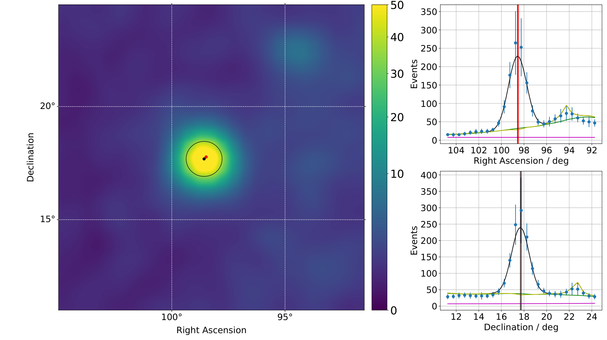
Figure 10 shows a AMS-02 conversion mode count map for a section of the sky centered on the Geminga pulsar in equatorial coordinates in the large plot on the left side. The smaller, right hand side, figures show projections onto the two axes. The 4FGL catalog position of the pulsar is indicated by the red dot in the center of the left figure and by red vertical lines in the right hand side projections.
The two dimensional distribution, shown in color, is fit with a background plus signal model, in which the background is held fixed and modeled by the predetermined background component (see section 7), the diffuse emission model and the sum of the fluxes of all sources in the window except Geminga. The signal model is a two-dimensional Gaussian with width determined by the energy dependent PSF of the conversion mode analysis. The mean values (the position) of the Gaussian and it’s normalization are left free in the fit.
The background (violet), diffuse emission (green), other sources (yellow) and total model (black) after the fit are shown in the one dimensional projections. Overall the model agrees very well with the measured data. The small bump in the yellow curve on the right hand side of the top right figure is the Supernova Remnant IC 443.
Resulting from the fit is the source position (), which agrees within uncertainties with the catalog position () [109]. This demonstrates that there is no significant bias in the pointing of the AMS detector or the reconstruction of the photon directions. The reconstructed position is indicated by the black dot in the two dimensional plot and by the vertical black lines in the projections.

The flux of the pulsar is obtained in a window, centered around the 4FGL position of Geminga, . The results from both AMS-02 and Fermi-LAT are shown in figure 11. The spectrum of Geminga is exponentially cut-off around . Above diffuse emission dominates the window flux.
The flux measured by AMS-02 agrees well with the Fermi-LAT flux measurement. In addition, it also agrees well with the model over the entire energy range.
The Geminga pulsar can also be identified by its pulsed emission of photons. The AMS-02 event timestamps are assigned by the main DAQ system of the experiment. The clock of the DAQ system is corrected for drift and synchronized with the GPS system of AMS on a daily basis. As a result the recorded events can be used for precision timing.
In order to correct for the light travel time as well as relativistic effects the photon arrival times must be converted from the TAI timescale to the TDB timescale 11 1 TAI (Temps Atomique International) is the International Atomic Time standard and TDB (Temps Dynamique Barycentrique) is Barycentric Dynamical Time, a time scale which includes relativistic corrections needed to convert times to equivalent instants in the Solar System barycenter., which can be done with appropriate software [139]. To account for the motion of the Earth and the ISS with respect to Geminga, the JPL DE430 planetary ephemerides [184] are used to calculate the exact position of the solar system barycenter and to convert the photon arrival times to the barycentric arrival times. This correction includes the Rømer delay for the orbital motion of the Earth and the Einstein and Shapiro delay to account for relativistic effects.
Pulsar ephemerides are required to account for the pulsar’s proper motion, it’s dispersion measure and to provide good estimates of its position and rotational parameters. Such ephemerides are available from the radio telescope community, for example from the Australia Telescope National Facility (ATNF)[185, 186]. Since Geminga is radio-quiet, a timing model from the Fermi-LAT FSSC[187, 188] is used here. In the used timing model the white noise of the pulsar’s timing is removed using a tabulated function.


Figure 12 shows the phase folded light curve of the Geminga pulsar, using all events (from both AMS-02 analysis modes) between and , in a window around the pulsar. Note that the same data is shown twice, which avoids the visual problem of wrapping events at the borders near phase 0 and 1. The left hand side shows the pre-fit result, using the pulsar ephemerides without modifications. For event times before 2015 the phaseogram is approximately constant, but the pulse begins to drift away after that point, which is a consequence of the fact that the model is being extrapolated.
In order to fix this problem the timing solution can be fitted, by using the TEMPO2 [189] and PINT [190] software packages. The result is shown on the right hand side of figure 12. This reveals a second peak in the pulse profile, approximately offset by half a pulsar rotation from the strongest peak. The curve in the phaseogram has disappeared and the pulse profile is clearly visible from the phase folded light curve. The fit solutions for the pulsar’s rotational period and spindown at the epoch (MJD 54800) are:
which places thne Geminga pulsar in the main population of pulsars in the diagram (see figure 19). The canonical age and surface magnetic field strength of the pulsar can be estimated using equations (15) and (14):
which constitutes a young to middle aged pulsar with a strong magnetic field.
The Crab and Vela Pulsars
In analogy to the flux from the Geminga region, figures 14 and 14 show the fluxes obtained in windows around the Crab and Vela pulsars. In the case of the Crab pulsar the agreement between AMS-02 and Fermi-LAT is excellent. At the highest energies the measured AMS-02 flux is incompatible with pure diffuse photon production, which is a result of the high energy inverse Comton component of the Crab PWN.
The measured flux in the Vela region is slightly lower than the Fermi-LAT result on average. Although it is not excluded that the Fermi measurement is slightly to high, the discrepancy could also be a result of the southern location of the source and its proximity to the southern exposure hole in both AMS analysis modes. The overall agreement of the flux shape is still good however, and the exponential cutoff is well reproduced.
The Flaring Blazar CTA-102
The Flat Spectrum Radio Quasar CTA-102 was discovered in the 1960s in the Caltech radio survey [191]. It is located at redshift [192] and was once proposed to be home to an extraterrestrial civilization, because of its variability in the radio band (this was before the discovery of pulsars, which were also associated with extraterrestrial life at first).


Figure 16 shows the measured flux for both AMS-02 and Fermi-LAT. The AMS flux is systematically slightly below the measured Fermi flux. However, both measured fluxes are significantly higher than the 4FGL catalog prediction. This is because the source is highly variable. The catalog was constructed based on data collected between August 2008 and August 2016 [109]. The AMS-02 flux, as well as the Fermi-LAT flux presented here, were derived from photon data collected between May 2011 and November 2017.
The blazar CTA-102 entered into a very active flaring state in the second half of 2016 [193], with multiple outburst in that period. The strongest flares were observed first in the middle of December 2016 and in particular in a period which started on December 28th 2016 and lasted for a few days. The flaring activity which began on December 28th was also registered by the AMS-02 detector.
Figure 16 shows the distribution of observed event counts in window around the CTA-102 source as a function of time. Each bin contains 3 days of collected data. The 12 days beginning on December 28th 2016 contain 25 events, which is the result of an enormous increase of flux. During December 2016 and January 2017 this source was measured to be the strongest -ray sources in the sky.
The source entered another period of strong flaring activity in April 2017. In this period, the flux was shown to be variable on timescales as short as 5 minutes, which leads to an estimation of the emission region which is smaller than the light travel time across the black hole at the center of the blazar ( light minutes) [194]. As a consequence, a compact emission region inside the jet itself was proposed.
Chapter 6 Summary
The AMS-02 measurement of -rays presented in this thesis is the first independent test of the Fermi-LAT data in the energy range from to .
The results show that the AMS-02 detector contributes valuable information to the measurement of high energy -rays in this energy range.
Two complementary analysis methods were developed and successfully applied to the AMS-02 data. The two measurements are almost entirely independent, because different parts of the experiment are used in their derivation.
The conversion mode analysis is suitable for photon energies between and . It features a very good angular resolution of at and improves with energy. The on-axis effective area is approximately for photon energy.
In the calorimeter analysis the pointing resolution is worse than in the conversion mode at low energies, but is still better than above . The energy resolution of the calorimeter is excellent and allows photon reconstruction up to energies. The peak on-axis effective area is .
A predictive model of the AMS-02 sky, including diffuse emission and -ray sources was developed and compared with the data, showing excellent agreement.
A dedicated Fermi-LAT analysis of high energy photons was carried out, which included a correction for the absolute energy scale shift of found by the LAT team.
The results for the -ray flux in the inner galaxy (), which is dominated by diffuse emission, show that two AMS-02 analysis modes are in excellent agreement, which excludes sizable systematic uncertainties.
The results are also in good agreement with the measured Fermi-LAT flux, if the absolute energy scale correction is applied to the LAT data. In case it is not applied the disagreement is at the level of 6.8 standard deviations, which shows that the energy scale correction must be considered in the LAT photon analysis. This new result highlights the importance of the AMS-02 measurement.
The measured emission from the Cygnus-X is also in good agreement with the LAT data. The high energy fluxes of the pulsars Geminga, Crab and Vela were presented. In all cases the AMS-02 results are in excellent agreement with the Fermi-LAT result. A pulsar timing analysis for Geminga was presented, which allowed to determine the pulsar’s period of rotation and its spindown with excellent precision.
Finally AMS-02 observed the outburst of a flaring blazar, CTA-102, whose measured flux is also in agreement with the Fermi-LAT result.
References
- [1] Aguilar, M., et al. Electron and Positron Fluxes in Primary Cosmic Rays Measured with the Alpha Magnetic Spectrometer on the International Space Station. Phys. Rev. Lett., Volume 113:121102 [2014].
- [2] Aguilar, M., et al. Observation of Complex Time Structures in the Cosmic-Ray Electron and Positron Fluxes with the Alpha Magnetic Spectrometer on the International Space Station. Phys. Rev. Lett., Volume 121:051102 [2018].
- [3] Räihä, T., et al. Monte Carlo simulations of the transition radiation detector of the AMS-02 experiment. Nuclear Instruments and Methods in Physics Research Section A: Accelerators, Spectrometers, Detectors and Associated Equipment, Volume 868:10 – 14 [2017].
- [4] Aguilar, M., et al. First Result from the Alpha Magnetic Spectrometer on the International Space Station: Precision Measurement of the Positron Fraction in Primary Cosmic Rays of 0.5–350 GeV. Phys. Rev. Lett., Volume 110:141102 [2013].
- [5] Accardo, L., et al. High Statistics Measurement of the Positron Fraction in Primary Cosmic Rays of 0.5–500 GeV with the Alpha Magnetic Spectrometer on the International Space Station. Phys. Rev. Lett., Volume 113:121101 [2014].
- [6] Aguilar, M., et al. Precision Measurement of the Flux in Primary Cosmic Rays from 0.5 GeV to 1 TeV with the Alpha Magnetic Spectrometer on the International Space Station. Phys. Rev. Lett., Volume 113:221102 [2014].
- [7] Aguilar, M., et al. Precision Measurement of the Proton Flux in Primary Cosmic Rays from Rigidity 1 GV to 1.8 TV with the Alpha Magnetic Spectrometer on the International Space Station. Phys. Rev. Lett., Volume 114:171103 [2015].
- [8] Aguilar, M., et al. Precision Measurement of the Helium Flux in Primary Cosmic Rays of Rigidities 1.9 GV to 3 TV with the Alpha Magnetic Spectrometer on the International Space Station. Phys. Rev. Lett., Volume 115:211101 [2015].
- [9] Aguilar, M., et al. Antiproton Flux, Antiproton-to-Proton Flux Ratio, and Properties of Elementary Particle Fluxes in Primary Cosmic Rays Measured with the Alpha Magnetic Spectrometer on the International Space Station. Phys. Rev. Lett., Volume 117:091103 [2016].
- [10] Aguilar, M., et al. Precision Measurement of the Boron to Carbon Flux Ratio in Cosmic Rays from 1.9 GV to 2.6 TV with the Alpha Magnetic Spectrometer on the International Space Station. Phys. Rev. Lett., Volume 117:231102 [2016].
- [11] Aguilar, M., et al. Observation of the Identical Rigidity Dependence of He, C, and O Cosmic Rays at High Rigidities by the Alpha Magnetic Spectrometer on the International Space Station. Phys. Rev. Lett., Volume 119:251101 [2017].
- [12] Aguilar, M., et al. Observation of New Properties of Secondary Cosmic Rays Lithium, Beryllium, and Boron by the Alpha Magnetic Spectrometer on the International Space Station. Phys. Rev. Lett., Volume 120:021101 [2018].
- [13] Aguilar, M., et al. Precision Measurement of Cosmic-Ray Nitrogen and its Primary and Secondary Components with the Alpha Magnetic Spectrometer on the International Space Station. Phys. Rev. Lett., Volume 121:051103 [2018].
- [14] Aguilar, M., et al. Observation of Fine Time Structures in the Cosmic Proton and Helium Fluxes with the Alpha Magnetic Spectrometer on the International Space Station. Phys. Rev. Lett., Volume 121:051101 [2018].
- [15] Aguilar, M., et al. Towards Understanding the Origin of Cosmic-Ray Positrons. Phys. Rev. Lett., Volume 122:041102 [2019].
- [16] Aguilar, M., et al. Towards Understanding the Origin of Cosmic-Ray Electrons. Phys. Rev. Lett., Volume 122:101101 [2019].
- [17] Aguilar, M., et al. Properties of Cosmic Helium Isotopes Measured by the Alpha Magnetic Spectrometer. Phys. Rev. Lett., Volume 123:181102 [2019].
- [18] Dodelson, S., et al. Constraining cosmological dark matter annihilation with gamma ray observations. Phys. Rev. D, Volume 80(8):083504–9 [2009].
- [19] Serpico, P. D. et al. Gamma rays from dark matter annihilation in the central region of the Galaxy. New Journal of Physics, Volume 11(10):105010 [2009].
- [20] Bringmann, T. et al. Gamma ray signals from dark matter: Concepts, status and prospects. Physics of the Dark Universe, Volume 1(1):194 – 217 [2012]. Next Decade in Dark Matter and Dark Energy.
- [21] Ackermann, M., et al. Searching for Dark Matter Annihilation from Milky Way Dwarf Spheroidal Galaxies with Six Years of Fermi Large Area Telescope Data. Phys. Rev. Lett., Volume 115(23):231301 [2015].
- [22] Ackermann, M., et al. Constraining Dark Matter Models from a Combined Analysis of Milky Way Satellites with the Fermi Large Area Telescope. Phys. Rev. Lett., Volume 107(24):241302 [2011].
- [23] Ackermann, M., et al. Fermi-LAT Observations of the Diffuse -Ray Emission: Implications for Cosmic Rays and the Interstellar Medium. The Astrophysical Journal, Volume 750(1):3 [2012].
- [24] Acero, F., et al. Development of the Model of Galactic Interstellar Emission for Standard Point-source Analysis of Fermi Large Area Telescope Data. The Astrophysical Journal Supplement Series, Volume 223(2):26 [2016].
- [25] Hooper, D. et al. Dark matter annihilation in the Galactic Center as seen by the Fermi Gamma Ray Space Telescope. Physics Letters B, Volume 697(5):412–428 [2011].
- [26] Daylan, T., et al. The characterization of the gamma-ray signal from the central Milky Way: A case for annihilating dark matter. Physics of the Dark Universe, Volume 12:1–23 [2016].
- [27] Ackermann, M., et al. The Fermi Galactic Center GeV Excess and Implications for Dark Matter. The Astrophysical Journal, Volume 840(1):43 [2017].
- [28] Su, M., et al. Giant Gamma-ray Bubbles from Fermi-LAT: Active Galactic Nucleus Activity or Bipolar Galactic Wind? ApJ, Volume 724(2):1044–1082 [2010].
- [29] Abbott, B. P., et al. GW170817: Observation of Gravitational Waves from a Binary Neutron Star Inspiral. Phys. Rev. Lett., Volume 119(16):161101 [2017].
- [30] IceCube Collaboration, et al. Multimessenger observations of a flaring blazar coincident with high-energy neutrino IceCube-170922A. Science, Volume 361(6398):eaat1378 [2018].
- [31] Kraushaar, W. L., et al. High-Energy Cosmic Gamma-Ray Observations from the OSO-3 Satellite. ApJ, Volume 177:341 [1972].
- [32] Fichtel, C. E., et al. High-energy gamma-ray results from the second Small Astronomy Satellite. ApJ, Volume 198:163–182 [1975].
- [33] Bignami, G. F., et al. The COS-B experiment for gamma-ray astronomy. Space Science Instrumentation, Volume 1:245–268 [1975].
- [34] Hartman, R. C., et al. The EGRET High Energy Gamma Ray Telescope. In NASA Conference Publication, Volume 3137 of NASA Conference Publication, pages 116–125 [1992].
- [35] Hartman, R. C., et al. The Third EGRET Catalog of High-Energy Gamma-Ray Sources. ApJS, Volume 123(1):79–202 [1999].
- [36] Hunter, S. D., et al. EGRET Observations of the Diffuse Gamma-Ray Emission from the Galactic Plane. ApJ, Volume 481(1):205–240 [1997].
- [37] Meegan, C. A., et al. Spatial distribution of -ray bursts observed by BATSE. Nature, Volume 355(6356):143–145 [1992].
- [38] Schoenfelder, V., et al. Instrument Description and Performance of the Imaging Gamma-Ray Telescope COMPTEL aboard the Compton Gamma-Ray Observatory. ApJS, Volume 86:657 [1993].
- [39] Atwood, W. B. et al. The Large Area Telescope on the Fermi Gamma-ray Space Telescope Mission [2009].
- [40] Meegan, C., et al. The Fermi Gamma-ray Burst Monitor. ApJ, Volume 702(1):791–804 [2009].
- [41] Ferenc, D. et al. The MAGIC gamma-ray observatory. Nuclear Instruments and Methods in Physics Research A, Volume 553(1-2):274–281 [2005].
- [42] Hinton, J. A. et al. The status of the HESS project. New A Rev., Volume 48(5-6):331–337 [2004].
- [43] Weekes, T. C., et al. VERITAS: the Very Energetic Radiation Imaging Telescope Array System. Astroparticle Physics, Volume 17(2):221–243 [2002].
- [44] Actis, M., et al. Design concepts for the Cherenkov Telescope Array CTA: an advanced facility for ground-based high-energy gamma-ray astronomy. Experimental Astronomy, Volume 32(3):193–316 [2011].
- [45] Atwood, W. B., et al. The Large Area Telescope on the Fermi Gamma-Ray Space Telescope Mission. The Astrophysical Journal, Volume 697(2):1071 [2009].
- [46] Kounine, A., et al. Precision measurement of 0.5 GeV - 3 TeV electrons and positrons using the AMS Electromagnetic Calorimeter. Nuclear Instruments and Methods in Physics Research Section A: Accelerators, Spectrometers, Detectors and Associated Equipment, Volume 869:110 – 117 [2017].
- [47] Adloff, C., et al. The AMS-02 lead-scintillating fibres Electromagnetic Calorimeter. Nuclear Instruments and Methods in Physics Research Section A: Accelerators, Spectrometers, Detectors and Associated Equipment, Volume 714:147 – 154 [2013].
- [48] Ackermann, M., et al. In-flight measurement of the absolute energy scale of the Fermi Large Area Telescope. Astroparticle Physics, Volume 35(6):346 – 353 [2012].
- [49] Abdollahi, S., et al. Cosmic-ray electron-positron spectrum from 7 GeV to 2 TeV with the Fermi Large Area Telescope. Phys. Rev. D, Volume 95:082007 [2017].
- [50] Ackermann, M., et al. Detection of the Characteristic Pion-Decay Signature in Supernova Remnants. Science, Volume 339(6121):807–811 [2013].
- [51] Tsai, Y.-S. Pair production and bremsstrahlung of charged leptons. Rev. Mod. Phys., Volume 46:815–851 [1974].
- [52] Landau, L. D. et al. Limits of applicability of the theory of bremsstrahlung electrons and pair production at high-energies. Dokl. Akad. Nauk Ser. Fiz., Volume 92:535 [1953].
- [53] Migdal, A. B. Bremsstrahlung and Pair Production in Condensed Media at High Energies. Phys. Rev., Volume 103:1811–1820 [1956].
- [54] Tanabashi, M., et al. Review of Particle Physics. Phys. Rev. D, Volume 98:030001 [2018].
- [55] Klein, O. et al. Über die Streuung von Strahlung durch freie Elektronen nach der neuen relativistischen Quantendynamik von Dirac. Zeitschrift für Physik, Volume 52(11):853–868 [1929].
- [56] Cheng, K. S. et al. The Synchrotron Self-Compton Model for X-Ray and gamma -Ray Emission from Pulsars. ApJ, Volume 448:281 [1995].
- [57] Jóhannesson, G., et al. The Three-dimensional Spatial Distribution of Interstellar Gas in the Milky Way: Implications for Cosmic Rays and High-energy Gamma-ray Emissions. The Astrophysical Journal, Volume 856(1):45 [2018].
- [58] Aguilar, M. et al. Cosmic-ray positron fraction measurement from 1-GeV to 30- GeV with AMS-01. Phys. Lett., Volume B646:145–154 [2007].
- [59] Adriani, O. et al. An anomalous positron abundance in cosmic rays with energies 1.5.100 GeV. Nature, Volume 458:607–609 [2009].
- [60] Hooper, D., et al. Excesses in cosmic ray positron and electron spectra from a nearby clump of neutralino dark matter. Phys. Rev. D., Volume 79:103513 [2009].
- [61] Hooper, D., et al. Pulsars as the sources of high energy cosmic ray positrons. Journal of Cosmology and Astroparticle Physics, Volume 2009(01):025 [2009].
- [62] Pierre Auger Collaboration. The Pierre Auger Cosmic Ray Observatory. Nuclear Instruments and Methods in Physics Research A, Volume 798:172–213 [2015].
- [63] Adriani, O., et al. PAMELA Measurements of Cosmic-Ray Proton and Helium Spectra. Science, Volume 332(6025):69–72 [2011].
- [64] Chang, J., et al. The DArk Matter Particle Explorer mission. Astroparticle Physics, Volume 95:6–24 [2017].
- [65] D. A. M. P. E. Collaboration, et al. Measurement of the cosmic ray proton spectrum from 40 GeV to 100 TeV with the DAMPE satellite. Science Advances, Volume 5(9) [2019].
- [66] Strong, A. W. et al. Propagation of Cosmic-Ray Nucleons in the Galaxy. The Astrophysical Journal, Volume 509(1):212–228 [1998].
- [67] Strong, A. W., et al. The GALPROP code for cosmic-ray transport and diffuse emission production., https://galprop.stanford.edu.
- [68] Torii, S. et al. Calorimetric electron telescope mission. Search for dark matter and nearby sources. Nuclear Instruments and Methods in Physics Research A, Volume 630(1):55–57 [2011].
- [69] Adriani, O., et al. Energy Spectrum of Cosmic-Ray Electron and Positron from 10 GeV to 3 TeV Observed with the Calorimetric Electron Telescope on the International Space Station. Phys. Rev. Lett., Volume 119:181101 [2017].
- [70] Aharonian, F., et al. Probing the ATIC peak in the cosmic-ray electron spectrum with H.E.S.S. Astronomy and Astrophysics, Volume 508(2):561–564 [2009].
- [71] Aharonian, F., et al. Energy Spectrum of Cosmic-Ray Electrons at TeV Energies. Phys. Rev. Lett., Volume 101(26):261104 [2008].
- [72] D. A. M. P. E. Collaboration, et al. Direct detection of a break in the teraelectronvolt cosmic-ray spectrum of electrons and positrons. Nature, Volume 552:63 [2017].
- [73] S. W. Barwick, e. a. Measurements of the Cosmic-Ray Positron Fraction from 1 to 50 GeV. The Astrophysical Journal Letters, Volume 482(2):L191– [1997].
- [74] Cirelli, M. et al. Minimal Dark Matter predictions and the PAMELA positron excess [2008].
- [75] Chowdhury, D., et al. Results from PAMELA, ATIC and FERMI : Pulsars or Dark Matter ? [2009].
- [76] Ando, S., et al. Dark matter annihilation or unresolved astrophysical sources? Anisotropy probe of the origin of cosmic gamma-ray background. Phys. Rev., Volume D75:063519 [2007].
- [77] Kalberla, P. M. W., et al. The Leiden/Argentine/Bonn (LAB) Survey of Galactic HI - Final data release of the combined LDS and IAR surveys with improved stray-radiation corrections. A&A, Volume 440(2):775–782 [2005].
- [78] HI4PI Collaboration:, et al. HI4PI: a full-sky H I survey based on EBHIS and GASS. A&A, Volume 594:A116 [2016].
- [79] Sofue, Y. Dark halos of M 31 and the Milky Way. Publications of the Astronomical Society of Japan, Volume 67(4) [2015].
- [80] He, C., et al. The Correlation between Dispersion Measure and X-Ray Column Density from Radio Pulsars. The Astrophysical Journal, Volume 768(1):64 [2013].
- [81] Freudenreich, H. T. A COBE Model of the Galactic Bar and Disk. The Astrophysical Journal, Volume 492(2):495–510 [1998].
- [82] Porter, T. A., et al. High-energy Gamma Rays from the Milky Way: Three-dimensional Spatial Models for the Cosmic-Ray and Radiation Field Densities in the Interstellar Medium. The Astrophysical Journal, Volume 846(1):67 [2017].
- [83] Robitaille, T.P., et al. A self-consistent model of Galactic stellar and dust infrared emission and the abundance of polycyclic aromatic hydrocarbons. A&A, Volume 545:A39 [2012].
- [84] Sodroski, T. J., et al. A Three-dimensional Decomposition of the Infrared Emission from Dust in the Milky Way. The Astrophysical Journal, Volume 480(1):173–187 [1997].
- [85] Miville-Deschenes, M.-A. et al. IRIS: A New Generation of IRAS Maps. The Astrophysical Journal Supplement Series, Volume 157(2):302–323 [2005].
- [86] Fazio, G. G., et al. The Infrared Array Camera (IRAC) for theSpitzer Space Telescope. The Astrophysical Journal Supplement Series, Volume 154(1):10–17 [2004].
- [87] Aeronautics, N. et al. A Giant Hubble Mosaic of the Crab Nebula [2005], https://hubblesite.org/contents/media/images/2005/37/1823-Image.html.
- [88] Shklovskii, I. S. On the Nature of the Optical Emission from the Crab Nebula. Soviet Ast., Volume 1:690 [1957].
- [89] Chandrasekhar, S. The Maximum Mass of Ideal White Dwarfs. ApJ, Volume 74:81 [1931].
- [90] Tolman, R. C. Static Solutions of Einstein’s Field Equations for Spheres of Fluid. Physical Review, Volume 55(4):364–373 [1939].
- [91] Oppenheimer, J. R. et al. On Massive Neutron Cores. Physical Review, Volume 55(4):374–381 [1939].
- [92] Wikipedia. Schematic view of a pulsar [2007], https://commons.wikimedia.org/wiki/File:Pulsar_schematic.svg.
- [93] Aeronautics, N. et al. Combined X-Ray and Optical Images of the Crab Nebula [2002], https://hubblesite.org/contents/media/images/2002/24/1248-Image.html.
- [94] Harding, A. K. Gamma-ray Pulsars: Models and Predictions. AIP Conference Proceedings, Volume 558(1):115–126 [2001].
- [95] Condon, J. J. et al. Essential Radio Astronomy [2016].
- [96] Condon, James and Ransom, Scott. Essential Radio Astronomy, https://www.cv.nrao.edu/˜sransom/web/Ch6.html.
- [97] Drake, F. D. Radio Observations of the Crab Nebula Pulsar. In Davies, R. D. et al., editors, The Crab Nebula, Volume 46 of IAU Symposium, page 73 [1971].
- [98] Mattox, J. R., et al. SAS 2 Observation of Pulsed High-Energy Gamma Radiation from Geminga. ApJ, Volume 401:L23 [1992].
- [99] Abdo, A. A., et al. Fermi-LAT Observations of the Geminga Pulsar. The Astrophysical Journal, Volume 720(1):272 [2010].
- [100] McLaughlin, M. A. The North American Nanohertz Observatory for Gravitational Waves. Classical and Quantum Gravity, Volume 30(22):224008 [2013].
- [101] Anderson, P. W. et al. Pulsar glitches and restlessness as a hard superfluidity phenomenon. Nature, Volume 256(5512):25–27 [1975].
- [102] Australia Telescope National Facility. ATNF Glitch Database, https://www.atnf.csiro.au/research/pulsar/psrcat/glitchTbl.html.
- [103] Urry, C. M. et al. Unified Schemes for Radio-Loud Active Galactic Nuclei. PASP, Volume 107:803 [1995].
- [104] Aeronautics, N. et al. A Multi-Wavelength View of the Radio Galaxy Hercules A [2012], https://hubblesite.org/contents/media/images/2012/47/3110-Image.html.
- [105] Beckmann, V. et al. The AGN phenomenon: open issues. In Proceedings of “An INTEGRAL view of the high-energy sky (the first 10 years)” - 9th INTEGRAL Workshop and celebration of the 10th anniversary of the launch (INTEGRAL 2012). 15-19 October 2012. Bibliotheque Nationale de France, page 69 [2012].
- [106] Abdo, A. A., et al. Fermi Large Area Telescope Observations of Markarian 421: The Missing Piece of its Spectral Energy Distribution. The Astrophysical Journal, Volume 736(2):131 [2011].
- [107] Konopelko, A., et al. Modeling the TeV Gamma-Ray Spectra of Two Low-Redshift Active Galactic Nuclei: Markarian 501 and Markarian 421. The Astrophysical Journal, Volume 597(2):851–859 [2003].
- [108] Su, M., et al. Giant Gamma-Ray Bubbles from Fermi-LAT: Active Galactic Nucleus Activity or Bipolar Galactic Wind? The Astrophysical Journal, Volume 724(2):1044–1082 [2010].
- [109] The Fermi-LAT collaboration. Fermi Large Area Telescope Fourth Source Catalog. arXiv e-prints, arXiv:1902.10045 [2019].
- [110] The Fermi-LAT collaboration. Galactic Interstellar Emission Model for the 4FGL Catalog Analysis, https://fermi.gsfc.nasa.gov/ssc/data/analysis/software/aux/4fgl/Galactic_Diffuse_Emission_Model_for_the_4FGL_Catalog_Analysis.pdf.
- [111] Ackermann, M., et al. The Spectrum of Isotropic Diffuse Gamma-Ray Emission between 100 MeV and 820 GeV. ApJ, Volume 799(1):86 [2015].
- [112] Acero, F., et al. Fermi Large Area Telescope Third Source Catalog. The Astrophysical Journal Supplement Series, Volume 218(2):23 [2015].
- [113] National Aeronautics and Space Administration. International Space Station Gallery, https://www.nasa.gov/mission_pages/station/images/station_post_construction/index.html.
- [114] Kounine, A. The Alpha Magnetic Spectrometer on the International Space Station. International Journal of Modern Physics E, Volume 21(08):1230005 [2012].
- [115] NASA. Visible Earth [2002], https://visibleearth.nasa.gov/view.php?id=57730.
- [116] National Aeronautics and Space Administration. The International Space Station’s coordinate system, https://www.nasa.gov/mission_pages/station/multimedia/iss_labs_guide.html.
- [117] National Aeronautics and Space Administration. Space Station Reference Coordinate Systems, https://pims.grc.nasa.gov/plots/user/tibor/SSP30219JISSCoordSystems.pdf.
- [118] Vondrák, J. et al. International Earth Rotation and Reference Systems Service (IERS) web: www.iers.org. Journal of Geodesy, Volume 77(10-11):585–678 [2004].
- [119] Petit, G. et al. IERS Conventions (2010). Verlag des Bundesamts für Kartographie und Geodäsie [2010].
- [120] Altamimi, Z., et al. ITRF2014: A new release of the International Terrestrial Reference Frame modeling nonlinear station motions. Journal of Geophysical Research: Solid Earth, Volume 121(8):6109–6131 [2016].
- [121] National Geospatial-Intelligence Agency - Office of Geomagnetics. Department of Defense (DoD) World Geodetic System (WGS) 1984 - Its Definition and Relationships with Local Geodetic Systems [2014].
- [122] Wikipedia. RA and Dec on celestial sphere [2012], https://en.wikipedia.org/wiki/File:Ra_and_dec_on_celestial_sphere.png.
- [123] Aeronautics, N. et al. General Mission Analysis Tool [2012], http://gmat.sourceforge.net/docs/nightly/files/images/Resource_CoordinateSystems_GUI_5.png.
- [124] Kaplan, G. The IAU Resolutions on Astronomical Reference Systems, Time Scales, and Earth Rotation Models: Explanation and Implementation. United States Naval Observatory Circular 179 [2005].
- [125] International Astronomical Union. IAU 1976 Resolution 1 [1976].
- [126] Fricke, W., et al. Fourth Fundamental Catalogue (FK4). Veröffentlichungen des Astronomischen Rechen-Instituts Heidelberg, Volume 10:1–144 [1963].
- [127] Fricke, W., et al. Fifth Fundamental Catalogue (FK5). Part 1. The Basic Fundamental Stars. Veröffentlichungen des Astronomischen Rechen-Instituts Heidelberg, Volume 32:1–106 [1988].
- [128] Perryman, M. A. C., et al. The Hipparcos Catalogue. Astronomy and Astrophysics, Volume 500:501–504 [1997].
- [129] Wielen, R., et al. Sixth Catalogue of Fundamental Stars (FK6). Part I. Basic fundamental stars with direct solutions. Veröffentlichungen des Astronomischen Rechen-Instituts Heidelberg, Volume 35 [1999].
- [130] Arias, E. F., et al. The extragalactic reference system of the International Earth Rotation Service, ICRS. Astronomy and Astrophysics, Volume 303:604–608 [1995].
- [131] Ma, C., et al. The International Celestial Reference Frame as Realized by Very Long Baseline Interferometry. The Astronomical Journal, Volume 116(1):516–546 [1998].
- [132] International Astronomical Union. IAU 1997 Resolution B2 [1997].
- [133] Mignard, F. et al. Linking the FK5 to the ICRF. Highlights of Astronomy, Volume 11:313 [1998].
- [134] Observatory, E. S. Artist’s impression of the Milky Way [2013], https://www.eso.org/public/images/eso1339e.
- [135] Blaauw, A., et al. The New I.A.U. System of Galactic Coordinates (1958 Revision). Monthly Notices of the Royal Astronomical Society, Volume 121(2):123–131 [1960].
- [136] Murray, C. A. The transformation of coordinates between the system of B1950.0 and J2000.0, and the principal galactic axes referred to J2000.0. Astronomy and Astrophysics, Volume 218:325–329 [1989].
- [137] Liu, J.-C., et al. Reconsidering the Galactic coordinate system. Astronomy & Astrophysics, Volume 526:A16 [2011].
- [138] Reid, M. J. et al. The Proper Motion of Sagittarius A*. II. The Mass of Sagittarius A*. The Astrophysical Journal, Volume 616(2):872–884 [2004].
- [139] The Astropy Collaboration, et al. The Astropy Project: Building an Open-science Project and Status of the v2.0 Core Package. The Astronomical Journal, Volume 156:123 [2018].
- [140] Vallado, D., et al. Revisiting Spacetrack Report #3. AIAA/AAS Astrodynamics Specialist Conference [2006].
- [141] Hoots, F. et al. Spacetrack Report No. 3 - Models for Propagation of NORAD Element Sets. United States Air Force Aerospace Defense Command [1980].
- [142] Magliacane, J. A. PREDICT: Satellite tracking and orbital prediction [2011].
- [143] Capitaine, N., et al. Definition of the Celestial Ephemeris Origin and of UT1 in the International Celestial Reference Frame. Astronomy and Astrophysics, Volume 355:398–405 [2000].
- [144] International Astronomical Union. IAU 2000 Resolution B1.8 [2000].
- [145] Capitaine, N., et al. Expressions for IAU 2000 precession quantities. Astronomy and Astrophysics, Volume 412(2):567–586 [2003].
- [146] International Astronomical Union. IAU 2000 Resolution B1.3 [2000].
- [147] International Astronomical Union. IAU 2000 Resolution B1.6 [2000].
- [148] Mathews, P. M., et al. Modeling of nutation and precession: New nutation series for nonrigid Earth and insights into the Earth’s interior. Journal of Geophysical Research: Solid Earth, Volume 107(B4):ETG 3–1–ETG 3–26 [2002].
- [149] International Astronomical Union. IAU 2006 Resolution B1 [2006].
- [150] Hilton, J. L., et al. Report of the International Astronomical Union Division I Working Group on Precession and the Ecliptic. Celestial Mechanics and Dynamical Astronomy, Volume 94(3):351–367 [2006].
- [151] Lieske, J. H., et al. Expressions for the Precession Quantities Based upon the IAU (1976) System of Astronomical Constants. Astronomy and Astrophysics, Volume 58:1–16 [1977].
- [152] Seidelmann, P. K. 1980 I.A.U. Theory of Nutation - the Final Report of the I.A.U. Working Group on Nutation. Celestial Mechanics, Volume 27(1):79–106 [1982].
- [153] IAU SOFA Board. IAU SOFA Software Collection [2019], http://www.iausofa.org.
- [154] AMS Collaboration. Alpha Magnetic Spectrometer Website, https://ams02.space.
- [155] Lübelsmeyer, K., et al. Upgrade of the Alpha Magnetic Spectrometer (AMS-02) for long term operation on the International Space Station (ISS). Nuclear Instruments and Methods in Physics Research Section A: Accelerators, Spectrometers, Detectors and Associated Equipment, Volume 654(1):639 – 648 [2011].
- [156] Berdugo, J., et al. Determination of the rigidity scale of the Alpha Magnetic Spectrometer. Nuclear Instruments and Methods in Physics Research Section A: Accelerators, Spectrometers, Detectors and Associated Equipment, Volume 869:10 – 14 [2017].
- [157] University of Geneva. AMS Tracker Integration and Assembly Pictures, http://dpnc.unige.ch/ams/ams_beta/Welcome_New.shtml.
- [158] Azzarello, P. Tests and production of the AMS-02 silicon tracker detectors. Ph.D. thesis, Geneva U. [2004].
- [159] Ambrosi, G., et al. The spatial resolution of the silicon tracker of the Alpha Magnetic Spectrometer. Nuclear Instruments and Methods in Physics Research Section A: Accelerators, Spectrometers, Detectors and Associated Equipment, Volume 869:29 – 37 [2017].
- [160] Bindi, V., et al. Calibration and performance of the AMS-02 time of flight detector in space. Nuclear Instruments and Methods in Physics Research Section A: Accelerators, Spectrometers, Detectors and Associated Equipment, Volume 743:22 – 29 [2014].
- [161] Bindi, V., et al. The scintillator detector for the fast trigger and time-of-flight (TOF) measurement of the space experiment AMS-02. Nuclear Instruments and Methods in Physics Research Section A: Accelerators, Spectrometers, Detectors and Associated Equipment, Volume 623(3):968 – 981 [2010].
- [162] von Doetinchem, P., et al. The AMS-02 Anticoincidence Counter. Nuclear Physics B - Proceedings Supplements, Volume 197(1):15 – 18 [2009]. 11th Topical Seminar on Innovative Particle and Radiation Detectors (IPRD08).
- [163] Goerres, A. Kalibration und Integration des AMS-02 Anti-Koinzidenz-Detektors. Diplomarbeit, RWTH Aachen [2010].
- [164] RWTH Aachen. AMS TRD Website, https://www1b.physik.rwth-aachen.de/˜schael/AMS_TRD.html.
- [165] Schael, Stefan. First six years of AMS on the ISS and future perspectives, https://www1b.physik.rwth-aachen.de/˜schael/AMS-100_files/2018_04_23_MPI.pdf.
- [166] Li, Z.-Y., et al. Antiproton identification below threshold with the AMS-02 RICH detector. Chinese Physics C, Volume 41(5):056001 [2017].
- [167] Giovacchini, F. Performance in space of the AMS-02 RICH detector. Nuclear Instruments and Methods in Physics Research Section A: Accelerators, Spectrometers, Detectors and Associated Equipment, Volume 766:57 – 60 [2014]. RICH2013 Proceedings of the Eighth International Workshop on Ring Imaging Cherenkov Detectors Shonan, Kanagawa, Japan, December 2-6, 2013.
- [168] Brun, R. et al. ROOT - An object oriented data analysis framework. Nuclear Instruments and Methods in Physics Research Section A: Accelerators, Spectrometers, Detectors and Associated Equipment, Volume 389(1):81 – 86 [1997].
- [169] Agostinelli, S., et al. Geant4–a simulation toolkit. Nuclear Instruments and Methods in Physics Research Section A: Accelerators, Spectrometers, Detectors and Associated Equipment, Volume 506(3):250–303 [2003].
- [170] Qu, Z., et al. New track finding based on cellar automaton for AMS-02 detector. Nuclear Instruments and Methods in Physics Research Section A: Accelerators, Spectrometers, Detectors and Associated Equipment, Volume 869:135 – 140 [2017].
- [171] Fermi-LAT. Fermi-LAT Performance [2016], http://www.slac.stanford.edu/exp/glast/groups/canda/lat_Performance.htm.
- [172] Sullivan, J. D. Geometrical factor and directional response of single and multi-element particle telescopes. Nuclear Instruments and Methods, Volume 95:5 [1971].
- [173] Hoecker, A., et al. TMVA: Toolkit for Multivariate Data Analysis. PoS, Volume ACAT:040 [2007].
- [174] D’Agostini, G. A multidimensional unfolding method based on Bayes’ theorem. Nuclear Instruments and Methods in Physics Research Section A: Accelerators, Spectrometers, Detectors and Associated Equipment, Volume 362(2):487 – 498 [1995].
- [175] Zimmermann, N. Precision measurement of the cosmic-ray electron and positron fluxes as a function of time and energy with the Alpha Magnetic Spectrometer on the International Space Station. Ph.D. thesis, RWTH Aachen University [2019].
- [176] Atwood, W., et al. Pass 8: Toward the Full Realization of the Fermi-LAT Scientific Potential. arXiv e-prints, arXiv:1303.3514 [2013].
- [177] Bruel, P., et al. Fermi-LAT improved Pass 8 event selection. arXiv e-prints, arXiv:1810.11394 [2018].
- [178] Ackermann, M., et al. The Fermi Large Area Telescope On Orbit: Event Classification, Instrument Response Functions, and Calibration. The Astrophysical Journal Supplement Series, Volume 203(1):4 [2012].
- [179] Górski, K. M., et al. HEALPix: A Framework for High-Resolution Discretization and Fast Analysis of Data Distributed on the Sphere. Astrophys. J., Volume 622:759–771 [2005].
- [180] Lafferty, G. et al. Where to stick your data points: The treatment of measurements within wide bins. Nuclear Instruments and Methods in Physics Research Section A: Accelerators, Spectrometers, Detectors and Associated Equipment, Volume 355(2):541 – 547 [1995].
- [181] Caraveo, P. A., et al. Parallax Observations with the Hubble Space Telescope Yield the Distance to Geminga. The Astrophysical Journal, Volume 461(2) [1996].
- [182] Yuksel, H., et al. TeV Gamma Rays from Geminga and the Origin of the GeV Positron Excess. Phys. Rev. Lett., Volume 103:051101 [2009].
- [183] Abeysekara, A. U., et al. Extended gamma-ray sources around pulsars constrain the origin of the positron flux at Earth. Science, Volume 358(6365):911–914 [2017].
- [184] Jet Propulsion Laboratory. Solar System Dynamics - Ephemerides, https://ssd.jpl.nasa.gov/?ephemerides.
- [185] Manchester, R. N., et al. The Australia Telescope National Facility Pulsar Catalogue. The Astronomical Journal, Volume 129(4):1993–2006 [2005].
- [186] Australia Telescope National Facility. ATNF Pulsar Catalogue, https://www.atnf.csiro.au/research/pulsar/psrcat.
- [187] The Fermi-LAT collaboration. LAT Gamma-ray Pulsar Timing Models, https://confluence.slac.stanford.edu/display/GLAMCOG/LAT+Gamma-ray+Pulsar+Timing+Models.
- [188] Ray, P. S., et al. Precise -ray Timing and Radio Observations of 17 Fermi -ray pulsars. The Astrophysical Journal Supplement Series, Volume 194(2):17 [2011].
- [189] Hobbs, G. B., et al. TEMPO2, a new pulsar-timing package - I. An overview. Monthly Notices of the Royal Astronomical Society, Volume 369(2):655–672 [2006].
- [190] Luo, J., et al. PINT: High-precision pulsar timing analysis package [2019].
- [191] Harris, D. E. et al. Radio Source Measurements at 960 Mc/s. Publications of the Astronomical Society of the Pacific, Volume 72:237 [1960].
- [192] Monroe, T. R., et al. The UV-Bright Quasar Survey (UVQS): DR 1. The Astronomical Journal, Volume 152(1):25 [2016].
- [193] Prince, R., et al. Fermi-Large Area Telescope Observations of the Brightest Gamma-Ray Flare Ever Detected from CTA 102. The Astrophysical Journal, Volume 866(1):16 [2018].
- [194] Shukla, A., et al. Short-timescale -Ray Variability in CTA 102. The Astrophysical Journal, Volume 854(2):L26 [2018].
Appendix A TRD Pileup Study Electron Selection
In order to select electrons which enter the calorimeter from below and are fully absorbed there for the TRD pileup study in section 4 the following cuts are used:
- •
Positive physics trigger from the calorimeter.
- •
Exactly one reconstructed ECAL shower.
- •
Up-going longitudinal shower shape from a longitudinal shower fit.
- •
Angle between shower axis determination methods using the shower center of gravity in each layer and using ratios of cell amplitudes smaller than .
- •
No significant leakage of the shower to any side
- •
Ratio of energy release within around the shower core > 0.8.
- •
Ratio of energy release within around the shower core > 0.95.
- •
At most 1 lower TOF cluster.
- •
Deposited energy in each lower TOF layer smaller than .
open=any
Appendix B ECAL Background Estimation


open=any
Appendix C MVA for Electron Bremsstrahlung Identification
open=any
Appendix D Unfolding Study for ECAL Analysis


open=any
Appendix E Flux Measurements from Other Regions


open=right
Acknowledgments
First and foremost I am deeply grateful to Prof. Dr. Stefan Schael who supervised this thesis and provided me with the great opportunity to work in AMS. I have worked with him for a very long time now and I still continue to learn new things from him to this day. I am very thankful for the patience he has shown in working with me.
Prof. Dr. Christopher Wiebusch kindly agreed to serve as the second referee for this thesis, for which I would like to thank him.
My time working in Aachen was made enjoyable by the great company of my colleagues and friends. I am particularly thankful to Roman Greim, Hendrik Weber, Jens Wienkenhoever, Carsten Mai, Andreas Bachlechner, Nikolas Zimmermann, Fabian Machate, Henning Gast, Sarah Beranek, Leila Ali Cavasonza and Andreas Güth for all the fun we had, both in and outside the office.
In the first year of my time as a PhD student, before I joined the AMS group, I worked closely with Roman Greim on the PERDaix experiment. It was a very pleasant and successful collaboration and I would like to thank him for the great experience.
I have learned a lot about the operation of AMS, the TRD and TRD gas system from Thorsten Siedenburg, Mike Capell, Joe Burger, Alessandro Bassili, Alexei Lebedev, Andreas Sabellek, Thomas Kirn, Chan Hoon Chung and many others, both at CERN and in Aachen. I would like to thank all of them for letting me profit from their enormous experience and knowledge.
My time as a TRD subdetector expert at CERN was very eventful, since AMS operations had just begun. I would like to thank Thorsten Siedenburg, Thomas Kirn, Klaus Lübelsmeyer and Chan Hoon Chung for their help in dealing with all the problems that occurred, be it during the day or at night.
I had the greatest time in developing the ACsoft analysis software and the ACQt file format together with Nikolas Zimmermann, from whom I learned a lot. I am also very grateful for the many fruitful discussions with Henning Gast and Thorsten Siedenburg, who is the author of the original version of the code. I also thoroughly enjoyed talking about all aspects of physics analysis with all of them.
The continuous availability of the AMS computing facilities was made possible by the enormous amount of work put in by our colleagues in Jülich, in particular Alexander Schnurpfeil, Dorian Krause and Philipp Thörnig, with whom we had a great collaboration. The same is true for the staff of the RWTH IT center, which is responsible for the High Performance Computing facilities. Christian Terboven, Hans-Jürgen Schnitzer, Marcus Wagner, Paul Kapinos and Sascha Bücken have helped us on many occasions.
The administrative branch of the institute, in particular Georg Schwering, Natalie Driessen and Tanja Bingler, have helped me with numerous problems over all the years. Thanks to all of you.
I would like to thank Sadakazu Haino and Kevin Flood, with whom I collaborated in the early stages of the photon analysis. I’m also thankful to Andrei Kounine, Vitaly Choutko, Alberto Oliva, Qi Yan, Paolo Zuccon, Marco Incaghli, Zhaoyi Qu and Weiwei Xu for helpful discussions about AMS analysis and reconstruction of data.
My work on the production of AMS data and simulations was helped by the successful collaboration with Vitaly Choutko, Baosong Shan and Alexandre Eline to whom I’m grateful for their continuous support.
I admire Prof. Dr. Samuel Ting for his passion to move AMS forward. The things he accomplished for AMS are simply astonishing.
Henning Gast and Sarah Beranek read large parts of this manuscript and gave very helpful comments for which I am grateful.
My mother and father have always supported me wholeheartedly on my journey. I would not be where I am today without their love and support. They have sparked my curiosity for physics and made me into who I am today.
I am deeply grateful to Sarah for always being by my side. This thesis would not have been possible without her love, patience and continuous support. Thank you!