Deformation of graphene sheet: Interaction of fermions with phonons
Abstract
We construct an effective low energy Hamiltonian which describes fermions dwelling on a deformed honeycomb lattice with dislocations and disclinations, and with an arbitrary hopping parameters of the corresponding tight binding model. It describes the interaction of fermions with a 2d gravity and has also a local gauge invariance of the group of rotations. We reformulate the model as interaction of fermions with the deformation of the lattice, which forms a phonon field. We calculate the response of fermion currents to the external deformation or phonon field, which is a result of a anomaly. This can be detected experimentally.
Introduction: The physics of electronic properties of strained [Kohmoto2006; montambaux2009; Pereira2009; Montambaux2009; EPL119; Phusit2018] or lattice deformed graphene [Vozmediano2010; Vozmediano-2-2010; Vozmediano2012; Vozmediano2016; Volovik2014; Volovik-2015] is an interesting problem, which reveals how concepts of 2d gravity can penetrate into the condensed matter area. Usually, one argues that deformations and strains give rise to the curvature of the surface of a 2d crystal, which is equivalent to the presence of gravity in a two-dimensional world [Polyakov1981; Witten1983; Wiegmann2014]. Moreover, it was argued by Vozmediano et al. [Vozmediano2010; Vozmediano2012; Vozmediano2016], that besides the metric (or gravitational) field, a gauge field shows up as well. In a recent paper [Radzihovsky-2018] the dynamics of elastic deformations, dislocations and declinations of lattices was studied and an effective action for phonons was derived. The appearance of 2d gravity in the similar problems is not surprising. It is based on the paradigm that any reasonable definition of physical observables on random lattices should be covariant under the appointment of a coordinate system. In other words, the system should be reparametrization invariant, which leads to the emergence of 2d gravity. Moreover, any other degrees of freedoms based on distortions, declinations and irregularities should be governed by reparametrization invariance and the fields describing them should have appropriate transformation properties.
It is known from the differential geometry [Novikov1984], that each random surface can be uniquely parametrized by a field of normal vectors , where being elements of a two-dimensional coordinate system, and a three-component metric field , which can be united to the so called conformal factor . The vector staying normal to the surface has two degrees of freedom, which together with gives dual version of three degrees of freedom of the surface. Normal vector can be identified by the factor of 3d rotations over rotations around normal. Therefore, one could expect, that the fermions living on surface should have the reparametrization (2d gravity) and 3d rotational symmetries. In Refs.[Sedrakyan1985; Sedrakyan1987] such theory of Dirac particles induced from the Clifford algebra in 3d was constructed. The appearance of gauge symmetry essentially in the latter approach differs from the approach developed in Refs. [Vozmediano2010; Vozmediano-2-2010; Vozmediano2012; Vozmediano2016; Volovik2014; Volovik-2015], where besides the gravity, only gauge group is present.
In this paper we argue that the physics of fermions hopping with arbitrary parameters on a deformed honeycomb lattice can indeed be well described within the induced Dirac theory [Sedrakyan1985; Sedrakyan1987]. Considering deformations of the honeycomb lattice as an elastic field of phonons we reduce the problem to the interaction of fermions with phonons and define the corresponding Hamiltonian. We analyze the emerging anomaly of this model and show how phonons may produce an anomalous current, which, in principle, can be detected experimentally [Bostwick2020; Lemmens2020].
Model for random deformations of the graphene sheet: We depart from an arbitrary deformation of the honeycomb lattice in 2d space. For our consideration it is not important to have an exact honeycomb lattice. We consider a deformed surface which consists of sites with three attached links everywhere, while facets are not necessarily hexagons (there can be all possible -angles), see Fig.1 as an example. At each vertex we consider three independent hopping parameters for the fermions with the Hamiltonian
| (1) | |||||
where notions A and B mark the natural partition of the honeycomb lattice into sublattices. Vector connects neighboring sites on the parametric space and represents the difference of the coordinates of neighboring sites in a patch. As for the manifolds we cover the whole lattice by a system of patches , each of which envelops three neighboring sites. They may have an overlap region covering neighboring links or a single site. An example of such coverings is presented in Fig.1. Inside of each we have Cartesian coordinate systems, which are connected by differentiable functions . This reparametrization transformation defines the gluing rules of the points in the overlap region. Because we are going to formulate a reparametrization invariant theory, it will have a well defined Hamiltonian, which depends on points, but not on the coordinate systems. This means also that we will have a 2d gravity theory.
It is clear that by two local rotations in 3d along the hopping links we can make triangles in each patch parallel to the -plain. Each of such links contains a pair of fermions in the corresponding , which form a spinor representation of rotation group . Rotations on different patches are different, but on the overlap region they are connected by rotations , which gives rules of gluing of tangent vectors on different patches. In parallel to a reparametrization symmetry, our Hamiltonian should also have a local gauge symmetry. In Fig.2 we show the flat projection of the random lattice surface in 3d (marked red), which can be reparameterized as a regular honeycomb lattice (marked blue). Black dotted lines emphasize the open disc patches of Cartesian coordinate systems.

After a rotation our Hamiltonian (1) in a 2d basis space becomes
| (2) |
where left/right arrows above the partial derivative operators point into the direction of their action and are Pauli matrices. Since there is a deformed honeycomb structure on a plain we expect the existence of a local, patch dependent momentum , such that
| (3) |
This condition defines two real equations for the momenta and lattice vectors in each patch . Then, in order to consider the low lying excitations around these points, which are of our primary interest, we shift derivatives in the exponents in (Deformation of graphene sheet: Interaction of fermions with phonons) by and replace and . By doing this and taking into account that vectors are proportional to the minimal length scale of the lattice , we can expand the translation operators and and keep only linear terms. In order to expand the exponent one should first decouple in the exponential term from the derivatives by using the Campbell-Hausdorff formula [Novikov1984]. Then a commutator term will appear. However, the commutator terms from the two exponents cancel each other. Eventually, the Hamiltonian of the low energy states becomes
| (4) | |||||
where Eq. (3) was used. Denoting now the coefficients of the Pauli matrices in (4) as
| (5) |
we can regard as tetrads in 2d gravity and the Hamiltonian of fermions on the fluctuating surface becomes
| (6) |
Here is the minimal length scale of the lattice. By using an ambiguity of the coordinate vectors one can associate tetrads with the induced metric of the surface . Namely, we can fix the coordinate vectors in such a way that
| (7) |
where , defined in Eq.(Deformation of graphene sheet: Interaction of fermions with phonons). From the formulas (Deformation of graphene sheet: Interaction of fermions with phonons) and (7) it is clear, that in an appropriate parametrization of the random lattice sites the length of the vector’s tangent of the surface is proportional to the corresponding hopping parameter , e.g. . In total, there are two equations (3) and three equations (7) to be solved, from which 6+2=8 free parameters of and must be determined. Hence we will get 3 parameter solutions, which reflects d=3 free parameters of the surface coordinates , or equivalently, 3 parameters of the induced metric .

Hamiltonian (6) coincides with the Hamiltonian of the Dirac theory on 2d random surfaces induced from 3d flat Dirac theory with an Euclidean metric defined in Refs. [Sedrakyan1985; Sedrakyan1987]. It was shown that by defining the induced gamma matrices as ( are 3d Dirac -matrices) and a 3d rotation one arrives at the simpler Hamiltonian
| (8) |
where . This expression shows that besides 2d gravity we have also local 3d rotations, which induce a non-Abelian gauge field. Transforming left differential in (8) to the right one, we obtain
| (9) |
where is a covariant derivative defined by Christoffel symbols [Novikov1984]. The term is connected with the second quadratic form , where is the vector normal to the surface at . In Ref. [RandLatt2011], the Hamiltonian (9) was used to calculate optical conductivity of fermions on a random surface.
Hamiltonian (9) can be written as a 2d gravity theory of fermions, which interacts with a non-Abelian gauge field of rotations, cf. [Sedrakyan1985; Sedrakyan1987]. Introducing rotations
| (10) |
where are the two tangential and the normal vectors at , with and , one can write
| (11) | |||||
Here is the spinor connection.
Phonon - fermion interaction: Our goal is to understand how phonons interact with fermions on a graphene sheet defined by the Hamiltonian (9). The phononic field is the field of elastic deformations of the graphene sheet [Vozmediano2016; Basko2008]. On a flat regular honeycomb lattice background we write
| (12) |
where are two basic vectors on a flat plane and is the phonon field. The differential operator , which appears between fermionic fields in the Hamiltonian in lowest order of the phonon field, acquires the form
| (13) |
Except for the middle term with the stress energy tensor
| (14) |
the covariant derivatives of Eq. (Deformation of graphene sheet: Interaction of fermions with phonons) coincide with those considered in the model of electron-phonon interaction in Refs. [Phonon2016] and [Phonon2019]. Here and below the repeated indices denote summations over and , respectively, while
| (15) | |||||
| (16) |
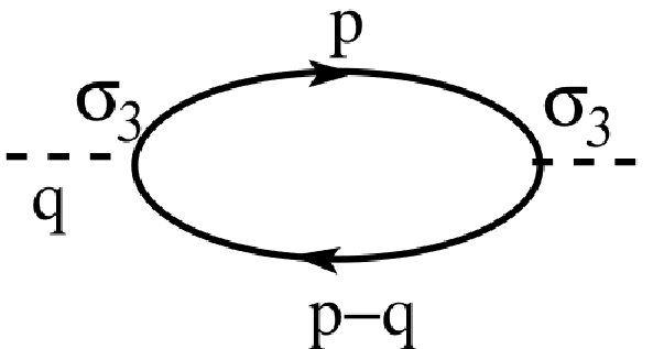
Formally can be considered as a mass term, while are components of a gauge field that emerged due to the deformations of the honeycomb lattice. One recognizes that lowest order in the phonon field contributes only into the mass term, while the emerging -gauge field appears in quadratic over order. Therefore, to leading order of the fermionic fluctuations create an effective action based on the correlator between the ’axial currents’ . Adopting the dimensional regularization scheme one obtains to one loop order, cf. Fig. 3 [Redlich1984; Son2007; apresyan-2017]
| (17) |
written in momentum space. In deriving this expression one has to keep in mind that does not commute with the fermionic propagator, cf. supplement materials.
In the next order in ’s, i.e. to the order , there appear anomalous current-current correlators corresponding to the remaining two space-like components of the gauge field . According to the seminal works of Redlich [redlich84; Redlich1984], Semenoff [Semenoff-1984] and Jakiw [Jackiw], the
| (18) |
where refers to an infinitesimally small bare mass parameter , which was introduced to regularize the infrared divergence and sent to zero after the integration. Variation of the action Eq. (18) creates an anomalous current
| (19) |
The sign () ambiguity of the mass reflects the fact that the mass parameter must not necessarily be positive. As it is always the case with anomalies in perturbative approaches, the anomalous current Eq. (19) appears because the regulator violates the chiral symmetry of the model Eq. (11) explicitly. Due to the finite band width of our lattice model, there is no need for an ultraviolet regularization.
In this case the chiral symmetry is preserved and the anomalous currents cancel each other due to fermion species doubling susskind77. However, if the dynamics of phonons is included into the model, the breaking of the chiral symmetry can occur spontaneously, provided the phonon-phonon interaction strength exceeds a certain critical value. This mechanism was recently investigated by two of us in Refs. [Phonon2016; Phonon2019; Phonon2020].
Conclusions: In the present paper we construct a low energy theory of fermions interacting with deformations of the honeycomb lattice. In contrast to similar studies reported recently in Refs. [Vozmediano2010; Vozmediano-2-2010; Vozmediano2012; Vozmediano2016; Volovik2014; Volovik-2015], where fermions are bound to the flat but distorted sheets, we investigate the case when the effective gauge fields are induced by embedding of a two-dimensional surface into a three-dimensional Euclidean space [Sedrakyan1985; Sedrakyan1987]. In addition to the gauge fields and interaction with 2d gravity of former approaches, our effective theory reveals a non-abelian gauge field. We reduce the 2d gravity (metric) field to deformations of the 3d lattice, which is forming three dimensional phononic fields. The calculation of a anomaly links the current of fermions with phononic field strength which, in principle, can be detected experimentally. It remains for the future to extend the formalism presented here to the curved spaces. The ultimate goal may be to establish an effective low-energy field theory of phonons in the spirit of effective Liouville actions [Polyakov1981; Polyakov1983] accompanied by induced topological (Chern-Simons or Hopf) terms. To some extend though, a number of intermediate ideas in terms of mathematical modeling and its effect on transport were successfully realized in [RandLatt2011].
Acknowledgments. A. Sedrakyan expresses his gratitude to the University Augsburg for hospitality during his stay as visiting professor, where this work was initiated. His work was further supported through the ARC grants 18RF-039 and 18T-1C153. A. Sinner and K. Ziegler were supported by the grants of the Julian Schwinger Foundation for Physics Research.
References
- (1) Y. Hasegawa, R. Konno, H. Nakano, and M. Kohmoto, Zero modes of tight-binding electrons on the honeycomb lattice, Phys. Rev. B 74, 033413 (2006).
- (2) G. Montambaux, F. Piéchon, J.-N. Fuchs, and M.O. Goerbig, Merging of Dirac points in a two-dimensional crystal, Phys. Rev. B 80, 153412 (2009).
- (3) V.M. Pereira, A.H. Castro Neto, and N.M.R. Peres, Tight-binding approach to uniaxial strain in graphene, Phys. Rev. B 80, 045401 (2009).
- (4) G. Montambaux, F. Piéchon, J.-N. Fuchs, and M.O. Goerbig, A universal Hamiltonian for motion and merging of Dirac points in a two-dimensional crystal, Eur. Phys. J. B 72, 509 (2009).
- (5) K. Ziegler and A. Sinner, Lattice symmetries, spectral topology and opto-electronic properties of graphene-like materials, Europhys. Lett. 119, 27001 (2017).
- (6) P. Nualpijit, A. Sinner, and K. Ziegler, Tunable transmittance in anisotropic two-dimensional materials, Phys. Rev. B 97, 235411 (2018).
- (7) A.M. Polyakov, Quantum geometry of bosonic strings, Phys. Lett. B 103, 207 (1981).
- (8) L. Alvarez-Gaumé and E. Witten, Gravitational anomalies, Nucl. Phys. B 234, 268 (1983).
- (9) T. Can, M. Laskin, and P. Wiegmann, Fractional quantum Hall effect in a curved space: Gravitational anomaly and electromagnetic response, Phys. Rev. Lett. 113, 227205 (2014).
- (10) M.A.H. Vozmediano, M.I. Katsnelson, and F. Guinea, Gauge fields in graphene, Phys. Rep. 496, 109 (2010).
- (11) F. de Juan, M. Sturla, and M.A.H. Vozmediano, Space Dependent Fermi Velocity in Strained Graphene, Phys. Rev. Lett. 108, 227205 (2012).
- (12) B. Amorim, A. Cortijo, F. de Juan, A.G. Grushin, F. Guinea, A. Gutiérrez-Rubio, H. Ochoa, V. Parente, R. Roldán, P. San-José, J. Schiefele, M. Sturla, and M.A.H. Vozmediano, Novel effects of strains in graphene and other two dimensional materials, Phys. Rep. 617, 1-54 (2016).
- (13) M. Pretko and L. Radzihovsky, Fracton-Elasticity Duality, Phys. Rev. Lett. 120, 195301 (2018).
- (14) B.A. Dubrovin, A.T. Fomenko, and S.P. Novikov, Modern geometry - methods and applications, Springer, New York (1984).
- (15) A.R Kavalov, I.K. Kostov, and A.G. Sedrakyan, Dynamics of Dirac and Weyl fermions on a two-dimensional surface, Phys. Lett. B 175, 331 (1985).
- (16) A. Sedrakyan and R. Stora, Dirac and Weyl fermions coupled to two-dimensional surfaces: Determinants, Phys. Lett. B 188, 442 (1987).
- (17) F. de Juan, A. Cortijo, and M.A.H. Vozmediano, Dislocations and torsion in graphene and related systems, Nucl. Phys. B 828, 625 (2010).
- (18) G.E. Volovik and M.A. Zubkov, Emergent Horava gravity in graphene, Ann. Phys. 340, 352 (2014).
- (19) G.E. Volovik and M.A. Zubkov, Emergent geometry experienced by fermions in graphene in the presence of dislocations, Ann. Phys. 356, 255 (2015).
- (20) S.W. Jung, S.H. Ryu, W.J. Shin, Y. Sohn, M. Huh, R.J. Koch, C. Jozwiak, E. Rotenberg, A. Bostwick and K.S. Kim, Black phosphorus as a bipolar pseudospin semiconductor, Nat. Mater. 19, 227 (2020).
- (21) D. Wulferding, P. Lemmens, F. Büscher, D. Schmeltzer, C. Felser, and C. Shekhar, Effect of topology on quasi-particle interactions in the Weyl semimetal WP2, arXiv:2004.00328.
- (22) A. Sinner, A. Sedrakyan, and K. Ziegler, Optical conductivity of graphene in the presence of random lattice deformations, Phys. Rev. B 83, 155115 (2011).
- (23) A. Sinner and K. Ziegler, Emergent Chern-Simons excitations due to electron-phonon interaction, Phys. Rev. B 93, 125112 (2016).
- (24) A. Sinner and K. Ziegler, Spontaneous mass generation due to phonons in a two-dimensional Dirac fermion system, Ann. Phys. 400, 262 (2019).
- (25) A.N. Redlich, Parity violation and gauge noninvariance of the effective gauge field action in three dimensions, Phys. Rev. D 29, 2366 (1984).
- (26) T.D. Son, Quantum critical point in graphene approached in the limit of infinitely strong Coulomb interaction, Phys. Rev. B 75, 235423 (2007).
- (27) E. Apresyan, Sh. Khachatryan, and A. Sedrakyan, Current-current correlation function in 3D massive Dirac theory with chemical potential, Mod. Phys. Lett. A 30, 1550035 (2015).
- (28) A.N. Redlich, Gauge noninvariance and parity nonconservation of three-dimensional fermions, Phys. Rev. Lett. 52, 18 (1984).
- (29) G. Semenoff, Condensed-matter simulation of a three-dimensional anomaly, Phys. Rev. Lett. 53, 2449 (1984).
- (30) R. Jackiw, Fractional charge and zero modes for planar systems in a magnetic field, Phys. Rev. D 29, 2375 (1984).
- (31) D.M. Basko and I.L. Aleiner, Interplay of Coulomb and electron-phonon interactions in graphene, Phys. Rev. 77, 041409(R) (2008).
- (32) L. Susskind, Lattice fermions, Phys. Rev. D 16, 3031 (1977).
- (33) A. Sinner and K. Ziegler, Quantum Hall effect induced by electron-phonon interaction, Ann. Phys. 418, 168199 (2020).
- (34) F.D.M. Haldane, Model for a quantum Hall Effect without Landau levels: Condensed-matter realization of the ”parity anomaly”, Phys. Rev. Lett. 61, 2015 (1988).
- (35) A. Polyakov and P.B. Wiegmann, Theory of nonabelian Goldstone bosons in two dimensions, Phys. Lett. B 131, 121 (1983).
Supplemental Materials: Deformation of graphene sheet: Interaction of fermions with phonons
Derivation of Eq. (16)
Writing the diagram depicted in Fig.3 as an algebraic expression yields:
| (S1) | |||||
where . With the Feynman trick
| (S2) |
follows
| (S3) |
where the sign change in the first term is because anticommutes with . Shifting , performing the trace and keeping only rotationally invariant terms yields
| (S4) |
Using formulas of dimensional regularization
| (S5) | |||||
yields
| (S6) |
where the integration over is carried out with the substitution , giving
| (S7) |