Statistical description of dust polarized emission from the diffuse interstellar medium

In the diffuse interstellar medium and at the frequencies of a few hundred GHz, we observe the thermal emission of large grains of dust (Draine 2011, typically grains of radii greater than 50 nm, see e.g.,). These large grains are in thermal equilibrium, absorbing the light of surrounding stars and emitting a black body radiation at typical temperatures of a few tens of K. This emission is polarized due to the statistical alignment between the orientation of aspherical dust grains and the local magnetic field (Andersson et al. 2015), leading to preferential directions of absorption and emission of light, and thus to a polarization of the signal (Planck Collaboration Int. XIX 2015).

Taking these processes into account, a physical model of radiative transfer has been built (Planck Collaboration Int. XX 2015, see derivation and references in). This model provides analytical expressions at a given submillimeter frequency $\nu$ for the Stokes parameters $I,Q,$ and $U$:

where $S_{\nu}$ is the source function which is assumed here to be that of a black body so that $S_{\nu}=B_{\nu}(T_{d})$ with $T_{d}$ the dust temperature, $\tau_{\nu}$ is the optical depth, $p_{0}$ is an intrinsic polarization fraction parameter, $\gamma$ is the angle that the local magnetic field makes with the plane of the sky, and $\phi$ is the angle that the projection of the local magnetic field on the plane of the sky makes with the $x$ direction when $z$ is the line of sight in the HEALPix²² 2 https://healpix.jpl.nasa.gov. (Górski et al. 2005) convention (see Fig. 1).

In the following, we assume uniform values for the intrinsic polarization $p_{0}$ and the dust temperature $T_{d}$, an optically thin medium, and an infinitesimal optical depth equal to ${\mathrm{d}\tau_{\nu}=\sigma_{\nu}n_{\mathrm{H}}\mathrm{d}z}$ where $\sigma_{\nu}$ is the dust opacity (assumed uniform) and $n_{\mathrm{H}}$ is the total gas density. In this case, Eqs. (1)-(3) become:

From these formulæ, Stokes parameters $I$, $Q$, and $U$ appear to be proportional to an integration along the line of sight of quantities depending on the same three variables: the total gas density $n_{\mathrm{H}}$, and the angles $\gamma$ and $\phi$. Therefore we expect a priori some statistical dependencies between $I$, $Q$, and $U$ maps, and a statistical description of these Stokes maps should take into account these dependencies.

These expressions also underline how closely related Stokes $Q$ and $U$ are. Indeed they are defined with respect to a given reference direction (Landi Degl’innocenti & Landolfi 2004, see for example), and any rotation of this reference direction by a given angle $\varphi$ transforms $Q$ and $U$ into rotated quantities $Q^{\prime}$ and $U^{\prime}$ as follows³³ 3 These relations hold for an angle $\varphi$ that is counted positively clockwise from the $x$ direction when the $z$-axis is the line of sight in the HEALPix convention. See Fig. 1.:

These relations can be written in a more compact form introducing complex quantities:

As a consequence, the global phase of $Q+iU$ complex maps is directly related to the reference frame in which we define the angular variables measuring the orientation of the local magnetic field within the plane of the sky. Because of the previous transformation properties, the complex variable $Q+iU$ is more apt to represent linear polarization than $Q$ and $U$ separately (Haverkorn et al. 2004, see e.g.,). Moreover it will be useful to define a statistical description of polarization maps that is independent from this choice of reference frame as we discuss in Sect. 2.3.

Finally, let us discuss the non-Gaussianity of Stokes maps $I$, $Q$, and $U$. We know that the gas and the magnetic field in the diffuse interstellar medium are highly turbulent (Hennebelle & Falgarone 2012), and the nonlinearity involved in the MHD equations that describe their dynamics couples scales. Therefore we expect the statistical properties of the sky maps of $I$, $Q$, and $U$ to be highly non-Gaussian. Unless one can find a mapping of the data that leads to Gaussian statistics, a mere statistical description in terms of power spectra measurements cannot be sufficient to statistically characterize these maps.

Stokes maps $I$ and $Q+iU$ are raw observables of the polarized emission of dust that we first want to transform. Our goal is twofold: to simplify the statistical properties of these observables and to ease the physical interpretation of their properties. In this work, we consider three dimensionless variables based on Stokes maps $I$ and $Q+iU$ to build and interpret a statistical description of polarized light: normalized Stokes variable $\tilde{Q}+i\tilde{U}$, polarization fraction $p$ and complex polarization angle $\exp(2i\psi)$.

We first define the normalized Stokes complex variable ${\tilde{Q}+i\tilde{U}}$ as follows:

with $P=|Q+iU|$ the polarized intensity. Such a definition roughly disentangles the structure of the magnetic field and the structure of dust density at the lowest order. Indeed, assuming a constant orientation of the magnetic field along the line of sight, one gets using Eqs. (4), (5), and (6):

which is independent of the density field $n_{\mathrm{H}}$.

The polarization fraction $p$ and the polarization angle $\psi$ follow the usual definitions:

and

where $\mathrm{atan2}(b,a)$ is the function that returns the angle restricted to $(-\pi,\pi]$ between the positive $x$-axis and the ray to the point $(a,b)$ in the Euclidean plane. Because of the nonlinearity of the $\mathrm{atan2}$ function, we expect the statistics of $\psi$ maps to be unnecessarily complicated compared to those of the original Stokes maps. We thus choose to analyze maps of the complex variable $\exp(2i\psi)$. This variable also avoids dealing with discontinuities of $\psi$ maps that appear where the polarization angle approaches $\pm\pi/2$. Moreover, the statistical properties of $\exp(2i\psi)$ are easier to compare to those of $\tilde{Q}+i\tilde{U}$ since $\tilde{Q}+i\tilde{U}\approx p\exp(2i\psi)$ when $P\ll I$ (which is typically the case).

The WST is a tool from data science that computes statistical descriptions of images that can efficiently discriminate between images which have identical power spectra but distinct higher order moments (Bruna & Mallat 2013). An advantage of this description compared to the direct estimation of higher order moments is that the estimators of the WST coefficients have a low variance and thus do not need a large amount of samples for an accurate estimation. This is because the WST relies on nonexpansive operators (Bruna & Mallat 2013, see). Originally designed to understand the properties of deep convolutional neural networks which have proved successful for classification problems (LeCun et al. 2010; Krizhevsky et al. 2012), this tool also provides a convenient statistical description of astronomical observations of the interstellar medium for total intensity maps (Allys et al. 2019). In this subsection we use the WST to describe the statistical properties of the polarization related maps discussed in the previous section: complex maps $\tilde{Q}+i\tilde{U}$ and $\exp(2i\psi)$, and real map $p$.

Let us briefly recall the definition of the WST of a given 2D real field $I(\textbf{x})$ that is statistically homogeneous⁴⁴ 4 In this work, we restrict our analysis to statistically homogeneous data for simplicity, but this is not a limitation of the methodology as the WST can also be computed locally (Allys et al. 2019, see e.g.,).. For a more complete presentation we refer to Allys et al. 2019 and Bruna & Mallat 2013. The WST relies on convolutions of the target field $I(\textbf{x})$ with a set of $J\times\Theta$ Morlet wavelets $\psi_{j,\theta}$ with ${0\leq j\leq J-1}$ and $\theta\in\{k\pi/\Theta,0\leq k\leq\Theta-1\}$, with $J$ and $\Theta$ two integers. These wavelets $\psi_{j,\theta}$ are the result of the dilation by a factor $2^{j}$ and the rotation by an angle $\theta$ of a mother Morlet wavelet $\Psi$:

A Morlet wavelet is essentially a plane wave modulated by a Gaussian envelope. It is a quite general kind of wavelet to study physical fields and it provides a good angular selectivity (Farge 1992). We recall the definition of the mother Morlet wavelet $\Psi$:

with $\alpha$ and $\beta$ two constants that are adjusted to ensure a zero mean and a unit $L^{1}$ norm, $\textbf{k}_{0}=k_{0}\textbf{e}_{x}$ the wave vector of the plane wave factor, and $\sigma$ the standard deviation of the Gaussian envelope⁵⁵ 5 In practice we choose $k_{0}=3\pi/4\,\mathrm{pixel}^{-1}$ and $\sigma=0.8\,\mathrm{pixel}$ as in Bruna & Mallat 2013.^,66 6 Actually, the Gaussian envelope has an elliptical shape that is not included in Eq. (15) for simplicity. This elliptical shape enhances the angular selectivity of the wavelets.. Convolving a field $I(\textbf{x})$ with a wavelet $\psi_{j,\theta}$ corresponds to a local band-pass filtering of the field at frequencies centered on a mode $\textbf{k}_{j,\theta}=k_{0}2^{-j}\left(\cos\left(\theta\right)\hat{\textbf{e}}_{x}+\sin\left(\theta\right)\hat{\textbf{e}}_{y}\right)$. $J$ and $\Theta$ constants thus correspond respectively to the number of scales and angles that discretize the 2D Fourier space. For a statistically homogeneous real field $I(\textbf{x})$, normalized WST coefficients are defined as follows:

where the averaging operator $\langle\cdot\rangle$ here is simply an average over a map, meaning $\langle I\rangle=\frac{1}{A}\int I(\textbf{x})\mathrm{d}^{2}\textbf{x}$ with $A$ the area of integration, and where the $\star$ symbol stands for the convolution operator. The number of WST coefficients depends on the $J$ and $\Theta$ parameters: we have a single $\bar{S}_{0}$ coefficient, $J\times\Theta$ $\bar{S}_{1}$ coefficients, and $\Theta^{2}\times J\times(J-1)/2$ $\bar{S}_{2}$ coefficients.

These coefficients can be interpreted in the following manner: $\bar{S}_{0}$ is simply the mean of the field, $\bar{S}_{1}(j_{1},\theta_{1})$ is a measure of the amplitude of oscillation of the normalized $I/\langle I\rangle$ field for modes centered on $\textbf{k}_{j_{1},\theta_{1}}$, and finally $\bar{S}_{2}(j_{1},\theta_{1},j_{2},\theta_{2})$ characterizes how the normalized amplitude of oscillation of the field for a mode $\textbf{k}_{j_{1},\theta_{1}}$ is modulated by a mode of oscillation $\textbf{k}_{j_{2},\theta_{2}}$. Accordingly, the $\bar{S}_{1}(j_{1},\theta_{1})$ coefficient characterizes the amplitude at a single oriented scale $(j_{1},\theta_{1})$, while the $\bar{S}_{2}(j_{1},\theta_{1},j_{2},\theta_{2})$ coefficient measures the coupling between two oriented scales $(j_{1},\theta_{1})$ and $(j_{2},\theta_{2})$.

We note that even if the $\bar{S}_{1}$ coefficients characterize the Fourier amplitude of the field under study in the spectral band of the wavelets, they differ in practice from the power spectrum. While the power spectrum can be computed from $L^{2}$ norms of the wavelet transform, the $\bar{S}_{1}$ coefficients are computed with $L^{1}$ norms. One can however recover the power spectrum at a given scale from a quadratic sum of $\bar{S}_{1}$ and $\bar{S}_{2}$ coefficients⁷⁷ 7 See Eq. (9) in Allys et al. 2019.. Notably, we expect a non-Gaussian field to have higher $\bar{S}_{2}$ coefficients compared to those of a Gaussian field with identical power spectrum, and this should be counterbalanced by smaller $\bar{S}_{1}$ coefficients. This is related to the sparsity of the wavelet representation of the data (see Allys et al. 2019 and Bruna & Mallat 2013 for further discussions).

We can extend the previous definition of normalized WST coefficients to statistically homogeneous complex fields such as $\tilde{Q}+i\tilde{U}$ or $\exp(2i\psi)$ as follows:

where we still have $0\leq j_{1},j_{2}\leq J-1$ with $j_{2}>j_{1}$ for $\bar{S}_{2}$ coefficients, but here the main difference is that $0\leq\theta_{1}<2\pi$ and $0\leq\theta_{2}<\pi$. This new range of angles for $\theta_{1}$ is directly related to the complex nature of the $\tilde{Q}+i\tilde{U}$ variable. For a real signal $I(\textbf{x})$, one can easily show that $|I\star\psi_{j_{1},\theta_{1}+\pi}|=|I\star\psi_{j_{1},\theta_{1}}|$, which explains the range of $\theta_{1}$ in Eq. (17). For a complex signal the previous relation does not hold anymore, and we have to consider rotations of the mother wavelet $\Psi$ for angles between $0$ and $2\pi$ (see Mallat 2012, for more details). We note that the range of angles for $\theta_{2}$ is unchanged because $|(\tilde{Q}+i\tilde{U})\star\psi_{j_{1},\theta_{1}}|$ is a real signal. Thus, for a complex field, we end up with twice as many $\bar{S}_{1}$ and $\bar{S}_{2}$ coefficients as for the WST of a real field.

Let us note that this definition of the WST on complex polarization maps $\tilde{Q}+i\tilde{U}$ does not depend on the global phase of $\tilde{Q}+i\tilde{U}$ maps, meaning that the WST coefficients associated to $\tilde{Q}+i\tilde{U}$ maps do not depend on the reference frame mentioned in Sect. 2.1.

In the following, the statistical properties of $p$ maps will be described with the WST coefficients defined in Eqs. (16), (17), and (18), while the statistical properties of $\tilde{Q}+i\tilde{U}$ and $\exp(2i\psi)$ maps will be described with the WST coefficients defined in Eqs. (19), (20), and (21).

Throughout this paper we work with Stokes maps which are directly computed as integrations along a given direction of 3D simulated cubes of data extracted from a numerical simulation of magnetized interstellar turbulence (this given direction of integration corresponds to the line of sight for observations). As a first step, working with MHD simulations instead of observational data is a stepping-stone to relate our statistical descriptions to physics where we avoid the difficulty of dealing with data noise.

We use a MHD simulation designed to study the biphasic nature of the diffuse interstellar medium (Bellomi et al., in prep.). The simulation uses the adaptive mesh refinement code RAMSES (Teyssier 2002; Fromang et al. 2006) to solve the equations of ideal MHD as described in Iffrig & Hennebelle 2017, neglecting self-gravity and taking into account heating and cooling processes of the gas. Turbulent forcing is applied to inject kinetic energy and balance numerical dissipation so that the simulation reaches a statistical steady state. In practice this turbulent forcing consists in a large-scale stochastic force field (a three component Ornstein-Uhlenbeck process defined in spectral space). Details on the turbulent forcing model can be found in Schmidt et al. 2006.

The simulation volume is a $(50\penalty\ \mathrm{pc})^{3}$ box divided into $512^{3}$ cells with periodic boundary conditions. At $t=0$ the gas has uniform properties with a density $n_{\mathrm{H}}=1.5\penalty\ \mathrm{cm}^{-3}$ and a temperature $T=8000\penalty\ \mathrm{K}$, and the magnetic field is also uniform, with $\textbf{B}_{0}=B_{0}\textbf{e}_{x}$ and $B_{0}\sim 3.8\penalty\ \mathrm{\mu G}$. In steady state, the turbulent forcing leads to an approximate velocity dispersion $\sigma_{v}\sim 2.6\penalty\ \mathrm{km/s}$. This gives a turnover time at large scale $\tau_{L}\approx 18.8\penalty\ \mathrm{Myr}$. Finally, an isotropic Habing radiation field is applied at the boundaries of the box. Its intensity is scaled by a factor $G_{0}=1$ (Draine 2011, for a definition, see).

Once the simulation has reached a statistical steady state, we extract 14 snapshots that are approximately statistically independent using an approach similar to Federrath et al. 2009. In practice we make sure that two consecutive snapshots correspond to a minimal time evolution of $\delta\tau=1.25\penalty\ \mathrm{Myr}$ which is roughly ten percent of $\tau_{L}$. The phenomenology of turbulence in the sense of Kolmogorov shows that the turnover time $\tau_{l}$ at a given scale $l$ scales as $l^{2/3}$ (Frisch 1995). This scaling holds for incompressible hydrodynamical turbulence only but we assume for the sake of simplicity that it extends reasonably well to ideal compressible MHD. At the range of scales considered in the following, we find that $\delta\tau$ is about fives times smaller than the corresponding largest value of $\tau_{l}$. Although this value is not completely satisfactory, we assume that the snapshots are statistically independent.

We can compute a set of Stokes maps $I$, $Q$, and $U$ for each of these snapshots using Eqs. (4), (5), and (6) and choosing the $z$-axis of the cubes as the direction of integration. We note that this integration procedure is identical to the one used in Planck Collaboration Int. XX 2015. We choose a typical value for the polarization fraction parameter $p_{0}=0.2$ and arbitrary values for $\sigma_{\nu}$ and $T_{d}$ as these only determine the global amplitude of $I$, $Q$ and $U$ maps but do not impact the analysis. These maps are relevant for any frequency $\nu$ provided that the dust emission remains optically thin. Then from these Stokes maps we compute the associated maps $P$, $\tilde{Q}$, $\tilde{U}$, $p$, $\cos(2\psi)$, and $\sin(2\psi)$ which are the transformations of the Stokes observables defined in Sect. 2.2. Finally, we end up with a set of 14 maps for each of these variables.

We point out that the initial conditions of the MHD simulations are anisotropic because of the initial direction of the uniform magnetic field. This anisotropy remains once the simulation has reached steady state, due to magnetic flux conservation, and the value of the mean magnetic field is $\bar{\textbf{B}}\approx\textbf{B}_{0}$. Because the direction of integration chosen to compute the previous Stokes maps is orthogonal to the direction of the mean magnetic field $\bar{\textbf{B}}$ in the simulation, we refer to the previous sets of maps using the $\bot$ symbol. For instance, the $p_{\bot}$ data set refers to the set of 14 maps of polarization fraction $p$ computed from the 14 maps $I$, $Q$, and $U$ for which the $z$-axis was the axis of integration. We similarly compute Stokes maps integrating along the $x$-axis which is the direction of the mean magnetic field. This results in a set of maps that are statistically isotropic and from which we also compute the associated maps $P$, $\tilde{Q}$, $\tilde{U}$, $p$, $\cos(2\psi)$, and $\sin(2\psi)$. We use the $\parallel$ symbol to refer to these sets of maps.

We use for this work eight data sets, each one comprising 14 statistically independent maps. The various maps presented in the last subsection define 6 data sets: $\exp(2i\psi)_{\bot},p_{\bot},\tilde{Q}_{\bot}+i\tilde{U}_{\bot}$, $\exp{(2i\psi)}_{\parallel},p_{\parallel}$, and $\tilde{Q}_{\parallel}+i\tilde{U}_{\parallel}$. In addition, we also analyze phase randomized data sets $R[\tilde{Q}_{\bot}+i\tilde{U}_{\bot}]$ and $R[\tilde{Q}_{\parallel}+i\tilde{U}_{\parallel}]$ built respectively from the $\tilde{Q}_{\bot}+i\tilde{U}_{\bot}$ and $\tilde{Q}_{\parallel}+i\tilde{U}_{\parallel}$ data sets.

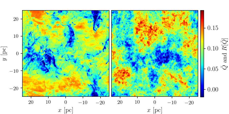
We define $R[\cdot]$ to be the operator that acts on a map by randomizing the phases of the map in Fourier space, meaning that the new phases are drawn from a uniform distribution on $[0,2\pi)$. We note that the modulus of the Fourier coefficients are retained so that the power spectrum is also unchanged. The phase information of an image is tightly bound to its structure (Oppenheim & Lim 1981) and the main effect of the $R[\cdot]$ operator is to severely damage the structure of the image. We use phase randomization as an approximation to Gaussianization⁸⁸ 8 Stationary Gaussian random fields (GRFs) do have uniformly distributed phases on $[0,2\pi)$ but this property alone does not define them (Wandelt 2013, see).. We could have used a standard Gaussian random field generation (Kroese & Botev 2015, see e.g.,), however we found out that the two approaches give similar results. In practice $R[\tilde{Q}_{\bot}+i\tilde{U}_{\bot}]$ (respectively $R[\tilde{Q}_{\parallel}+i\tilde{U}_{\parallel}]$) refers to the set of 14 maps produced by randomizing separately $\tilde{Q}$ and $\tilde{U}$ maps from the $\tilde{Q}_{\bot}+i\tilde{U}_{\bot}$ data set (respectively $\tilde{Q}_{\parallel}+i\tilde{U}_{\parallel}$). Technical details about phase randomization can be found in Appendix B, as well as an example of a phase randomized map for $R[\tilde{Q}_{\bot}+i\tilde{U}_{\bot}]$ in Fig. 16.

Figure 2 shows examples of maps for $I_{\bot}$, $Q_{\bot}$, $U_{\bot}$, $P_{\bot}$, $\tilde{Q}_{\bot}$, $\tilde{U}_{\bot}$, $p_{\bot}$, $\cos(2\psi)_{\bot}$, and $\sin(2\psi)_{\bot}$ data sets, while Fig. 3 shows examples of maps for the corresponding $\parallel$ data sets. These figures show maps that all rely on the same snapshot of a MHD simulation. We draw the attention of the reader to a few points. First, we clearly see filamentary patterns on these maps that will demand a statistical description involving higher orders statistics compared to simple power spectra. We also note that $P$ is an order of magnitude lower than the intensity $I$ (this is due to the value of the polarization fraction parameter $p_{0}$), hence we have approximately $\tilde{Q}+i\tilde{U}\approx(Q+iU)/I$ so that $p$ roughly behaves as the modulus of $\tilde{Q}+i\tilde{U}$, and $2\psi$ roughly behaves as its complex argument. Next, we note that the magnitude of $p_{\parallel}$ is unsurprisingly much lower than that of $p_{\bot}$ as the direction of the projection of the local magnetic field on the plane of the sky is much less coherent along the line of sight when the line of sight corresponds to the direction of the mean magnetic field. Finally, we see on the $\cos(2\psi)_{\bot}$ map that the anisotropy of the magnetic field in the simulation leads to values that are concentrated close to 1.

We now focus on the WST coefficients associated with the ${\tilde{Q}_{\bot}+i\tilde{U}_{\bot}}$ data set, but the following reasoning remains valid for the other data sets, including those related to $\exp(2i\psi)$ and $p$.

For the 14 maps of the $\tilde{Q}_{\bot}+i\tilde{U}_{\bot}$ data set, we compute the WST coefficients for $J=7$ and $\Theta=8$ (see Eqs. (19), (20), and (21)). $J$ could have been fixed to a higher value for $512\times 512$ maps, but because of our limited number of maps we chose to restrict our statistical description to scales for which we have a sufficient number of modes for reliable estimations. We give in Table 1 the correspondence between the scale index $j$ and the central wavelength of the related dilated Morlet wavelet both in pixel units and in dimensional units (related to the MHD simulation).

These $J$ and $\Theta$ values lead for each map to 112 $\bar{S}_{1}$ coefficients and 2688 $\bar{S}_{2}$ coefficients. Adding to this the $\bar{S}_{0}$ coefficient, we end up with 2801 coefficients per map. We define mean $\bar{S}_{0}$, $\bar{S}_{1}$ and $\bar{S}_{2}$ coefficients as means of the WST coefficients over the 14 maps and we also compute the standard deviation of the mean for each of these coefficients assuming that the maps are statistically independent.

Figures 4 and 5 represent (in blue) respectively $\bar{S}_{1}(j_{1},\theta_{1})$ coefficients and a representative subsample of $\bar{S}_{2}(j_{1},\theta_{1},j_{2},\theta_{2})$ coefficients (for $j_{1}=1$) on a logarithmic scale, for $\tilde{Q}_{\bot}+i\tilde{U}_{\bot}$. In both figures, we represent the multivariate functions $\bar{S}_{1}$ and $\bar{S}_{2}$ in a lexicographical order for the $(j_{1},\theta_{1})$ and $(j_{1},\theta_{1},j_{2},\theta_{2})$ variables, respectively. Vertical gray lines help to mark increments of these variables.

In Fig. 4, we see that for a fixed scale $j_{1}$ a smooth pattern emerges with respect to the angular variable $\theta_{1}$. Because of the definition of $\bar{S}_{1}$ coefficients, at fixed $j_{1}$, $\log_{2}(\bar{S}_{1})(j_{1},\cdot)$ functions must be $2\pi$-periodic, but here the smooth pattern appears to be $\pi$-periodic. While it is not surprising to get smooth angular patterns that reflect the regularity of physical processes, this $\pi$-periodicity with respect to the angular variable $\theta_{1}$ was unexpected.

We can nevertheless explain it by noticing that:

because for Morlet wavelets we have $\psi_{j,\theta}^{*}=\psi_{j,\theta+\pi}$⁹⁹ 9 The ^∗ symbol stands for the complex conjugate.. Hence, saying that $\log_{2}(\bar{S}_{1})(j_{1},\cdot)$ functions are $\pi$-periodic amounts to saying that $\tilde{Q}+i\tilde{U}$ and $\tilde{Q}-i\tilde{U}$ have the same WST first order statistics.

We can identify the same kind of regularity properties for $\bar{S}_{2}$ coefficients in Fig. 5. Since $\bar{S}_{2}$ coefficients depend on four variables, two of which are angular variables $\theta_{1}$ and $\theta_{2}$, it is more complicated to see this angular regularity, but Fig. 6 helps us to exhibit this regularity by plotting $\bar{S}_{2}$ coefficients as a function of angular variables $\theta_{1}$ and $\theta_{2}$ when $j_{1}=1$ and $j_{2}=3$. Smooth angular patterns appear on this surface which is parameterized by $\theta_{1}$ and $\theta_{2}$. In particular we see that $\theta_{1}-\theta_{2}=c$ cuts of this surface for arbitrary constants $c$ give roughly constant $\bar{S}_{2}$ coefficients. On this example we thus expect most of the angular modulation to depend on the $\theta_{2}-\theta_{1}$ variable.

The smooth periodic patterns identified in the $\tilde{Q}_{\bot}+i\tilde{U}_{\bot}$ WST coefficients suggest that a simplification of the WST statistical description is possible, through an adequate modeling of its angular dependencies. The purpose of such a modeling of the WST coefficients is twofold: 1) lowering the dimensionality of the statistical description of our data, and 2) providing an interpretable representation of these angular dependencies in terms of considerations of isotropy and anisotropy of the data.

We model the regularity of WST coefficients with respect to angular variables $\theta_{1}$ and $\theta_{2}$ using the RWST model introduced in Allys et al. 2019. It is remarkable that a model developed for total intensity maps may be applied to $\tilde{Q}+i\tilde{U}$ complex Stokes maps of polarized thermal emission of dust, without any modification. This highlights the generality of such an angular modeling of the WST coefficients for maps of dust emission, and this model may surely be extended to other kinds of complex-valued fields in physics. We present in Appendix A the RWST model in terms of Fourier series expansions and rephrase the characteristics of this generality.

We now briefly recall the RWST model, and refer the reader to Allys et al. 2019 for more details.

In the RWST model, the $\bar{S}_{1}$ coefficients are written as:

where $\hat{S}_{1}^{\mathrm{iso}}(j_{1})$, $\hat{S}_{1}^{\mathrm{aniso}}(j_{1})$, and $\theta^{\mathrm{ref},1}(j_{1})$ are the parameters of this angular model for scale $j_{1}$. This model thus depends on $3\times J$ parameters. We also enforce $\hat{S}_{1}^{\mathrm{aniso}}(j_{1})\geq 0$ in order to lift a degeneracy between the $\hat{S}_{1}^{\mathrm{aniso}}(j_{1})$ and $\theta^{\mathrm{ref},1}$ parameters. $\hat{S}_{1}^{\mathrm{iso}}(j_{1})$ quantifies the isotropic component of the data fluctuations at a scale $j_{1}$, while $\hat{S}_{1}^{\mathrm{aniso}}(j_{1})$ defines a measure of the angular modulation of the coefficients at scale $j_{1}$, introducing a reference angle $\theta^{\mathrm{ref},1}(j_{1})$ that defines a privileged direction in the maps ¹⁰¹⁰ 10 We note that Eq. (3.4) defines an angular model of the logarithm of the WST coefficients that turns angular modulations of the WST coefficients into additive corrections $\hat{S}_{1}^{\mathrm{aniso}}(j_{1})\cos\left(2\left[\theta_{1}-\theta^{\mathrm{ref},1}\left(j_{1}\right)\right]\right)$ to the isotropic amplitude of fluctuations $\hat{S}_{1}^{\mathrm{iso}}(j_{1})$. We use a base 2 logarithm to be consistent with the base 2 definition of scales $j_{1}$ and $j_{2}$..

Similarly, the RWST model for $\bar{S}_{2}$ coefficients reads:

where $\hat{S}_{2}^{\mathrm{iso},1}(j_{1},j_{2})$, $\hat{S}_{2}^{\mathrm{iso},2}(j_{1},j_{2})$, $\hat{S}_{2}^{\mathrm{aniso},1}(j_{1},j_{2})$, $\hat{S}_{2}^{\mathrm{aniso},2}(j_{1},j_{2})$, and $\theta^{\mathrm{ref},2}(j_{1},j_{2})$ are the parameters of this angular model for each pair of scales $(j_{1},j_{2})$. As we have $j_{2}>j_{1}$, we end up with $5\times J\times(J-1)/2$ parameters for this model. Here again we make sure that $\hat{S}_{2}^{\mathrm{aniso},1}(j_{1},j_{2})\geq 0$ to avoid any parameter degeneracy. $\hat{S}_{2}^{\mathrm{iso},1}$ measures the overall amplitude of coupling between the scales $j_{1}$ and $j_{2}$. $\hat{S}_{2}^{\mathrm{iso},2}$ represents the amplitude of the modulation due to the relative orientation of the wavelets $\psi_{j_{1},\theta_{1}}$ and $\psi_{j_{2},\theta_{2}}$, and we interpret it as a signature of filamentary structures at a given scale. Indeed for an oriented filamentary structure, we expect the $\bar{S}_{2}$ coefficients to peak when $\theta_{2}=\theta_{1}$ and to reach a minimum when $\theta_{2}=\theta_{1}+\pi/2$. Finally, $\hat{S}_{2}^{\mathrm{aniso},1}$ and $\hat{S}_{2}^{\mathrm{aniso},2}$ are measures of the anisotropic properties of the data in second order WST coefficients, here decoupling $\theta_{1}$ and $\theta_{2}$ contributions.

In practice, for a given data set, this RWST model of the angular dependencies is fitted to the first order WST coefficients for every scale $j_{1}$, and to the second order WST coefficients for every pair of scales $(j_{1},j_{2})$ (with $j_{2}>j_{1}$). The accuracy of these multiple fits is quantified with $\chi_{\mathrm{r}}^{2}$ statistics as described in Allys et al. 2019. Since it is not possible to properly estimate the full covariance matrix with only 14 samples per coefficient, the uncertainties affecting the WST coefficients for a given data set are simply estimated from the sample variance across the various simulation snapshots.

However an important correlation of the first order WST coefficients across angles for each scale $j_{1}$ needs to be taken into account to properly estimate statistical uncertainties. For each sample we compute a mean coefficient across angles for a given scale and subtract this mean before computing the statistical uncertainties¹¹¹¹ 11 This decreases the effective number of degrees of freedom by one when computing $\chi_{\mathrm{r}}^{2}$ values.. This mitigates most of the correlation between WST coefficients at the same scale $j_{1}$.

Figure 7 shows the $\chi_{\mathrm{r}}^{2}$ values for both $\log_{2}(\bar{S}_{1})$ and $\log_{2}(\bar{S}_{2})$ fits for the $\tilde{Q}_{\bot}+i\tilde{U}_{\bot}$ data set. The $\chi^{2}_{\mathrm{r}}$ values are globally close to 1 except at low $j_{1}$ for $\chi_{\mathrm{r}}^{2,\mathrm{S_{1}}}$ and at low $j_{2}-j_{1}$ for $\chi_{\mathrm{r}}^{2,\mathrm{S_{2}}}$. This deterioration of the goodnesses of the fits is due to a pixellization effect at small scales, and may be fixed by adding adequate lattice terms in the RWST model, as described in the appendix C of Allys et al. 2019. This is shown for our data in Appendix C.1. We note that these additional terms do not affect the values of the coefficients corresponding to the original RWST model. Finally, the same RWST model applies to the other data sets used in this work, including $\exp(2i\psi)$ and $p$ data sets, and we get for all of them similar $\chi_{\mathrm{r}}^{2}$ values.

In Figs. 4 and 5 we show the RWST fit overplotted on a selection of first and second order WST coefficients, and also show the corresponding normalized residuals. The curves are globally in good agreement and the flaws of the RWST model due to numerical effects at low $j_{1}$ and $j_{2}-j_{1}$ appear as clear patterns in the residuals. Additional figures in appendix C.1 show how these artifacts may be taken into account.

In the end, the RWST coefficients define statistical descriptions of the data sets in terms of simple considerations of isotropy and anisotropy with respect to a reference direction. Furthermore, these statistical descriptions exhibit much lower dimensionality, with a total of 127 coefficients (including $\bar{S}_{0}$ coefficient in the description) compared to the original 2801 WST coefficients in the case of complex variables $\tilde{Q}+i\tilde{U}$ and $\exp(2i\psi)$¹²¹² 12 For $p$ maps, the WST descriptions consist of 1401 coefficients., thus providing a very large compression of the statistical information contained in the WST coefficients.

Figure 8 presents $\hat{S}_{1}^{\mathrm{iso}}+\log_{2}(\bar{S}_{0})$ coefficients as a function of scale for $\tilde{Q}_{\bot}+i\tilde{U}_{\bot},\tilde{Q}_{\parallel}+i\tilde{U}_{\parallel}$, $R[\tilde{Q}_{\bot}+i\tilde{U}_{\bot}]$ and $R[\tilde{Q}_{\parallel}+i\tilde{U}_{\parallel}]$ data sets. We note that the $\log_{2}(\bar{S}_{0})$ term cancels the normalization of the $\bar{S}_{1}$ WST coefficients defined in Eq. (20) in order to analyze the statistics of $\tilde{Q}+i\tilde{U}$ (and not the statistics of $(\tilde{Q}+i\tilde{U})/\langle|\tilde{Q}+i\tilde{U}|\rangle$). We see that $\hat{S}_{1}^{\mathrm{iso}}+\log_{2}(\bar{S}_{0})$ levels which measure an amplitude of fluctuations of the signal, per scale, are higher for $\tilde{Q}_{\bot}+i\tilde{U}_{\bot}$ and $R[\tilde{Q}_{\bot}+i\tilde{U}_{\bot}]$ than for the corresponding $\parallel$ data sets. This shows that the amplitudes differ depending on the orientation of the mean magnetic field with respect to the line of sight. We have more fluctuations within $\tilde{Q}+i\tilde{U}$ maps when the mean magnetic field is in the plane of the sky.

The differences between the $\tilde{Q}+i\tilde{U}$ data set and its corresponding randomized counterpart $R[\tilde{Q}+i\tilde{U}]$ (in both $\bot$ and $\parallel$ cases) illustrate the difference between $\bar{S}_{1}$ coefficients and the power spectrum. Indeed, $\tilde{Q}+i\tilde{U}$ and $R[\tilde{Q}+i\tilde{U}]$ maps share the same power spectrum but have different $\bar{S}_{1}$ coefficients. The fact that the $R[\cdot]$ operator increases the $\bar{S}_{1}$ values leaving the power spectrum unchanged shows that it reduces the sparsity of these maps (see discussion in Sect. 2.3). This feature underlines the non-Gaussianity of the $\tilde{Q}+i\tilde{U}$ data set and we therefore expect its second order coefficients to be higher compared to those of the corresponding randomized data set. We note that these differences wear off at large scales. We interpret this as statistical evidence that the non-Gaussianity of $\tilde{Q}+i\tilde{U}$ maps decreases at large scales. This result may reflect a characteristic of interstellar turbulence but could also follow from the fact that we start to probe the Gaussian distribution of the turbulent forcing of the simulation.

In Fig. 9, we compare $\tilde{Q}+i\tilde{U}$ $\hat{S}_{1}^{\mathrm{iso}}$ coefficients to those of $p$ and $\exp(2i\psi)$ for respectively $\parallel$ and $\bot$ data sets. Since we have $\tilde{Q}+i\tilde{U}\approx p\exp(2i\psi)$ we would like to compare the relative contributions of $\hat{S}_{1}^{\mathrm{iso}}$ coefficients of $\tilde{Q}+i\tilde{U}$ maps, but this seems more complicated than expected as we found out that a proper comparison through $\hat{S}_{1}^{\mathrm{iso}}$ coefficients highly depends on the choice of normalization of the WST coefficients for $p$.

$\hat{S}_{1}^{\mathrm{iso}}$ coefficients roughly range from $-4.5$ to $-3.0$ for $\exp({2i\psi})_{\parallel}$ while they range from $-5.8$ to $-4.2$ for $\exp({2i\psi})_{\bot}$. These differences indicate larger fluctuations of the polarization angle when the mean magnetic field is along the line of sight compared to when the mean magnetic field is in the plane of the sky. Since the average polarization fraction $p$ is lower when the mean magnetic field is along the line of sight ($\bar{S}_{0}\approx 0.03$ for $p_{\parallel}$ compared to $\bar{S}_{0}\approx 0.1$ for $p_{\bot}$) this feature is consistent with the anti-correlation observed with polarization data between the angle dispersion function $\mathcal{S}$ and the polarization fraction $p$ (Planck Collaboration Int. XX 2015; Planck Collaboration XII 2019; Fissel et al. 2016).

$\hat{S}_{1}^{\mathrm{aniso}}$ coefficients measure the angular modulation of the first order WST coefficients. They are presented in Fig. 10 for all data sets. We see that this anisotropy is much larger for $\bot$ data sets than for $\parallel$ ones. The $p_{\bot}$ data set constitutes an exception among the $\bot$ data sets as it has a rather low anisotropy level. These differences are not surprising as we expect a stronger anisotropy when the mean magnetic field is in the plane of the sky, while statistical isotropy is expected when integrating along the mean magnetic field. For larger scales, we see an increase of these coefficients for $\bot$ data sets. This trend has already been observed on observational data of the Polaris flare in total intensity (Allys et al. 2019) and deserves a closer examination.

As explained in Sect. 3.1 the large scales of consecutive snapshots could be correlated to some extent. To assess the potential impact of these correlations on our analysis, we have computed separate RWST statistics for three maps of the ${\tilde{Q}_{\bot}+i\tilde{U}_{\bot}}$ data set corresponding to snapshots that are sufficiently distant in time to rightfully assume the independence (we choose $6\times\delta\tau$ instead of $\delta\tau$). The increase of $\hat{S}_{1}^{\mathrm{aniso}}$ coefficients remains significant for each map, which demonstrates that this trend is not a consequence of correlations among snapshots.

Reference angles $\theta^{\mathrm{ref},1}$ also presented in Fig. 10 show that the preferential direction identified for anisotropic $\bot$ data sets is the direction corresponding to $\theta^{\mathrm{ref},1}=0$ for all scales $j_{1}$. Such a value of the reference angle indicates a statistical tendency for structures, including filaments, to be elongated vertically rather than horizontally, that is, along the $y$ axis in Fig. 2. This corresponds to an elongation which is orthogonal to the mean magnetic field. This result is to be compared in further works to the abundant literature on the relative orientation between magnetic fields and structures traced by interstellar dust (Hennebelle & Inutsuka 2019, for a review, see).

The reference angle found for $\parallel$ data set is well defined and approximately equal to $\pi/4$ for all scales while the anisotropy levels are close to zero. These values of $\theta^{\mathrm{ref},1}$ are surprising because we were not expecting any anisotropy for these data sets. By examining the RWST statistics separately for each map, for each of the corresponding data sets, we found out that these surprising values correspond to an intermittent rise of the anisotropy level that appears in a few consecutive snapshots of the simulation. In this case where the level and direction of anisotropy are not coherent over snapshots, the mean coefficient gives an incomplete view of the anisotropic properties of the simulation. Notably, even with significant levels of anisotropy per map, if the reference angles are incoherent, we expect the mean level of anisotropy to be small. We found out that this is what happens for the $p_{\bot}$ data set, where $\hat{S}_{1}^{\mathrm{aniso}}$ coefficients are relatively small while $\theta^{\mathrm{ref},1}$ coefficients clearly deviate from zero.

$R[\tilde{Q}+i\tilde{U}]$ maps are Gaussian approximations of $\tilde{Q}+i\tilde{U}$ maps, and we have already exhibited differences between these data sets in their first order RWST coefficients in Sect. 4.1. Similarly, second order RWST coefficients show remarkable differences that highlight the non-Gaussianity of the $\tilde{Q}_{\bot}+i\tilde{U}_{\bot}$ and $\tilde{Q}_{\parallel}+i\tilde{U}_{\parallel}$ data sets. The two dominant second order RWST coefficients $\hat{S}_{2}^{\mathrm{iso},1}$ and $\hat{S}_{2}^{\mathrm{iso},2}$ presented in Fig. 11 display clearly distinct patterns between the original data sets and the randomized ones on the example of the $\bot$ data sets. First, $\hat{S}_{2}^{\mathrm{iso},1}$ and $\hat{S}_{2}^{\mathrm{iso},2}$ coefficients are globally smaller for the $R[\tilde{Q}+i\tilde{U}]$ data sets, which is in line with what we had foreseen in Sect. 4.1. In addition, $\hat{S}_{2}^{\mathrm{iso},1}$ coefficients for $R[\tilde{Q}+i\tilde{U}]$ show a scale invariance property: $\hat{S}_{2}^{\mathrm{iso},1}$ coefficients only depend on the difference $j_{2}-j_{1}$. We point out that these scale invariant patterns are signatures of scale invariant Gaussian processes (Bruna et al. 2015) and have already been observed for fractional Brownian motions processes in Allys et al. 2019.

$\hat{S}_{2}^{\mathrm{iso},2}$ coefficients also show two distinct trends: the coefficients quickly tend to zero when $j_{2}-j_{1}$ increases for $R[\tilde{Q}+i\tilde{U}]$ while coefficients tend to strictly positive values for the largest $j_{2}-j_{1}$ values for non randomized data sets $\tilde{Q}+i\tilde{U}$. This result is related to the filamentary structure of the non randomized maps, because a filamentary structure involves a modulation of the WST coefficients as a function of the angle difference $\theta_{2}-\theta_{1}$. We see the same trend in Fig. 12 for the $\hat{S}_{2}^{\mathrm{iso},2}$ coefficients of the other non randomized data sets which all present filamentary structures. For all data sets, and fixed $j_{1}$ values, $\hat{S}_{2}^{\mathrm{iso},2}$ coefficients decrease as a function of $j_{2}$. This property seems to be general. We also expect a signal due to the imprint of the wavelets in the $\hat{S}_{2}^{\mathrm{iso},2}$ coefficients that would increase their values when $j_{2}$ is close to $j_{1}+1$.

We see in Fig. 11 that the differences between the $\tilde{Q}_{\bot}+i\tilde{U}_{\bot}$ data set and its randomized counterpart decrease for the highest $j_{1}$ values. Here again, this shows that the non-Gaussianity of ${\tilde{Q}+i\tilde{U}}$ maps decreases at large scales. This is consistent with what we have already pointed out in Sect. 4.1 for $\hat{S}_{1}^{\mathrm{iso}}$ coefficients and we interpret this trend similarly.

Second order anisotropic coefficients $\hat{S}_{2}^{\mathrm{aniso},1},\hat{S}_{2}^{\mathrm{aniso},2}$, and $\theta^{\mathrm{ref},2}$ essentially show consistent results with first order anisotropic coefficients both in terms of amplitude and direction of anisotropy. They have generally smaller values compared to those of isotropic coefficients $\hat{S}_{2}^{\mathrm{iso},1}$ and $\hat{S}_{2}^{\mathrm{iso},2}$. We do not show these coefficients here as we do not discuss them any further in this work.

If synthetic total intensity maps generated from a RWST description have already been produced in Allys et al. 2019, in this paper we extend and improve this procedure for complex polarization maps $\tilde{Q}+i\tilde{U}$. We give in this subsection some technical details on the implementation but details on the mathematical formalism can be found in Bruna & Mallat 2019.

The generation of synthetic maps is an iterative process that consists in the minimization of a loss function $\mathcal{L}$ in pixel space. Hence this optimization problem is defined in practice in a space of dimension $512^{2}$. Starting from a realization of a complex Gaussian white noise map $X_{0}=\tilde{Q}_{0}+i\tilde{U}_{0}$, successive maps $\{X_{k}\}$ are built with a quasi-Newton method. We use a L-BFGS-B algorithm, although we do not impose any boundary to the values of the pixels. Technical details on quasi-Newton methods and L-BFGS-B algorithm can be found in Fletcher 1987 and Byrd et al. 1995.

In the following, one specific map $X^{\mathrm{r}}=\tilde{Q}^{\mathrm{r}}+i\tilde{U}^{\mathrm{r}}$ of the data set on which the RWST description is built serves as a reference for comparison with the synthetic maps. Because our WST and RWST analyses does not extend to the largest scales, we have no statistical information on these. Thus, we replace the largest scales of $X_{0}$ with those of $X^{\mathrm{r}}$ to address this gap in a deterministic way¹³¹³ 13 We note that such an approach cannot supply the statistical information concerning the couplings between the largest scales with smaller ones.. Formally, noting $\mathcal{F}[X_{0}]$ the Fourier transform of $X_{0}$ initially drawn as a realization of a Gaussian white noise we set:

where $k_{\mathrm{min}}$ is the wave number corresponding to the largest scale probed by the WST. For $J=7$, using Table 1 we have $k_{\mathrm{min}}\approx 2\pi/171\approx 0.037$ pixel^-1. In practice, 25 Fourier modes out of $512^{2}$ are set by this procedure. Even if in our case this value of $k_{\mathrm{min}}$ is related to an ad hoc modeling decision ($J$ value), we point out that statistical approaches are not always relevant at all scales for the analysis of the diffuse ISM. For example, in a turbulent medium we know that injection scales generally correspond to specific events (e.g., a supernova) for which a statistical description has little meaning, while a statistical description is relevant to describe the inertial range. Moreover, the WST of an image does not adequately characterize its one-point statistics, so in the following we also constrain these for the synthetic maps using $X^{\mathrm{r}}$ one-point statistics as a reference.

We define the loss function $\mathcal{L}$ of a complex image $X=\tilde{Q}+i\tilde{U}$ as follows:

with $\mathcal{L}_{\mathrm{WST}}[X]$ the loss function constraining the WST coefficients of $X$, $\mathcal{L}_{\mathrm{one-point}}[\tilde{Q}]$ (respectively $\mathcal{L}_{\mathrm{one-point}}[\tilde{U}]$) that constraining a few one-point moments of $\tilde{Q}$ (respectively $\tilde{U}$), and $\mu$ a weighting coefficient balancing the importance of one-point moments constraints with that of WST coefficients constraints. More specifically we set:

References

- Abazajian et al. (2019) Abazajian, K., Addison, G., Adshead, P., et al. 2019, arXiv e-prints, arXiv:1907.04473
- Adak et al. (2019) Adak, D., Ghosh, T., Boulanger, F., et al. 2019, arXiv e-prints, arXiv:1906.07445
- Ade et al. (2019) Ade, P., Aguirre, J., Ahmed, Z., et al. 2019, J. Cosmology Astropart. Phys., 2019, 056
- Allys et al. (2019) Allys, E., Levrier, F., Zhang, S., et al. 2019, A&A, 629, A115
- Andersson et al. (2015) Andersson, B. G., Lazarian, A., & Vaillancourt, J. E. 2015, ARA&A, 53, 501
- Aylor et al. (2019) Aylor, K., Haq, M., Knox, L., Hezaveh, Y., & Perreault-Levasseur, L. 2019, arXiv e-prints, arXiv:1909.06467
- BICEP2 Collaboration (2018) BICEP2 Collaboration. 2018, Physical Review Letters, 121, 221301
- BICEP2/Keck Array and Planck Collaborations (2015) BICEP2/Keck Array and Planck Collaborations. 2015, Phys. Rev. Lett., 114, 101301
- Bruna & Mallat (2013) Bruna, J. & Mallat, S. 2013, IEEE Transactions on Pattern Analysis and Machine Intelligence, 35, 1872
- Bruna & Mallat (2019) Bruna, J. & Mallat, S. 2019, Mathematical Statistics and Learning, 1, 257
- Bruna et al. (2015) Bruna, J., Mallat, S., Bacry, E., & Muzy, J.-F. 2015, The Annals of Statistics, 43, 323
- Byrd et al. (1995) Byrd, R., Lu, P., Nocedal, J., & Zhu, C. 1995, SIAM Journal on Scientific Computing, 16, 1190
- Chuss et al. (2019) Chuss, D. T., Andersson, B. G., Bally, J., et al. 2019, ApJ, 872, 187
- Clark & Hensley (2019) Clark, S. E. & Hensley, B. S. 2019, ApJ, 887, 136
- Draine (2011) Draine, B. T. 2011, Physics of the interstellar and intergalactic medium (Princeton University Press)
- Draine & Fraisse (2009) Draine, B. T. & Fraisse, A. A. 2009, ApJ, 696, 1
- Farge (1992) Farge, M. 1992, Annual Review of Fluid Mechanics, 24, 395
- Federrath et al. (2009) Federrath, C., Roman-Duval, J., Klessen, R., Schmidt, W., & Mac Low, M. M. 2009, Astronomy & Astrophysics, 512, A81
- Fissel et al. (2016) Fissel, L. M., Ade, P. A. R., Angilè, F. E., et al. 2016, The Astrophysical Journal, 824, 134
- Fletcher (1987) Fletcher, R. 1987, Practical Methods of Optimization, 2nd edn. (John Wiley & Sons)
- Fraisse et al. (2013) Fraisse, A. A., Ade, P. A. R., Amiri, M., et al. 2013, J. Cosmology Astropart. Phys., 2013, 047
- Frisch (1995) Frisch, U. 1995, Turbulence, the legacy of A.N. Kolmogorov (Cambridge University Press)
- Fromang et al. (2006) Fromang, S., Hennebelle, P., & Teyssier, R. 2006, A&A, 457, 371
- Galerne et al. (2011) Galerne, B., Gousseau, Y., & Morel, J.-M. 2011, IEEE Transactions on Image Processing, 20, 257
- Ghosh et al. (2017) Ghosh, T., Boulanger, F., Martin, P. G., et al. 2017, A&A, 601, A71
- Górski et al. (2005) Górski, K. M., Hivon, E., Banday, A. J., et al. 2005, ApJ, 622, 759
- Guillet et al. (2018) Guillet, V., Fanciullo, L., Verstraete, L., et al. 2018, A&A, 610, A16
- Guth (1981) Guth, A. H. 1981, Phys. Rev. D, 23, 347
- Haverkorn et al. (2004) Haverkorn, M., Katgert, P., & de Bruyn, A. G. 2004, A&A, 427, 549
- Hennebelle & Falgarone (2012) Hennebelle, P. & Falgarone, E. 2012, A&A Rev., 20, 55
- Hennebelle & Inutsuka (2019) Hennebelle, P. & Inutsuka, S. I. 2019, Frontiers in Astronomy and Space Sciences, 6
- Hull et al. (2017) Hull, C. L. H., Mocz, P., Burkhart, B., et al. 2017, ApJ, 842, L9
- Iffrig & Hennebelle (2017) Iffrig, O. & Hennebelle, P. 2017, Astronomy & Astrophysics, 604, A70
- Ishino et al. (2016) Ishino, H., Akiba, Y., Arnold, K., et al. 2016, Society of Photo-Optical Instrumentation Engineers (SPIE) Conference Series, Vol. 9904, LiteBIRD: lite satellite for the study of B-mode polarization and inflation from cosmic microwave background radiation detection, 99040X
- Julesz (1981) Julesz, B. 1981, Nature, 290, 91
- Kamionkowski et al. (1997) Kamionkowski, M., Kosowsky, A., & Stebbins, A. 1997, Phys. Rev. Lett., 78, 2058
- Kim et al. (2019) Kim, C.-G., Choi, S. K., & Flauger, R. 2019, ApJ, 880, 106
- Krizhevsky et al. (2012) Krizhevsky, A., Sutskever, I., & Hinton, G. E. 2012, in Advances in Neural Information Processing Systems 25, 1097–1105
- Kroese & Botev (2015) Kroese, D. P. & Botev, Z. I. 2015, Spatial Process Simulation, ed. V. Schmidt (Cham: Springer International Publishing), 369–404
- Landi Degl’innocenti & Landolfi (2004) Landi Degl’innocenti, E. & Landolfi, M. 2004, Polarization in Spectral Lines (Springer Netherlands)
- LeCun et al. (2010) LeCun, Y., Kavukcuoglu, K., & Farabet, C. 2010, in Proceedings of 2010 IEEE International Symposium on Circuits and Systems, 253–256
- Levrier et al. (2018) Levrier, F., Neveu, J., Falgarone, E., et al. 2018, Astronomy & Astrophysics, 614, A124
- Linde (1982) Linde, A. D. 1982, Physics Letters B, 108, 389
- Mallat (2012) Mallat, S. 2012, Communications on Pure and Applied Mathematics, 65, 1331
- Mangilli et al. (2019) Mangilli, A., Aumont, J., Bernard, J. P., et al. 2019, A&A, 630, A74
- Miville-Deschênes et al. (2010) Miville-Deschênes, M. A., Martin, P. G., Abergel, A., et al. 2010, A&A, 518, L104
- Naess et al. (2014) Naess, S., Hasselfield, M., McMahon, J., et al. 2014, J. Cosmology Astropart. Phys., 2014, 007
- Oppenheim & Lim (1981) Oppenheim, A. V. & Lim, J. S. 1981, Proceedings of the IEEE, 69, 529
- Planck Collaboration XI (2019) Planck Collaboration XI. 2019, A&A, in press [arXiv:1801.04945]
- Planck Collaboration XII (2019) Planck Collaboration XII. 2019, A&A, in press [arXiv:1807.06212]
- Planck Collaboration Int. XIX (2015) Planck Collaboration Int. XIX. 2015, A&A, 576, A104
- Planck Collaboration Int. XX (2015) Planck Collaboration Int. XX. 2015, A&A, 576, A105
- Planck Collaboration Int. XXX (2016) Planck Collaboration Int. XXX. 2016, A&A, 586, A133
- Planck Collaboration Int. XLII (2016) Planck Collaboration Int. XLII. 2016, A&A, 596, A103
- Reissl et al. (2020) Reissl, S., Guillet, V., Brauer, R., et al. 2020, arXiv e-prints, arXiv:2002.11792
- Ritacco et al. (2020) Ritacco, A., Adam, R., Ade, P., et al. 2020, in European Physical Journal Web of Conferences, Vol. 228, European Physical Journal Web of Conferences, 00022
- Schmidt et al. (2006) Schmidt, W., Hillebrandt, W., & Niemeyer, J. C. 2006, Computers and Fluids, 35, 353
- Siebenmorgen et al. (2014) Siebenmorgen, R., Voshchinnikov, N. V., & Bagnulo, S. 2014, Astronomy & Astrophysics, 561, 1
- Sutin et al. (2018) Sutin, B. M., Alvarez, M., Battaglia, N., et al. 2018, in Society of Photo-Optical Instrumentation Engineers (SPIE) Conference Series, Vol. 10698, Proc. SPIE, 106984F
- Teyssier (2002) Teyssier, R. 2002, A&A, 385, 337
- Vansyngel et al. (2017) Vansyngel, F., Boulanger, F., Ghosh, T., et al. 2017, A&A, 603, A62
- Wandelt (2013) Wandelt, B. D. 2013, in Astrostatistical Challenges for the New Astronomy, ed. J. M. Hilbe (Springer New York), 87–105