A robust machine learning algorithm to search for continuous gravitational waves.

Joe Bayley Affiliation: SUPA, University of Glasgow, Glasgow G12 8QQ, United Kingdom. Chris Messenger Affiliation: SUPA, University of Glasgow, Glasgow G12 8QQ, United Kingdom. Graham Woan Affiliation: SUPA, University of Glasgow, Glasgow G12 8QQ, United Kingdom.

Abstract

Many continuous gravitational wave searches are affected by instrumental spectral lines that could be confused with a continuous astrophysical signal. Several techniques have been developed to limit the effect of these lines by penalising signals that appear in only a single detector. We have developed a general method, using a convolutional neural network, to reduce the impact of instrumental artefacts on searches that use the SOAP algorithm Bayley et al. 2019. The method can identify features in corresponding frequency bands of each detector and classify these bands as containing a signal, an instrumental line, or noise. We tested the method against four different data-sets: Gaussian noise with time gaps, data from the final run of Initial LIGO (S6) with signals added, the reference S6 mock data challenge data set Walsh et al. 2016 and signals injected into data from the second advanced LIGO observing run (O2). Using the S6 mock data challenge data set and at a 1% false alarm probability we showed that at 95% efficiency a fully-automated SOAP search has a sensitivity corresponding to a coherent signal-to-noise ratio of 110, equivalent to a sensitivity depth of $10\;\rm{Hz}^{-1/2}$ , making this automated search competitive with other searches requiring significantly more computing resources and human intervention.

I Introduction

Gravitational-wave detectors such as the LIGO (LIGO) Abbott et al. 2009; Aasi et al. 2015 and Virgo Acernese et al. 2015; Acernese et al. 2008 are sensitive to signals from many types of astrophysical sources. One type, CBC, has already been observed in quantity Abbott et al. 2017a; Abbott et al. 2017b; Abbott et al. 2016a, however, other promising source types, including sources of CW, remain undetected. CW are well-modelled quasi-sinusoidal signals with a duration much longer than observing times of detectors. The sources of these signals are thought to be rapidly rotating neutron stars, which will emit GW if there is some asymmetry around the rotation axis Prix 2009. The signals will have small amplitudes compared to CBC, and only detectable with sensitive algorithms and observing times of months or years. These search algorithms are generally classed as ‘targeted’, ‘directed’, or ‘all-sky’ searches, dependent on how much is known a priori about the source from EM (EM) observations.

Targeted searches can be performed on sources with known sky position and spin evolution. If only the sky position is known one can perform a directed search, and if nothing is known one is forced to perform an all-sky search covering sky position and source rotational frequency (and usually frequency derivative). The most sensitive of these are targeted searches which can employ variants on coherent matched filtering Dupuis and Woan 2005; Schutz 1998. These use template waveforms which are generated using the information already known about the source, then correlated this with the data. Directed and all-sky searches have a much broader parameter space to search, therefore, many templates are needed to sufficiently cover the parameter space. Coherent matched filter methods have a high computing burden in broader parameter space searches and become unfeasible. This led to the development of semi-coherent searches, in which the data is divided into segments that are analysed separately and their results combined incoherently Abbott et al. 2019; Creighton 2000. Semi-coherent searches are generally tuned to deliver maximum sensitivity for a given computing time. An overview of current CW searches can be found in Riles 2017; Sieniawska and Bejger 2019.

The analysis presented here applies to an existing semi-coherent search algorithm called SOAP Bayley et al. 2019; Bayley 2020. This is a fast and largely modelled-independent search which uses a Viterbi-like algorithm to find continuous tracks of excess power in time-frequency spectrograms. When applied to multiple detectors using a line-aware statistic, SOAP looks for frequency bins which have consistent high power in each detector. This means that, at a given frequency and a given time, SOAP will penalise signals which are not seen consistently in the detector network. The algorithmic details are summarised in Sec. II.

The sensitivity of SOAP, and many other GW searches, is limited by noise artefacts known as ‘instrumental lines’ which have been investigated in Covas et al. 2018 for advanced LIGO. This generic term covers a range of artefacts, including long-duration, fixed-frequency or wandering lines to fixed-frequency transients. There have been many techniques to mitigate the effect of these lines on searches including Keitel et al. 2014; Leaci 2015; Zhu et al. 2017. For the SOAP search, there are certain types of instrumental line that are difficult to distinguish from an astrophysical signal even with the development of a ‘line aware’ statistic Bayley et al. 2019. Currently these require one to manually examine the problematic sub-bands to determine whether they are contaminated. This process is slow and requires significant human input and judgement, and for full-band, long-duration searches it would become impractical.

We have therefore automated this process by employing CNN. These have been used extensively in image classification problems, and we explain their use in more detail in Sec. III. CNN have already been shown to detect gravitational wave signals from CBC in Gabbard et al. 2018; George and Huerta 2018; Gebhard et al. 2019, have been used in searches for burst signals Chan et al. 2019; Iess et al. 2020; Astone et al. 2018 and various deep learning techniques have been used in searching for CW signals in Dreissigacker et al. 2019; Astone et al. 2018; Miller et al. 2019; Morawski et al. 2020. An overview of machine learning techniques used in GW science can be found in Cuoco et al. 2020.

In Sec.II we will summarise how the SOAP algorithm works. In Sec. III we explain how CNN operate, and we show how we generate data to train the CNN in Sec. IV. We describe the entire search, from raw data to results, in Sec. V and finally in Sec. VI we show our results from real searches, comparing them to corresponding results using other techniques.

II Soap

SOAP Bayley et al. 2019 is a search algorithm for un-modeled long-duration signals based on the Viterbi algorithm Viterbi 1967. In its most simple form SOAP analyses a spectrogram to find the continuous time-frequency track which gives the highest sum of FFT (FFT) power. If a signal is present this is the track which is most likely to correspond to that signal. In Bayley et al. 2019 the algorithm was expanded to include multiple detectors as well as a statistic to penalise artefacts in the data from instrumental lines.

Fig. 1 shows an example of a time-frequency spectrogram and the corresponding outputs from SOAP; the three main output components are the frequency track, the Viterbi statistic and the Viterbi map, described below:

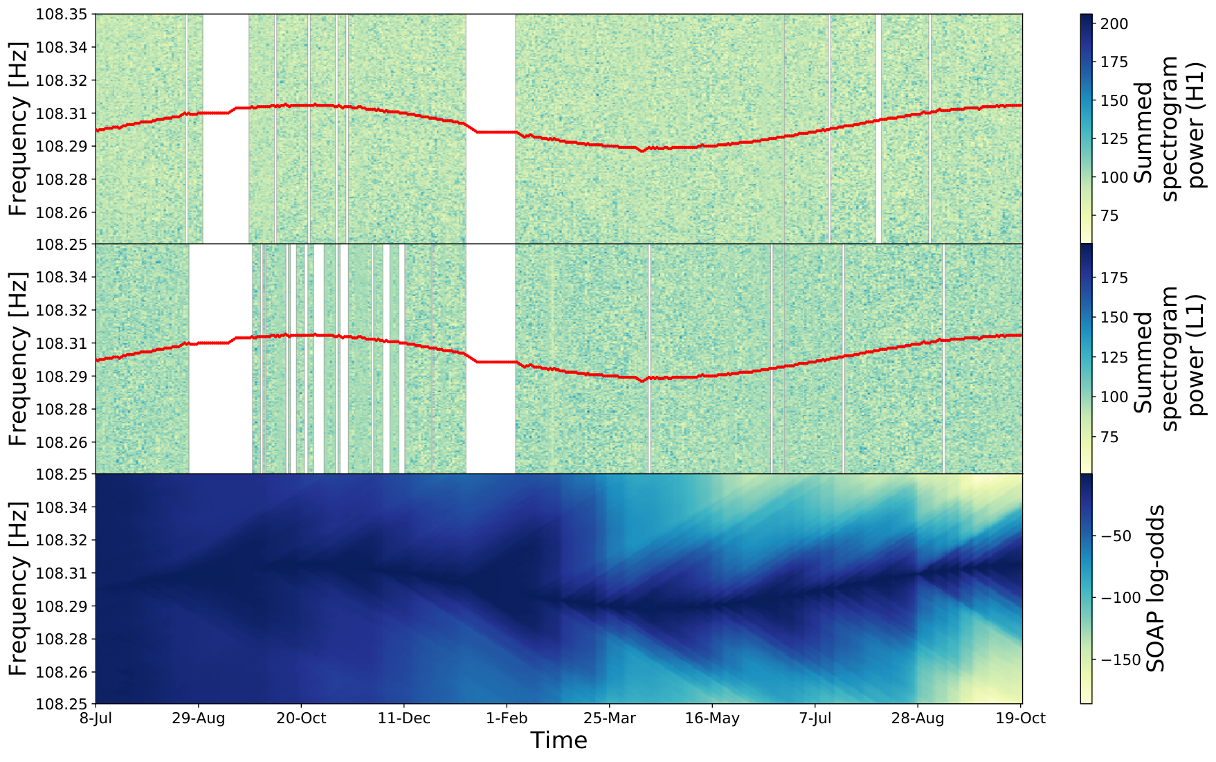
Refer to caption — Figure 1: An example of a SOAP search. The top two panels show time-frequency spectrograms, pre-processed according to Sec. V and representing a 0.1 Hz-wide frequency band from the LIGO S6 observing run. The data includes a simulated CW signal. The white areas in the spectrograms are gaps in data when the corresponding detector was not operating. The optimal track found by SOAP is overlaid in both cases. The bottom panel shows the normalised Viterbi map with the pixel intensity showing the log-probability that the track falls in a particular frequency bin as a function of time.

Viterbi track: The Viterbi track is the most probable track through time-frequency data for given a choice of statistic (i.e. summed SFT (SFT) power).
Viterbi statistic: The Viterbi statistic is the sum of the individual statistics along the Viterbi track. In the analysis that follows we use the ‘line-aware’ Viterbi statistic. This is the sum of the log-odds ratios, $p_{\rm signal}/(p_{\rm line}+p_{\rm noise})$ along the track Bayley et al. 2019.
Viterbi map: The Viterbi map shows the value of the Viterbi statistic for every time-frequency bin in the spectrogram, corresponding to the log-probability that the track passes through each time-frequency bin. Each time slice in the map is normalised individually, i.e., each vertical slice is adjusted so that the sum of their exponentiated values is unity. Each pixel in the image can therefore be interpreted as a value related to the log-probability that the signal is in that frequency bin at that time.

In Bayley et al. 2019 we used the Viterbi ‘line-aware’ statistic (described above) to determine whether the signal had an astrophysical origin. This statistic reduces the effect of instrumental lines on the analysis, but certain types of line are not picked-up by it. For example, the statistic is affected by broad, wandering, common lines as they offer high power tracks in both detectors. To reduce the effect of these instrumental lines in Bayley et al. 2019, we examined the spectrograms and Viterbi maps of individual bands by eye, as in Fig. 1. Bands which appeared to be contaminated were then manually removed from the search.

In this paper we show that we can exploit additional information in the spectrograms and Viterbi map, in combination with the Viterbi statistic, to perform the process of removing contaminated bands automatically . The tool which we use to classify this extra information is a convolutional neural network.

III Convolutional neural networks

CNN are a type of deep neural network which are primarily used in image processing and recognition Lecun et al. 2015; LeCun et al. 1998; Waibel et al. 1989; Krizhevsky et al. 2012. A CNN is designed to take in data, identify different features within that data and classify what those features or combinations of those features mean. In the context of this work the input data is a time-frequency spectrogram which may contain a (simulated) CW signal. The output is then a single number which represents the confidence that a signal is present. Values closer to 1 represent the presence of a signal and closer to 0 represent its absence. A CNN can learn how to identify features by training on many labelled examples of the input data where the output is known. For example, an input spectrogram with a CW signal would have a label of 1. Given the set of training examples, the many parameters of the CNN can be updated such that it gives the best result for any new spectrogram image. The many parameters of the CNN relate to the key building block of neural networks: the neuron.

III.1 Neurons

A neuron converts any number of inputs into a single output value and can perform three operations which are applied to $N$ inputs ${\bm{x}}$ : multiplying each input by a ‘weight’ $w$ , adding a ‘bias’ $b$ and passing them through, and applying a non-linear ‘activation function’ $f$ . Fig. 2 shows this basic operation, where there is one weight for every input and a single bias for each neuron. The output $O$ is therefore related to the inputs by

O=f\left(b+\sum_{i=1}^{N}w_{i}x_{i}\right).

(1)

The weights and bias are the parameters which the neural network ‘learns’ during training and we consider this further in Sec. III.4. The activation function is there to explicitly impose a non-linearity to the calculation.

Figure 2: Eq. 1 can be visualized as above. Here the inputs

x_{i}

are multiplied by the corresponding weights

w_{i}

, the sum of these and the bias

b

are then passed through an activation function

f

to the output. This example has four inputs but there can be any number.

III.2 Neural Networks

To create a neural network, many of these neurons are connected together into ‘layers’. Layers comprise a set of neurons, each of which takes the same data as input but which applies a different sets of weights and biases. The output of each neuron then acts as the input to another set of neurons or another layer. Neural networks combine many of these layers together to learn abstract representations of the data. For classification, this abstract representation is distilled down to a simple output. Neural networks can be made from many different types of layers. We described a ‘fully-connected’ layer above, in which each neuron in the layer takes in all the data points or the previous layer’s outputs. However for certain types of problem, such as identifying features in images, another type of layer called a convolutional layer is better suited.

III.3 Convolutional layers

Convolutional layers are an adaptation of the fully-connected layers described above in Sec. III.2, where the input data is generally image pixels. For this type of layer there is not a separate weight for each input data point (pixel). Rather, there is a fixed number of weights defined by a ‘filter’ size. This filter is convolved with the input image such that the output of the layer is a filtered image. This operation is shown in Fig. 3. The convolutional layers equivalent to Eq. 1 is,

O_{ij}=f\left(b+\sum_{m}\sum_{n}F_{mn}x_{i-m,j-n}\right),

(2)

where $O$ is the output image, $b$ is the bias, $x$ is the input image, $F$ is the convolutional filter and $f$ is the activation function. The indices $m$ and $n$ iterate over the filter rows and columns and the indices $i$ and $j$ iterate over the input image rows and columns. The convolutional layer can learn to identify features within an image by changing the weights and bias of a filter. A convolutional layer can apply a number of these filters as defined by the user. If the layer has 10 filters then the output is 10 filtered images. Each of these filters can then be trained to identify different features within the input image LeCun et al. 1998; Krizhevsky et al. 2012.

The output of a convolutional layer comprises a number of filtered images, so potentially there is a lot of data to feed to the next layer. A method called max-pooling can be used to reduce the size of the output whilst retaining the important information within the images. A max-pooling layer splits the image into blocks of fixed size and takes the maximum pixel value in each block as the output. So if the size of the max-pooling block is $2\times 2$ , the output image will have $1/4$ the number of pixels of the input.

Figure 3: The convolutional layers convolve a filter with the input image and output a convolved image the same size as the input to pass to the next layer. Here we show a simple

5\times 5

image with a

3\times 3

filter, the input is padded with zeros such that the output is the same size. When the network is trained, the values within the filter (the red values below the inputs) are updated.

III.4 Training

Once the structure of the network is decided, the network needs to be trained by adjusting the weights and biases to give the desired performance. To achieve this the networks classify the input images (the spectrograms and Viterbi maps) using a single output neuron with a sigmoid activation function which restricts the output between 0 and 1. The CNN is trained using a supervised learning process in which the class of each input example is known. We assign a label of 1 when the input is a time-frequency spectrogram which includes a simulated CW signal and 0 when there is no signal.

The performance of the network can be improved by increasing the number of input examples which is sees during training. This helps it learn the underlying features within the data and prevents it from over-fitting to specific examples.

Each of the training examples is then propagated though the network to its corresponding single output value, which lies between 0 and 1. This output is then compared to the label of the input data using a loss function. For our two-class network the loss function, $L$ , is the binary cross-entropy Goodfellow et al. 2016

L=-y\log{(p)}+(1-y)\log{(1-p)},

(3)

where $p$ is the network’s output, which has any value in the range $[0,1]$ and $y$ is the true output which has the binary label 0 or 1. The loss function is minimised when the output matches the truth. Its current value is used to train the network by updating the weights and biases through the process of ‘back-propagation’, typically using the derivative of the loss function with respect to a weight to update that weight Kingma and Ba 2015.

III.5 Network Structure

In this section we describe the structure of the networks used in our analysis. There are three possible inputs for each CNN: a spectrogram, a Viterbi map and the Viterbi statistic. Each of these are different representations of the raw detector data. We proceed by training a separate CNN for each input separately and then a further three CNN which use combinations of inputs: Viterbi map + spectrogram, Viterbi map + Viterbi statistic and Viterbi map + Viterbi statistic + spectrogram. With the exception of the output layer, all the CNN layers use the ‘leakyRELU’ activation function Maas 2013 in Eq. 2 and 1. We use a sigmoid activation function for the output neuron so that, for a given input, a CNN generates an output a value between 0 and 1. The closer this output value is to 1 the greater the probability that the input contains a signal, so this output value can then be treated as a detection statistic. The structure of the networks for the Viterbi map (vitmap), spectrograms and their combinations are shown in Fig. 4 and the components are described below:

Viterbi statistic: This is the simplest of the networks and comprises a single neuron which takes in the Viterbi statistic, applies a weight and bias and passes the result through a sigmoid function. This would give the same sensitivity as the Viterbi statistic on its own, however can now easily be combined with other networks.
Viterbi map: The Viterbi map CNN takes in a down-sampled Viterbi map of size (156,89) as input, described in Sec. IV.3. As shown in Fig. 4, this CNN consists of two convolutional layers and three fully-connected layers. The first layer has 8 filters which have a size of $5\times 5$ pixels, the second layer has 8 filters with a size of $3\times 3$ pixels. After each of these layers we use a max-pooling layer with a size of $8\times 8$ pixels. This is then passed into three fully-connected layers which all have 8 neurons and used leakyRELU activation functions. Finally these lead to an output neuron which uses a sigmoid activation function.
Spectrogram: The spectrogram CNN takes down-sampled spectrograms of size (156,89) as inputs (see Sec. IV.3). It has an identical structure to the Viterbi map CNN but takes the spectrograms of two different detectors as inputs.

The next three networks are constructed from combinations of these single CNN:

Viterbi map and spectrogram: To combine the spectrogram and Viterbi map network we remove the final output neuron and its 8 weights from each of the networks and combine these to a single sigmoid neuron with 16 new weights.
Viterbi map and Viterbi statistic: In this network we combine the Viterbi statistic with the Viterbi map. As before, this uses the pre-trained Viterbi map and Viterbi statistic CNN. Again, the output sigmoid neuron and corresponding weights are removed from each network. The 8 neurons from the Viterbi map network and the single neuron from the Viterbi statistic network are then combined to a single neuron with 9 new weights.
Viterbi map, Viterbi statistic and spectrogram: This combination takes all component CNN from above. As before the final sigmoid output and the corresponding weights from each network are removed. The 8 neurons from the Viterbi map and spectrograms CNN and the single neuron from the Viterbi statistic are then joined into a single output neuron with 17 new weights.

To combine CNN we use ‘transfer learning’ Pratt 1993by taking the pre-trained weights of the networks as a starting point for further training. In our examples we found that we could fix the weights inside the pre-trained networks and just train the final 16 output weights from the neurons as in Fig. 4. We chose to investigate combinations of networks because different representations of the data should contain slightly different information on the presence of a signal. For example, the Viterbi statistic contains no information on the structure of the track in the time-frequency plane, and the Viterbi maps lose some information about multiple lines in the band. The spectrograms contain the most information but in an unprocessed form. When used in combination, the resulting CNN should be able to pick the important features from each of these representations.

IV Data generation

To train the CNN we need to generate many examples of labelled data corresponding to the three data inputs used above, i.e., Time-frequency spectrograms, Viterbi maps and Viterbi statistics. The training data needs to include many examples of possible features which could appear, such as Gaussian noise, non-Gaussian artefacts and CW signals. Non-Gaussian artefacts are difficult to simulate, but it is possible to use artefacts in real data as part of the training set. Therefore, for the majority of the analysis that follows, the time-frequency spectrograms used to generate the Viterbi data come from real LIGO observing runs (see Sec. VI).

Overall, we need to consider three sets of data,, labelled ‘training data’, ‘test data’ and ‘search data’. Training data contains a set of augmented (see Sec. IV.2) time-frequency spectrograms containing simulated signals and is used to train each of the networks. Test data is a separate set of simulations which are not augmented. These are used to generate efficiency curves and test the network. Search data does not contain any simulated signal injections and is used to search for real signals within the data.

When training and testing a network it is important that the networks are not trained and tested on the same data. Otherwise the CNN can learn specific features of the training data and not the underlying distribution of features. To avoid this, the spectrograms are split into sub-bands of width $0.1$ Hz. Alternating bands are designated as ‘odd’ or ‘even’, so that bands starting at 100.1, 100.3 Hz are odd and those starting at 100.2, 100.4 Hz are even etc. The networks can then be trained on the odd bands and tested on the even bands and vice versa. When we search over data we will therefore have two trained networks, one for the even bands and one for the odd bands.

IV.1 Signal simulations

To inject simulated signals into real data we first generate a set of signals with parameters drawn randomly from prior distributions defined in Table 1. The SNR (SNR) of the simulations is uniformly distributed between 50 and 150. Where the SNR is the coherently ‘recovered’ SNR defined in Eq. 5. This is calculated for each time segment using the definition of optimal SNR in Prix 2007, the total SNR is then the sum of the squares of these. The GW amplitude $h_{0}$ is scaled based on the noise PSD (PSD) to achieve this SNR. The power spectrum of the signal can then be simulated in each time segment of a time-frequency spectrogram. This is done by assuming that the spectrogram is $\chi^{2}$ distributed. The the antenna pattern functions are taken into account for the given source parameters and detector such that the SNR for each time segment is calculated. This SNR is spread over neighbouring frequency bins dependent on its location in frequency. The power spectrum values can then be drawn from a non-central $\chi^{2}$ distribution with the non centrality parameter equal to the square of the SNR. Each signal is simulated in two detectors: LIGO H1 and L1. The SNR reported below are then the sum of the squares of the SNR from each detector. The simulation code used in this analysis can be found in Bayley 2020.

Table 1: The upper and lower limits bounding the random signal parameter. The parameters

\alpha,\sin{\left(\delta\right)},f,\;\log{\left(\dot{f}\right)},\;\cos{\left(\iota\right)},\;\phi_{0},\;\psi

were sampled uniformly between these ranges. The frequencies

f_{\rm l}

and

f_{\rm u}

refer to the lower and upper frequency of the band into which each signal is injected. Excluding the distribution of frequencies

f

, all the injections parameters are sampled from the same distributions as the S6 MDC Walsh et al. 2016.

	$\alpha$ [rad]	$\sin\left(\delta\right)$ [rad]	$f$ [Hz]	$\log_{10}\left(\dot{f}[\rm{Hz/s}]\right)$	$\cos{\iota}$ [rad]	$\phi$ [rad]	$\psi$ [rad]
lower bound	$0$	$-1$	$f_{\rm l}+0.25$	$-9$	$-1$	$0$	$0$
upper bound	$2\pi$	$1$	$f_{\rm u}-0.25$	$-16$	$1$	$2\pi$	$\pi/2$

IV.2 Augmentation

To train a neural network, many examples of data from each class are needed to avoid over-fitting. Simply using data between 40 and 500 Hz and splitting the data into 0.1 Hz wide sub-bands does not give enough data for the networks to be trained effectively. We therefore use the technique of data augmentation Patrice et al. 1991; Baird 1992 to artificially increase the number of training examples. Augmentation is the process of transforming existing data so that, to the network, it appears to be ‘new’ data. For example, by reversing a time-frequency band in time we get a new realisation of noise in that frequency band. This gives two noise realisations for each frequency band and would double the size of the training data-set, reducing the likelihood of over-fitting to the training data.

We applied augmentations to the spectrograms from each of the detectors. The augmentations that are used on each sub-band are: reversing the data in time, flipping the data in frequency, rolling the data in time by a small number of segments and shifting the data in frequency by a small number of bins. As we use real data, there are gaps in time where the detectors were not operating. We preserve the location of these gaps when augmenting the data. When shifting the data in frequency we shift each band up and down by 30 frequency bins (0.016 Hz) and up and down by 60 frequency bins (0.032 Hz). When rolling the data in time, we roll each sub-band by 100 time segments (100 days). Fig. 5 shows examples of the original data, a flip in frequency, a roll in time and a flip in time. For each frequency shift, we flip the sub-band in time and frequency and roll the sub-band in time. This then gives us three transformations for each of the four frequency shifts, which including the original data gives 15 augmentations of each band and therefore 15 times the number of training examples.

IV.3 Downsampling

The raw spectrograms contain a large number of pixels and, as the spectrograms pass through the network, there are a correspondingly large number of computations to perform and a significant burden on memory. To reduce their size, the spectrograms are binned in time over one day, i.e., every 48 time segments, as in Bayley et al. 2019. As well as reducing the size of the spectrogram, this increases the SNR within a given time-frequency bin assuming that the signal remains within the frequency bin for the majority of the time segment. To reduce the size of the data further we used the ‘resize’ package from scikit-image Van Der Walt et al. 2014 to interpolate and resize the summed spectrograms to 156 time segments by 89 frequency bins. This size was defined based on the summed spectrograms of the S6 data-set. This is $1/3$ the number of summed segments in time and $1/2$ the number in frequency. This down-sampling is applied to the spectrograms and Viterbi maps. In Bayley et al. 2019 we demonstrated that summing spectrograms can increase the speed and sensitivity of our search. When down-sampling the image, we found that reducing the amount of data had a small affect on the sensitivity of the CNN used.

V Search pipeline

The components described above were combined to form a single search pipeline with a flow diagram shown in Figure 6 We ran this pipeline in three modes, to train the CNN, test the search and run a search on real data. The elements of the flow diagram are described below:

Figure 6: The SOAP pipeline from start to finish. There are three main sections: Training (red), Testing (green) and Searching (grey) for both the odd and even bands. The blue sections surrounding these indicate that the same operation is applied to each of the training, test and search data. The blue sections mean that the same operations are applied to all data in that section, for example, injections are made into training, test and search data for both odd and even bands in step 5.

1. SFTs: These are 1 800 s SFT generated from the detector strain time-series data. This is the standard SFT length for a number of CW searches.
2. Normalising: The SFT are then divided by their running median with a window width of 100 frequency bins. If we assume the resulting SFT to be $\chi^{2}$ distributed, we can apply a correction factor using LALSuite code XLALSFTtoRngmed LIGO Scientific Collaboration 2018 such that their power spectrum has a mean of $\sim 1$ . By then multiplying this by 2, the noise-like component of the spectrum is distributed as expected.
3. Narrowbanding: The computational efficiency can be improved if the data is divided into frequency bands so the analysis can be completed on each band using separate CPU nodes. In this search the spectrograms are split into $2.1$ Hz-wide bands every $2$ Hz, i.e. 100.0 to 102.1 Hz, 102.0 to 104.1 Hz etc. The analysis on each node will further split the data into 0.1 Hz wide sub-bands. The overlap then allow the sub-band from 1.95-2.05 to be calculated on one node. The band size was chosen based on the available computational memory at the time.
4. Band splitting: A CNN should not be trained on the same data that it will be tested on, so each of the $0.1$ Hz wide sub-bands are split into ‘odd’ or ‘even’ bands. A CNN can then be trained on even bands and tested on odd bands, and vice versa.
5a. Training data generation: The training data generation is described in Sec. IV. Each of the $0.1$ Hz sub-bands is ‘augmented’ (Sec. IV.2). For each of the augmented bands, the data is duplicated and signals are injected into the copy with SNR in the range 50-150 to give an example of a noise class member and a signal class member. There are two of these sets, one for ‘even’ bands and one for ‘odd’.
5b. Testing data generation: The signals in the testing data followin the parameters in Tab. 1 are injected in to 50% of the $0.1$ Hz sub-bands. These signals have an SNR in the range 20-200. The SNR range here is wider than the training set to show how the trained networks perform on this wider range. Again we have a set for ‘odd’ and a set for ‘even’ sub-bands.
5c. Search data: This data is generated to assess the performance of the trained network with real signals. The sub-bands described in part 4 are now overlapping by 0.05 Hz. This means that if there is an astrophysical signal it should be fully contained within at least one sub-band. We do assume that the signal frequency does not change by more than 0.1 Hz over a year, which is reasonable for isolated neutrons stars $<500$ Hz. There are both ‘odd’ and ‘even’ versions of this search data.
6. Summing spectrogram: Following the practice in Bayley et al. 2019 the spectrograms are summed over one day, i.e., we sum 48 contiguous 30-minute time segments of the spectrogram to give one time segment per day. This is done separately for each of the six data-sets (three for ‘odd’, three for ‘even’).
7. Generate lookup tables and run SOAP search: When the SOAP search is run using the line-aware statistic, lookup tables which contain values of the statistic as a function of the spectrogram power in each detector Bayley et al. 2019 are used to increase the speed of the analysis. These lookup tables are generated in advance of the search. Once done, we run separate SOAP search for each of the six data-sets (three ‘odd’, three ‘even’) separately.
8. Down-sample data: At this stage there are four saved elements for each of the six data-sets: two spectrograms, the Viterbi map and the Viterbi statistic. The spectrograms and the Viterbi map are down-sampled to a size of ( $156\times 89$ ) using interpolation from scikit-image’s resize Van Der Walt et al. 2014. This size was chosen based on the S6 MDC data-set, where this is 1/3 the length in time and 1/2 the width in frequency of the summed spectrograms. This was chosen such that the CNN trained efficiently and still achieved a reasonable sensitivity.
9. Train networks: The down-sampled training data is then used to train the CNN. One CNN is trained on ‘odd’ bands and another CNN with the same structure is trained on ‘even’ bands.
10b. Run search on testing data: The trained CNN from part 9 are then used to classify each sub-band in the testing data with injections. This returns a statistic in the range $[0,1]$ , where values closer to one imply that an astrophysical signal is likely to be present in the data. Here the CNN trained on the ‘odd’ bands is tested using the ‘even’ bands and vice versa. The algorithms are run on this test data to asses the sensitivity of the analysis.
10c. Run search on real data: The trained CNN from part 9 are then used to classify each sub-band in the search data, returning a statistic in $[0,1]$ as in part 10b. Once again the CNN trained on the ‘odd’ bands is run on the ‘even’ bands and vice versa.
11a. Signal candidates: The sub-bands which return a statistic in the top 1% of all sub-bands can be taken as potential candidates. This can then be followed-up with other CW search methods.
11c. Efficiency curves: The output statistics from the test data-set (11b.) are examined to assess how well the network has classified signals as a function of the injected signal SNR. A range of efficiency curves are generated, as detailed in Sec. VI.1.

VI Results

The networks described in Sec. III.5 were trained and tested on four different data-sets: the S6 MDC as in Bayley et al. 2019; Walsh et al. 2016, our own injections into O2 data, Gaussian noise with the same time gaps and noise floor as the S6 data-set, and our own injections into real S6 data. Each of the searches uses training and testing data in the frequency range of 100-400 Hz, except the S6 MDC which uses data in the range 40-500 Hz for consistency with other searches in the challenge. All of the networks were trained using the Adam optimiser Kingma and Ba 2015 with a learning rate of 0.001. For each training epoch the training data was split into random batches of size 1000, where the network weights are updated after each batch. The networks were trained for 400, 200 and 4000 epochs for the vitstat, vitmap and spectrogram networks respectively.

VI.1 Sensitivity

To investigate the sensitivity of the pipeline we use two measures: the sensitivity depth $\mathcal{D}$ Prix 2007 and the optimal SNR $\rho$ Behnke et al. 2015, both described in Bayley et al. 2019. The sensitivity depth is defined as

\mathcal{D}(f)=\frac{\sqrt{S_{h}(f)}}{h_{0}},

(4)

where $S_{h}(f)$ is the single-sided noise PSD and $h_{0}$ is the GW amplitude. The optimal SNR is defined as

\rho^{2}=\sum_{X}4\Re\int^{\infty}_{0}\frac{\tilde{h}^{X}(f)\tilde{h}^{X*}(f)}{S^{X}(f)}df,

(5)

where $X$ indexes over detectors and $\tilde{h}(f)$ is the Fourier transform of the time series of the signal $h(t)$ . $\rho^{2}$ is defined in Prix 2007 for a double-sided PSD but here we have defined it for the more common single-sided case.

The sensitivity curves shown in Fig. 8,9 and 10 were generated using a $1\%$ false alarm probability, which we use to set our detection threshold. This threshold is the statistic value exceeded by just $1\%$ of sub-bands that do not contain an injection. The efficiency is defined as the fraction of events which exceed the false alarm threshold for any given SNR. The SNR is sampled uniformly between the range 20-200 as described in Sec. V. Instead of having multiple simulations for a discrete set of SNR we define a window around a point in SNR and count the fraction of statistics which exceed the threshold determined by the false alarm probability within that window. We define the window as a Gaussian with a standard deviation of 2, which is wide enough to contain enough injections at a given SNR to return a reliable value. The detection efficiency $y(\rho)$ is

y(\rho)=\frac{\sum_{i}H(O_{i}-O^{1\%})\mathcal{G}(\rho_{i};\mu=\rho,\sigma=2)}{\sum_{i}\mathcal{G}(\rho_{i};\mu=\rho,\sigma=2)},

(6)

where $O_{i}$ is the output statistic from the CNN, $O^{1\%}$ is the statistic value corresponding to a 1% false alarm probability, $H$ is the Heaviside step function which has a value of 1 for positive input arguments and 0 for negative arguments. The SNR of a simulation with output $O_{i}$ is defined in Eq. 6 using $\rho_{i}$ . The centre of the window in SNR is then $\rho$ . The window is a Gaussian with a mean of the current SNR and a standard deviation of 2, $\mathcal{G}(\rho_{i},\mu=\rho,\sigma=2)$ . The sensitivity curves for each of the described data-sets are shown in Figs. 8,9 and 10.

For the first test, injections were made into the O2 data-set as described in Sec. IV between 100 Hz and 400 Hz. Each of the six networks described in Sec. III.5 were then trained and tested on this data. Fig. 7 shows an example of the training and validation loss and detection probability as a function of training epoch for the vitmap network trained on simulations in O2 data. One epoch is when the entire training set has been passed through the network. Fig. 7 shows that for both the training and an independent validation set, the loss and detection probability both converge and perform similarly on each data-set, implying that the network does not over-fit.

Figure 7: The loss and detection probability for training and validation sets as a function of training epoch for the vitmap network in the O2 data set. The loss decreases for both datasets with each epoch where the validation set converges after

\sim 100

training epochs. The detection probability is calculated as the fraction of all signal simulations which exceed the 1% false alarm value.

Figure 8 shows the sensitivity curves for the tests in O2 for both SNR and sensitivity depth for each of the six networks. Focusing on Fig. 8a, the least sensitive of the CNN is the Viterbi statistic (vitstat), and this is expected. We know that, despite the line-aware component to the Viterbi statistic calculation, it can still fail to distinguish between some instrumental lines and astrophysical signals. The spectrogram CNN has an improved sensitivity over the Viterbi statistic; this importantly does not involve the SOAP search but is run entirely on down-sampled and summed spectrograms. This network is approaching the most sensitive of the examples in Fig. 8. The difference in sensitivity between the spectrogram and the Viterbi map CNN is most likely due to the Viterbi map providing a distilled representation of the spectrograms which is easier for a CNN to interpret. It is possible that the spectrogram CNN could reach the same sensitivity as the Viterbi map CNN by changing its structure or the data-set resolution. However, as explained in more detail in Sec. VI.2, this network takes $\sim 10$ times longer to train than the Viterbi map network.

The remaining four networks contain the Viterbi map (vitmap) as one of their inputs (or their only input) and all achieve similar sensitivities. It appears therefore that the dominant effect on sensitivity is from the Viterbi maps component. In the following tests our focus will be on the Viterbi map CNN as in all cases this is competitively the most sensitive. For the O2 data-set we show that, with a false alarm probability of 1%, the Viterbi map CNN achieves a sensitivity of SNR $~95$ and sensitivity depth of $~12\;{\rm Hz}^{-1/2}$ with 95% efficiency. In Fig. 8a the sensitivity of the spectrogram CNN drops after an SNR of 150. This is most likely due to the training set containing simulations between and SNR of 50 and 150, and therefore has not seen signal simulations of higher SNR. The dip in sensitivity in Fig. 8b at lower depths is due to the same effect.

(a)

(b)

Figure 8: Tests of the six CNN with the O2 data-set between 100-400 Hz. The efficiency plots above are for a 1% false alarm probabilities. Fig. 8a shows the efficiency of the search as a function of SNR and Fig.8b shows the efficiency as a function of sensitivity depth. The efficiency here is a measure of the fraction of events which exceed the 1% false alarm probability for any given SNR. These plots both show that the sensitivity of the Viterbi statistic is significantly below that of the different CNN. The others group with a similar sensitivity.

For the second test we simulate the S6 data-set with Gaussian noise, retaining the same gaps in the data present in S6 but without including instrumental artefacts such as lines. The noise floor of S6 was also replicated by scaling the SNR of each injection by an estimate of the PSD at that frequency. Figure 9 shows the SNR and depth sensitivity curves for the Viterbi statistic and Viterbi map CNN for both the Gaussian noise run with S6 gaps and for injections into the real S6 data-set. In the Gaussian noise data-set the curves for both the Viterbi map CNN and the Viterbi statistic, show very similar results. This is to be expected as the main use of the CNN was to reduce the effect of instrumental lines, and there are none in this data set. The advantage of using the Viterbi maps in a CNN becomes clear when it is tested on simulations into real S6 data with many instrumental lines. The two curves corresponding to simulations in real S6 data in Fig. 9a show the sensitivity as a function of SNR in these tests. It becomes clear that the Viterbi map CNN reduces the effect of instrumental lines and increases the searches sensitivity to SNR. A similar feature can be seen in Fig.9b where the use of an CNN again greatly improves sensitivity.

These tests on S6 data also show that the effect of instrumental lines was far greater in this run than in O2. This is shown in Fig. 8a where the separation between the Viterbi statistic curves and the Viterbi map curves is significantly smaller than the S6 curves in Fig. 9a. For simulations into Gaussian noise following S6 gaps we show that with a false alarm of 1% the Viterbi map CNN achieves a sensitivity of SNR $~85$ and sensitivity depth of $~20\;{\rm Hz}^{-1/2}$ with 95% efficiency. For injections into real S6 data the search achieves a sensitivity of SNR $~115$ and sensitivity depth of $~11\;{\rm Hz}^{-1/2}$ with 95% efficiency and 1% false alarm. We can also see from Fig. 9a that the sensitivity of the vitmap CNN in Gaussian noise with S6 gaps is better than in real S6 data.

(a)

(b)

Figure 9: The sensitivity of the search for simulations in real S6 data (s6) compared to simulations in Gaussian noise (gauss) between 100-400 Hz. Figure 9a shows the efficiency of the search as a function of SNR and Fig. 9b shows the efficiency as a function of sensitivity depth. The efficiency is the fraction of events which exceed the 1% false alarm threshold for a given SNR or depth. The Gaussian noise injections included the same gaps in data as the S6 data set and the SNR of the simulated signal in Gaussian noise was adjusted to replicate the expected SNR in S6 data. In the Gaussian noise simulations the searches achieve an efficiency of

95\%

with 1% false alarm at an SNR

\sim 85

and

\sim 90

for the Viterbi map and Viterbi statistic respectively. In the real S6 noise simulations the searches achieve an efficiency of

95\%

with 1% false alarm at an SNR

\sim 108

and

>200

for the Viterbi map and Viterbi statistic respectively.

The final test also uses the S6 data-set, however, in this case we use the standard set of injections used in previous CW analysis pipeline comparisonsMDC Walsh et al. 2016. Fig. 10 shows the resultant sensitivity curves derived from these injections. In both Fig. 10a and 10b the sensitivity curves are substantially more noisy than in Fig. 8 or 9, mainly due to the smaller size of the testing set. The standard set of simulations in Fig. 10 contained $\sim 900$ signal simulations between 40 and 500 Hz where the majority of these signals are distributed between an SNR of 0 and 150. Figures 8 and 9 are generated using $2\,300$ simulations between 40 and 500 Hz and SNR of 20 and 200 as described in Sec. V. Figure 10b shows the direct comparison in depth of the results in Walsh et al. 2016 with the results from the SOAP search with the Viterbi map CNN. This shows that we achieve a sensitivity consistent with that of other semi-coherent searches with the exception of the Einstein@home search Abbott et al. 2016b. Whilst we are not the most sensitive search by this measure, the SOAP + CNN search offers a greatly reduced computational cost (see Sec. VI.2).

This particular test was limited to signals from isolated neutron stars. However, unlike some other semi-coherent searches, SOAP is sensitive to a broad range of continuous-wave signals, including binary sources and sources with limited coherence times. The inclusion of the CNN does introduce some dependency on the signal model, as the training set for the CNN contains simulations of isolated neutron stars. However, this is not a limitation of the method: new training sets can be readily generated using a different signal models. For tests in the S6 MDC we show that with a false alarm of 1% the Viterbi map CNN achieves a sensitivity in SNR of $\sim 110$ and sensitivity depth of $\sim 10\;{\rm Hz}^{-1/2}$ with 95% efficiency.

(a)

(b)

Figure 10: A comparison of the SOAP + CNN search with other CW searches through a standard set of injections used in the S6 MDC Walsh et al. 2016. We have taken the published list of detected sources for each search Walsh et al. 2016 and replotted using the method in Sec. VI.1 to compare the sensitivities to the SOAP + CNN search. This includes results for all source simulations between 40 and 500 Hz. The efficiency curves are generated with a 1% false alarm probability. The curves are substantially more noisy than in Fig. 8 or 9 as there is a smaller number simulations in a given SNR range.

VI.2 Computational time

A key parameter for any CW search is the computational time it takes to run. Table 2 shows the timings for different sections of the search using the S6 data-set. This is split into three sections: data generation, CNN training and CNN testing. The majority of the computational time taken to get from raw SFT to results occurs is the data generation step. The timings shown Tab. 2 are for the S6 observing run where each section is run on a single CPU (CPU) or GPU (GPU), however, in practice the generation of the data is run on multiple CPU on a computing cluster. The training and testing of a CNN is done on a single GPU, this substantially decreases the training time compared to a CPU due to the intrinsically parallel nature of neural networks.

Table 2: Approximate timings for training and testing using the S6 data-set (the longest run we tested), starting from 22 538 SFT each of duration 1 800 s. The frequency range covered is 40-500 Hz. In the training, testing and search data sections we averaged the SFT over one day to give 469 time segments as input to the CNN. The data generation times quoted are for a single CPU however, in reality this will be split across many separate CPU. The training and testing is completed on a single GPU.

Generating data on single CPU
	Time [hrs]
Narrow-banding	$\sim 9$
Training data	$\sim 240$
Testing data	$\sim 75$
Search data	$\sim 40$
Training CNN on single GPU
	Training time [hrs]	Loading time [hrs]
Viterbi statistic	$0.03$	$0.2$
Viterbi map	$0.8$	$0.7$
spectrogram	$9$	$1$
Viterbi map
+ Viterbi statistic	$1$	$0.7$
Viterbi map
+ spectrogram	$1.4$	$1.6$
Viterbi map
+ Viterbi statistic
+ spectrogram	$1.5$	$2$
Testing CNN on real data on GPU
	Testing [s]	Loading [s]
All CNN	$5$	$60-160$

Starting with raw SFT covering the 40-500 Hz band of the S6 data-set (i.e., 22 538 time segments each 1 800 s long, giving 828 000 frequency bins in total) and without any trained networks, this search would have a total computing time of $\sim 386$ hours on a single CPU and GPU. However, the majority of this time is used making the simulated data. The generation of training, testing and search data can be easily parallelised, and in practice this is split over 200 CPU and takes just $\sim 2$ real-time hours ( $\sim 355$ CPU hours). After this parallelisation, if one was given S6 data without any trained networks, the search would then take approximately $13$ hours to get an efficiency curve and a list of candidates. In this case I assume that only the Viterbi map network is trained and tested based on the conclusions from Sec. VI.

The computational cost can be reduced further if a network has been trained on a previous observing run, negating the need for new training data and the training itself. This reduces the total run time on S6 to $\sim 9.5$ hours (on 200 CPU). The reduction is significant but not drastic, as the majority of the time is spent narrow-banding the SFT.

To reduce the time taken to generate results at the end of an observing run, one could narrowband the SFT periodically as the data is taken during an observing run. This would allow the results to be generated within $\sim 3.5$ hours of the end of the run. SFT generated on a regular basis would allow results to be generated during an observing run. This could be done, for example, on a weekly basis by adding 7 days of pixels to a spectrogram, then retraining a CNN and generating results.

The computational cost of this search is small when compared to other existing CW searches. In Walsh et al. 2016 the expected computational cost for the first 4 months of O1 for each search is shown, where the fastest search takes $0.9$ million core-hours (Hough searches) and the slowest is $100-170$ million core-hours (Einstein@Home). The equivalent cost of the SOAP + CNN search is $\sim 100-200$ core-hours which is $\sim 5-10$ thousand times faster.

VII Summary

In this paper we summarise an extension of the SOAP algorithm (Bayley et al. 2019). The extension makes use of a CNN to limit the effect of instrumental lines in searches for astrophysical CW signals. The SOAP search has a number of outputs and in this paper we focussed on two of these: the Viterbi statistic and the Viterbi map. The Viterbi statistic has previously been used as a measure of whether a given frequency band contains an astrophysical signal (Bayley et al. 2019). The Viterbi map is an output map with the same shape as the input spectrogram, with a value related to the probability that a signal passes through any particular time-frequency bin. We use both the Viterbi map and spectrogram as input images to a CNN and classify each frequency band as containing an astrophysical signal or not. This approach removes then need to manually look through frequency bands and remove those which are contaminated with non-astrophysical (instrumental) features.

In detail, we tested six separate CNN which take in a combination of three representations of the input data: the Viterbi statistic, the Viterbi map and a normalised spectrogram. The objective here was to combine these different representations of the data to increase the robustness and sensitivity of the search. The tests found that the CNN which uses the Viterbi map alone as input was more sensitive than any other which used a single data type as input. Each of the CNN that used a combination of input data types had a similar sensitivity to the Viterbi map CNN. Therefore we concluded that the Viterbi map provides the most useful summary of information for detecting a signal. Given that the main aim of this investigation was to reduce the effect of instrumental lines on the SOAP search, it is unsurprising that tests with Gaussian noise data (with no such lines) showed the CNN search achieved a similar sensitivity to the Viterbi statistic alone. The tests in Gaussian noise with S6 gaps showed that at a 95 % efficiency and a 1% false alarm probability the Viterbi statistic and Viterbi map achieved a sensitivity of SNR 95 and 90 respectively. When the same test was run in real S6 data at a 95 % efficiency and a 1% false alarm probability the Viterbi statistic and Viterbi map achieved corresponding sensitivities of SNR 300 and 120 respectively. This demonstrates that the CNN approach adds robustness to SOAP and regains much of the sensitivity that would otherwise be lost to the effects of instrumental lines in real detector data.

These tests were repeated using a standard set of injections into S6 data to make a direct comparison with other CW search pipelines. At a 95% efficiency and a 1% false alarm probability the Viterbi map CNN achieved a sensitivity of SNR $\sim 110$ and a sensitivity depth $\sim 10\;\rm{Hz}^{-1/2}$ . We have shown that the SOAP + CNN approach can achieve a similar sensitivity to other semi-coherent CW search algorithms but with a greatly reduced computational cost.

This search also offers significant flexibility in the type of signal that is searched for. In the above examples the focus is on isolated neutron stars, largely to make a straight comparison with other CW searches that are tuned for these sources. However, the search framework itself is largely model-free and non-parametric. By changing the training sets, the same pipeline can be optimised for different signal types, and in future work we aim to test its ability to identify other sources of GW such as neutron stars in binary systems. Additionally, we will apply a more advanced Bayesian analysis to estimate basic source parameters which would then provide crucial information for a more sensitive search by fully-coherent pipelines.

VIII Acknowledgements

We would like to acknowledge the continuous wave working group of LIGO-Virgo Collaboration for their assistance during this project. We would also like to acknowledge Sinéad Walsh for providing us with the data from the S6 MDC paper. This research is supported by the Science and Technology Facilities Council., J.B. G.W. and C.M. are supported by the Science and Technology Research Council (grant No. ST/L000946/1). C.M. is also supported by the European Cooperation in Science and Technology (COST) action CA17137. The authors are grateful for computational resources provided by the LIGO Laboratory supported by National Science Foundation Grants PHY-0757058 and PHY-0823459.

References

Bayley et al. (2019) J. Bayley, G. Woan, and C. Messenger (2019), eprint 1903.12614, URL http://arxiv.org/abs/1903.12614http://dx.doi.org/10.1103/PhysRevD.100.023006.
Walsh et al. (2016) S. Walsh, M. Pitkin, M. Oliver, S. D’Antonio, V. Dergachev, A. Królak, P. Astone, M. Bejger, M. Di Giovanni, O. Dorosh, et al., Phys. Rev. D 94, 124010 (2016), ISSN 24700029, eprint 1606.00660, URL https://link.aps.org/doi/10.1103/PhysRevD.94.124010.
Abbott et al. (2009) B. P. Abbott, R. Abbott, R. Adhikari, P. Ajith, B. Allen, G. Allen, R. S. Amin, S. B. Anderson, W. G. Anderson, M. A. Arain, et al., Reports Prog. Phys. 72, 076901 (2009), ISSN 00344885, eprint 0711.3041, URL http://stacks.iop.org/0034-4885/72/i=7/a=076901?key=crossref.669f7c34d7d28503fd7f84b53db6048f.
Aasi et al. (2015) J. Aasi, B. P. Abbott, R. Abbott, T. Abbott, M. R. Abernathy, K. Ackley, C. Adams, T. Adams, P. Addesso, R. X. Adhikari, et al., Class. Quantum Gravity 32, 074001 (2015), ISSN 13616382, eprint 1411.4547, URL http://stacks.iop.org/0264-9381/32/i=7/a=074001?key=crossref.20895763c84bce3f8929251031b2475c.
Acernese et al. (2015) F. Acernese, M. Agathos, K. Agatsuma, D. Aisa, N. Allemandou, A. Allocca, J. Amarni, P. Astone, G. Balestri, G. Ballardin, et al., Class. Quantum Gravity 32, 024001 (2015), ISSN 13616382, URL http://stacks.iop.org/0264-9381/32/i=2/a=024001?key=crossref.f3779cf21eab5f6631c6650a20708030.
Acernese et al. (2008) F. Acernese, M. Alshourbagy, P. Amico, F. Antonucci, S. Aoudia, P. Astone, S. Avino, L. Baggio, G. Ballardin, F. Barone, et al., Class. Quantum Gravity 25, 114045 (2008), ISSN 02649381, URL http://stacks.iop.org/0264-9381/25/i=11/a=114045?key=crossref.62c81a5e3c6d5978d66477c5fb155f0c.
Abbott et al. (2017a) B. P. P. Abbott, R. Abbott, T. D. D. Abbott, F. Acernese, K. Ackley, C. Adams, T. Adams, P. Addesso, R. X. X. Adhikari, V. B. B. Adya, et al., Phys. Rev. Lett. 119, 161101 (2017a), ISSN 10797114, URL https://link.aps.org/doi/10.1103/PhysRevLett.119.161101.
Abbott et al. (2017b) B. P. P. Abbott, R. Abbott, T. D. D. Abbott, F. Acernese, K. Ackley, C. Adams, T. Adams, P. Addesso, R. X. X. Adhikari, V. B. B. Adya, et al., Phys. Rev. Lett. 119, 141101 (2017b), ISSN 10797114, URL https://link.aps.org/doi/10.1103/PhysRevLett.119.141101.
Abbott et al. (2016a) B. P. Abbott, R. Abbott, T. D. Abbott, M. R. Abernathy, F. Acernese, K. Ackley, C. Adams, T. Adams, P. Addesso, R. X. Adhikari, et al., Phys. Rev. Lett. 116, 061102 (2016a), ISSN 10797114, URL https://link.aps.org/doi/10.1103/PhysRevLett.116.061102.
Prix (2009) R. Prix, in Neutron Stars Pulsars (Springer Berlin Heidelberg, Berlin, Heidelberg, 2009), pp. 651–685, URL http://link.springer.com/10.1007/978-3-540-76965-1_24.
Dupuis and Woan (2005) R. J. Dupuis and G. Woan, Phys. Rev. D - Part. Fields, Gravit. Cosmol. 72, 102002 (2005), ISSN 15507998, URL https://link.aps.org/doi/10.1103/PhysRevD.72.102002.
Schutz (1998) B. Schutz, Phys. Rev. D - Part. Fields, Gravit. Cosmol. 58, 063001 (1998), ISSN 15502368.
Abbott et al. (2019) B. P. Abbott, R. Abbott, T. D. Abbott, S. Abraham, F. Acernese, K. Ackley, C. Adams, R. X. Adhikari, V. B. Adya, C. Affeldt, et al. (LIGO Scientific, Virgo), Phys. Rev. D 100, 024004 (2019), ISSN 2470-0010, eprint 1903.01901, URL https://link.aps.org/doi/10.1103/PhysRevD.100.024004.
Creighton (2000) T. Creighton, Phys. Rev. D - Part. Fields, Gravit. Cosmol. 61, 082001 (2000), ISSN 15502368, URL https://link.aps.org/doi/10.1103/PhysRevD.61.082001.
Riles (2017) K. Riles (2017), eprint 1712.05897v1.
Sieniawska and Bejger (2019) M. Sieniawska and M. Bejger, Universe 5, 217 (2019), URL https://www.mdpi.com/2218-1997/5/11/217.
Bayley (2020) J. C. Bayley, Soapcw (2020), URL https://git.ligo.org/joseph.bayley/soapcw.
Covas et al. (2018) P. B. Covas, A. Effler, E. Goetz, P. M. Meyers, A. Neunzert, M. Oliver, B. L. Pearlstone, V. J. Roma, R. M. Schofield, V. B. Adya, et al. (LSC Instrument Authors), Phys. Rev. D 97, 082002 (2018), ISSN 24700029, eprint 1801.07204.
Keitel et al. (2014) D. Keitel, R. Prix, M. A. Papa, P. Leaci, and M. Siddiqi, Phys. Rev. D 89, 064023 (2014), URL https://link.aps.org/doi/10.1103/PhysRevD.89.064023.
Leaci (2015) P. Leaci, Phys. Scr. 90, 125001 (2015), ISSN 1402-4896, URL https://doi.org/10.1088%2F0031-8949%2F90%2F12%2F125001.
Zhu et al. (2017) S. J. Zhu, M. A. Papa, and S. Walsh, Phys. Rev. D 96, 124007 (2017), URL https://link.aps.org/doi/10.1103/PhysRevD.96.124007.
Gabbard et al. (2018) H. Gabbard, M. Williams, F. Hayes, and C. Messenger, Phys. Rev. Lett. 120, 141103 (2018), ISSN 10797114, URL https://link.aps.org/doi/10.1103/PhysRevLett.120.141103.
George and Huerta (2018) D. George and E. A. Huerta, Phys. Lett. Sect. B Nucl. Elem. Part. High-Energy Phys. 778, 64 (2018), ISSN 03702693, URL https://www.sciencedirect.com/science/article/pii/S0370269317310390?via%3Dihub.
Gebhard et al. (2019) T. D. Gebhard, N. Kilbertus, I. Harry, and B. Schölkopf, Phys. Rev. D 100, 063015 (2019), ISSN 24700029, URL https://link.aps.org/doi/10.1103/PhysRevD.100.063015.
Chan et al. (2019) M. L. Chan, I. S. Heng, and C. Messenger, arXiv:1912.13517 [astro-ph] (2019), eprint 1912.13517, URL http://arxiv.org/abs/1912.13517.
Iess et al. (2020) A. Iess, E. Cuoco, F. Morawski, and J. Powell, Mach. Learn.: Sci. Technol. 1, 025014 (2020), ISSN 2632-2153, URL https://doi.org/10.1088%2F2632-2153%2Fab7d31.
Astone et al. (2018) P. Astone, P. Cerdá-Durán, I. Di Palma, M. Drago, F. Muciaccia, C. Palomba, and F. Ricci, Phys. Rev. D 98, 122002 (2018), URL https://link.aps.org/doi/10.1103/PhysRevD.98.122002.
Dreissigacker et al. (2019) C. Dreissigacker, R. Sharma, C. Messenger, R. Zhao, and R. Prix, Phys. Rev. D 100, 044009 (2019), ISSN 24700029, URL https://link.aps.org/doi/10.1103/PhysRevD.100.044009.
Miller et al. (2019) A. L. Miller, P. Astone, S. D’Antonio, S. Frasca, G. Intini, I. La Rosa, P. Leaci, S. Mastrogiovanni, F. Muciaccia, A. Mitidis, et al., Phys. Rev. D 100, 062005 (2019), URL https://link.aps.org/doi/10.1103/PhysRevD.100.062005.
Morawski et al. (2020) F. Morawski, M. Bejger, and P. Ciecieląg, Mach. Learn.: Sci. Technol. 1, 025016 (2020), ISSN 2632-2153, URL https://doi.org/10.1088%2F2632-2153%2Fab86c7.
Cuoco et al. (2020) E. Cuoco, J. Powell, M. Cavaglià, K. Ackley, M. Bejger, C. Chatterjee, M. Coughlin, S. Coughlin, P. Easter, R. Essick, et al., arXiv:2005.03745 [astro-ph, physics:gr-qc] (2020), eprint 2005.03745, URL http://arxiv.org/abs/2005.03745.
Viterbi (1967) A. J. Viterbi, IEEE Trans. Inf. Theory 13, 260 (1967), ISSN 15579654, URL http://ieeexplore.ieee.org/document/1054010/.
Lecun et al. (2015) Y. Lecun, Y. Bengio, and G. Hinton, Nature 521, 436 (2015), ISSN 14764687, URL http://www.nature.com/articles/nature14539.
LeCun et al. (1998) Y. LeCun, L. Bottou, Y. Bengio, and P. Haffner, Proc. IEEE 86, 2278 (1998), ISSN 00189219, URL http://ieeexplore.ieee.org/document/726791/.
Waibel et al. (1989) A. Waibel, T. Hanazawa, G. Hinton, K. Shikano, and K. J. Lang, IEEE Trans. Acoust. 37, 328 (1989), ISSN 00963518, URL http://ieeexplore.ieee.org/document/21701/.
Krizhevsky et al. (2012) A. Krizhevsky, I. Sutskever, and G. E. Hinton, in Advances in Neural Information Processing Systems 25, edited by F. Pereira, C. J. C. Burges, L. Bottou, and K. Q. Weinberger (Curran Associates, Inc., 2012), pp. 1097–1105, URL http://papers.nips.cc/paper/4824-imagenet-classification-with-deep-convolutional-neural-networks.pdf.
Goodfellow et al. (2016) I. Goodfellow, Y. Bengio, and A. Courville, Deep Learning (MIT Press, 2016).
Kingma and Ba (2015) D. P. Kingma and J. L. Ba, 3rd Int. Conf. Learn. Represent. ICLR 2015 - Conf. Track Proc. (2015), eprint 1412.6980, URL http://arxiv.org/abs/1412.6980.
Maas (2013) A. L. Maas, Rectifier Nonlinearities Improve Neural Network Acoustic Models (2013), URL /paper/Rectifier-Nonlinearities-Improve-Neural-Network-Maas/367f2c63a6f6a10b3b64b8729d601e69337ee3cc.
Pratt (1993) L. Y. Pratt, in Advances in Neural Information Processing Systems 5, edited by S. J. Hanson, J. D. Cowan, and C. L. Giles (Morgan-Kaufmann, 1993), pp. 204–211, URL http://papers.nips.cc/paper/641-discriminability-based-transfer-between-neural-networks.pdf.
Prix (2007) R. Prix, Phys. Rev. D - Part. Fields, Gravit. Cosmol. 75, 023004 (2007), ISSN 15507998, URL http://arxiv.org/abs/gr-qc/0606088http://dx.doi.org/10.1103/PhysRevD.75.02300410.1103/PhysRevD.75.069901https://link.aps.org/doi/10.1103/PhysRevD.75.023004.
Patrice et al. (1991) S. Patrice, V. Bernard, L. Yann, and D. John S, Tangent Prop: A Formalism for Specifying Selected Invariances in Adaptive Networks (1991), URL https://papers.nips.cc/paper/536-tangent-prop-a-formalism-for-specifying-selected-invariances-in-an-adaptive-network.
Baird (1992) H. S. Baird, in Struct. Doc. Image Anal. (Springer Berlin Heidelberg, Berlin, Heidelberg, 1992), pp. 546–556, URL http://www.springerlink.com/index/10.1007/978-3-642-77281-8_26.
Van Der Walt et al. (2014) S. Van Der Walt, J. L. Schönberger, J. Nunez-Iglesias, F. Boulogne, J. D. Warner, N. Yager, E. Gouillart, and T. Yu, PeerJ 2014, e453 (2014), ISSN 21678359, URL https://peerj.com/articles/453.
LIGO Scientific Collaboration (2018) LIGO Scientific Collaboration (2018).
Behnke et al. (2015) B. Behnke, M. A. Papa, and R. Prix, Phys. Rev. D - Part. Fields, Gravit. Cosmol. 91, 064007 (2015), ISSN 15502368, eprint 1410.5997, URL https://link.aps.org/doi/10.1103/PhysRevD.91.064007.
Abbott et al. (2016b) B. P. Abbott, R. Abbott, T. D. Abbott, M. R. Abernathy, F. Acernese, K. Ackley, C. Adams, T. Adams, P. Addesso, R. X. Adhikari, et al. (LIGO Scientific Collaboration and Virgo Collaboration), Phys. Rev. D 94, 102002 (2016b), ISSN 24700029, URL https://link.aps.org/doi/10.1103/PhysRevD.94.102002.