RIS-Assisted Coverage Enhancement
in Millimeter-Wave Cellular Networks

Fig. 1 depicts the baseline mmWave cellular network where each BS creates one beam to send the downlink signal towards the desired UE. The transmit signal power at the active BSs is assumed to be constant and is denoted by $P_{s}$. Compared to the sub-6 GHz cellular networks in [31], in the mmWave cellular networks, beamforming is used to converge the signal power in a specific direction towards a desired UE due to the mmWave propagation characteristics [38]. The existing coverage analysis in [31] evaluated the conventional cellular networks for sub-6 GHz frequency bands. We exploit their analysis and modify it to introduce our baseline mmWave cellular network while taking beamforming into account. In general, as shown in Fig. 1, there are two types of signal power sources. One type is the desired signal power received by the UE from the associated BS as the desired source, and the other type is the interference signal power received by the UE from the interferer BSs. Based on the uniform planar square array (UPA) in 2D space [38], the active BSs with $N$ isotropic elements are able to create single beam with beamwidth:

Let each interferer BS transmit with its main-lobe pointed at a random direction. Nevertheless, as an additional gain, it also reduces co-channel interference because the signal from any NLOS interferer is highly attenuated [39]. Intuitively, it affects the density of interferer BSs as a modified homogeneous PPP, denoted by $\Phi_{I}$, with an intensity of $\lambda_{I}$ as follows:

In other words, only a subset of interferer BSs in which their beamforming direction covers the desired UE are considered to be effective interferer BSs for the UE.

Let $\Gamma_{\textbf{o}}$ denote the SIR at an independent UE in the baseline mmWave cellular network. In this paper, we omit the noise power in SINR and evaluate the SIR-based performance for simplicity. Consequently, the SIR can be obtained as

where $g_{i}$ and $r_{i}$ are small-scale channel gain and the distance between the $i$th BS, denoted by $BS_{i}$, and the UE, respectively. Here, $i=0$ indicates the nearest BS which is the associated BS and $\alpha$ is the path-loss exponent of large-scale fading. From Assumption 1, we have $g_{i}\sim\exp(\mu)$ for all $i$.

For the SIR coverage probability which is the probability that the received SIR is larger than a threshold, let $T$ denote the threshold. Then, from (4), the SIR coverage probability is given by

In other words, it is equivalent with the complementary cumulative distribution function (CCDF) of SIR. Eventually, after some analysis given in Appendix A, we have

It is noteworthy that the final coverage probability expression is independent of the BSs’ transmit power and density. It only depends on the beamwidth of the beams (i.e., $N$), $T$, and $\alpha$.

Suppose that there are buildings equipped with RISs in a mmWave cellular network which are distributed based on a homogeneous PPP, denoted by $\Phi_{RIS}$, with an intensity of $\lambda_{RIS}$. Each RIS has two parts: 1) passive part containing $M$ passive reflectors, and 2) a simple active part acting as a phase-shift controller. The UE communicates with the nearest RIS along with the nearest associated BS. Fig. 2 shows the associated BS and the UE in coexistence of RISs and other interferer BSs. The distances between the associated BS and the associated RIS and the RIS and the UE are denoted by $r_{1}$ and $r_{2}$, respectively. The PDF of $r_{2}$ can be obtained from the void probability in Poisson process of $\mathbb{R}^{2}$ as

Different from the baseline model, here when there is an RIS closer to the UE than the BS, i.e., $r_{2}<r_{0}$, the associated BS divides its single beam into two similar beams. The first beam is transmitted directly towards the desired UE, and the second beam targets the nearest RIS to the UE as shown in Fig. 2. As a result, the beamwidth of each of these two beams changes, from (2) in the baseline model, into

in 2D space and the transmit power of each beam at the active BSs becomes $\frac{P_{s}}{2}$. Nevertheless, this happens only when $r_{2}<r_{0}$. With the analysis given in Appendix B, the probability of having an RIS within the distance between the associated BS and the UE becomes

Throughout the paper, we consider $\lambda_{RIS}\gg\lambda_{BS}$, as shown in Fig. 3. Since RISs are passive, they are easier and cheaper to be implemented than the active BSs. Therefore, the expression in (9) approximately becomes equivalent to (7), i.e.,

Thus, in general, there are two different paths from the BS towards the UE as shown in Fig. 2. One path which is directly from the BS to the UE, i.e., referred to as path A; and the other path which goes through the RIS and then reflected towards the UE, i.e., referred to as path B. Let assume each RIS serves one UE at a time¹¹ 1 One RIS can serve multiple UEs assuming the size of the RIS is determined based on the density of UEs around it. Hence, in high density UE areas, a larger RIS is needed where a portion of its reflectors can be dedicated to each UE. However, this can be considered as another resource allocation problem which its further assessment is out of the scope of this paper. Therefore, without loss of generality, we assume that each RIS serves one UE at a time.. The phase-shift controller at the RIS can adjust the phase-shifts and generate a new beam towards the UE (as described in section III-A). In fact, the RIS acts as a passive beam-former by adjusting the phase-shifts at the passive reflectors and converge a beam in a specific direction. Thus, we define two states for RISs with respect to their reflection directions as shown in Fig. 4.

• •

  Engaged: The nearest RIS to the UE which is engaged for the communication assistant in path B.

• •

  Idle: All other RISs which are not engaged in any communication are considered idle RISs. This is the default state when the phase-controller in an idle RIS adjusts the phase-shifts at the reflectors somehow to generate a beam towards an empty space, e.g., sky, to avoid interference with the UEs. Intuitively, it is evident that the idle RISs do not contribute to an interference.

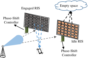
In a nutshell, the anatomy of the communication initiation is briefly explained as follows.

• •

  The BS broadcasts the UE identification number as a paging message.

• •

  Mobile receives the paging message and identifies itself along with its location to the BS and nearby RISs and a successful handshake between the BS and the UE takes place²² 2 It is noteworthy that angle of arrival of the UE’s response can be simply obtained by both the BS and RIS with passive localization methods [40]..

• •

  Subsequently, the BS which knows the location of the UE and fixed RISs around it, informs the UE and its nearest RIS which forward channel the UE has been assigned.

• •

  The associated RIS becomes an engaged RIS and its phase-controller adjusts the phase-shifts at the reflectors.

Assumption 2 : An engaged RIS is able to create a beam with highly narrow beamwidth toward the UE since it contains a large number of reflectors. Moreover, the reflection steering angle of each RIS is only limited to $[0,\quad\pi]$. Thus, it may receive signal only from a half of the interferer BSs³³ 3 Besides, since the RISs are passive and their reflected power significantly being affected by large-scale path-loss, they can only cause an interference for nearby UEs. . Intuitively, it significantly reduces the probability that the engaged RIS contributes to an effective interference. Therefore, throughout the paper, we neglect the interference that may be caused by engaged RIS reflections⁴⁴ 4 Recently, authors in [41] showed that the interference marginally increases by RISs deployments. However, in order to maximize the mathematical tractability, we ignore this limited interference..

In the following section, we explain the principles of the RIS-assisted mmWave cellular networks in more details.

Seeing that the RIS includes $M$ passive reflective elements, it does not generate any transmit power by its own. The phase controller of the RIS determines the phase-shift for each reflected signal to create a new beam towards the UE. Let assume that it is only able to adjust discrete phase-shifts for the impinging signal at each passive reflector due to the implementation constraints. In particular, in order to show the effect of $M$ passive reflectors of the RIS on the transmit power, and also the phase-shift at each reflector, let simplify the generic 2D phased-array by applying it into a 1D linear phased-array [42] as shown in Fig. 5; where the distance between the passive reflectors is denoted by $\ell$ and distance of the $m$th passive reflector to the UE is denoted by $d_{m}$, where $m=1,\cdots,M$. Let $s(t+\delta_{m})$ denote the message impinging the $m$th passive reflector at the RIS where $\delta_{m}$ stands for the phase difference of the impinging message at the $m$th reflector. Then, the reflected signal towards the UE which is a superposition due to $M$ passive reflectors is given by

where $c$, $\varphi$ and $\tau_{m}$ correspond to the wave-speed, angle of the $1$th element reflection toward the UE (as shown in Fig. 5) and time delay of the $m$th reflector. Here, the time delay, $\tau_{m}$, is associated with the phase-shift adjustment at the $m$th reflector. In other words, $\tau_{m}$ is given by

Therefore, the reflected signal in (11) becomes

Consequently, the RIS executes a new passive beamforming towards the UE, i.e., in an angle of $\varphi$, where the maximum power of the beam, i.e., peak effective radiated power, scales up by $M^{2}$. In addition, in order to put the phase-shift adjustment at each reflector into action, we may need to consider implementation constraints since $\frac{m\ell\cos\varphi}{c}+\delta_{m}$ might be continues values. However, we consider discrete values for $\tau_{m}$ that there will be a minimum phase-shift adjustment. We quantize the continues phase-shift amplitudes by discretizing them into the implementable values.

An important quantity is the distance between the engaged RIS and the associated BS, denoted by $r_{1}$, which affects the transmit power at the RIS considering the large-scale fading. Although the BSs and RISs are both distributed based on two independent homogeneous PPPs, i.e., $\Phi_{BS}$ and $\Phi_{RIS}$, $r_{1}$ depends on both $r_{0}$ and $r_{2}$ as shown in Fig. 6. Therefore, the distribution of $r_{1}$ for given $r_{0}$ and $r_{2}$ equals the captured annulus of the circumference of the circle with a radius of $r_{2}$ and origin of the UE as shown in Fig. 6. Hence, the CDF of $r_{1}$ becomes the probability of the engaged RIS located on annulus of $2\theta r_{2}$ over the whole possible area of the circumference of $2\pi r_{2}$ as follows:

From the law of Cosines in the shaded triangle⁵⁵ 5 $a^{2}=b^{2}+c^{2}-2bc\cos(\hat{A})$, we have

By substituting (15) in (14) we have

Then, the PDF of $r_{1}$ for given $r_{0}$ and $r_{2}$ can be obtained as

It is noteworthy that the $r_{1}$ can vary from $|r_{0}-r_{2}|$ to $r_{0}+r_{2}$. Eventually, from (1) and (7), the PDF of the $r_{1}$ is given by

Fig. 7 shows the theoretical PDF of the $r_{1}$ which coincides with the simulation results. In addition, in order to see the impact of $\lambda_{RIS}$ and $\lambda_{BS}$ on the $r_{1}$, the expected value of $r_{1}$ in (18) with putting its condition into the integral becomes

Thus, we have

This integral is numerically calculated using MATLAB as a function of $\mathcal{F}_{r_{1}}\left(\lambda_{RIS},\lambda_{BS}\right)\triangleq\mathbb{E}\{r_{1}\}$ which Fig. 8 shows its changes when $\lambda_{RIS}$ and $\lambda_{BS}$ vary. In general, an increase in either of $\lambda_{RIS}$ or $\lambda_{BS}$ reduces $\mathbb{E}\{r_{1}\}$. For example, for a fixed $\lambda_{BS}$, if $\lambda_{RIS_{a}}<\lambda_{RIS_{b}}$, then $\mathcal{F}_{r_{1}}\left(\lambda_{RIS_{a}},\lambda_{BS}\right)>\mathcal{F}_{r_{1}}\left(\lambda_{RIS_{b}},\lambda_{BS}\right)$. However, the speed of changes in $\mathcal{F}_{r_{1}}$ decreases when $\lambda_{RIS}$ increases. Therefore, we can conclude that from law of large numbers (LLN) theorem, if $\lambda_{RIS_{a}}<\lambda_{RIS_{b}}$, $\lambda_{BS_{a}}<\lambda_{BS_{b}}$ and $\lambda_{BS_{a}},\lambda_{BS_{b}},\lambda_{RIS_{a}},\lambda_{RIS_{b}}\rightarrow\infty$, then $\mathcal{F}_{r_{1}}\left(\lambda_{RIS_{a}},\lambda_{BS_{b}}\right)\approx\mathcal{F}_{r_{1}}\left(\lambda_{RIS_{b}},\lambda_{BS_{b}}\right)$ in large-scale communications.

The transmitted signal from the associated BS towards the engaged RIS experiences a small-scale fading gain, denoted by $f_{m}$, while reaching at the $m$th RIS-reflector, i.e., from Assumption 1, we assume $f_{m}\sim\exp(\mu)$. Thus, the impinging signal power at the $m$th passive RIS-reflector is given by

Since the RIS-reflectors are located in a relatively short distance from each other, we can assume $f_{m}$ is likely correlated and for a given $r_{1}$, we can conclude that

Let us assume an attenuation power factor for RIS-reflectors which is denoted by $\beta\in(0,\quad 1]$. Here, $\beta$ is constant and can be obtained by measuring the attenuation power of a signal passing through the RIS-reflectors. Furthermore, since the peak effective radiated power scales up by $M^{2}$ as given in (13), the peak reflected power from the engaged RIS towards the UE becomes

Consequently the reflected power largely affected by $r_{1}^{-\alpha}$. With respect to (19), the average peak reflected power can be expressed as a function of $\lambda_{RIS}$ and $\lambda_{BS}$ for given $\alpha,\,\beta$ and $M$ as follows

which is shown in Fig. 9. In other words, the dependency of average power on $\lambda_{RIS}$ and $\lambda_{BS}$ comes from $\tilde{\mathcal{F}}_{r_{1}}\left(\lambda_{RIS},\lambda_{BS}\right)\triangleq\mathbb{E}\{r_{1}^{-\alpha}\}$ with respect to the PDF of $r_{1}$ in (18) and (19). Thus, we conclude that in general, since $\alpha$ is positive, i.e., usually $\alpha>2$ [3], the average reflected power from the RIS increases when $\lambda_{RIS}$ increases, i.e., $\mathbb{E}\{r_{1}\}$ decreases. For example, keeping $\lambda_{BS}$ fixed, if $\lambda_{RIS_{a}}<\lambda_{RIS_{b}}$, then $\mathcal{F}_{P}\left(\lambda_{RIS_{a}},\lambda_{BS}\right)<\mathcal{F}_{P}\left(\lambda_{RIS_{b}},\lambda_{BS}\right)$. Likewise, the reflected power from the RIS decreases when BS density decreases as shown in Fig. 9. However, this reflected power reduction can be compensated by employing larger RISs with more number of reflectors, i.e., a larger $M$.

In order to find the SIR coverage probability of the RIS-assisted path, i.e., path B, and simplify the analysis in section IV, we introduce a raw moment of $\left(\frac{P_{\text{RIS}}}{\mu}\right)^{\frac{2}{\alpha}}$ which is calculated as follows:

Since $f_{1}\sim\exp(\mu)$, we have

where $\Gamma(x)=\int_{0}^{\infty}t^{x-1}e^{-}t\,dt$ is the Gamma function. Moreover, from (18), we define

where $\varepsilon=\max\left(|r_{0}-r_{2}|,\epsilon\right)$ and $\epsilon$ is a minimum euclidean distance of the BS from the RIS that prevents the divergence of $\mathbb{E}\left\{r_{1}^{-2}\right\}$. Eventually, by substituting (25) and (26) in (24), we have

Remark 1: The raw moment of $\left(\frac{P_{\text{RIS}}}{\mu}\right)^{\frac{2}{\alpha}}$ in (27) depends on $\mathcal{F}_{R}\left(\lambda_{RIS},\lambda_{BS}\right)$ for given $\alpha,\,M,\,\mu$ and $\beta$. Therefore, similar to the $\mathcal{F}_{P}\left(\lambda_{RIS},\lambda_{BS}\right)\triangleq\mathbb{E}\{P_{\text{RIS}}\}$ shown in Fig. 9, $\mathbb{E}\left\{\left(\frac{P_{\text{RIS}}}{\mu}\right)^{\frac{2}{\alpha}}\right\}$ is an increasing function of $\lambda_{RIS}$ and $\lambda_{BS}$.

In this approximation, from (1) and (7), we have

Therefore, we simply approximate

where $\rho=\sqrt{\frac{\tilde{\lambda}_{BS}}{\tilde{\lambda}_{RIS}}}$. Consequently we define the following proposition.

In this approximation we consider a lower bound where $\lambda_{RIS}\gg\lambda_{BS}\rightarrow\upsilon\geqslant r_{2}$ in (41). Therefore, we state the following proposition.

Since the selection diversity of the two received signals is taken into account in the proposed RIS-assisted model, the UE is able to select the strongest signal between those received signals through paths A and B. Fig. 10 compares the SIR coverage probabilities for both of paths A and B. Based on (30), (44) and (50), $\Gamma_{\textbf{A}}$ only depends on $N$ while $\Gamma_{\textbf{B}}$ depends on $\lambda_{RIS}$ as well. Therefore, it is shown that when $\lambda_{RIS}$ increases from $5\times 10^{-4}$ to $0.05$ $\frac{RIS}{m^{2}}$, $\Gamma_{\textbf{B}}$ is improved. Moreover, when $\lambda_{RIS}$ becomes larger, i.e., $\lambda_{RIS}\gg\lambda_{BS}$, $\Gamma_{\textbf{B}}$ outperforms $\Gamma_{\textbf{A}}$.

Fig. 11 compares the the coverage performance of the proposed model with the baseline model. It shows that there is a minimum coverage probability when there is no RIS-assisted path between the BS and the UE, i.e., small $\lambda_{RIS}$ results in $\Gamma_{\textbf{s}}=\Gamma_{\textbf{A}}$ which is independent of $\lambda_{RIS}$, e.g., $\lambda_{RIS}=10^{-5}$ $\frac{RIS}{m^{2}}$. This minimum coverage probability is slightly less than that of the baseline model since we have two beams in the RIS assisted model while there is only one beam in the baseline model with the same BS structure. In other words, with fixed $N$ active antennas at the BSs, the beam in the baseline model is narrower that that of the RIS-assisted model causes less co-channel interference. However, when $\lambda_{RIS}$ increases, the coverage probability in the RIS-assisted is improved. In addition, bigger RISs, i.e., a larger $M$, performs better than small RISs as it increases the reflected power from the engaged RIS.

Fig. 12 shows the impact of $\lambda_{RIS}$ on the proposed RIS-assisted model. As discussed in section V, when $\lambda_{RIS}$ increases, the SIR coverage probability of $\Gamma_{\textbf{B}}$ approaches 1. Moreover, we can see that Approximation I is supported by the simulation results in high $\lambda_{RIS}$ because when $\lambda_{RIS}\rightarrow\infty$, the distance of $r_{2}$ and its variations becomes smaller; therefore, $r_{2}\approx\rho r_{0}$ in (43) becomes more realistic. In addition, the SIR performances for the baseline model and the path A in the RIS-assisted model are fixed and independent from the $\lambda_{RIS}$ variations. $\Gamma_{\textbf{o}}$ has better performance compared to $\Gamma_{A}$ due to having a narrower beamwidth since it uses all $N$ elements to create one beam while in the proposed model there are two wider beams with the same BS structure.

Fig. 13 depicts the SIR coverage performance of the RIS-assisted and the baseline model with respect to $\lambda_{BS}$. As $\lambda_{BS}$ increases, $\Gamma_{\textbf{o}}$ and $\Gamma_{\textbf{A}}$ remain unchanged while $\Gamma_{\textbf{B}}$ slightly decreases. It shows that although higher $\lambda_{BS}$ leads to a higher reflected power from the RIS, its impact on the co-channel interference power is larger. In other words, the speed of increasing of co-channel interference power is faster than that of reflected power from the RIS.

References

- [1] GSM Association (GSMA), “White paper: Study on socio-economic benefits of 5G services provided in mmWave bands,” tech. rep., ROSCONGRESS, December-2018.
- [2] Ericsson Inc., “White paper: Ericsson Mobility Report June 2019,” tech. rep., Ericsson, June 2019.
- [3] S. Rangan, T. S. Rappaport, and E. Erkip, “Millimeter-Wave Cellular Wireless Networks: Potentials and Challenges,” Proceedings of the IEEE, vol. 102, no. 3, pp. 366–385, 2014.
- [4] J. Ding, M. Nemati, C. Ranaweera, and J. Choi, “IoT Connectivity Technologies and Applications: A Survey,” IEEE Access, vol. 8, pp. 67646–67673, 2020.
- [5] K. Ntontin and C. Verikoukis, “Relay-Aided Outdoor-to-Indoor Communication in Millimeter-Wave Cellular Networks,” IEEE Systems Journal, 2019.
- [6] T. Bai and R. W. Heath, “Coverage and Rate Analysis for Millimeter-Wave Cellular Networks,” IEEE Transactions on Wireless Communications, vol. 14, no. 2, pp. 1100–1114, 2015.
- [7] T. S. Rappaport, R. W. Heath Jr, R. C. Daniels, and J. N. Murdock, Millimeter wave wireless communications. Pearson Education, 2015.
- [8] T. S. Rappaport, Y. Xing, O. Kanhere, S. Ju, A. Madanayake, S. Mandal, A. Alkhateeb, and G. C. Trichopoulos, “Wireless Communications and Applications Above 100 GHz: Opportunities and Challenges for 6G and Beyond,” IEEE Access, vol. 7, pp. 78729–78757, 2019.
- [9] G. Yang and M. Xiao, “Performance Analysis of Millimeter-Wave Relaying: Impacts of Beamwidth and Self-Interference,” IEEE Transactions on Communications, vol. 66, no. 2, pp. 589–600, 2018.
- [10] K. Belbase, Analysis of Millimeter Wave Wireless Relay Networks. PhD thesis, 2019.
- [11] K. RISNTO, M. Renzo, J. Song, F. Lazarakis, J. Rosny, D.-T. Phan-Huy, O. Simeone, R. Zhang, M. Debbah, G. Lerosey, M. Fink, S. Tretyakov, and S. Shamai, “Reconfigurable Intelligent Surfaces vs. Relaying: Differences, Similarities, and Performance Comparison,” 08 2019.
- [12] E. Basar, M. Di Renzo, J. De Rosny, M. Debbah, M. Alouini, and R. Zhang, “Wireless Communications Through Reconfigurable Intelligent Surfaces,” IEEE Access, vol. 7, pp. 116753–116773, 2019.
- [13] Q. Wu and R. Zhang, “Towards Smart and Reconfigurable Environment: Intelligent Reflecting Surface Aided Wireless Network,” IEEE Communications Magazine, vol. 58, no. 1, pp. 106–112, 2020.
- [14] J. Park, S. Samarakoon, H. Shiri, M. K. Abdel-Aziz, T. Nishio, A. Elgabli, and M. Bennis, “Extreme URLLC: Vision, Challenges, and Key Enablers,” arXiv preprint arXiv:2001.09683, 2020.
- [15] M. Nemati, J. Ding, and J. Choi, “Short-range ambient backscatter communication using reconfigurable intelligent surfaces,” in 2020 IEEE Wireless Communications and Networking Conference (WCNC), pp. 1–6, 2020.
- [16] J. G. Andrews, T. Bai, M. N. Kulkarni, A. Alkhateeb, A. K. Gupta, and R. W. Heath, “Modeling and Analyzing Millimeter Wave Cellular Systems,” IEEE Transactions on Communications, vol. 65, no. 1, pp. 403–430, 2017.
- [17] S. Singh, F. Ziliotto, U. Madhow, E. Belding, and M. Rodwell, “Blockage and directivity in 60 GHz wireless personal area networks: from cross-layer model to multihop MAC design,” IEEE Journal on Selected Areas in Communications, vol. 27, no. 8, pp. 1400–1413, 2009.
- [18] S. Biswas, S. Vuppala, J. Xue, and T. Ratnarajah, “On the Performance of Relay Aided Millimeter Wave Networks,” IEEE Journal of Selected Topics in Signal Processing, vol. 10, no. 3, pp. 576–588, 2016.
- [19] S. Gong, X. Lu, D. T. Hoang, D. Niyato, L. Shu, D. I. Kim, and Y. Liang, “Towards smart wireless communications via intelligent reflecting surfaces: A contemporary survey,” IEEE Communications Surveys Tutorials, pp. 1–1, 2020.
- [20] I. Trigui, W. Ajib, and W.-P. Zhu, “A Comprehensive Study of Reconfigurable Intelligent Surfaces in Generalized Fading,” arXiv preprint arXiv:2004.02922, 2020.
- [21] Y. Liu, X. Liu, X. Mu, T. Hou, J. Xu, Z. Qin, M. Di Renzo, and N. Al-Dhahir, “Reconfigurable Intelligent Surfaces: Principles and Opportunities,” arXiv preprint arXiv:2007.03435, 2020.
- [22] Q. Wu, S. Zhang, B. Zheng, C. You, and R. Zhang, “Intelligent reflecting surface aided wireless communications: A tutorial,” arXiv preprint arXiv:2007.02759, 2020.
- [23] T. Hou, Y. Liu, Z. Song, X. Sun, Y. Chen, and L. Hanzo, “Reconfigurable intelligent surface aided noma networks,” IEEE Journal on Selected Areas in Communications, pp. 1–1, 2020.
- [24] X. Yue and Y. Liu, “Performance analysis of intelligent reflecting surface assisted NOMA networks,” arXiv preprint arXiv:2002.09907, 2020.
- [25] C. Zhang, W. Yi, Y. Liu, Z. Qin, and K. K. Chai, “Downlink analysis for reconfigurable intelligent surfaces aided noma networks,” arXiv preprint arXiv:2006.13260, 2020.
- [26] M. A. Kishk and M.-S. Alouini, “Exploiting randomly-located blockages for large-scale deployment of intelligent surfaces,” arXiv preprint arXiv:2001.10766, 2020.
- [27] T. Hou, Y. Liu, Z. Song, X. Sun, Y. Chen, and L. Hanzo, “MIMO assisted networks relying on large intelligent surfaces: A stochastic geometry model,” arXiv preprint arXiv:1910.00959, 2019.
- [28] M. Di Renzo and J. Song, “Reflection probability in wireless networks with metasurface-coated environmental objects: an approach based on random spatial processes,” EURASIP Journal on Wireless Communications and Networking, vol. 2019, no. 1, p. 99, 2019.
- [29] J. He, K. Yu, and Y. Shi, “Coordinated passive beamforming for distributed intelligent reflecting surfaces network,” arXiv preprint arXiv:2002.05915, 2020.
- [30] Q. Nadeem, A. Kammoun, A. Chaaban, M. Debbah, and M. Alouini, “Asymptotic Max-Min SINR Analysis of Reconfigurable Intelligent Surface Assisted MISO Systems,” IEEE Transactions on Wireless Communications, pp. 1–1, 2020.
- [31] J. G. Andrews, F. Baccelli, and R. K. Ganti, “A tractable approach to coverage and rate in cellular networks,” IEEE Transactions on communications, vol. 59, no. 11, pp. 3122–3134, 2011.
- [32] M. Rebato, J. Park, P. Popovski, E. De Carvalho, and M. Zorzi, “Stochastic Geometric Coverage Analysis in mmWave Cellular Networks With Realistic Channel and Antenna Radiation Models,” IEEE Transactions on Communications, vol. 67, no. 5, pp. 3736–3752, 2019.
- [33] D. Moltchanov, “Distance distributions in random networks,” Ad Hoc Networks, vol. 10, no. 6, pp. 1146 – 1166, 2012.
- [34] J. Park, S. Kim, and J. Zander, “Tractable Resource Management With Uplink Decoupled Millimeter-Wave Overlay in Ultra-Dense Cellular Networks,” IEEE Transactions on Wireless Communications, vol. 15, no. 6, pp. 4362–4379, 2016.
- [35] Y. Li, J. G. Andrews, F. Baccelli, T. D. Novlan, and C. J. Zhang, “Design and Analysis of Initial Access in Millimeter Wave Cellular Networks,” IEEE Transactions on Wireless Communications, vol. 16, no. 10, pp. 6409–6425, 2017.
- [36] J. Kim, J. Park, S. Kim, S. Kim, K. W. Sung, and K. S. Kim, “Millimeter-Wave Interference Avoidance via Building-Aware Associations,” IEEE Access, vol. 6, pp. 10618–10634, 2018.
- [37] Z. Limani, F. Malandrino, C. F. Chiasserini, and A. Nordio, “Mmwave beam management in urban vehicular networks,” arXiv preprint arXiv:2005.09726, 2020.
- [38] K. Venugopal, M. C. Valenti, and R. W. Heath, “Interference in finite-sized highly dense millimeter wave networks,” in 2015 Information Theory and Applications Workshop (ITA), pp. 175–180, 2015.
- [39] K. Belbase, Z. Zhang, H. Jiang, and C. Tellambura, “Coverage Analysis of Millimeter Wave Decode-and-Forward Networks With Best Relay Selection,” IEEE Access, vol. 6, pp. 22670–22683, 2018.
- [40] M. Nemati, T. Baykas, and J. Choi, “Performance of TDOA and AOA Localization Techniques for Different Base-Stations Topologies,” in 2019 13th International Conference on Signal Processing and Communication Systems (ICSPCS), pp. 1–7, 2019.
- [41] J. Lyu and R. Zhang, “Hybrid Active/Passive Wireless Network Aided by Intelligent Reflecting Surface: System Modeling and Performance Analysis,” arXiv preprint arXiv:2004.13318, 2020.
- [42] V. Giurgiutiu, “Chapter 6 - Piezoelectric Wafer Active Sensors,” in Structural Health Monitoring of Aerospace Composites (V. Giurgiutiu, ed.), pp. 177 – 248, Oxford: Academic Press, 2016.
- [43] X. Zhang and M. Haenggi, “The Performance of Successive Interference Cancellation in Random Wireless Networks,” IEEE Transactions on Information Theory, vol. 60, no. 10, pp. 6368–6388, 2014.
- [44] M. Haenggi and R. Ganti, “Interference in Large Wireless Networks,” Foundations and Trends in Networking, vol. 3, pp. 127–248, 01 2009.