On diagonal dominance of FEM stiffness matrix of fractional Laplacian and maximum principle preserving schemes for fractional Allen-Cahn equationThanks: ¹School of Mathematical Sciences, University of Electronic Science and Technology of China, Chengdu Sichuan 611731, China. Email: hyliu@std.uestc.edu.cn (H. Liu).
²Division of Mathematical Sciences, School of Physical and Mathematical Sciences, Nanyang Technological University, 637371, Singapore. The research of the authors is partially supported by Singapore MOE AcRF Tier 2 Grants: MOE2018-T2-1-059 and MOE2017-T2-2-144. Emails: ctsheng@ntu.edu.sg (C. Sheng) and lilian@ntu.edu.sg (L. Wang).
³Department of Mathematics, Southern University of Science and Technology, Shenzhen, 518055, China, and School of Mathematics and Statistics, Wuhan University, Wuhan, 430072, China. Email: yuanhf@sustech.edu.cn (H. Yuan).
The first and last two authors would like to thank NTU for hosting their visits devoted to this collaborative work.

Hongyan Liu¹, Changtao Sheng², Li-Lian Wang² and Huifang Yuan³

Abstract.

In this paper, we study diagonal dominance of the stiffness matrix resulted from the piecewise linear finite element discretisation of the integral fractional Laplacian under global homogeneous Dirichlet boundary condition in one spatial dimension. We first derive the exact form of this matrix in the frequency space which is extendable to multi-dimensional rectangular elements. Then we give the complete answer when the stiffness matrix can be strictly diagonally dominant. As one application, we apply this notion to the construction of maximum principle preserving schemes for the fractional-in-space Allen-Cahn equation, and provide ample numerical results to verify our findings.

Key words and phrases:

Diagonal dominance, Maximum principle, integral fractional Laplacian, fractional-in-space Allen-Cahn equation.

2000 Mathematics Subject Classification

35B50, 41A05, 41A25, 74S05.

1. Introduction

The study of diagonal dominance of a matrix has been a research subject of longstanding interest in numerical linear algebra and numerical analysis (cf. [18, 16]). On one hand, this type of structured matrices enjoy appealing properties, such as stable Gaussian elimination without pivoting and guaranteed convergence of Jacobi and Gauss-Seidel iterations among others (cf. [3, 15, 13]). On the other hand, numerical methods for solving PDEs are a rich source of many linear systems whose coefficient matrices form diagonal dominant matrices (cf. [36, 25, 35]). One well-worn example is the matrix resulted from the piecewise finite element discretization of $u^{\prime\prime}(x)$ with homogeneous Dirichlet boundary conditions on a uniform partition of a finite interval. However, this property is unknown to date for the fractional counterpart $(-\Delta)^{s}u(x)$ . The main purpose of this paper is to provide a complete answer to this and discuss one of its applications.

We consider a piecewise linear finite element approximation of the fractional Poisson equation on the finite interval $\Omega=(a,b)$ with $s\in(0,3/2)$ :

(-\Delta)^{s}u(x)=f(x),\;\;\;x\in\Omega;\quad u(x)=0,\;\;\;x\in\Omega^{c},

(1.1)

where the integral fractional Laplacian operator takes the form

(-\Delta)^{s}u(x)=C_{s}\,{\rm p.v.}\!\int_{\mathbb{R}}\frac{u(x)-u(y)}{|x-y|^{1+2s}}{\rm d}y,\quad C_{s}:=\frac{2^{2s}s\Gamma(s+1/2)}{\sqrt{\pi}\Gamma(1-s)},

(1.2)

or equivalently by the Fourier transform:

(-\Delta)^{s}u(x)={\mathscr{F}}^{-1}\big[|\xi|^{2s}\mathscr{F}{\left[u\right]}({\xi})\big](x).

(1.3)

Let $\{\phi_{j}\}_{j=1}^{N-1}$ be a set of $C^{0}$ -piecewise linear nodal basis associated with a uniform partition of $\Omega$ with mesh size $h$ . Different from the computation in the physical space based on (1.2) (cf. [37]), we evaluate the entries of the fractional stiffness matrix $\bm{S}$ in the frequency space using (1.3):

S_{kj}=S_{jk}=\big((-\Delta)^{s/2}\phi_{j},(-\Delta)^{s/2}\phi_{k}\big)_{\mathbb{R}}=\int_{\mathbb{R}}|\xi|^{2s}{\mathscr{F}}[\phi_{j}](\xi)\overline{{\mathscr{F}}[\phi_{k}](\xi)}\,{\rm d}\xi,

(1.4)

which leads to the explicit expression of this symmetric Toeplitz matrix (see Theorem 2.1). Remarkably, this approach can be extended to rectangular tensorial finite elements in two or three-dimensional rectangular or L-shaped domains by reducing $2d$ -dimensional integrals into one- or two-dimensional integrals using polar or spherical coordinates (which we shall report in a separate paper). It is important to remark that the computation of the stiffness matrix in two-dimensions on unstructured meshes is much involved (cf. [1, 2]). It is also noteworthy of the recent works on quadrature-based finite difference methods for integral fractional Laplacian on regular domains [34, 9, 11].

With the explicit form of $\bm{S}$ at our disposal, we can rigorously show that (see Theorem 2.2): (i) when the fractional order $s\in(s_{0},1]$ with $s_{0}\approx 0.2347,$ the stiffness matrix $\bm{S}$ is strictly diagonally dominant with positive diagonal entries; (ii) for $s\in(1,3/2),$ $\bm{S}$ is non-diagonally dominant, and each diagonal entry is strictly smaller than the summation of other entries (in magnitude) in the same row (except for the first and last rows); and (iii) for $s\in(0,s_{0}),$ there exists an $N_{0}(s)$ such that if $N<N_{0}(s),$ the strict diagonal dominance still holds. In fact, the smallest $N_{0}(s)$ is around $155$ attained at $s_{*}\approx 0.13$ and then increases rapidly as the distance $|s-s_{*}|$ (for $s\in(0,s_{0}))$ increases (see Table 2.1 and Figure 2.1 (b)).

The second purpose of this paper is to apply the notion of diagonal dominance to the construction of maximum principle preserving schemes for the fractional-in-space Allen-Cahn equation with spatial finite element discretisation. More precisely, we consider

\begin{cases}u_{t}+\epsilon^{2}(-\Delta)^{s}u+f(u)=0,\quad&x\in\Omega,\;\;t\in(0,T],\\ u(x,t)=0,\quad&x\in\Omega^{c}=\mathbb{R}\setminus\Omega,\;\;t\in[0,T],\\ u(x,0)=u_{0}(x),\quad&x\in\Omega,\end{cases}

(1.5)

where $f(u)=F^{\prime}(u)$ with

F(u)=\frac{u^{2}(u-1)^{2}}{4}\;\;\;{\rm so}\;\;\;f(u)=\frac{u(u-1)(2u-1)}{2}.

(1.6)

Different from the usual double-well potential with minima at $u=\pm 1$ , i.e., $F(u)=(u^{2}-1)^{2}/4$ , the modified $F(u)$ has minima at $u=0,1$ (cf. [21, 23, 10]), in view of the global “boundary condition” imposed on $\Omega^{c}$ . There has been much recent interest in numerical solutions of fractional-in-space models but with possibly different definitions of the fractional operator. For example, Burrage et al. [6] considered the solutions of fractional diffusion equations with the “discrete” fractional Laplacian obtained by first finding a matrix representation, $\bm{A}$ , of the Laplacian (by the finite element) and raising it to the same fractional power $\bm{A}^{s}$ . Bueno-Orovio et al. [5] considered the spectral fractional Laplacian and proposed Fourier spectral methods. In Hou et al. [19], Crank-Nicolson finite difference method for fractional-in-space Allen-Cahn equation with the fractional derivative:

\mathcal{L}^{\alpha}_{x}u(x):=\frac{1}{-2\cos(\frac{\pi\alpha}{2})}\big({}_{a}D_{x}^{\alpha}u+{}_{x}D_{b}^{\alpha}u\big)(x),\quad\alpha\in(1,2),

(1.7)

where ${}_{a}D_{x}^{\alpha}u$ and ${}_{x}D_{b}^{\alpha}$ denote the left and right Riemann-Liouville fractional derivatives defined on $\Omega$ , and the finite-difference matrix with the usual homogeneous boundary condition: $u|_{\partial\Omega}=0,$ was derived from [34]. The method in [19] can be directly extended to the multi-dimensional model with the directional fractional Laplacian $\mathcal{L}^{\alpha}_{x}u(x)=(\mathcal{L}^{\alpha}_{x_{1}}+\mathcal{L}^{\alpha}_{x_{2}}+\mathcal{L}^{\alpha}_{x_{3}})u(x)$ on $\Omega^{3}$ with $u(x)|_{\partial\Omega^{3}}=0,$ in light of the tensorial nature of the operator and domain. It is known that $\mathcal{L}^{\alpha}_{x}u(x)=(-\Delta)^{\alpha/2}u(x)$ on $\Omega$ , when $u=0$ on $\Omega^{c}$ and $\alpha\in(0,2)$ but $\alpha\not=1$ . However, under the local boundary condition: $u|_{\partial\Omega}=0,$ they are different. Recently, Duo and Wang [10] proposed quadrature-based finite difference method for (1.5) with the difference matrix obtained earlier in [11], where the approximation error $(-\Delta)^{s}u-(-\Delta)_{h}^{s}u$ is of order $h^{2}$ in $L^{\infty}$ -sense. Wang et al. [37] studied the finite element methods for the fractional-in-space Cahn-Hilliard equation. It is also noteworthy that there is a growing interest in time-fractional Allen-Cahn model (cf. [8, 23, 33, 39, 22]). Needless to say, the development of efficient numerical methods for the integer order Allen-Cahn/Cahn-Hilliard equations and more general phase-field models is continuously attracting much research attention. One can refer to the review paper [27] and the book chapter [7] for the state-of-the-art and comprehensive lists of references.

Different from the very limited existing works, we consider finite element discretisation in space with a modification similar to that in Xu et al. [38], and propose the semi-implicit and Crank-Nicolson schemes as advocated in [32, 31] for the integer-order Allen-Cahn equation. We show that the proposed schemes preserve maximum principle and energy dissipation (for $s\in(s_{0},1)$ ) at the discrete level. Though we focus on one dimensional in space, the methods can be extended to multiple dimensions with the directional fractional Laplacian $\mathcal{L}^{\alpha}_{x}u(x)$ and global homogeneous Dirichlet boundary condition. However, the construction of this type of schemes for the integral fractional Laplacian in multiple dimensions is still open, though such properties can be shown at the continuous level.

The rest of this paper is organised as follows. In Section 2, we present the exact form of the FEM stiffness matrix based on the Fourier definition with implementation in the Fourier space. More importantly, we prove the main result on the diagonal dominance of this matrix. In Section 3, we propose the semi-implicit and modified FEM schemes for the fractional-in-space Allen-Cahn equation, and show that they preserve the maximum principle and energy dissipation. In Section 4, we provide ample numerical results to support the theoretical results. The final section is for some concluding remarks.

2. Finite element method for fractional Laplacian

In this section, we derive the explicit stiffness matrix of the $C^{0}$ -piecewise linear FEM for the fractional Laplacian using the frequency domain. More importantly, we will study the diagonally dominant properties of the stiffness matrix for piecewise linear FEM.

2.1. Finite element method

Consider a uniform partition of the interval $\Omega=(a,b)$ :

x_{j}=a+jh,\quad 0\leq j\leq N,\quad h=2/N.

The piecewise linear FEM basis is given by

\phi_{j}(x)=\begin{cases}\frac{x-x_{j-1}}{h},\quad&{\rm if}\;\;x\in(x_{j-1},x_{j}),\\[2.0pt] \frac{x_{j+1}-x}{h},\quad&{\rm if}\;\;x\in(x_{j},x_{j+1}),\\[2.0pt] 0,\quad&\text{elsewhere on}\;\;\mathbb{R}.\end{cases}

(2.1)

Correspondingly, we define the piecewise linear finite element space

{\mathbb{V}}_{\!h}={\rm span}\{\phi_{j}(x),\;1\leq j\leq N-1\}.

(2.2)

and intend to evaluate the $(N-1)\times(N-1)$ fractional stiffness matrix $\bm{S}$ with the entries


$\displaystyle S_{kj}$	$\displaystyle=S_{jk}=\frac{C_{s}}{2}\int_{\Omega}\int_{\Omega}\frac{(\phi_{j}(x)-\phi_{j}(y))(\phi_{k}(x)-\phi_{k}(y))}{\|x-y\|^{d+2s}}\,{\rm d}x{\rm d}y$
	$\displaystyle\quad+C_{d,s}\int_{\Omega}\bigg(\int_{\Omega^{c}}\frac{1}{\|x-y\|^{d+2s}}{\rm d}y\bigg)\phi_{j}(x)\phi_{k}(x)\,{\rm d}x$	(2.3a)
	$\displaystyle=\int_{\mathbb{R}}\|\xi\|^{2s}{\mathscr{F}}[\phi_{j}](\xi)\overline{{\mathscr{F}}[\phi_{k}](\xi)}\,{\rm d}\xi,$	(2.3b)

for $1\leq k,j\leq N-1.$ The representation (2.3a) corresponds to the implementation in the physical space, while the formula (2.3b) is implemented in the frequency space.

The following formula on the Fourier transform of the FEM basis plays an important role in the evaluation of $\bm{S}$ .

Lemma 2.1.

Let $\{\phi_{j}\}$ be the FEM basis given in (2.1). Then we have

{\mathscr{F}}[\phi_{j}](\xi)=\frac{2h}{\sqrt{2\pi}}\frac{1-\cos(h\xi)}{(h\xi)^{2}}{e^{-{\rm i}x_{j}\xi}},\quad\forall\,\xi\in{\mathbb{R}},\;\;1\leq j\leq N-1.

(2.4)

Proof.

Using (2.1) and integration by parts, we obtain from direct calculation that

	$\displaystyle{\mathscr{F}}[\phi_{j}](\xi)=\frac{1}{\sqrt{2\pi}}\int_{\mathbb{R}}\phi_{j}(x)e^{-{\rm i}\xi x}{\rm d}x=\frac{1}{\sqrt{2\pi}}\int^{x_{j+1}}_{x_{j-1}}\phi_{j}(x)e^{-{\rm i}\xi x}{\rm d}x$
	$\displaystyle\quad=\frac{1}{h\sqrt{2\pi}}\Big\{\int^{x_{j}}_{x_{j-1}}(x-x_{j-1})e^{-{\rm i}\xi x}{\rm d}x+\int^{x_{j+1}}_{x_{j}}(x_{j+1}-x)e^{-{\rm i}\xi x}{\rm d}x\Big\}$
	$\displaystyle\quad=\frac{1}{h\sqrt{2\pi}}\Big\{\frac{-h}{{\rm i}\xi}e^{-{\rm i}x_{j}\xi}+\frac{1}{\xi^{2}}(e^{-{\rm i}x_{j}\xi}-e^{-{\rm i}x_{j-1}\xi})\Big\}$
	$\displaystyle\qquad+\frac{1}{h\sqrt{2\pi}}\Big\{\frac{h}{{\rm i}\xi}e^{-{\rm i}x_{j}\xi}-\frac{1}{\xi^{2}}(e^{-{\rm i}x_{j+1}\xi}-e^{-{\rm i}x_{j}\xi})\Big\}$
	$\displaystyle\quad=\frac{-1}{h\sqrt{2\pi}}\Big\{\frac{e^{-{\rm i}x_{j-1}\xi}-2e^{-{\rm i}x_{j}\xi}+e^{-{\rm i}x_{j+1}\xi}}{\xi^{2}}\Big\}$
	$\displaystyle\quad=\frac{-e^{-{\rm i}x_{j}\xi}}{h\sqrt{2\pi}}\Big\{\frac{e^{-{\rm i}h\xi}+e^{{\rm i}h\xi}-2}{\xi^{2}}\Big\}=\frac{2e^{-{\rm i}x_{j}\xi}}{h\sqrt{2\pi}}\Big\{\frac{1-\cos(h\xi)}{\xi^{2}}\Big\}.$

This ends the proof. ∎

With the aid of Lemma 2.1, we can obtain the entires of stiffness matrix $\bm{S}$ explicitly. Here, we sketch the derivation in Appendix A to avoid distraction from the main result.

Theorem 2.1.

For $s\in(0,\frac{3}{2})$ , the FEM stiffness matrix $\bm{S}=(\bm{S}_{kj})$ is a symmetric Toeplitz matrix given by

\bm{S}=\frac{h^{1-2s}}{2\Gamma(4-2s)\cos(s\pi)}\begin{bmatrix}t_{0}&\hskip-4.0ptt_{1}&t_{2}&\cdots&t_{N-4}&t_{N-3}&t_{N-2}\\[1.0pt] t_{1}&\hskip-4.0ptt_{0}&t_{1}&\hskip-4.0pt\ddots&\cdots&t_{N-4}&t_{N-3}\\[-1.0pt] t_{2}&\hskip-4.0ptt_{1}&t_{0}&\ddots&\hskip-4.0pt\ddots&\vdots&t_{N-4}\\[0.0pt] \vdots&\hskip-4.0pt\ddots&\hskip-4.0pt\ddots&\ddots&\hskip-4.0pt\ddots&\hskip-4.0pt\ddots&\vdots\\[2.0pt] t_{N-4}&\vdots&\hskip-4.0pt\ddots&\hskip-4.0pt\ddots&\hskip 8.0ptt_{0}&t_{1}&t_{2}\\[-2.0pt] t_{N-3}&t_{N-4}&\cdots&\hskip-4.0pt\ddots&\hskip 8.0ptt_{1}&t_{0}&t_{1}\\[3.0pt] t_{N-2}&t_{N-3}&t_{N-4}&\cdots&\hskip 8.0ptt_{2}&t_{1}&t_{0}\end{bmatrix},

(2.5)

which is generated by the vector $(t_{0},t_{1},\cdots,t_{N-2})$ in the first row or column of $\bm{S}$ with

\begin{split}t_{p}=\sum_{i=-2}^{2}c_{i}|p+i|^{3-2s},\quad c_{0}=6,\;\;c_{\pm 1}=-4,\;\;c_{\pm 2}=1.\end{split}

(2.6)

In particular, if $s=1/2$ , the entries of $\bm{S}$ should be obtained by

S_{kj}=\frac{1}{4}\lim_{s\to\frac{1}{2}}\frac{t_{p}}{\cos(s\pi)}=\frac{1}{2\pi}\sum_{i=-2}^{2}c_{i}(p+i)^{2}\ln|p+i|,\;\;\;\;p=|k-j|,

(2.7)

where we should understand that $(p+i)^{2}\ln|p+i|=0$ when $p+i=0.$

Remark 2.1.

Letting $s\to 0$ and $s\to 1$ , the matrix $\bm{S}$ in Theorem 2.1 reduces to the usual FEM mass matrix $\bm{M}$ and stiffness matrix $\bm{S}$ :

M_{kj}=h\begin{cases}{2/3,}&{j=k},\\ {1/6,}&{j=k\pm 1},\\ {0,}&{\text{otherwise}},\end{cases}\qquad S_{kj}=\frac{1}{h}\begin{cases}{2,}\;\;&{j=k},\\ {-1,}&{j=k\pm 1},\\ {0,}&{\text{otherwise,}}\end{cases}

respectively. ∎

Remark 2.2.

We point out that in 1D, it is feasible to compute $S_{jk}$ in the physical space using (2.3a) (cf. [34, 37]). However, the implementation in the physical space becomes very complicated (cf. [1, 2]). In fact, the frequency domain approach can be extended to multiple dimensional uniform rectangular elements, which leads to computing a one-dimensional integral on $(0,\pi/2)$ rather than $2\times 2$ -dimensional integrals in two dimensions. We shall report this in a separate work. ∎

2.2. Diagonal dominance of the stiffness matrix

We first make necessary preparations through the following two lemmas.

Lemma 2.2.

Let $s\in(0,\frac{3}{2})$ and $s\not=\frac{1}{2}.$

(i)

The element

t_{1}=t_{1}(s)=7+3^{3-2s}-2^{5-2s}

(2.8)

has a unique root $s_{0}\approx 0.2347$ in the interval $(0,\frac{1}{2}).$ Moreover, we have

\begin{cases}t_{1}>0,\;\;&{\rm if}\;\;s\in(0,s_{0})\cup(\frac{1}{2},\frac{3}{2}),\\ t_{1}<0,\;\;&{\rm if}\;\;s\in(s_{0},\frac{1}{2}).\end{cases}

(2.9)

(ii)

For $p\geq 2$ , we have

\begin{cases}t_{p}<t_{p+1}<0,\;\;\;\;&{\rm if}\;\;s\in(0,\frac{1}{2})\cup(1,\frac{3}{2}),\\ t_{p}>t_{p+1}>0,\;\;\;\;&{\rm if}\;\;s\in(\frac{1}{2},1),\\ t_{p}=0,\;\;&{\rm if}\;\;s=1.\end{cases}

(2.10)

Proof.

(i) By direct calculation, we find $t_{1}^{\prime}(s)=8(\ln 2)\,2^{3-2s}-2(\ln 3)\,3^{3-2s},$ which has a unique root

s^{\ast}=\frac{3}{2}-\frac{\ln(8\ln 2)-\ln(2\ln 3)}{2(\ln 3-\ln 2)}\approx 0.3584.

(2.11)

Moreover, $t_{1}(s)$ is descending in $(0,s^{*}),$ but asending in $(s^{*},\frac{3}{2})$ . As $t_{1}(0)=2$ and $t_{1}(s^{*})\approx-0.1856,$ $t_{1}(s)$ has a unique root in $(0,s^{*}).$ Using a root-finding method (e.g., the bisection method), we can easily find $s_{0}\approx 0.2347.$ Note that $s=\frac{1}{2}$ is the other unique root of $t_{1}(s)$ in the interval $(s^{*},\frac{3}{2}).$ Then we have the property (2.9) (cf. Figure 2.1(a)).

(ii) We next consider $p\geq 2$ . Denote $\alpha=3-2s$ , and rewrite $t_{p}$ in (2.6) as

\begin{split}t_{p}&=p^{\alpha}\Big\{6-4\Big\{\Big(1+\frac{1}{p}\Big)^{\alpha}+\Big(1-\frac{1}{p}\Big)^{\alpha}\Big\}+\Big\{\Big(1+\frac{2}{p}\Big)^{\alpha}+\Big(1-\frac{2}{p}\Big)^{\alpha}\Big\}\Big\}=\sum_{n=2}^{\infty}\frac{c_{n}^{(\alpha)}}{p^{2n-\alpha}},\end{split}

(2.12)

where we used the Taylor expansion of $(1+x)^{\alpha}$ , and

c_{n}^{(\alpha)}:=(2^{2n+1}-2^{3})\frac{\alpha(\alpha-1)\cdots(\alpha-2n+1)}{(2n)!}.

As $\alpha=3-2s\in(0,3)$ and $\alpha\neq 2$ , we have

\text{sign}(c_{n}^{(\alpha)})=-\text{sign}((\alpha-1)(\alpha-2))=-\text{sign}((2s-1)(s-1)).

Note that $t_{p}$ has the same sign as $c_{n}^{(\alpha)}.$ Thus, if $s\in(0,1/2)\cup(1,3/2)$ , then $c_{n}^{(\alpha)}<0,$ so $t_{p}<0$ and

\frac{c_{n}^{(\alpha)}}{p^{2n-\alpha}}<\frac{c_{n}^{(\alpha)}}{{(p+1)}^{2n-\alpha}},\;\;\;{\rm so}\;\;\;t_{p}<t_{p+1}.

On the other hand, if $s\in(\frac{1}{2},1)$ , then $c_{n}^{(\alpha)}>0,$ so $t_{p}<0,$ and

\frac{c_{n}^{(\alpha)}}{p^{2n-\alpha}}>\frac{c_{n}^{(\alpha)}}{{(p+1)}^{2n-\alpha}},\;\;\;{\rm so}\;\;\;t_{p}>t_{p+1}.

By (A.15), we have $t_{p}=0$ for $s=1$ and $p\geq 2.$ Thus, the property (2.10) holds. ∎

Refer to caption — (a) Graph of $t_{1}(s)$

Lemma 2.3.

For $s=\frac{1}{2}$ , we denote

r_{p}:=S_{kj}=\frac{1}{2\pi}\sum_{i=-2}^{2}c_{i}(p+i)^{2}\ln|p+i|,\quad 0\leq p=|k-j|\leq N-2.

(2.13)

Then we have

r_{0}>0;\quad r_{p}<r_{p+1}<0,\quad 1\leq p\leq N-3.

(2.14)

Proof.

Direct calculation from (2.13) leads to

\begin{split}&r_{0}=\frac{4}{\pi}\ln 2,\quad r_{1}=\frac{1}{2\pi}\big(9\ln 3-16\ln 2\big),\quad r_{2}=\frac{2}{\pi}\big(14\ln 2-9\ln 3\big),\\ &r_{3}=\frac{1}{\pi}\Big(27\ln 3-72\ln 2+\frac{25}{2}\ln 5\Big),\end{split}

and one verifies readily that $r_{1}<r_{2}<r_{3}<0.$

For $p\geq 3$ , we can rewrite $r_{p}$ as

\begin{split}r_{p}&=\frac{p^{2}}{2\pi}\bigg\{\Big(1-\frac{2}{p}\Big)^{2}\ln\Big(1-\frac{2}{p}\Big)+\Big(1+\frac{2}{p}\Big)^{2}\ln\Big(1+\frac{2}{p}\Big)\\ &\quad-4\Big(1-\frac{1}{p}\Big)^{2}\ln\Big(1-\frac{1}{p}\Big)-4\Big(1+\frac{1}{p}\Big)^{2}\ln\Big(1+\frac{1}{p}\Big)\bigg\}\\ &=\sum_{n=2}^{\infty}\frac{c_{n}}{p^{2n-2}},\quad\text{with}\ \ \ c_{n}=\frac{2-2^{2n-1}}{\pi n(2n-1)(n-1)},\end{split}

(2.15)

using the Taylor expansion

(1+x)^{2}\ln(1+x)=x+\frac{3}{2}x^{2}+2\sum_{n=1}^{\infty}\frac{(-1)^{n+1}x^{n+2}}{n(n+1)(n+2)}.

(2.16)

Since $c_{n}<0$ for $n\geq 2$ , we have $r_{p}<0$ , and

\frac{c_{n}}{p^{2n-2}}<\frac{c_{n}}{{(p+1)}^{2n-2}},\;\;\;{\rm so}\;\;\;r_{p}<r_{p+1}.

This completes the proof. ∎

With the above preparations, we are now ready to present the main result.

Theorem 2.2.

Let $s_{0}\approx 0.2347$ be the root of $t_{1}(s)=7+3^{3-2s}-2^{5-2s}$ as in Lemma 2.2, and denote

A_{s}:=\frac{1}{2\Gamma(4-2s)\cos(s\pi)}.

(2.17)

Then the stiffness matrix $\bm{S}=(S_{kj})$ stated in Theorem 2.1 has the following properties.

(i)

If $s\in[s_{0},1)$ , we have

$S_{kk}>0;\quad S_{kj}<0,\quad k\not=j,$ (2.18)

except for $S_{k,k\pm 1}=0$ for $s=s_{0},$ and the matrix $\bm{S}$ is strictly positive diagonally dominated, i.e.,

$S_{kk}>\sum_{k\not=j=1}^{N-1}|S_{kj}|,\quad 1\leq k\leq N-1.$ (2.19)
(ii)

If $s\in(0,s_{0})$ , we have $S_{kk},S_{k,k\pm 1}>0,S_{kj}<0$ for $|k-j|\geq 2,$ and

$S_{kk}-\sum_{k\not=j=1}^{N-1}|S_{kj}|>-\frac{4A_{s}t_{1}(s)}{h^{2s-1}},\quad 1\leq k\leq N-1,$ (2.20)

where $t_{1}\in(0,2)$ . However, the property (2.19) holds only for $N\leq N_{0}$ with

$N_{0}=\Big[2\Big(\frac{\gamma(s)}{t_{1}(s)}\Big)^{\frac{1}{2s}}\Big],\quad\gamma(s):=(1-2s)(1-s)(3-2s).$ (2.21)
(iii)

If $s\in(1,3/2)$ , we have $S_{kk}>0,S_{k,k\pm 1}<0,S_{kj}>0$ for $|k-j|\geq 2.$ The property (2.19) holds only for $k=1$ and $k=N-1,$ but in the contrary, we have that for $N\geq 4,$

$S_{kk}<\sum_{k\not=j=1}^{N-1}|S_{kj}|,\quad 2\leq k\leq N-2.$ (2.22)

Proof.

We only prove the results with even $N$ , since it is straightforward to prove the statements with odd $N$ . Before we consider different cases of $s,$ we first derive some common properties.

From the matrix form of $\bm{S}$ in (2.5), we find readily that for $1\leq k\leq N-1,$

\begin{split}&d_{k}:=|S_{kk}|-\sum_{k\not=j=1}^{N-1}|S_{kj}|=\frac{|A_{s}|}{h^{2s-1}}\Big(|t_{0}|-\sum_{p=1}^{k-1}|t_{p}|-\sum_{p=1}^{N-1-k}|t_{p}|\Big),\end{split}

(2.23)

and for $1\leq k\leq N-2,$

\begin{split}&d_{k+1}=d_{k}+\frac{|A_{s}|}{h^{2s-1}}\big(|t_{N-1-k}|-|t_{k}|\big).\end{split}

(2.24)

It is also evident that

d_{k}=d_{N-k},\quad 1\leq k\leq N-1,

(2.25)

so it suffices to study $d_{k}$ with $1\leq k\leq N/2.$ Moreover, using the property (2.10), we can derive from (2.24) that for $s\in(0,\frac{3}{2})$ and $s\not=\frac{1}{2},1,$

d_{2}>d_{3}>\cdots>d_{N/2}.

(2.26)

In the proof, we shall check the signs of $d_{1}$ and $d_{N/2}$ in most of the cases. For this purpose, we define

f_{q}:=q^{3-2s},\quad{\mathcal{G}}_{q}:=f_{q-1}-3f_{q}+3f_{q+1}-f_{q+2}.

(2.27)

Using (2.10) again, we find from direct calculation that for $s\in(\frac{1}{2},1),$

\begin{split}{\mathcal{S}}_{m}&:=\sum_{p=2}^{m}|t_{p}|=\sum_{p=2}^{m}t_{p}=\sum_{p=2}^{m}(f_{p-2}-4f_{p-1}+6f_{p}-4f_{p+1}+f_{p+2})\\ &=\sum_{q=0}^{3}f_{q}-4\sum_{q=1}^{3}f_{q}+6\sum_{q=2}^{3}f_{q}-4f_{3}-4f_{m-1}\\ &\quad+6\sum_{q=m-1}^{m}f_{q}-4\sum_{q=m-1}^{m+1}f_{q}+\sum_{q=m-1}^{m+2}f_{q}\\[4.0pt] &=-3f_{1}+3f_{2}-f_{3}-f_{m-1}+3f_{m}-3f_{m+1}+f_{m+2}={\mathcal{G}}_{1}-{\mathcal{G}}_{m},\end{split}

(2.28)

and for $s\in(0,\frac{1}{2})\cup(1,\frac{3}{2}),$

\begin{split}{\mathcal{S}}_{m}&:=\sum_{p=2}^{m}|t_{p}|=-\sum_{p=2}^{m}t_{p}={\mathcal{G}}_{m}-{\mathcal{G}}_{1}.\end{split}

(2.29)

From (2.23) and the above, we have

\begin{split}&d_{1}=\frac{|A_{s}|}{h^{2s-1}}\bigg(|t_{0}|-|t_{1}|-\sum_{p=2}^{N-2}|t_{p}|\bigg)=\frac{|A_{s}|}{h^{2s-1}}\left(|t_{0}|-|t_{1}|-{\mathcal{S}}_{N-2}\right),\\ &d_{N/2}=\frac{|A_{s}|}{h^{2s-1}}\bigg(|t_{0}|-2|t_{1}|-2\sum_{p=2}^{N/2-1}|t_{p}|\bigg)=\frac{|A_{s}|}{h^{2s-1}}\left(|t_{0}|-2|t_{1}|-2{\mathcal{S}}_{N/2-1}\right).\end{split}

(2.30)

Note that by (2.6), we have

t_{0}=2^{4-2s}-8=-8f_{1}+2f_{2},\quad t_{1}=7+3^{3-2s}-2^{5-2s}=7f_{1}-4f_{2}+f_{3}.

(2.31)

It is seen from (2.30) that the sign of $\mathcal{G}_{q}$ is important to determine the signs of $d_{1},d_{N/2}$ , so we rewrite it by using the Taylor expansion:

\begin{split}\mathcal{G}_{q}={(q+1)}^{\alpha}\Big\{\Big(1-\frac{2}{q+1}\Big)^{\alpha}-3\Big(1-\frac{1}{q+1}\Big)^{\alpha}-\Big(1+\frac{1}{q+1}\Big)^{\alpha}+3\Big\}=\sum_{n=3}^{\infty}\frac{\hat{c}_{n}^{(\alpha)}}{(q+1)^{n-\alpha}},\end{split}

(2.32)

where $\alpha=3-2s$ as before, and

\hat{c}_{n}^{(\alpha)}:=(-1)^{n}(2^{n}-(-1)^{n}-3)\frac{\alpha(\alpha-1)\cdots(\alpha-n+1)}{n!}.

(2.33)

Since $\alpha\in(0,3),$ we have

\text{sign}(\mathcal{G}_{q})=\text{sign}(\hat{c}_{n}^{(\alpha)})=-\text{sign}((\alpha-1)(\alpha-2))=-\text{sign}((2s-1)(s-1)).

(2.34)

With these, we now proceed with the proof by considering several cases with different ranges of $s$ .

(i)₁. $s\in(\frac{1}{2},1)$ : In order to prove Statement-(i), we first consider $s\in(\frac{1}{2},1).$ Note that $A_{s}<0$ (cf. (2.17)), $t_{0}=2^{4-2s}-8<0$ and $t_{p}>0$ with $p\geq 1$ (cf. Lemma 2.2), so we have

S_{kk}=\frac{A_{s}t_{0}}{h^{2s-1}}>0;\quad S_{kj}=\frac{A_{s}t_{p}}{h^{2s-1}}<0,\;\;\;{\rm for}\;\;p=|k-j|\geq 1.

(2.35)

In view of (2.26), we only need to show that $d_{1}>0$ and $d_{N/2}>0.$ By (2.27)-(2.28) and (2.30)-(2.31),

\begin{split}&d_{1}=\frac{A_{s}}{h^{2s-1}}\big(t_{0}+t_{1}+\mathcal{S}_{N-2}\big)=\frac{A_{s}}{h^{2s-1}}\big(\frac{1}{2}t_{0}-{\mathcal{G}}_{N-2}\big),\end{split}

(2.36)

and

\begin{split}d_{N/2}&=\frac{A_{s}}{h^{2s-1}}\big(t_{0}+2t_{1}+2\mathcal{S}_{N/2-1}\big)=-\frac{2A_{s}}{h^{2s-1}}\mathcal{G}_{N/2-1}.\end{split}

(2.37)

For $s\in(1/2,1),$ we know from (2.34) that ${\mathcal{G}}_{N-2},\mathcal{G}_{N/2-1}>0.$ As $A_{s}<0,$ we infer from (2.36)-(2.37) that $d_{1},d_{N/2}>0,$ so the desired property (2.19) holds for $s\in(1/2,1).$

(i)₂. $s\in[s_{0},\frac{1}{2})$ : In this case, we have $A_{s}>0$ (cf. (2.17)), $t_{0}=2^{4-2s}-8>0$ , and $t_{p}<0$ for $p\geq 1$ (except for $t_{1}=0$ with $s=s_{0},$ see Lemma 2.2), so their signs are opposite to those of the previous case. As a result, the property (2.18) still holds, but with the exceptional case: $S_{k,k\pm 1}=0,$ if $s=s_{0}.$ Moreover, we also have the same formulas as (2.36)-(2.37) for $d_{1},d_{N/2}$ , i.e.,

d_{1}=\frac{A_{s}}{h^{2s-1}}\Big(\frac{1}{2}t_{0}-{\mathcal{G}}_{N-2}\Big),\quad d_{N/2}=-\frac{2A_{s}}{h^{2s-1}}\mathcal{G}_{N/2-1},

but by (2.34), we have ${\mathcal{G}}_{N-2},\mathcal{G}_{N/2-1}<0,$ so $d_{1},d_{N/2}>0.$ Consequently, Statement-(i) holds for $s\in[s_{0},1/2).$

(i) ${}_{3}.$ $s=\frac{1}{2}$ : It is evident that by Lemma 2.3, we have $S_{kk}>0$ and $S_{kj}<0$ for $k\not=j.$ Moreover, $d_{k}$ in (2.23) becomes

\begin{split}&d_{k}:=|S_{kk}|-\sum_{k\not=j=1}^{N-1}|S_{kj}|=r_{0}+\sum_{p=1}^{k-1}r_{p}+\sum_{p=1}^{N-1-k}r_{p}.\end{split}

Similarly, we have $d_{k}=d_{N-k},$ and

d_{k+1}=d_{k}+r_{k}-r_{N-1-k}<d_{k},\quad 1\leq k\leq N/2-1.

In this case, it is only necessary to show that $d_{N/2}>0.$ Comparing (2.13) with (2.6), the formulas in (2.27)-(2.28) are valid in place of $f_{q}=\frac{1}{2\pi}q^{2}\ln q$ and $t_{p}=r_{p}$ in $\mathcal{G}_{q}.$ Like (2.37), we have

\begin{split}d_{N/2}&=-{\mathcal{G}}_{N/2-1}=\frac{1}{\pi}\bigg\{\Big(\frac{N}{2}+1\Big)^{2}\ln\Big(\frac{N}{2}+1\Big)-3\Big(\frac{N}{2}\Big)^{2}\ln\frac{N}{2}\\ &\qquad+3\Big(\frac{N}{2}-1\Big)^{2}\ln\Big(\frac{N}{2}-1\Big)-\Big(\frac{N}{2}-2\Big)^{2}\ln\Big(\frac{N}{2}-2\Big)\bigg\}\\ &=\frac{N^{2}}{4\pi}\bigg\{\Big(1+\frac{2}{N}\Big)^{2}\ln\Big(1+\frac{2}{N}\Big)+3\Big(1-\frac{2}{N}\Big)^{2}\ln\Big(1-\frac{2}{N}\Big)-\Big(1-\frac{4}{N}\Big)^{2}\ln\Big(1-\frac{4}{N}\Big)\bigg\},\end{split}

where we subtracted a summation of five terms with $\ln\frac{N}{2}$ in place of all five $\ln$ s (which is zero). Using the Taylor expansion (2.16), we can expand $d_{N/2}$ as

d_{N/2}=\frac{2}{\pi}\sum_{n=1}^{\infty}\frac{2^{n+2}+(-1)^{n+1}-3}{n(n+1)(n+2)}\Big(\frac{2}{N}\Big)^{n},

(2.38)

which is apparently positive. Thus, Statement-(i) is valid for $s=\frac{1}{2}.$

(ii). $s\in(0,s_{0})$ : We now turn to the justification for Statement-(ii). In this case, we have $A_{s}>0,t_{0}>0,t_{1}>0$ and $t_{p}<0$ for $p\geq 2.$ We first show that $d_{1}>0.$ Indeed, by (2.27) and (2.29)-(2.31),

\begin{split}d_{1}&=\frac{A_{s}}{h^{2s-1}}\bigg(t_{0}-t_{1}-\sum_{p=2}^{N-2}|t_{p}|\bigg)=\frac{A_{s}}{h^{2s-1}}\big(9\cdot 2^{\alpha}-2\cdot{3}^{\alpha}-18-\mathcal{G}_{N-2}\big),\end{split}

(2.39)

where by (2.34), $\mathcal{G}_{N-2}<0.$ We now show that $g(\alpha):=9\cdot 2^{\alpha}-2\cdot{3}^{\alpha}-18>0$ for $\alpha=3-2s\in(\alpha_{0},3)$ and $\alpha_{0}=3-2s_{0}\approx 2.5252$ . One verifies readily that $g(\alpha)$ has one extreme point

\alpha_{*}=\frac{\ln(9\ln 2)-\ln(2\ln 3)}{\ln 3-\ln 2}\approx 2.5736,

i.e., $g^{\prime}(\alpha_{*})=0,$ where $g(\alpha)$ attains its local maximum with $g(\alpha_{*})\approx 1.7738$ . We can further check that $g(\alpha)>g(3)=0$ for all $\alpha\in(\alpha_{0},3).$ Thus, we have $d_{1}>0.$ We now consider $d_{N/2}.$ By (2.29),

\begin{split}d_{N/2}&=\frac{A_{s}}{h^{2s-1}}\bigg(t_{0}-2t_{1}-2\sum_{p=2}^{N/2-1}|t_{p}|\bigg)=\frac{A_{s}}{h^{2s-1}}\big(-4\big(7f_{1}-4f_{2}+f_{3}\big)-2\mathcal{G}_{N/2-1}\big)\\ &=\frac{2A_{s}}{h^{2s-1}}\big(-2t_{1}-\mathcal{G}_{N/2-1}\big)>-\frac{4A_{s}t_{1}}{h^{2s-1}},\end{split}

(2.40)

where we used the fact $\mathcal{G}_{N/2-1}<0.$ We next show that there exists $N_{0}$ such that the property (2.19) holds only for $N\leq N_{0}.$ Note from (2.32) and (2.34) that the coefficients $\hat{c}_{n}^{(\alpha)}<0,$ so we have

\mathcal{G}_{N/2-1}>\frac{2^{2s}\hat{c}_{3}^{(\alpha)}}{N^{2s}},\quad\hat{c}_{3}^{(\alpha)}=(2s-1)(2s-2)(2s-3).

It is clear that

d_{N/2}>\frac{2A_{s}}{h^{2s-1}}\Big(-2t_{1}-\frac{2^{2s}\hat{c}_{3}^{(\alpha)}}{N^{2s}}\Big):=\tilde{d}_{N/2}.

(2.41)

We now search for the maximum possible $N$ so that $\tilde{d}_{N/2}>0,$ i.e.,

N^{2s}<-\frac{2^{2s-1}\hat{c}_{3}^{(\alpha)}}{t_{1}}\quad{\rm or}\quad N\leq N_{0}:=\bigg[2\Big(\frac{(1-2s)(1-s)(3-2s)}{7+3^{3-2s}-2^{5-2s}}\Big)^{\frac{1}{2s}}\bigg],

(2.42)

for $s\in(0,s_{0}).$ This completes the verification of Statement-(ii). We also refer to Figure 2.1(b) and Table 2.1 for the plot of $N_{0}=N_{0}(s)$ and some quantitative study.

(iii). $s\in(1,\frac{3}{2})$ : We now prove the last statement. In this case, we have $A_{s}<0$ (cf. (2.17)), $t_{0}=2^{4-2s}-8<0,t_{1}>0$ and $t_{p}<0$ for $p\geq 2$ (cf. Lemma 2.2), which implies

S_{kk}=\frac{A_{s}t_{0}}{h^{2s-1}}>0;\quad S_{k,k\pm 1}=\frac{A_{s}t_{1}}{h^{2s-1}}<0;\quad S_{kj}=\frac{A_{s}t_{p}}{h^{2s-1}}>0,\;\;\;p=|k-j|\geq 2.

In what follows, we shall show that $d_{1}>0,$ but $d_{2}<0$ for all $N\geq 3.$ With this, we can arrive at the conclusion in Statement-(iii) by using (2.25)-(2.26).

We first show that $d_{1}>0.$ By (2.23) and (2.29),

\begin{split}d_{1}&=\frac{A_{s}}{h^{2s-1}}\bigg(\!\!t_{0}+t_{1}-\sum_{p=2}^{N-2}t_{p}\bigg)=\frac{A_{s}}{h^{2s-1}}\big(2-5\cdot 2^{\alpha}+2\cdot 3^{\alpha}+\mathcal{G}_{N-2}\big),\quad\alpha\in(0,1).\end{split}

(2.43)

Here by (2.34), we have $\mathcal{G}_{N-2}<0$ , so it suffices to show $\tilde{g}(\alpha):=2-5\cdot 2^{\alpha}+2\cdot 3^{\alpha}<0.$ Note that $\tilde{g}^{\prime}(\alpha)=-5(\ln 2)2^{\alpha}+2(\ln 3)3^{\alpha},$ which has a unique root

\alpha_{*}=\frac{\ln(5\ln 2)-\ln(2\ln 3)}{\ln 3-\ln 2}\approx 1.124.

The function $\tilde{g}(\alpha)$ is descending for all $\alpha\in(0,1),$ so $\tilde{g}(\alpha)<\tilde{g}(0)=-1$ . Thus, $d_{1}>0$ for all $N$ .

We now show that $d_{2}<0$ for $N\geq 3.$ We obtain from (2.23) that

\begin{split}d_{2}&=\frac{A_{s}}{h^{2s-1}}\bigg(\!t_{0}+2t_{1}-\sum_{p=2}^{N-3}t_{p}\bigg)=\frac{A_{s}}{h^{2s-1}}\big(3\big(3f_{1}-3f_{2}+f_{3}\big)+\mathcal{G}_{N-3}\big)\\ &=\frac{A_{s}}{h^{2s-1}}\big(-3\mathcal{G}_{1}+\mathcal{G}_{N-3}\big)<-\frac{3A_{s}}{h^{2s-1}}\mathcal{G}_{1},\end{split}

(2.44)

where we used the fact $\mathcal{G}_{1},\mathcal{G}_{N-3}<0$ . Note from (2.32) and (2.34) that the coefficients $\hat{c}_{n}^{(\alpha)}<0,$ so we have

\mathcal{G}_{N-3}<\frac{\hat{c}_{3}^{(\alpha)}}{(N-2)^{2s}},\quad\hat{c}_{3}^{(\alpha)}=(2s-1)(2s-2)(2s-3).

If $-3\mathcal{G}_{1}+\mathcal{G}_{N-3}>0$ , then it is clear that

d_{2}<\tilde{d}_{2}:=\frac{A_{s}}{h^{2s-1}}\Big(-3\mathcal{G}_{1}+\frac{\hat{c}_{3}^{(\alpha)}}{(N-2)^{2s}}\Big)<0.

This yields

(N-2)^{2s}>\frac{\hat{c}_{3}^{(\alpha)}}{3\mathcal{G}_{1}}\quad{\rm or}\quad N\geq N_{1}:=2+\bigg[\Big(\frac{(2s-1)(2s-2)(2s-3)}{-9+9\cdot 2^{3-2s}-3^{4-2s}}\Big)^{\frac{1}{2s}}\bigg].

(2.45)

We can verify directly that we can take $N_{1}=3$ for all $s\in(1,\frac{3}{2}).$ This completes the proof. ∎

Remark 2.3.

From Lemma 2.2, we have that $0<t_{1}(s)<2$ for $0<s<s_{0}$ . Then let $r=\frac{1}{\cos(s_{0}\pi)\Gamma(4-2s_{0})}$ , we can obtain a strictly diagonally dominant matrix for $(0,s_{0})$ by adding a diagonal matrix, i.e., $S_{h}=\bm{S}+4r\bm{I}$ is strictly diagonally dominant for $s\in(0,1)$ . ∎

Table 2.1. Values of

N_{0}(s)

and its asymptotic estimate

N_{a}(s)

for various

s\in(0,s_{0})

$s$	$N_{0}(s)$	$N_{a}(s)$	$s$	$N_{0}(s)$	$N_{a}(s)$	$s$	$N_{0}(s)$	$N_{a}(s)$	$s$	$N_{0}(s)$	$N_{a}(s)$
0.04	2573	2572	0.09	212	211	0.14	159	158	0.19	304	303
0.05	986	985	0.10	184	183	0.15	166	165	0.20	419	418
0.06	532	531	0.11	168	167	0.16	180	179	0.21	669	668
0.07	350	349	0.12	159	158	0.17	204	203	0.22	1416	1415
0.08	261	260	0.13	156	155	0.18	241	240	0.23	6728	6727

At the end of this section, we illustrate the behaviour of the maximum/minimum eigenvalues of $\bm{S}$ for different fractional order $s\in(0,3/2).$ Observe from Figure 2.2 that the maximum (resp. minimum) eigenvalue of the stiffness matrix $\bm{S}$ behaves like $O(N^{2s-1})$ (resp. $O(N^{-1})$ ), so its condition number grows like $O(N^{2s})$ .

3. Maximum-principal preserving schemes for fractional-in-space Allen-Cahn equation

In this section, we construct two maximum principle preserving schemes for the fractional-in-space Allen-Cahn equation (1.5)-(1.6), where the notion of aforementioned diagonal dominance plays an essential role.

3.1. Maximum principle and energy dissipation of (1.5)-(1.6)

We first show that in the fractional case, the maximum principle and energy dissipation law hold at continuous level. In what follows, with a little abuse of notation, we understand that $u=0$ for $x\in\Omega^{c},$ when the fractional Laplacian operator is performed on $u(x).$

Theorem 3.1.

Let $u$ be the solution of the fractional Allen-Cahn equation (1.5)-(1.6) with the fractional order $s\in(0,3/2).$ If the initial value $u_{0}\in[0,1]$ , then the solution $u\in[0,1]$ for all $t\in[0,T]$ .

Proof.

We first show that $u\leq 1$ . For this purpose, we define

v:=\max\{u-1,0\}=(u-1)^{+}=\begin{cases}u-1,\ \ &u-1\geq 0,\\[2.0pt] 0,\ \ &u-1<0.\end{cases}

(3.1)

Taking the inner product of (1.5) with $v$ yields that

(u_{t},v)_{\Omega}+\epsilon^{2}\big((-\Delta)^{s}u,v\big)_{\Omega}+\big(f(u),v\big)_{\Omega}=0.

(3.2)

Then we can follow the proofs in [14, 20] for usual Allen-Cahn equation to carry out the proof. Firstly, we can show that

(u_{t},v)_{\Omega}=\frac{1}{2}\frac{\rm d}{{\rm d}t}\int_{\Omega}|(u-1)^{+}|^{2}\,{\rm d}x;\quad\big(f(u),v\big)_{\Omega}\geq 0,

(3.3)

which follows immediately from

u_{t}\,v=u_{t}\,(u-1)^{+}=(u-1)^{+}_{t}\,(u-1)^{+}=\frac{1}{2}\frac{\rm d}{{\rm d}t}|(u-1)^{+}|^{2}\,,

and

f(u)\,v=\frac{u\,(2u-1)|(u-1)^{+}|^{2}}{2}\geq 0.

Then we prove the positiveness of the second term in (3.2). Since for $x\in\Omega^{c}$ , $u(x)=0$ , i.e., $(u-1)^{+}=0$ , we can write equivalently that

\big((-\Delta)^{s}u,(u-1)^{+}\big)_{\Omega}=\big((-\Delta)^{s}u,(u-1)^{+}\big)_{\mathbb{R}}.

(3.4)

For this integral in $\mathbb{R}$ , we separate it into two parts: $R_{1}$ , where $u(x)>1$ , and $R_{2}$ , where $u(x)\leq 1$ , i.e.,

\big((-\Delta)^{s}u,(u-1)^{+}\big)_{\mathbb{R}}=\int_{R_{1}}\big((-\Delta)^{s}u\big)(u-1)^{+}{\rm d}x+\int_{R_{2}}\big((-\Delta)^{s}u\big)(u-1)^{+}{\rm d}x.

(3.5)

For $x\in R_{1}$ , we know $(u(x)-1)^{+}=u(x)-1$ . Then by the definition of fractional Laplacian in (1.2) and the fact that $(u(y)-1)^{+}\geq u(y)-1$ , $\forall y\in\mathbb{R}$ , one verifies readily that

(-\Delta)^{s}u(x)=(-\Delta)^{s}\big(u(x)-1\big)\geq(-\Delta)^{s}\big(u(x)-1\big)^{+},\;\;\;x\in R_{1}.

Then since $(u(x)-1)^{+}\geq 0$ , $\forall x\in\mathbb{R}$ , we have for the first integral of (3.5) that

\int_{R_{1}}\big((-\Delta)^{s}u\big)(u-1)^{+}{\rm d}x\geq\int_{R_{1}}\big((-\Delta)^{s}(u-1)^{+}\big)(u-1)^{+}{\rm d}x.

(3.6)

On the other hand, for $x\in R_{2}$ , $(u(x)-1)^{+}=0$ , thus for the second integral of (3.5)

\int_{R_{2}}\big((-\Delta)^{s}u\big)(u-1)^{+}{\rm d}x=0=\int_{R_{2}}\big((-\Delta)^{s}(u-1)^{+}\big)(u-1)^{+}{\rm d}x.

(3.7)

Then finally combining (3.4)-(3.7), we have

\big((-\Delta)^{s}u,(u-1)^{+}\big)_{\Omega}\!\geq\big((-\Delta)^{s}(u-1)^{+},(u-1)^{+}\big)_{\mathbb{R}}\!=\big((-\Delta)^{s/2}(u-1)^{+},(-\Delta)^{s/2}(u-1)^{+}\big)_{\mathbb{R}}\!\geq 0.

(3.8)

From (3.2), (3.3) and (3.8), we derive

\frac{\rm d}{{\rm d}t}\int_{\Omega}|(u-1)^{+}|^{2}\,{\rm d}x\leq 0\;\;{\rm i.e.,}\;\;\int_{\Omega}|(u-1)^{+}|^{2}{\rm d}x\leq\int_{\Omega}|(u_{0}-1)^{+}|^{2}{\rm d}x=0,

as $u_{0}\leq 1.$ This implies $u\leq 1$ .

Similarly, we define the test function

w:=u^{-}=\begin{cases}-u,\ \ &u\leq 0,\\ 0,\ \ &u>0.\end{cases}

Following the same lines, we can prove $u\geq 0$ . Since $u=0$ for $x\in\Omega^{c}$ , we have $0\leq u\leq 1$ . This completes the proof. ∎

The energy dissipation law is easy to show. Define the energy as in [10, 33]

E(u)=\int_{\Omega}\Big\{\frac{\epsilon^{2}}{2}\big((-\Delta)^{s/2}u\big)^{2}+F(u)\Big\}{\rm d}x.

(3.9)

Taking the inner product of (1.5) with $u_{t}$ on $\Omega$ , we have

\int_{\Omega}|u_{t}|^{2}{\rm d}x+\epsilon^{2}\int_{\Omega}\big\{(-\Delta)^{s}u\,u_{t}+f(u)u_{t}\big\}{\rm d}x=0.

As with the standard Allen-Cahn equation in bounded domain, we have

\frac{{\rm d}}{{\rm d}t}E(u)=-\|u_{t}\|^{2}\leq 0.

Remark 3.1.

The above two properties also hold in multiple dimensions. ∎

In the next two subsections, we propose two full-discrete schemes, which can preserve these two properties, and are of the first and second-order accuracy in time respectively.

3.2. Standard semi-implicit time discretization with modified FEM in space

We first define the piecewise linear interpolation $I_{h}:C(\bar{\Omega})\mapsto{\mathbb{V}}_{\!h}$ as

I_{h}v(x):=\sum_{j=1}^{N-1}v(x_{j})\phi_{j}(x)=\sum_{j=1}^{N-1}v_{j}\phi_{j}(x).

(3.10)

Then the full-discrete scheme is to find $u_{h}^{n+1}\in{\mathbb{V}}_{\!h}$ such that

\frac{1}{\tau}\big(I_{h}\big((u_{h}^{n+1}-u_{h}^{n})v_{h}\big),1\big)_{\Omega}+\epsilon^{2}\big((-\Delta)^{s}u_{h}^{n+1},v_{h}\big)_{\Omega}+\big(I_{h}\big(f(u_{h}^{n})v_{h}\big),1\big)_{\Omega}=0,\;\;\forall v_{h}\in{\mathbb{V}}_{\!h}.

(3.11)

Its matrix form reads

\frac{U^{n+1}-U^{n}}{\tau}+\frac{\epsilon^{2}}{h}{\bm{S}}\,U^{n+1}+f(U^{n})=0,

(3.12)

where $\bm{S}$ is the stiffness matrix in (2.5), and

U^{n}=\big(u_{h}^{n}(x_{1}),\cdots,u_{h}^{n}(x_{N-1})\big)^{T},\quad f(U^{n})=\big(f(u_{h}^{n}(x_{1})),\cdots,f(u_{h}^{n}(x_{N-1}))\big)^{T}.

Remark 3.2.

Different from the usual finite element discretisation, we adopted the modification as in the recent work by Xu et al. [38] in the study of time-discretisation of the standard Allen-Cahn equation. ∎

3.2.1. Maximum principle of the scheme (3.12)

To prove the maximum principle, we first show the following important properties of $\bm{S},$ drawn from Theorem 2.2.

Lemma 3.1.

For $s\in(s_{0},1]$ and a given nonzero vector $v=(v_{1},\cdots,v_{N-1})^{T}$ , the stiffness matrix $\bm{S}$ in Theorem 2.1 has the following properties:

(i)

Suppose that $v$ has at least one negative component, and let $v_{p}$ be the component with the biggest absolute value among the negative components. Then we have $\sum_{j=1}^{N-1}{S}_{pj}v_{j}<0$ .
(ii)

Suppose that $v$ has at least one positive component, and let $v_{q}$ be the component with the largest value. Then we have $\sum_{j=1}^{N-1}{S}_{qj}v_{j}>0$ .

Proof.

From Theorem 2.2, we know that for $s\in(s_{0},1),$ the matrix $\bm{S}$ is diagonally dominant such that for $1\leq i\leq N-1,$

{S}_{ii}>0;\;\;\;{S}_{ij}<0,\;\;\;\text{if}\;i\neq j;\;\;\;{\rm and}\;\;\;{S}_{ii}+\sum_{j\neq i}{S}_{ij}>0.

We first prove Statement (i). Since $v_{p}<0$ , it is equivalent to proving that $\sum_{j=1}^{N-1}{S}_{pj}v_{j}$ and $v_{p}$ have the same sign. It is evident that

v_{p}\Big(\sum_{j=1}^{N}{S}_{pj}v_{j}\Big)\!=v_{p}\Big(\!{S}_{pp}v_{p}+\sum_{j\neq p}{S}_{pj}v_{j}\Big)\!={S}_{pp}v_{p}^{2}+\sum_{j\neq p}{S}_{pj}v_{p}v_{j}.

Let $J=\{j:v_{j}<0,\;1\leq j\leq N-1\}.$ Since ${S}_{ii}>0,\;{S}_{ij}<0\;\text{for}\;i\neq j,$ we find

\begin{split}v_{p}\Big(\sum_{j=1}^{N-1}{S}_{pj}v_{j}\Big)&\geq{S}_{pp}v_{p}^{2}+\!\sum_{j\in J,\,j\neq p}\!{S}_{pj}v_{p}v_{j}={S}_{pp}v_{p}^{2}+\!\sum_{j\in J,\,j\neq p}\!{S}_{pj}|v_{j}|\,|v_{p}|\\ &=\Big({S}_{pp}+\sum_{j\in J,\,j\neq p}\!\!{S}_{pj}\Big)|v_{p}|^{2}>0,\end{split}

where in the last step, we used the fact: $|v_{p}|=\max\{|v_{j}|,\,j\in J\}$ .

The second statement can be proved in the same fashion. It is evident that the above properties hold for $s=1.$ ∎

We are now in a position to show that the scheme (3.12) preserves the maximum principle.

Theorem 3.2.

For $s\in(s_{0},1],$ if the initial value satisfies $0\leq u_{0}(x)\leq 1$ , then the full-discrete scheme (3.12) preserves the maximum principle in the sense that $0\leq U^{n}_{j}\leq 1$ for $1\leq j\leq N-1,$ if the time stepping size $0<\tau\leq 2$ .

Proof.

We rewrite the scheme (3.12) as

U^{n+1}+\frac{\tau\epsilon^{2}}{h}{\bm{S}}\,U^{n+1}=U^{n}-\tau f(U^{n}).

(3.13)

We carry out the proof by mathematical induction. It’s obvious that $0\leq U^{0}_{j}\leq 1$ . Assuming that $0\leq U^{n}_{j}\leq 1$ , we next show that $0\leq U^{n+1}_{j}\leq 1$ . Observe that the component of $U^{n}-\tau f(U^{n})$ is associated with

g(x)=x-\tau f(x).

One verifies that if $0<\tau\leq 2$ , then for $x\in[0,1],$

g^{\prime}(x)=-3\tau\Big(x-\frac{1}{2}\Big)^{2}+1+\frac{\tau}{4}\geq 1-\frac{\tau}{2}\geq 0.

Thus

\min_{x\in[0,1]}g_{1}(x)=g_{1}(0)=0,\quad\max_{x\in[0,1]}g_{1}(x)=g_{1}(1)=1.

Since $0\leq U^{n}_{j}\leq 1$ , we have

0\leq U^{n}_{j}-\tau f(U^{n}_{j})\leq 1,\;\;\;\text{if}\;\;0<\tau\leq 2.

(3.14)

We proceed with the proof by contradiction. If there exists a negative component in $U^{n+1}$ , we choose the one with the biggest absolute value, say $U_{p}^{n+1}$ . Then by Lemma 3.1, we have $\sum_{j=1}^{N-1}S_{pj}U_{j}^{n+1}<0,$ so

U_{p}^{n+1}+\frac{\tau\epsilon^{2}}{h}\sum_{j=1}^{N-1}S_{pj}U_{j}^{n+1}<0,

which contradicts to the $p$ th equation of the system (3.13), in view of (3.14). Thus all components $U^{n+1}_{j}\geq 0$ .

On the other hand, if there exists a component in $U^{n+1}$ that is bigger than $1$ , we choose the one with the biggest value, say $U_{q}^{n+1}$ . Then by Lemma 3.1, we have $\sum_{j=1}^{N-1}S_{qj}\,U_{j}^{n+1}>0,$ which implies

U_{q}^{n+1}+\frac{\tau\epsilon^{2}}{h}\sum_{j=1}^{N-1}S_{qj}U_{j}^{n+1}>1.

Once again, by virtue of (3.14), we find it contradicts to the $q$ th equation of the system (3.13). Thus we have $U^{n+1}_{j}\leq 1$ . This completes the proof. ∎

3.2.2. Energy dissipation of the scheme (3.12)

Corresponding to (3.9), we define the discrete energy as

E_{h}(U)=\frac{\epsilon^{2}}{2}U^{T}{\bm{S}}U+h\sum_{j=1}^{N-1}F(U_{j}),

(3.15)

where $\bm{S}$ is defined in Theorem 2.1 and $U$ is a column vector of length $N-1$ . Then we have the following energy dissipation property.

Theorem 3.3.

Let $s\in(s_{0},1].$ If the initial value satisfies $0\leq u_{0}(x)\leq 1$ , then the numerical solutions of the scheme (3.12) satisfies the discrete energy dissipation law:

E_{h}(U^{n+1})\leq E_{h}(U^{n}),

(3.16)

if $0<\tau\leq 2$ .

The proof is very similar to the proof of [32, Theorem 2.2], so we omit it.

Remark 3.3.

It is proved above that when $\tau\in(0,2]$ , the maximum principle and energy dissipation are maintained in (3.12). In order to make it unconditionally stable, we can add an extra perturbation term which is compatible with the truncation error, see [32] for more details. ∎

3.3. Modified FEM and Crank-Nicolson scheme

Now we present the modified FEM and Crank-Nicolson scheme:

\begin{split}\frac{1}{\tau}\big(I_{h}\big((u_{h}^{n+1}-u_{h}^{n})v_{h}\big),1\big)_{\Omega}+&\epsilon^{2}\Big(\frac{(-\Delta)^{s}u_{h}^{n+1}+(-\Delta)^{s}u_{h}^{n}}{2},v_{h}\Big)_{\Omega}\\ &+\Big(I_{h}\Big(\frac{f(u_{h}^{n+1})+f(u_{h}^{n})}{2}v_{h}\Big),1\Big)_{\Omega}=0,\quad\,\forall v_{h}\in{\mathbb{V}}_{\!h},\end{split}

(3.17)

with the matrix form

\frac{U^{n+1}-U^{n}}{\tau}+\frac{\epsilon^{2}}{2h}{\bm{S}}\big(U^{n+1}+U^{n}\big)+\frac{1}{2}\big(f(U^{n+1})+f(U^{n})\big)=0.

(3.18)

3.3.1. Maximum principle of the scheme (3.17)

Theorem 3.4.

If the initial value satisfies $0\leq u_{0}(x)\leq 1$ , then for $s\in(s_{0},1]$ , the scheme (3.17) preserves the maximum principle in the sense that $0\leq U_{j}^{n}\leq 1$ for all $n\geq 1$ and $j=1,2,\cdots,N$ , provided that the time stepsize satisfies

0<\tau\leq\min\Big\{2,\frac{h^{2s}}{2\epsilon^{2}}\Big\}.

(3.19)

Proof.

Rewrite (3.18) as

\Big(\frac{\bm{I}}{2}+\frac{\tau\epsilon^{2}}{2h}{\bm{S}}\Big)U^{n+1}+\frac{U^{n+1}+\tau f(U^{n+1})}{2}=\Big(\frac{\bm{I}}{2}-\frac{\tau\epsilon^{2}}{2h}{\bm{S}}\Big)U^{n}+\frac{U^{n}-\tau f(U^{n})}{2}.

(3.20)

Denote its right hand side by

\text{RHS}:=\Big(\frac{\bm{I}}{2}-\frac{\tau\epsilon^{2}}{2h}{\bm{S}}\Big)U^{n}+\frac{U^{n}-\tau f(U^{n})}{2}.

(3.21)

Let $\bm{H}=\frac{\bm{I}}{2}-\frac{\tau\epsilon^{2}}{2h}{\bm{S}}$ . Then for $s\in(s_{0},1]$ , the matrix $\bm{H}$ satisfies

{\rm(i)}\;\;\;h_{ii}=\frac{1}{2}-\frac{\tau\epsilon^{2}}{2h^{2s}\varphi(s)};\quad{\rm(ii)}\;\;\;h_{ij}\big|_{j\neq i}\geq 0\;\;\text{and}\;\;\max_{i}\sum_{j}h_{ij}\leq\frac{1}{2},

(3.22)

where

\varphi(s)=\begin{cases}\dfrac{\cos(s\pi)\Gamma(4-2s)}{2^{3-2s}-4},\;&s\in(s_{0},\frac{1}{2})\cup(\frac{1}{2},1],\\[6.0pt] \dfrac{\pi}{16\ln 2},\qquad\quad\;\;\,&s=\frac{1}{2}.\end{cases}

It is evident that if $\tau\leq\frac{h^{2s}}{\epsilon^{2}}\varphi(s),$ then $h_{ii}\geq 0,$ so the elements of $\bm{H}$ are nonnegative, in view of (3.22). Consequently,

\|\bm{H}\|_{\infty}=\max_{i}\sum_{j}|h_{ij}|=\max_{i}\sum_{j}h_{ij}\leq\frac{1}{2}.

(3.23)

One verifies readily that for $s\in(s_{0},1]$ , $\varphi(s)\geq\frac{1}{2}$ . Thus, we can simplify the constraint imposed on time step to $\tau\leq\frac{h^{2s}}{2\epsilon^{2}}.$

For the last term in (3.21), we know from the proof of Theorem 3.2 that

0\leq U^{n}-\tau f(U^{n})\leq 1,\;\;\;\text{for}\;U^{n}\in[0,1],\;\;\text{if}\;\tau<2.

(3.24)

Thus, if $U^{n}\in[0,1]$ and $0<\tau<\min\big\{\frac{h^{2s}}{2\epsilon^{2}},2\big\}$ , we obtain from (3.23)-(3.24) that

0\leq\text{RHS}_{i}=\sum_{j}h_{ij}U_{j}^{n}+\frac{U_{i}^{n}-\tau f(U_{i}^{n})}{2}\leq\sum_{j}h_{ij}+\frac{1}{2}\leq 1.

Next, denote the left hand side of (3.20) as

\text{LHS}:=\Big(\frac{\bm{I}}{2}+\frac{\tau\epsilon^{2}}{2h}{\bm{S}}\Big)U^{n+1}+\frac{U^{n+1}+\tau f(U^{n+1})}{2}.

(3.25)

We first consider the last term in (3.25). Observe that each element of $U^{n+1}+\tau f(U^{n+1})$ is of the form

g_{2}(x)=x+\tau f(x).

(3.26)

It can be verified that if $\tau\leq 2$ ,

g_{2}^{\prime}(x)=3\tau(x-\frac{1}{2})^{2}+1-\frac{\tau}{4}\geq 1-\frac{\tau}{4}\geq 0,\;\,\text{for}\;\,\tau<2.

Since $g_{2}(0)=0$ , we have

g_{2}(x)>0,\;\text{when}\;x>0;\quad g_{2}(x)<0,\;\text{when}\;x<0.

Thus, we have $U^{n+1}$ and $U^{n+1}+\tau f(U^{n+1})$ are positive or negative simultaneously.

Then we can prove $0\leq U^{n+1}\leq 1$ by contradiction using Lemma 3.1 as in Theorem 3.2, we omit it here. ∎

3.3.2. Energy dissipation of the scheme (3.17)

Theorem 3.5.

If the initial value satisfies $0\leq u_{0}(x)\leq 1$ , then for $s\in(s_{0},1]$ , the numerical solutions of the scheme (3.12) satisfies the discrete energy dissipation law:

E_{h}(u^{n+1})\leq E_{h}(U^{n}),

(3.27)

under the time step constraint in (3.19).

Proof.

The proof is quite similar to that of [19, Theorem 2], so we omit it. ∎

4. Numerical results

In the section, we provide ample numerical results for the model (1.5) by using the proposed schemes with the focus on the illustration of the preservation of maximum principle and energy dissipation. We also explore the dynamics of the fractional model and show its transition the usual Allen-Cahn model, e.g., the width of the interface in terms of $s.$

4.1. Accuracy test

We start with testing the accuracy of the FEM scheme with the stiffness matrix $\bm{S}$ given in Theorem 2.1 for solving the fractional Poisson equation:

(-\Delta)^{s}u(x)=f(x),\;\;\;x\in\Omega:=(-1,1);\quad u(x)=0,\;\;\;x\in\Omega^{c}=\mathbb{R}\backslash\bar{\Omega},

(4.1)

for $s\in(0,3/2),$ which admits the exact solution: $u(x)=(1-x^{2})^{n+s}$ in $\Omega$ and $u(x)=0$ on $\Omega^{c}$ for integer $n\geq 1,$ if (cf. [12])

f(x)=\frac{2^{2s}\Gamma(s+\frac{1}{2})\Gamma(n+1+s)}{\Gamma(n+\frac{1}{2})}P^{(-\frac{1}{2},s)}_{n}(1-2x^{2}),\ \ x\in\Omega,

(4.2)

where $P^{(\alpha,\beta)}_{n}(x)$ denote the $n$ -th Jacobi polynomials (cf. [26]).

In Tables 4.1, we tabulate the maximum errors and the corresponding convergence rates (c.r.) obtained by the proposed method with various $s\in(0,3/2)$ , for which we take $n=1$ and $n=3$ . We observe that the numerical errors decay as $h$ decreases for any fixed $s$ . As we all know, the convergence rate under $L^{\infty}$ -norm of piecewise linear approximation for the singular function $(1-x^{2})^{n+s}$ is $O(h^{\min(2,n+s)})$ in finite element analysis (see, e.g., [4]). In particular, they indicate that the convergence rates of our method is $O(h^{1+s})$ when $n=1$ (see the left side of Table 4.1) and is $O(h^{2})$ when $n=3$ (see right side of Table 4.1) for any $s\in(0,1)$ , which confirm the theoretical expectations.

Table 4.1. Errors and convergence rates.

$(s,h)$	$n=1$					$n=3$
$(s,h)$	$2^{-5}$	$2^{-6}$	$2^{-7}$	$2^{-8}$	$2^{-9}$	$2^{-5}$	$2^{-6}$	$2^{-7}$	$2^{-8}$	$2^{-9}$
0.3	9.04e-4	4.27e-4	1.86e-4	7.80e-5	3.22e-5	1.07e-3	2.69e-4	6.71e-5	1.68e-5	4.22e-6
c.r.	–	1.08	1.20	1.25	1.27	–	2.00	2.00	2.00	1.99
0.5	8.26e-4	2.76e-4	1.05e-4	3.82e-5	1.37e-5	1.13e-3	2.84e-4	7.11e-5	1.78e-5	4.45e-6
c.r.	–	1.58	1.40	1.45	1.48	–	2.00	2.00	2.00	2.00
0.95	1.14e-3	2.93e-4	7.47e-5	1.90e-5	4.88e-6	8.86e-4	2.28e-4	5.86e-5	1.50e-5	3.87e-6
c.r.	–	1.97	1.97	1.97	1.96	–	1.96	1.96	1.96	1.96
1	9.77e-4	2.44e-4	6.10e-5	1.53e-5	3.81e-6	6.50e-4	1.63e-4	4.07e-5	1.02e-5	2.54e-6
c.r.	–	2.00	2.00	2.00	2.00	–	2.00	2.00	2.00	2.00
1.2	3.33e-3	1.27e-3	4.59e-4	1.61e-4	5.58e-5	3.80e-3	1.36e-3	4.78e-4	1.64e-4	5.60e-5
c.r.	–	1.40	1.47	1.51	1.53	–	1.48	1.51	1.54	1.55

Next, we test the convergence rate of two full discrete schemes for (1.5), i.e., semi-implicit and Crank Nicolson scheme established in the last section. For this purpose, we consider (1.5) with an exact solution by adding an extra right hand side $g(x,t)$ , that is,

u_{t}(x,t)+\epsilon^{2}(-\Delta)^{s}u(x,t)+f(u(x,t))=g(x,t),\quad x\in[-L,L],\;t\in(0,T],

where the boundary and initial condition is given in (1.5). We take $u(x,t)=e^{-t-\lambda^{2}x^{2}}$ , then the decay rate of $u(x,t)$ can be easily controlled by choosing different $\lambda$ . According to [29, Prop. 4.2], we find that the right side function can be expressed as

\begin{split}g(x,t)=&\pi^{-\frac{1}{2}}(2\lambda)^{2s}\Gamma(s+\frac{1}{2})\,\epsilon^{2}\,e^{-t}\,{}_{1}F_{1}\big(s+\frac{1}{2};\frac{1}{2};-\lambda^{2}x^{2}\big)\!-\frac{1}{2}e^{-t-\lambda^{2}x^{2}}\!-\frac{3}{2}e^{-2t-2\lambda^{2}x^{2}}\!+e^{-3t-3\lambda^{2}x^{2}},\end{split}

where the confluent hypergeometric function (cf. [24])

{}_{1}F_{1}(a;b;x)=\sum_{n=0}^{\infty}\frac{(a)_{n}\,x^{n}}{(b)_{n}\,n!},

(4.3)

with $(\cdot)_{n}$ denote the rising factorial in the Pochhammer symbol.

We take $\epsilon=0.1$ , $L=1$ , $T=1.6$ , $\lambda=10$ , and $s=0.8$ . On the left side of Table 4.2, we present the spatial error for both semi-implicit and Crank Nicolson schemes, for which we fix time step $\tau=10^{-5}$ so that the temporal error is negligible. To test the temporal accuracy, we choose the mesh size $h=2^{-11}$ to make sure the temporal error dominates the error, and list temporal errors for both semi-implicit and Crank Nicolson schemes on the right side of Table 4.2. We observe that spatial error is $O(h^{2})$ , while the temporal errors are $O(\tau)$ and $O(\tau^{2})$ for semi-implicit and Crank Nicolson scheme, respectively.

Table 4.2. Errors and convergence rates with respect to

(h,\tau)

	semi-implicit		CN			semi-implicit		CN
$h$	Errors	c.r.	Errors	c.r.	$\tau$	Errors	c.r.	Errors	c.r.
$2^{-5}$	9.38e-3	–	9.37e-3	–	$1/5$	6.87e-2	–	1.92e-3	–
$2^{-6}$	2.37e-3	1.98	2.37e-3	1.98	$1/10$	3.47e-2	0.98	4.77e-4	2.00
$2^{-7}$	6.11e-4	1.96	6.08e-4	1.96	$1/20$	1.74e-2	0.99	1.17e-4	2.02
$2^{-8}$	1.59e-4	1.94	1.56e-4	1.97	$1/40$	8.72e-3	1.00	2.74e-5	2.10
$2^{-9}$	4.31e-5	1.88	3.96e-5	1.97	$1/80$	4.37e-3	1.00	5.29e-6	2.38

4.2. Fractional-in-space Allen-Cahn equation

In this subsection, we focus on the simulation of phase evolution behavior and interfacial behavior for fractional Allen-Cahn equations (1.5). In what follows, we restrict our attention to the semi-implicit scheme (3.11), as the results obtained by the Crank Nicolson scheme (3.17) are very similar. Both schemes satisfy the maximum principle, and the only difference is the convergence rate, i.e., first order and second order in time.

4.2.1. Phase separation

We take $\Omega=(-2,2),$ $\epsilon=0.01$ , $\tau=0.01,$ $h=2^{-10}$ and the initial data $u_{0}(x)=\frac{4}{5}\,e^{-x^{2}}$ . In Figure 4.1, we present the snapshots of the solutions at $t=0,4,8,12$ with $s=0.3$ and $s=0.7$ . As with classical Allen-Cahn equations (i.e., $s=1$ ), the phase separation phenomenon is observed, where the solutions gradually correspond to the minimizer of the total energy as time goes on.

4.2.2. Maximum principle and energy dissipation.

We take the initial condition $u_{0}(x)=e^{-x^{2}}$ in $\Omega=(-10,10)$ . The other parameters are chosen as $\epsilon=0.01$ , $T=100$ , $\tau=10^{-2}$ , and degree of freedom $N=2^{12}$ . In Figure 4.2, we present the evolution of maximum value and energy at various times with $s\leq 0.5$ and $s>0.5$ , which shows that the maximum principle is preserved and the energy dissipation law is also justified numerically. We observe from Figure 4.2 that both the maximum value and the corresponding energy of the steady state are increased as $s$ increases.

4.2.3. Asymptotic behavior and interfacial layer

In order to further study the asymptotic and interfacial behavior of the solution, we still use the same initial condition and parameters as in section 4.2.2. The numerical results for the asymptotic behavior when $|x|$ is relatively large at time $T=100$ are presented in Figure 4.3. We observe from Figure 4.3 that the decay property of $u(x,T)$ is slightly different from the integer case (i.e., $s=1$ ), where $u(x,T)$ decay exponentially as $|x|\to\infty$ when $s=1$ . Instead, the solution $u(x,T)$ with $s\in(0,1)$ decay algebraically and behaves like $u(x,T)\sim|x|^{-(2s+1)}$ when $|x|$ is relatively large. We also plot the interfacial layer in Figure 4.4. We find that the transition of $u(x)$ from $1$ to $0$ will become smoother as $s$ increases, and will become steeper as $s$ decreases. It is worthwhile to point out that the fractional PDEs with small $s$ should be a powerful tool to simulate the problem with a very steep interface.

4.2.4. Interfacial width

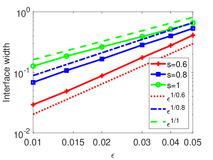
It is well-known that the parameter $\epsilon$ represents the interfacial width of the classical Allen-Cahn equation, i.e., $s=1$ , while for fractional-in-space Allen-Cahn equation the interfacial width decreases as $s$ decreases (cf. [6, 30, 28]). However, those existing work enjoys fractional-in-space Allen-Cahn equation with Riemann-Liouville fractional derivatives or spectral fractional Laplacian operator instead of the integral fractional Laplacian. As we mentioned before, different definitions of fractional Laplacian operators are very different from each other. In this example, we take the initial condition to be $u_{0}(x)=1$ if $x\in(-2,2)$ and $u_{0}(x)=0$ on $\Omega\backslash(-2,2)$ , where $\Omega=(-10,10)$ . The other parameters are $T=100$ , $\tau=10^{-2}$ , and degree of freedom $N=2^{12}$ . We plot interfacial layer with various $\epsilon$ in Figure 4.5 (a), for which we take $s=0.8$ . We observe that the interfacial layer is smoother for larger $\epsilon$ . We then present in Figure 4.5 (b) the interfacial width with various $\epsilon$ and $s$ . Here, the interfacial width is calculated by the distance of two points where $u(x,T)$ first exceeds $0.01$ and $0.99$ . We observe from Figure 4.5 (b) that interfacial width increases as $s$ increases, and behaves like $O(\epsilon^{1/s})$ .

5. Concluding remarks

In this paper, we derive the explicit form of the stiffness matrix associate with the integral fractional Laplacian in the frequency space, which is extendable to multi-dimensional rectangular elements. Then we give a complete answer to the question on when the stiffness matrix can be strictly diagonally dominant. As an application, we consider the fractional-in-space Allen-Cahn equation and show that it satisfies the maximum principle and energy dissipation law at the continuous level. Then, we proposed two full-discrete schemes using the semi-implicit and Crank-Nicolson scheme in time and modified FEM in space, which can preserve these two properties. Our numerical experiments demonstrate that our algorithms are efficient and accurate. We also observe some interesting phenomena related to the transition of the model when the fractional order $s\in(s_{0},1)$ varies to $s=1$ . For example, the width of the interfacial layer behaves like $O(\epsilon^{1/s}),$ and the decay of the solution in space obeys certain power law as reported earlier.

Appendix A Proof of Theorem 2.1

Using (2.3b) and Lemma 2.1, we obtain from direct calculation and a change of variable that

\begin{split}S_{kj}&=\frac{2}{\pi h^{2}}\int_{\mathbb{R}}|\xi|^{2s}\cos((k-j)h\xi)\Big(\frac{1-\cos(h\xi)}{\xi^{2}}\Big)^{2}\,{\rm d}\xi\\ &=\frac{4}{\pi h^{2}}\int_{0}^{\infty}\xi^{2s}\cos((k-j)h\xi)\Big(\frac{1-\cos(h\xi)}{\xi^{2}}\Big)^{2}\,{\rm d}\xi\\ &=\frac{4}{\pi h^{2s-1}}\int_{0}^{\infty}y^{2s-4}\cos(|k-j|y)(1-\cos y)^{2}\,{\rm d}y,\end{split}

(A.1)

which implies the entry $S_{kj}$ only depends on $p=|k-j|,$ so the matrix $\bm{S}$ is a symmetric Toeplitz matrix. We intend to explicitly evaluate the integral (A.1). From the fundamental trigonometric identities, we find readily that

\begin{split}f(y;p)&:=\cos(py)(1-\cos y)^{2}=\cos(py)\Big(\frac{3}{2}-2\cos y+\frac{1}{2}\cos(2y)\Big)\\ &=\frac{1}{4}\sum_{i=-2}^{2}c_{i}\cos(|p+i|y).\end{split}

(A.2)

We continue the calculation by using integration by parts. The number of times that we can integrate by parts depends on the range of $s,$ so we proceed with three cases with $s\in(1,\frac{3}{2}),(\frac{1}{2},1)$ and $(0,\frac{1}{2}),$ separately. Then we derive the formulas for $s=\frac{1}{2},1$ by taking limits.

Case (i) $s\in(1,\frac{3}{2})$ : Recall the integral identity (cf. [17, P. 440]):

\int^{\infty}_{0}x^{\mu-1}\sin(ax)\,{\rm d}x=\frac{\Gamma(\mu)}{a^{\mu}}\sin\Big(\frac{\mu\pi}{2}\Big),\quad a>0,\;\;\mu\in(0,1).

(A.3)

We derive from (A.1) and integration by parts immediately that

\int_{0}^{\infty}y^{2s-4}f(y;p){\rm d}y=-\frac{1}{2s-3}\int_{0}^{\infty}y^{2s-3}f^{\prime}(y;p){\rm d}y.

(A.4)

By (A.2), we obtain from (A.3) with $\mu=2s-2\in(0,1)$ that

\begin{split}\int_{0}^{\infty}y^{2s-3}&f^{\prime}(y;p){\rm d}y=-\frac{1}{4}\int_{0}^{\infty}y^{2s-3}\big\{|p-2|\sin(|p-2|y)-4|p-1|\sin(|p-1|y)\\ &\quad+6p\sin(py)-4(p+1)\sin((p+1)y)+(p+2)\sin((p+2)y)\big\}{\rm d}y\\ &=-\frac{\Gamma(2s-2)}{4}\sin\big((s-1)\pi\big)\big\{|p-2|^{3-2s}-4|p-1|^{3-2s}+6p^{3-2s}\\ &\quad-4(p+1)^{3-2s}+(p+2)^{3-2s}\big\}.\end{split}

(A.5)

Thus, we infer from (A.1)-(A.2) and (A.4)-(A.5) that

\begin{split}S_{kj}&=\frac{1}{\pi h^{2s-1}}\frac{1}{2s-3}\int_{0}^{\infty}y^{2s-3}f^{\prime}(y;p)\,{\rm d}y=-\frac{\sin\big(s\pi\big)\;\Gamma(2s-3)}{\pi h^{2s-1}}t_{p}.\end{split}

Then we have the entries of $\bm{S}$ with $s\in(1,\frac{3}{2})$ by using the reflection property (cf. [24, P. 138]):

\Gamma(z)\Gamma(1-z)=\frac{\pi}{\sin\pi z},\quad z\not=0,-1,-2,\cdots.

(A.6)

Case (ii) $s\in(\frac{1}{2},1)$ : In this case, we can integrate (A.4) by parts one more time, and then use the identity (cf. [17, P. 441]):

\int^{\infty}_{0}x^{\mu-1}\cos(ax)\,{\rm d}x=\frac{\Gamma(\mu)}{a^{\mu}}\cos\Big(\frac{\mu\pi}{2}\Big),\quad a>0,\;\;\;\mu\in(0,1).

(A.7)

More precisely, by (A.4) and (A.7) with $\mu=2s-1\in(0,1),$

\begin{split}&\int_{0}^{\infty}y^{2s-4}f(y;p){\rm d}y=\frac{1}{(2s-3)(2s-2)}\int_{0}^{\infty}y^{2s-2}f^{\prime\prime}(y;p){\rm d}y\\ &=-\frac{1}{4(2s-3)(2s-2)}\int_{0}^{\infty}y^{2s-2}\big\{|p-2|^{2}\cos(|p-2|y)-4|p-1|^{2}\cos(|p-1|y)\\ &\quad+6p^{2}\cos(py)-4(p+1)^{2}\cos((p+1)y)+(p+2)^{2}\cos((p+2)y)\big\}{\rm d}y\\ &=-\frac{\Gamma(2s-3)}{4}\cos\Big(\frac{(2s-1)\pi}{2}\Big)t_{p}.\end{split}

(A.8)

Hence, by (A.1) and (A.6),

\begin{split}&S_{kj}=\frac{4}{\pi h^{2s-1}}\int_{0}^{\infty}y^{2s-4}f(y;p)\,{\rm d}y=-\frac{\sin(s\pi)\;\Gamma(2s-3)}{\pi h^{2s-1}}t_{p}=\frac{\sec(s\pi)}{2h^{1-2s}\Gamma(4-2s)}t_{p},\end{split}

(A.9)

which yields the desired formula with $s\in(\frac{1}{2},1).$

Case (iii) $s\in(0,\frac{1}{2})$ : Similarly, we integrate the first equality of (A.8) by parts one more time and obtain

\begin{split}\int_{0}^{\infty}y^{2s-4}f(y;p){\rm d}y&=-\frac{1}{(2s-3)(2s-2)(2s-1)}\int_{0}^{\infty}y^{2s-1}f^{\prime\prime\prime}(y;p)\,{\rm d}y,\end{split}

(A.10)

which involves sines, so we use (A.3) with $\mu=2s\in(0,1)$ to evaluate the integrals. Then following the same lines as the previous case, we can derive the entries with $s\in(0,\frac{1}{2})$ in a similar fashion.

Case (iv) $s=\frac{1}{2}$ : Observe from (2.3b) that $S_{kj}$ continuously depends on the parameter $s.$ We can compute the entries by taking the limit

S_{kj}=\frac{1}{4}\lim_{s\to\frac{1}{2}}\frac{t_{p}}{\cos(s\pi)},

(A.11)

and resort to the basic limit

\ln z=\lim_{\epsilon\rightarrow 0}\frac{z^{\epsilon}-1}{\epsilon},\ \ z>0,

(A.12)

which is a direct consequence of the L’Hospital’s rule. Note that

\sum_{i=-2}^{2}c_{i}(p+i)^{l}=0,\quad l=0,1,2,

(A.13)

so we can rewrite the entries in (2.6) for $p=|k-j|\geq 3$ as

\begin{split}S_{kj}&=\frac{1}{4}\lim_{s\to\frac{1}{2}}\frac{1-2s}{\cos(s\pi)}\sum_{i=-2}^{2}c_{i}\lim_{s\to\frac{1}{2}}\frac{|p+i|^{3-2s}-(p+i)^{2}}{1-2s}\\ &=\frac{1}{2\pi}\sum_{i=-2}^{2}c_{i}(p+i)^{2}\lim_{s\to\frac{1}{2}}\frac{|p+i|^{1-2s}-1}{1-2s}=\frac{1}{2\pi}\sum_{i=-2}^{2}c_{i}(p+i)^{2}\ln|p+i|.\end{split}

(A.14)

Note that for $p=0,1,2$ and $p+i=0$ , the formula still holds with the understanding of $(p+i)^{2}\ln|p+i|=0$ . This leads to (2.7).

(v). Case $s=1$ : In this case, we directly take the limit upon (2.6), and find readily that

S_{kj}=-\frac{t_{p}}{2h}\Big|_{s=1}=\frac{1}{h}\begin{cases}{2,}&{j=k},\\ {-1,}&{j=k\pm 1},\\ {0,}&{\text{ otherwise. }}\end{cases}

(A.15)

This yields the stiffness matrix of the usual 1D Laplacian as expected.

References

[1] G. Acosta, F.M. Bersetche, and J.P. Borthagaray. A short FE implementation for a 2d homogeneous Dirichlet problem of a fractional Laplacian. Comput. Math. Appl., 74(4):784–816, 2017.
[2] M. Ainsworth and C. Glusa. Towards an efficient finite element method for the integral fractional Laplacian on polygonal domains. In Contemporary computational mathematics—a celebration of the 80th birthday of Ian Sloan. Vol. 1, 2, pages 17–57. Springer, Cham, 2018.
[3] A.S. Alfa, J.G. Xue, and Q. Ye. Accurate computation of the smallest eigenvalue of a diagonally dominant $M$ -matrix. Math. Comp., 71(237):217–236, 2002.
[4] I. Babuška, T. Strouboulis, et al. The finite element method and its reliability. Oxford university press, 2001.
[5] A. Bueno-Orovio, D. Kay, and K. Burrage. Fourier spectral methods for fractional-in-space reaction-diffusion equations. BIT Numer. Math., 54(4):937–954, 2014.
[6] K. Burrage, N. Hale, and D. Kay. An efficient implicit FEM scheme for fractional-in-space reaction-diffusion equations. SIAM J. Sci. Comput., 34(4):A2145–A2172, 2012.
[7] Q. Du and X.B. Feng. The phase field method for geometric moving interfaces and their numerical approximations. In Handbook of Numerical Analysis, volume 21, pages 425–508. Elsevier, 2020.
[8] Q. Du, J. Yang, and Z. Zhou. Time-fractional Allen-Cahn equations: Analysis and numerical methods. arXiv:1906.06584, 2019.
[9] S.W. Duo, H.W. van Wyk, and Y.Z. Zhang. A novel and accurate finite difference method for the fractional Laplacian and the fractional poisson problem. J. Comput. Phys., 355:233–252, 2018.
[10] S.W. Duo and H. Wang. A fractional phase-field model using an infinitesimal generator of $\alpha$ stable Lévy process. J. Comput. Phys., 384:253–269, 2019.
[11] S.W. Duo and Y.Z. Zhang. Accurate numerical methods for two and three dimensional integral fractional Laplacian with applications. Comput. Methods Appl. Mech. Eng., 355:639–662, 2019.
[12] A. Erdélyi, W. Magnus, F. Oberhettinger, and F.G. Tricomi. Higher transcendental functions. Vol. I. Robert E. Krieger Publishing Co., Inc., Melbourne, Fla., 1981. Based on notes left by Harry Bateman, With a preface by Mina Rees, With a foreword by E. C. Watson, Reprint of the 1953 original.
[13] F.O. Farid. Notes on matrices with diagonally dominant properties. Linear Algebra Appl., 435(11):2793–2812, 2011.
[14] X.B. Feng and A. Prohl. Numerical analysis of the Allen-Cahn equation and approximation for mean curvature flows. Numer. Math., 94(1):33–65, 2003.
[15] A. George and K.D. Ikramov. Gaussian elimination is stable for the inverse of a diagonally dominant matrix. Math. Comp., 73(246):653–657, 2004.
[16] G.H. Golub and C.F. Van Loan. Matrix Computations. Johns Hopkins Studies in the Mathematical Sciences. Johns Hopkins University Press, Baltimore, MD, third edition, 1996.
[17] I.S. Gradshteyn and I.M. Ryzhik. Table of Integrals, Series, and Products. Elsevier/Academic Press, Amsterdam, eighth edition, 2015. Translated from the Russian, Translation edited and with a preface by Daniel Zwillinger and Victor Moll, Revised from the seventh edition [MR2360010].
[18] R.A. Horn and C.R. Johnson. Matrix Analysis. Cambridge University Press, Cambridge, 1985.
[19] T.L. Hou, T. Tang, and J. Yang. Numerical analysis of fully discretized Crank–Nicolson scheme for fractional-in-space Allen–Cahn equations. J. Sci. Comput., 72(3):1214–1231, 2017.
[20] Y.K. Li. Numerical methods for deterministic and stochastic phase field models of phase transition and related geometric flows (Ph.D. thesis). University of Tennessee, 2015.
[21] Z. Li, H. Wang, and D.P. Yang. A space–time fractional phase-field model with tunable sharpness and decay behavior and its efficient numerical simulation. J. Comput. Phys., 347:20–38, 2017.
[22] H.L. Liao, T. Tang, and T. Zhou. A second-order and nonuniform time-stepping maximum-principle preserving scheme for time-fractional Allen-Cahn equations. J. Comput. Phys., 414:109473, 2020.
[23] H. Liu, A.J. Cheng, H. Wang, and J. Zhao. Time-fractional Allen–Cahn and Cahn–Hilliard phase-field models and their numerical investigation. Comput. Math. Appl., 76(8):1876–1892, 2018.
[24] F.W.J. Olver, D.W. Lozier, R.F. Boisvert, and C.W. Clark, editors. NIST Handbook of Mathematical Functions. U.S. Department of Commerce, National Institute of Standards and Technology, Washington, DC; Cambridge University Press, Cambridge, 2010. With 1 CD-ROM (Windows, Macintosh and UNIX).
[25] A. Quarteroni and A. Valli. Numerical Approximation of Partial Differential Equations, volume 23 of Springer Series in Computational Mathematics. Springer-Verlag, Berlin, 1994.
[26] J. Shen, T. Tang, and L.L. Wang. Spectral Methods: Algorithms, Analysis and Applications, volume 41 of Series in Computational Mathematics. Springer-Verlag, Berlin, Heidelberg, 2011.
[27] J. Shen, J. Xu, and J. Yang. A new class of efficient and robust energy stable schemes for gradient flows. SIAM Rev., 61(3):474–506, 2019.
[28] C.T. Sheng, D. Cao, and J. Shen. Efficient spectral methods for PDEs with spectral fractional Laplacian. Submitted, 2020.
[29] C.T. Sheng, J. Shen, T. Tang, L.L. Wang, and H.F. Yuan. Fast Fourier-like mapped Chebyshev spectral-Galerkin methods for PDEs with integral fractional Laplacian in unbounded domains. Accepted by SIAM J. Numer. Anal., 2020.
[30] F.Y. Song, C.J. Xu, and G. E. Karniadakis. A fractional phase-field model for two-phase flows with tunable sharpness: Algorithms and simulations. Comput. Methods Appl. Mech. Engrg., 305:376–404, 2016.
[31] T. Tang. Revisit of semi-implicit schemes for phase field equation. arXiv:2006.06990, 2020.
[32] T. Tang and J. Yang. Implicit-explicit scheme for the Allen-Cahn equation preserves the maximum principle. J. Comput. Math., 34(5):471–481, 2016.
[33] T. Tang, H.J. Yu, and T. Zhou. On energy dissipation theory and numerical stability for time-fractional phase-field equations. SIAM J. Sci. Comput., 41(6):A3757–A3778, 2019.
[34] W.Y. Tian, H. Zhou, and W.H. Deng. A class of second order difference approximations for solving space fractional diffusion equations. Math. Comp., 84(294):1703–1727, 2015.
[35] A. Tveito and R. Winter. Introduction to Partial Differential Equations, volume 29 of Texts in Applied Mathematics. Springer-Verlag, Berlin, 2009. A Computational Approach, Paperback reprint of the 2005 edition.
[36] T.J. Urekew and J.J. Rencis. The importance of diagonal dominance in the iterative solution of equations generated from the boundary element method. Int. J. Numer. Meth. Eng., 36(20):3509–3527, 1993.
[37] F. Wang, H. Chen, and H. Wang. Finite element simulation and efficient algorithm for fractional Cahn–Hilliard equation. J. Comput. Appl. Math., 356:248–266, 2019.
[38] J.C. Xu, Y.K. Li, S.N. Wu, and A. Bousquet. On the stability and accuracy of partially and fully implicit schemes for phase field modeling. Comput. Methods Appl. Mech. Eng., 345:826–853, 2019.
[39] J. Zhao, L.Z. Chen, and H. Wang. On power law scaling dynamics for time-fractional phase field models during coarsening. Commun. Nonlinear Sci. Numer. Simul., 70:257–270, 2019.