Dark matter physics in dark $SU(2)$ gauge symmetry
with non-Abelian kinetic mixing

The standard model (SM) of particle physics has been very successful in describing phenomenology observed in various experiments. However the existence of dark matter (DM) cannot be explained in the SM framework, and it would be described as a new particle associated with physics beyond the SM. The nature of DM is an open question and there are many experimental searches for interactions among DM and the SM particles such as in direct detection, indirect detection and collider experiments. No clear evidence of DM would indicate a dark sector which is hidden from current observations.

As the SM is described by local gauge symmetries, it is plausible that the dark sector is also ruled by a hidden/dark gauge symmetry. Moreover stability of DM indicates necessity of a symmetry to protect it from decay, and it can be a remnant of dark gauge symmetry (see Ref. Ko:2018qxz for a review along this line). Thus, it is an attractive scenario that dark gauge symmetry is spontaneously broken to a symmetry stabilizing DM candidate. To realize this concept, we are especially interested in the extension of the SM introducing a new $SU(2)_{D}$ gauge symmetry where all the SM fields are singlet under it. The interesting properties of a model with local $SU(2)_{D}$ group is that an unbroken discrete symmetry can be naturally preserved after the spontaneous breaking of the $SU(2)_{D}$ gauge symmetry comparing with a hidden local $U(1)$ case in which the $U(1)$ charge has to satisfy some artificial tuning Krauss:1988zc. Note that various applications of the hidden $SU(2)$ gauge symmetry have been studied in literatures, for examples, a remaining $Z_{3}(Z_{4})$ symmetry with a quadruplet(quintet) in ref. Chiang:2013kqa; Chen:2015nea; Chen:2015dea, $Z_{2}\times Z^{\prime}_{2}$ symmetry Gross:2015cwa, a custodial symmetry in refs. Boehm:2014bia; Hambye:2008bq and an unbroken $U(1)$ from $SU(2)$ in refs. Baek:2013dwa; Khoze:2014woa; Daido:2019tbm.

In this paper, we discuss a simple scenario in which $SU(2)_{D}$ gauge symmetry is broken into discrete $Z_{2}$ symmetry by vacuum expectation values (VEVs) of two $SU(2)_{D}$ triplet real scalar fields ($\vec{\phi}$ and $\vec{\phi}^{\prime}$), and an $SU(2)_{D}$ doublet Dirac fermion $\chi$ is $Z_{2}$-odd DM candidate. We also introduce higher dimensional operators that induce gauge kinetic mixing terms between $SU(2)_{D}$ and $U(1)_{Y}$ gauge fields after $SU(2)_{D}$ symmetry breaking by nonzero VEV’s of $\vec{\phi}$ and $\vec{\phi}^{\prime}$ as mediators between the dark gauge sector and the SM sector. After fixing our model, we formulate particle mass spectra and their interactions in the dark sector and the portals to the SM sector. Then relic density of our DM candidate is estimated taking into account constraint from direct detection of DM. Furthermore we discuss implications to collider physics considering the scalar portal and the kinetic mixing as connections between dark sector and the SM.

This paper is organized as follows. In Sec. II, we show our model of $SU(2)_{D}$ dark sector formulating mass spectra and interactions. In Sec. III, we analyze DM relic density and discuss the allowed parameter region. In Sec. IV, we discuss implications to collider physics. Finally We conclude and discuss in Sec. V.

In this section we summarize the setup for our model. We introduce a dark sector which is controlled by a non-Abelian $SU(2)_{D}$ dark gauge symmetry, with two real scalar fields $\vec{\phi}$ and $\vec{\phi}^{\prime}$, and one Dirac fermion $\chi$ as summarized in Table 1. In components, $\vec{\phi}(\vec{\phi}^{\prime})$ and $\chi$ are written as

where the indices for triplet scalars correspond to three $SU(2)_{D}$ generators.

The $SU(2)_{D}$ dark gauge symmetry is spontaneously broken by nonzero VEV’s of two real scalar triplets $\phi$ and $\phi^{\prime}$. In our scenario, we assume VEV alignments of two scalar triplets as

When $SU(2)_{D}$ is broken by the VEVs of the triplets, the vacuum is invariant under the transformation defined by $U_{T_{3}}\equiv e^{i2\pi T_{3}}$ as $U_{T_{3}}\langle\vec{\phi}^{(\prime)}\rangle=\langle\vec{\phi}^{(\prime)}\rangle$, where $T_{3}$ is the diagonal component of $SU(2)_{D}$ generators. Then $\chi$ field transform $U_{T_{3}}\chi=-\chi$ since $T_{3}$ values of $\chi$’s components are $\pm 1/2$. In general, we would obtain even (odd) parity under $U$ transformation for any component of $SU(2)_{D}$ multiplet with integer (half-integer) value of $T_{3}$. Thus $SU(2)_{D}$ gauge symmetry is broken to $Z_{2}$ symmetry when we assume Eq. (II.2). Note that the $Z_{2}$ symmetry will guarantees the stability of DM candidate which is the lightest component with odd $Z_{2}$ parity.

Now we write down the Lagrangian for kinetic terms of the dark sector and the scalar potential:

where $X_{\mu\nu}^{a}(a=1,2,3)$ is the field strength of $SU(2)_{D}$ gauge field, and $H$ is the SM Higgs doublet field written as

Here $v_{H}$ is the VEV of the SM Higgs doublet, $H$, and $G^{\pm}$ and $G_{Z}$ are Nambu-Goldstone(NG) bosons absorbed by $W^{\pm}$ and $Z$ bosons.

In this section, we discuss DM phenomenology in our model including DM relic density. In our scenario, DM is the lightest lightest dark fermion $\chi_{l}$ which is stabilized by the remnant dark $Z_{2}$ symmetry after dark gauge symmetry breaking. Firstly we require that Higgs portal interactions of DM are suppressed in order to avoid severe constraints from DM direct detection experiments. For the scenario (1) of Higgs mixing, we prefer large mixing of dark fermions, $\theta_{\chi}\sim\pi/4$, since DM couples with Higgs via $\phi_{3}$. On the other hand, for the scenario (2), we prefer small mixing, $|\theta_{\chi}|<<1$, since DM couples with Higgs via $\phi^{\prime}_{1}$. Then relic density of DM is determined by gauge interactions in dark sector in our scenarios where we assume dark scalars are heavier than DM.

Then, the relevant interaction terms are

where $J_{EM}^{\mu}$ is electromagnetic current and $Q_{f_{SM}}$ is the electric charge of the SM fermions $f_{SM}$. Then we implement these interactions in micrOMEGAs 4.3.5 Belanger:2014vza to estimate relic density.

In our analysis we take the dark fermion mixing angle for each scenario as

in order to avoid direct detection constraint. For illustration, we consider two benchmark cases of dark gauge boson masses for each scenario;

and $m_{X_{2}}=\sqrt{m^{2}_{X_{1}}+m^{2}_{X_{3}}}$. Also we require interaction between DM and the lightest dark gauge boson not to be suppressed by the dark fermion mixing effect. In the following, we shall focus on the scenario (1) since we just obtain similar results by replacing the role of $X_{1}$ and $X_{3}$ for the scenario (2).

In addition, we take into account $DM$-nucleon scattering via $Z^{\prime}$ boson exchanging process. The cross section for this process is calculated in non-relativistic limit as

where $m_{p}$ indicates the proton mass. Since the $Z^{\prime}$-SM fermion interaction is proportional to electromagnetic current, the DM scattering with neutron is suppressed. For $m_{\chi_{l}}=\mathcal{O}(100)$ GeV, we obtain

We then assume $\delta_{1}\lesssim 10^{-5}$ to avoid direct detection constraints such as XENON1T Aprile:2018dbl and PandaX-II Cui:2017nnn which provide upper limit of $\sim 10^{-46}$ cm² for DM mass of $\sim 100$ GeV.

In Fig. 1, we show thermal relic density of DM, adopting dark gauge boson masses $\{m_{X_{1}},m_{X_{3}}\}$ as $\{200,500\}$ GeV and $\{10,30\}$ GeV as reference values, $m_{\chi_{h}}=1.5m_{\chi_{l}}$, $\delta_{1,3}=10^{-5}$, and some relevant values of gauge coupling $g_{D}$. We find that relic density is decreased when $\chi_{l}\bar{\chi}_{l}\to X_{1}X_{1}$ and $\chi_{l}\bar{\chi}_{l}\to X_{2}X_{2}$ processes are kinematically allowed. Then larger gauge coupling is required for larger $m_{X_{1}}$ mass to accommodate with observed thermal relic density of DM. We can also explain relic density around resonance $2m_{X_{\chi_{l}}}\sim m_{X_{1}}$ when $X_{1}$ mass is relatively light while the relic density tends to be larger than observed one for heavier dark gauge boson case due to small kinetic mixing parameter.

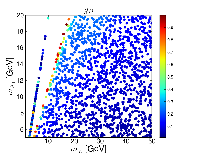
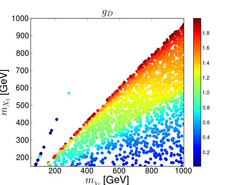
Next we scan free parameters fixing ${\delta_{1,3}}=10^{-5}$ to avoid direct detection constraint. The two region for masses of $\chi_{l,h}$ and $X_{1,3}$ are considered in the range of

where masses of $\chi_{h}$ and $X_{3}$ are respectively determined by those of $\chi_{l}$ and $X_{1}$ for simplicity. We then search for the parameter region which provide observed DM thermal relic density approximately in the range of $0.11<\Omega h^{2}<0.13$. In the left and right panels of Fig. 2, we show allowed parameter region on $\{m_{DM},m_{X_{1}}\}$ plane for the region I and II where color gradient indicates values of $g_{D}$. We find large allowed region when $\chi_{l}\bar{\chi}_{l}\to X_{1}X_{1}(X_{2}X_{2})$ processes are kinematically allowed. On the other hand, for $m_{X_{1}}>m_{\chi_{l}}$, we need some fine tuning around $m_{X_{1}}\simeq 2m_{\chi_{l}}$ to obtain resonant enhancement of annihilation cross section.

Here we discuss collider physics in the model focusing extra scalar boson production at the LHC via Higgs mixing. Then extra scalar boson decays into dark gauge boson, dark fermion or SM particles where the branching ratio (BR) depend on parameters in the model. We then discuss possible signals of the model at the LHC.

References

• (1) P. Ko, J. Korean Phys. Soc. 73, no.4, 449-465 (2018) doi:10.3938/jkps.73.449
• (2) L.M. Krauss and F. Wilczek, Phys. Rev. Lett. 62, 1221 (1989).
• (3) C. W. Chiang, T. Nomura and J. Tandean, JHEP 1401, 183 (2014) [arXiv:1306.0882 [hep-ph]].
• (4) C. H. Chen and T. Nomura, Phys. Lett. B 746, 351 (2015) [arXiv:1501.07413 [hep-ph]].
• (5) C. H. Chen and T. Nomura, Phys. Rev. D 93, no. 7, 074019 (2016) [arXiv:1507.00886 [hep-ph]].
• (6) C. Gross, O. Lebedev and Y. Mambrini, JHEP 1508, 158 (2015) [arXiv:1505.07480 [hep-ph]].
• (7) T. Hambye, JHEP 0901, 028 (2009) [arXiv:0811.0172 [hep-ph]].
• (8) C. Boehm, M. J. Dolan and C. McCabe, Phys. Rev. D 90, no. 2, 023531 (2014) [arXiv:1404.4977 [hep-ph]].
• (9) S. Baek, P. Ko and W. I. Park, JCAP 1410, 067 (2014) [arXiv:1311.1035 [hep-ph]].
• (10) V. V. Khoze and G. Ro, JHEP 1410, 61 (2014) [arXiv:1406.2291 [hep-ph]].
• (11) R. Daido, S. Y. Ho and F. Takahashi, JHEP 2001, 185 (2020) [arXiv:1909.03627 [hep-ph]].
• (12) S. Choi, S. Jung and P. Ko, JHEP 1310, 225 (2013) [arXiv:1307.3948 [hep-ph]].
• (13) K. Cheung, P. Ko, J. S. Lee and P. Y. Tseng, JHEP 1510, 057 (2015) [arXiv:1507.06158 [hep-ph]].
• (14) C. A. Argüelles, X. G. He, G. Ovanesyan, T. Peng and M. J. Ramsey-Musolf, Phys. Lett. B 770, 101 (2017) [arXiv:1604.00044 [hep-ph]].
• (15) E. J. Weinberg, doi:10.1017/CBO9781139017787
• (16) G. Belanger, F. Boudjema, A. Pukhov and A. Semenov, Comput. Phys. Commun. 192, 322 (2015) [arXiv:1407.6129 [hep-ph]].
• (17) X. Cui et al. [PandaX-II Collaboration], Phys. Rev. Lett. 119, no. 18, 181302 (2017) [arXiv:1708.06917 [astro-ph.CO]].
• (18) E. Aprile et al. [XENON Collaboration], Phys. Rev. Lett. 121, no. 11, 111302 (2018) [arXiv:1805.12562 [astro-ph.CO]].
• (19) M. Aaboud et al. [ATLAS Collaboration], JHEP 1806, 166 (2018) [arXiv:1802.03388 [hep-ex]].
• (20) J. F. Gunion, H. E. Haber, G. L. Kane and S. Dawson, Front. Phys. 80, 1 (2000).