跳到论文正文
W Papers独立论文阅读器 arXiv:2007.08110 论文正文 计算阅读时间 · 0%
引用这篇论文根据当前论文元数据生成,正式投稿前建议核对。


License: arXiv.org perpetual non-exclusive license
arXiv:2007.08110v2 [cs.DS] 17 Jul 2020

Private Approximations of a Convex Hull in Low Dimensions

Yue Gao Thanks: Y.G.˜gratefully acknowledges funding from the Natural Sciences and Engineering Research Council of Canada (NSERC) and from the Alberta Machine Intelligence Institute (Amii). Affiliation: Dept. of Computing Science Affiliation: University of Alberta Affiliation: Edmonton, AB Canada Email: gao12@ualberta.ca    Or Sheffet Thanks: O.S.˜gratefully acknowledges the Natural Sciences and Engineering Research Council of Canada (NSERC) for supporting O.S.˜with grant #2017–06701, which also helped fund Y.G.˜when she was advised by O.S.˜at the University of Alberta. Much of this work was done when O.S.˜was a visitor at the “Data Privacy: Foundations and Application” program held in spring 2019 at the Simons Institute for the Theory of Computing, UC Berkeley. Affiliation: Faculty of Engineering Affiliation: Bar-Ilan University Affiliation: Ramat-Gan, Israel Email: or.sheffet@biu.ac.il

We give the first differentially private algorithms that estimate a variety of geometric features of points in the Euclidean space, such as diameter, width, volume of convex hull, min-bounding box, min-enclosing ball etc. Our work relies heavily on the notion of Tukey-depth. Instead of (non-privately) approximating the convex-hull of the given set of points PP, our algorithms approximate the geometric features of the κ\kappa-Tukey region induced by PP (all points of Tukey-depth κ\kappa or greater). Moreover, our approximations are all bi-criteria: for any geometric feature μ\mu our (α,Δ)(\alpha,\Delta)-approximation is a value “sandwiched” between (1−α)​μ​(DP​(κ))(1-\alpha)\mu(D_{P}(\kappa)) and (1+α)​μ​(DP​(κ−Δ))(1+\alpha)\mu(D_{P}(\kappa-\Delta)).

Our work is aimed at producing a (α,Δ)(\alpha,\Delta)-kernel of DP​(κ)D_{P}(\kappa), namely a set 𝒮\mathcal{S} such that (after a shift) it holds that (1−α)​DP​(κ)⊂𝖢𝖧⁡(𝒮)⊂(1+α)​DP​(κ−Δ)(1-\alpha)D_{P}(\kappa)\subset\mathsf{CH}(\mathcal{S})\subset(1+\alpha)D_{P}(\kappa-\Delta). We show that an analogous notion of a bi-critera approximation of a directional kernel, as originally proposed by [AHV04], fails to give a kernel, and so we result to subtler notions of approximations of projections that do yield a kernel. First, we give differentially private algorithms that find (α,Δ)(\alpha,\Delta)-kernels for a “fat” Tukey-region. Then, based on a private approximation of the min-bounding box, we find a transformation that does turn DP​(κ)D_{P}(\kappa) into a “fat” region but only if its volume is proportional to the volume of DP​(κ−Δ)D_{P}(\kappa-\Delta). Lastly, we give a novel private algorithm that finds a depth parameter κ\kappa for which the volume of DP​(κ)D_{P}(\kappa) is comparable to DP​(κ−Δ)D_{P}(\kappa-\Delta). We hope this work leads to the further study of the intersection of differential privacy and computational geometry.

1 Introduction

With modern day abundance of data, there are numerous datasets that hold the sensitive and personal details of individuals, yet collect only a few features per user. Examples of such low-dimensional datasets include locations (represented as points on the 2​D2D-plane), medical data composed of only a few measurements (e.g. [SFIW17, WYH19]), or high-dimensional data restricted to a small subset of features (often selected for the purpose of data-visualization). It is therefore up to us to make sure that the analyses of such sensitive datasets do not harm the privacy of their participants. Differentially private algorithms [DMNS06, DKM+06] alleviate such privacy concerns as they guarantee that the presence or absence of any single individual in the dataset has only a limited affect on any outcome.

Often (again, commonly motivated by visualization), understanding the geometric features of such low-dimensional datasets is a key step in their analysis. Yet, to this day, very little work has been done to establish differentially private algorithms that approximate the data’s geometrical features. This should not come as a surprise seeing as most geometric features --- such as diameter, width,11 1 The min gap between two hyperplanes that “sandwich” the data. volume of convex-hull, min-bounding ball radius, etc. — are highly sensitive to the presence / absence of a single datum. Moreover, while it is known that differential privacy generalizes [DFH+15, BNS+16], geometrical properties often do not: if the dataset PP is composed on nn i.i.d draws from a distribution 𝒫\mathcal{P} then it might still be likely that, say, diam⁡(P)\mathrm{diam}(P) and diam⁡(𝒫)\mathrm{diam}(\mathcal{P}) are quite different.22 2 For example, consider 𝒫\mathcal{P} as a uniform distribution over 2​n2n discrete points whose diameter greatly shrinks unless two specific points are drawn into PP.

But differential privacy has already overcome the difficulty of large sensitivity in many cases, the leading example being the median — despite the fact that the median may vary greatly with the addition of a new entry into the data, we are still capable of privately approximating the median. The crux in differentially private median approximation is that the quality of the approximation is not measured by the actual distance between the true input-median and the result of the algorithm, but rather by the probability mass of the input’s CDF “sandwiched” between the true median and the output of the private algorithm. A similar effect takes place in our work. While we deal with geometric concepts that exhibit large sensitivity, we formulate robust approximation guarantees of these concepts, guarantees that do generalize when the data is drawn i.i.d. from some unknown distribution. And much like in previous works in differential privacy [BMNS19, KSS20], our approximation rely heavily on the notion of the depth of a point.

Specifically, our approximation guarantees are with respect to Tukey depth [TUK75]. Roughly speaking (see Section 2), a point xx has Tukey depth κ\kappa w.r.t. a dataset PP, denoted TD⁡(x,P)=κ\mathrm{TD}(x,P)=\kappa, if the smallest set S⊂PS\subset P one needs to remove from PP so that some hyperplane separates xx from P∖SP\setminus S has cardinality κ\kappa. This also allows us to define the κ\kappa-Tukey region DP​(κ)={x∈ℝd:TD⁡(x,P)≥κ}D_{P}(\kappa)=\{x\in\mathbb{R}^{d}:~\mathrm{TD}(x,P)\geq\kappa\}. So, for example, DP​(0)=ℝdD_{P}(0)=\mathbb{R}^{d} and DP​(1)=𝖢𝖧​(P)D_{P}(1)=\mathsf{CH}(P) (the convex-hull of PP). It follows from the definition that for any 1≤κ1≤κ21\leq\kappa_{1}\leq\kappa_{2} we have 𝖢𝖧⁡(P)=DP​(1)⊃DP​(κ1)⊃DP​(κ2)\mathsf{CH}(P)=D_{P}(1)\supset D_{P}(\kappa_{1})\supset D_{P}(\kappa_{2}). It is known that for any dataset PP and depth κ\kappa the Tukey-region DP​(κ)D_{P}(\kappa) is a convex polytope, and moreover (see [Ede87]) that for any PP of size nn it holds that DP​(n/(d+1))≠∅D_{P}(n/(d+1))\neq\emptyset. Moreover, there exists efficient algorithms (in low-dimensions) that find DP​(κ)D_{P}(\kappa).

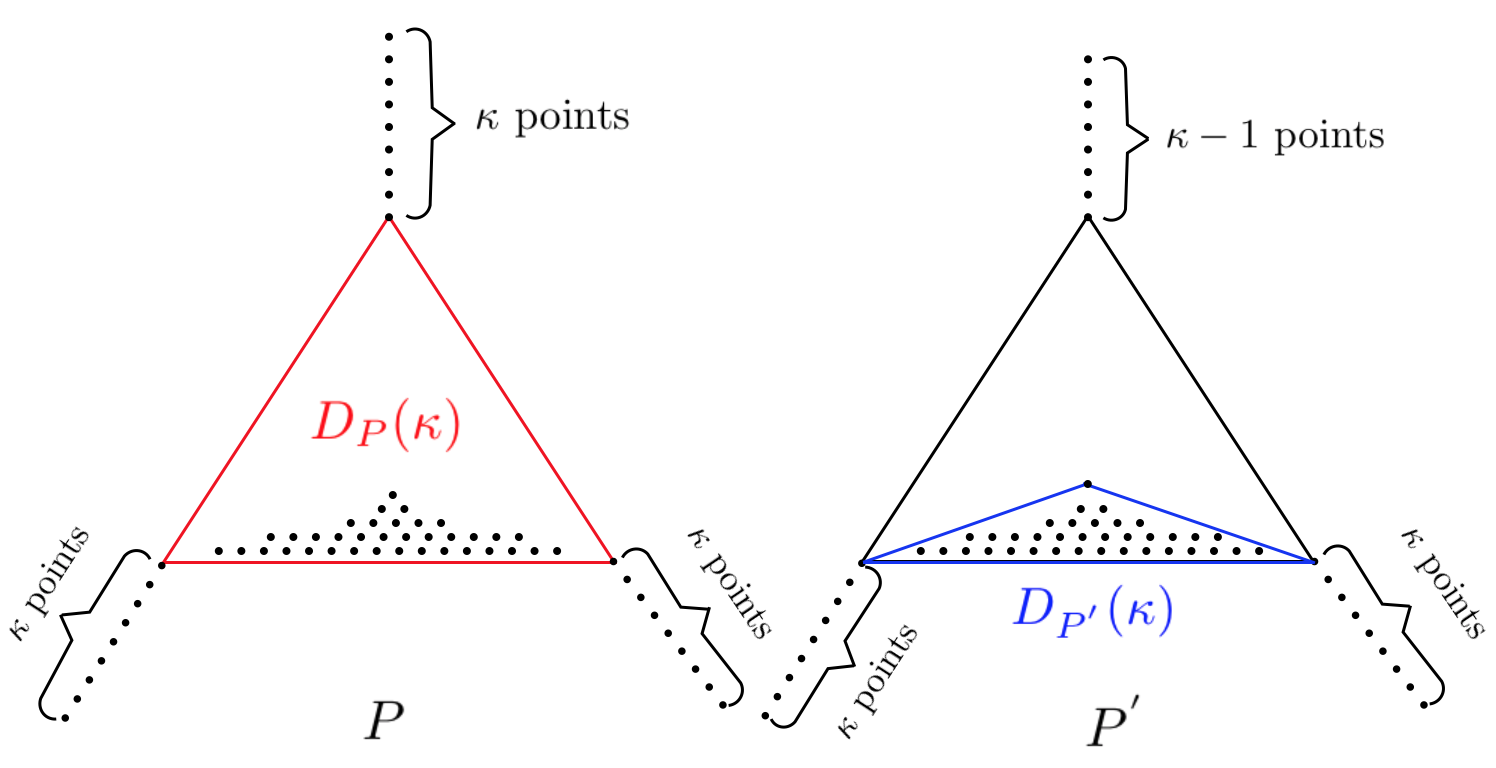
One property of the Tukey depth, a pivotal property that enables differentially private approximations, is that it exhibits low-sensitivity at any given point. As noted by [BMNS19], it follows from the very definition of Tukey-depth that if we add or remove any single datapoint to/from PP, then the depth of any given x∈ℝdx\in\mathbb{R}^{d} changes by no more than 11. And so, in this work, we give bi-criteria approximations of key geometric features of DP​(κ)D_{P}(\kappa) — where the quality of the approximation is measured both by a multiplicative factor and with respect to a shallower Tukey region. Given a measure μ\mu of the convex polytope DP​(κ)D_{P}(\kappa), such as diameter, width, volume etc., we return a (α,Δ)(\alpha,\Delta)-approximation of μ\mu — a value lower bounded by (1−α)​μ​(DP​(κ))(1-\alpha)\mu(D_{P}(\kappa)) and upper-bounded by (1+α)​μ​(DP​(κ−Δ))(1+\alpha)\mu(D_{P}(\kappa-\Delta)). This implies that the quality of the approximation depends on both the approximation parameters fed into the algorithm and also on the “niceness” properties of the data. For datasets where μ⁡(DP​(κ−Δ))≈μ⁡(DP​(κ))\mu(D_{P}(\kappa-\Delta))\approx\mu(D_{P}(\kappa)), our (α,Δ)(\alpha,\Delta)-approximation is a good approximation of μ​(DP​(κ))\mu(D_{P}(\kappa)), but for datasets where μ⁡(DP​(κ−Δ))≫μ⁡(DP​(κ))\mu(D_{P}(\kappa-\Delta))\gg\mu(D_{P}(\kappa)) our guarantee is rather weak. Note that no differentially private algorithm can correctly report for all PP whether μ​(DP​(κ))\mu(D_{P}(\kappa)) and μ​(DP​(κ−Δ))\mu(D_{P}(\kappa-\Delta)) are / are-not similar seeing as, as Figure 1 shows, such proximity can be highly affected by the existence of a single datum in PP. Again, this is very much in line with private approximations of the median [NRS07, BNS13b]. Moreover, referring to the earlier discuss about generalizability — in the case where PP is drawn from a distribution 𝒫\mathcal{P}, it is known that ∀x∈ℝd,|1n​TD​(x,P)−TD⁡(x,𝒫)|=O⁡(d​log⁡(n)n)\forall x\in\mathbb{R}^{d},~~|\frac{1}{n}\mathrm{TD}(x,P)-\mathrm{TD}(x,\mathcal{P})|=O(\sqrt{\frac{d\log(n)}{n}}) [BF17], where TD⁡(x,𝒫)\mathrm{TD}(x,\mathcal{P}) denotes the smallest measure 𝒫\mathcal{P} places on any halfspace containing xx. Thus, if DP​(κ)D_{P}(\kappa) and DP​(κ−Δ)D_{P}(\kappa-\Delta) vary drastically, then it follows that the distribution 𝒫\mathcal{P} is “volatile” at depth κn\frac{\kappa}{n}.

Refer to caption
Figure 1: An example showing that DP​(κ)D_{P}(\kappa)’s volume, width and proximity to shallower regions can be greatly affected by a single point in the input.

Our main goal in this work is to produce a kernel for DP​(κ)D_{P}(\kappa). Non privately, a α\alpha-kernel [AHV04] of a dataset PP is a set 𝒮⊂P\mathcal{S}\subset P where for any direction uu it holds that (1−α)​maxp,q∈P​⟨p−q,u⟩≤maxp,q∈𝒮⁡⟨p−q,u⟩≤maxp,q∈P⁡⟨p−q,u⟩(1-\alpha)\max_{p,q\in P}\langle p-q,u\rangle\leq\linebreak\max_{p,q\in\mathcal{S}}\langle p-q,u\rangle\leq\max_{p,q\in P}\langle p-q,u\rangle. Agarwal et al [AHV04] showed that for any PP there exists such a kernel whose size is (1/α)O⁡(d)(\nicefrac{{1}}{{\alpha}})^{O(d)}. (Note how this implies that |P|≫(1/α)O⁡(d)|P|\gg(\nicefrac{{1}}{{\alpha}})^{O(d)} since otherwise the non-private algorithm may as well output PP itself.) More importantly, the fact that 𝒮\mathcal{S} is a α\alpha-kernel implies that (1−O⁡(α))​𝖢𝖧​(P)⊂𝖢𝖧⁡(𝒮)⊂𝖢𝖧⁡(P)(1-O(\alpha))\mathsf{CH}(P)\subset\mathsf{CH}(\mathcal{S})\subset\mathsf{CH}(P). It is thus tempting to define an analogous notion of (α,Δ)(\alpha,\Delta)-kernel as “for any direction uu we have (1−α)​maxp,q∈DP​(κ)​⟨p−q,u⟩≤maxp,q∈𝒮⁡⟨p−q,u⟩≤(1+α)​maxp,q∈DP​(κ−Δ)​⟨p−q,u⟩(1-\alpha)\max_{p,q\in D_{P}(\kappa)}\langle p-q,u\rangle\leq\max_{p,q\in\mathcal{S}}\langle p-q,u\rangle\leq(1+\alpha)\max_{p,q\in D_{P}(\kappa-\Delta)}\langle p-q,u\rangle” and hope that it yields that (1−O⁡(α))​DP​(κ)⊂𝖢𝖧⁡(𝒮)⊂DP​(κ−Δ)(1-O(\alpha))D_{P}(\kappa)\subset\mathsf{CH}(\mathcal{S})\subset D_{P}(\kappa-\Delta). Alas, that is not the case. Having 𝒮⊂DP​(κ)\mathcal{S}\subset D_{P}(\kappa) turns out to be a crucial component in arguing about the containment of the convex-hulls, and the argument breaks without it. We give a counter example in a later discussion (Section 5). Therefore, viewing this directional-width approximation property as means to an end, we define the notion of (α,Δ)(\alpha,\Delta)-kernel directly w.r.t. the containment of the convex bodies.

Definition 1.

Given a dataset PP and a depth parameter κ\kappa, a set 𝒮\mathcal{S} is called a (α,Δ)(\alpha,\Delta)-kernel for DP​(κ)D_{P}(\kappa) if there exists a point c1c_{1} such that (1−α)​(DP​(κ)−c1)⊂𝖢𝖧⁡(𝒮)−c1(1-\alpha)(D_{P}(\kappa)-c_{1})\subset\mathsf{CH}(\mathcal{S})-c_{1} and a point c2c_{2} such that𝖢𝖧⁡(𝒮)−c2⊂(1+α)​(DP​(κ−Δ)−c2)\mathsf{CH}(\mathcal{S})-c_{2}\subset(1+\alpha)(D_{P}(\kappa-\Delta)-c_{2}).

Note that in particular, a (α,Δ)(\alpha,\Delta)-kernel gives the (α,Δ)(\alpha,\Delta)-approximation of the projection along every direction uu proposed earlier (in quotation-marks above). In fact, a (α,Δ)(\alpha,\Delta)-kernel yields (α,Δ)(\alpha,\Delta)-approximations of many other properties of DP​(κ)D_{P}(\kappa), such as volume, min-bounding box, min-enclosing / max-enclosed ball radius, surface area, etc. Our work is the first to give a private approximation of any of these concepts.

As it turns out, we are able to give a (α,Δ)(\alpha,\Delta)-kernel of DP​(κ)D_{P}(\kappa) only when DP​(κ)D_{P}(\kappa) satisfies some “niceness” properties. We briefly describe the structure of our work to better explain these properties and how they relate. We begins with multiple preliminaries — in Section 2 we establish background knowledge, and in Sections 3 and 4 we establish some basic privacy-preserving algorithms for tasks we require later.

Based on these rudimentary algorithms, we turn our attention towards the design of a private kernel approximation. In Section 5 we give our algorithm for finding a kernel, which works under the premise that the width of DP​(κ)D_{P}(\kappa) is large. This means that our goal is complete if we are able to assert, using a private algorithm, that DP​(κ)D_{P}(\kappa) has large width. So, in Section 6, we give a private (O⁡(1),Δ)(O(1),\Delta)-approximation of the min-bounding box of DP​(κ)D_{P}(\kappa); and show that this box yields a transformation that turns DP​(κ)D_{P}(\kappa) into a region of large width, but only if the volumes of DP​(κ)D_{P}(\kappa) and DP​(κ−Δ)D_{P}(\kappa-\Delta) are comparable. Finally, in Section 7, we give an algorithm that finds a value of κ\kappa for which is this premise about the volumes of DP​(κ)D_{P}(\kappa) and DP​(κ−Δ)D_{P}(\kappa-\Delta) holds, rendering us capable of privately finding a (α,Δ)(\alpha,\Delta)-kernel for this particular DP​(κ)D_{P}(\kappa). We conclude in Section 8, where we detail the applications of having a (α,Δ)(\alpha,\Delta)-kernel and discuss many open problems.

Providing further details about the private approximation algorithms we introduce in this work requires that we first delve into some background details and introduce some key parameters.

The Setting: Low-Dimension and Small Granularity.

Differential privacy deals with the trade-offs between the privacy parameters, ε\varepsilon and δ\delta, and an algorithm’s utility guarantee. Unlike the majority of works in differential privacy, we don’t express these trade-offs based on the size nn of the data.33 3 Though nn comes into play in our work, both in requiring that for large enough κ\kappa we have that DP​(κ)≠∅D_{P}(\kappa)\neq\emptyset and in bounding Δ\Delta, since if Δ>n\Delta>n then it is trivial to give a (α,Δ)(\alpha,\Delta)-kernel. Moreover, ideally we would have that Δ≤d​n​log⁡(n)\Delta\leq\sqrt{dn\log(n)} so that both DP​(κ)D_{P}(\kappa) and DP​(κ−Δ)D_{P}(\kappa-\Delta) (roughly) represent the same Tukey-depth region w.r.t to the distribution the dataset was drawn from, based on the above-mentioned bounds of [BF17]. Instead, in our work we upper bound the Δ\Delta-term of a a private (α,Δ)(\alpha,\Delta)-approximation as a function of the privacy- and accuracy-parameters, as well as additional two parameters. These two parameters are (i) the dimension, dd, which we assume to be constant and so npoly(d)n^{\mathop{\mathrm{poly}}(d)} is still considered efficient for our needs; and (ii) the granularity of the grid on which the data resides. In differential privacy, it is impossible to provide useful algorithms for certain basic tasks [BNSV15] when the universe of possible entries is infinite. Therefore, we assume that the given input PP lies inside the hypercube [0,1]d[0,1]^{d} and moreover — that its points reside on a grid 𝒢d\mathcal{G}^{d} whose granularity is denoted as Υ\Upsilon. This means that each coordinate of a point p∈Pp\in P can be described using υ=log2⁡(1/Υ)\upsilon=\log_{2}(1/\Upsilon) many bits. We assume here that 1/Υ1/\Upsilon is large (say, all numbers are ints in C, so Υ=2−32\Upsilon=2^{-32}), too large for the grid to be efficiently traversed. And so, for each (ε,δ)(\varepsilon,\delta)-differentially private algorithm we present, an algorithm that returns with a high probability of 1−β1-\beta a (α,Δ)(\alpha,\Delta)-approximation of some geometric feature of DP​(κ)D_{P}(\kappa), we upper bound the Δ\Delta-term as a function of (α,β,ε,δ,d,υ)(\alpha,\beta,\varepsilon,\delta,d,\upsilon). (Of course, we must also have that κ>Δ\kappa>\Delta otherwise the algorithm can simply return [0,1]d[0,1]^{d}.) In addition, we consider efficient any algorithm whose runtime is (n⋅υ⋅ε−1⋅α−1⋅log⁡(1/β​δ))poly(d)(n\cdot\upsilon\cdot\varepsilon^{-1}\cdot\alpha^{-1}\cdot\log(1/\beta\delta))^{\mathop{\mathrm{poly}}(d)}.

Furthermore, Kaplan et al [KSS20] gave a ε\varepsilon-differentially private algorithm for detecting whether a given input PP has degenerated κ\kappa-Tukey regions — namely, 00-volume polytopes that lie in some jj-dimensional subspace (j<dj<d). Moreover, if DP​(κ)D_{P}(\kappa) is degenerate, then the algorithm of [KSS20] returns the affine subspace it lies in, so we can restrict our input to this subspace. We thus assume that as pre-processing to our algorithms, this detection algorithm was run and that we have also established that nn is sufficiently large so that for sufficiently large κ\kappa it holds that DP​(κ)D_{P}(\kappa) is non-empty (otherwise we abort). And so, throughout this work we assume we deal with non-empty and non-00 volume Tukey regions.

Detailed Contribution and Organization.

First, in Section 2 we survey some background in differential privacy and geometry. Our contributions are detailed in the remaining section and are as follows.

  • •

    In Section 3 we give an efficient implementation of the algorithm of [BMNS19] for privately finding a point inside a convex hull. Beimel et al [BMNS19] constructed a function for Tukey-Depth Completion (𝖳𝖣𝖢\mathsf{TDC}): given a prefix of 0≤i<d0\leq i<d coordinates, each x∈ℝx\in\mathbb{R} is mapped to the max TD\mathrm{TD} of a point whose first i+1i+1 coordinates are the given prefix concatenated with xx. Beimel et al showed that this 𝖳𝖣𝖢\mathsf{TDC}-function is quasi-concave (details in Section 3) and so one can privately find x∈𝒢x\in\mathcal{G} with high 𝖳𝖣𝖢⁡(x)\mathsf{TDC}(x)-value; so by repeating this process dd times one finds a point with high TD\mathrm{TD}. Unfortunately, the algorithm Beimel et al provide is inefficient, as it requires pre-processing involving the entire grid. We give an efficient algorithm for computing 𝖳𝖣𝖢\mathsf{TDC}. We show that by first finding all non-empty κ\kappa-Tukey regions we can use LPs and so efficiently find the ≤n\leq n points on the real line where the 𝖳𝖣𝖢\mathsf{TDC}-function changes value. Therefore we can efficiently compute 𝖳𝖣𝖢⁡(x)\mathsf{TDC}(x) for any point on the line and find the max\max-value of 𝖳𝖣𝖢\mathsf{TDC} on any interval efficiently. Next, applying an efficient algorithm for privately approximating quasi-concave function gives an overall efficient algorithm with the same utility guarantee as in [BMNS19].

    We also show that the function that takes an additional parameter ℓ\ell and maps xx to min⁡{𝖳𝖣𝖢⁡(x),𝖳𝖣𝖢⁡(x+ℓ)}\min\left\{\mathsf{TDC}(x),\mathsf{TDC}(x+\ell)\right\} is also quasi-concave and can also be computed efficiently. The two functions play an important role in the construction of following algorithms as we often rotate the space so that some direction vv aligns with first axis and then apply 𝖳𝖣𝖢\mathsf{TDC} to find a good extension of a particular coordinate along vv into a point inside a Tukey-region.

  • •

    In Section 4 we give our efficient private algorithms for (α,Δdiam)(\alpha,\Delta^{\mathrm{diam}})-diameter approximation and (α,Δ0​p​t)(\alpha,\Delta^{0pt})-width approximation, as well as two similar algorithms for some specific tasks we require later. While the novelty of these algorithm lies in their premise, the algorithms themselves are quite standard and rely on the Sparse-Vector Technique.

  • •

    In Section 5 we give our private (α,Δ)(\alpha,\Delta)-kernel approximation, that much like its non-private equivalent [AHV04], requires some “fatness” condition. In fact, we have two somewhat different conditions. Our first algorithm requires a known (constant) lower bound on 0​p​t​(DP​(κ))0pt(D_{P}(\kappa)), and our second algorithm requires a known (constant) lower bound on the ratio 0​p​t​(DP​(κ))diam​(DP​(κ−Δ))\frac{0pt(D_{P}(\kappa))}{\mathrm{diam}(D_{P}(\kappa-\Delta))}. More importantly, the resulting sets from each algorithm do not satisfy an analogous property to the non-private kernel definition of [AHV04], but rather more intricate properties regarding projections along any direction. Thus, in Section 5.1, prior to presenting the two algorithms, we prove that these two properties are sufficient for finding a (α,Δ)(\alpha,\Delta)-kernel. These results may be of independent interest.

    Clearly, there exists neighboring datasets where one dataset satisfies this lower bound on the width whereas its neighboring dataset violates the bound. Thus, no private algorithm can tell for any input whether 0​p​t​(DP​(κ))0pt(D_{P}(\kappa)) is large or not; but in Section 5.4 we give a private algorithm that verifies whether some sufficient condition for large width holds.

  • •

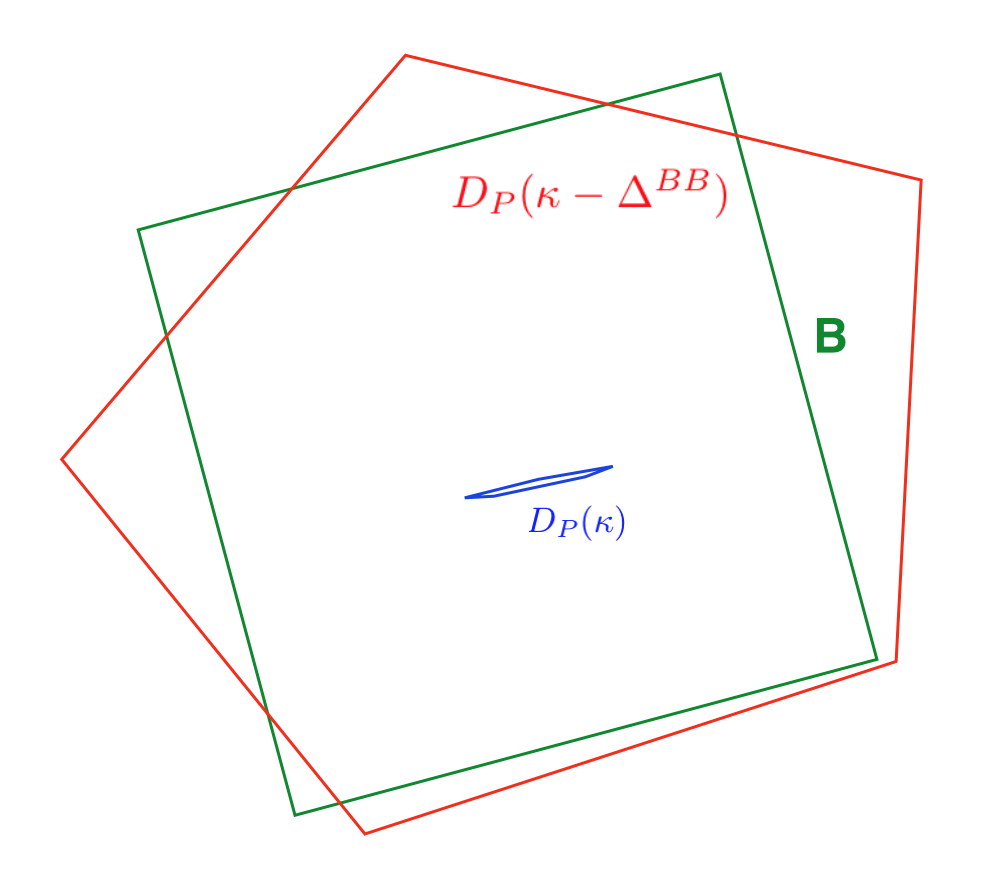
    We thus turn our attention to asserting that the fatness condition required for the kernel-approximation algorithm does indeed hold. In Section 6 we give a private (c,Δ)(c,\Delta)-approximation of the min bounding box problem — it returns a box that (a) contains DP​(κ)D_{P}(\kappa) and (b) with volume upper bounded by c⋅vol⁡(DP​(κ−Δ))c~\cdot~\mathrm{vol}(D_{P}(\kappa-\Delta)). Then, in Section 6.3 we argue that if vol⁡(DP​(κ))≥vol⁡(DP​(κ−Δ))/2\mathrm{vol}(D_{P}(\kappa))\geq\mathrm{vol}(D_{P}(\kappa-\Delta))/2 then this procedure also gives an affine transformation TT that makes 0​p​t​(T⁡(DP​(κ))CLOSE0pt(T(D_{P}(\kappa)) sufficiently large. (Obviously, if 𝒮\mathcal{S} is a (α,Δ)(\alpha,\Delta)-kernel for T​(DP​(κ))T(D_{P}(\kappa)) then T−1​(𝒮)T^{-1}(\mathcal{S}) is a (α,Δ)(\alpha,\Delta)-kernel for DP​(κ)D_{P}(\kappa).)

  • •

    In Section 7 we give a private algorithm for finding a “good” value of κ\kappa, one for which it does hold that vol⁡(DP​(κ))≥vol⁡(DP​(κ−Δ))/2\mathrm{vol}(D_{P}(\kappa))\geq\mathrm{vol}(D_{P}(\kappa-\Delta))/2. We formulate a certain query qq where any κ\kappa for which qP​(κ)q_{P}(\kappa) is large must also be a good κ\kappa, and then give a private algorithm for finding a κ\kappa with a large qP​(κ)q_{P}(\kappa)-value. The ε\varepsilon-differentially private algorithm we give is actually rather novel — it is based on a combination of the Exponential-Mechanism with additive Laplace noise. Its privacy is a result of arguing that for any neighboring PP and P′P^{\prime} where P′=P∪{x}P^{\prime}=P\cup\{x\} we can match κ\kappa with κ+1\kappa+1 so that |qP​(κ)−qP′​(κ+1)|≤1|q_{P}(\kappa)-q_{P^{\prime}}(\kappa+1)|\leq 1, and then using a few more observations that establish pure ε\varepsilon-differential privacy (rather than (ε,δ)(\varepsilon,\delta)-DP).

Our work thus culminates in the following theorem.

Theorem 2.

There exists an efficient (ε,δ)(\varepsilon,\delta)-differentially private algorithm, that for any sufficiently large dataset PP, where |P|≥Ω~​(d4​υ⋅Δ)|P|\geq\tilde{\Omega}(d^{4}\upsilon\cdot\Delta), with probability ≥1−β\geq 1-\beta finds a κ\kappa and a set 𝒮\mathcal{S} such that 𝒮\mathcal{S} is a (α,Δ)(\alpha,\Delta)-kernel of DP​(κ)D_{P}(\kappa) where Δ=O⁡(f⁡(d)ε⋅(1α)d2​log⁡(1δ)​log⁡(1α​β))\Delta=O(\frac{f(d)}{\varepsilon}\cdot(\frac{1}{\alpha})^{\frac{d}{2}}\sqrt{\log(\frac{1}{\delta})}\log(\frac{1}{\alpha\beta})) for some function f⁡(d)=2d2​polylog⁡(d)f(d)=2^{d^{2}\mathop{\mathrm{poly}}\log(d)}.

In fact, it is also required that Δ≥ΔBB​(d,υ,ε,δ,β)\Delta\geq\Delta^{\rm BB}(d,\upsilon,\varepsilon,\delta,\beta) where ΔBB\Delta^{\rm BB} is guarantee of the private min-bounding-box algorithm, as detailed in Theorem 27; yet this lower-bound holds under a very large regime of parameters. Moreover, there also exists a different algorithm that returns a somewhat better guarantee, replacing f⁡(d)f(d) with some f~​(d,υ)\tilde{f}(d,\upsilon)-function and reducing the dependency on α\alpha to (1/α)d−12(1/\alpha)^{\frac{d-1}{2}}, and more importantly — promising that 𝒮⊂DP​(κ−Δ)\mathcal{S}\subset D_{P}(\kappa-\Delta).

Additional Works.

In addition to the two works [BMNS19, KSS20] that privately find a point inside a convex hull, it is also worth mentioning the works regarding privately approximating the diameter [NSV16, NS18] (they return a O⁡(1)O(1)-approximation of the diameter that may miss a few points), and the work of [KMMS19] that privately approximates a kk-edges polygon yet requires a dataset of points where many lie inside the polygon and many lie outside the polygon. No additional works that we know of lie in the intersection of differential privacy and computational geometry. Computational geometry, of course, is a rich fied of computer science replete with many algorithms for numerous tasks in geometry. Our work only give private analogs to (a few of) the algorithms of [Cha02, AHV04], but there are far many more algorithms to be privatized and the reader is referred to [Hp11] for a survey of the field. Many works deal with computing the Tukey-depth and the Tukey region [RR98, LMM19], and others give statistical convergence rates for the Tukey-depth when the data is composed of i.i.d draws from a distribution [ZS00b, BF17, Bru19].

2 Preliminaries

2.1 Geometry

In this work we use ⟨⋅,⋅⟩\langle\cdot,\cdot\rangle to denote the inner-product between two vectors in ℝd\mathbb{R}^{d}. A closed half-space is defined by a vector uu and a scalar λ\lambda and it is the set {x∈ℝd:⟨x,u⟩≤λ}\{x\in\mathbb{R}^{d}:\langle x,u\rangle\leq\lambda\}. A polytope is the intersection of finitely many closed half-spaces. It is known that a polytope SS is a convex body: for any x,y∈Sx,y\in S and any λ∈[0,1]\lambda\in[0,1] it also holds that λ​x+(1−λ)​y∈S\lambda x+(1-\lambda)y\in S. Given a collection of points PP, their convex-hull is the set of all points that can be written as a convex combination of the points in PP. For a polytope PP and a point xx we define P−xP-x as the shift of PP by xx (namely z∈P−xz\in P-x iff ∃y∈P\exists y\in P s.t. z=y−xz=y-x), and we define by c​PcP the blow-up of PP by a scalar cc.

An inner product ⟨x,u⟩=‖x‖​‖u‖​cos⁡(∠⁡(x,u))\langle x,u\rangle=\|x\|\|u\|\cos(\angle(x,u)) is also known a projection of xx onto the subspace spanned by uu. A projection onto a subspace ΠV\Pi^{V} maps any x∈ℝdx\in\mathbb{R}^{d} to its closest point in the subspace VV. The following fact is well-known.

Fact 3.

Let SS be a convex body. Let uu be any vector and let Π⟂u\Pi^{\perp u} be the projection onto the subspace orthogonal to uu. Denote ℓ\ell as the max-length of the intersection of SS with any affine line in direction uu, and denote AA as the volume of the projection of SS onto the subspace orthogonal to uu, A=vol​(Π⟂u​(S))A=\mathrm{vol}(\Pi^{\perp u}(S)). Then A⋅ℓd≤vol⁡(S)≤A⋅ℓ\frac{A\cdot\ell}{d}\leq\mathrm{vol}(S)\leq A\cdot\ell.

The fact follows from reshaping SS so that it is contained in the “cylinder” whose base is AA and height is ℓ\ell, and contains a “pyramid” with base of AA and height of ℓ\ell.

The unit-sphere 𝕊d−1\mathbb{S}^{d-1} is the set of vectors in ℝd\mathbb{R}^{d} of length 11. The diameter of the convex body PP is defined as diam⁡(P)=maxp,q∈P⁡‖p−q‖\mathrm{diam}(P)=\max_{p,q\in P}\|p-q\|, and it is simple to see that diam⁡(P)=maxu∈𝕊d−1⁡maxp,q∈P​⟨p−q,u⟩\mathrm{diam}(P)=\max_{u\in\mathbb{S}^{d-1}}\max_{p,q\in P}\langle p-q,u\rangle. The width of a convex body PP is analogously defined as 0​p​t​(P)=minu∈𝕊d−1⁡maxp,q∈P​⟨p−q,u⟩0pt(P)=\min_{u\in\mathbb{S}^{d-1}}\max_{p,q\in P}\langle p-q,u\rangle. A ζ\zeta-angle cover of the unit sphere is a set of vectors VζV_{\zeta} such that for any v∈𝕊d−1v\in\mathbb{S}^{d-1} there exist uu such that ∠⁡(u,v)≤ζ\angle(u,v)\leq\zeta. It is known that each vector in the sphere can be characterized by d−1d-1 angles φ1,φ2,…,φd−1\varphi_{1},\varphi_{2},...,\varphi_{d-1} where φi∈[0,2​π]\varphi_{i}\in[0,2\pi] and for any other jj, φj∈[0,π]\varphi_{j}\in[0,\pi]. Therefore by discretizing the interval [0,π][0,\pi] we can create a ζ\zeta-angle cover of size 2​⌈π/ζ⌉d−12\lceil\pi/\zeta\rceil^{d-1}.

Proposition 4.

Let ζ<1/2\zeta<1/2. Let VζV_{\zeta} be a ζ\zeta-angle cover of 𝕊d−1\mathbb{S}^{d-1}. Then for any u∈𝕊d−1u\in\mathbb{S}^{d-1} the closest v∈Vζv\in V_{\zeta} satisfies that ‖u−v‖≤2​ζ\|u-v\|\leq\sqrt{2}\zeta.

Proof.

For a given uu and its closest vv we have that ‖u−v‖2=⟨u−v,u−v⟩=2⋅12−2⋅12​cos⁡(∠⁡(u,v))≤2−2​cos⁡(ζ)≤Taylor2−2​(1−ζ2)≤2​ζ2\|u-v\|^{2}=\langle u-v,u-v\rangle=2\cdot 1^{2}-2\cdot 1^{2}\cos(\angle(u,v))\leq 2-2\cos(\zeta)\stackrel{{\scriptstyle\rm Taylor}}{{\leq}}2-2(1-\zeta^{2})\leq 2\zeta^{2}. The fact that ζ<12\zeta<\frac{1}{2} allows us to lower bound the Taylor expansion of cos⁡(ζ)\cos(\zeta). ∎

Tukey Depth.

Given a finite set of points P⊂ℝdP\subset\mathbb{R}^{d}, the Tukey depth [TUK75] of a point x∈ℝdx\in\mathbb{R}^{d} w.r.t PP is defined TD⁡(x,P)=minu∈𝕊d−1⁡|{p∈P:⟨p,u⟩≤⟨x,u⟩}|\mathrm{TD}(x,P)=\min_{u\in\mathbb{S}^{d-1}}|\{p\in P:~\langle p,u\rangle\leq\langle x,u\rangle\}|. It is also the min-size of a set S⊂PS\subset P such that there exists a hyperplane separating xx from P∖SP\setminus S. Given PP and a depth parameter κ≥0\kappa\geq 0 we denote the κ\kappa-Tukey region as DP​(κ)={x∈ℝd:TD⁡(x,P)≥κ}D_{P}(\kappa)=\{x\in\mathbb{R}^{d}:\mathrm{TD}(x,P)\geq\kappa\}. Note that DP​(0)=ℝdD_{P}(0)=\mathbb{R}^{d} and DP​(1)=𝖢𝖧​(P)D_{P}(1)=\mathsf{CH}(P). It is known that for any set of points PP it holds that κ∗=maxx⁡TD⁡(x,P)\kappa^{*}=\max_{x}\mathrm{TD}(x,P) is upper bounded by |P|/2|P|/2 and lower bounded by |P|/(d+1)|P|/(d+1) (see [Ede87]). It is also known that for any κ\kappa, the set DP​(κ)D_{P}(\kappa) (assuming its non-empty) is a convex polytope which is the intersection of all closed halfspaces that contain at least n−κ+1n-\kappa+1 points out of PP [RR98], this yields a simple algorithm to compute the κ\kappa-Tukey region in time O⁡(n(d−1)​⌊d2⌋)O(n^{(d-1)\lfloor\frac{d}{2}\rfloor}). There is a faster algorithm to compute the κ\kappa-Tukey region in time O⁡(nd​log⁡n)O(n^{d}\log n) [LMM19], and so to compute all of the non-empty Tukey-regions in time O⁡(nd+1​log⁡n)O(n^{d+1}\log n). There is also an efficient algorithm [Liu17] for computing the Tukey-depth of a given point in time O⁡(nd−1​log⁡n)O(n^{d-1}\log n).

2.2 Differential Privacy

Differential privacy is a mathematically rigorous notion of preserving privacy in data analysis. Formally, two datasets PP and P′P^{\prime} are called neighboring if they differ on a single datum, and in thus work we assume that this means that |P​△​P′|=1|P\triangle P^{\prime}|=1.

Definition 5.

A randomized algorithm 𝒜{\cal A} is said to be (ε,δ)(\varepsilon,\delta)-differentially private (DP) if for any two neighboring datasets PP and P′P^{\prime} and for any set of possible outputs SS it holds that Pr[𝒜(P)∈S]≤eεPr[𝒜(P′)∈S]+δ\Pr[{\cal A}(P)\in S]\leq e^{\varepsilon}\Pr[{\cal A}(P^{\prime})\in S]+\delta. When δ=0\delta=0 we say 𝒜{\cal A} is ε\varepsilon-DP or ε\varepsilon-pure DP.

Differential privacy composes. Namely, if 𝒜{\cal A} is (ε,δ)(\varepsilon,\delta)-DP and ℬ{\cal B} is (ε′,δ′)(\varepsilon^{\prime},\delta^{\prime})-DP, then applying 𝒜{\cal A} and then applying ℬ{\cal B} sequentially on PP is a (ε+ε′,δ+δ′)(\varepsilon+\varepsilon^{\prime},\delta+\delta^{\prime})-DP algorithm (even when ℬ{\cal B} is chosen adaptively, based of 𝒜{\cal A}’s output). Moreover, post-processing the output of a (ε,δ)(\varepsilon,\delta)-DP algorithm cannot increase either ε\varepsilon or δ\delta. It is also worth noting the advanced-composition theorem of [DRV10], where the sequential application of kk (ε,δ)(\varepsilon,\delta)-DP algorithms yields in total an algorithm which is (ε​k​ln⁡(1/k​δ),2​k​δ)(\varepsilon\sqrt{k\ln(1/k\delta)},2k\delta)-DP (provided ε<1\varepsilon<1). Since we deal with a constant dimension dd, then whenever we compose poly(d)\mathop{\mathrm{poly}}(d)-many mechanisms, we rely on the basic composition; and whenever we compose exp⁡(d)\exp(d)-many mechanisms, we rely on the advanced composition.

Perhaps most common out of all DP-algorithms is the Laplace additive noise. Given a function ff that maps inputs to real numbers, we define its global sensitivity G​S​(f)=maxP,P′​neighbors⁡|f⁡(P)−f⁡(P′)|GS(f)=\max_{P,P^{\prime}{\rm neighbors}}|f(P)-f(P^{\prime})|. It is known that outputting f(P)+𝖫𝖺𝗉⁡(𝖦𝖲⁡(𝖿)/ε)f(P)+\mathop{\mathsf{Lap(GS(f)/\varepsilon)}} is ε\varepsilon-DP. Unfortunately, many of the functions we discuss in this work exhibit high global sensitivity, rendering this mechanism useless. It is also worth noting the Sparse Vector Technique which is a ε\varepsilon-DP algorithm that allows us to assess tt queries q1,q2,..,qtq_{1},q_{2},..,q_{t}, each with G​S​(qi)=1GS(q_{i})=1, and halt on the very first query that exceeds a certain (noisy) threshold. Our algorithms repeatedly rely on the SVT.

For more details on differential privacy the reader is deferred to the monographs [DR14, Vad17].

2.2.1 Private Approximation of Quasi-Concave Functions

In our work we use as “building blocks” several known techniques in differential privacy regarding private approximations of quasi-concave functions. We say a function q:ℝ→ℝq:\mathbb{R}\to\mathbb{R} is a quasi-concave function if for any x≤y≤zx\leq y\leq z it holds that

q⁡(y)≥min⁡{q⁡(x),q⁡(z)}q(y)\geq\min\{q(x),q(z)\}

Quasi-concave functions that obtain a maximum (namely, there exists some x∈ℝx\in\mathbb{R} such that q⁡(x)≥q⁡(y)q(x)\geq q(y) for any other y∈ℝy\in\mathbb{R}) have the property that the maximum is obtained on a single closed interval I=[x,y]I=[x,y] (we also consider the possibility of II containing only a single point, i.e., y=xy=x). Moreover, it follows that on the interval (−∞,x)(-\infty,x) the function qq is a monotone non-decreasing function and on the interval (y,∞)(y,\infty) the function qq is monotone non-increasing.

Perhaps more than any other application, approximating quasi-concave functions privately has been successfully applied in private learning of thresholds or quantiles, in a fairly large body of works [KLN+08, BNS13a, BNS13b, FX14, BNSV15, ALMM19, KLM+20]. Afterall, the function

q⁡(t)=−|n2−|{x∈P:x≤t}||q(t)=-\left|\frac{n}{2}-|\{x\in P:~x\leq t\}|\right|

is a quasi-concave function that allows one to approximate the median of a given dataset PP. We thus take the liberty to convert previous papers discussing private quantile-approximation to works that approximate privately any quasi concave function. We thus summarize the results in the following theorem.

Theorem 6.

Let qq be any function q:ℝ→ℝq:\mathbb{R}\to\mathbb{R} satisfying (i) qq is quasi-convace, (ii) qq has global-sensitivity 11 and (iii) for every closed interval II one can efficiently compute maxx∈I⁡q⁡(x)\max_{x\in I}q(x). Let 𝒢⊂ℝ\mathcal{G}\subset\mathbb{R} be a grid of granularity Υ=2−υ\Upsilon=2^{-\upsilon}, and denote q∗=maxx∈𝒢⁡q⁡(x)q^{*}=\max_{x\in\mathcal{G}}q(x). Then, for any 0<β<1/20<\beta<1/2 there exist differentially private algorithms that w.p. ≥1−β\geq 1-\beta return some x∈𝒢x\in\mathcal{G} such that q⁡(x)≥q∗−αqcq(x)\geq q^{*}-\alpha^{\rm qc} where

αqc​(ε,δ,β)={O⁡(υ+log⁡(1/β)ε),using ε-DP binary-searchO~​(log⁡(υ/β​ε​δ)ε),using the “Between Thresholds” Algorithm [BSU17]O⁡(8log∗⁡(υ)​log∗⁡(υ)ε⋅log⁡(log∗⁡(υ)β​δ))using the “RecConvace” algorithm [BNS13b]\alpha^{\rm qc}(\varepsilon,\delta,\beta)=\begin{cases}O(\frac{\upsilon+\log(1/\beta)}{\varepsilon}),&~\textrm{using $\varepsilon$-DP binary-search}\\ \tilde{O}(\frac{\log(\upsilon/\beta\varepsilon\delta)}{\varepsilon}),&~\textrm{using the ``Between Thresholds'' Algorithm~\cite[cite]{[\@@bibref{}{BunSU17}{}{}]}}\\ O\left(\frac{8^{\log^{*}(\upsilon)}\log^{*}(\upsilon)}{\varepsilon}\cdot\log(\frac{\log^{*}(\upsilon)}{\beta\delta})\right)&~\textrm{using the ``RecConvace'' algorithm~\cite[cite]{[\@@bibref{}{BeimelNS13b}{}{}]}}\\ \end{cases}

The first bound is given by standard ε\varepsilon-DP binary search algorithm (folklore). The second bound is given by the rather intuitive “Between Threshold” algorithm of Bun et al [BSU17] where instead of the standard counting function f⁡(z)=|{x∈P:x≤z}|f(z)=|\{x\in P:x\leq z\}| we use the function f(z)=maxx∈(−∞,z]q(x)−maxx∈[z,∞)q(x)f(z)=\max\limits_{x\in(-\infty,z]}q(x)-\max\limits_{x\in[z,\infty)}q(x) and set thresholds close to 00 (indicating a maximization point of qq). The third is from the RecConcave algorithm [BNS13b] that deals with approximating quasi-concave function, a rather intricate algorithm. We comment that it is unknown44 4 Uri Stemmer, private correspondence. whether the more recent work [KLM+20] that improves upon the bounds of RecConcave is applicable to general quasi-concave functions.

3 Tools, Part 1: The Tukey-Depth Completion Function

In this section we discuss the implementation of the following Tukey Depth Completion function. This function takes as a parameter a ii-long tuple of coordinates y¯\bar{y}, where 0≤i<d0\leq i<d, and scores each x∈ℝx\in\mathbb{R} with a value κ\kappa if the i+1i+1 prefix y¯∘x\bar{y}\circ x can be completed to a point with Tukey-depth of κ\kappa. Formally, we present the following definition(s).

Definition 7.

Fix d∈ℕd\in\mathbb{N} and let PP be a collection of points in ℝd\mathbb{R}^{d}. For any ii-tuple of coordinates y¯=(y1,y2,…,yi)\bar{y}=(y_{1},y_{2},...,y_{i}) where 0≤i≤d−10\leq i\leq d-1 we define the function 𝖳𝖣𝖢y¯:ℝ→ℝ\mathsf{TDC}_{\bar{y}}:\mathbb{R}\to\mathbb{R} by

𝖳𝖣𝖢y¯P(x)=max(z1,z2,…,zd−1−i)∈ℝd−i−1TD((y1,..,yi,x,z1,..,.zd−1−i),P)\mathsf{TDC}^{P}_{\bar{y}}(x)=\max_{(z_{1},z_{2},...,z_{d-1-i})\in\mathbb{R}^{d-i-1}}\mathrm{TD}\big((y_{1},..,y_{i},x,z_{1},..,.z_{d-1-i}),P\big) (1)

For any closed interval I=[a,b]⊂ℝI=[a,b]\subset\mathbb{R} we overload the definition of 𝖳𝖣𝖢\mathsf{TDC} to denote

𝖳𝖣𝖢y¯P​(I)=maxx∈[a,b]⁡𝖳𝖣𝖢y¯P​(x)\mathsf{TDC}^{P}_{\bar{y}}(I)=\max_{x\in[a,b]}\mathsf{TDC}^{P}_{\bar{y}}(x) (2)

note that for x∈ℝx\in\mathbb{R} it holds that 𝖳𝖣𝖢y¯P​(x)=𝖳𝖣𝖢y¯P​(I)\mathsf{TDC}^{P}_{\bar{y}}(x)=\mathsf{TDC}^{P}_{\bar{y}}(I) for the closed (degenerate) interval I=[x,x]I=[x,x].

Lastly, we introduce an additional variation that we will apply in our work. For any such y¯\bar{y} and any ℓ∈ℝ\ell\in\mathbb{R} we denote the following function.

ℓ−𝖳𝖣𝖢y¯P​(x)=min⁡{𝖳𝖣𝖢y¯P​(x),𝖳𝖣𝖢y¯P​(x+ℓ)}\ell\mathchar 45\relax\mathsf{TDC}_{\bar{y}}^{P}(x)=\min\{\mathsf{TDC}^{P}_{\bar{y}}(x),\mathsf{TDC}^{P}_{\bar{y}}(x+\ell)\} (3)

and similarly, use ℓ−𝖳𝖣𝖢y¯P​(I)=maxx∈I⁡ℓ−𝖳𝖣𝖢y¯P​(x)\ell\mathchar 45\relax\mathsf{TDC}_{\bar{y}}^{P}(I)=\max\limits_{x\in I}\ell\mathchar 45\relax\mathsf{TDC}_{\bar{y}}^{P}(x). We omit the superscript PP whenever the dataset is clear.

It is worth noting that the definition of the 𝖳𝖣𝖢\mathsf{TDC}-function is w.r.t. the real Euclidean space and not just points on a grid. Later we discuss the refinement of the grid required for finding a point whose 𝖳𝖣𝖢\mathsf{TDC} w.r.t. the grid 𝒢d\mathcal{G}^{d} is equal.

We begin with a simple property of the 𝖳𝖣𝖢\mathsf{TDC} function, we show that the 𝖳𝖣𝖢\mathsf{TDC}-function, as well as the ℓ−𝖳𝖣𝖢\ell\mathchar 45\relax\mathsf{TDC}-function, are both quasi-concave functions. (The first part of the claim was proven in [BMNS19].)

Proposition 8.

Fix ii and fix an ii-tuple y¯\bar{y}. For any a≤b≤ca\leq b\leq c on the grid we have that

𝖳𝖣𝖢y¯​(b)≥min⁡{𝖳𝖣𝖢y¯​(a),𝖳𝖣𝖢y¯​(c)}\mathsf{TDC}_{\bar{y}}(b)\geq\min\left\{\mathsf{TDC}_{\bar{y}}(a),\mathsf{TDC}_{\bar{y}}(c)\right\}

In addition for any ℓ>0\ell>0 we also have that

ℓ−𝖳𝖣𝖢y¯​(b)≥min⁡{ℓ−𝖳𝖣𝖢y¯​(a),ℓ−𝖳𝖣𝖢y¯​(c)}\ell\mathchar 45\relax\mathsf{TDC}_{\bar{y}}(b)\geq\min\left\{\ell\mathchar 45\relax\mathsf{TDC}_{\bar{y}}(a),\ell\mathchar 45\relax\mathsf{TDC}_{\bar{y}}(c)\right\}
Proof.

If b=ab=a or b=cb=c then the claim trivially holds. Assuming a<b<ca<b<c, denote b=λ​a+(1−λ)​cb=\lambda a+(1-\lambda)c for the suitable scalar λ∈(0,1)\lambda\in(0,1). Denote κ=min⁡{𝖳𝖣𝖢y¯​(a),𝖳𝖣𝖢y¯​(c)}\kappa=\min\{\mathsf{TDC}_{\bar{y}}(a),\mathsf{TDC}_{\bar{y}}(c)\}. Let z¯a\bar{z}_{a} and z¯c\bar{z}_{c} be the two completions such that TD⁡(y¯∘a∘z¯a),TD⁡(y¯∘c∘z¯c)≥κ\mathrm{TD}\Big(\bar{y}\circ a\circ\bar{z}_{a}\Big),\mathrm{TD}\Big(\bar{y}\circ c\circ\bar{z}_{c}\Big)\geq\kappa. It follows that the two points pa=(y¯∘a∘z¯a)p_{a}=\Big(\bar{y}\circ a\circ\bar{z}_{a}\Big) and pc=(y¯∘c∘z¯c)p_{c}=\Big(\bar{y}\circ c\circ\bar{z}_{c}\Big) are in DP​(κ)D_{P}(\kappa). Due to the convexity of DP​(κ)D_{P}(\kappa) it holds that the point pb=λ​pa+(1−λ)​pcp_{b}=\lambda p_{a}+(1-\lambda)p_{c} also belongs to DP​(κ)D_{P}(\kappa). Since the i+1i+1 coordinate of pbp_{b} is bb it follows that 𝖳𝖣𝖢y¯​(b)≥κ\mathsf{TDC}_{\bar{y}}(b)\geq\kappa.

As for the function ℓ−𝖳𝖣𝖢y¯\ell\mathchar 45\relax\mathsf{TDC}_{\bar{y}}, note that by definition

min⁡{ℓ−𝖳𝖣𝖢y¯​(a),ℓ−𝖳𝖣𝖢y¯​(c)}=min⁡{𝖳𝖣𝖢y¯​(a),𝖳𝖣𝖢y¯​(c),𝖳𝖣𝖢y¯​(a+ℓ),𝖳𝖣𝖢y¯​(c+ℓ)}=defρ\min\left\{\ell\mathchar 45\relax\mathsf{TDC}_{\bar{y}}(a),\ell\mathchar 45\relax\mathsf{TDC}_{\bar{y}}(c)\right\}=\min\{\mathsf{TDC}_{\bar{y}}(a),\mathsf{TDC}_{\bar{y}}(c),\mathsf{TDC}_{\bar{y}}(a+\ell),\mathsf{TDC}_{\bar{y}}(c+\ell)\}\stackrel{{\scriptstyle\rm def}}{{=}}\rho

And since we have shown the quasi-concavity of 𝖳𝖣𝖢\mathsf{TDC} then we have that

𝖳𝖣𝖢y¯​(b)\displaystyle\mathsf{TDC}_{\bar{y}}(b) ≥min⁡{𝖳𝖣𝖢y¯​(a),𝖳𝖣𝖢y¯​(c)}≥ρ\displaystyle\geq\min\{\mathsf{TDC}_{\bar{y}}(a),\mathsf{TDC}_{\bar{y}}(c)\}\geq\rho
and similarly that
𝖳𝖣𝖢y¯​(b+ℓ)\displaystyle\mathsf{TDC}_{\bar{y}}(b+\ell) ≥min⁡{𝖳𝖣𝖢y¯​(a+ℓ),𝖳𝖣𝖢y¯​(c+ℓ)}≥ρ\displaystyle\geq\min\{\mathsf{TDC}_{\bar{y}}(a+\ell),\mathsf{TDC}_{\bar{y}}(c+\ell)\}\geq\rho
so it holds that
ℓ−𝖳𝖣𝖢y¯​(b)\displaystyle\ell\mathchar 45\relax\mathsf{TDC}_{\bar{y}}(b) =min⁡{𝖳𝖣𝖢y¯​(b),𝖳𝖣𝖢y¯​(b+ℓ)}≥ρ=min⁡{ℓ−𝖳𝖣𝖢y¯​(a),ℓ−𝖳𝖣𝖢y¯​(c)}\displaystyle=\min\{\mathsf{TDC}_{\bar{y}}(b),\mathsf{TDC}_{\bar{y}}(b+\ell)\}\geq\rho=\min\left\{\ell\mathchar 45\relax\mathsf{TDC}_{\bar{y}}(a),\ell\mathchar 45\relax\mathsf{TDC}_{\bar{y}}(c)\right\}

∎

Having established the quasi-concavity of 𝖳𝖣𝖢y¯\mathsf{TDC}_{\bar{y}} it follows that on the real line the values of the function ascend from 00 to the max-value, then descend back to 00. In particular, for any (integer) κ\kappa from 00 to the max-value of the 𝖳𝖣𝖢y¯\mathsf{TDC}_{\bar{y}}-function, there exists an interval [aκ,bκ][a_{\kappa},b_{\kappa}] such that for any x∈[aκ,bκ]x\in[a_{\kappa},b_{\kappa}] it holds that 𝖳𝖣𝖢y¯​(x)≥κ\mathsf{TDC}_{\bar{y}}(x)\geq\kappa. And so, we give an algorithm that finds these sets of nested intervals {[aκ,bκ]}κ>0\{[a_{\kappa},b_{\kappa}]\}_{\kappa>0}, and then finds the maximum κ\kappa whose interval intersect the given point xx or interval II.

Algorithm 1 Pre-processing for Computing the 𝖳𝖣𝖢\mathsf{TDC}-function

Input: P⊂ℝdP\subset\mathbb{R}^{d}; an ii-tuple y¯=(y1,y2,..,yi)\bar{y}=(y_{1},y_{2},..,y_{i}).
Output: A collection of nested intervals.

1:  for each κ\kappa from 11 to n2\frac{n}{2} do
2:   Compute the κ\kappa-Tukey region DP​(κ)D_{P}(\kappa).
3:   Compute the intersection DP​(κ)∩Sy¯D_{P}(\kappa)\cap S_{\bar{y}} where Sy¯S_{\bar{y}} is the affine subspace Sy¯={y¯∘x¯:x¯∈ℝd−i}S_{\bar{y}}=\{\bar{y}\circ\bar{x}:~\bar{x}\in\mathbb{R}^{d-i}\}.
4:   if (DP​(κ)∩Sy¯=∅D_{P}(\kappa)\cap S_{\bar{y}}=\emptyset) then break for-loop
5:   Compute aκa_{\kappa} and bκb_{\kappa} where aκ\displaystyle a_{\kappa} =min⁡⟨e¯i+1,y¯∘x¯⟩\displaystyle=\min\langle\bar{e}_{i+1},\bar{y}\circ\bar{x}\rangle s.t. x¯∈DP​(κ)∩Sy¯\displaystyle\bar{x}\in D_{P}(\kappa)\cap S_{\bar{y}}  and  bκ\displaystyle b_{\kappa} =max⁡⟨e¯i+1,y¯∘x¯⟩\displaystyle=\max\langle\bar{e}_{i+1},\bar{y}\circ\bar{x}\rangle s.t. x¯∈DP​(κ)∩Sy¯\displaystyle\bar{x}\in D_{P}(\kappa)\cap S_{\bar{y}}
6:  end for
7:  return the collection {[aκ,bκ]}\{[a_{\kappa},b_{\kappa}]\}
Theorem 9.

For any 0≤i<d0\leq i<d and any ii-tuple y¯\bar{y}, Algorithm 1 runs in time polynomial in nn and υ\upsilon and exponential in dd and returns a collection of nested intervals such that for any interval I⊂ℝI\subset\mathbb{R} it holds that 𝖳𝖣𝖢y¯​(I)=max⁡{κ:I∩[aκ,bκ]≠∅}\mathsf{TDC}_{\bar{y}}(I)=\max\{\kappa:I\cap[a_{\kappa},b_{\kappa}]\neq\emptyset\}.

Proof.

Since there are at most n/2n/2 possible intervals returned by the algorithm and each is formed by solving a LP in npoly⁡(d)n^{{\rm poly}(d)} constraints, the claim regarding the runtime of the algorithm holds. In fact, it is known that the exact computation of the Tukey region takes T⁡(n,d)=O⁡(n(d−1)​⌊d/2⌋)T(n,d)=O(n^{(d-1)\lfloor d/2\rfloor}) time, a computation that returns a set of ≤T⁡(n,d)\leq T(n,d) vetrices that form the boundary of the DP​(κ)D_{P}(\kappa)-polytope. Thus, solving each LP involves d−id-i variables with T⁡(n,d)T(n,d) many constraints, so it takes at most O⁡((d−i)!​T​(n,d))O((d-i)!T(n,d))-time [Sei91].

Secondly, each DP​(κ)D_{P}(\kappa) is a convex polytope so its intersection with the (convex) affine subspace Sy¯S_{\bar{y}} is also a convex polytope. Now, since for any κ<κ′\kappa<\kappa^{\prime} we have that DP​(κ′)⊂DP​(κ)D_{P}(\kappa^{\prime})\subset D_{P}(\kappa) then — denoting x¯κ′\bar{x}_{\kappa^{\prime}} as the vector that obtains aκ′a_{\kappa^{\prime}} — we have that x¯κ′\bar{x}_{\kappa^{\prime}} is a valid solution for the minimization LP for DP​(κ)D_{P}(\kappa) hence aκ≤⟨e¯i+1,y¯∘x¯κ′⟩=aκ′a_{\kappa}\leq\langle\bar{e}_{i+1},\bar{y}\circ\bar{x}_{\kappa^{\prime}}\rangle=a_{\kappa^{\prime}}, and similarly, bκ≥bκ′b_{\kappa}\geq b_{\kappa^{\prime}}; thus [aκ′,bκ′]⊂[aκ,bκ][a_{\kappa^{\prime}},b_{\kappa^{\prime}}]\subset[a_{\kappa},b_{\kappa}]. This implies the set of intervals are nested in one another.

Next fix any interval I⊂ℝI\subset\mathbb{R}. We argue that for any κ\kappa such that there exists some x∈Ix\in I that also falls inside the interval [aκ,bκ][a_{\kappa},b_{\kappa}], we have that 𝖳𝖣𝖢y¯​(x)≥κ\mathsf{TDC}_{\bar{y}}(x)\geq\kappa, making 𝖳𝖣𝖢y¯​(I)≥κ\mathsf{TDC}_{\bar{y}}(I)\geq\kappa. The reason is the following: denote the vectors u¯=(y¯∘aκ∘z¯)\bar{u}=\big(\bar{y}\circ a_{\kappa}\circ\bar{z}\big) and v¯=(y¯∘bκ∘z¯′)\bar{v}=\big(\bar{y}\circ b_{\kappa}\circ\bar{z}^{\prime}\big) as two vectors in DP​(κ)∩Sy¯D_{P}(\kappa)\cap S_{\bar{y}} that obtain aκa_{\kappa} and bκb_{\kappa}. These vectors give that 𝖳𝖣𝖢y¯​(aκ)≥κ\mathsf{TDC}_{\bar{y}}(a_{\kappa})\geq\kappa and 𝖳𝖣𝖢y¯​(bκ)≥κ\mathsf{TDC}_{\bar{y}}(b_{\kappa})\geq\kappa so by quasi-concaveness we have that 𝖳𝖣𝖢y¯​(x)≥k\mathsf{TDC}_{\bar{y}}(x)\geq k. This shows that 𝖳𝖣𝖢y¯​(I)≥max⁡{κ:I∩[aκ,bκ]≠∅}\mathsf{TDC}_{\bar{y}}(I)\geq\max\{\kappa:I\cap[a_{\kappa},b_{\kappa}]\neq\emptyset\}. Conversely, denote κ∗=𝖳𝖣𝖢y¯​(I)\kappa^{*}=\mathsf{TDC}_{\bar{y}}(I), then for some x∈Ix\in I we have that 𝖳𝖣𝖢y¯​(x)=κ∗\mathsf{TDC}_{\bar{y}}(x)=\kappa^{*} which means that for some completion u¯=(y¯∘x∘z¯)∈DP​(κ∗)∩Sy¯\bar{u}=\big(\bar{y}\circ x\circ\bar{z}\big)\in D_{P}(\kappa^{*})\cap S_{\bar{y}}, and so we have that aκ∗≤x≤bκ∗a_{\kappa^{*}}\leq x\leq b_{\kappa^{*}} as aκ∗a_{\kappa^{*}} (resp. bκ∗b_{\kappa^{*}}) is a solution for a minimization (resp. maximization) problem over a domain containing u¯\bar{u}. Thus I∩[aκ∗,bκ∗]≠∅I\cap[a_{\kappa^{*}},b_{\kappa^{*}}]\neq\emptyset making κ∗≤max⁡{κ:I∩[aκ,bκ]≠∅}\kappa^{*}\leq\max\{\kappa:I\cap[a_{\kappa},b_{\kappa}]\neq\emptyset\}. ∎

Now, given the collection of intervals returned by Algorithm 1, which is in essence a set of ≤2​κ∗≤n\leq 2\kappa^{*}\leq n points

a1≤a2≤…≤aκ∗≤bκ∗≤bκ∗−1≤…≤b2≤b1a_{1}\leq a_{2}\leq...\leq a_{\kappa^{*}}\leq b_{\kappa^{*}}\leq b_{\kappa^{*}-1}\leq...\leq b_{2}\leq b_{1} (4)

on the real line where the 𝖳𝖣𝖢y¯\mathsf{TDC}_{\bar{y}}-function changes its value, we argue that for any interval II computing 𝖳𝖣𝖢y¯​(I)\mathsf{TDC}_{\bar{y}}(I) is simple and can be done in O⁡(log⁡(κ∗))=O⁡(log⁡(n))O(\log(\kappa^{*}))=O(\log(n))-time by the following scheme. Denoting I=[p,q]I=[p,q] we have:

  • •

    If q<aκ∗q<a_{\kappa^{*}} then II is contained in the part of the real line where 𝖳𝖣𝖢y¯\mathsf{TDC}_{\bar{y}} is monotone non-decreasing, thus 𝖳𝖣𝖢y¯​(I)=𝖳𝖣𝖢y¯​(q)\mathsf{TDC}_{\bar{y}}(I)=\mathsf{TDC}_{\bar{y}}(q), so using binary search we find κ\kappa such that aκ−1<q≤aκa_{\kappa-1}<q\leq a_{\kappa} and return it.

  • •

    Symmetrically, if p>bκ∗p>b_{\kappa^{*}} then II is contained in the part of the real line where 𝖳𝖣𝖢y¯\mathsf{TDC}_{\bar{y}} is monotone non-increasing, thus 𝖳𝖣𝖢y¯​(I)=𝖳𝖣𝖢y¯​(p)\mathsf{TDC}_{\bar{y}}(I)=\mathsf{TDC}_{\bar{y}}(p), so using binary search we find κ\kappa such that bκ≥p>bκ−1b_{\kappa}\geq p>b_{\kappa-1} and return it.

  • •

    Otherwise, q≥aκ∗q\geq a_{\kappa^{*}} and p≤bκ∗p\leq b_{\kappa^{*}} which means I∩[aκ∗,bκ∗]≠∅I\cap[a_{\kappa^{*}},b_{\kappa^{*}}]\neq\emptyset and so we return κ∗\kappa^{*}.

Next, in order to compute ℓ−𝖳𝖣𝖢y¯​(x)\ell\mathchar 45\relax\mathsf{TDC}_{\bar{y}}(x) we just compute 𝖳𝖣𝖢y¯​(x),𝖳𝖣𝖢y¯​(x+ℓ)\mathsf{TDC}_{\bar{y}}(x),\mathsf{TDC}_{\bar{y}}(x+\ell) and take the min of the two values, so this takes O⁡(log⁡(n))O(\log(n)) time as well.

Lastly, in order to compute ℓ−𝖳𝖣𝖢y¯​(I)\ell\mathchar 45\relax\mathsf{TDC}_{\bar{y}}(I), we append the collection of 2​κ∗2\kappa^{*} change-points with the set {aκ+ℓ:1≤κ≤k∗}∪{bκ−ℓ:1≤κ≤k∗}\{a_{\kappa}+\ell:~1\leq\kappa\leq k^{*}\}\cup\{b_{\kappa}-\ell:~1\leq\kappa\leq k^{*}\} and sort the 4​κ∗4\kappa^{*} points. This is a superset of all the change points of ℓ−𝖳𝖣𝖢y¯\ell\mathchar 45\relax\mathsf{TDC}_{\bar{y}}: it is clear that between any pair of consecutive points (a′,b′)(a^{\prime},b^{\prime}) the function ℓ−𝖳𝖣𝖢y¯\ell\mathchar 45\relax\mathsf{TDC}_{\bar{y}} takes the same value (because both (a′,b′)(a^{\prime},b^{\prime}) and (a′+ℓ,b′+ℓ)(a^{\prime}+\ell,b^{\prime}+\ell) are contained in a pair consecutive points among the original points in Eq (4)). We then compute the value of ℓ−𝖳𝖣𝖢y¯\ell\mathchar 45\relax\mathsf{TDC}_{\bar{y}} on each interval using a representative x∈(a′,b′)x\in(a^{\prime},b^{\prime}) and omit from the 4​κ∗4\kappa^{*} any point in which the value of ℓ−𝖳𝖣𝖢y¯\ell\mathchar 45\relax\mathsf{TDC}_{\bar{y}} doesn’t change. As κ∗≤n/2\kappa^{*}\leq n/2 then this takes O⁡(n​log⁡(n))O(n\log(n)). Once we have a sorted list of points on the real line where the value of ℓ−𝖳𝖣𝖢y¯\ell\mathchar 45\relax\mathsf{TDC}_{\bar{y}}-function change, we can now compute the value of the quasi-concave function ℓ−𝖳𝖣𝖢y¯​(I)\ell\mathchar 45\relax\mathsf{TDC}_{\bar{y}}(I) in a similar fashion to computing 𝖳𝖣𝖢y¯\mathsf{TDC}_{\bar{y}} in O⁡(log⁡(n))O(\log(n))-time.

Extension.

We comment that the above-algorithm works for any set of convex polytopes C1⊃C2⊃C3⊃..C_{1}\supset C_{2}\supset C_{3}\supset.. with at most npoly(d)n^{\mathop{\mathrm{poly}}(d)}-vertices each. We will rely on the this fact later, when we work with projections of the various Tukey-regions. However, one of the key uses to the 𝖳𝖣𝖢\mathsf{TDC}-function we rely on is when we rotate directions so that the first axis aligns with a given direction vv. In such a case, this is equivalent to rotating the set PP, so we use the notation 𝖳𝖣𝖢y¯Rv​(P)\mathsf{TDC}_{\bar{y}}^{R_{v}(P)} and on occasion just 𝖳𝖣𝖢y¯Rv\mathsf{TDC}_{\bar{y}}^{R_{v}}.

Grid Refinement.

This establishes that for any 0≤i≤d−10\leq i\leq d-1 and any y¯\bar{y} there exists an efficient (with pre-processing time of O⁡(d!​nd⁡(d−1)/2)O(d!n^{d(d-1)/2}) and query time of O⁡(log⁡(n))O(\log(n))) algorithm that computes 𝖳𝖣𝖢y¯​(x)\mathsf{TDC}_{\bar{y}}(x) and ℓ−𝖳𝖣𝖢y¯​(x)\ell\mathchar 45\relax\mathsf{TDC}_{\bar{y}}(x). But as Beimel et al [BMNS19] noted, it is not a-priori clear that the coordinates of the completion lie on the same grid 𝒢d\mathcal{G}^{d} we start with.

To this we provide two answers. The first, which we prefer by far, is that we can keep using the same grid 𝒢\mathcal{G}, and each time we find a point pp we instead of formally stating “we find a point pp inside the convex body” we use “we find a point pp within distance d​Υ\sqrt{d}\Upsilon from a point inside the convex body.” After all, our work already deals with approximations, so under the (rather benign) premise that the diameter of the convex body is sufficiently larger than Υ\Upsilon, this little additive factor changes very little in the overall scheme.

The second answer is to use a refinement of the grid 𝒢\mathcal{G} into some 𝒢′\mathcal{G}^{\prime}. This approach is described here, in order for our results to be comparable with the results of [BMNS19, KSS20] regarding finding a point inside the convex-hull. However, past this section we assume this refinement has already happened as a pre-processing step for our analysis and so we set 𝒢←𝒢′\mathcal{G}\leftarrow\mathcal{G}^{\prime} and continue with the remainder of the algorithms as is.

In order to construct the grid 𝒢′\mathcal{G}^{\prime}, we begin with the observation of Kaplan et al [KSS20] that for any κ\kappa, the vertices of DP​(κ)D_{P}(\kappa) lie on a grid 𝒢~d\tilde{\mathcal{G}}^{d} with granularity of Υ~=d−d⁡(d+1)2​Υd2\tilde{\Upsilon}=d^{\frac{-d(d+1)}{2}}\Upsilon^{d^{2}}. We also use the notation ξ=1/Υ~\xi=1/\tilde{\Upsilon}. We argue inductively that when applying 𝖳𝖣𝖢\mathsf{TDC}-sequentially to reveal the coordinates of a point inside the convex hull, we obtain a point pp whose iith coordinate lies on a grid of granularity lower bounded by ∏j=1i(Υ~/j)j\prod_{j=1}^{i}(\tilde{\Upsilon}/\sqrt{j})^{j}. Note, this makes our grid (much like the grid in [BMNS19]) highly unbalanced: on the first axis it suffices to use a discretization of Υ~\tilde{\Upsilon}, but on the dd-th axis we require a discretization of (Υ~/d)O⁡(d2)(\tilde{\Upsilon}/\sqrt{d})^{O(d^{2})}.

The claim is proven inductively. Let {aκi,bκi}κ=1κ∗\{a_{\kappa}^{i},b_{\kappa}^{i}\}_{\kappa=1}^{\kappa^{*}} be the collection of coordinates returned by Algorithm 1 in the process of computing 𝖳𝖣𝖢y¯​(x)\mathsf{TDC}_{\bar{y}}(x) where for each ii the prefix y¯\bar{y} is precisely the first ii coordinates of pp. Now, for i=1i=1 it is clear that each aκ1a_{\kappa}^{1} or bκ1b_{\kappa}^{1} is a coordinate of some vertex of DP​(κ)D_{P}(\kappa) and so it has granularity Υ~\tilde{\Upsilon}. Thus it suffices to place the grid 𝒢~\tilde{\mathcal{G}} on the [0,1][0,1]-interval find use a DP-algorithm that returns a point on this grid, and so the first coordinate p1p_{1} has granularity Υ~\tilde{\Upsilon}. Now, for each i+1i+1, the coordinates aκi+1,bκi+1a_{\kappa}^{i+1},b_{\kappa}^{i+1} are the i+1i+1-coordinates of two vertices of DP(κ)∩S(p1,..,pi)D_{P}(\kappa)\cap S_{(p_{1},..,p_{i})}. For brevity we denote p¯=(p1,..,pi)\bar{p}=(p_{1},..,p_{i}). Such a vertex is found when we take a (i+1)(i+1)-facet of DP​(κ)D_{P}(\kappa), whose vertices we denote as v1,v2,…,vi+1v^{1},v^{2},...,v^{i+1}, and find the intersection of Sp¯S_{\bar{p}} with this facet. So we check if there exists a point in this facet whose first ii coordinates are p¯\bar{p} and if so, retrieve its i+1i+1-coordinate. Namely, we see if p¯\bar{p} is a convex combination of the i+1i+1 vectors which are the ii-prefixes of the facet’s vertices, denoted as v¯1,…,v¯i+1\bar{v}^{1},...,\bar{v}^{i+1}; if indeed for some convex combination p¯=∑j=1i+1λj​v¯j\bar{p}=\sum_{j=1}^{i+1}\lambda_{j}\bar{v}^{j} then the i+1i+1-coordinate is ∑j=1i+1λj​vi+1j\sum_{j=1}^{i+1}\lambda_{j}v^{j}_{i+1}. Finding this convex combination requires that we solve a system of i+1i+1 linear constraints M​λ¯=(p¯,1)M\bar{\lambda}=(\bar{p},1) where each column of MM is composed of the ii-dimensional vector v¯j\bar{v}^{j} concatenated with 11, and the RHS is composed of p¯\bar{p} concatenated with 11. Thus λ¯=M−1​(p¯,1)\bar{\lambda}=M^{-1}(\bar{p},1), and the i+1i+1 coordinate we are after is a dot-product of M−1​(p¯,1)M^{-1}(\bar{p},1) with the vector u¯=(vi+11,vi+22,…,vi+1i+1)\bar{u}=(v^{1}_{i+1},v^{2}_{i+2},...,v^{i+1}_{i+1}) whose coordinates lies on 𝒢~\tilde{\mathcal{G}}.

Note that MM is composed of coordinates that lie on 𝒢~\tilde{\mathcal{G}} as it is composed of prefixes of vertices of DP​(κ)D_{P}(\kappa) and ones. Thus each coordinate of MM has granularity Υ~\tilde{\Upsilon}, and so ξ​M\xi M is an integer matrix with entries in [0,ξ][0,\xi]. By Hadamard’s inequality, det(ξ​M)≤(i+1​ξ)i+1\det(\xi M)\leq(\sqrt{i+1}\xi)^{i+1}, and so, writing (ξ​M)−1(\xi M)^{-1} using the adjugate formula, each entry of (ξ​M)−1(\xi M)^{-1} can be written as a fraction with a denominator of not larger than (i+1​ξ)i+1(\sqrt{i+1}\xi)^{i+1}. By our induction hypothesis, each coordinate of (p1,..,pi)(p_{1},..,p_{i}) can be written as a rational fraction with the same denominator, and the denominator doesn’t exceed ∏j=1i(j​ξ)j\prod_{j=1}^{i}(\sqrt{j}\xi)^{j}. Lastly, by definition each coordinate of u¯\bar{u} can be written as a fraction with denominator ξ\xi, so ξ​u¯\xi\bar{u} is a vector of integers. This means that ⟨M−1​(p¯,1),u¯⟩=⟨ξ⋅(ξ​M)−1​(p,1),u¯⟩=⟨(ξ​M)−1​(p¯,1),ξ​u¯⟩\langle M^{-1}(\bar{p},1),\bar{u}\rangle=\langle\xi\cdot(\xi M)^{-1}(p,1),\bar{u}\rangle=\langle(\xi M)^{-1}(\bar{p},1),\xi\bar{u}\rangle can be written as a rational fraction where its denominator doesn’t exceed ∏j=1i+1(j​ξ)j\prod_{j=1}^{i+1}(\sqrt{j}\xi)^{j}.

This proves that the level of discretization we require for any axis is bounded below by d−(d+1)​(d+2)4⋅Υ~−(d+1)​(d+2)2=d−O⁡(d4)​Υd4+3​d3+2​d22≥Υ4​d4d^{-\frac{(d+1)(d+2)}{4}}\cdot\tilde{\Upsilon}^{-\frac{(d+1)(d+2)}{2}}=d^{-O(d^{4})}\Upsilon^{\frac{d^{4}+3d^{3}+2d^{2}}{2}}\geq\Upsilon^{4d^{4}} (assuming d−1>Υd^{-1}>\Upsilon).

Summary.

Now that we refined the grid from 𝒢\mathcal{G} to 𝒢′\mathcal{G}^{\prime} with granularity Υ4​d4=2−υ⁡(4​d4)\Upsilon^{4d^{4}}=2^{-\upsilon(4d^{4})}, we can apply any DP-algorithm that w.p.≥1−β\geq 1-\beta returns a point on 𝒢′\mathcal{G}^{\prime} with roughly the same value of the maximal value. This gives a DP-algorithm that returns w.p.≥1−β\geq 1-\beta a point x∈𝒢′x\in\mathcal{G}^{\prime} with either 𝖳𝖣𝖢y¯\mathsf{TDC}_{\bar{y}}-value or ℓ−𝖳𝖣𝖢y¯\ell\mathchar 45\relax\mathsf{TDC}_{\bar{y}}-value which is αqc​(⋅,⋅,⋅)\alpha^{\rm qc}(\cdot,\cdot,\cdot)-close to the max-possible value on the grid. Altogether, we have the following corollary.55 5 Note that we have not bothered applying the advanced composition theorem [DRV10] since we assume dd is a small constant.

Corollary 10.

Fix ε>0\varepsilon>0, δ≥0\delta\geq 0, β∈(0,1/2)\beta\in(0,1/2). There exists an efficient (ε,δ)(\varepsilon,\delta)-DP-algorithm, denoted DPPointInTukeyRegion, that takes as input a dataset PP and a parameter κ\kappa where DP​(κ)≠∅D_{P}(\kappa)\neq\emptyset and w.p. ≥1−β\geq 1-\beta returns a point x¯∈(𝒢′)d\bar{x}\in(\mathcal{G}^{\prime})^{d} whose Tukey-depth is at least

κ−d​αqc​(εd,δd,βd)≥nd+1−d​αqc​(εd,δd,βd)\kappa-d\alpha^{\rm qc}(\frac{\varepsilon}{d},\frac{\delta}{d},\frac{\beta}{d})\geq\frac{n}{d+1}-d\alpha^{\rm qc}(\frac{\varepsilon}{d},\frac{\delta}{d},\frac{\beta}{d}) (5)

In particular, for any κ≥0\kappa\geq 0 we return a point of Tukey-depth ≥κ\geq\kappa provided n=Ω⁡(d​κ+d2​αqc​(εd,δd,βd))n=\Omega(d\kappa+d^{2}\alpha^{\rm qc}(\frac{\varepsilon}{d},\frac{\delta}{d},\frac{\beta}{d}))

={Ω⁡(d​κ+d3​d4​υ+log⁡(d/β)ε),Using the ε-DP binary-searchΩ~​(d​κ+d3​log⁡(d​υ/β​ε​δ)ε),Using the “Between Thresholds” algorithmΩ⁡(d​κ+d3​8log∗⁡(d​υ)​log∗⁡(d​υ)⋅log⁡(d​log∗⁡(υ)/δ​β)ε),Using the “RecConcave” algorithm=\begin{cases}\Omega(d\kappa+d^{3}\frac{d^{4}\upsilon+\log(d/\beta)}{\varepsilon}),&~\textrm{Using the $\varepsilon$-DP binary-search}\\ \tilde{\Omega}(d\kappa+d^{3}\frac{\log(d\upsilon/\beta\varepsilon\delta)}{\varepsilon}),&~\textrm{Using the ``Between Thresholds'' algorithm}\\ \Omega(d\kappa+d^{3}\frac{8^{\log^{*}(d\upsilon)}\log^{*}(d\upsilon)\cdot\log(d\log^{*}(\upsilon)/\delta\beta)}{\varepsilon}),&~\textrm{Using the ``RecConcave'' algorithm}\\ \end{cases} (6)

Again, we comment that quantitatively, the results are just as those obtained by [BMNS19]. The key improvement of our work is the runtime which decreases from poly(1/Υ)\mathop{\mathrm{poly}}(1/\Upsilon) to poly(υ)\mathop{\mathrm{poly}}(\upsilon).

Similarly, we also obtain the following corollary.

Corollary 11.

Fix ε>0\varepsilon>0, δ≥0\delta\geq 0, β∈(0,1/2)\beta\in(0,1/2) and also ℓ>0\ell>0. Denote

κ∗=max{1≤κ≤n2:∃p1,p2∈DP(κ) where their first coordinates satisfy p12−p11≥ℓ}\kappa^{*}=\max\{1\leq\kappa\leq\frac{n}{2}:~\exists p^{1},p^{2}\in D_{P}(\kappa)\textrm{ where their first coordinates satisfy }p^{2}_{1}-p^{1}_{1}\geq\ell\}

Given ℓ\ell, there exists a (ε,δ)(\varepsilon,\delta)-DP-algorithm that w.p. ≥1−β\geq 1-\beta returns a pair of points x¯,y¯∈(𝒢′)d\bar{x},\bar{y}\in(\mathcal{G}^{\prime})^{d} s.t. y1−x1=ℓy_{1}-x_{1}=\ell and where the Tukey-depth of both x¯\bar{x} and y¯\bar{y} is at least κ∗−d​αqc​(ε2​d−1,δ2​d−1,β2​d−1)\kappa^{*}-d\alpha^{\rm qc}(\frac{\varepsilon}{2d-1},\frac{\delta}{2d-1},\frac{\beta}{2d-1})

=κ∗−{O⁡(d2​d4​υ+log⁡(d/β)ε),Using the ε-DP binary-searchO~​(d2​log⁡(d​υ/β​ε​δ)ε),Using the “Between Thresholds” algorithmO⁡(d2​8log∗⁡(υ)​log∗⁡(υ)⋅log⁡(d​log∗⁡(υ)/δ​β)ε),Using the “RecConcave” algorithm=\kappa^{*}-\begin{cases}O(d^{2}\frac{d^{4}\upsilon+\log(d/\beta)}{\varepsilon}),&~\textrm{Using the $\varepsilon$-DP binary-search}\\ \tilde{O}(d^{2}\frac{\log(d\upsilon/\beta\varepsilon\delta)}{\varepsilon}),&~\textrm{Using the ``Between Thresholds'' algorithm}\\ O(d^{2}\frac{8^{\log^{*}(\upsilon)}\log^{*}(\upsilon)\cdot\log(d\log^{*}(\upsilon)/\delta\beta)}{\varepsilon}),&~\textrm{Using the ``RecConcave'' algorithm}\\ \end{cases}

The idea behind Corollary 11 is that we first find x1x_{1} using our DP-algorithm for approximating ℓ−𝖳𝖣𝖢\ell\mathchar 45\relax\mathsf{TDC}, and set the first coordinate of x¯\bar{x} to be x1x_{1} whereas the first coordinate of y¯\bar{y} is set as x1+ℓx_{1}+\ell. We then continue and find the rest of the coordinates of x¯\bar{x} one by one, and the same for y¯\bar{y}. Since we run the algorithm for ℓ−𝖳𝖣𝖢\ell\mathchar 45\relax\mathsf{TDC} once, and run the 𝖳𝖣𝖢\mathsf{TDC} algorithm twice for each of the (d−1)(d-1) remaining coordinates of x¯\bar{x} and y¯\bar{y}, we divide the privacy budget by 2​d−12d-1 per each execution of the algorithm.

Comment.

Note that, as mentioned above, in the reminder of the paper we either avoid refining the grid any further and rely on an additive Υ\Upsilon-approximation, or alternatively refine the grid and apply the rest of the algorithms in this work after setting υ←(d4+1)​υ\upsilon\leftarrow(d^{4}+1)\upsilon, namely setting υ\upsilon as the log\log-of the new grid size.

4 Tools, Part 2: Approximating the Diameter & Width of a Tukey-Region

4.1 The Diameter

Recall, given the dataset PP, we denote the κ\kappa-Tukey region as DP​(κ)D_{P}(\kappa) and in this section our goal is to approximate the diameter of DP​(κ)D_{P}(\kappa), defined as diamκ=maxa,b∈DP​(κ)⁡‖b−a‖\mathrm{diam}_{\kappa}=\max_{a,b\in D_{P}(\kappa)}\|b-a\|. Yet, it is clear that the diameter, as well as other properties (such as the volume, width, etc.) of the κ\kappa-Tukey region are highly sensitive to the presence or absence of a single datum. Thus, our work returns an approximation ℓ\ell which is a (α,Δ)(\alpha,\Delta)-approximation, in the sense that

(1−α)​diamκ≤ℓ≤diamκ−Δ(1-\alpha)\mathrm{diam}_{\kappa}\leq\ell\leq\mathrm{diam}_{\kappa-\Delta} (7)

Clearly, since DP​(κ)⊂DP​(κ−Δ)D_{P}(\kappa)\subset D_{P}(\kappa-\Delta) then diamκ≤diamκ−Δ\mathrm{diam}_{\kappa}\leq\mathrm{diam}_{\kappa-\Delta}; yet the question whether diamκ−Δ\mathrm{diam}_{\kappa-\Delta} is comparable to diamκ\mathrm{diam}_{\kappa} or not is data-dependent. (Obviously, we comment that ℓ/(1−α)\ell/(1-\alpha) is an upper bound on diamκ\mathrm{diam}_{\kappa}, a fact we occasionally require.)

In order to find such a diameter-approximation, we leverage on the idea of discretizing all possible directions, which is feasible in constant-dimension Euclidean space. We rely on a ζ\zeta-angle cover of the unit-sphere, VζV_{\zeta}, for a suitably chosen ζ\zeta. Specifically, we use the following property.

Proposition 12.

For any ζ<1/2\zeta<1/2 and for any set P⊂ℝdP\subset\mathbb{R}^{d} we have that

(1−ζ2)​diam​(P)≤maxv∈Vζ⁡maxa,b∈P​⟨b−a,v⟩≤diam⁡(P)(1-\zeta^{2})\mathrm{diam}(P)\leq\max_{v\in V_{\zeta}}\max_{a,b\in P}\langle b-a,v\rangle\leq\mathrm{diam}(P)
Proof.

On the one hand, for any v∈Vζv\in V_{\zeta} and any a,b∈Pa,b\in P we have that ⟨b−a,v⟩≤‖b−a‖≤diam⁡(P)\langle b-a,v\rangle\leq\|b-a\|\leq\mathrm{diam}(P) so clearly the maximum over all VζV_{\zeta} and all pairs of points in PP doesn’t exceed this upper bound. On the other hand, denoting aa and bb as the two points in PP that obtain its diameter, and denoting ua​bu_{ab} as the direction of the straight-line going from aa to bb, we know that there exists a direction v∈Vζv\in V_{\zeta} whose angle with ua​bu_{ab} is at most ζ\zeta, thus

⟨b−a,v⟩=⟨(a+‖b−a‖⋅ua,b)−a,v⟩=‖b−a‖⋅⟨ua​b,v⟩≥diam⁡(P)​cos⁡(ζ)≥Taylor(1−ζ2)​diam​(P)\langle b-a,v\rangle=\langle\big(a+\|b-a\|\cdot u_{a,b}\big)-a,v\rangle=\|b-a\|\cdot\langle u_{ab},v\rangle\geq\mathrm{diam}(P)\cos(\zeta)\stackrel{{\scriptstyle\rm Taylor}}{{\geq}}(1-\zeta^{2})\mathrm{diam}(P)

hence the maximum is at least this lower bound. ∎

Based on the discretization VζV_{\zeta}, our approximation is fairly straight-forward, as it uses the Sparse-Vector Technique (SVT). For each ℓ\ell we pose the query

qP​(ℓ)=maxv∈Vζ⁡maxx∈ℝ​ℓ−𝖳𝖣𝖢Rv​(P)​(x)q_{P}(\ell)=\max_{v\in V_{\zeta}}\max_{x\in\mathbb{R}}\ell\mathchar 45\relax\mathsf{TDC}^{R_{v}(P)}(x) (8)

where RvR_{v} is a rotation that sets vv as the first vector basis, namely v↦Rve1v\stackrel{{\scriptstyle R_{v}}}{{\mapsto}}e_{1}, and Rv​(P)={Rv​(p):p∈P}R_{v}(P)=\{R_{v}(p):~p\in P\}. In other words, we rotate the standard basis so that the projection onto vv becomes the first coordinate, then run the query ℓ−𝖳𝖣𝖢⁡((,,,))\ell\mathchar 45\relax\mathsf{TDC}\big((-\infty,\infty)\big).

Algorithm 2 DPTukeyDiam Approximate Tukey-Region Diameter

Input: P⊂𝒢d⊂[0,1]dP\subset\mathcal{G}^{d}\subset[0,1]^{d} of a given size nn; privacy loss ε>0\varepsilon>0 approximation parameters α,β>0\alpha,\beta>0; Tukey depth parameter κ≥0\kappa\geq 0.

1:  Set ζ=α/2\zeta=\sqrt{{\alpha/2}} and T=⌈2​υ+ln⁡(d)α⌉T=\lceil\frac{2\upsilon+\ln(d)}{\alpha}\rceil.
2:  Sample X∼𝖫𝖺𝗉⁡(𝟥ε)X\sim\mathop{\mathsf{Lap(\tfrac{3}{\varepsilon})}}.
3:  Set the seqeunce of T+1T+1 lengths ℓi=d​(1−α/2)i\ell_{i}=\sqrt{d}(1-\alpha/2)^{i} for i=0,1,2​…,Ti=0,1,2...,T.
4:  Iterate on ii from 00 to TT. For each ii sample Yi∼𝖫𝖺𝗉⁡(𝟥ε)Y_{i}\sim\mathop{\mathsf{Lap(\tfrac{3}{\varepsilon})}}. Halt on the first ii satisfying
Yi+qP​(ℓi)=Yi+maxv∈Vζ⁡maxx∈ℝ​ℓi−𝖳𝖣𝖢Rv​(P)​(x)≥κ−6ε​log⁡((T+2)/β)+XY_{i}+q_{P}(\ell_{i})=Y_{i}+\max_{v\in V_{\zeta}}\max_{x\in\mathbb{R}}\ell_{i}\mathchar 45\relax\mathsf{TDC}^{R_{v}(P)}(x)\geq\kappa-\tfrac{6}{\varepsilon}\log((T+2)/\beta)+X
5:  return ℓi\ell_{i} if halted on some ii and 00 otherwise.
Theorem 13.

Algorithm 2 is a ε\varepsilon-DP algorithm that w.p. ≥1−β\geq 1-\beta returns a value ℓ\ell which is (α,Δ)(\alpha,\Delta)-approximation of diamκ\mathrm{diam}_{\kappa} for Δdiam​(ε,β)=12​log⁡((T+2)/β)ε=O⁡(log⁡((υ+log⁡(d))/α​β)ε)\Delta^{\rm diam}(\varepsilon,\beta)=\frac{12\log((T+2)/\beta)}{\varepsilon}=O(\frac{\log((\upsilon+\log(d))/\alpha\beta)}{\varepsilon}).

Proof.

First, Algorithm 2 is ε\varepsilon-DP since it applies the SVT over T+1T+1 queries of global sensitivity 11. (Since for any xx we have that ℓ−𝖳𝖣𝖢⁡(x)\ell\mathchar 45\relax\mathsf{TDC}(x) has global sensitivity of 11, then a maximum of such queries over a fixed set also has global-senstivity of 11, see [BLR08].) Second, note that w.p. ≥1−β\geq 1-\beta it holds that all the random variables in the SVT never exceed 3​log⁡((T+2)/β)ε=Δ4\frac{3\log((T+2)/\beta)}{\varepsilon}=\frac{\Delta}{4} in magnitude. Under this event, since our halting condition is that the noisy answer of the query ≥κ−Δ2\geq\kappa-\frac{\Delta}{2} it follows that upon reaching a query where qP​(ℓ)≥κq_{P}(\ell)\geq\kappa we must halt, and for the query we halt on it must be that qP≥κ−Δq_{P}\geq\kappa-\Delta.

Now, consider any ℓ\ell such that ℓ≤(1−α/2)​diamκ\ell\leq(1-\alpha/2)\mathrm{diam}_{\kappa}, and note that for the two points a,b∈DP​(κ)a,b\in D_{P}(\kappa) obtaining diamκ\mathrm{diam}_{\kappa} and for some v∈Vζv\in V_{\zeta} we have ⟨b−a,v⟩≥(1−ζ2)​diamκ≥(1−α/2)​diamκ≥ℓ\langle b-a,v\rangle\geq(1-\zeta^{2})\mathrm{diam}_{\kappa}\geq(1-\alpha/2)\mathrm{diam}_{\kappa}\geq\ell. Thus, it must hold that qP​(ℓ)≥κq_{P}(\ell)\geq\kappa. Thus, if we denote i0=min⁡{i∈ℕ:ℓi≤(1−α/2)​diamκ}i_{0}=\min\{i\in\mathbb{N}:~\ell_{i}\leq(1-\alpha/2)\mathrm{diam}_{\kappa}\} then qP​(ℓi0)≥κq_{P}(\ell_{i_{0}})\geq\kappa and so we halt at some i≤i0i\leq i_{0}. By the minimality of i0i_{0} we have that d​(1−α/2)i0≤(1−α/2)​diamκ<d​(1−α/2)i0−1\sqrt{d}(1-\alpha/2)^{i_{0}}\leq(1-\alpha/2)\mathrm{diam}_{\kappa}<\sqrt{d}(1-\alpha/2)^{i_{0}-1} and so we return ℓi≥ℓi0=d​(1−α/2)i0>(1−α/2)2​diamκ>(1−α)​diamκ\ell_{i}\geq\ell_{i_{0}}=\sqrt{d}(1-\alpha/2)^{i_{0}}>(1-\alpha/2)^{2}\mathrm{diam}_{\kappa}>(1-\alpha)\mathrm{diam}_{\kappa}.

Conversely, for the ii on which we do halt we have that qP​(ℓi)≥κ−Δq_{P}(\ell_{i})\geq\kappa-\Delta. It follows that there exists two points a′,b′a^{\prime},b^{\prime}, both of Tukey-depth at least κ−Δ\kappa-\Delta whose projection over some v∈Vζv\in V_{\zeta} is ≥ℓi\geq\ell_{i}. But since ⟨b′−a′,v⟩≤‖b′−a′‖≤diamκ−Δ\langle b^{\prime}-a^{\prime},v\rangle\leq\|b^{\prime}-a^{\prime}\|\leq\mathrm{diam}_{\kappa-\Delta} then we have that diamκ−Δ≥ℓi\mathrm{diam}_{\kappa-\Delta}\geq\ell_{i} ∎

4.2 The Width

We now turn our attention to the width estimation of the Tukey region DP​(κ)D_{P}(\kappa). Informally, the width of a set is the smallest “sandwich” of parallel hyperplanes that can hold the entire set; namely — of all pairs of parallel hyperplanes that bound the given set we pick the closest two, and the gap between them is the set’s width. Formally, 0ptκ=minv:‖v‖=1maxa,b∈DP​(κ)|⟨b,v⟩−⟨a,v⟩|0pt_{\kappa}=\min_{v:~\|v\|=1}\max_{a,b\in D_{P}(\kappa)}\left|\langle b,v\rangle-\langle a,v\rangle\right|. Much like the in the case of the diameter, 0​p​tκ0pt_{\kappa} can also be drastically effected by the presence or absence of a single datum. Thus, our private approximation gives a (α,Δ)(\alpha,\Delta)-approximation of the width, where we return a value ww such that

(1−α)​0​p​tκ≤w≤(1+α)​0​p​tκ−Δ(1-\alpha)0pt_{\kappa}\leq w\leq(1+\alpha)0pt_{\kappa-\Delta}

Non-private width estimation is tougher problem than diameter estimation, and involves solving multiple LPs [DGR97]. It is tempting to think that, much like the approach taken in Section 4.1, a similar discertization/cover of all directions ought to produce a (1+α)(1+\alpha)-approximation of the width. Alas, this approach fails when the width is very small, and in fact smaller or proportional to the discretization level. Somewhat surprisingly, the contra-positive is also true — when the discretization is up-to-scale, then we can easily argue the correctness of the discretization approach.

Proposition 14.

Fix any α>0\alpha>0. Given a set P⊂ℝdP\subset\mathbb{R}^{d} with diameter DD and width ww, if we set ζ≤min⁡{α​w2​D,1/2}\zeta\leq\min\{\frac{\alpha w}{\sqrt{2}D},~1/2\} and take VζV_{\zeta} as a ζ\zeta-angle cover of the unit-sphere, then we have that

w≤minv∈Vζ⁡maxa,b∈P​⟨b−a,v⟩≤(1+α)​ww\leq\min_{v\in V_{\zeta}}\max_{a,b\in P}\langle b-a,v\rangle\leq(1+\alpha)w
Proof.

Since Vζ⊂𝕊d−1V_{\zeta}\subset\mathbb{S}^{d-1} then obviously

w=minv∈𝕊d−1⁡maxa,b∈P​⟨b−a,v⟩≤minv∈Vζ⁡maxa,b∈P​⟨b−a,v⟩w=\min_{v\in\mathbb{S}^{d-1}}\max_{a,b\in P}\langle b-a,v\rangle\leq\min_{v\in V_{\zeta}}\max_{a,b\in P}\langle b-a,v\rangle

Now, let vv be the direction on which the width of PP is obtained, i.e. w=maxa,b∈P⁡⟨b−a,v⟩w=\max_{a,b\in P}\langle b-a,v\rangle. Denote u∈Vzu\in V_{z} as a vector whose angle with vv is at most ζ\zeta, which by Proposition 4 is of distance ≤ζ\leq\sqrt{\zeta} to vv. This implies that for any a,b∈Pa,b\in P it holds that

⟨b−a,u⟩=⟨b−a,v⟩−⟨b−a,v−u⟩≤w+‖b−a‖⋅‖v−u‖≤w+D⋅2​ζ≤w+α​w\langle b-a,u\rangle=\langle b-a,v\rangle-\langle b-a,v-u\rangle\leq w+\|b-a\|\cdot\|v-u\|\leq w+D\cdot\sqrt{2}\zeta\leq w+\alpha w

Thus maxb,a∈P⁡⟨b−a,u⟩≤(1+α)​w\max_{b,a\in P}\langle b-a,u\rangle\leq(1+\alpha)w implying that minv∈Vζ⁡maxa,b∈P​⟨b−a,v⟩≤(1+α)​w\min_{v\in V_{\zeta}}\max_{a,b\in P}\langle b-a,v\rangle\leq(1+\alpha)w. ∎

Following Proposition 14 we present our private approximation of 0​p​tκ0pt_{\kappa}. This approximation too leverages on the query ℓ−𝖳𝖣𝖢\ell\mathchar 45\relax\mathsf{TDC} for a decreasing sequence of lengths ℓ1>ℓ2>…\ell_{1}>\ell_{2}>..., however, as opposed to Algorithm 2, with each smaller ℓ\ell we also use a different discretization of the unit sphere. Details appear in Algorithm 3.

Algorithm 3 DPTukeyWidth Approximate Tukey-Region Width

Input: P⊂𝒢d⊂[0,1]dP\subset\mathcal{G}^{d}\subset[0,1]^{d} of a given size nn; privacy loss ε>0\varepsilon>0 approximation parameters α,β>0\alpha,\beta>0; Tukey depth parameter κ≥0\kappa\geq 0; an upper-bound DD on the diameter of DP​(κ)D_{P}(\kappa) and a lower bound BB on the width of DP​(κ)D_{P}(\kappa).

1:  Set T=⌈2​ln⁡(D/B)α⌉T=\lceil\frac{2\ln(D/B)}{\alpha}\rceil.
2:  Set the sequence of T+1T+1 lengths ℓi=D​(1−α/2)i\ell_{i}=D(1-\alpha/2)^{i} for i=0,1,2​…,Ti=0,1,2...,T.
3:  Sample X∼𝖫𝖺𝗉⁡(𝟥ε)X\sim\mathop{\mathsf{Lap(\tfrac{3}{\varepsilon})}}.
4:  for ii from 00 to TT do
5:   Set ζ=min⁡{α​ℓi4​D,1/2}\zeta=\min\{\frac{\alpha\ell_{i}}{4D},1/2\} and VζV_{\zeta} as the ζ\zeta-angle cover of the unit-sphere.
6:   Denote qP​(ℓi)=minv∈Vζ⁡maxx∈ℝ​ℓi−𝖳𝖣𝖢Rv​(P)​(x)q_{P}(\ell_{i})=\min\limits_{v\in V_{\zeta}}\max\limits_{x\in\mathbb{R}}\ell_{i}\mathchar 45\relax\mathsf{TDC}^{R_{v}(P)}(x) where RvR_{v} is a rotation that sets vv as the first vector basis, namely v↦Rve1v\stackrel{{\scriptstyle R_{v}}}{{\mapsto}}e_{1}.
7:   Sample Yi∼𝖫𝖺𝗉⁡(𝟥ε)Y_{i}\sim\mathop{\mathsf{Lap(\tfrac{3}{\varepsilon})}} and break loop if Yi+qP​(ℓi)≥κ−6ε​log⁡((T+2)/β)+XY_{i}+q_{P}(\ell_{i})\geq\kappa-\frac{6}{\varepsilon}\log((T+2)/\beta)+X
8:  end for
9:  return ℓi\ell_{i} if halted on some ii and 00 otherwise.
Theorem 15.

Algorithm 3 is a ε\varepsilon-DP algorithm that w.p. ≥1−β\geq 1-\beta returns a value ℓ\ell which is (α,Δ)(\alpha,\Delta)-approximation of 0​p​tκ0pt_{\kappa} for Δwidth​(ε,β)=12​log⁡((T+2)/β)ε=O⁡(log⁡((υ+log⁡(d))/α​β)ε)\Delta^{\rm width}(\varepsilon,\beta)=\frac{12\log((T+2)/\beta)}{\varepsilon}=O(\frac{\log((\upsilon+\log(d))/\alpha\beta)}{\varepsilon}).

In the statement of Theorem 15 we use the naïve upper bound of diamκ≤d\mathrm{diam}_{\kappa}\leq\sqrt{d} and naïve lower bound of B≥ΥB\geq\Upsilon. Prior to proving the theorem, we need to establish two properties of the query qP​(ℓi)q_{P}(\ell_{i}) used by Algorithm 3.

Claim 16.

Fix any P⊂[0,1]dP\subset[0,1]^{d}, any κ≥0\kappa\geq 0, any ℓ>0\ell>0, any DD where D≥diam⁡(DP​(κ))D\geq\mathrm{diam}(D_{P}(\kappa)), any ζ<12\zeta<\frac{1}{2} and any VζV_{\zeta} which is a ζ\zeta-angle cover of the unit sphere. Then for the query qP​(ℓi)=minv∈Vζ⁡maxx∈𝒢​ℓi−𝖳𝖣𝖢Rv​(P)​(x)q_{P}(\ell_{i})=\min\limits_{v\in V_{\zeta}}\max\limits_{x\in\mathcal{G}}\ell_{i}\mathchar 45\relax\mathsf{TDC}^{R_{v}(P)}(x) we have that (i) if 0​p​t​(DP​(κ))≥ℓ0pt(D_{P}(\kappa))\geq\ell then qP​(ℓ)≥κq_{P}(\ell)\geq\kappa; and (ii) if 0​p​t​(DP​(κ))≤(1−α)​ℓ0pt(D_{P}(\kappa))\leq(1-\alpha)\ell and ζ≤α​ℓ2​D\zeta\leq\frac{\alpha\ell}{2D} then qP​(ℓ)<κq_{P}(\ell)<\kappa.

Proof.

Clearly, if 0​p​t​(DP​(κ))≥ℓ0pt(D_{P}(\kappa))\geq\ell then due to the convexity of DP​(κ)D_{P}(\kappa), in any direction vv on can find two a,b∈DP​(κ)a,b\in D_{P}(\kappa) where ⟨b−a,v⟩=ℓ≤0​p​tκ\langle b-a,v\rangle=\ell\leq 0pt_{\kappa}. Setting x=⟨a,v⟩x=\langle a,v\rangle, we have that ℓ−𝖳𝖣𝖢Rv​(P)​(x)≥κ\ell\mathchar 45\relax\mathsf{TDC}^{R_{v}(P)}(x)\geq\kappa and so qP​(ℓ)≥κq_{P}(\ell)\geq\kappa.

Conversely, suppose 0​p​t​(DP​(κ))≤(1−α)​ℓ0pt(D_{P}(\kappa))\leq(1-\alpha)\ell and denote uu as the direction on which the width is obtained. Let v∈Vζv\in V_{\zeta} be a vector whose angle with uu is at most ζ\zeta. We argue that maxa,b∈DP​(κ)⁡ℓ−𝖳𝖣𝖢Rv​(P)<κ\max_{a,b\in D_{P}(\kappa)}\ell\mathchar 45\relax\mathsf{TDC}^{R_{v}(P)}<\kappa which shows qP​(ℓ)<κq_{P}(\ell)<\kappa. ASOC that there does exist a pair of points a,b∈DP​(κ)a,b\in D_{P}(\kappa) such that ⟨b−a,v⟩=ℓ\langle b-a,v\rangle=\ell. By the same argument as in the proof of Proposition 14, we have that

0​p​tκ≥⟨b−a,u⟩=⟨b−a,v⟩+⟨b−a,u−v⟩≥ℓ−‖b−a‖​‖u−v‖≥ℓ−D⋅2​ζ≥ℓ−α​ℓ2>(1−α)​ℓ0pt_{\kappa}\geq\langle b-a,u\rangle=\langle b-a,v\rangle+\langle b-a,u-v\rangle\geq\ell-\|b-a\|\|u-v\|\geq\ell-D\cdot\sqrt{2}\zeta\geq\ell-\frac{\alpha\ell}{\sqrt{2}}>(1-\alpha)\ell

which contradicts the assumption that 0​p​t​(DP​(κ))≤(1−α)​ℓ0pt(D_{P}(\kappa))\leq(1-\alpha)\ell. ∎

Proof of Theorem 15.

Much like in the proof of Theorem 13, it is evident that our algorithm is ε\varepsilon-DP since it applies the SVT over T+1T+1 queries of global sensitivity 11. Also, note that w.p. ≥1−β\geq 1-\beta it holds that all the random variables in the SVT never exceed 3​log⁡((T+2)/β)ε=Δ4\frac{3\log((T+2)/\beta)}{\varepsilon}=\frac{\Delta}{4} in magnitude. We continue our proof under the assumption this event hold, and since our algorithm adds noise to threshold of ≥κ−Δ2\geq\kappa-\frac{\Delta}{2} it follows that upon reaching a query where qP​(ℓ)≥κq_{P}(\ell)\geq\kappa we must halt, and for the query we halt on it must be that qP≥κ−Δq_{P}\geq\kappa-\Delta.

Based on Claim 16, we have that by iteration i0=min⁡{i:ℓi≤0​p​t​(DP​(κ))}i_{0}=\min\{i:~\ell_{i}\leq 0pt(D_{P}(\kappa))\} we must halt, and so we return ℓi≥ℓi0≥(1−α/2)​0​p​t​(DP​(κ))\ell_{i}\geq\ell_{i_{0}}\geq(1-\alpha/2)0pt(D_{P}(\kappa)). Similarly, denoting the query on which we halt as ii, then we have that if it were the case that (1−α/2)​ℓi≥0​p​t​(DP​(κ−Δ))(1-\alpha/2)\ell_{i}\geq 0pt(D_{P}(\kappa-\Delta)) then the value of the query is <κ−Δ<\kappa-\Delta and we would continue. Thus (1−α/2)​ℓi<0​p​t​(DP​(κ−Δ))(1-\alpha/2)\ell_{i}<0pt(D_{P}(\kappa-\Delta)) implying ℓi<0​p​t​(DP​(κ−Δ))/(1−α/2)<(1+α)​0​p​tκ−Δ\ell_{i}<0pt(D_{P}(\kappa-\Delta))/(1-\alpha/2)<(1+\alpha)0pt_{\kappa-\Delta} Thus, under our event (of bounded random noise) we return a (α,Δ)(\alpha,\Delta)-approximation of the width of DP​(κ)D_{P}(\kappa). ∎

On the runtime of our algorithms.

Denoting RnR_{n} as the runtime of executing the maxx⁡ℓ−𝖳𝖣𝖢⁡(x)\max_{x}\ell\mathchar 45\relax\mathsf{TDC}(x) query and using TT to denote the number of queries used in the SVT, it is fairly straight-forward that Algorithm 2 can be implemented in time O⁡(T​|Vζ|)⋅Rn=O~​(υα⋅α−d−12⋅Rn)O(T|V_{\zeta}|)\cdot R_{n}=\tilde{O}(\frac{\upsilon}{\alpha}\cdot\alpha^{-\frac{d-1}{2}}\cdot R_{n}). (Also, the algorithms in the following subsection are even easier to implement than the diameter-approximation algorithm and so they are also efficient.) Algorithm 3 however requires we refine the discretization VζV_{\zeta} with each iteration. In the extreme case where we only rely on the naïve lower bound of B≥ΥB\geq\Upsilon and we indeed reach the last iteration TT, the refinement we use is smaller than Υ\Upsilon making the runtime of the algorithm poly(1/Υ)\mathop{\mathrm{poly}}(1/\Upsilon) rather than poly(υ)\mathop{\mathrm{poly}}(\upsilon). That is why in our work we rely on having a particular lower bound, of either 1/2​d⋅5d​(d!)1/2d\cdot 5^{d}~(d!) or 1/(4​d5/2⋅5d⋅(d!))1/(4d^{5/2}\cdot 5^{d}\cdot(d!)). The reason for these particular bounds will become clear in later sections (specifically, Section 6.3).

4.3 Additional Tools: Max Projection and Large-Depth Direction

Next, we give two similar algorithms for two particular tasks we will require later. The two algorithms may be of independent interest, although they do not provide an approximation of a well-studied quantity such as the diameter or width of a convex-set. These two algorithms are based on the SVT and they are both even simpler than the algorithm for approximating the diameter. We thus omit their proofs and merely describe them and state their correctness.

Max-Projection.

First we deal the problem of approximating the max projection along any fixed direction vv of DP​(κ)D_{P}(\kappa). The algorithm for approximating the max-projection on a given direction is remarkably similar to Algorithm 2 and in fact, is even simpler. Its guarantee is also similar: it returns a (α,Δ)(\alpha,\Delta)-approximation of the length of the longest projection from a given point pp in direction vv. Namely, it returns a number ℓ\ell satisfying (1−α)​maxx∈DP​(κ)​⟨x−p,v⟩≤ℓ≤maxx∈Dp​(κ−Δ)⁡⟨x−p,v⟩(1-\alpha)\max_{x\in D_{P}(\kappa)}\langle x-p,v\rangle\leq\ell\leq\max_{x\in D_{p}(\kappa-\Delta)}\langle x-p,v\rangle. The algorithm and its correctness are stated below. Note that the algorithm requires some a-priori knowledge about DP​(κ)D_{P}(\kappa) —not only does it need to be provided a point pp inside DP​(κ)D_{P}(\kappa), it also requires an upper-bound DD on diamκ\mathrm{diam}_{\kappa}.

Algorithm 4 DPMaxProjection: Approximate Tukey-Region Max-Projection along a Given Direction

Input: P⊂𝒢d⊂[0,1]dP\subset\mathcal{G}^{d}\subset[0,1]^{d} of a given size nn; privacy loss ε>0\varepsilon>0, approximation parameters α,β>0\alpha,\beta>0; Tukey-depth parameter κ≥0\kappa\geq 0; a given direction (unit-length vector) vv; a point p∈DP​(κ)p\in D_{P}(\kappa); an upper bound DD on the diameter of DP​(κ)D_{P}(\kappa).

1:  T=⌈2​υ+2​ln⁡(D)α⌉T=\lceil\frac{2\upsilon+2\ln(D)}{\alpha}\rceil.
2:  Sample X∼𝖫𝖺𝗉⁡(𝟥ε)X\sim\mathop{\mathsf{Lap(\tfrac{3}{\varepsilon})}}.
3:  Set the sequence of T+1T+1 lengths ℓi=D​(1−α/2)i\ell_{i}=D(1-\alpha/2)^{i} for i=0,1,2​…,Ti=0,1,2...,T.
4:  Compute x←⟨p,v⟩x\leftarrow\langle p,v\rangle
5:  Iterate on ii from 00 to TT. For each ii sample Yi∼𝖫𝖺𝗉⁡(𝟥ε)Y_{i}\sim\mathop{\mathsf{Lap(\tfrac{3}{\varepsilon})}}. Halt on the first ii satisfying
Yi+𝖳𝖣𝖢Rv​(P)​(x+ℓi)≥κ−6ε​log⁡((T+2)/β)+XY_{i}+\mathsf{TDC}^{R_{v}(P)}(x+\ell_{i})\geq\kappa-\tfrac{6}{\varepsilon}\log((T+2)/\beta)+X
where RvR_{v} is a rotation that sets vv as the first vector basis, namely v↦Rve1v\stackrel{{\scriptstyle R_{v}}}{{\mapsto}}e_{1}.
6:  return ℓi\ell_{i} if halted on some ii and xx otherwise.
Theorem 17.

Algorithm 4 is a ε\varepsilon-DP algorithm that w.p. ≥1−β\geq 1-\beta returns a value ℓ\ell which satisfied

(1−α)​maxx∈DP​(κ)​⟨x−p,v⟩≤ℓ≤maxx∈Dp​(κ−Δmax−proj)⁡⟨x−p,v⟩(1-\alpha)\max_{x\in D_{P}(\kappa)}\langle x-p,v\rangle\leq\ell\leq\max_{x\in D_{p}(\kappa-\Delta^{\rm max-proj})}\langle x-p,v\rangle

where Δmax−proj​(ε,β)=12​log⁡((T+2)/β)ε=O⁡(log⁡((υ+log⁡(d))/α​β)ε)\Delta^{\rm max-proj}(\varepsilon,\beta)=\frac{12\log((T+2)/\beta)}{\varepsilon}=O(\frac{\log((\upsilon+\log(d))/\alpha\beta)}{\varepsilon}).

Note that in the bound of Theorem 17 we relied on the naïve upper bound of diamκ≤d\mathrm{diam}_{\kappa}\leq\sqrt{d}. Clearly, if D≪dD\ll\sqrt{d} then we get a tighter bound on Δmax−proj\Delta^{\rm max-proj}.

Large-TDC Direction.

Second, we deal with a problem of finding a good direction vv where there a point qq, where ⟨q,v⟩\langle q,v\rangle takes a particular value and qq has large Tukey-depth. Formally, our algorithm takes as input a particular point pp and a scalar λ\lambda, a candidate set of possible directions VV, and a Tukey-depth parameter κ\kappa. It returns (w.h.p.) a directions vv where there exists a point qq of large Tukey-depth and where ⟨q,v⟩=⟨p,v⟩+λ\langle q,v\rangle=\langle p,v\rangle+\lambda (if such a direction exists).

Algorithm 5 DPLargeTDCDirection: Finds vv where some point qq or large Tukey-depth exists such that ⟨q,v⟩\langle q,v\rangle is given

Input: P⊂𝒢d⊂[0,1]dP\subset\mathcal{G}^{d}\subset[0,1]^{d}; privacy loss ε>0\varepsilon>0, approximation parameters β>0\beta>0; Tukey-depth parameter κ≥0\kappa\geq 0; a given set of directions (unit-length vectors) VV; a point pp; a scalar λ\lambda.

1:  T=|V|T=|V|.
2:  for each v∈Vv\in V do
3:   Compute x←⟨p,v⟩+λx\leftarrow\langle p,v\rangle+\lambda
4:   Sample Yv∼𝖫𝖺𝗉⁡(𝟥ε)Y_{v}\sim\mathop{\mathsf{Lap(\tfrac{3}{\varepsilon})}}.
5:   if 𝖳𝖣𝖢Rv​(x)+Yv≥κ−OPEN6​ln⁡(T+1)/β)ε+X\mathsf{TDC}^{R_{v}}(x)+Y_{v}\geq\kappa-\frac{6\ln(T+1)/\beta)}{\varepsilon}+X, where RvR_{v} is a rotation that sets vv as the first vector basis (namely v↦Rve1v\stackrel{{\scriptstyle R_{v}}}{{\mapsto}}e_{1}), then return vv and halt.
6:  end for
7:  return ⊥\bot.
Theorem 18.

Algorithm 5 is a ε\varepsilon-DP algorithm that, given a point pp, a scalar λ\lambda and a set of possible directions VV, returns w.p. ≥1−β\geq 1-\beta a direction v∈Vv\in V such that there exists a point qq with Tukey-depth κ−ΔLargeTDCDir​(ε,β)\kappa-\Delta^{\rm LargeTDCDir}(\varepsilon,\beta) where ⟨q,v⟩=⟨p,v⟩+λ\langle q,v\rangle=\langle p,v\rangle+\lambda, with ΔLargeTDCDir​(ε,β)=12​ln⁡((|V|+1)/β)ε=O⁡(log⁡(|V|/β)ε)\Delta^{\rm LargeTDCDir}(\varepsilon,\beta)=\frac{12\ln((|V|+1)/\beta)}{\varepsilon}=O(\frac{\log(|V|/\beta)}{\varepsilon}) (if such a direction exists).

5 Private Approximation of a Kernel — For a “Fat” Tukey Region

5.1 Different Notions of Kernels and Various Definitions of Fatness

Before we give our algorithm(s) for finding a kernel of a Tukey-region, we first discuss our goal — what it is we wish to output, and our premise — the kinds of datasets on which we are guaranteed to release such outputs. Recall, our goal is to give a differentially private algorithm that outputs a collection of points 𝒮\mathcal{S} which is a (α,Δ)(\alpha,\Delta)-kernel of DP​(κ)D_{P}(\kappa). Namely, this 𝒮\mathcal{S} satisfies that

(1−α)​DP​(κ)⊂𝖢𝖧⁡(𝒮)⊂(1+α)​DP​(κ−Δ)(1-\alpha)D_{P}(\kappa)\subset\mathsf{CH}(\mathcal{S})\subset(1+\alpha)D_{P}(\kappa-\Delta) (9)

Clearly, if two convex bodies 𝒜⊂ℬ{\cal A}\subset{\cal B} then for any projection Π\Pi we have that Π⁡(𝒜)⊂Π⁡(ℬ)\Pi({\cal A})\subset\Pi({\cal B}). (In fact, this holds for any affine transformation, not just projections.) In particular, if 𝒮\mathcal{S} is a (α,Δ)(\alpha,\Delta)-kernel, then:

∀ direction u,(1−α)​maxp∈DP​(κ)​⟨p,u⟩≤maxp∈𝖢𝖧⁡(𝒮)⁡⟨p,u⟩≤(1+α)​maxp∈DP​(κ−Δ)​⟨p,u⟩\forall\textrm{ direction $u$,}~~~~~(1-\alpha)\max_{p\in D_{P}(\kappa)}\langle p,u\rangle\leq\max_{p\in\mathsf{CH}(\mathcal{S})}\langle p,u\rangle\leq(1+\alpha)\max_{p\in D_{P}(\kappa-\Delta)}\langle p,u\rangle (10)

It is actually easy to see that the two are equivalent conditions.

Proposition 19.

Assume that the origin 0¯\bar{0} is a point in DP​(κ)D_{P}(\kappa). Let 𝒮\mathcal{S} be a set that satisfy that for every direction uu it holds that (1−α)​maxp∈DP​(κ)​⟨p,u⟩≤maxp∈𝖢𝖧⁡(𝒮)⁡⟨p,u⟩≤(1+α)​maxp∈DP​(κ−Δ)​⟨p,u⟩(1-\alpha)\max_{p\in D_{P}(\kappa)}\langle p,u\rangle\leq\max_{p\in\mathsf{CH}(\mathcal{S})}\langle p,u\rangle\leq(1+\alpha)\max_{p\in D_{P}(\kappa-\Delta)}\langle p,u\rangle; then 𝒮\mathcal{S} is a (α,Δ)(\alpha,\Delta)-kernel.

Proof.

𝖢𝖧⁡(𝒮)\mathsf{CH}(\mathcal{S}) is the intersection of a finite number, kk, of closed half-spaces. Thus there exist kk vectors v1,…​vkv_{1},...v_{k} and kk scalars λ1,…​λk\lambda_{1},...\lambda_{k} such that 𝖢𝖧(𝒮)={x∈ℝd:∀vi,⟨x,vi⟩≤λi}\mathsf{CH}(\mathcal{S})=\{x\in\mathbb{R}^{d}:\forall v_{i},~~\langle x,v_{i}\rangle\leq\lambda_{i}\}. For any vi,λiv_{i},\lambda_{i} we have that for any p∈DP​(κ)p\in D_{P}(\kappa) where ⟨p,vi⟩≥0\langle p,v_{i}\rangle\geq 0 it holds that

⟨(1−α)​p,vi⟩≤(1−α)​maxp∈DP​(κ)​⟨p,vi⟩≤maxp∈𝖢𝖧⁡(𝒮)⁡⟨p,vi⟩≤λi\langle(1-\alpha)p,v_{i}\rangle\leq(1-\alpha)\max_{p\in D_{P}(\kappa)}\langle p,v_{i}\rangle\leq\max_{p\in\mathsf{CH}(\mathcal{S})}\langle p,v_{i}\rangle\leq\lambda_{i}

In particular, for the origin, 0¯∈DP​(κ)\bar{0}\in D_{P}(\kappa) this shows that (1−α)​⟨0¯,vi⟩=0≤λi(1-\alpha)\langle\bar{0},v_{i}\rangle=0\leq\lambda_{i} proving that λi\lambda_{i} is non-negative. Thus, for any pp where ⟨p,vi⟩<0\langle p,v_{i}\rangle<0 we obviously have ⟨(1−α)​p,vi⟩<0≤λi\langle(1-\alpha)p,v_{i}\rangle<0\leq\lambda_{i}. And so (1−α)​DP​(κ)⊂𝖢𝖧⁡(𝒮)(1-\alpha)D_{P}(\kappa)\subset\mathsf{CH}(\mathcal{S}). The proof that 𝖢𝖧⁡(𝒮)⊂(1+α)​DP​(κ−Δ)\mathsf{CH}(\mathcal{S})\subset(1+\alpha)D_{P}(\kappa-\Delta) is symmetric, since we now know 0¯∈(1−α)​DP​(κ)⊂𝖢𝖧⁡(𝒮)\bar{0}\in(1-\alpha)D_{P}(\kappa)\subset\mathsf{CH}(\mathcal{S}). ∎

It is worth noting that in addition to the property in (10), if 𝒮\mathcal{S} is a (α,Δ)(\alpha,\Delta)-kernel of DP​(κ)D_{P}(\kappa) then it also holds that

∀ direction u,(1−α)​maxp,q∈DP​(κ)​⟨p−q,u⟩≤maxp,q∈𝖢𝖧⁡(𝒮)⁡⟨p−q,u⟩≤(1+α)​maxp,q∈DP​(κ−Δ)​⟨p−q,u⟩\forall\textrm{ direction $u$,}~~~~~(1-\alpha)\max_{p,q\in D_{P}(\kappa)}\langle p-q,u\rangle\leq\max_{p,q\in\mathsf{CH}(\mathcal{S})}\langle p-q,u\rangle\leq(1+\alpha)\max_{p,q\in D_{P}(\kappa-\Delta)}\langle p-q,u\rangle (11)

In the standard, non-private, setting, the definition of a directional-kernel [AHV04] is a set 𝒮\mathcal{S} that is required to satisfy both the property in (11) (with Δ=0\Delta=0) and the property that 𝒮⊂DP​(κ)\mathcal{S}\subset D_{P}(\kappa). These two properties together yield the desired property of a kernel given in (9). It turns out that in our setting, with Δ>0\Delta>0, since it doesn’t necessarily hold that 𝒮⊂DP​(κ)\mathcal{S}\subset D_{P}(\kappa), then property (11) does not guarantee that we output (α,Δ)(\alpha,\Delta)-kernel. Figure 2 illustrates such a setting.
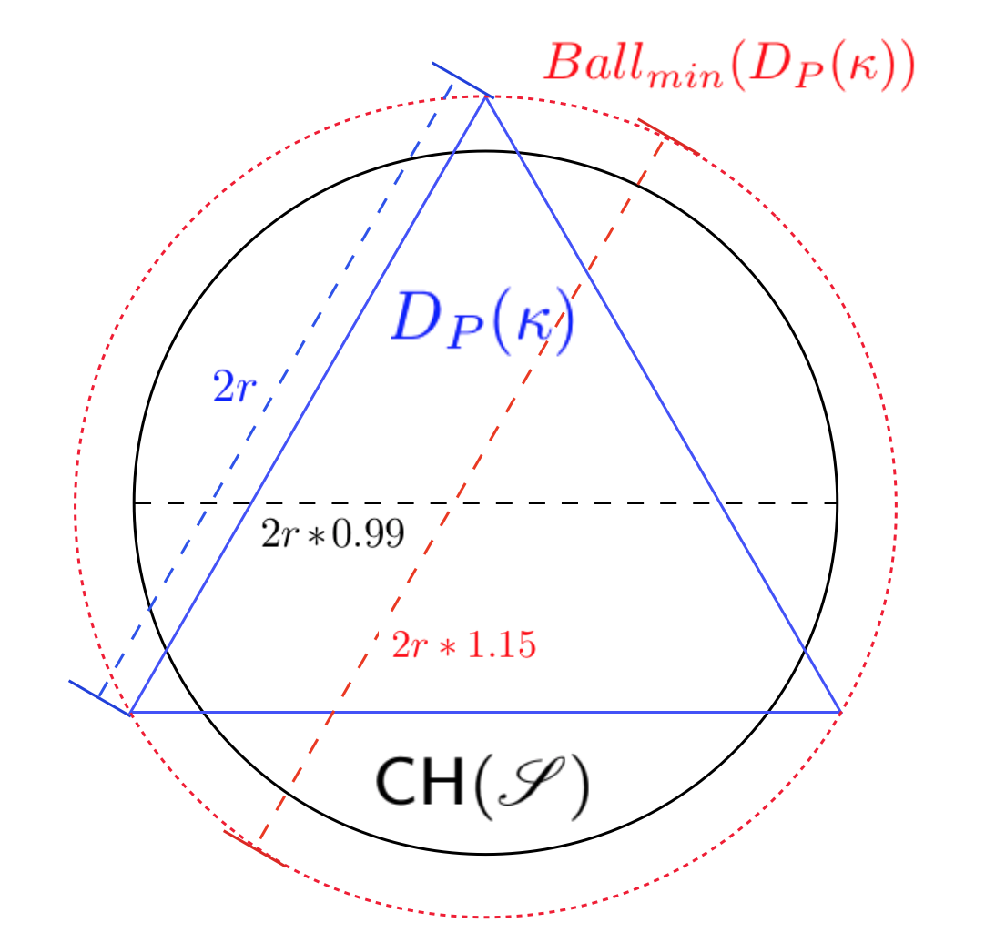
Refer to caption
Figure 2: An example showing that the property of Equation (11) doesn’t imply that (1−α)​DP​(κ)⊂𝖢𝖧⁡(𝒮)(1-\alpha)D_{P}(\kappa)\subset\mathsf{CH}(\mathcal{S}). Suppose DP​(κ)D_{P}(\kappa) is an equilateral triangle of edge-length 2​r2r and 𝒮\mathcal{S} happens to be a ball of diameter 2⋅0.99⋅r2\cdot 0.99\cdot r (and DP​(κ−Δ)D_{P}(\kappa-\Delta) is a much larger region). Note that 𝒮\mathcal{S} does satisfy Equation (11) for α=0.01\alpha=0.01 yet 0.99​DP​(κ)⊄𝖢𝖧⁡(𝒮)0.99D_{P}(\kappa)\nsubset\mathsf{CH}(\mathcal{S}). (E.g, the ball containing DP​(κ)D_{P}(\kappa) must have radius ≥23​r\geq\frac{2}{\sqrt{3}}r whereas 𝖢𝖧⁡(𝒮)\mathsf{CH}(\mathcal{S}) is contained inside a ball of radius 0.99​r0.99r.)

In our work, we give algorithms that satisfy variations of property (10). We give now the respective claims showing that each variation indeed yields a (α′,Δ)(\alpha^{\prime},\Delta)-kernel.

Claim 20.

Let 𝒮\mathcal{S} be a set that satisfies the following property in regards to DP​(κ)D_{P}(\kappa) and DP​(κ−Δ)D_{P}(\kappa-\Delta):

∀ direction u,maxp∈DP​(κ)⁡⟨p,u⟩−α⋅0​p​tκ≤maxp∈𝖢𝖧⁡(𝒮)⁡⟨p,u⟩≤maxp∈DP​(κ−Δ)⁡⟨p,u⟩+α⋅0​p​tκ−Δ\forall\textrm{ direction $u$,}~~~~~\max_{p\in D_{P}(\kappa)}\langle p,u\rangle-\alpha\cdot 0pt_{\kappa}\leq\max_{p\in\mathsf{CH}(\mathcal{S})}\langle p,u\rangle\leq\max_{p\in D_{P}(\kappa-\Delta)}\langle p,u\rangle+\alpha\cdot 0pt_{\kappa-\Delta} (12)

then, setting α′=2​α​d+12\alpha^{\prime}=2\alpha\sqrt{d+\frac{1}{2}}, there exists two vectors p1p_{1} and p2p_{2} s.t. we can shift DP​(κ)D_{P}(\kappa) and DP​(κ−Δ)D_{P}(\kappa-\Delta) and have that (1−α′)​(DP​(κ)−p1)⊂𝖢𝖧⁡(𝒮)−p1(1-\alpha^{\prime})(D_{P}(\kappa)-p_{1})\subset\mathsf{CH}(\mathcal{S})-p_{1} and 𝖢𝖧⁡(𝒮)−p2⊂(1+α′)​(DP​(κ−Δ)−p2)\mathsf{CH}({\mathcal{S}})-p_{2}\subset(1+\alpha^{\prime})(D_{P}(\kappa-\Delta)-p_{2}).

Proof.

We first argue about the relation between 𝖢𝖧⁡(𝒮)\mathsf{CH}({\mathcal{S}}) and DP​(κ−Δ)D_{P}(\kappa-\Delta). Denote the convex polytope DP​(κ−Δ)D_{P}(\kappa-\Delta) as the intersection of a finite number, kk, of closed half-spaces: {x∈ℝd:⟨x,vi⟩≤λi}\{x\in\mathbb{R}^{d}:\langle x,v_{i}\rangle\leq\lambda_{i}\}. We continue and leverage on the fact (see [GK92]) that any convex body with width ww must contain a ball of radius at least w​d+22​(d+1)\frac{w\sqrt{d+2}}{2(d+1)}. Let p2p_{2} be the center of this ball, and so DP​(κ−Δ)−p2D_{P}(\kappa-\Delta)-p_{2} is a shift of DP​(κ−Δ)D_{P}(\kappa-\Delta) where this ball is centered at the origin. Note that the origin is not only a point inside this shifted convex polytope, it is also a point of distance at least 0​p​tκ−Δ​d+22​d+2\frac{0pt_{\kappa-\Delta}\sqrt{d+2}}{2d+2} of all hyperplanes bounding it. Thus, based on for this particular shift, we can redefine the closed halfspaces and have that DP​(κ−Δ)=⋂i{x∈ℝd:⟨x−p2,vi⟩≤λi}D_{P}(\kappa-\Delta)=\bigcap_{i}\{x\in\mathbb{R}^{d}:\langle x-p_{2},v_{i}\rangle\leq\lambda_{i}\} where we also have that each λi≥0​p​tκ−Δ​d+22​d+2\lambda_{i}\geq\frac{0pt_{\kappa-\Delta}\sqrt{d+2}}{2d+2}.

For any closed halfspaced parameterized by vi,λiv_{i},\lambda_{i} we have that for any x∈𝖢𝖧⁡(𝒮)x\in\mathsf{CH}(\mathcal{S}) it holds that

⟨x−p2,vi⟩\displaystyle\langle x-p_{2},v_{i}\rangle ≤maxx∈𝖢𝖧⁡(𝒮)⁡⟨x,vi⟩−⟨p2,vi⟩≤maxx∈DP​(κ−Δ)⁡⟨x,vi⟩+α⋅w​i​d​t​hκ−Δ−⟨p2,vi⟩\displaystyle\leq\max_{x\in\mathsf{CH}(\mathcal{S})}\langle x,v_{i}\rangle-\langle p_{2},v_{i}\rangle\leq\max_{x\in D_{P}(\kappa-\Delta)}\langle x,v_{i}\rangle+\alpha\cdot width_{\kappa-\Delta}-\langle p_{2},v_{i}\rangle
=maxx∈DP​(κ−Δ)⁡⟨x−p2,vi⟩+α⋅0​p​tκ−Δ≤λi+2​d+2d+2​α​λi≤(1+2​α​d+12)​λi\displaystyle=\max_{x\in D_{P}(\kappa-\Delta)}\langle x-p_{2},v_{i}\rangle+\alpha\cdot 0pt_{\kappa-\Delta}\leq\lambda_{i}+\frac{2d+2}{\sqrt{d+2}}\alpha\lambda_{i}\leq(1+2\alpha\sqrt{d+\tfrac{1}{2}})\lambda_{i}

This proves that 𝖢𝖧⁡(𝒮)−p2⊂(1+α′)​(DP​(κ−Δ)−p2)\mathsf{CH}(\mathcal{S})-p_{2}\subset(1+\alpha^{\prime})(D_{P}(\kappa-\Delta)-p_{2}).

Next, we show that there exists p1p_{1} such that (1−α)​(DP​(κ)−p1)⊂𝖢𝖧⁡(𝒮)−p1(1-\alpha)(D_{P}(\kappa)-p_{1})\subset\mathsf{CH}(\mathcal{S})-p_{1}. We start by comparing 0​p​t​(𝖢𝖧⁡(𝒮))0pt(\mathsf{CH}(\mathcal{S})) to 0​p​tκ0pt_{\kappa}. Let uu be the direction on which the width of 𝖢𝖧⁡(𝒮)\mathsf{CH}(\mathcal{S}) is obtained. We thus have that

0​p​t​(𝖢𝖧⁡(𝒮))\displaystyle 0pt(\mathsf{CH}(\mathcal{S})) =maxa,b∈𝖢𝖧⁡(𝒮)⁡⟨a−b,u⟩=maxa∈𝖢𝖧⁡(𝒮)⁡⟨a,u⟩−minb∈𝖢𝖧⁡(𝒮)⁡⟨b,u⟩\displaystyle=\max_{a,b\in\mathsf{CH}(\mathcal{S})}\langle a-b,u\rangle=\max_{a\in\mathsf{CH}(\mathcal{S})}\langle a,u\rangle-\min_{b\in\mathsf{CH}(\mathcal{S})}\langle b,u\rangle
=maxa∈𝖢𝖧⁡(𝒮)⁡⟨a,u⟩+maxb∈𝖢𝖧⁡(𝒮)⁡⟨b,−u⟩\displaystyle=\max_{a\in\mathsf{CH}(\mathcal{S})}\langle a,u\rangle+\max_{b\in\mathsf{CH}(\mathcal{S})}\langle b,-u\rangle
≥maxa∈DP​(κ)⁡⟨a,u⟩+maxb∈DP​(κ)⁡⟨b,−u⟩−2​α⋅0​p​tκ\displaystyle\geq\max_{a\in D_{P}(\kappa)}\langle a,u\rangle+\max_{b\in D_{P}(\kappa)}\langle b,-u\rangle-2\alpha\cdot 0pt_{\kappa}
=maxa,b∈DP​(κ)⁡⟨a−b,u⟩−2​α⋅0​p​tκ≥0​p​tκ​(1−2​α)\displaystyle=\max_{a,b\in D_{P}(\kappa)}\langle a-b,u\rangle-2\alpha\cdot 0pt_{\kappa}\geq 0pt_{\kappa}(1-2\alpha)

This implies that in any direction uu we have that maxp∈DP​(κ)⁡⟨p,u⟩≤maxp∈𝖢𝖧⁡(𝒮)⁡⟨p,u⟩+α⋅0​p​tκ≤maxp∈𝖢𝖧⁡(𝒮)⁡⟨p,u⟩+α1−2​α⋅0​p​t​(𝖢𝖧⁡(𝒮))\max_{p\in D_{P}(\kappa)}\langle p,u\rangle\leq\max_{p\in\mathsf{CH}(\mathcal{S})}\langle p,u\rangle+\alpha\cdot 0pt_{\kappa}\leq\max_{p\in\mathsf{CH}(\mathcal{S})}\langle p,u\rangle+\frac{\alpha}{1-2\alpha}\cdot 0pt(\mathsf{CH}(\mathcal{S})). We can now apply the above argument and have that DP​(κ)−p1⊂(1+2​α1−2​α​d+12)​(𝖢𝖧⁡(𝒮)−p1)D_{P}(\kappa)~-~p_{1}~\subset(1+\frac{2\alpha}{1-2\alpha}\sqrt{d+\tfrac{1}{2}})(\mathsf{CH}(\mathcal{S})-p_{1}) for some p1p_{1}. Thus, (1−2​α​d+12)​(DP​(κ)−p1)⊂𝖢𝖧⁡(𝒮)−p1(1-{2\alpha}\sqrt{d+\tfrac{1}{2}})(D_{P}(\kappa)-p_{1})\subset\mathsf{CH}(\mathcal{S})-p_{1}. ∎

As discussed, our first algorithm yields a set 𝒮\mathcal{S} that (w.h.p.) satisfies the premise of Claim 20 and therefore it is a (α,Δ)(\alpha,\Delta)-kernel. Similarly, the second algorithm we provide (under slightly different conditions) yields the premise of the following claim.

Claim 21.

Fix α<1/6\alpha<1/6 and let 𝒮⊂DP​(κ−Δ)\mathcal{S}\subset D_{P}(\kappa-\Delta) be a set that satisfy the following property in regards to DP​(κ)D_{P}(\kappa). There exists a point c∈DP​(κ)∩𝒮c\in D_{P}(\kappa)\cap\mathcal{S} such that:

∀ direction u,(1−α)​maxp∈DP​(κ)​⟨p−c,u⟩≤maxp∈𝖢𝖧⁡(𝒮)⁡⟨p−c,u⟩+α⋅0​p​tκ\forall\textrm{ direction $u$,}~~~~~(1-\alpha)\max_{p\in D_{P}(\kappa)}\langle p-c,u\rangle\leq\max_{p\in\mathsf{CH}(\mathcal{S})}\langle p-c,u\rangle+\alpha\cdot 0pt_{\kappa} (13)

then there exists a vector bb such that we can shift DP​(κ)D_{P}(\kappa) and 𝖢𝖧⁡(𝒮)\mathsf{CH}(\mathcal{S}) by bb and have that

DP​(κ)−b⊂(1+α′)​(𝖢𝖧⁡(𝒮)−b)D_{P}(\kappa)-b\subset(1+\alpha^{\prime})\left(\mathsf{CH}(\mathcal{S})-b\right)

for α′=α1−α​(1+4​d+12)\alpha^{\prime}=\frac{\alpha}{1-\alpha}(1+4\sqrt{d+\frac{1}{2}}); and we also have that 𝖢𝖧⁡(𝒮)⊂DP​(κ−Δ)\mathsf{CH}({\mathcal{S}})\subset D_{P}(\kappa-\Delta). Thus, obviously, 𝒮\mathcal{S} is a (α′1+α′,Δ)\left(\frac{\alpha^{\prime}}{1+\alpha^{\prime}},\Delta\right)-kernel of DP​(κ)D_{P}(\kappa).

Proof.

First, since 𝒮⊂DP​(κ−Δ)\mathcal{S}\subset D_{P}(\kappa-\Delta) then it is obvious that 𝖢𝖧⁡(𝒮)⊂DP​(κ−Δ)\mathsf{CH}(\mathcal{S})\subset D_{P}(\kappa-\Delta). The difficulty lies in showing the first part.

We start by a similar argument to the one in the proof of Claim 20, comparing 0​p​t​(𝖢𝖧⁡(𝒮))0pt(\mathsf{CH}(\mathcal{S})) to 0​p​tκ0pt_{\kappa}. Let uu be the direction on which the width of 𝖢𝖧⁡(𝒮)\mathsf{CH}(\mathcal{S}) is obtained. We thus have that

0​p​t​(𝖢𝖧⁡(𝒮))\displaystyle 0pt(\mathsf{CH}(\mathcal{S})) =maxa,b∈𝖢𝖧⁡(𝒮)⁡⟨a−b,u⟩=maxa∈𝖢𝖧⁡(𝒮)⁡⟨a−c,u⟩−minb∈𝖢𝖧⁡(𝒮)⁡⟨b−c,u⟩\displaystyle=\max_{a,b\in\mathsf{CH}(\mathcal{S})}\langle a-b,u\rangle=\max_{a\in\mathsf{CH}(\mathcal{S})}\langle a-c,u\rangle-\min_{b\in\mathsf{CH}(\mathcal{S})}\langle b-c,u\rangle
=maxa∈𝖢𝖧⁡(𝒮)⁡⟨a−c,u⟩+maxb∈𝖢𝖧⁡(𝒮)⁡⟨b−c,−u⟩\displaystyle=\max_{a\in\mathsf{CH}(\mathcal{S})}\langle a-c,u\rangle+\max_{b\in\mathsf{CH}(\mathcal{S})}\langle b-c,-u\rangle
≥(1−α)​maxa∈DP​(κ)​⟨a−c,u⟩+(1−α)​maxb∈DP​(κ)​⟨b−c,−u⟩−2​α⋅0​p​tκ\displaystyle\geq(1-\alpha)\max_{a\in D_{P}(\kappa)}\langle a-c,u\rangle+(1-\alpha)\max_{b\in D_{P}(\kappa)}\langle b-c,-u\rangle-2\alpha\cdot 0pt_{\kappa}
=(1−α)​maxa,b∈DP​(κ)​⟨a−b,u⟩−2​α⋅0​p​tκ≥0​p​tκ​(1−3​α)\displaystyle=(1-\alpha)\max_{a,b\in D_{P}(\kappa)}\langle a-b,u\rangle-2\alpha\cdot 0pt_{\kappa}\geq 0pt_{\kappa}(1-3\alpha)

This implies that in any direction uu we have that maxp∈DP​(κ)⁡⟨p−c,u⟩≤11−α​maxp∈𝖢𝖧⁡(𝒮)​⟨p−c,u⟩+α1−α⋅0​p​tκ≤11−α​maxp∈𝖢𝖧⁡(𝒮)​⟨p−c,u⟩+α(1−α)​(1−3​α)⋅0​p​t​(𝖢𝖧⁡(𝒮))\max_{p\in D_{P}(\kappa)}\langle p-c,u\rangle\leq\frac{1}{1-\alpha}\max_{p\in\mathsf{CH}(\mathcal{S})}\langle p-c,u\rangle+\frac{\alpha}{1-\alpha}\cdot 0pt_{\kappa}\leq\frac{1}{1-\alpha}\max_{p\in\mathsf{CH}(\mathcal{S})}\langle p-c,u\rangle+\frac{\alpha}{(1-\alpha)(1-3\alpha)}\cdot 0pt(\mathsf{CH}(\mathcal{S})).

Now, based on a claim from [GK92], we know that 𝖢𝖧⁡(𝒮)\mathsf{CH}(\mathcal{S}) contains a ball, centered at some point zz, such that its radius is at least 0​p​t​(𝖢𝖧⁡(𝒮))​d+2(2​d+2)0pt(\mathsf{CH}(\mathcal{S}))\frac{\sqrt{d+2}}{(2d+2)}. Thus we denote the convex polytope 𝖢𝖧⁡(𝒮)\mathsf{CH}(\mathcal{S}) as 𝖢𝖧⁡(𝒮)=⋂i{x∈ℝd:⟨x−z,vi⟩≤λi}\mathsf{CH}(\mathcal{S})=\bigcap_{i}\{x\in\mathbb{R}^{d}:~\langle x-z,v_{i}\rangle\leq\lambda_{i}\} where for every ii it holds that λi≥0​p​t​(𝖢𝖧⁡(𝒮))​d+22​d+2≥0​p​tκ​(1−3​α)​d+22​d+2\lambda_{i}\geq 0pt(\mathsf{CH}(\mathcal{S}))\frac{\sqrt{d+2}}{2d+2}\geq 0pt_{\kappa}(1-3\alpha)\frac{\sqrt{d+2}}{2d+2}.

Set β=11+4​d+12∈[0,1]\beta=\frac{1}{1+4\sqrt{d+\frac{1}{2}}}\in[0,1], and denote b=(1−β)​z+β​cb=(1-\beta)z+\beta c. Note that b∈𝖢𝖧⁡(𝒮)b\in\mathsf{CH}(\mathcal{S}) due to convexity. Moreover, since for every viv_{i} it holds that ∀x,⟨x−z,vi⟩≤λi\forall x,\langle x-z,v_{i}\rangle\leq\lambda_{i} iff ⟨x−b,vi⟩≤λi+β⁡⟨z−c,vi⟩\langle x-b,v_{i}\rangle\leq\lambda_{i}+\beta\langle z-c,v_{i}\rangle, then we can rewrite 𝖢𝖧⁡(𝒮)\mathsf{CH}(\mathcal{S}) as 𝖢𝖧(𝒮)=∩i{x∈ℝd:⟨x−b,vi⟩≤λi+β⟨z−c,vi⟩}\mathsf{CH}(\mathcal{S})=\cap_{i}\{x\in\mathbb{R}^{d}:~\langle x-b,v_{i}\rangle\leq\lambda_{i}+\beta\langle z-c,v_{i}\rangle\}. So, as our goal is to show that DP​(κ)−b⊂(1+α′)​(𝖢𝖧⁡(𝒮)−b)D_{P}(\kappa)-b\subset(1+\alpha^{\prime})(\mathsf{CH}(\mathcal{S})-b). Namely, we show that all x∈DP​(κ)x\in D_{P}(\kappa) satisfy ⟨x−b,vi⟩≤(1+α′)​(λi+β⁡⟨z−c,vi⟩)\langle x-b,v_{i}\rangle\leq(1+\alpha^{\prime})\left(\lambda_{i}+\beta\langle z-c,v_{i}\rangle\right) for any vi,λiv_{i},\lambda_{i}.

Fix any closed halfspace parameterized by vi,λiv_{i},\lambda_{i} and any x∈DP​(κ)x\in D_{P}(\kappa). We have that

⟨x−b,vi⟩\displaystyle\langle x-b,v_{i}\rangle =⟨x−c,vi⟩+⟨c−b,vi⟩\displaystyle=\langle x-c,v_{i}\rangle+\langle c-b,v_{i}\rangle
≤11−α​maxp∈𝖢𝖧⁡(𝒮)​⟨p−c,vi⟩+α1−α⋅0​p​tκ+⟨c−b,vi⟩\displaystyle\leq\frac{1}{1-\alpha}\max_{p\in\mathsf{CH}(\mathcal{S})}\langle p-c,v_{i}\rangle+\frac{\alpha}{1-\alpha}\cdot 0pt_{\kappa}+\langle c-b,v_{i}\rangle
≤11−α​maxp∈𝖢𝖧⁡(𝒮)​⟨p−b,vi⟩+11−α​⟨b−c,vi⟩+λi​α⁡(2​d+2)(1−α)​(1−3​α)​d+2−⟨b−c,vi⟩\displaystyle\leq\frac{1}{1-\alpha}\max_{p\in\mathsf{CH}(\mathcal{S})}\langle p-b,v_{i}\rangle+\frac{1}{1-\alpha}\langle b-c,v_{i}\rangle+\lambda_{i}\frac{\alpha(2d+2)}{(1-\alpha)(1-3\alpha)\sqrt{d+2}}-\langle b-c,v_{i}\rangle
≤11−α​(λi+β⁡⟨z−c,vi⟩)+λi​α⁡(2​d+2)(1−α)​(1−3​α)​d+2+α1−α​⟨(1−β)​(z−c),vi⟩\displaystyle\leq\frac{1}{1-\alpha}\big(\lambda_{i}+\beta\langle z-c,v_{i}\rangle\big)+\lambda_{i}\frac{\alpha(2d+2)}{(1-\alpha)(1-3\alpha)\sqrt{d+2}}+\frac{\alpha}{1-\alpha}\langle(1-\beta)(z-c),v_{i}\rangle
=λi+λi​α1−α+λi​α⁡(2​d+2)(1−α)​(1−3​α)​d+2+β+α−α​β1−α​⟨z−c,vi⟩\displaystyle=\lambda_{i}+\lambda_{i}\frac{\alpha}{1-\alpha}+\lambda_{i}\frac{\alpha(2d+2)}{(1-\alpha)(1-3\alpha)\sqrt{d+2}}+\frac{\beta+\alpha-\alpha\beta}{1-\alpha}\langle z-c,v_{i}\rangle
=λi​[1+α1−α​(1+2​d+2(1−3​α)​d+2)]+(β+α1−α)​⟨z−c,vi⟩\displaystyle=\lambda_{i}\left[1+\frac{\alpha}{1-\alpha}\left(1+\frac{2d+2}{(1-3\alpha)\sqrt{d+2}}\right)\right]+\left(\beta+\frac{\alpha}{1-\alpha}\right)\langle z-c,v_{i}\rangle

Note that (1+α′)​β=(1+α1−α⋅1β)​β=β+α1−α(1+\alpha^{\prime})\beta=\left(1+\frac{\alpha}{1-\alpha}\cdot\frac{1}{\beta}\right)\beta=\beta+\frac{\alpha}{1-\alpha}. The key point here is that we have equality, not inequality, and this allows us to ignore partitioning into cases and see whether ⟨z−c,vi⟩\langle z-c,v_{i}\rangle is positive or not. Plugging in this equality into the above bound we get

⟨x−b,vi⟩\displaystyle\langle x-b,v_{i}\rangle ≤[1+α1−α​(1+2​d+2(1−3​α)​d+2)]​λi+(1+α′)​β​⟨z−c,vi⟩≤(1+α′)​λi+(1+α′)​β​⟨z−c,vi⟩\displaystyle\leq\left[1+\tfrac{\alpha}{1-\alpha}\left(1+\tfrac{2d+2}{(1-3\alpha)\sqrt{d+2}}\right)\right]\lambda_{i}+(1+\alpha^{\prime})\beta\langle z-c,v_{i}\rangle\leq(1+\alpha^{\prime})\lambda_{i}+(1+\alpha^{\prime})\beta\langle z-c,v_{i}\rangle

where the last inequality holds because λi>0\lambda_{i}>0 and because

α1−α​(1+2​d+2(1−3​α)​d+2)≤α′=α1−α​(1+4​d+12)\tfrac{\alpha}{1-\alpha}\left(1+\tfrac{2d+2}{(1-3\alpha)\sqrt{d+2}}\right)\leq\alpha^{\prime}=\tfrac{\alpha}{1-\alpha}(1+4\sqrt{d+\tfrac{1}{2}})

(Since α≤1/6\alpha\leq 1/6 then 2​d+2(1−3​α)​d+2≤4​d+1d+2≤4​d+12\frac{2d+2}{(1-3\alpha)\sqrt{d+2}}\leq 4\frac{d+1}{\sqrt{d+2}}\leq 4\sqrt{d+\frac{1}{2}}.) ∎

Definition of Fantess.

In the following subsection we detail our algorithms whose respective outputs satisfy the premise of Claims 20 and 21. Unfortunately, we were unable to find an algorithm that returns a kernel for any DP​(κ)D_{P}(\kappa). Much like in the non-private setting [AHV04], in order to give an algorithm that outputs a kernel of DP​(κ)D_{P}(\kappa) we must require DP​(κ)D_{P}(\kappa) satisfies a certain “fatness” property. In the standard, non-private setting, a convex polytope DP​(κ)D_{P}(\kappa) is called cdc_{d}-fat if there exists a constant cd≥1c_{d}\geq 1 (depends solely on the dimension dd) where diam⁡(DP​(κ))≤cd​0​p​t​(DP​(κ))\mathrm{diam}(D_{P}(\kappa))\leq c_{d}0pt(D_{P}(\kappa)) (see [AHV04]). Alas, our differentially private algorithm requires something stronger. Formally, we define the follow various notions of fatness.

Definition 22.

Given a dataset PP, we say that its κ\kappa-Tukey region is

  • •

    (cd,Δ)(c_{d},\Delta)-fat if it holds that 0​p​tκ≥1cd​diamκ−Δ0pt_{\kappa}\geq\tfrac{1}{c_{d}}\mathrm{diam}_{\kappa-\Delta}.

  • •

    (cd,Δ+,Δ−)(c_{d},\Delta_{+},\Delta_{-})-fat if it holds that 0​p​tκ+Δ+≥1cd​diamκ−Δ−0pt_{\kappa+\Delta_{+}}\geq\tfrac{1}{c_{d}}\mathrm{diam}_{\kappa-\Delta_{-}}.

  • •

    cdc_{d}-absolutely fat if 0​p​tκ≥1cd0pt_{\kappa}\geq\tfrac{1}{c_{d}}.

The following properties are immediate from the various definitions.

  • •

    If DP​(κ)D_{P}(\kappa) is (cd,Δ)(c_{d},\Delta)-fat then for any 0≤Δ′≤Δ0\leq\Delta^{\prime}\leq\Delta it is also (cd,Δ′)(c_{d},\Delta^{\prime})-fat. In particular it is also (cd,0)(c_{d},0)-fat which is the standard, non-private, definition of fatness.

  • •

    If DP​(κ)D_{P}(\kappa) is (cd,Δ)(c_{d},\Delta)-fat then for any cd′≥cdc_{d}^{\prime}\geq c_{d} it is also (cd′,Δ)(c_{d}^{\prime},\Delta)-fat.

  • •

    DP​(κ)D_{P}(\kappa) is (cd,Δ+,Δ−)(c_{d},\Delta_{+},\Delta_{-})-fat iff DP​(κ+Δ+)D_{P}(\kappa+\Delta_{+}) is (cd,(Δ++Δ−))(c_{d},(\Delta_{+}+\Delta_{-})~)-fat.

  • •

    If DP​(κ)D_{P}(\kappa) is (cd,Δ+,Δ−)(c_{d},\Delta_{+},\Delta_{-})-fat then for any Δ~+≤Δ+\tilde{\Delta}_{+}\leq\Delta_{+} and Δ~−≤Δ−\tilde{\Delta}_{-}\leq\Delta_{-} it holds that DP​(κ)D_{P}(\kappa) is also(cd,Δ~+,Δ~−)(c_{d},\tilde{\Delta}_{+},\tilde{\Delta}_{-})-fat.

  • •

    Since P⊂[0,1]dP\subset[0,1]^{d}, then for any κ′\kappa^{\prime} we have that diamκ′≤diam⁡(P)≤d\mathrm{diam}_{\kappa^{\prime}}\leq\mathrm{diam}(P)\leq\sqrt{d}. It follows that if DP​(κ)D_{P}(\kappa) is cdc_{d}-absolutely fat, then it is also (cd/d,Δ)(c_{d}/\sqrt{d},\Delta)-fat for any Δ\Delta.

Discussion.

It is clear that the fatness properties (i.e., non-private cdc_{d}-fat, (cd,Δ)(c_{d},\Delta)-fat, cdc_{d}-absolutely fat) can be violated by the addition or removal of a single datapoint to/from PP. Therefore, no differentially private algorithm can always assert w.h.p. whether DP​(κ)D_{P}(\kappa) is fat or not, nor estimate its fatness parameter cdc_{d}. We therefore proceed as follows. In the next few subsections we give our differentially private algorithms for fat Tukey-regions. That is, in Subsection 5.2 we assume that DP​(κ)D_{P}(\kappa) is cdc_{d}-absolutely fat and return a set 𝒮\mathcal{S} that satisfies the premise of Claim 20; and in Subsection 5.3 we assume DP​(κ)D_{P}(\kappa) is (cd,Δ)(c_{d},\Delta)-fat and return a set 𝒮\mathcal{S} which satisfies the premise of Claim 21. Moreover, in Subsection 5.4 we propose a heuristic that, assuming DP​(κ)D_{P}(\kappa) is (cd,κ1,κ2)(c_{d},\kappa_{1},\kappa_{2})-fat for some particular values of κ1,κ2\kappa_{1},\kappa_{2}, returns an estimation of cdc_{d}. But more importantly, in Sections 6 and 7 we show how to privately find a transformation TT that turns T​(DP​(κ))T(D_{P}(\kappa)) into a fat dataset. This transformation relies on the promise that vol⁡(DP​(κ))≥12​vol​(DP​(κ−Δ))\mathrm{vol}(D_{P}(\kappa))\geq\frac{1}{2}\mathrm{vol}(D_{P}(\kappa-\Delta)), a promise which DP​(κ)D_{P}(\kappa) may not satisfy. However, in Section 7 we show how to find a value κ∗\kappa^{*} where DP​(κ∗)D_{P}(\kappa^{*}) does satisfy this promise, allowing us to convert DP​(κ∗)D_{P}(\kappa^{*}) into a fat Tukey-region and then produce a kernel for DP​(κ∗)D_{P}(\kappa^{*}).

5.2 Private Kernel Approximation Under “Absolute Fatness”

In this section, we work under the premise that DP​(κ)D_{P}(\kappa) is cdc_{d}-absolutely fat, that is, that 0​p​tκ≥1/cd0pt_{\kappa}\geq 1/c_{d}. For some instances, we are able to privately check whether DP​(κ)D_{P}(\kappa) is cdc_{d}-absolutely fat — if it happens to be the case that DP​(κ+Δwidth)D_{P}(\kappa+\Delta^{\rm width}) is cdc_{d}-absolutely fat, we can apply Algorithm 3 and verify it is indeed the case. Moreover, even when DP​(κ)D_{P}(\kappa) isn’t absolutely-fat, in Sections 6 and 7 we discuss at length how to privately find a parameter κ\kappa and a mapping TT that transforms DP​(κ)D_{P}(\kappa) into a absolutely-fat Tukey-region.

For absolutely fat Tukey-regions, we are able to give a pretty simple algorithm: we traverse a fine enough grid and add a point to 𝒮\mathcal{S} if it is in a vicinity of a point in DP​(κ)D_{P}(\kappa). Details appear below.

Algorithm 6 Private Kernel Approximation of an Absolutely-Fat Tukey Region

Input: Dataset P⊂ℝdP\subset\mathbb{R}^{d}; Approximation parameter 0<α,β<1/20<\alpha,\beta<1/2; privacy parameters ε,δ>0\varepsilon,\delta>0; Tukey depth parameter κ\kappa and fatness parameter cdc_{d}.

1:  Set ζ←αcd​d\zeta\leftarrow\frac{\alpha}{c_{d}\sqrt{d}}. Let GζG_{\zeta} be the partitioning of the unit-cube [0,1]d[0,1]^{d} to subcubes of edge-length ζ\zeta.
2:  Set k←|Gζ|k\leftarrow|G_{\zeta}| and ε0←ε2​k​log⁡(1/δ)\varepsilon_{0}\leftarrow\frac{\varepsilon}{2\sqrt{k\log(1/\delta)}}, β0←βk\beta_{0}\leftarrow\frac{\beta}{k}.
3:  Init 𝒮←∅\mathcal{S}\leftarrow\emptyset.
4:  for each C∈GζC\in G_{\zeta} do
5:   if (maxx∈C⁡TD⁡(x,P)+YC≥κ−ln⁡(1/β0)ε0\max_{x\in C}\mathrm{TD}(x,P)+Y_{C}\geq\kappa-\frac{\ln(1/\beta_{0})}{\varepsilon_{0}} where YC∼𝖫𝖺𝗉⁡(𝟣ε𝟢)Y_{C}\sim\mathop{\mathsf{Lap(\frac{1}{\varepsilon_{0}})}}) then
6:    Add the center of CC to 𝒮\mathcal{S}.
7:   end if
8:  end for
9:  return 𝒮\mathcal{S}
Theorem 23.

Algorithm 6 is an efficient, (ε,δ)(\varepsilon,\delta)-DP algorithm that returns w.p. ≥1−β\geq 1-\beta a set 𝒮\mathcal{S} that satisfies for every direction uu that maxp∈DP​(κ)⁡⟨p,u⟩−α⋅0​p​tκ≤maxp∈𝒮⁡⟨p,u⟩≤maxp∈DP​(κ−Δkernel)⁡⟨p,u⟩−α⋅0​p​tκ−Δkernel\max_{p\in D_{P}(\kappa)}\langle p,u\rangle-\alpha\cdot 0pt_{\kappa}\leq\max_{p\in\mathcal{S}}\langle p,u\rangle\leq\max_{p\in D_{P}(\kappa-\Delta^{\rm kernel})}\langle p,u\rangle-\alpha\cdot 0pt_{\kappa-\Delta^{\rm kernel}}, where Δkernel=O⁡(d​(cd​dα)d/2​log⁡(1/δ)​log⁡(cd​dα​β)ε)\Delta^{\rm kernel}=O(\frac{d(\frac{c_{d}\sqrt{d}}{\alpha})^{d/2}\sqrt{\log(1/\delta)}\log(\frac{c_{d}d}{\alpha\beta})}{\varepsilon}).

Proof.

First, to see that Algorithm 6 is efficient, note that k=O⁡((cd​d/α)d)k=O((c_{d}\sqrt{d}/\alpha)^{d}). For each of the kk cubes in GζG_{\zeta} we find the largest κ′\kappa^{\prime} such that DP​(κ′)∩C≠∅D_{P}(\kappa^{\prime})\cap C\neq\emptyset using a LP, thus we are able to answer of the maxx∈C⁡TD⁡(x,P)\max_{x\in C}\mathrm{TD}(x,P) queries in poly\mathop{\mathrm{poly}}-time. (In fact, it is enough to check for each cube that some vertex of DP​(κ′)D_{P}(\kappa^{\prime}) exists on each of the 2​d2d-sides of the cube.)

Second, Algorithm 6 is clearly (ε,δ)(\varepsilon,\delta)-DP since it relies on kk queries, each with sensitivity of 11. Thus, “budgeting” the additive Laplace mechanism with privacy-loss parameter of ε0\varepsilon_{0} turns the entire algorithm to (ε,δ)(\varepsilon,\delta)-DP algorithm based on the advanced composition theorem [DRV10].

We continue under the event that for each C∈GζC\in G_{\zeta} we picked a random variable YCY_{C} such that |YC|≤ln⁡(1/β0)ε0|Y_{C}|\leq\frac{\ln(1/\beta_{0})}{\varepsilon_{0}}, an event we know to hold with probability ≥1−β\geq 1-\beta. Under this event, two things must occur: (i) for any CC where some xC∈Cx_{C}\in C has Tukey-depth ≥κ\geq\kappa we place a point yC∈𝒮y_{C}\in\mathcal{S}, and (ii) for any CC where we place its center point yC∈𝒮y_{C}\in\mathcal{S} there exists some zC∈Cz_{C}\in C with Tukey-depth of at least κ−2​ln⁡(1/β0)ε0=κ−Δkernel\kappa-\frac{2\ln(1/\beta_{0})}{\varepsilon_{0}}=\kappa-\Delta^{\rm kernel}. Note that ‖xC−yC‖,‖yC−zC‖≤d​(ζ2)2=α2​cd≤α​0​p​tκ2\|x_{C}-y_{C}\|,\|y_{C}-z_{C}\|\leq\sqrt{d(\frac{\zeta}{2})^{2}}=\frac{\alpha}{2c_{d}}\leq\frac{\alpha 0pt_{\kappa}}{2}.

We rely on these two implications to show that indeed we output a (α,Δkernel)(\alpha,\Delta^{\rm kernel})-kernel of DP​(κ)D_{P}(\kappa). Fix any direction uu. Let a∈DP​(κ)a\in D_{P}(\kappa) be the point that obtain the directional-max of DP​(κ)D_{P}(\kappa), and let yay_{a} be a point in 𝒮\mathcal{S} that is of distance ≤α⋅0​p​tκ2\leq\frac{\alpha\cdot 0pt_{\kappa}}{2} from aa. We thus have that

maxp∈DP​(κ)⁡⟨p,u⟩\displaystyle\max_{p\in D_{P}({\kappa})}\langle p,u\rangle =⟨a,u⟩=⟨ya,u⟩+⟨a−ya,u⟩\displaystyle=\langle a,u\rangle=\langle y_{a},u\rangle+\langle a-y_{a},u\rangle
≤⟨ya,u⟩+α⋅0​p​tκ2≤maxp∈𝒮⁡⟨p,u⟩+α⋅0​p​tκ\displaystyle\leq\langle y_{a},u\rangle+\frac{\alpha\cdot 0pt_{\kappa}}{2}\leq\max_{p\in\mathcal{S}}\langle p,u\rangle+\alpha\cdot 0pt_{\kappa}

Similarly, denote pp as the points in 𝒮\mathcal{S} that obtains the directional width along uu, and let zpz_{p} be a point of depth ≥κ−Δkernel\geq\kappa-\Delta^{\rm kernel} closest to pp. Again, we have that

maxz∈𝒮⁡⟨a,u⟩\displaystyle\max_{z\in\mathcal{S}}\langle a,u\rangle =⟨p,u⟩=⟨zp,u⟩+⟨p−zp,u⟩≤⟨zp,u⟩+α⋅0​p​tκ2\displaystyle=\langle p,u\rangle=\langle z_{p},u\rangle+\langle p-z_{p},u\rangle\leq\langle z_{p},u\rangle+\frac{\alpha\cdot 0pt_{\kappa}}{2}
≤maxp∈DP​(κ−Δkernel)⁡⟨p,u⟩+α⋅0​p​tκ−Δkernel​(u)≤(1+α)​wκ−Δkernel​(u)∎\displaystyle\leq\max_{p\in D_{P}(\kappa-\Delta^{\rm kernel})}\langle p,u\rangle+\alpha\cdot 0pt_{\kappa-\Delta^{\rm kernel}}(u)\leq(1+\alpha)w_{\kappa-\Delta^{\rm kernel}}(u)\qed

5.3 Private Kernel Approximation Under a (cd,Δ)(c_{d},\Delta)-Fatness Assumption

In this section we give a different algorithm for finding a (α,Δ)(\alpha,\Delta)-kernel of DP​(κ)D_{P}(\kappa) under the notion of (cd,Δ)(c_{d},\Delta)-fatness (recall Definition 22), namely that 0​p​tκ≥diamκ−Δcd0pt_{\kappa}\geq\frac{\mathrm{diam}_{\kappa-\Delta}}{c_{d}}. Why do we present this algorithm in addition to the previous one? After all, if we know that the given dataset is (cd,Δ)(c_{d},\Delta)-fat we can run Algorithm 2 to find an approximation of diamκ−Δ\mathrm{diam}_{\kappa-\Delta}, use the algorithm in Corollary 10 to find a point p∈DP​(κ)p\in D_{P}(\kappa), and then inflate the ball around pp and have that the resulting dataset is cdc_{d}-absolutely fat.

The answer is composed of several facts. First, the above-mentioned suggestion for turning DP​(κ)D_{P}(\kappa) into a cdc_{d}-absolutely fat might fail, since there are datasets where it may return a number much greater than diamκ−Δ\mathrm{diam}_{\kappa-\Delta}. (Recall, the guarantee of Algorithm 2 is based on diamκ−Δ\mathrm{diam}_{\kappa-\Delta} and diamκ−Δ−Δdiam\mathrm{diam}_{\kappa-\Delta-\Delta^{\mathrm{diam}}}, and the latter could potentially be much larger than the former.) But even if this was not the case, there are additional reasons for presenting a dedicated algorithm for (cd,Δ)(c_{d},\Delta)-fat Tukey regions. First and far most, there are datasets which are cdc_{d}-absolutely fat yet are (cd′,Δ)(c_{d}^{\prime},\Delta)-fat for a significantly smaller cd′<cdc_{d}^{\prime}<c_{d}. Secondly, under a certain regime of parameters it may yield a smaller Δ\Delta then Algorithm 6 — it is scaled down by a factor of dd/4​cd/αd^{d/4}\sqrt{c_{d}/\alpha} (which significant for the large cdc_{d} values we introduce) at the expense of added poly(d)\mathop{\mathrm{poly}}(d)-factors. In addition, the guarantee of the returned kernel 𝒮\mathcal{S} is slightly better: it actually satisfies that 𝒮⊂DP​(κ−Δ)\mathcal{S}\subset D_{P}(\kappa-\Delta), which makes it so that 𝖢𝖧⁡(𝒮)⊂DP​(κ−Δ)\mathsf{CH}(\mathcal{S})\subset D_{P}(\kappa-\Delta) (without the rescaling by a factor of (1+α)(1+\alpha) and without some unknown shift).

So throughout this section, we assume we know that for the given κ\kappa, our input dataset is (cd,Δ)(c_{d},\Delta)-fat and so we produce a (α,Δ)(\alpha,\Delta)-kernel for it (for the same value of Δ\Delta). In fact, in order to avoid confusion with the definition of Δkernel\Delta^{\rm kernel} from Theorem 23, we denote the change to the Tukey depth by Γkernel\Gamma^{\rm kernel} in this subsection and the following.

The algorithm we discuss here mimics its non-private kernel analogue, where one uses a ζ\zeta-angle cover VζV_{\zeta} of the unit-sphere, with ζ≈αcd\zeta\approx{\frac{\alpha}{c_{d}}}. We start by finding some c∈DP​(κ)c\in D_{P}(\kappa) using the algorithm from Corollary 10. Then, iterating through all directions in VζV_{\zeta}, we find a point in DP​(κ−Γkernel)D_{P}(\kappa-\Gamma^{\rm kernel}) which approximately maximizes the projection along the given direction. Our algorithm is thus provided below.

Algorithm 7 Private Kernel Approximation of a (cd,Δ)(c_{d},\Delta)-Fat Tukey Region

Input: Dataset P⊂ℝdP\subset\mathbb{R}^{d}; Approximation parameter 0<α,β<1/20<\alpha,\beta<1/2; privacy parameters ε>0,δ≥0\varepsilon>0,\delta\geq 0; Tukey depth parameter κ\kappa and fatness parameter cdc_{d}.

1:  Set ζ←min⁡{α2​2​cd,1/2}\zeta\leftarrow\min\{{\frac{\alpha}{2\sqrt{2}c_{d}}},1/2\}. Let VζV_{\zeta} be a ζ\zeta-angle cover of the unit sphere of size 2​(π/ζ)d−12(\pi/\zeta)^{d-1}.
2:  Set k←d⁡(|Vζ|+1)k\leftarrow d(|V_{\zeta}|+1) and ε0←ε2​k​log⁡(2/δ)\varepsilon_{0}\leftarrow\frac{\varepsilon}{2\sqrt{k\log(2/\delta)}}, δ0←δ2​k\delta_{0}\leftarrow\frac{\delta}{2k}, β0←βk\beta_{0}\leftarrow\frac{\beta}{k}.
3:  Find c∈DP​(κ)c\in D_{P}(\kappa) by setting κ∗=κ+d​αqc​(ε0,δ0,β0)\kappa^{*}=\kappa+d\alpha^{\rm qc}(\varepsilon_{0},\delta_{0},\beta_{0}) and applying the algorithm from Corollary 10 with κ∗\kappa^{*}.
4:  Init 𝒮←{c}\mathcal{S}\leftarrow\{c\}.
5:  for each v∈Vζv\in V_{\zeta} do
6:   Compute ℓv←𝙳𝙿𝙼𝚊𝚡𝙿𝚛𝚘𝚓𝚎𝚌𝚝𝚒𝚘𝚗⁡(ε0,β0,c,v,κ)\ell_{v}\leftarrow{\tt DPMaxProjection}(\varepsilon_{0},\beta_{0},c,v,\kappa) approximated to a factor of (1−α)(1-\alpha).
7:   Using the rotation RvR_{v} that maps vv as the first standard axis, complete the first coordinate x=⟨c,v⟩+ℓvx=\langle c,v\rangle+\ell_{v} to a point qvq_{v} by applying 𝖳𝖣𝖢⁡(ε0,δ0,β0)\mathsf{TDC}(\varepsilon_{0},\delta_{0},\beta_{0}) for d−1d-1 times.Add qvq_{v} to 𝒮\mathcal{S}.
8:  end for
9:  return the pair (c,𝒮)(c,\mathcal{S})
Theorem 24.

Given ε>0,δ>0,α>0,β>0\varepsilon>0,\delta>0,\alpha>0,\beta>0 and cd≥1c_{d}\geq 1, set

Γcdkernel={O⁡(d32​(cdα)d−12​log⁡(1δ)​(υ+d​log⁡(d​cd/α​β))ε),using ε-DP binary-searchO~​(d52​(cdα)d−12​log⁡(1δ)​log⁡(υ​d​cd/ε​δ​α​β)ε),using “Between Thresholds”O⁡(d52​(cdα)d−12​log⁡(1δ)​log⁡(d​cd​υα​β​δ)​8log∗⁡(υ)​log∗⁡(υ)ε),using “RecConcave”\Gamma^{\rm kernel}_{c_{d}}=\begin{cases}O(\frac{d^{\frac{3}{2}}(\frac{c_{d}}{\alpha})^{\frac{d-1}{2}}\sqrt{\log(\frac{1}{\delta})}\big(\upsilon+d\log(dc_{d}/\alpha\beta)\big)}{\varepsilon}),&~\textrm{using $\varepsilon$-DP binary-search}\\ \tilde{O}(\frac{d^{\frac{5}{2}}(\frac{c_{d}}{\alpha})^{\frac{d-1}{2}}\sqrt{\log(\frac{1}{\delta})}\log(\upsilon dc_{d}/\varepsilon\delta\alpha\beta)}{\varepsilon}),&~\textrm{using ``Between Thresholds''}\\ O\left(\frac{d^{\frac{5}{2}}(\frac{c_{d}}{\alpha})^{\frac{d-1}{2}}\sqrt{\log(\frac{1}{\delta})}\log(\frac{dc_{d}\upsilon}{\alpha\beta\delta})8^{\log^{*}(\upsilon)}\log^{*}(\upsilon)}{\varepsilon}\right),&~\textrm{using ``RecConcave''}\end{cases} (14)

Let P⊂𝒢dP\subset\mathcal{G}^{d} be a dataset where (i) for κ∗=κ+d​αqc​(ε0,δ0,β0)\kappa^{*}=\kappa+d\alpha^{\rm qc}(\varepsilon_{0},\delta_{0},\beta_{0}), its κ∗\kappa^{*}-Tukey region is non empty, and (ii) its κ\kappa-Tukey region is (cd,Γcdkernel)(c_{d},\Gamma_{c_{d}}^{\rm kernel})-fat. Then Algorithm 7 is an efficient (ε,δ)(\varepsilon,\delta)-differentially private algorithm that when applied to PP returns w.p. ≥1−β\geq 1-\beta a set 𝒮\mathcal{S} and a point c∈𝒮c\in\mathcal{S} which satisfies (i) 𝒮⊂DP​(κ−Γkernel)\mathcal{S}~\subset~D_{P}(\kappa-\Gamma^{\rm kernel}) and (ii) for every direction uu it holds that (1−α)​maxp∈DP​(κ)​⟨p−c,u⟩≤maxp∈𝒮⁡⟨p−c,u⟩+α⋅0​p​tκ(1-\alpha)\max_{p\in D_{P}(\kappa)}\langle p-c,u\rangle\leq\max_{p\in\mathcal{S}}\langle p-c,u\rangle+\alpha\cdot 0pt_{\kappa}.

Proof.

First, we argue this algorithm is efficient. This is clear, since VζV_{\zeta} is of size ∝(cd/α)d−1\propto(c_{d}/\alpha)^{d-1} and (initially and) for each direction we run an efficient 𝖳𝖣𝖢\mathsf{TDC}-function (as discussed in Section 3).

Second, this algorithm is (ε,δ)(\varepsilon,\delta)-DP due to the advanced composition theorem of [DRV10], and the fact that overall we apply kk (ε0,δ0)(\varepsilon_{0},\delta_{0})-differentially private subprocedures. Furthermore, since each subprocedure has a probability of β0\beta_{0} of failure, we continue this proof under the assumption that no subroutine has failed and all guarantees are satisfied, which happens with probability ≥1−k​β0=1−β\geq 1-k\beta_{0}=1-\beta.

We thus have that cc has Tukey depth of ≥κ∗−d​αqc​(ε0,δ0,β0)=κ\geq\kappa^{*}-d\alpha^{\rm qc}(\varepsilon_{0},\delta_{0},\beta_{0})=\kappa thus c∈DP​(κ)c\in D_{P}(\kappa). Moreover, for each direction v∈Vζv\in V_{\zeta} we have ℓv\ell_{v} satisfies (1−α)​maxp∈DP​(κ)​⟨p−c,v⟩≤ℓv≤maxp∈DP​(κ−Δmax−proj​(ε0,β0))(1-\alpha)\max_{p\in D_{P}(\kappa)}\langle p-c,v\rangle\leq\ell_{v}\leq\max_{p\in D_{P}(\kappa-\Delta^{\rm max-proj}(\varepsilon_{0},\beta_{0}))} where Δmax−proj​(ε0,β0)=O⁡(log⁡(υ+log⁡(d)α​β0)ε0)=O⁡(k​log⁡(1/δ)​log⁡(k⁡(υ+log⁡(d))α​β)ε)\Delta^{\rm max-proj}(\varepsilon_{0},\beta_{0})=O(\frac{\log(\frac{\upsilon+\log(d)}{\alpha\beta_{0}})}{\varepsilon_{0}})=O(\frac{\sqrt{k\log(1/\delta)}\log(\frac{k(\upsilon+\log(d))}{\alpha\beta})}{\varepsilon}) by Theorem 17. As k=O⁡(d​(cdα)(d−1))k=O(d(\frac{c_{d}}{\alpha})^{({d-1})}) we get that Δmax−proj=O⁡(d3​(cdα)d−12​log⁡(υ​d​cd/α​β)​log⁡(1/δ)ε)\Delta^{\rm max-proj}=O(\frac{\sqrt{d^{3}}(\frac{c_{d}}{\alpha})^{\frac{d-1}{2}}\log(\upsilon dc_{d}/\alpha\beta)\sqrt{\log(1/\delta)}}{\varepsilon}). Then, by Corollary 10 we have that the point qvq_{v} retrieved for direction vv have Tukey-depth of κ−Δmax−proj−(d−1)​αqc​(ε0,δ0,β0)=κ−Γkernel\kappa-\Delta^{\rm max-proj}-(d-1)\alpha^{\rm qc}(\varepsilon_{0},\delta_{0},\beta_{0})=\kappa-\Gamma^{\rm kernel} where

Γkernel\displaystyle\Gamma^{\rm kernel} =O⁡(d32​(cdα)d−12​log⁡(υ​d​cd/α​β)​log⁡(1δ)ε)+O⁡(d​αqc​(εd​log⁡(1δ)​(cdα)d−12,δd​(cdα)d−1,βd​(cdα)d−1))\displaystyle=O(\frac{d^{\frac{3}{2}}(\frac{c_{d}}{\alpha})^{\frac{d-1}{2}}\log(\upsilon dc_{d}/\alpha\beta)\sqrt{\log(\frac{1}{\delta})}}{\varepsilon})+O(d\alpha^{\rm qc}(\frac{\varepsilon}{\sqrt{d\log(\frac{1}{\delta})}(\frac{c_{d}}{\alpha})^{\frac{d-1}{2}}},\frac{\delta}{d(\frac{c_{d}}{\alpha})^{{d-1}}},\frac{\beta}{d(\frac{c_{d}}{\alpha})^{{d-1}}}))
=O⁡(d32​(cdα)d−12​log⁡(υ​d​cd/α​β)​log⁡(1/δ)ε)+{O⁡(d​d​log⁡(1/δ)​(cdα)d−12​(υ+log⁡(d​(cdα)d−1/β))ε)O~​(d​d​log⁡(1/δ)​(cdα)d−12​log⁡(d2​(cdα)2​(d−1)​υ/β​ε​δ)ε)O⁡(d​d​log⁡(1/δ)​(cdα)d−12​8log∗⁡(υ)​log∗⁡(υ)⋅log⁡(d2​(cdα)2​(d−1)​log∗⁡(υ)β​δ)ε)\displaystyle=O(\frac{d^{\frac{3}{2}}(\frac{c_{d}}{\alpha})^{\frac{d-1}{2}}\log(\upsilon dc_{d}/\alpha\beta)\sqrt{\log(1/\delta)}}{\varepsilon})+\begin{cases}O(\frac{d\sqrt{d\log(1/\delta)}(\frac{c_{d}}{\alpha})^{\frac{d-1}{2}}(\upsilon+\log(d(\frac{c_{d}}{\alpha})^{{d-1}}/\beta))}{\varepsilon})\\ \tilde{O}(\frac{d\sqrt{d\log(1/\delta)}(\frac{c_{d}}{\alpha})^{\frac{d-1}{2}}\log(d^{2}(\frac{c_{d}}{\alpha})^{2(d-1)}\upsilon/\beta\varepsilon\delta)}{\varepsilon})\\ O\left(\frac{d\sqrt{d\log(1/\delta)}(\frac{c_{d}}{\alpha})^{\frac{d-1}{2}}8^{\log^{*}(\upsilon)}\log^{*}(\upsilon)\cdot\log(\frac{d^{2}(\frac{c_{d}}{\alpha})^{2(d-1)}\log^{*}(\upsilon)}{\beta\delta})}{\varepsilon}\right)\end{cases}
={O⁡(d32​(cdα)d−12​log⁡(1δ)​(υ+d​log⁡(d​cd/α​β))ε),using ε-DP binary-searchO~​(d52​(cdα)d−12​log⁡(1δ)​log⁡(υ​d​cd/ε​δ​α​β)ε),using “Between Thresholds”O⁡(d52​(cdα)d−12​log⁡(1δ)​log⁡(d​cd​υα​β​δ)​8log∗⁡(υ)​log∗⁡(υ)ε),using “RecConcave”\displaystyle=\begin{cases}O(\frac{d^{\frac{3}{2}}(\frac{c_{d}}{\alpha})^{\frac{d-1}{2}}\sqrt{\log(\frac{1}{\delta})}\big(\upsilon+d\log(dc_{d}/\alpha\beta)\big)}{\varepsilon}),&~\textrm{using $\varepsilon$-DP binary-search}\\ \tilde{O}(\frac{d^{\frac{5}{2}}(\frac{c_{d}}{\alpha})^{\frac{d-1}{2}}\sqrt{\log(\frac{1}{\delta})}\log(\upsilon dc_{d}/\varepsilon\delta\alpha\beta)}{\varepsilon}),&~\textrm{using ``Between Thresholds''}\\ O\left(\frac{d^{\frac{5}{2}}(\frac{c_{d}}{\alpha})^{\frac{d-1}{2}}\sqrt{\log(\frac{1}{\delta})}\log(\frac{dc_{d}\upsilon}{\alpha\beta\delta})8^{\log^{*}(\upsilon)}\log^{*}(\upsilon)}{\varepsilon}\right),&~\textrm{using ``RecConcave''}\end{cases}

And so, it follows that 𝒮⊂DP​(κ−Γkernel)\mathcal{S}\subset D_{P}(\kappa-\Gamma^{\rm kernel}).

Next, we argue that for any u∈𝕊d−1u\in\mathbb{S}^{d-1} it holds that (1−α)​maxp∈DP​(κ)​⟨p−c,u⟩≤maxp∈𝒮⁡⟨p−c,u⟩+α⋅0​p​tκ(1-\alpha)\max_{p\in D_{P}(\kappa)}\langle p-c,u\rangle\leq\max_{p\in\mathcal{S}}\langle p-c,u\rangle+\alpha\cdot 0pt_{\kappa} for the point cc chosen by the algorithm (which we know to be in DP​(κ)D_{P}(\kappa)). Fix any direction uu. Let p∗∈DP​(κ)p^{*}\in D_{P}(\kappa) be the point obtaining maxp∈DP​(κ)⁡⟨p−c,u⟩\max_{p\in D_{P}(\kappa)}\langle p-c,u\rangle and denote mu=⟨p∗−c,u⟩m_{u}=\langle p^{*}-c,u\rangle. Denote v∈Vζv\in V_{\zeta} as the nearest direction (of angle at most ζ\zeta) to uu, and recall that ‖u−v‖≤2​ζ≤α2​cd\|u-v\|\leq\sqrt{2}\zeta\leq\frac{\alpha}{2c_{d}}. It follows that

⟨p∗−c,v⟩=⟨p∗−c,u⟩+⟨p∗−c,v−u⟩≥mu−‖p∗−c‖​‖u−v‖≥mu−α​diamκ2​cd\langle p^{*}-c,v\rangle=\langle p^{*}-c,u\rangle+\langle p^{*}-c,v-u\rangle\geq m_{u}-\|p^{*}-c\|\|u-v\|\geq m_{u}-\frac{\alpha\mathrm{diam}_{\kappa}}{2c_{d}}

As a result, it holds that maxp∈DP​(κ)⁡⟨p−c,v⟩≥mu−α​diamκ2​cd\max_{p\in D_{P}(\kappa)}\langle p-c,v\rangle\geq m_{u}-\frac{\alpha\mathrm{diam}_{\kappa}}{2c_{d}} and thus ℓv≥(1−α)​(mu−α​diamκ2​cd)\ell_{v}\geq(1-\alpha)(m_{u}-\frac{\alpha\mathrm{diam}_{\kappa}}{2c_{d}}). Let qvq_{v} be the point in 𝒮⊂DP​(κ−Γkernel)\mathcal{S}\subset D_{P}(\kappa-\Gamma^{\rm kernel}) which we picked for direction vv and whose projection onto vv is precisely ℓv+⟨c,v⟩\ell_{v}+\langle c,v\rangle. We therefore have that Thus,

maxq∈𝒮⁡⟨q−c,u⟩\displaystyle\max\limits_{q\in\mathcal{S}}\langle q-c,u\rangle ≥⟨qv−c,u⟩=⟨qv−c,v⟩+⟨qv−c,u−v⟩≥ℓv−diamκ−Γkernel​‖u−v‖\displaystyle\geq\langle q_{v}-c,u\rangle=\langle q_{v}-c,v\rangle+\langle q_{v}-c,u-v\rangle\geq\ell_{v}-\mathrm{diam}_{\kappa-\Gamma^{\rm kernel}}\|u-v\|
≥(1−α)​(mu−α​diamκ2​cd)−diamκ−Γkernel​α2​cd\displaystyle\geq(1-\alpha)(m_{u}-\frac{\alpha\mathrm{diam}_{\kappa}}{2c_{d}})-\mathrm{diam}_{\kappa-\Gamma^{\rm kernel}}\frac{\alpha}{2c_{d}}
≥(1−α)​mu−α⁡(diamκ+diamκ−Γkernel)2​cd≥(1−α)​mu−2​α⋅diamκ−Γkernel2​cd\displaystyle\geq(1-\alpha)m_{u}-\frac{\alpha(\mathrm{diam}_{\kappa}+\mathrm{diam}_{\kappa-\Gamma^{\rm kernel}})}{2c_{d}}\geq(1-\alpha)m_{u}-\frac{2\alpha\cdot\mathrm{diam}_{\kappa-\Gamma^{\rm kernel}}}{2c_{d}}
≥fatness(1−α)​mu−α⋅0​p​tκ\displaystyle\stackrel{{\scriptstyle\rm fatness}}{{\geq}}(1-\alpha)m_{u}-\alpha\cdot 0pt_{\kappa}

∎

5.4 Coping with the Relation between cdc_{d} and Γcdkernel\Gamma_{c_{d}}^{\rm kernel}

Theorem 24 implies that we are able to privately output a (α,Γkernel)(\alpha,\Gamma^{\rm kernel})-kernel for datasets which are a-priori guaranteed to be (cd,Γkernel)(c_{d},\Gamma^{\rm kernel})-fat, where Γcdkernel\Gamma^{\rm kernel}_{c_{d}} is a function of multiple parameters, including cdc_{d}. Yet, when cdc_{d} is not a-priori given, it is unclear how to verify the “right” cdc_{d}, seeing as it is unclear the diameter of which Tukey-region κ′=κ−Γ⁡(cd)\kappa^{\prime}=\kappa-\Gamma(c_{d}) we should compare to the width of DP​(κ)D_{P}(\kappa). The non-private approach would be to try multiple values of cdc_{d} but this leads to multiple (sensitive) queries about the input.

We offer two solutions to this problem. One is a heuristic, and so — while we believe it does work for many datasets — it is not guaranteed to always work. This is the solution we discuss in this section. The other, which is guaranteed to work but involves choosing a particular κ\kappa, is discussed at length in the following sections.

The heuristic we pose here is based on the work of Liu and Talwar [LT19]. Basically, we traverse each option of cdc_{d}, here in powers of 22, up to cmax=4​d5/2⋅5d⋅(d!)c_{\max}=4d^{5/2}\cdot 5^{d}\cdot(d!) (in Section 6 the choice for this particular parameter is explained), and for each value check whether the diameter of the suitable DP​(κ−Γkernel)D_{P}(\kappa-\Gamma^{\rm kernel}) is upper bounded by cd⋅0​p​tκc_{d}\cdot 0pt_{\kappa} or not.

Formally, we set t=⌈log2⁡(cmax)⌉=⌈log2⁡(4​d5/2⋅5d⋅(d!))⌉t=\lceil\log_{2}(c_{\max})\rceil=\lceil\log_{2}(4d^{5/2}\cdot 5^{d}\cdot(d!))\rceil as the number of levels we test. For each 1≤i≤t1\leq i\leq t let MiM_{i} be the 2​ε2\varepsilon-DP mechanism that works as follows:

  1. 1.

    Set ci=2ic_{i}=2^{i}, set Γi=Γcikernel\Gamma_{i}=\Gamma^{\rm kernel}_{c_{i}} according to Theorem 24.

  2. 2.

    Run Algorithm 2 with Tukey-depth parameter of κi1=κ−Γi\kappa_{i}^{1}=\kappa-\Gamma_{i} and failure probability of β12​t​ln⁡(2/β)\frac{\beta}{12t\ln(2/\beta)}. Denote the result DD, and by Theorem 13 we know that w.p. ≥1−β12​t​ln⁡(2/β)\geq 1-\frac{\beta}{12t\ln(2/\beta)} it holds that D≥(1−α)​diamκ−ΓiD\geq(1-\alpha)\mathrm{diam}_{\kappa-\Gamma_{i}}.

  3. 3.

    Run Algorithm 3 with a lower bound of B=D/ciB=D/c_{i}, with Tukey-depth parameter of κ2=κ+Δ0​p​t​(ε,β12​t​ln⁡(2β))=κ+O⁡(log⁡(t⁡(υ+log⁡(d))α​β)ε)\kappa_{2}=\kappa+\Delta^{0pt}(\varepsilon,\frac{\beta}{12t\ln(\frac{2}{\beta})})=\kappa+O(\frac{\log(\frac{t(\upsilon+\log(d))}{\alpha\beta})}{\varepsilon}) as defined in Theorem 15, and with failure probability of β12​t​ln⁡(2/β)\frac{\beta}{12t\ln(2/\beta)}. Denote the result ww, and by Theorem 15 we know that w.p. ≥1−β12​t​ln⁡(2/β)\geq 1-\frac{\beta}{12t\ln(2/\beta)} it holds that w≤(1+α)​0​p​tκw\leq(1+\alpha)0pt_{\kappa} if w≠0w\neq 0.

  4. 4.

    return the tuple (i,τ)(i,\tau) when the score τ\tau is set be τ=2−i\tau=2^{-i} if D≤ci​1−α1+α​wD\leq c_{i}\frac{1-\alpha}{1+\alpha}w, or set as τ=0\tau=0 if any of the returned values is 00 or if D>ci​1−α1+α​wD>c_{i}\frac{1-\alpha}{1+\alpha}w.

As in the work of Liu and Talwar [LT19] we define the 2​ε2\varepsilon-DP algorithm QQ which picks i∈[t]i\in[t] u.a.r and runs MiM_{i}. Setting γ=1/3​t\gamma=1/3t, we define Q~\tilde{Q} as the mechanism that works as follows:

  • •

    Repeat:

    1. 1.

      Run QQ, namely pick i∈[t]i\in[t] u.a.r and add its output Mi​(P)M_{i}(P) to a (multi-)set SS.

    2. 2.

      Toss a biased coin: w.p. γ\gamma output an element in SS with maximal τ\tau and halt.

Applying Theorem 3.2 from [LT19], we infer that Q~\tilde{Q} is 6​ε6\varepsilon-DP. Moreover, we can argue the following about its utility.

Claim 25.

W.p. ≥1−β\geq 1-\beta, if Q~\tilde{Q} returns an index ii with score τ>0\tau>0 then DP​(κ)D_{P}(\kappa) is (ci,Γi)(c_{i},\Gamma_{i})-fat. Furthermore, denote

G​o​o​d={1≤i≤t:DP​(κ)​ is ​(1−α1+α​ci,Δ0​p​t​(ε,β12​t​ln⁡(2β)),Γi+Δdiam​(ε,β12​t​ln⁡(2β)))​-fat}Good=\{1\leq i\leq t:D_{P}(\kappa)\textrm{ is }\big(\tfrac{1-\alpha}{1+\alpha}c_{i},\Delta^{0pt}(\varepsilon,\tfrac{\beta}{12t\ln(\frac{2}{\beta})}),\Gamma_{i}+\Delta^{\mathrm{diam}}(\varepsilon,\tfrac{\beta}{12t\ln(\frac{2}{\beta})})\big)\textrm{-fat}\}

If G​o​o​d≠∅Good\neq\emptyset then, assuming β<1/6\beta<1/6, w.p. ≥1/2\geq 1/2 the mechanism Q~\tilde{Q} returns i≤min{i∈Good}i\leq\min\{i\in Good\}.

Proof.

First, algorithm Q~\tilde{Q} halts the very first time its biased coin comes up heads. Clearly, the probability it iterates for ≥ln⁡(2/β)/γ=3​t​ln⁡(2/β)\geq\ln(2/\beta)/\gamma=3t\ln(2/\beta) is at most (1−γ)ln⁡(2/β)/γ≤e−ln⁡(2/β)≤β/2(1-\gamma)^{\ln(2/\beta)/\gamma}\leq e^{-\ln(2/\beta)}\leq\beta/2. Second, since we set the failure probability of each MiM_{i} to be upper bounded by 2⋅β/(12​t​ln⁡(2/β))2\cdot\beta/(12t\ln(2/\beta)) then the probability that in any of the ≤3​t​(ln⁡(2/β))\leq 3t(\ln(2/\beta)) iterations one of the executed MiM_{i} fails is at most β/2\beta/2. It follows that w.p. ≥1−β\geq 1-\beta the algorithm Q~\tilde{Q} returns some score of some successfully executed MiM_{i}.

We continue under the assumption that this event indeed holds. Now, if Q~\tilde{Q} returns ii with τ>0\tau>0 it follows that for this ii it indeed holds that (1−α)​diamκ−Γi≤D≤ci​1−α1+α​w≤(1−α)​ci​0​p​tκ(1-\alpha)\mathrm{diam}_{\kappa-\Gamma_{i}}\leq D\leq c_{i}\frac{1-\alpha}{1+\alpha}w\leq(1-\alpha)c_{i}{0pt_{\kappa}}, and so diamκ−Γi≤ci​0​p​tκ\mathrm{diam}_{\kappa-\Gamma_{i}}\leq c_{i}0pt_{\kappa}, hence DP​(κ)D_{P}(\kappa) if (ci,Γi)(c_{i},\Gamma_{i})-fat.

Next, assume G​o​o​d≠∅Good\neq\emptyset and consider i∗=min{i∈Good}i^{*}=\min\{i\in Good\}. If indeed Mi∗M_{i^{*}} is executed and no failure occurs then it must be that D≤diamκ−Γi−Δdiam​(ε,β12​t​ln⁡(2β))D\leq\mathrm{diam}_{\kappa-\Gamma_{i}-\Delta^{\mathrm{diam}}(\varepsilon,\frac{\beta}{12t\ln(\frac{2}{\beta})})}; similarly, it must be that w≥0​p​tκ+Δ0​p​t​(ε,β12​t​ln⁡(2β))w\geq 0pt_{\kappa+\Delta^{0pt}(\varepsilon,\frac{\beta}{12t\ln(\frac{2}{\beta})})}. Since i∗∈G​o​o​di^{*}\in Good then this means that D≤w​1−α1+α​ciD\leq w\frac{1-\alpha}{1+\alpha}c_{i}, and so we place i∗i^{*} with score of 2−i∗2^{-i^{*}} in SS. This means that Q~\tilde{Q} must return some ii with a higher score, namely 2−i≥2−i∗2^{-i}\geq 2^{-i^{*}}, so i≤i∗i\leq i^{*}.

Well, what is the probability that Q~\tilde{Q} does not execute i∗i^{*}?

Pr⁡[Q~​ never picks ​i∗]\displaystyle\Pr[\tilde{Q}\textrm{ never picks }i^{*}] =∑j=1ln⁡(2/β)/γPr⁡[Q~​ never picks ​i∗​ and iterates j times]=∑j=1ln⁡(2/β)/γ(1−1t)j​(1−γ)j−1​γ\displaystyle=\sum_{j=1}^{\ln(2/\beta)/\gamma}\Pr[\tilde{Q}\textrm{ never picks }i^{*}\textrm{ and iterates $j$ times}]=\sum_{j=1}^{\ln(2/\beta)/\gamma}(1-\frac{1}{t})^{j}(1-\gamma)^{j-1}\gamma
=γ(t−1t)∑j=1ln⁡(2/β)/γ[(1−1t)(1−γ)]j−1≤γ(t−1t)∑j≥0[(1−(1t+γ−γt)]j−1\displaystyle=\gamma(\frac{t-1}{t})\sum_{j=1}^{\ln(2/\beta)/\gamma}[(1-\frac{1}{t})(1-\gamma)]^{j-1}\leq\gamma(\frac{t-1}{t})\sum_{j\geq 0}[(1-(\frac{1}{t}+\gamma-\frac{\gamma}{t})]^{j-1}
=γ⁡(t−1)t1t+γ−γt=γ⁡(t−1)1+γ⁡(t−1)≤γ⁡(t−1)≤t−13​t≤13\displaystyle=\frac{\frac{\gamma(t-1)}{t}}{\frac{1}{t}+\gamma-\frac{\gamma}{t}}=\frac{\gamma(t-1)}{1+\gamma(t-1)}\leq\gamma(t-1)\leq\frac{t-1}{3t}\leq\frac{1}{3}

Altogether, the probability of Q~\tilde{Q} to never run Mi∗M_{i^{*}} is upper bounded by 13+β≤1/2\frac{1}{3}+\beta\leq 1/2. Thus, w.p. ≥1/2\geq 1/2 we return i≤i∗i\leq i^{*}. ∎

6 Private Approximation of the Bounding Box of DP​(κ)D_{P}(\kappa)

In this section we give a differentially private algorithm that returns a transformation that turns DP​(κ)D_{P}(\kappa) into a fat Tukey-region, if it is the case that the volume of DP​(κ)D_{P}(\kappa) and the volume of some shallower DP​(κ′)D_{P}(\kappa^{\prime}) are comparable. The transformation itself is based on (privately) finding an approximated bounding-box for DP​(κ)D_{P}(\kappa), which is of an independent interest. Once such a box is found, then the transformation TT is merely a linear transformation, composed of rotation and axes scaling, that maps the returned box 𝖡\mathsf{B} to the hypercube [0,1]d[0,1]^{d}. We thus focus in this section on a private algorithm that gives a good approximation of the bounding box of DP​(κ)D_{P}(\kappa).

6.1 A Non-Private Bounding-Box Approximation algorithm

Before giving our differentially-private algorithm for the bounding-box approximation, we present its standard, non-private, version. For brevity, we discuss an algorithm that returns a box 𝖡\mathsf{B} that bounds the convex-hull of the given set of points PP, which is precisely DP​(1)D_{P}(1). We present the algorithm from [Hp11] which gives a cdc_{d}-approximation of the bounding box, with cdc_{d} denoting some constant depending solely on dd. Namely, denoting 𝖡1∗\mathsf{B}^{*}_{1} as the box of minimal volume out of all boxes that contain DP​(1)D_{P}(1), this algorithm returns a box 𝖡\mathsf{B} which is a bounding box for DP​(1)D_{P}(1) and satisfies

vol⁡(𝖡1∗)≤vol⁡(𝖡)≤cd​vol​(𝖡1∗)\mathrm{vol}(\mathsf{B}^{*}_{1})\leq\mathrm{vol}(\mathsf{B})\leq c_{d}\mathrm{vol}(\mathsf{B}^{*}_{1})

The algorithm is given below. (Note that its first step is described in a black-box fashion.)

Algorithm 8 Non-Private Approximation of the Bounding Box

Input: Dataset P⊂ℝdP\subset\mathbb{R}^{d}; Approximation parameter γ>1\gamma>1.

1:  Find two points s,t∈Ps,t\in P satisfying ‖s−t‖≥diam⁡(P)/γ\|s-t\|\geq\mathrm{diam}(P)/\gamma. Denote us​t=t−s‖t−s‖u_{st}=\frac{t-s}{\|t-s\|}.
2:  I←[minx∈P⁡⟨x,us​t⟩,maxx∈P⁡⟨x,us​t⟩]I\leftarrow[\min_{x\in P}\langle x,u_{st}\rangle,\max_{x\in P}\langle x,u_{st}\rangle].
3:  if PP is one dimensional then
4:   return II.
5:  end if
6:  Compute Π⟂us​t\Pi^{\perp u_{st}}, the projection on the subspace orthogonal to us​tu_{st}.
7:  Recurse on Π⟂us​t​(P)\Pi^{\perp u_{st}}(P) and obtain its (d−1)(d-1)-dimensional bounding box 𝖡′\mathsf{B}^{\prime}.
8:  return 𝖡←𝖡′×I\mathsf{B}\leftarrow\mathsf{B}^{\prime}\times I.
Claim 26 ( Lemma 18.3.1 [Hp11], restated).

Fix γ>1\gamma>1. Given s,t∈DP​(1)s,t\in D_{P}(1) such that the segment connecting the two points is of length ≥diam​(DP​(1))γ\geq\frac{\mathrm{diam}(D_{P}(1))}{\gamma}, then Algorithm 8 returns a box 𝖡\mathsf{B} bounding DP​(1)D_{P}(1) s.t. vol⁡(𝖡)≤γd−1​(d!)⋅vol⁡(D1)\mathrm{vol}(\mathsf{B})\leq\gamma^{d-1}(d!)\cdot\mathrm{vol}(D_{1}).

Proof.

The proof works by induction on dd, where for d=1d=1 it is evident that |I||I| is the minimal convex 11-dimensional body that holds the data. Now fix any d>1d>1. Recall that DP​(1)D_{P}(1) is the convex hull of PP and let s​t∈DP​(1)st\in D_{P}(1) be the segment such that ‖s−t‖≥d​i​a​mγ||s-t||\geq\frac{diam}{\gamma}. Wlog (we can apply rotation) s​tst lies on the xdx_{d}-axis (i.e., the line ℓ≡∪x(0,…,0,x)\ell\equiv\cup_{x}(0,...,0,x)). Thus, Π\Pi is a projection onto the hyperplane h≡xd=0h\equiv x_{d}=0, and II is projection of PP onto the xdx_{d}-axis.

By the induction hypothesis, the returned box 𝖡′\mathsf{B}^{\prime} from the recursive call is (i) a bounding box for Π⁡(P)\Pi(P) and (ii) has volume vol⁡(B′)≤γd−2⋅(d−1)!⋅vol⁡(Q)\mathrm{vol}(B^{\prime})\leq\gamma^{d-2}\cdot(d-1)!\cdot\mathrm{vol}(Q) where we use QQ to denote the convex hull of Π⁡(P)\Pi(P) (which is contained in hh). As a result of (i) we have that any p∈P⊂𝖡′×Ip\in P\subset\mathsf{B}^{\prime}\times I and we returns a bounding box for DP​(1)D_{P}(1), hence vol⁡(DP​(1))≤vol⁡(𝖡1∗)≤vol⁡(𝖡1)\mathrm{vol}(D_{P}(1))\leq\mathrm{vol}(\mathsf{B}^{*}_{1})\leq\mathrm{vol}(\mathsf{B}_{1}). We thus upper bound the volume of 𝖡\mathsf{B}. Our proof requires Fact 3. (For any convex body in ℝd\mathbb{R}^{d}, let xx be the length the longest segment in direction uu and YY be the volume of its projection onto the subspace orthogonal to uu; then the volume of this body is ≥x⋅Y/d\geq x\cdot Y/d.)

Given a point q∈Q⊂ℝd−1q\in Q\subset\mathbb{R}^{d-1}, let ℓq\ell_{q} be the line parallel to xdx_{d}-axis passing through qq. Let L⁡(q)L(q) be the minimum value of xdx_{d} for the points of ℓq\ell_{q} lying inside DP​(1)D_{P}(1), and similarly, let U⁡(q)U(q) be the maximum value of xdx_{d} for the points of ℓq\ell_{q} lying inside DP​(1)D_{P}(1); and let f⁡(q)f(q) be their difference. In other words, DP​(1)∩ℓq=[L⁡(q),U⁡(q)]D_{P}(1)\cap\ell_{q}=[L(q),U(q)]. We thus have vol⁡(DP​(1))=∫q∈QU⁡(q)​𝑑q−∫q∈QL⁡(q)​𝑑q=∫q∈Qf⁡(q)​𝑑p\mathrm{vol}(D_{P}(1))=\int_{q\in Q}U(q)dq-\int_{q\in Q}L(q)dq=\int_{q\in Q}f(q)dp. So consider the body CC which is bounded by the hyperplance h≡xd=0h\equiv x_{d}=0 on the one side and the curve f⁡(q)f(q) on the other side, whose volume is precisely the volume of DP​(1)D_{P}(1). First, since DP​(1)D_{P}(1) is convex then so is CC. More importantly, since both ss and tt belong to DP​(1)D_{P}(1) then the line (orthogonal to hh) is inside this convex body and its length is at least ‖s−t‖\|s-t\|. Therefore, we apply Fact 3 and have that

vol⁡(DP​(1))=vol⁡(C)\displaystyle\mathrm{vol}(D_{P}(1))=\mathrm{vol}(C) ≥vol⁡(Q)​‖s−t‖d≥vol⁡(Q)⋅diam​(DP​(1))γ​d≥inductionvol⁡(𝖡′)γd−2​(d−1)!⋅|I|γ​d=vol⁡(𝖡)γd−1⋅d!∎\displaystyle\geq\mathrm{vol}(Q)\frac{\|s-t\|}{d}\geq\mathrm{vol}(Q)\cdot\frac{\mathrm{diam}(D_{P}(1))}{\gamma d}\stackrel{{\scriptstyle\rm induction}}{{\geq}}\frac{\mathrm{vol}(\mathsf{B}^{\prime})}{\gamma^{d-2}(d-1)!}\cdot\frac{|I|}{\gamma d}=\frac{\mathrm{vol}(\mathsf{B})}{\gamma^{d-1}\cdot d!}\qed

6.2 A Private Algorithm for a Bounding Box for DP​(κ)D_{P}(\kappa)

Leveraging on the ideas from the non-private Algorithm 8, in this section we give our differentially private algorithm that approximates a bounding box for DP​(κ)D_{P}(\kappa). As ever, our algorithm’s guarantee relates to both the volume of DP​(κ)D_{P}(\kappa) and the volume of DP​(κ−Δ)D_{P}(\kappa-\Delta). Formally, we return (w.h.p) a box 𝖡\mathsf{B} which is a (cd,Δ)(c_{d},\Delta)-approximation, defined as a bounding box that holds DP​(κ)D_{P}(\kappa) and where

vol⁡(DP​(κ))≤vol⁡(𝖡κ∗)≤vol⁡(𝖡)≤cd⋅vol⁡(DP​(κ−Δ))\mathrm{vol}(D_{P}(\kappa))\leq\mathrm{vol}(\mathsf{B}^{*}_{\kappa})\leq\mathrm{vol}(\mathsf{B})\leq c_{d}\cdot\mathrm{vol}(D_{P}(\kappa-\Delta)) (15)

with 𝖡κ∗\mathsf{B}^{*}_{\kappa} denoting the bounding box of DP​(κ)D_{P}(\kappa) of minimal volume.

The algorithm we give mimics the idea of the recursive Algorithm 8, where it is crucial that in each level of the recursion we find two points inside the convex body DP​(κ−Δ)D_{P}(\kappa-\Delta). While it seems like a subtle point, if were to, say, use a more naïve approach of finding a direction where the projection onto it is proportional in length to the diameter of DP​(κ)D_{P}(\kappa) then we run the risk of finding a box whose volume is much bigger in comparison to the volume of DP​(κ−Δ)D_{P}{(\kappa-\Delta)}. (Several other attempts of finding “good” directions based on the ℓ−𝖳𝖣𝖢\ell\mathchar 45\relax\mathsf{TDC}-query failed as well due to pathological polytopes where the given direction isn’t correlated with a required pair of points.)

In fact, it is best we summarize what is required on each level of our recursive algorithm. We find a segment s​t¯\bar{st} and an interval II on the line extending this segment where the following three properties must hold: (i) both s,t∈DP​(κ−Δ)s,t\in D_{P}(\kappa-\Delta), (ii) the length of II is proportional to ‖s−t‖\|s-t\| and (iii) ∀x∈DP​(κ)\forall x\in D_{P}(\kappa), the projection of xx onto the line extending s​t¯\bar{st} lies inside II. Property (iii) asserts that DP​(κ)D_{P}(\kappa) is contained inside the box we return; property (i) combined with Fact 3 allows us to infer that vol⁡(DP​(κ−Δ))≥‖s−t‖⋅vol⁡(Π⟂s​t​DP​(κ−Δ))/d\mathrm{vol}(D_{P}(\kappa-\Delta))\geq\|s-t\|\cdot\mathrm{vol}(\Pi^{\perp st}D_{P}(\kappa-\Delta))/d where Π⟂s​t\Pi^{\perp st} is the projection onto the subspace orthogonal to the line extending s​t¯\bar{st}; and property (ii) asserts ‖s−t‖≥|I|/c\|s-t\|\geq|I|/c so that recursively we get cd⋅d!c^{d}\cdot d! approximation of the volume of DP​(κ−Δ)D_{P}(\kappa-\Delta). Thus, asserting that these properties hold w.h.p. becomes the goal of our algorithm. Details are given in the algorithm below and in the following theorem.

Algorithm 9 Private Approximation of the Bounding Box of DP​(κ)D_{P}(\kappa)

Input: Dataset P⊂ℝdP\subset\mathbb{R}^{d}; privacy parameters ε>0,δ≥0\varepsilon>0,\delta\geq 0, failure probability β>0\beta>0, desired Tukey-depth parameter κ\kappa.

1:  Set ζ←arccos⁡(1/10)\zeta\leftarrow\arccos(1/10), VζV_{\zeta} as a ζ\zeta-angle cover, and k←2+∑j=2d(j+2+j−1)=d2+2​d−1k\leftarrow 2+\sum_{j=2}^{d}(j+2+j-1)=d^{2}+2d-1.
2:  ε0←εk,δ0←δk,β0←βk\varepsilon_{0}\leftarrow\frac{\varepsilon}{k},\delta_{0}\leftarrow\frac{\delta}{k},\beta_{0}\leftarrow\frac{\beta}{k}.
3:  Construct the chain of convex polytopes C1⊃C2⊃C3⊃…C_{1}\supset C_{2}\supset C_{3}\supset... where Ci=DP​(i)C_{i}=D_{P}(i) for every ii.
4:  for jj from dd downto 22 do
5:   Set κ′=κ+j​αqc​(ε0,δ0,β0)\kappa^{\prime}=\kappa+j\alpha^{\rm qc}(\varepsilon_{0},\delta_{0},\beta_{0}).Run jj-times the (ε0,δ0)(\varepsilon_{0},\delta_{0})-differentially private algorithm to approximation 𝖳𝖣𝖢\mathsf{TDC} to obtain the jj-coordinates of a point in Cκ′−j​αqc​(ε0,δ0,β0)=CκC_{\kappa^{\prime}-j\alpha^{\rm qc}(\varepsilon_{0},\delta_{0},\beta_{0})}=C_{\kappa}. Denote the returned point as ss.
6:   Run 𝙳𝙿𝚃𝚞𝚔𝚎𝚢𝙳𝚒𝚊𝚖⁡(κ,ε0,β0){\tt DPTukeyDiam}(\kappa,\varepsilon_{0},\beta_{0}) to obtain a parameter ℓ\ell s.t. 0.9​diam​(Cκ)≤ℓ≤diam⁡(Cκ−Δdiam​(ε0,β0))0.9\mathrm{diam}(C_{\kappa})\leq\ell\leq\mathrm{diam}(C_{\kappa-\Delta^{\mathrm{diam}}(\varepsilon_{0},\beta_{0})})
7:   Run the ε0\varepsilon_{0}-differentially private algorithm 𝙳𝙿𝙻𝚊𝚛𝚐𝚎𝚃𝙳𝙲𝙳𝚒𝚛𝚎𝚌𝚝𝚒𝚘𝚗{\tt DPLargeTDCDirection} for the point ss, the distance λ=0.45​ℓ\lambda=0.45\ell, the directions in VζV_{\zeta} and depth κ−Δdiam​(ε0,β0)\kappa-\Delta^{\mathrm{diam}}(\varepsilon_{0},\beta_{0}).Denote the returned direction as vv.
8:   Using j−1j-1 calls to the (ε0,δ0)(\varepsilon_{0},\delta_{0})-DP algorithm that approximates 𝖳𝖣𝖢\mathsf{TDC}, complete the coordinate (⟨s,v⟩+0.45​ℓ)\left(\langle s,v\rangle+0.45\ell\right) on the vv-axis to a point tt.
9:   Set u=t−s‖t−s‖u=\frac{t-s}{\|t-s\|} and Π⟂u\Pi^{\perp u} as the projection orthogonal to uu.
10:   Set Ij←[⟨s,u⟩−109​ℓ,⟨s,u⟩+109​ℓ]I_{j}\leftarrow[\langle s,u\rangle-\frac{10}{9}\ell,\langle s,u\rangle+\frac{10}{9}\ell] in direction uu.
11:   Project the polytopes: for all jj we set Cj←Π⟂u​(Cj)C_{j}\leftarrow\Pi^{\perp u}(C_{j}).
12:  end for%% and in dimension 11 (on a line)
13:  s←s\leftarrow DPPointInTukeyRegion (κ+αqc​(ε0,δ0,β0))(\kappa+\alpha^{\rm qc}(\varepsilon_{0},\delta_{0},\beta_{0})) with respect to closed intervals C1,C2,…C_{1},C_{2},...
14:  ℓ←\ell\leftarrow DPTukeyDiam(κ,ε0,β0)(\kappa,\varepsilon_{0},\beta_{0}) so that 0.9​diam​(Cκ)≤ℓ≤diam⁡(Cκ−Δdiam​(ε0,β0))0.9\mathrm{diam}(C_{\kappa})\leq\ell\leq\mathrm{diam}(C_{\kappa-\Delta^{\mathrm{diam}}(\varepsilon_{0},\beta_{0})})
15:  I1←[s−109​ℓ,s+109​ℓ]I_{1}\leftarrow[s-\frac{10}{9}\ell,s+\frac{10}{9}\ell]
16:  return The box 𝖡=×j=1dIj\mathsf{B}=\bigtimes\limits_{j=1}^{d}I_{j}.
Theorem 27.

Algorithm 9 is (ε,δ)(\varepsilon,\delta)-differentially private. Moreover, let P⊂𝒢dP\subset\mathcal{G}^{d} be a set of points whose Tukey-region κ+d​αqc​(εd2+2​d−1,δd2+2​d−1,βd2+2​d−1)\kappa+d\alpha^{\rm qc}(\frac{\varepsilon}{d^{2}+2d-1},\frac{\delta}{d^{2}+2d-1},\frac{\beta}{d^{2}+2d-1}) is non-empty. Then w.p. ≥1−β\geq 1-\beta Algorithm 9 returns a box 𝖡\mathsf{B} where DP​(κ)⊂𝖡D_{P}(\kappa)\subset\mathsf{B} and vol⁡(DP​(κ))≤vol⁡(𝖡)≤5d​(d!)​vol​(Dp​(κ−ΔBB))\mathrm{vol}(D_{P}(\kappa))\leq\mathrm{vol}(\mathsf{B})\leq 5^{d}(d!)\mathrm{vol}(D_{p}(\kappa-\Delta^{\rm BB})) for

ΔBB​(ε,δ,β)={O⁡(d3​(υ+log⁡(d/β))ε),Using ε-DP binary searchO~​(d3​log⁡(d​υ/ε​δ​β)ε),Using the “Between Threshold” AlgO⁡(d3​log⁡(d​υ/β)ε+d3​8log∗⁡(υ)​log∗⁡(υ)​log⁡(d​log∗⁡(υ)/δ​β)ε),Using the “RecConcave” algorithm\Delta^{\rm BB}(\varepsilon,\delta,\beta)=\begin{cases}O(\frac{d^{3}(\upsilon+\log(d/\beta))}{\varepsilon}),&\textrm{Using $\varepsilon$-DP binary search}\\ \tilde{O}(\frac{d^{3}{\log(d\upsilon/\varepsilon\delta\beta)}}{\varepsilon}),&\textrm{Using the ``Between Threshold'' Alg}\\ O(\frac{d^{3}{\log(d\upsilon/\beta)}}{\varepsilon}+\frac{d^{3}8^{\log^{*}(\upsilon)}\log^{*}(\upsilon)\log(d\log^{*}(\upsilon)/\delta\beta)}{\varepsilon}),&\textrm{Using the ``RecConcave'' algorithm}\end{cases}
Proof.

First, this algorithm is clearly ε\varepsilon-DP as in each of the d−1d-1 iterations we run differentially private subroutines, and all that is required is that we apply basic composition on the various calls. For each jj, (i) finding ss entails the call to 𝖳𝖣𝖢\mathsf{TDC}-approximation jj-times, (ii) finding ℓ\ell requires another call, (iii) finding uu requires another call and (iv) finding tt requires another j−1j-1 calls (to find its remaining j−1j-1 coordinates); lastly (in dimension 11) we invoke two more calls for finding an interior point ss and for finding ℓ\ell. All in all, we invoke (∑j=2dj+1+1+j−1)+2=d2+2​d−1\left(\sum_{j=2}^{d}j+1+1+j-1\right)+2=d^{2}+2d-1 calls to differentially private procedures, each with privacy parameters (εd2+2​d−1,δd2+2​d−1)(\frac{\varepsilon}{d^{2}+2d-1},\frac{\delta}{d^{2}+2d-1}), so by basic composition, this algorithm is (ε,δ)(\varepsilon,\delta)-differentially private. Similarly, each subroutine has β/(d2+2​d−1)\beta/(d^{2}+2d-1) probability of failure, so the rest of the proof continues under the assumption that the event in which no subroutine has failed holds, which happens w.p. ≥1−β\geq 1-\beta.

Under this event, we argue that for

ΔBB\displaystyle\Delta^{\rm BB} =Δdiam​(εd2+2​d−1,βd2+2​d−1)+ΔLargeTDCDir​(εd2+2​d−1,βd2+2​d−1,(1/ζ)d−1)\displaystyle=\Delta^{\mathrm{diam}}(\frac{\varepsilon}{d^{2}+2d-1},\frac{\beta}{d^{2}+2d-1})+\Delta^{\rm LargeTDCDir}(\frac{\varepsilon}{d^{2}+2d-1},\frac{\beta}{d^{2}+2d-1},(1/\zeta)^{d-1})
+d​αqc​(εd2+2​d−1,δd2+2​d−1,βd2+2​d−1)\displaystyle~~~+d\alpha^{\rm qc}(\frac{\varepsilon}{d^{2}+2d-1},\frac{\delta}{d^{2}+2d-1},\frac{\beta}{d^{2}+2d-1})
=O⁡(d3​log⁡(d​υ/β)ε)+O⁡(d3​αqc​(ε,δ3​d2,β3​d2))\displaystyle=O(\frac{d^{3}{\log(d\upsilon/\beta)}}{\varepsilon})+O(d^{3}\alpha^{\rm qc}(\varepsilon,\frac{\delta}{3d^{2}},\frac{\beta}{3d^{2}}))
={O⁡(d3​(υ+log⁡(d/β))ε),Using ε-DP binary searchO~​(d3​log⁡(d​υ/ε​δ​β)ε),Using the “Between Threshold” AlgorithmO⁡(d3​log⁡(d​υ/β)ε+d3​8log∗⁡(υ)​log∗⁡(υ)​log⁡(d​log∗⁡(υ)/δ​β)ε),Using the “RecConcave” algorithm\displaystyle=\begin{cases}O(\frac{d^{3}(\upsilon+\log(d/\beta))}{\varepsilon}),&~\textrm{Using $\varepsilon$-DP binary search}\\ \tilde{O}(\frac{d^{3}{\log(d\upsilon/\varepsilon\delta\beta)}}{\varepsilon}),&~\textrm{Using the ``Between Threshold'' Algorithm}\\ O(\frac{d^{3}{\log(d\upsilon/\beta)}}{\varepsilon}+\frac{d^{3}8^{\log^{*}(\upsilon)}\log^{*}(\upsilon)\log(d\log^{*}(\upsilon)/\delta\beta)}{\varepsilon}),&~\textrm{Using the ``RecConcave'' algorithm}\end{cases}

it holds that DP​(κ)⊂𝖡D_{P}(\kappa)\subset\mathsf{B} and that vol⁡(𝖡)≤5d⋅(d!)⋅vol⁡(DP​(κ−ΔBB))\mathrm{vol}(\mathsf{B})\leq 5^{d}\cdot(d!)\cdot\mathrm{vol}(D_{P}(\kappa-\Delta^{\rm BB})).

First, it is rather simple to see that DP​(κ)⊂𝖡D_{P}(\kappa)\subset\mathsf{B}. In each iteration, under the non-failure event, s∈Cκs\in C_{\kappa} since its dimension is decremented with each iteration and since, by assumption, Cκ+d​αqcC_{\kappa+d\alpha^{\rm qc}} isn’t empty. Moreover, since we know ℓ≥0.9​diam​(Cκ)\ell\geq 0.9\mathrm{diam}(C_{\kappa}) then for any x∈Cκx\in C_{\kappa} and for any direction uu it holds that |⟨x−s,u⟩|≤109​ℓ|\langle x-s,u\rangle|\leq\frac{10}{9}\ell. Thus, for the particular direction uu we chose it also holds that ∀x∈Cκ,⟨x,u⟩∈Ij\forall x\in C_{\kappa},\langle x,u\rangle\in I_{j}. Applying this to all dimensions, we get that DP(κ)⊂×j=1dIjD_{P}(\kappa)\subset\bigtimes\limits_{j=1}^{d}I_{j}.

Now, consider ℓ\ell which we know to be upper bounded by diam⁡(Cκ−Δdiam)\mathrm{diam}(C_{\kappa-\Delta^{\mathrm{diam}}}). Denote a,b∈Cκ−Δdiama,b\in C_{\kappa-\Delta^{\mathrm{diam}}} as the two points whose distance is the diameter of Cκ−ΔdiamC_{\kappa-\Delta^{\mathrm{diam}}}. Since s∈Cκ⊂Cκ−Δdiams\in C_{\kappa}\subset C_{\kappa-\Delta^{\mathrm{diam}}} then, by the triangle inequality, the distance of ss to either aa or bb is at least ℓ/2\ell/2, so assume wlog that ‖s−a‖≥ℓ/2\|s-a\|\geq\ell/2. Let v∈Vζv\in V_{\zeta} be the closest direction to the line connecting ss and aa, and so the projection onto vv is at least 0.9⋅ℓ2=0.45​ℓ0.9\cdot\frac{\ell}{2}=0.45\ell. It follows that some point q∈Cκ−Δdiamq\in C_{\kappa-\Delta^{\mathrm{diam}}} is such that its projection onto some v∈Vζv\in V_{\zeta} is at least 0.45​ℓ0.45\ell. Thus, DPLargeTDCDirection returns some direction vv where the coordinate ⟨s,v⟩+0.45​ℓ\langle s,v\rangle+0.45\ell can be extended to a point of depth ≥κ−Δdiam−ΔLargeTDCDir\geq\kappa-\Delta^{\mathrm{diam}}-\Delta^{\rm LargeTDCDir}. Finally, the repeated invocation of 𝖳𝖣𝖢\mathsf{TDC} returns such a point tt with depth ≥κ−ΔBB\geq\kappa-\Delta^{\rm BB}. We infer that both ss and tt belong to Cκ−ΔBBC_{\kappa-\Delta^{\rm BB}} and that ‖s−t‖≥|⟨s−t,v⟩|≥0.45​ℓ\|s-t\|\geq|\langle s-t,v\rangle|\geq 0.45\ell.

We can now apply Fact 3 to infer that

vol⁡(Cκ−ΔBB)\displaystyle\mathrm{vol}(C_{\kappa-\Delta^{\rm BB}}) ≥vol⁡(Π⟂u​(Cκ−ΔBB))⋅‖s−t‖d≥vol⁡(Π⟂u​(Cκ−ΔBB))⋅0.45​ℓd\displaystyle\geq\mathrm{vol}(\Pi^{\perp u}(C_{\kappa-\Delta^{\rm BB}}))\cdot\frac{\|s-t\|}{d}\geq\mathrm{vol}(\Pi^{\perp u}(C_{\kappa-\Delta^{\rm BB}}))\cdot\frac{0.45\ell}{d}
≥vol⁡(Π⟂u​(Cκ−ΔBB))⋅|Id|20/9⋅0.45d>vol⁡(Π⟂u​(Cκ−ΔBB))⋅|Id|5​d\displaystyle\geq\mathrm{vol}(\Pi^{\perp u}(C_{\kappa-\Delta^{\rm BB}}))\cdot\frac{|I_{d}|}{20/9}\cdot\frac{0.45}{d}>\mathrm{vol}(\Pi^{\perp u}(C_{\kappa-\Delta^{\rm BB}}))\cdot\frac{|I_{d}|}{5d}

and so, by induction we get that vol⁡(DP​(κ−ΔBB))≥×j=1d|Ij|5d⋅d!=vol⁡(𝖡)5d⋅d!\mathrm{vol}(D_{P}(\kappa-\Delta^{\rm BB}))\geq\frac{\bigtimes\limits_{j=1}^{d}|I_{j}|}{5^{d}\cdot d!}=\frac{\mathrm{vol}(\mathsf{B})}{5^{d}\cdot d!} ∎

6.3 From a Bounding Box to a “Fat” Input

In classic, non-private, computational geometry, the bounding-box approximation algorithm can be used to design an affine transformation that turns the input dataset into a fat. In more detail, in the non-private setting, one works with the convex-hull of the input DP​(1)D_{P}(1) and finds a bounding box 𝖡\mathsf{B} such that vol⁡(B)≤2d⋅d!⋅vol⁡(DP​(1))\mathrm{vol}(B)\leq 2^{d}\cdot d!\cdot\mathrm{vol}(D_{P}(1)). Then, denoting TT as the linear transformation that maps 𝖡\mathsf{B} to the cube [0,1]d[0,1]^{d}, we can argue that the resulting dataset T⁡(P)T(P) is fat, namely that 0​p​t​(T⁡(P))≥diam⁡(T⁡(P))/cd0pt(T(P))\geq\mathrm{diam}(T(P))/c_{d} for cd=2d⋅(d!)⋅d52c_{d}=2^{d}\cdot(d!)\cdot d^{\frac{5}{2}}. (Moreover, once we have a kernel for (the fat) T⁡(P)T(P) we can reshape it back into a kernel for PP using T−1T^{-1}. Afterall, if two convex polytopes we have 𝒜⊂ℬ{\cal A}\subset{\cal B} then any x∈𝒜x\in{\cal A} can be expressed as convex combination of the vertices of ℬ{\cal B}, thus, for any linear transformation we have that any T⁡(x)T(x) can be expressed as convex combination of the vertices of T⁡(ℬ)T({\cal B}), hence T⁡(𝒜)⊂T⁡(ℬ)T({\cal A})\subset T({\cal B}).)

Refer to caption
Figure 3: An example where DP​(κ−ΔBB)D_{P}(\kappa-\Delta^{\rm BB}) has a much larger volume than DP​(κ)D_{P}(\kappa). This makes it so that mapping 𝖡\mathsf{B} to [0,1]d[0,1]^{d} doesn’t change the width of DP​(κ)D_{P}(\kappa) significantly.

Unfortunately, we cannot make a similar claim in our setting. Granted, our bounding box is (cd,Δ)(c_{d},\Delta)-approximation, but the resulting affine transformation does not, always, guarantee that applying it turns DP​(κ)D_{P}(\kappa) to be (cd′,Δ)(c_{d}^{\prime},\Delta)-fat or cd′c_{d}^{\prime}-absolutely fat. This should be obvious — as Figure 3 shows, there exists settings where DP​(κ−Δ)D_{P}(\kappa-\Delta) is drastically bigger than DP​(κ)D_{P}(\kappa), resulting in a linear transformation that doesn’t “stretch” DP​(κ)D_{P}(\kappa) enough to make it fat. Luckily, we show that non-comparable volumes is the only reason this transformation fails to produce a fat Tukey-region. As the following lemma shows, when vol​(DP​(κ))\mathrm{vol}(D_{P}(\kappa)) and vol​(DP​(κ−Δ))\mathrm{vol}(D_{P}(\kappa-\Delta)) are comparable, then the bounding box yields a linear transformation that does make the κ\kappa-Tukey region fat.

Lemma 28.

Fix ε>0\varepsilon>0, δ≥0\delta\geq 0 and β>0\beta>0, and define ΔBB\Delta^{\rm BB} as in Theorem 27. Suppose P⊂𝒢dP\subset\mathcal{G}^{d} is such that for two parameters κ≥κ′\kappa\geq\kappa^{\prime} where κ−κ′≥ΔBB\kappa-\kappa^{\prime}\geq\Delta^{\rm BB} are such that vol⁡(DP​(κ))≥12​vol​(DP​(κ′))\mathrm{vol}(D_{P}(\kappa))\geq\frac{1}{2}\mathrm{vol}(D_{P}(\kappa^{\prime})). Then there exists a (ε,δ)(\varepsilon,\delta)-differentially private algorithm that w.p. ≥1−β\geq 1-\beta computes (i) an affine transformation MM that turns M​(DP​(κ))M(D_{P}(\kappa)) into a convex polytope which is (cd,κ−κ′)(c_{d},\kappa-\kappa^{\prime})-fat, for cd=4​d52​5d⋅(d!)c_{d}=4d^{\frac{5}{2}}5^{d}\cdot(d!), and (ii) a transformation M~\tilde{M} making M~​(DP​(κ))\tilde{M}(D_{P}(\kappa)) 2​d⋅5d⋅(d!)2d\cdot 5^{d}\cdot(d!)-absolutely fat.

We refer to a pair of values (κ,κ′)(\kappa,\kappa^{\prime}) for which vol⁡(DP​(κ))≥12​vol​(DP​(κ′))\mathrm{vol}(D_{P}(\kappa))\geq\frac{1}{2}\mathrm{vol}(D_{P}(\kappa^{\prime})) as a “good” pair. Next, in Section 7 we deal with finding such a good pair of (κ,κ′)(\kappa,\kappa^{\prime}). But for now we assume that the given κ,κ′\kappa,\kappa^{\prime} are good and prove Lemma 28 under this assumption. Note that the lemma is not vacuous — even if vol⁡(DP​(κ))≥12​vol​(DP​(κ′))\mathrm{vol}(D_{P}(\kappa))\geq\frac{1}{2}\mathrm{vol}(D_{P}(\kappa^{\prime})) it does not mean that 0​p​tκ0pt_{\kappa} is proportional to diamκ′\mathrm{diam}_{\kappa^{\prime}} as both Tukey-regions might be “slim.”

Proof.

By Theorem 27, w.p. ≥1−β\geq 1-\beta, we can compute a box 𝖡\mathsf{B} s.t. DP​(κ)⊂𝖡D_{P}(\kappa)\subset\mathsf{B} and vol⁡(𝖡)≤5d⋅d!⋅vol⁡(DP​(κ−ΔBB))\mathrm{vol}(\mathsf{B})\leq 5^{d}\cdot d!\cdot\mathrm{vol}(D_{P}(\kappa-\Delta^{\rm BB})). Let TT be the affine transformation mapping 𝖡\mathsf{B} into the unit hypercube [0,1]d[0,1]^{d}, and note that as a linear transformation TT maps the convex polytope DP​(κ)D_{P}(\kappa) into a (different) convex polytope. It is left to show that T​(DP​(κ))T(D_{P}(\kappa)) is fat.

Comparing the volumes of the different regions, we have that

1=vol⁡(T⁡(𝖡))≤5d⋅d!⋅vol⁡(T⁡(DP​(κ−ΔBB)))≤5d⋅d!⋅vol⁡(T⁡(DP​(κ′)))≤2⋅5d⋅(d!)⋅vol⁡(T⁡(DP​(κ)))1=\mathrm{vol}(T(\mathsf{B}))\leq 5^{d}\cdot d!\cdot\mathrm{vol}(T(D_{P}(\kappa-\Delta^{\rm BB})))\leq 5^{d}\cdot d!\cdot\mathrm{vol}(T(D_{P}(\kappa^{\prime})))\leq 2\cdot 5^{d}\cdot(d!)\cdot\mathrm{vol}(T(D_{P}(\kappa)))

where the last inequality follows from the fact that for any region SS we have that vol⁡(T⁡(S))=vol⁡(S)⋅|det(T)|\mathrm{vol}(T(S))=\mathrm{vol}(S)\cdot|\det(T)|.66 6 Abusing notation, as TT is a combination of a linear transformation and a shift which doesn’t change volumes. To proceed, we require the following fact.

Fact 29.

Let hh be any hyperplane, and let hCh_{C} be the projection of the unit-cube [0,1]d[0,1]^{d} onto hh. Then vol⁡(hC)≤d\mathrm{vol}(h_{C})\leq d.

(Its proof relies on Fact 3, where for any direction uu, the longest segment inside [0,1]d[0,1]^{d} in direction uu must be at least 11.)

Now, let vv be the unit direction vector on which 0​p​t​(T⁡(DP​(κ)))0pt(T(D_{P}(\kappa))) is obtained. Denote h∗h^{*} be the hyperplane orthogonal to vv, and denote hDh_{D} as the projection of T​(DP​(κ))T(D_{P}(\kappa)) onto h∗h^{*}. Note that vol⁡(hD)≤vol⁡(hC)≤d\mathrm{vol}(h_{D})\leq\mathrm{vol}(h_{C})\leq d. It follows that vol⁡(T⁡(𝒟⁡(κ)))\mathrm{vol}(T(\mathcal{D}(\kappa))) is upper bounded by the volume of the “cylinder” whose base is hDh_{D} and height 0​p​t​(T⁡(DP​(κ)))0pt(T(D_{P}(\kappa))). Namely, we have that vol⁡(T⁡(DP​(κ)))≤d⋅0​p​t​(T⁡(DP​(κ)))\mathrm{vol}(T(D_{P}(\kappa)))\leq d\cdot 0pt(T(D_{P}(\kappa))). All in all, we get that 0​p​t​(T⁡(DP​(κ)))≥12⋅d⋅5d⋅d!0pt(T(D_{P}(\kappa)))\geq\frac{1}{2\cdot d\cdot 5^{d}\cdot d!}.

Next, consider uu as the direction on which ρ=diam⁡(T⁡(DP​(κ′)))\rho=\mathrm{diam}(T(D_{P}(\kappa^{\prime}))) is obtained (connecting the two vertices whose distance is the diameter). Let hh be the hyperplane orthogonal to uu and let Y=Πh​(T⁡(DP​(κ′)))Y=\Pi^{h}(T(D_{P}(\kappa^{\prime}))). Again, by Fact 3 we have that vol⁡(T⁡(DP​(κ′)))≥vol⁡(Y)⋅ρ/d\mathrm{vol}(T(D_{P}(\kappa^{\prime})))\geq\mathrm{vol}(Y)\cdot\rho/d. In contrast, the volume of T​(DP​(κ))T(D_{P}(\kappa)) is upper bounded by the volume of the “cylinder” whose base is X=Πh​(T⁡(DP​(κ)))X=\Pi^{h}(T(D_{P}(\kappa))) and height is the projection of DP​(κ)D_{P}(\kappa) onto uu, which is clearly upper bounded by diam​(T​(DP​(κ)))\mathrm{diam}(T(D_{P}(\kappa))). Since T⁡(DP​(κ))⊂T⁡(DP​(κ′))T(D_{P}(\kappa))\subset T(D_{P}(\kappa^{\prime})) then their respective projections, XX and YY, are contained in one another. Putting it all together we have

vol⁡(Y)⋅ρ/d\displaystyle\mathrm{vol}(Y)\cdot\rho/d ≤vol⁡(T⁡(DP​(κ′)))≤2⋅vol⁡(T⁡(DP​(κ)))≤2⋅vol⁡(X)⋅diam⁡(T⁡(DP​(κ)))\displaystyle\leq\mathrm{vol}(T(D_{P}(\kappa^{\prime})))\leq 2\cdot\mathrm{vol}(T(D_{P}(\kappa)))\leq 2\cdot\mathrm{vol}(X)\cdot\mathrm{diam}(T(D_{P}(\kappa)))
≤2⋅vol⁡(Y)⋅diam⁡(T⁡(DP​(κ)))≤2⋅vol⁡(Y)⋅diam⁡([0,1]d)=2​d⋅vol⁡(Y)\displaystyle\leq 2\cdot\mathrm{vol}(Y)\cdot\mathrm{diam}(T(D_{P}(\kappa)))\leq 2\cdot\mathrm{vol}(Y)\cdot\mathrm{diam}([0,1]^{d})=2\sqrt{d}\cdot\mathrm{vol}(Y)

We infer that ρ=diam⁡(T⁡(DP​(κ′)))≤2⋅d3/2\rho=\mathrm{diam}(T(D_{P}(\kappa^{\prime})))\leq 2\cdot d^{3/2}. Combining this with the lower bound on the width of T​(DP​(κ))T(D_{P}(\kappa)), we have that 0​p​t​(T⁡(DP​(κ)))≥12⋅d⋅5d⋅d!≥diam⁡(T⁡(DP​(κ′)))22⋅d52⋅5d⋅d!0pt(T(D_{P}(\kappa)))\geq\frac{1}{2\cdot d\cdot 5^{d}\cdot d!}\geq\frac{\mathrm{diam}(T(D_{P}(\kappa^{\prime})))}{2^{2}\cdot d^{\frac{5}{2}}\cdot 5^{d}\cdot d!}.

Now, based on TT we define MM — it is a composition of affine transformations. First we apply TT, then we apply rotation and shrinking by a constant factor so that T⁡([0,1]d)T([0,1]^{d}) fits back inside the hypercube. Formally, TT is a shift, rotation and different rescaling of each direction, so that B↦T[0,1]dB\stackrel{{\scriptstyle T}}{{\mapsto}}[0,1]^{d}. Now, the vertices of the hypercube [0,1]d[0,1]^{d} are mapped to various points but they still make a box that contains all points mapped by TT. So let φ\varphi be the affine transformation that maps one of these vertices to the origin, rotates all vertices so that they align with the standard dd-axes and scales everything by the same constant until this box fits into [0,1]d[0,1]^{d}. Then we define M=φ∘TM=\varphi\circ T as the composition of the two affine transformations. Note that shifts and rotations do not change lengths and that scaling doesn’t change the ratio between lengths, so since T​(DP​(κ))T(D_{P}(\kappa)) is (cd,Δ)(c_{d},\Delta)-fat we have that φ​(T​(DP​(κ)))\varphi(T(D_{P}(\kappa))) is also (cd,Δ)(c_{d},\Delta)-fat.

Now, denote M~\tilde{M} as the transformation that applies TT and then removes any points that falls outside of the hypercube. Since DP​(κ)⊂𝖡D_{P}(\kappa)\subset\mathsf{B} it follows that T⁡(DP​(κ))⊂[0,1]dT(D_{P}(\kappa))\subset[0,1]^{d} and so M~​(DP​(κ))=T⁡(DP​(κ))\tilde{M}(D_{P}(\kappa))=T(D_{P}(\kappa)). Thus, 0​p​t​(M~​(DP​(κ)))=0​p​t​(T⁡(DP​(κ)))≥2​d⋅5d⋅(d!)0pt(\tilde{M}(D_{P}(\kappa)))=0pt(T(D_{P}(\kappa)))\geq 2d\cdot 5^{d}\cdot(d!). Note that since M~\tilde{M} caps the domain at the hypercube [0,1]d[0,1]^{d}, then for any κ\kappa we have that M~​(DP​(κ))=T⁡(DP​(κ))∩[0,1]d\tilde{M}(D_{P}(\kappa))=T(D_{P}(\kappa))\cap[0,1]^{d}. This means that the transition from DP​(κ)D_{P}(\kappa) to M​(DP​(κ))M(D_{P}(\kappa)) involves both computing the operation of TT on the vertices of DP​(κ)D_{P}(\kappa) and intersecting those with the 2​d2d faces of the hypercube. However, by finding a (α,Δ)(\alpha,\Delta)-kernel 𝒮\mathcal{S} for M~​(DP​(κ))\tilde{M}(D_{P}(\kappa)) we actually make it so that (1−α)​DP​(κ)⊂T−1​(𝖢𝖧⁡(𝒮))⊂T−1​(M~​(DP​(κ−Δ)))(1-\alpha)D_{P}(\kappa)\subset T^{-1}(\mathsf{CH}(\mathcal{S}))\subset T^{-1}(\tilde{M}(D_{P}(\kappa-\Delta))), which is a subset of DP​(κ−Δ)D_{P}(\kappa-\Delta) and might improve the overall performance of our algorithm. ∎

7 Finding a “Good” κ\kappa Privately

Our discussion in Section 6.3 leaves us with the question of finding a good κ\kappa and κ′=κ−Δkernel\kappa^{\prime}=\kappa-\Delta^{\rm kernel}, namely a pair (κ,κ′)(\kappa,\kappa^{\prime}) where vol⁡(DP​(κ))≥vol⁡(DP​(κ′))/2\mathrm{vol}(D_{P}(\kappa))\geq\mathrm{vol}(D_{P}(\kappa^{\prime}))/2. Once we have found that κ,κ′\kappa,\kappa^{\prime} are such that vol⁡(DP​(κ))≥vol⁡(DP​(κ′))/2\mathrm{vol}(D_{P}(\kappa))\geq\mathrm{vol}(D_{P}(\kappa^{\prime}))/2, then we can find TT that makes T​(DP​(κ))T(D_{P}(\kappa)) to be (cd,κ−Δkernel)(c_{d},\kappa-\Delta^{\rm kernel})-fat, and apply Algorithm 7 to find its (α,Δkernel)(\alpha,\Delta^{\rm kernel})-kernel. Moreover, note that if we know that (κ,κ′)(\kappa,\kappa^{\prime}) is a good pair, then for any κ′≤κ~<κ^≤κ\kappa^{\prime}\leq\tilde{\kappa}<\hat{\kappa}\leq\kappa it also holds that vol⁡(DP​(κ^))≥vol⁡(DP​(κ~))/2\mathrm{vol}(D_{P}(\hat{\kappa}))\geq\mathrm{vol}(D_{P}(\tilde{\kappa}))/2 so (κ^,κ~)(\hat{\kappa},\tilde{\kappa}) is also a good pair.

Yet, how do we know such a (κ,κ′)(\kappa,\kappa^{\prime})-pair even exists? To establish this, we rely on the following result from [KSS20], regarding the volume of a non-zero Tukey region.

Theorem 30 (Lemma 3.2 from [KSS20].).

If the volume of a Tukey region is non-zero, then it is at least (d/Υ)−d3(d/\Upsilon)^{-d^{3}}.

Corollary 31.

Set t=⌈d3​υ+d3​log2⁡(d)⌉t=\lceil d^{3}\upsilon+d^{3}\log_{2}(d)\rceil. Let κ1<κ2<…<κt\kappa_{1}<\kappa_{2}<...<\kappa_{t} be any monotonic series, and assume our input P⊂[0,1]dP\subset[0,1]^{d} is such that vol⁡(DP​(κt))>0\mathrm{vol}(D_{P}(\kappa_{t}))>0. Then there exists some i≥2i\geq 2 such that (κi,κi−1)(\kappa_{i},\kappa_{i-1}) is a good pair.

Proof.

ASOC that for all 2≤i≤t2\leq i\leq t it holds that (κi,κi−1)(\kappa_{i},\kappa_{i-1}) isn’t a good pair. This implies that for any such ii we have that vol⁡(DP​(κi))<vol⁡(DP​(κi−1))/2\mathrm{vol}(D_{P}(\kappa_{i}))<\mathrm{vol}(D_{P}(\kappa_{i-1}))/2. Through induction, we can show that vol⁡(DP​(κt))<vol⁡(DP​(κ1))/2t≤1/2t<(d/Υ)−d3\mathrm{vol}(D_{P}(\kappa_{t}))<\mathrm{vol}(D_{P}(\kappa_{1}))/2^{t}\leq 1/2^{t}<(d/\Upsilon)^{-d^{3}}, contradicting Theorem 30. ∎

In our work, since we want a good pair of κ\kappas which is at least of distance Δkernel\Delta^{\rm kernel} apart, we look at the series κi=i⋅(4​Δkernel)\kappa_{i}=i\cdot(4\Delta^{\rm kernel}). This means that among the m=4​t​Δkernelm=4t\Delta^{\rm kernel} indices we consider, there are multiple pairs of (κ,κ′)(\kappa,\kappa^{\prime}) where κ′≤κ−Δkernel\kappa^{\prime}\leq\kappa-\Delta^{\rm kernel} that are good. This motivates the query that we use throughout this section

qP​(κ)=defmax⁡{0≤i≤min⁡{κ−1,m−κ}:vol​(DP​(κ+i))vol​(DP​(κ−i))≥12}q_{P}(\kappa)\stackrel{{\scriptstyle\rm def}}{{=}}\max\left\{0\leq i\leq\min\{\kappa-1,m-\kappa\}:~\frac{\mathrm{vol}(D_{P}(\kappa+i))}{\mathrm{vol}(D_{P}(\kappa-i))}\geq\frac{1}{2}\right\} (16)

It is obvious that qp​(κ)≥0q_{p}(\kappa)\geq 0 for any κ\kappa, and that qP​(1)=qP​(m)=0q_{P}(1)=q_{P}(m)=0. But our goal is to retrieve a κ\kappa where qP​(κ)≥Δkernelq_{P}(\kappa)\geq\Delta^{\rm kernel} which allows us to establish that the pair (κ,κ−Δkernel)(\kappa,\kappa-\Delta^{\rm kernel}) is a good pair. The question we discuss in this section is how to output such a κ\kappa in a way which is (ε,δ)(\varepsilon,\delta)-differentially private. The answer we give is based on a rather uncommon composition of two mechanisms (the exponential mechanism and the additive discrete Laplace) and is discussed in detail in the following section. However, in order to give our differntially-private mechanism, we prove that qq is a query which exhibits sort-of low sensitivity. Details are in the following claim.

Claim 32.

Let P⊂[0,1]dP\subset[0,1]^{d} and P′⊂[0,1]dP^{\prime}\subset[0,1]^{d} be two neighboring datasets where for some x∈[0,1]dx\in[0,1]^{d} it holds that P′=P∪{x}P^{\prime}=P\cup\{x\}. Then for any 1≤κ<m1\leq\kappa<m we have that

|qP​(κ)−qP′​(κ+1)|≤1|q_{P}(\kappa)-q_{P^{\prime}}(\kappa+1)|\leq 1

Note that the claim implies that when P=P′∪{x}P=P^{\prime}\cup\{x\} for some x∈ℝdx\in\mathbb{R}^{d} then |qP​(κ)−qP′​(κ−1)|≤1|q_{P}(\kappa)-q_{P^{\prime}}(\kappa-1)|\leq 1 for any 1<κ≤m1<\kappa\leq m.

Proof.

Fix such PP and P′P^{\prime}. Note that since P′P^{\prime} has one additional point then PP, then for any xx it holds that TD⁡(x,P)≤TD⁡(x,P′)≤TD⁡(x,P)+1\mathrm{TD}(x,P)\leq\mathrm{TD}(x,P^{\prime})\leq\mathrm{TD}(x,P)+1. Thus, for any κ\kappa we have that DP​(κ)={x:TD⁡(x,P)≥κ}⊂DP′​(κ)D_{P}(\kappa)=\{x:~\mathrm{TD}(x,P)\geq\kappa\}\subset D_{P^{\prime}}(\kappa) and similarly, DP′​(κ)⊂DP​(κ−1)D_{P^{\prime}}(\kappa)\subset D_{P}(\kappa-1). We thus have a chain:

DP′​(1)⊃DP​(1)⊃DP′​(2)⊃DP​(2)⊃DP′​(3)⊃…⊃DP​(κ−1)⊃DP′​(κ)⊃DP​(κ)⊃DP′​(κ+1)⊃…D_{P^{\prime}}(1)\supset D_{P}(1)\supset D_{P^{\prime}}(2)\supset D_{P}(2)\supset D_{P^{\prime}}(3)\supset...\supset D_{P}(\kappa-1)\supset D_{P^{\prime}}(\kappa)\supset D_{P}(\kappa)\supset D_{P^{\prime}}(\kappa+1)\supset...

Denote qP​(κ)=i∗q_{P}(\kappa)=i^{*}. We show that i∗−1≤qP′​(κ+1)≤i∗+1i^{*}-1\leq q_{P^{\prime}}(\kappa+1)\leq i^{*}+1 proving the required. First, since qP​(κ)=i∗q_{P}(\kappa)=i^{*} then we know that

12≤vol⁡(DP​(κ+i∗))vol⁡(DP​(κ−i∗))≤vol⁡(DP′​(κ+i∗))vol⁡(DP′​(κ−i∗+1))≤vol⁡(DP′​(κ+i∗))vol⁡(DP′​(κ−i∗+2))=vol⁡(DP′​(κ+1+(i∗−1)))vol⁡(DP′​(κ+1−(i∗−1)))\frac{1}{2}\leq\frac{\mathrm{vol}(D_{P}(\kappa+i^{*}))}{\mathrm{vol}(D_{P}(\kappa-i^{*}))}\leq\frac{\mathrm{vol}(D_{P^{\prime}}(\kappa+i^{*}))}{\mathrm{vol}(D_{P^{\prime}}(\kappa-i^{*}+1))}\leq\frac{\mathrm{vol}(D_{P^{\prime}}(\kappa+i^{*}))}{\mathrm{vol}(D_{P^{\prime}}(\kappa-i^{*}+2))}=\frac{\mathrm{vol}(D_{P^{\prime}}(\kappa+1+(i^{*}-1)))}{\mathrm{vol}(D_{P^{\prime}}(\kappa+1-(i^{*}-1)))}

proving that qP′​(κ+1)≥i∗−1q_{P^{\prime}}(\kappa+1)\geq i^{*}-1. Secondly, since qP​(κ)<i∗+1q_{P}(\kappa)<i^{*}+1 then we know that

12>vol⁡(DP​(κ+i∗+1))vol⁡(DP​(κ−i∗−1))≥vol⁡(DP′​(κ+i∗+2))vol⁡(DP′​(κ−i∗−1))≥vol⁡(DP′​(κ+i∗+3))vol⁡(DP′​(κ−i∗−1))=vol⁡(DP′​(κ+1+(i∗+2)))vol⁡(DP′​(κ+1−(i∗+2)))\frac{1}{2}>\frac{\mathrm{vol}(D_{P}(\kappa+i^{*}+1))}{\mathrm{vol}(D_{P}(\kappa-i^{*}-1))}\geq\frac{\mathrm{vol}(D_{P^{\prime}}(\kappa+i^{*}+2))}{\mathrm{vol}(D_{P^{\prime}}(\kappa-i^{*}-1))}\geq\frac{\mathrm{vol}(D_{P^{\prime}}(\kappa+i^{*}+3))}{\mathrm{vol}(D_{P^{\prime}}(\kappa-i^{*}-1))}=\frac{\mathrm{vol}(D_{P^{\prime}}(\kappa+1+(i^{*}+2)))}{\mathrm{vol}(D_{P^{\prime}}(\kappa+1-(i^{*}+2)))}

proving that qP′​(κ+1)<i∗+2q_{P^{\prime}}(\kappa+1)<i^{*}+2 thus qP′​(κ+1)≤i∗+1q_{P^{\prime}}(\kappa+1)\leq i^{*}+1. ∎

We are now ready to give our differentially private algorithm that returns a good κ\kappa. We refer to it as the “Shifted Exponential Mechanism.”

Algorithm 10 The Shifted Exponential Mechanism

Input: Dataset P⊂𝒢dP\subset\mathcal{G}^{d}; privacy parameter ε∈(0,1)\varepsilon\in(0,1); Set of indices [m][m] with m≥16εm\geq\frac{16}{\varepsilon}.

1:  Compute the Tukey-regions DP​(κ)D_{P}(\kappa) for all 1≤κ≤m1\leq\kappa\leq m and their respective volume.
2:  Pick κ∈[m]\kappa\in[m] w.p. ∝wP​(κ)=exp⁡(ε8​qP​(κ))\propto w_{P}(\kappa)=\exp(\frac{\varepsilon}{8}q_{P}(\kappa)).Namely, find wP​(κ)w_{P}(\kappa) for every 1≤κ≤m1\leq\kappa\leq m and compute WP=∑κ=1mwP​(κ)W_{P}=\sum_{\kappa=1}^{m}w_{P}(\kappa), then Pr⁡[κ]=wP​(κ)/WP\Pr[\kappa]=w_{P}(\kappa)/W_{P}.
3:  Pick X∼𝖣𝖫𝖺𝗉⁡(𝟪ε)X\sim{\sf D}\mathop{\mathsf{Lap(\frac{8}{\varepsilon})}}, the discrete Laplace distribution. Namely, pick X=iX=i w.p. ∝ω⁡(i)=e−ε8​|i|\propto\omega(i)=e^{-\frac{\varepsilon}{8}|i|}.
4:  return κ+X\kappa+X.
Theorem 33.

If ε<1\varepsilon<1 and m≥16εm\geq\frac{16}{\varepsilon} then the Shifted Exponential Mechanism is ε\varepsilon-differentially private.

Proof.

Perhaps the key point in this theorem is that our algorithm is pure-DP and not approximated-DP. To establish this fact we require Claim 32 as well as the facts that (i) qP​(κ)≥0q_{P}(\kappa)\geq 0 for any PP and any κ\kappa and (ii) qP​(1)=qP​(m)=0q_{P}(1)=q_{P}(m)=0 for any PP.

We prove the ε\varepsilon-DP property, by breaking symmetry, and for now we fix PP and P′P^{\prime} as two neighboring datasets subject to P′=P∪{x}P^{\prime}=P\cup\{x\} for some xx. Denoting ℳ\mathcal{M} as the shifted exponential mechanism, our goal is to show that for any j∈ℤj\in\mathbb{Z} we have that Pr[ℳ(P)=j]/Pr[ℳ(P′)=j]≤exp(ε)\Pr[\mathcal{M}(P)=j]/\Pr[\mathcal{M}(P^{\prime})=j]\leq\exp(\varepsilon).

First, we establish the following inequality.

WP\displaystyle W_{P} =∑κ=1mwP​(κ)=∑κ=1m−1exp⁡(ε8​qP​(κ))+exp⁡(ε8​qP​(m))≤Claim​32∑κ=1m−1exp⁡(ε8​(qP′​(κ+1)+1))+exp⁡(0)\displaystyle=\sum_{\kappa=1}^{m}w_{P}(\kappa)=\sum_{\kappa=1}^{m-1}\exp(\frac{\varepsilon}{8}q_{P}(\kappa))+\exp(\frac{\varepsilon}{8}q_{P}(m))\stackrel{{\scriptstyle\rm Claim~\ref{clm:good_kappa_query_low_sensitivity}}}{{\leq}}\sum_{\kappa=1}^{m-1}\exp(\frac{\varepsilon}{8}(q_{P^{\prime}}(\kappa+1)+1))+\exp(0)
≤eε8​∑κ=2mexp⁡(ε8​qP′​(κ))+eε8⋅1=eε8​∑κ=1mexp⁡(ε8​qP′​(κ))=eε8​WP′\displaystyle\leq e^{\frac{\varepsilon}{8}}\sum_{\kappa=2}^{m}\exp(\frac{\varepsilon}{8}q_{P^{\prime}}(\kappa))+e^{\frac{\varepsilon}{8}}\cdot 1=e^{\frac{\varepsilon}{8}}\sum_{\kappa=1}^{m}\exp(\frac{\varepsilon}{8}q_{P^{\prime}}(\kappa))=e^{\frac{\varepsilon}{8}}W_{P^{\prime}}
Similarly,
WP\displaystyle W_{P} =∑κ=1mwP​(κ)=∑κ=1m−1exp⁡(ε8​qP​(κ))+exp⁡(0)≥Claim​32∑κ=1m−1exp⁡(ε8​(qP′​(κ+1)−1))+e−ε8=e−ε8​WP′\displaystyle=\sum_{\kappa=1}^{m}w_{P}(\kappa)=\sum_{\kappa=1}^{m-1}\exp(\frac{\varepsilon}{8}q_{P}(\kappa))+\exp(0)\stackrel{{\scriptstyle\rm Claim~\ref{clm:good_kappa_query_low_sensitivity}}}{{\geq}}\sum_{\kappa=1}^{m-1}\exp(\frac{\varepsilon}{8}(q_{P^{\prime}}(\kappa+1)-1))+e^{-\frac{\varepsilon}{8}}=e^{-\frac{\varepsilon}{8}}W_{P^{\prime}}

Second, we turn our attention to the discrete Laplace distribution. It is evident that for any i1,i2i_{1},i_{2} s.t. |i1−i2|=1|i_{1}-i_{2}|=1 we have that Pr[X=i1]/Pr[X=i2]=ω(i1)/ω(i2)≤eε8\Pr[X=i_{1}]/\Pr[X=i_{2}]=\omega(i_{1})/\omega(i_{2})\leq e^{\frac{\varepsilon}{8}}. But perhaps more interesting is the following claim: for any index ii and any closed interval II with one endpoint in ii and of length 8/ε8/\varepsilon (i.e., either I⊃[i,i+8ε]I\supset[i,i+\frac{8}{\varepsilon}] or I⊃[i−8ε,i]I\supset[i-\frac{8}{\varepsilon},i]) we have that

Pr[X=i]Pr[X∈I]\displaystyle\frac{\Pr[X=i]}{\Pr[X\in I]} ≤exp⁡(−ε8​|i|)exp(−ε8|i|)(e0+e−ε8+…+e−ε8⋅8ε)≤1e−1⋅8ε≤3​ε8\displaystyle\leq\frac{\exp(-\frac{\varepsilon}{8}|i|)}{\exp(-\frac{\varepsilon}{8}|i|)\left(e^{0}+e^{-\frac{\varepsilon}{8}}+...+e^{-\frac{\varepsilon}{8}\cdot\frac{8}{\varepsilon}}\right)}\leq\frac{1}{e^{-1}\cdot\frac{8}{\varepsilon}}\leq\frac{3\varepsilon}{8}

With these two inequalities in our disposal, we can now argue that the mechanism is differentially private. Fix any j∈ℤj\in\mathbb{Z}.

Pr[ℳ(P)=j]Pr[ℳ(P′)=j]\displaystyle\frac{\Pr[\mathcal{M}(P)=j]}{\Pr[\mathcal{M}(P^{\prime})=j]} =∑i=1mPrP[κ=i]Pr[X=j−i]∑i=1mPrP′[κ=i]Pr[X=j−i]=WP′⋅∑i=1mwP​(i)​ω​(j−i)WP⋅∑i=1mwP′​(i)​ω​(j−i)\displaystyle=\frac{\sum_{i=1}^{m}\Pr_{P}[\kappa=i]\Pr[X=j-i]}{\sum_{i=1}^{m}\Pr_{P^{\prime}}[\kappa=i]\Pr[X=j-i]}=\frac{W_{P^{\prime}}\cdot\sum_{i=1}^{m}w_{P}(i)\omega(j-i)}{W_{P}\cdot\sum_{i=1}^{m}w_{P^{\prime}}(i)\omega(j-i)}
≤eε8​∑i=1m−1wP​(i)​ω​(j−i)+wP​(m)​ω​(j−m)∑i=2mwP′​(i)​ω​(j−i)+wP′​(1)​ω​(j−1)\displaystyle\leq e^{\frac{\varepsilon}{8}}\frac{\sum_{i=1}^{m-1}w_{P}(i)\omega(j-i)+w_{P}(m)\omega(j-m)}{\sum_{i=2}^{m}w_{P^{\prime}}(i)\omega(j-i)+w_{P^{\prime}}(1)\omega(j-1)}
≤eε8​∑i=1m−1exp⁡(ε8​qP​(i))​ω​(j−i)+exp⁡(0)​ω​(j−m)∑i=2mexp⁡(ε8​qP′​(i))​ω​(j−i)\displaystyle\leq e^{\frac{\varepsilon}{8}}\frac{\sum_{i=1}^{m-1}\exp(\frac{\varepsilon}{8}q_{P}(i))\omega(j-i)+\exp(0)\omega(j-m)}{\sum_{i=2}^{m}\exp(\frac{\varepsilon}{8}q_{P^{\prime}}(i))\omega(j-i)}
(Claim 32)         ≤eε8​(∑i=1m−1exp⁡(ε8​(qP′​(i+1)+1))​ω​(j−i)∑i=2mexp⁡(ε8​qP′​(i))​ω​(j−i)+exp⁡(0)​ω​(j−m)∑i=2mexp⁡(ε8​qP′​(i))​ω​(j−i))\displaystyle\leq e^{\frac{\varepsilon}{8}}\left(\frac{\sum_{i=1}^{m-1}\exp(\frac{\varepsilon}{8}(q_{P^{\prime}}(i+1)+1))\omega(j-i)}{\sum_{i=2}^{m}\exp(\frac{\varepsilon}{8}q_{P^{\prime}}(i))\omega(j-i)}+\frac{\exp(0)\omega(j-m)}{\sum_{i=2}^{m}\exp(\frac{\varepsilon}{8}q_{P^{\prime}}(i))\omega(j-i)}\right)
(∀i,qP′​(i)≥0)\displaystyle(\forall i,q_{P^{\prime}}(i)\geq 0)~~~~ ≤eε8​(eε8​∑i=2mexp⁡(ε8​qP′​(i))​ω​(j−i+1)∑i=2mexp⁡(ε8​qP′​(i))​ω​(j−i)+ω⁡(j−m)∑i=2mω⁡(j−i))\displaystyle\leq e^{\frac{\varepsilon}{8}}\left(e^{\frac{\varepsilon}{8}}\frac{\sum_{i=2}^{m}\exp(\frac{\varepsilon}{8}q_{P^{\prime}}(i))\omega(j-i+1)}{\sum_{i=2}^{m}\exp(\frac{\varepsilon}{8}q_{P^{\prime}}(i))\omega(j-i)}+\frac{\omega(j-m)}{\sum_{i=2}^{m}\omega(j-i)}\right)
≤eε8​(eε8​eε8​∑i=2mexp⁡(ε8​qP′​(i))​ω​(j−i)∑i=2mexp⁡(ε8​qP′​(i))​ω​(j−i)+ω⁡(j−m)∑t=0m/2ω⁡(j−m+t))\displaystyle\leq e^{\frac{\varepsilon}{8}}\left(e^{\frac{\varepsilon}{8}}\frac{e^{\frac{\varepsilon}{8}}\sum_{i=2}^{m}\exp(\frac{\varepsilon}{8}q_{P^{\prime}}(i))\omega(j-i)}{\sum_{i=2}^{m}\exp(\frac{\varepsilon}{8}q_{P^{\prime}}(i))\omega(j-i)}+\frac{\omega(j-m)}{\sum_{t=0}^{m/2}\omega(j-m+t)}\right)
(m≥16ε)\displaystyle(m\geq\frac{16}{\varepsilon})~~~~ ≤eε8​(eε4+ω⁡(j−m)∑t=08/εω⁡(j−m+t))≤eε4≤1+ε2eε8​(1+ε2+3​ε8)≤eε8​e7​ε8=eε\displaystyle\leq e^{\frac{\varepsilon}{8}}\left(e^{\frac{\varepsilon}{4}}+\frac{\omega(j-m)}{\sum_{t=0}^{8/\varepsilon}\omega(j-m+t)}\right)\stackrel{{\scriptstyle e^{\frac{\varepsilon}{4}}\leq 1+\frac{\varepsilon}{2}}}{{\leq}}e^{\frac{\varepsilon}{8}}\left(1+\frac{\varepsilon}{2}+\frac{3\varepsilon}{8}\right)\leq e^{\frac{\varepsilon}{8}}e^{\frac{7\varepsilon}{8}}=e^{\varepsilon}
And symmetrically, we have
Pr[ℳ(P′)=j]Pr[ℳ(P)=j]\displaystyle\frac{\Pr[\mathcal{M}(P^{\prime})=j]}{\Pr[\mathcal{M}(P)=j]} =∑i=1mPrP′[κ=i]Pr[X=j−i]∑i=1mPrP[κ=i]Pr[X=j−i]=WP⋅∑i=1mwP′​(i)​ω​(j−i)WP′⋅∑i=1mwP​(i)​ω​(j−i)\displaystyle=\frac{\sum_{i=1}^{m}\Pr_{P^{\prime}}[\kappa=i]\Pr[X=j-i]}{\sum_{i=1}^{m}\Pr_{P}[\kappa=i]\Pr[X=j-i]}=\frac{W_{P}\cdot\sum_{i=1}^{m}w_{P^{\prime}}(i)\omega(j-i)}{W_{P^{\prime}}\cdot\sum_{i=1}^{m}w_{P}(i)\omega(j-i)}
≤eε8​∑i=2mexp⁡(ε8​qP′​(i))​ω​(j−i)+exp⁡(0)​ω​(j−1)∑i=1m−1exp⁡(ε8​qP​(i))​ω​(j−i)\displaystyle\leq e^{\frac{\varepsilon}{8}}\frac{\sum_{i=2}^{m}\exp(\frac{\varepsilon}{8}q_{P^{\prime}}(i))\omega(j-i)+\exp(0)\omega(j-1)}{\sum_{i=1}^{m-1}\exp(\frac{\varepsilon}{8}q_{P}(i))\omega(j-i)}
(Claim 32)         ≤eε8​(∑i=2mexp⁡(ε8​qP′​(i))​ω​(j−i)∑i=1m−1exp⁡(ε8​(qP′​(i+1)−1))​ω​(j−i)+exp⁡(0)​ω​(j−1)∑i=1m−1exp⁡(ε8​qP​(i))​ω​(j−i))\displaystyle\leq e^{\frac{\varepsilon}{8}}\left(\frac{\sum_{i=2}^{m}\exp(\frac{\varepsilon}{8}q_{P^{\prime}}(i))\omega(j-i)}{\sum_{i=1}^{m-1}\exp(\frac{\varepsilon}{8}(q_{P^{\prime}}(i+1)-1))\omega(j-i)}+\frac{\exp(0)\omega(j-1)}{\sum_{i=1}^{m-1}\exp(\frac{\varepsilon}{8}q_{P}(i))\omega(j-i)}\right)
(∀i,qP′​(i)≥0)\displaystyle(\forall i,q_{P^{\prime}}(i)\geq 0)~~~~ ≤eε8​(eε8​∑i=2mexp⁡(ε8​qP′​(i))​ω​(j−i)∑i=2mexp⁡(ε8​qP′​(i))​ω​(j−i+1)+ω⁡(j−1)∑i=1m−1ω⁡(j−i))\displaystyle\leq e^{\frac{\varepsilon}{8}}\left(e^{\frac{\varepsilon}{8}}\frac{\sum_{i=2}^{m}\exp(\frac{\varepsilon}{8}q_{P^{\prime}}(i))\omega(j-i)}{\sum_{i=2}^{m}\exp(\frac{\varepsilon}{8}q_{P^{\prime}}(i))\omega(j-i+1)}+\frac{\omega(j-1)}{\sum_{i=1}^{m-1}\omega(j-i)}\right)
≤eε8​(eε8​eε8+ω⁡(j−1)∑t=08/εω⁡(j−1−t))≤eε4≤1+ε2eε8​(1+ε2+3​ε8)≤eε8​e7​ε8=eε\displaystyle\leq e^{\frac{\varepsilon}{8}}\left(e^{\frac{\varepsilon}{8}}e^{\frac{\varepsilon}{8}}+\frac{\omega(j-1)}{\sum_{t=0}^{8/\varepsilon}\omega(j-1-t)}\right)\stackrel{{\scriptstyle e^{\frac{\varepsilon}{4}}\leq 1+\frac{\varepsilon}{2}}}{{\leq}}e^{\frac{\varepsilon}{8}}\left(1+\frac{\varepsilon}{2}+\frac{3\varepsilon}{8}\right)\leq e^{\frac{\varepsilon}{8}}e^{\frac{7\varepsilon}{8}}=e^{\varepsilon}

∎

The utility of the shifted exponential mechanism follows basically from the utility guarantees of both the exponential mechanism and additive Laplace noise mechanism.

Theorem 34.

W.p. ≥1−β\geq 1-\beta Algorithm 10 returns an index jj such that qP​(j)≥2​Δkernel−17​ln⁡(2​m/β)εq_{P}(j)\geq 2\Delta^{\rm kernel}-\frac{17\ln(2m/\beta)}{\varepsilon}

Proof.

Denote j∗j^{*} as the index whose qP​(j∗)q_{P}(j^{*}) is the largest among all mm indices. Denote τ=8​log⁡(2​m/β)/ε\tau=8\log(2m/\beta)/\varepsilon. By standard argument, the probability that κ\kappa is such that qP​(κ)≤qP​(j∗)−τq_{P}(\kappa)\leq q_{P}(j^{*})-\tau can be upper bounded by:

Pr[qP(κ)≤qP(j∗)−τ]≤Pr[qP(κ)≤qP(j∗)−τ]Pr[κ=j∗]≤m​exp⁡(ε8​(qP​(j∗)−τ))exp⁡(ε8​qP​(j∗))=mexp(−ε​τ8)≤β2\Pr[q_{P}(\kappa)\leq q_{P}(j^{*})-\tau]\leq\frac{\Pr[q_{P}(\kappa)\leq q_{P}(j^{*})-\tau]}{\Pr[\kappa=j^{*}]}\leq\frac{m\exp(\frac{\varepsilon}{8}(q_{P}(j^{*})-\tau))}{\exp(\frac{\varepsilon}{8}q_{P}(j^{*}))}=m\exp(-\frac{\varepsilon\tau}{8})\leq\frac{\beta}{2}

Secondly, setting τ′=8​ln⁡(2/β)ε\tau^{\prime}=\frac{8\ln(2/\beta)}{\varepsilon} we can straight-forwardly calculate

Pr[|X|>τ′]=2​∑i>τ′e−ε​i81+2​∑i>0e−ε​i8≤e−ετ′/8∑i>0e−ε​i8∑i>0e−ε​i8≤β2\Pr[|X|>\tau^{\prime}]=\frac{2\sum_{i>\tau^{\prime}}e^{-\frac{\varepsilon i}{8}}}{1+2\sum_{i>0}e^{-\frac{\varepsilon i}{8}}}\leq\frac{e^{-\varepsilon\tau^{\prime}/8}\sum_{i>0}e^{-\frac{\varepsilon i}{8}}}{\sum_{i>0}e^{-\frac{\varepsilon i}{8}}}\leq\frac{\beta}{2}

Lastly, one can repeat the same argument from Claim 32 to show that for any index κ′\kappa^{\prime} we have that |qP​(κ′)−qP​(κ′+1)|≤1|q_{P}(\kappa^{\prime})-q_{P}(\kappa^{\prime}+1)|\leq 1. (In fact, it is best to consider the dataset P′=P∪{x}P^{\prime}=P\cup\{x\} where xx is a point of Tukey-depth TD⁡(x,P)≥m+1\mathrm{TD}(x,P)\geq m+1; this implies that for any κ′≤m\kappa^{\prime}\leq m the Tukey-regions DP​(κ′)=DP′​(κ′)D_{P}(\kappa^{\prime})=D_{P^{\prime}}(\kappa^{\prime}) as the borders of the Tukey-region are hyperplane that separate exactly κ′\kappa^{\prime} points from the rest of PP.)

Putting it all together, we have that w.p. ≥1−β\geq 1-\beta Algorithm 10 returns an index jj which is of distance ≤τ′\leq\tau^{\prime} from an index κ\kappa which query-value of qP​(κ)≥qP​(j∗)−τq_{P}(\kappa)\geq q_{P}(j^{*})-\tau. This implies that

qP​(j)\displaystyle q_{P}(j) ≥qP​(κ)−τ′≥qP​(j∗)−(τ+τ′)≥2​Δkernel−1−8​(ln⁡(2​mβ)+ln⁡(2β))ε≥2​Δkernel−17​ln⁡(2​mβ)ε\displaystyle\geq q_{P}(\kappa)-\tau^{\prime}\geq q_{P}(j^{*})-(\tau+\tau^{\prime})\geq 2\Delta^{\rm kernel}-1-\frac{8\left(\ln(\frac{2m}{\beta})+\ln(\frac{2}{\beta})\right)}{\varepsilon}\geq 2\Delta^{\rm kernel}-\frac{17\ln(\frac{2m}{\beta})}{\varepsilon}

∎

All that is left is to assert that m=4​⌈d3​υ+d3​log2⁡(d)⌉​Δkernelm=4\lceil d^{3}\upsilon+d^{3}\log_{2}(d)\rceil\Delta^{\rm kernel} is (a) ≥16ε\geq\frac{16}{\varepsilon} and (b) is such that 17​ln⁡(2​mβ)ε≤Δkernel\frac{17\ln(\frac{2m}{\beta})}{\varepsilon}\leq\Delta^{\rm kernel}. Clearly, requirement (b) is the stricter and once mm satisfies it then (a) also holds. To assert (b) we rely on the following fact.

Fact 35.

For any a,b>0a,b>0 such that a​b>2ab>2 we have that the function f⁡(x)=x−a​ln⁡(b​x)>0f(x)=x-a\ln(bx)>0 for any x>2​a​ln⁡(a​b)x>2a\ln(ab).

Proof.

Clearly, f′​(x)=1−ax>0f^{\prime}(x)=1-\frac{a}{x}>0 for any x>ax>a so on the interval (2​a​ln⁡(a​b),∞)(2a\ln(ab),\infty) it is monotonic increasing. Thus, on this interval

f⁡(x)\displaystyle f(x) >f⁡(2​a​ln⁡(a​b))=2​a​ln⁡(a​b)−a​ln⁡(2​a​b​ln⁡(a​b))=2​a​ln⁡(a​b)−(a​ln⁡(a​b)+a​ln⁡(2​ln⁡(a​b)))\displaystyle>f(2a\ln(ab))=2a\ln(ab)-a\ln(2ab\ln(ab))=2a\ln(ab)-\left(a\ln(ab)+a\ln(2\ln(ab))\right)
=a​ln⁡(a​b)−a​ln⁡(2​ln⁡(a​b))=a​ln⁡(a​b2​ln⁡(a​b))>0\displaystyle=a\ln(ab)-a\ln(2\ln(ab))=a\ln(\frac{ab}{2\ln(ab)})>0

since a​b>2​ln⁡(a​b)ab>2\ln(ab) for any a​b>2ab>2. ∎

Setting a=17εa=\frac{17}{\varepsilon} and b=8​⌈d3​υ+d3​log2⁡(d)⌉βb=\frac{8\lceil d^{3}\upsilon+d^{3}\log_{2}(d)\rceil}{\beta} we have that (b) holds when Δkernel≥34ε​ln⁡(8⋅17​⌈d3​υ+d3​log2⁡(d)⌉β​ε)\Delta^{\rm kernel}\geq\frac{34}{\varepsilon}\ln(\frac{8\cdot 17\lceil d^{3}\upsilon+d^{3}\log_{2}(d)\rceil}{\beta\varepsilon}). Under almost any setting of parameters (unless, among other things, ε≪β\varepsilon\ll\beta) we have that this bound is far smaller than the definitions of Δkernel\Delta^{\rm kernel} given in Theorem 23. We thus can infer the following corollary.

Corollary 36.

Fix ε>0,δ≥0,β>0\varepsilon>0,\delta\geq 0,\beta>0 and set Δkernel\Delta^{\rm kernel} as in Theorem 23 and m=4​⌈d3​υ+d3​log2⁡(d)⌉​Δkernelm=4\lceil d^{3}\upsilon+d^{3}\log_{2}(d)\rceil\Delta^{\rm kernel}. Let P⊂𝒢dP\subset\mathcal{G}^{d} be a set of points such that DP​(m)D_{P}(m) is non-empty and non-degenerate. Then w.p. ≥1−β\geq 1-\beta, Algorithm 10 return a value jj such that vol⁡(DP​(j))/vol⁡(DP​(j−Δkernel))≥1/2\mathrm{vol}(D_{P}(j))/\mathrm{vol}(D_{P}(j-\Delta^{\rm kernel}))\geq 1/2.

Comment.

There exists a variant of Algorithm 10 where instead of picking κ\kappa in Step 2 in a fashion similar to the exponential mechanism, we pick κ\kappa by iterating on all indices from 11 to mm and apply the SVT to halt on the first index κ\kappa where qP​(κ)q_{P}(\kappa) exceeds some noisy threshold. This variant has the benefit that it returns the first index whose query-value exceed Δkernel\Delta^{\rm kernel}. However, we were only able to show that this variant is (ε,δ)(\varepsilon,\delta)-differentially private since we need that when applying the SVT step to P′P^{\prime} we (a) don’t halt on the very first query and (b) its noisy value doesn’t exceed the value of other queries. Showing this variation of the mechanism is ε\varepsilon-differentially private is a challenging open problem.

8 Conclusions, Applications and Open Problems.

To conclude, we give an overview of the steps required for privately outputting a kernel for a Tukey-region D⁡(κ)D(\kappa). In the following, we assume the privacy parameter ε,δ\varepsilon,\delta are given, as well as α,β\alpha,\beta. We set cd=2​d⋅5d⋅(d!)c_{d}=2d\cdot 5^{d}\cdot(d!), Δkernel\Delta^{\rm kernel} as in Theorem 23 and m=4​⌈d3​υ+d3​log2⁡(d)⌉​Δkernelm=4\lceil d^{3}\upsilon+d^{3}\log_{2}(d)\rceil\Delta^{\rm kernel}. We assume P⊂𝒢dP\subset\mathcal{G}^{d} is our input where n≥md+1n\geq\frac{m}{d+1} which asserts that DP​(m)D_{P}(m) is non-empty. (We can simply to do a private count of |P||P| using additive 𝖫𝖺𝗉⁡(𝟣ε)\mathop{\mathsf{Lap(\frac{1}{\varepsilon})}} noise and abort if n<2​(d+1)​mn<2(d+1)m.)

  1. 0.

    Preprocess: check PP is large enough and the DP​(m)D_{P}(m) isn’t of degenerate (in a subspace of dimension <d<d).

  2. 1.

    (Corollary 36) Apply the ε\varepsilon-DP Algorithm 10 to find a κ\kappa where vol⁡(DP​(κ))≥12​vol​(DP​(κ−Δkernel))\mathrm{vol}(D_{P}(\kappa))\geq\frac{1}{2}\mathrm{vol}(D_{P}(\kappa-\Delta^{\rm kernel})).

  3. 2.

    (Optional:) Use the ε\varepsilon-DP Algorithm 3 to see if DP​(κ)D_{P}(\kappa) is 0​p​tκ≥cd0pt_{\kappa}\geq c_{d}. If so, skip next step.

  4. 3.

    (Theorem 27) Apply the (ε,δ)(\varepsilon,\delta)-DP Algorithm 9 to approximate the bounding box of DP​(κ)D_{P}(\kappa) and set M~\tilde{M} as the transformation that maps this box to the hypercube [0,1]d[0,1]^{d} and guarantees that DP​(κ)D_{P}(\kappa) is cdc_{d}-absolutely fat.

  5. 4.

    (Theorem 23) Apply the (ε,δ)(\varepsilon,\delta)-DP Algorithm 7 to get 𝒮\mathcal{S} — a (α,Δkernel)(\alpha,\Delta^{\rm kernel})-kernel for DP​(κ)D_{P}(\kappa).

  6. 5.

    Return (κ,𝒮)(\kappa,\mathcal{S}).

Applications.

Having outputted a (α,Δ)(\alpha,\Delta)-kernel for DP​(κ)D_{P}(\kappa), it is possible to post-process the resulting set 𝒮\mathcal{S} in various ways, in order to produce multiple estimations regarding the convex bodies DP​(κ)D_{P}(\kappa) and DP​(κ−Δ)D_{P}(\kappa-\Delta). We present here a short summary of such applications.

  • •

    Minimum enclosing ball:
    Denote rκr_{\kappa} as the radius of the min-enclosing ball of DP​(κ)D_{P}(\kappa) and rκ−Δr_{\kappa-\Delta} as the radius of the min-enclosing ball of DP​(κ−Δ)D_{P}(\kappa-\Delta). Then the radius of the min enclosing ball of 𝖢𝖧⁡(𝒮)\mathsf{CH}(\mathcal{S}) is in the range [(1−α′)​rκ,(1+α′)​rκ−Δ][(1-\alpha^{\prime})r_{\kappa},(1+\alpha^{\prime})r_{\kappa-\Delta}].
    The same holds for the radius of the max-enclosed ball.

  • •

    Minimum enclosing ellipsoid/box:
    Denote VκV_{\kappa} as the volume of the min-enclosing ellipsoid of DP​(κ)D_{P}(\kappa) and Vκ−ΔV_{\kappa-\Delta} as the volume of the min-enclosing ellipsoid of DP​(κ−Δ)D_{P}(\kappa-\Delta). Then the volume of the min-enclosing ellipsoid of 𝖢𝖧⁡(𝒮)\mathsf{CH}(\mathcal{S}) is in the range [(1−2​d​α′)​Vκ,(1+2​d​α′)​Vκ−Δ][(1-2d\alpha^{\prime})V_{\kappa},(1+2d\alpha^{\prime})V_{\kappa-\Delta}] (assuming α′<1/4​d\alpha^{\prime}<1/4d). The same holds for the volume of the min enclosing box (or any other particular convex body).

  • •

    Surface area of the convex body:
    Denote AκA_{\kappa} as the area of the facets of DP​(κ)D_{P}(\kappa) and Vκ−ΔV_{\kappa-\Delta} as the area of the facets of DP​(κ−Δ)D_{P}(\kappa-\Delta). Then the area of the facets of 𝖢𝖧⁡(𝒮)\mathsf{CH}(\mathcal{S}) is in the range [(1−2​(d−1)​α′)​Aκ,(1+2​(d−1)​α′)​Aκ−Δ][(1-2(d-1)\alpha^{\prime})A_{\kappa},(1+2(d-1)\alpha^{\prime})A_{\kappa-\Delta}] (assuming α′<1/4​(d−1)\alpha^{\prime}<1/4(d-1)). The same holds for the surface area of any min enclosing convex body.

Agrawal et al [AHV04] define a function μ\mu of a dataset as a faithful measure if (i) μ\mu is non-negative, (ii) for every P⊂ℝdP\subset\mathbb{R}^{d} we have μ⁡(P)=μ⁡(𝖢𝖧⁡(P))\mu(P)=\mu(\mathsf{CH}(P)), (iii) μ\mu is monotone w.r.t containment of convex bodies, and most importantly, that (iv) for some c∈(0,1)c\in(0,1) a (1−c​α)(1-c\alpha)-kernel of PP yields a (1−α)(1-\alpha)-approximation of μ⁡(P)=μ⁡(𝖢𝖧⁡(P))\mu(P)=\mu(\mathsf{CH}(P)). Obviously, any faithful measure μ\mu can be approximated by a (α,Δ)(\alpha,\Delta)-kernel 𝒮\mathcal{S} where (1−αc)​μ​(DP​(κ))≤μ⁡(𝖢𝖧⁡(𝒮))≤(1+αc)​μ​(DP​(κ−Δ))(1-\frac{\alpha}{c})\mu(D_{P}(\kappa))\leq\mu(\mathsf{CH}(\mathcal{S}))\leq(1+\frac{\alpha}{c})\mu(D_{P}(\kappa-\Delta)).

Open Problems.

This work is the first to propose a differentially private approximation algorithms for some key concepts in computational geometry, such as diameter, width, convex hull, min-bounding box, etc. As such it leaves many more questions unanswered, some of which are described here.

First and far most — our algorithm doesn’t yield a kernel approximation for any given κ\kappa, but rather it requires DP​(κ)D_{P}(\kappa) to satisfy some properties in order for us to privately transform it into a fat Tukey-region. Granted, we also give heuristics that check whether a given region is fat, or whether we can turn it into a fat region. But the transformation we provide in this work (as well as a private analogue of the transformation in [BH99] which we didn’t detail) requires some notion of proximity between DP​(κ)D_{P}(\kappa) and the shallower DP​(κ−Δ)D_{P}(\kappa-\Delta). It is unclear whether there exists a DP algorithm that can yield a kernel for any DP​(κ)D_{P}(\kappa). Granted, such a case isn’t really interesting — what is the purpose of a (α,Δ)(\alpha,\Delta)-kernel of DP​(κ)D_{P}(\kappa) when DP​(κ)D_{P}(\kappa) and DP​(κ−Δ)D_{P}(\kappa-\Delta) are very different? But it would still be interesting to have a complete picture as to our ability (or inability) to privately approximate any DP​(κ)D_{P}(\kappa). Second, it is also interesting to see if we can find a private analogue of the better kernel-algorithm in [AHV04], which requires a discretization involving only O​(cdα)d−12O(\frac{c_{d}}{\alpha})^{\frac{d-1}{2}}-many directions. Note that devising a private analogue for this better algorithm will have a significant affect on the definition of Γkernel\Gamma^{\rm kernel} in Theorem 24. We were unable to implement it and “save” on the privacy loss since the algorithm requires nearest-neighbor approximation of O​(cdα)d−12O(\frac{c_{d}}{\alpha})^{\frac{d-1}{2}}-many points. (The algorithm that sweeps along directions uses, unfortunately, a discretization of directions with size roughly (αcd)d−1(\frac{\alpha}{c_{d}})^{d-1}, producing no improvement on the current utility guarantee.) Third, we pose the problem of complimentary lower bounds for our theorems. Even for finding the width of a Tukey region, devising a lower bound based on “Packing Arguments” [HT10] seems non-trivial, let alone for problems such as min-bounding box / kernel approximations.

Our work only touches upon the very first and very fundamental geometric concepts. But the field of computational geometry has many more algorithms for various other tasks that one may wish to make private. We refer the interested reader to the books [dBvKOS00, Hp11]. More importantly, the field of computation geometry often deals solely with the given input and avoids any distributional assumptions. Thus, it is unclear whether the results of many algorithms in computational geometry generalize should the data be drawn i.i.d from some unknown distribution 𝒫\mathcal{P}. Tukey depth is, potentially, just one of many possible ways to argue about generalizations of concepts in geometry, as other notions of depths have been proposed and some do generalize [ZS00a].

References

  • [AHV04] Pankaj K. Agarwal, Sariel Har-Peled, and Kasturi R. Varadarajan. Approximating extent measures of points. J. ACM, 51(4):606–635, 2004.
  • [ALMM19] Noga Alon, Roi Livni, Maryanthe Malliaris, and Shay Moran. Private PAC learning implies finite littlestone dimension. In Moses Charikar and Edith Cohen, editors, Symposium on Theory of Computing, STOC, pages 852–860. ACM, 2019.
  • [BF17] Michael A. Burr and Robert J. Fabrizio. Uniform convergence rates for halfspace depth. Statistics & Probability Letters, 124(C):33–40, 2017.
  • [BH99] Gill Barequet and Sariel Har-Peled. Efficiently approximating the minimum-volume bounding box of a point set in three dimensions. In Symposium on Discrete Algorithms, SODA, pages 82–91. ACM/SIAM, 1999.
  • [BLR08] A. Blum, K. Ligett, and A. Roth. A learning theory approach to non-interactive database privacy. In Proceedings of the 40th annual ACM symposium on Theory of computing, pages 609–618. ACM, 2008.
  • [BMNS19] Amos Beimel, Shay Moran, Kobbi Nissim, and Uri Stemmer. Private center points and learning of halfspaces. In COLT, pages 269–282, 2019.
  • [BNS13a] A. Beimel, K. Nissim, and U. Stemmer. Characterizing the sample complexity of private learners. In ITCS, 2013.
  • [BNS13b] Amos Beimel, Kobbi Nissim, and Uri Stemmer. Private learning and sanitization: Pure vs. approximate differential privacy. In Approximation, Randomization, and Combinatorial Optimization. Algorithms and Techniques - 16th International Workshop, APPROX 2013, and 17th International Workshop, RANDOM 2013, Berkeley, CA, USA, August 21-23, 2013. Proceedings, volume 8096 of Lecture Notes in Computer Science, pages 363–378. Springer, 2013.
  • [BNS+16] Raef Bassily, Kobbi Nissim, Adam D. Smith, Thomas Steinke, Uri Stemmer, and Jonathan Ullman. Algorithmic stability for adaptive data analysis. In Daniel Wichs and Yishay Mansour, editors, Symposium on Theory of Computing, STOC, pages 1046–1059. ACM, 2016.
  • [BNSV15] Mark Bun, Kobbi Nissim, Uri Stemmer, and Salil P. Vadhan. Differentially private release and learning of threshold functions. In FOCS, pages 634–649, 2015.
  • [Bru19] Victor-Emmanuel Brunel. Concentration of the empirical level sets of tukey’s halfspace depth. Probability Theory and Related Fields, 173(3-4):1165–1196, 2019.
  • [BSU17] Mark Bun, Thomas Steinke, and Jonathan Ullman. Make up your mind: The price of online queries in differential privacy. In Symposium on Discrete Algorithms, SODA, pages 1306–1325. SIAM, 2017.
  • [Cha02] Timothy M. Chan. Approximating the diameter, width, smallest enclosing cylinder, and minimum-width annulus. Int. J. Comput. Geom. Appl., 12(1-2):67–85, 2002.
  • [dBvKOS00] Mark de Berg, Marc van Kreveld, Mark Overmars, and Otfried Schwarzkopf. Computational Geometry: Algorithms and Applications. Springer-Verlag, second edition, 2000.
  • [DFH+15] Cynthia Dwork, Vitaly Feldman, Moritz Hardt, Toniann Pitassi, Omer Reingold, and Aaron Roth. The reusable holdout: Preserving validity in adaptive data analysis. Science (New York, N.Y.), 349(6248):636–638, Aug 2015.
  • [DGR97] Christian A. Duncan, Michael T. Goodrich, and Edgar A. Ramos. Efficient approximation and optimization algorithms for computational metrology. In Symposium on Discrete Algorithms SODA, page 121–130, USA, 1997. Society for Industrial and Applied Mathematics.
  • [DKM+06] Cynthia Dwork, Krishnaram Kenthapadi, Frank McSherry, Ilya Mironov, and Moni Naor. Our data, ourselves: Privacy via distributed noise generation. In EUROCRYPT, 2006.
  • [DMNS06] C. Dwork, F. Mcsherry, K. Nissim, and A. Smith. Calibrating noise to sensitivity in private data analysis. In TCC, 2006.
  • [DR14] Cynthia Dwork and Aaron Roth. The Algorithmic Foundations of Differential Privacy. Foundations and Trends in Theoretical Computer Science, NOW Publishers, 2014.
  • [DRV10] Cynthia Dwork, Guy N. Rothblum, and Salil P. Vadhan. Boosting and differential privacy. In FOCS, pages 51–60. IEEE Computer Society, 2010.
  • [Ede87] Herbert Edelsbrunner. Algorithms in combinatorial geometry. Monographs in Theoretical Computer Science (10). Springer-Verlag, 1 edition, 1987.
  • [FX14] Vitaly Feldman and David Xiao. Sample complexity bounds on differentially private learning via communication complexity. In Conference on Learning Theory, COLT, volume 35 of JMLR Workshop and Conference Proceedings, pages 1000–1019, 2014.
  • [GK92] Peter Gritzmann and Victor Klee. Inner and outer jj-radii of convex bodies in finite-dimensional normed spaces. Discrete Computational Geometry, 7:255–280, 1992.
  • [Hp11] Sariel Har-peled. Geometric Approximation Algorithms. American Mathematical Society, USA, 2011.
  • [HT10] Moritz Hardt and Kunal Talwar. On the geometry of differential privacy. In Leonard J. Schulman, editor, Symposium on Theory of Computing, STOC, pages 705–714. ACM, 2010.
  • [KLM+20] Haim Kaplan, Katrina Ligett, Yishay Mansour, Moni Naor, and Uri Stemmer. Privately learning thresholds: Closing the exponential gap. In Conference on Learning Theory, COLT, volume 100 of Proceedings of Machine Learning Research. PMLR, 2020.
  • [KLN+08] Shiva Prasad Kasiviswanathan, Homin K. Lee, Kobbi Nissim, Sofya Raskhodnikova, and Adam Smith. What can we learn privately? In FOCS, 2008.
  • [KMMS19] Haim Kaplan, Yishay Mansour, Yossi Matias, and Uri Stemmer. Differentially private learning of geometric concepts. In International Conference on Machine Learning, ICML, volume 97 of Proceedings of Machine Learning Research, pages 3233–3241. PMLR, 2019.
  • [KSS20] Haim Kaplan, Micha Sharir, and Uri Stemmer. How to find a point in the convex hull privately. In International Symposium on Computational Geometry (SoCG), volume 164 of LIPIcs, pages 52:1–52:15. Schloss Dagstuhl - Leibniz-Zentrum für Informatik, 2020.
  • [Liu17] Xiaohui Liu. Fast implementation of the tukey depth. Computational Statistics, 32(4):1395–1410, 2017.
  • [LMM19] Xiaohui Liu, Karl Mosler, and Pavlo Mozharovskyi. Fast computation of tukey trimmed regions and median in dimension p>2p>2. Journal of Computational and Graphical Statistics, 28(3):682–697, 2019.
  • [LT19] Jingcheng Liu and Kunal Talwar. Private selection from private candidates. In Symposium on Theory of Computing, STOC, pages 298–309. ACM, 2019.
  • [NRS07] K. Nissim, S. Raskhodnikova, and A. Smith. Smooth sensitivity and sampling in private data analysis. In STOC, pages 75–84. ACM, 2007. Full version in: http://www.cse.psu.edu/~asmith/pubs/NRS07.
  • [NS18] Kobbi Nissim and Uri Stemmer. Clustering algorithms for the centralized and local models. In ALT, pages 619–653, 2018.
  • [NSV16] Kobbi Nissim, Uri Stemmer, and Salil P. Vadhan. Locating a small cluster privately. In PODS, pages 413–427, 2016.
  • [RR98] Peter J Rousseeuw and Ida Ruts. Constructing the bivariate tukey median. Statistica Sinica, 8(3):827–839, 1998.
  • [Sei91] Raimund Seidel. Small-dimensional linear programming and convex hulls made easy. Discrete Comput. Geom., 6(1):423–434, December 1991.
  • [SFIW17] Haruyuki Sanuki, Rui Fukui, Tsukasa Inajima, and Shin’ichi Warisawa. Cuff-less calibration-free blood pressure estimation under ambulatory environment using pulse wave velocity and photoplethysmogram signals. In BIOSIGNALS, 2017.
  • [TUK75] J. W. TUKEY. Mathematics and the picturing of data. Proceedings of the International Congress of Mathematicians, 2:523–531, 1975.
  • [Vad17] Salil P. Vadhan. The complexity of differential privacy. In Yehuda Lindell, editor, Tutorials on the Foundations of Cryptography, pages 347–450. Springer International Publishing, 2017.
  • [WYH19] Gary M. Weiss, Kenichi Yoneda, and Thaier Hayajneh. Smartphone and smartwatch-based biometrics using activities of daily living. IEEE Access, 7:133190–133202, 2019.
  • [ZS00a] Yijun Zuo and Robert Serfling. General notions of statistical depth function. Ann. Statist., 28(2):461–482, 04 2000.
  • [ZS00b] Yijun Zuo and Robert Serfling. Structural properties and convergence results for contours of sample statistical depth functions. Ann. Statist., 28(2):483–499, 04 2000.