跳到论文正文
W Papers独立论文阅读器 arXiv:2007.08022 论文正文 计算阅读时间 · 0%
引用这篇论文根据当前论文元数据生成,正式投稿前建议核对。


License: arXiv.org perpetual non-exclusive license
arXiv:2007.08022v1 [math.PR] 15 Jul 2020

Maximal Spread of Coherent Distributions: a Geometric and Combinatorial PerspectiveUniversity of Warsaw Master’s dissertation — supervised by Dr John M. Noble.

Stanisław Cichomski Affiliation:  Affiliation: Faculty of Mathematics, Informatics and Mechanics, Affiliation: University of Warsaw
Abstract

We discuss some open problems concerning the maximal spread of coherent distributions. We prove a sharp bound on 𝔼​|X−Y|α\mathbb{E}|X-Y|^{\alpha} for (X,Y)(X,Y) coherent and α≤2\alpha\leq 2, and establish a novel connection between coherent distributions and such combinatorial objects as bipartite graphs, conjugate partitions and Ferrer diagrams. Our results may turn out to be helpful not only for probabilists, but also for graph theorists, especially for those interested in mathematical chemistry and the study of topological indices.

1 Introduction

1.1 Background and contributions

How radically different and contradictory can opinions, stated by two experts or specialists be, while based on distinct sources of information? This question, as in [4], can be formalised using the notion of conditional probability. Firstly, both experts must agree upon a basic model of reality, which can be understood as accepting common probability space (Ω,ℱ,ℙ)(\Omega,\mathcal{F},\mathbb{P}). Inconsistent sources of information shall then be identified with different sub σ\sigma-fields 𝒢,ℋ⊂ℱ\mathcal{G},\mathcal{H}\subset\mathcal{F}. Consequently, opinions involved with judging odds of an event A∈ℱA\in\mathcal{F}, will be expressed as random variables X,Y,X,Y, defined by

X=ℙ⁡(A|𝒢),X=\mathbb{P}(A|\mathcal{G}),
Y=ℙ⁡(A|ℋ).Y=\mathbb{P}(A|\mathcal{H}).

Based on [1], we shall refer to such (X,Y)(X,Y) random vectors as coherent, or alternatively, we might occasionally say that their joint distribution on [0,1]2[0,1]^{2} is coherent. However, this ambiguity will not lead to any misunderstanding. Note that the characterisation of coherence presented, admits a straightforward extension to vectors of length n>2n>2. For notational convenience, hereinafter, we write

(X,Y)∈𝒞,(X,Y)\in\mathcal{C},

or

(X1,X2,⋯,Xn)∈𝒞,(X_{1},X_{2},\cdots,X_{n})\in\mathcal{C},

whenever we want to indicate, that the vector (X,Y)(X,Y) or (X1,X2,⋯,Xn)(X_{1},X_{2},\cdots,X_{n}) is coherent. Thus, answering initial question, concerning the maximal spread of coherent opinions, is equivalent to finding (or at least bounding) such quantities, as

sup(X,Y)∈𝒞𝔼​|X−Y|r,\sup_{(X,Y)\in\mathcal{C}}\mathbb{E}|X-Y|^{r},

for r∈ℝ+r\in\mathbb{R}_{+}, or the strongly related quantity

sup(X,Y)∈𝒞ℙ⁡(|X−Y|>δ),\sup_{(X,Y)\in\mathcal{C}}\mathbb{P}(|X-Y|>\delta),

for δ∈[0,1]\delta\in[0,1], with further variants assuming independence, fixing ℙ⁡(A)\mathbb{P}(A), e.t.c.. Let us highlight, that this formalism should be regarded as taking supremum over all probability spaces (Ω,ℱ,ℙ)(\Omega,\mathcal{F},\mathbb{P}), all events A∈ℱA\in\mathcal{F} and all sub σ\sigma-fields 𝒢,ℋ⊂ℱ\mathcal{G},\mathcal{H}\subset\mathcal{F}. It may seem surprising, but despite the fundamental nature of these problems, they have not been studied in depth, at least until lately. In [5], expressed differently, it was proved that

Theorem 1.1.

For all n∈ℤ+n\in\mathbb{Z}_{+}, and any (X1,X2,⋯,Xn)∈𝒞(X_{1},X_{2},\cdots,X_{n})\in\mathcal{C} with 𝔼​X1=p\mathbb{E}X_{1}=p, we have

𝔼​max1≤i≤n​Xi≤p⁡(n−p)1+p⁡(n−2),\mathbb{E}\max_{1\leq i\leq n}X_{i}\ \leq\ \frac{p(n-p)}{1+p(n-2)},

but only recently, in [1], the following result was established.

Theorem 1.2.
sup(X,Y)∈𝒞𝔼​|X−Y|=12.\sup_{(X,Y)\in\mathcal{C}}\mathbb{E}|X-Y|=\frac{1}{2}.

Proof: Fix any (X,Y)∈𝒞(X,Y)\in\mathcal{C} and let p=𝔼​Xp=\mathbb{E}X. We use the identity

|X−Y|= 2⋅max⁡(X,Y)−X−Y.|X-Y|\ =\ 2\cdot\max(X,Y)-X-Y.

Thus, by Theorem 1.1 with n=2n=2, we have

𝔼​|X−Y|≤ 2​p​(2−p)−2​p= 2​p​(1−p)≤12.\mathbb{E}|X-Y|\ \leq\ 2p(2-p)-2p\ =\ 2p(1-p)\ \leq\ \frac{1}{2}.

To attain the equality, consider X′=𝟙AX^{\prime}=\mathds{1}_{A} and Y′=𝔼​𝟙AY^{\prime}=\mathbb{E}{\mathds{1}_{A}} for arbitrary A∈ℱA\in\mathcal{F}, with ℙ⁡(A)=12\mathbb{P}(A)=\frac{1}{2}. Then

𝔼|X′−Y′|=𝔼|𝟙A−12|=12.□\mathbb{E}|X^{\prime}-Y^{\prime}|=\mathbb{E}\Big|\mathds{1}_{A}-\frac{1}{2}\Big|=\frac{1}{2}.\ \ \ \square

It is however doubtful, whether this line of reasoning could be pushed further in order to find

sup(X,Y)∈𝒞𝔼​|X−Y|r,\sup_{(X,Y)\in\mathcal{C}}\mathbb{E}|X-Y|^{r},

for r>1r>1. In fact, one of the main contributions of this thesis is establishing that

sup(X,Y)∈𝒞𝔼​|X−Y|α=2−α,\sup_{(X,Y)\in\mathcal{C}}\mathbb{E}|X-Y|^{\alpha}=2^{-\alpha},

for all α∈[0,2]\alpha\in[0,2], which is achieved using only the L2L^{2}-norm and an elementary geometric framework. Based on this premise, one might suspect that 2−r2^{-r} must turn out to be a true bound in a general setting. Unfortunately, it is quite easy to construct counterexamples to this hypothesis for r>3r>3. It seems clear, that progression on this problem for higher exponents, will be associated with establishing some new perspective on theory of coherent opinions. In fact, there are known alternative characterisations of coherent distributions, some of which we shall recall in the next section. Having said that, let us quote [1] on:

For reasons we do not understand well, these general characterisations seem to be of little help in establishing the evaluations of ϵ⁡(δ)\epsilon(\delta) [i.e. ℙ⁡(|X−Y|>1−δ)\mathbb{P}(|X-Y|>1-\delta)] discussed above, or in settling a number of related problems about coherent distributions […].

It is our belief, that this is indeed so, because of underlying combinatorial nature of those problems. Let us define

𝒞ℐ={(X,Y):X,Y∈𝒞,X⟂Y},\mathcal{C_{I}}=\{(X,Y):X,Y\in\mathcal{C},\ X\perp Y\},

as a family of those coherent distributions, which are additionally independent. Our second important result shows, that for all k∈ℤ+,k≥2,k\in\mathbb{Z}_{+},\ k\geq 2, we have

sup(X,Y)∈𝒞ℐ𝔼​|X−Y|k=supn∈ℤ+supℬ⁡(n,n)1n2+k​∑i,j=1n|deg⁡(xi)−deg⁡(yj)|k,\sup_{(X,Y)\in\mathcal{C_{I}}}\mathbb{E}|X-Y|^{k}=\sup_{n\in\mathbb{Z}_{+}}\ \sup_{\mathcal{B}(n,n)}\ \frac{1}{n^{2+k}}\sum_{i,j=1}^{n}|\deg(x_{i})-\deg(y_{j})|^{k},

where ℬ⁡(n,n)\mathcal{B}(n,n) stands for the set of all bipartite graphs with two nn element groups of vertices, i.e.

V={x1,…,xn}∪{y1,…,yn},V=\{x_{1},\dots,x_{n}\}\ \cup\ \{y_{1},\dots,y_{n}\},

and deg⁡(v)\deg(v) is a degree of vertex vv. This connection may turn out to be helpful not only for probabilists, but also for graph theorists, especially for those interested in mathematical chemistry and the study of topological indices. For example, based on [10], for a simple graph GG (i.e. without loops or multiple edges), one defines its total irregularity measure by

irrk,t​(G)=12​∑u,v∈V⁡(G)|deg⁡(u)−deg⁡(v)|k.\text{irr}_{k,t}(G)=\frac{1}{2}\sum_{u,v\in V(G)}|\deg(u)-\deg(v)|^{k}.

Thus, finding supremum of irrk,t\text{irr}_{k,t} over all graphs with prescribed number of vertices, seems to be a highly related problem. To the best of our knowledge, it had not yet arisen broad interest, with exception of k=1,2k=1,2. Note that mentioned graph functionals depend on the choice of particular graph only through the degree sequence. In this context, we turn our attention to the study of coherent distributions related to conjugate partitions of integers and Ferrer diagrams. This should not come as a surprise, since the relation between degree sequences and conjugate partitions is well understood; for a comprehensive overview of the topic, see [9]. Prior to giving formal definitions, let us only mention, that Ferrer diagrams, nowadays attracting growing attention, provide a useful, graphical representations of conjugate partitions. As a slight generalisation of Ferrer diagrams, we define

Ff={(u,v)∈[0,1]2:v<f⁡(u)},F_{f}=\{(u,v)\in[0,1]^{2}\ :\ v<f(u)\},

where

f:[0,1]→[0,1],f:[0,1]\rightarrow[0,1],

is any weakly decreasing step function that takes finitely many differernt values. We also denote the set of such step functions as 𝕊​𝕋​𝔼​ℙ.\mathbb{STEP}. Subsequently, for any diagram FfF_{f}, we define a corresponding distribution (Xf,Yf)∈𝒞ℐ(X_{f},Y_{f})\in\mathcal{C}_{\mathcal{I}}, while ensuring that

supf∈𝕊​𝕋​𝔼​ℙ𝔼​|Xf−Yf|k=sup(X,Y)∈𝒞ℐ𝔼​|X−Y|k,\sup_{f\ \in\ \mathbb{STEP}}\ \mathbb{E}|X_{f}-Y_{f}|^{k}=\sup_{(X,Y)\in\mathcal{C}_{\mathcal{I}}}\mathbb{E}|X-Y|^{k},

for all k∈ℤ+k\in\mathbb{Z}_{+}, k≥3k\geq 3. Our third and last contribution, is a novel application of those combinatorial ideas to demonstrate that

supf∈𝕊​𝕋​𝔼​ℙℙ⁡(|Xf−Yf|>δ)=2​δ​(1−δ),\sup_{f\ \in\ \mathbb{STEP}}\mathbb{P}(|X_{f}-Y_{f}|>\delta)=2\delta(1-\delta),

for δ∈(12,1]\delta\in(\frac{1}{2},1]. This, at least partially, answers the question raised by Burdzy and Pitman in [1], were they have formulated the following conjecture.

Conjecture 1.1.

For δ∈(12,1]\delta\in(\frac{1}{2},1], we have

sup(X,Y)∈𝒞ℐℙ⁡(|X−Y|≥δ)=2​δ​(1−δ).\sup_{(X,Y)\in\mathcal{C}_{\mathcal{I}}}\mathbb{P}(|X-Y|\geq\delta)=2\delta(1-\delta).

As a direct consequence, we also obtain a new upper bound, namely

sup(X,Y)∈𝒞ℐ𝔼​|X−Y|k≤ 2⋅k(k+1)​(k+2)+2−k−2−k−1⋅k⁡(k+3)(k+1)​(k+2).\sup_{(X,Y)\in\mathcal{C}_{\mathcal{I}}}\mathbb{E}|X-Y|^{k}\ \leq\ 2\cdot\frac{k}{(k+1)(k+2)}+2^{-k}-2^{-k-1}\cdot\frac{k(k+3)}{(k+1)(k+2)}.

1.2 Alternative characterisations

In this section, we provide a short collection of alternative characterisations of coherent distributions, although these are not referred to elsewhere in the paper. All of them can be found in [1], and we refer the interested reader to this excellent resource.

Proposition 1.1.

Let X,YX,Y be random variables defined on a probability space (Ω,ℱ,𝒫)(\Omega,\mathcal{F},\mathcal{P}), on which one can also define

U∼𝒰⁡[0,1],U⟂(X,Y).U\sim\mathcal{U}[0,1],\ \ \ \ \ U\perp(X,Y).

Then the following conditions are all equivalent:

  1. 1.

    (X,Y)∈𝒞(X,Y)\in\mathcal{C}

  2. 2.

    0≤X,Y≤10\leq X,Y\leq 1, and for some A∈ℱA\in\mathcal{F} we have

    X=ℙ⁡(A|X),X=\mathbb{P}(A|X),
    Y=ℙ⁡(A|Y).Y=\mathbb{P}(A|Y).
  3. 3.

    one can define random variable ZZ, with 0≤Z≤10\leq Z\leq 1, such that

    𝔼⁡[Z​g​(X)]=𝔼⁡[X​g​(X)],\mathbb{E}[Zg(X)]=\mathbb{E}[Xg(X)],
    𝔼⁡[Z​g​(Y)]=𝔼⁡[Y​g​(Y)],\mathbb{E}[Zg(Y)]=\mathbb{E}[Yg(Y)],

    for all bounded, measurable functions gg with domain [0,1][0,1].

  4. 4.

    there exists a measurable function ϕ:[0,1]2→[0,1]\phi:[0,1]^{2}\to[0,1] such that

    𝔼⁡[ϕ⁡(X,Y)​g​(X)]=𝔼⁡[X​g​(X)],\mathbb{E}[\phi(X,Y)g(X)]=\mathbb{E}[Xg(X)],
    𝔼⁡[ϕ⁡(X,Y)​g​(Y)]=𝔼⁡[Y​g​(Y)],\mathbb{E}[\phi(X,Y)g(Y)]=\mathbb{E}[Yg(Y)],

    for all bounded, measurable functions gg with domain [0,1][0,1].

2 Reduction to bipartite graphs

In this chapter we will restate the problem of finding

sup(X,Y)∈𝒞ℐ𝔼​|X−Y|2\sup_{(X,Y)\in\mathcal{C_{I}}}\mathbb{E}|X-Y|^{2}

in the language of bipartite graphs. Making use of a graph-theoretic topological index - namely the first Zagreb index M1​(G)M_{1}(G) - we will establish that the solution to the reformulated problem is 14\frac{1}{4}.

2.1 Reformulation of the problem

We start with the definition of independent σ\sigma-fields.

Definition 2.1.

Let (Ω,ℱ,ℙ)(\Omega,\mathcal{F},\mathbb{P}) be a probability space. Let ℱ1\mathcal{F}_{1} and ℱ2\mathcal{F}_{2} be two sub σ\sigma-fields of ℱ\mathcal{F}. Then ℱ1\mathcal{F}_{1} and ℱ2\mathcal{F}_{2} are said to be independent if for any events F1∈ℱ1F_{1}\in\mathcal{F}_{1} and F2∈ℱ2F_{2}\in\mathcal{F}_{2}:

ℙ⁡(F1∩F2)=ℙ⁡(F1)⋅ℙ⁡(F2).\mathbb{P}(F_{1}\cap F_{2})=\mathbb{P}(F_{1})\cdot\mathbb{P}(F_{2}).

The following proposition allows us to perform the discretization.

Proposition 2.1.

For all n∈ℤ+n\in\mathbb{Z_{+}} and any (X,Y)∈𝒞(X,Y)\in\mathcal{C}, there exists (Xn,Yn)∈𝒞(X_{n},Y_{n})\in\mathcal{C}, such that XnX_{n} and YnY_{n} both take at most nn different values, and

|X−Xn|≤1n,|X-X_{n}|\leq\frac{1}{n},
|Y−Yn|≤1n.|Y-Y_{n}|\leq\frac{1}{n}.

Moreover, if X⟂YX\perp Y, then we may always choose Xn⟂YnX_{n}\perp Y_{n}.

Proof: Fix any (X,Y)∈𝒞(X,Y)\in\mathcal{C} and assume that it is is defined on the probability space (Ω,ℋ,𝒫)(\Omega,\mathcal{H},\mathcal{P}). Let ℱ\mathcal{F} and 𝒢\mathcal{G} be two sub σ\sigma-fields of ℋ\mathcal{H}, such that

X=ℙ⁡(A|ℱ)=𝔼⁡(𝟙A|ℱ),X=\mathbb{P}(A|\mathcal{F})=\mathbb{E}(\mathds{1}_{A}|\mathcal{F}),
Y=ℙ⁡(A|𝒢)=𝔼⁡(𝟙A|𝒢),Y=\mathbb{P}(A|\mathcal{G})=\mathbb{E}(\mathds{1}_{A}|\mathcal{G}),

for some measurable set A∈ℋA\in\mathcal{H}. Then if σX\sigma_{X} is a σ\sigma-field generated by XX and σY\sigma_{Y} is a σ\sigma-field generated by YY, we have

σX⊂ℱ,σY⊂𝒢.\sigma_{X}\subset\mathcal{F},\ \ \ \ \ \sigma_{Y}\subset\mathcal{G}.

By the tower property we have

X=𝔼⁡(X|σX)=𝔼⁡(𝔼⁡(𝟙A|ℱ)|σX)=𝔼⁡(𝟙A|σX),X=\mathbb{E}(X|\sigma_{X})=\mathbb{E}\Bigg(\mathbb{E}(\mathds{1}_{A}|\mathcal{F})\Big|\sigma_{X}\Bigg)=\mathbb{E}(\mathds{1}_{A}|\sigma_{X}),

and similarly

Y=𝔼⁡(𝟙A|σY).Y=\mathbb{E}(\mathds{1}_{A}|\sigma_{Y}).

Let σXn\sigma_{X}^{n} be the σ\sigma-field geneated by

PXn:={{X∈[0,1n]},{X∈(1n,2n]},…,{X∈(n−1n,1]}}.P_{X}^{n}:=\Bigg\{\Big\{X\in\Big[0,\frac{1}{n}\Big]\Big\},\Big\{X\in\Big(\frac{1}{n},\frac{2}{n}\Big]\Big\},...,\Big\{X\in\Big(\frac{n-1}{n},1\Big]\Big\}\Bigg\}.

Set

Xn=𝔼⁡(X|σXn)=𝔼⁡(𝔼⁡(𝟙A|σX)|σXn)=𝔼⁡(𝟙A|σXn),X_{n}=\mathbb{E}(X|\sigma_{X}^{n})=\mathbb{E}\Big(\mathbb{E}(\mathds{1}_{A}|\sigma_{X})\ \Big|\ \sigma_{X}^{n}\Big)=\mathbb{E}(\mathds{1}_{A}|\sigma_{X}^{n}),

and similarly

Yn=𝔼⁡(𝟙A|σYn),Y_{n}=\mathbb{E}(\mathds{1}_{A}|\sigma_{Y}^{n}),

where the last equality in the first line follows from the tower property and the fact that σXn⊂σX\sigma_{X}^{n}\subset\sigma_{X}. Firstly note that, from the above we have (Xn,Yn)∈𝒞(X_{n},Y_{n})\in\mathcal{C}. Secondly, since PXnP_{X}^{n} is nn-element disjoint partition of Ω\Omega, XnX_{n} can take at most nn different values. Thirdly, by elementary considerations we get |X−Xn|≤1n|X-X_{n}|\leq\frac{1}{n}. Finally, independence of XnX_{n} and YnY_{n} corresponds to independence of σXn\sigma_{X}^{n} and σYn\sigma_{Y}^{n}. But σXn⊂σX\sigma_{X}^{n}\subset\sigma_{X}, σYn⊂σY\sigma_{Y}^{n}\subset\sigma_{Y} imply σXn⟂σYn\sigma_{X}^{n}\perp\sigma_{Y}^{n} whenever σX⟂σY\sigma_{X}\perp\sigma_{Y}. □\square

Definition 2.2.

Let 𝒞⁡(n)\mathcal{C}(n) be the set of (X,Y)∈𝒞(X,Y)\in\mathcal{C}, such that XX takes at most nn different values, and YY takes at most nn different values.

Definition 2.3.

Let 𝒞ℐ​(n)\mathcal{C_{I}}(n) be the set of (X,Y)∈𝒞ℐ(X,Y)\in\mathcal{C_{I}}, such that XX takes at most nn different values, and YY takes at most nn different values.

Proposition 2.2.

We have

sup(X,Y)∈𝒞𝔼​|X−Y|2=supn∈ℤ+sup(X,Y)∈𝒞⁡(n)𝔼​|X−Y|2.\sup_{(X,Y)\in\mathcal{C}}\mathbb{E}|X-Y|^{2}=\sup_{n\in\mathbb{Z}_{+}}\sup_{(X,Y)\in\mathcal{C}(n)}\mathbb{E}|X-Y|^{2}.

Proof: For given (X,Y)(X,Y) and n∈ℤ+n\in\mathbb{Z}_{+} choose (Xn,Yn)(X_{n},Y_{n}) as in previous proposition. Note that

𝔼​|X−Y|2=𝔼​|X−Xn+Xn−Yn+Yn−Y|2≤𝔼​(|X−Xn|+|Xn−Yn|+|Yn−Y|)2\mathbb{E}|X-Y|^{2}=\mathbb{E}|X-X_{n}+X_{n}-Y_{n}+Y_{n}-Y|^{2}\ \leq\ \mathbb{E}\Big(|X-X_{n}|+|X_{n}-Y_{n}|+|Y_{n}-Y|\Big)^{2}
=𝔼⁡[(|X−Xn|+|Y−Yn|)2+2​|Xn−Yn|​(|X−Xn|+|Y−Yn|)+|Xn−Yn|2]=\ \mathbb{E}\Bigg[\Big(|X-X_{n}|+|Y-Y_{n}|\Big)^{2}+2|X_{n}-Y_{n}|\Big(|X-X_{n}|+|Y-Y_{n}|\Big)+|X_{n}-Y_{n}|^{2}\Bigg]
≤4n2+4n​𝔼​|Xn−Yn|+𝔼​|Xn−Yn|2≤4n2+4n+𝔼​|Xn−Yn|2.\leq\ \frac{4}{n^{2}}+\frac{4}{n}\mathbb{E}|X_{n}-Y_{n}|+\mathbb{E}|X_{n}-Y_{n}|^{2}\ \leq\ \frac{4}{n^{2}}+\frac{4}{n}+\mathbb{E}|X_{n}-Y_{n}|^{2}.

We can now write

𝔼​|X−Y|2≤lim supn→∞(4n2+4n+𝔼​|Xn−Yn|2)\mathbb{E}|X-Y|^{2}\ \leq\ \limsup\limits_{n\rightarrow\infty}\Big(\frac{4}{n^{2}}+\frac{4}{n}+\mathbb{E}|X_{n}-Y_{n}|^{2}\Big)
≤lim supn→∞(4n2+4n)+lim supn→∞𝔼​|Xn−Yn|2,\leq\ \limsup\limits_{n\rightarrow\infty}\Big(\frac{4}{n^{2}}+\frac{4}{n}\Big)+\limsup\limits_{n\rightarrow\infty}\mathbb{E}|X_{n}-Y_{n}|^{2},

so 𝔼​|X−Y|2≤lim supn→∞𝔼​|Xn−Yn|2,\mathbb{E}|X-Y|^{2}\ \leq\ \limsup\limits_{n\rightarrow\infty}\mathbb{E}|X_{n}-Y_{n}|^{2}, and as a result

sup(X,Y)∈𝒞𝔼​|X−Y|2≤supn∈ℤ+sup(X,Y)∈𝒞⁡(n)𝔼​|X−Y|2.\sup_{(X,Y)\in\mathcal{C}}\mathbb{E}|X-Y|^{2}\ \leq\ \sup_{n\in\mathbb{Z}_{+}}\sup_{(X,Y)\in\mathcal{C}(n)}\mathbb{E}|X-Y|^{2}.

The inequality in the other direction is clear. □\square

Repeating the same reasoning with the restriction of independence, gives the following result.

Corollary 2.1.

We have

sup(X,Y)∈𝒞ℐ𝔼​|X−Y|2=supn∈ℤ+sup(X,Y)∈𝒞ℐ​(n)𝔼​|X−Y|2.\sup_{(X,Y)\in\mathcal{C_{I}}}\mathbb{E}|X-Y|^{2}=\sup_{n\in\mathbb{Z}_{+}}\sup_{(X,Y)\in\mathcal{C_{I}}(n)}\mathbb{E}|X-Y|^{2}.
Proposition 2.3.

For every n∈ℤ+n\in\mathbb{Z}_{+} we have

sup(X,Y)∈𝒞⁡(n)𝔼​|X−Y|2=supA,B∑bi​j≠0bi​j​|∑jai​j∑jbi​j−∑iai​j∑ibi​j|2,\sup_{(X,Y)\in\mathcal{C}(n)}\mathbb{E}|X-Y|^{2}\ =\ \sup_{A,B}\ \sum_{b_{ij}\neq 0}b_{ij}\Bigg|\frac{\sum_{j}a_{ij}}{\sum_{j}b_{ij}}-\frac{\sum_{i}a_{ij}}{\sum_{i}b_{ij}}\Bigg|^{2},

where the supremum is taken over all A=(ai​j),B=(bi​j)∈ℝn×nA=(a_{ij}),B=(b_{ij})\ \in\ \mathbb{R}^{n\times n}, such that

∀i​j 0≤ai​j≤bi​j,∑i​jbi​j=1.\forall_{ij}\ \ 0\leq a_{ij}\leq b_{ij},\ \ \ \ \ \ \sum_{ij}b_{ij}=1. (1)

Proof: Fix (X,Y)∈𝒞⁡(n)(X,Y)\in\mathcal{C}(n), and for the time being assume that XX and YY both take exactly nn different values, namely

X⁡(Ω)={x1,x2,⋯,xn},Y⁡(Ω)={y1,y2,⋯,yn}.X(\Omega)=\{x_{1},x_{2},\cdots,x_{n}\},\ \ \ \ \ \ Y(\Omega)=\{y_{1},y_{2},\cdots,y_{n}\}.

Now, we can write

σX=σ⁡({X−1​(x1),X−1​(x2),⋯,X−1​(xn)}),\sigma_{X}=\sigma\Bigg(\Big\{X^{-1}(x_{1}),X^{-1}(x_{2}),\cdots,X^{-1}(x_{n})\Big\}\Bigg),
σY=σ⁡({Y−1​(y1),Y−1​(y2),⋯,Y−1​(yn)}),\sigma_{Y}=\sigma\Bigg(\Big\{Y^{-1}(y_{1}),Y^{-1}(y_{2}),\cdots,Y^{-1}(y_{n})\Big\}\Bigg),

which means that σ\sigma-fields generated by XX and YY are also generated by given two, disjoint partitions. Hence, for all 1≤i,j≤n1\leq i,j\leq n and ω∈X−1​(xi)∩Y−1​(yj)\omega\in X^{-1}(x_{i})\cap Y^{-1}(y_{j}), we have

X⁡(ω)=𝔼⁡(𝟙A|σX)​(ω)=ℙ(A∩{X=xi})ℙ⁡(X=xi),X(\omega)=\mathbb{E}(\mathds{1}_{A}|\sigma_{X})(\omega)\ =\ \frac{\mathbb{P}\Big(A\cap\{X=x_{i}\}\Big)}{\mathbb{P}(X=x_{i})},
Y⁡(ω)=𝔼⁡(𝟙A|σY)​(ω)=ℙ(A∩{Y=yj})ℙ⁡(Y=yj).Y(\omega)=\mathbb{E}(\mathds{1}_{A}|\sigma_{Y})(\omega)\ =\ \frac{\mathbb{P}\Big(A\cap\{Y=y_{j}\}\Big)}{\mathbb{P}(Y=y_{j})}.

Thus, setting

∀i​jai​j=ℙ(A∩{X=xi}∩{Y=yj}),\forall_{ij}\ \ \ a_{ij}=\mathbb{P}\Big(A\cap\{X=x_{i}\}\cap\{Y=y_{j}\}\Big),
∀i​jbi​j=ℙ({X=xi}∩{Y=yj}),\forall_{ij}\ \ \ b_{ij}=\mathbb{P}\Big(\{X=x_{i}\}\cap\{Y=y_{j}\}\Big),

gives

𝔼​|X−Y|2=∑bi​j≠0bi​j​|∑jai​j∑jbi​j−∑iai​j∑ibi​j|2.\mathbb{E}|X-Y|^{2}\ =\ \sum_{b_{ij}\neq 0}b_{ij}\Bigg|\frac{\sum_{j}a_{ij}}{\sum_{j}b_{ij}}-\frac{\sum_{i}a_{ij}}{\sum_{i}b_{ij}}\Bigg|^{2}.

Furthermore, for any (X,Y)∈𝒞⁡(n)(X,Y)\in\mathcal{C}(n) with XX or YY taking less than nn different values, we can always begin by setting redundant rows or columns of AA, BB to zero, and assigning the others as described above. In that way, we have just shown that

sup(X,Y)∈𝒞⁡(n)𝔼​|X−Y|2≤supA,B∑bi​j≠0bi​j​|∑jai​j∑jbi​j−∑iai​j∑ibi​j|2.\sup_{(X,Y)\in\mathcal{C}(n)}\mathbb{E}|X-Y|^{2}\ \leq\ \sup_{A,B}\ \sum_{b_{ij}\neq 0}b_{ij}\Bigg|\frac{\sum_{j}a_{ij}}{\sum_{j}b_{ij}}-\frac{\sum_{i}a_{ij}}{\sum_{i}b_{ij}}\Bigg|^{2}.

To prove the opposite inequality, we start by fixing A,BA,B such that (1) holds. We will give an explicit construction of (X′,Y′)∈𝒞⁡(n)(X^{\prime},Y^{\prime})\in\mathcal{C}(n), such that

𝔼​|X′−Y′|2=∑bi​j≠0bi​j​|∑jai​j∑jbi​j−∑iai​j∑ibi​j|2,\mathbb{E}|X^{\prime}-Y^{\prime}|^{2}\ =\ \sum_{b_{ij}\neq 0}b_{ij}\Bigg|\frac{\sum_{j}a_{ij}}{\sum_{j}b_{ij}}-\frac{\sum_{i}a_{ij}}{\sum_{i}b_{ij}}\Bigg|^{2},

defined on the probability space ([0,1],ℒ,λ),([0,1],\mathcal{L},\lambda), where λ\lambda is the lebesgue measure on [0,1][0,1] and ℒ\mathcal{L} is the σ\sigma-field of λ\lambda-mesaurable subsets of [0,1][0,1]. Start by dividing [0,1][0,1] into a family of disjoint intervals {Ii​j}1≤i,j≤n\{I_{ij}\}_{1\leq i,j\leq n}, such that

∀1≤i,j≤nλ⁡(Ii​j)=bi​j.\forall_{1\leq i,j\leq n}\ \ \ \ \lambda(I_{ij})=b_{ij}.

For every 1≤i,j≤n1\leq i,j\leq n, chose a subinterval Ai​j⊂Ii​jA_{ij}\subset I_{ij}, such that

∀1≤i,j≤nλ⁡(Ai​j)=ai​j.\forall_{1\leq i,j\leq n}\ \ \ \ \lambda(A_{ij})=a_{ij}.

Construction of {Ii​j}1≤i,j≤n\{I_{ij}\}_{1\leq i,j\leq n} and {Ai​j}1≤i,j≤n\{A_{ij}\}_{1\leq i,j\leq n} is clearly possible by the (1) condition. Set

A=⋃1≤i,j≤nAi​j,A=\bigcup_{1\leq i,j\leq n}A_{ij},
∀1≤i≤nGi=⋃1≤j≤nIi​j,\forall_{1\leq i\leq n}\ \ \ \ G_{i}=\bigcup_{1\leq j\leq n}I_{ij},
∀1≤j≤nHj=⋃1≤i≤nIi​j.\forall_{1\leq j\leq n}\ \ \ \ H_{j}=\bigcup_{1\leq i\leq n}I_{ij}.

Thus (Gi)1≤i≤n(G_{i})_{1\leq i\leq n} and (Hj)1≤j≤n(H_{j})_{1\leq j\leq n} are disjoint partitions of [0,1][0,1], satisfying

∀i​jai​j=ℙ⁡(A∩Gi∩Hj),\forall_{ij}\ \ a_{ij}=\mathbb{P}(A\cap G_{i}\cap H_{j}),
∀i​jbi​j=ℙ⁡(Gi∩Hj).\forall_{ij}\ \ b_{ij}=\mathbb{P}(G_{i}\cap H_{j}).

In this setup, for

X′=𝔼⁡[𝟙A|σ⁡((Gi)i)],X^{\prime}=\mathbb{E}\Big[\mathds{1}_{A}\Big|\sigma\Big((G_{i})_{i}\Big)\Big],
Y′=𝔼⁡[𝟙A|σ⁡((Hj)j)],Y^{\prime}=\mathbb{E}\Big[\mathds{1}_{A}\Big|\sigma\Big((H_{j})_{j}\Big)\Big],

we get

𝔼​|X′−Y′|2=∑bi​j≠0bi​j​|∑jai​j∑jbi​j−∑iai​j∑ibi​j|2,\mathbb{E}|X^{\prime}-Y^{\prime}|^{2}\ =\ \sum_{b_{ij}\neq 0}b_{ij}\Bigg|\frac{\sum_{j}a_{ij}}{\sum_{j}b_{ij}}-\frac{\sum_{i}a_{ij}}{\sum_{i}b_{ij}}\Bigg|^{2},

which completes the proof. □\square

Repeating similar reasoning with the modification of independence, leads to

Corollary 2.2.

We have

sup(X,Y)∈𝒞ℐ​(n)𝔼​|X−Y|2=supA,B∑bi​j≠0bi​j​|∑jai​j∑jbi​j−∑iai​j∑ibi​j|2,\sup_{(X,Y)\in\mathcal{C_{I}}(n)}\mathbb{E}|X-Y|^{2}\ =\ \sup_{A,B}\ \sum_{b_{ij}\neq 0}b_{ij}\Bigg|\frac{\sum_{j}a_{ij}}{\sum_{j}b_{ij}}-\frac{\sum_{i}a_{ij}}{\sum_{i}b_{ij}}\Bigg|^{2},

where supremum is taken over all A=(ai​j),B=(bi​j)∈ℝn×nA=(a_{ij}),B=(b_{ij})\in\mathbb{R}^{n\times n}, such that

∀i​j 0≤ai​j≤bi​j,\forall_{ij}\ \ 0\leq a_{ij}\leq b_{ij},

for which there exists R=(ri),C=(cj)∈ℝnR=(r_{i}),C=(c_{j})\in\mathbb{R}^{n}, satisfying

∀i 0≤ri,∑iri=1,\forall_{i}\ \ 0\leq r_{i},\ \ \ \ \ \sum_{i}r_{i}=1, (2)
∀j 0≤cj,∑jcj=1,\forall_{j}\ \ 0\leq c_{j},\ \ \ \ \ \sum_{j}c_{j}=1,
B=R​CT.B=RC^{T}.
Definition 2.4.

Let us define Φn:[0,1]n×n×[0,1]n×n⟶ℝ\Phi_{n}:[0,1]^{n\times n}\times[0,1]^{n\times n}\longrightarrow\mathbb{R} as

Φn​(A,B)=∑i​j𝟙​(bi​j≠0)⋅bi​j​|∑jai​j∑jbi​j−∑iai​j∑ibi​j|2,\Phi_{n}(A,B)\ =\ \sum_{ij}\mathds{1}(b_{ij}\neq 0)\cdot b_{ij}\Bigg|\frac{\sum_{j}a_{ij}}{\sum_{j}b_{ij}}-\frac{\sum_{i}a_{ij}}{\sum_{i}b_{ij}}\Bigg|^{2},

and let 𝒮n⊂[0,1]n×n×[0,1]n×n\mathcal{S}_{n}\subset[0,1]^{n\times n}\times[0,1]^{n\times n} denote the set of pairs (A,B)(A,B) described in Corollary 2.2, i.e. satisfying conditions (1) and (2).

Proposition 2.4.

The set 𝒮n\mathcal{S}_{n} is compact. The function Φn\Phi_{n} is continuous on 𝒮n\mathcal{S}_{n}.

Proof: It is straightforward to see that 𝒮n\mathcal{S}_{n} is closed and bounded. To check continuity of Φn\Phi_{n} it will be enough to verify, that

∀i​jϕni​j​(A,B):= 1​(bi​j≠0)⋅bi​j​|∑jai​j∑jbi​j−∑iai​j∑ibi​j|2,\forall_{ij}\ \ \ \ \ \phi_{n}^{ij}(A,B)\ :=\ \mathds{1}(b_{ij}\neq 0)\cdot b_{ij}\Bigg|\frac{\sum_{j}a_{ij}}{\sum_{j}b_{ij}}-\frac{\sum_{i}a_{ij}}{\sum_{i}b_{ij}}\Bigg|^{2},

is continuous on 𝒮n\mathcal{S}_{n}. It is clear, that ϕni​j\phi_{n}^{ij} is continuous at any (A,B)=(ak​l,bk​l)k​l(A,B)=(a_{kl},b_{kl})_{kl} with bi​j≠0b_{ij}\neq 0. Therfore, let us consider

(A(m),B(m))=(ak​l(m),bk​l(m))k​l→m⟶∞(ak​l,bk​l)k​l,(A^{(m)},B^{(m)})\ =\ (a_{kl}^{(m)},b_{kl}^{(m)})_{kl}\ \ \xrightarrow{m\longrightarrow\infty}\ \ (a_{kl},b_{kl})_{kl},

with bi​j=0b_{ij}=0. For mm satisfying bi​j(m)=0b_{ij}^{(m)}=0, we have ϕni​j​(A(m),B(m))=ϕni​j​(A,B)\phi_{n}^{ij}(A^{(m)},B^{(m)})=\phi_{n}^{ij}(A,B) =0=0. On the other hand, if bi​j(m)≠0b_{ij}^{(m)}\neq 0, then the given fractions are well defined, and

bi​j(m)⋅|∑jai​j(m)∑jbi​j(m)−∑iai​j(m)∑ibi​j(m)|2≤bi​j(m)⋅1→m⟶∞bi​j=0,b_{ij}^{(m)}\cdot\Bigg|\frac{\sum_{j}a_{ij}^{(m)}}{\sum_{j}b_{ij}^{(m)}}-\frac{\sum_{i}a_{ij}^{(m)}}{\sum_{i}b_{ij}^{(m)}}\Bigg|^{2}\ \leq\ b_{ij}^{(m)}\cdot 1\ \xrightarrow{m\longrightarrow\infty}b_{ij}=0,

which completes the proof. □\square

Corollary 2.3.

We have

sup(X,Y)∈𝒞ℐ​(n)𝔼​|X−Y|2=sup(A,B)∈𝒮nΦn​(A,B).\sup_{(X,Y)\in\mathcal{C_{I}}(n)}\mathbb{E}|X-Y|^{2}\ =\ \sup_{(A,B)\in\mathcal{S}_{n}}\Phi_{n}(A,B).
Proposition 2.5.

Without loss of generality, we have

sup𝒮nΦn=sup𝒮​𝒬nΦn,\sup_{\mathcal{S}_{n}}\Phi_{n}\ =\ \sup_{\mathcal{SQ}_{n}}\Phi_{n},

where 𝒮​𝒬n⊂𝒮n\mathcal{SQ}_{n}\subset\mathcal{S}_{n} is the restriction of 𝒮n\mathcal{S}_{n} to rationals; namely the subset of those (A,B)∈𝒮n(A,B)\in\mathcal{S}_{n}, that satisfy

B=R​CT,B=RC^{T},

for some R=(ri),C=(cj)∈ℚnR=(r_{i}),C=(c_{j})\in\mathbb{Q}^{n}, with

∀i 0≤ri,∑iri=1,\forall_{i}\ \ 0\leq r_{i},\ \ \ \ \ \sum_{i}r_{i}=1,
∀j 0≤cj,∑jcj=1.\forall_{j}\ \ 0\leq c_{j},\ \ \ \ \ \sum_{j}c_{j}=1.

Proof: From Proposition 2.4 we see, that Φn\Phi_{n} is uniformly continuous on 𝒮n\mathcal{S}_{n}. Therefore

∀k∈ℤ+∃δk>0:∀x,y∈𝒮n||x−y||<δk⟹|Φn(x)−Φn(y)|<1k.\forall k\in\mathbb{Z}_{+}\ \ \ \exists\delta_{k}>0\ :\ \ \ \ \forall_{x,y\in\mathcal{S}_{n}}\ \ \ ||x-y||<\delta_{k}\ \implies\ |\Phi_{n}(x)-\Phi_{n}(y)|<\frac{1}{k}.

For given (A,B)∈𝒮n(A,B)\in\mathcal{S}_{n} and k∈ℤ+k\in\mathbb{Z}_{+} choose (Ak,Bk)∈𝒮​𝒬n(A_{k},B_{k})\in\mathcal{SQ}_{n} satisfying

‖(A,B)−(Ak,Bk)‖<δk.||(A,B)-(A_{k},B_{k})||\ <\ \delta_{k}.

The set 𝒮​𝒬n\mathcal{SQ}_{n} is clearly dense in 𝒮n\mathcal{S}_{n} and thus, such (Ak,Bk)(A_{k},B_{k}) can be found. Hence, we have

Φn​(A,B)<Φn​(Ak,Bk)+1k⟹Φn​(A,B)≤lim supkΦn​(Ak,Bk),\Phi_{n}(A,B)\ <\ \Phi_{n}(A_{k},B_{k})+\frac{1}{k}\ \ \implies\ \ \Phi_{n}(A,B)\ \leq\ \limsup_{k}\ \Phi_{n}(A_{k},B_{k}),

and therefore

sup𝒮nΦn≤sup𝒮​𝒬nΦn.\sup_{\mathcal{S}_{n}}\ \Phi_{n}\ \leq\ \sup_{\mathcal{SQ}_{n}}\Phi_{n}.

The inequality in the other direction is clear. □\square

We will sometimes omit the subscript and write Φ⁡(x)\Phi(x) for Φn​(x)\Phi_{n}(x). By convention, we will also write Φ⁡(A,B)\Phi(A,B) for A,B∈ℝm×nA,B\in\mathbb{R}^{m\times n} with m≠nm\neq n: we just start by making (A,B)(A,B) square matrices first, adding by default zero rows or columns, as needed.

Definition 2.5.

For pairs A,B∈ℝm×nA,B\in\mathbb{R}^{m\times n} we define the operation Δr\Delta_{r} of row slicing, as follows: ∀1≤i≤m∀l∈ℤ+\forall_{1\leq i\leq m}\ \forall_{l\in\mathbb{Z}_{+}}

(A,B)=([a1ai−1aiai+1am],[b1bi−1bibi+1bm])⟼([a1ai−1ai1ailai+1am],[b1bi−1bi1bilbi+1bm])=Δri,l​(A,B),(A,B)=\Bigg(\begin{bmatrix}a_{1}\\ \vdots\\ a_{i-1}\\ a_{i}\\ a_{i+1}\\ \vdots\\ a_{m}\end{bmatrix},\begin{bmatrix}b_{1}\\ \vdots\\ b_{i-1}\\ b_{i}\\ b_{i+1}\\ \vdots\\ b_{m}\end{bmatrix}\Bigg)\ \longmapsto\ \Bigg(\begin{bmatrix}a_{1}\\ \vdots\\ a_{i-1}\\ a_{i_{1}}\\ \vdots\\ a_{i_{l}}\\ a_{i+1}\\ \vdots\\ a_{m}\end{bmatrix},\begin{bmatrix}b_{1}\\ \vdots\\ b_{i-1}\\ b_{i_{1}}\\ \vdots\\ b_{i_{l}}\\ b_{i+1}\\ \vdots\\ b_{m}\end{bmatrix}\Bigg)=\Delta_{r}^{i,l}(A,B),

where ai1=⋯=ail=aila_{i_{1}}=\dots=a_{i_{l}}=\frac{a_{i}}{l} and bi1=⋯=bil=bilb_{i_{1}}=\dots=b_{i_{l}}=\frac{b_{i}}{l}. We also define the operation Δc\Delta_{c} of column slicing similarly.

Lemma 2.1.

Fix A,B∈ℝm×nA,B\in\mathbb{R}^{m\times n}. We have

∀1≤i0≤m∀l∈ℤ+Φ⁡(A,B)=Φ⁡(Δri0,l​(A,B)),\forall_{1\leq i_{0}\leq m}\ \ \forall_{l\in\mathbb{Z}_{+}}\ \ \ \ \Phi(A,B)=\Phi(\Delta_{r}^{i_{0},l}(A,B)),
∀1≤j0≤n∀l∈ℤ+Φ⁡(A,B)=Φ⁡(Δcj0,l​(A,B)).\forall_{1\leq j_{0}\leq n}\ \ \forall_{l\in\mathbb{Z}_{+}}\ \ \ \ \Phi(A,B)=\Phi(\Delta_{c}^{j_{0},l}(A,B)).

Proof: We will only prove the first part. Just as before, let us write Φ⁡(A,B)=∑i​jϕi​j​(A,B)\Phi(A,B)=\sum_{ij}\phi^{ij}(A,B), where

ϕi​j​(A,B)= 1​(bi​j≠0)⋅bi​j​|∑jai​j∑jbi​j−∑iai​j∑ibi​j|2.\phi^{ij}(A,B)\ =\ \mathds{1}(b_{ij}\neq 0)\cdot b_{ij}\Bigg|\frac{\sum_{j}a_{ij}}{\sum_{j}b_{ij}}-\frac{\sum_{i}a_{ij}}{\sum_{i}b_{ij}}\Bigg|^{2}.

Start by noting, that row slicing preserves sums of all columns of AA and BB. On the other hand, row slicing can change the sum of a row, only if this particular row was sliced. In this second case, both the corresponding rows of AA and BB have been reduced by the same factor, leaving their proportion unchanged. Therefore we have

∀j,i≠i0ϕi​j​(A,B)=ϕi​j​(Δri0,l​(A,B)),\forall_{j,\ i\neq i_{0}}\ \ \ \ \ \phi^{ij}(A,B)\ =\ \phi^{ij}(\Delta_{r}^{i_{0},l}(A,B)),
∀j,i=i0∀1≤t≤lϕi​j​(A,B)⋅1l=ϕit​j​(Δri0,l​(A,B)),\forall_{j,\ i=i_{0}}\ \ \forall_{1\leq t\leq l}\ \ \ \ \ \phi^{ij}(A,B)\cdot\frac{1}{l}\ =\ \phi^{i_{t}j}(\Delta_{r}^{i_{0},l}(A,B)),

and hence, for i=i0i=i_{0}

∀jϕi​j​(A,B)=∑t=1lϕit​j​(Δri0,l​(A,B)).\forall_{j}\ \ \ \ \ \phi^{ij}(A,B)\ =\ \sum_{t=1}^{l}\phi^{i_{t}j}(\Delta_{r}^{i_{0},l}(A,B)).

Therefore, summation over the full ranges concludes the proof. □\square

Let us use 𝟙n\mathds{1}_{n} as notation for nn-dimensional vector of ones. The following proposition allows us to eliminate the bi​jb_{ij} coefficients.

Proposition 2.6.

We have

supn∈ℤ+sup{Φn​(A,B):(A,B)∈𝒮​𝒬n}\sup_{n\in\mathbb{Z}_{+}}\ \sup\Big\{\Phi_{n}(A,B):\ (A,B)\in\mathcal{SQ}_{n}\Big\}
=supn∈ℤ+sup{Φn(A,B):(A,B)∈𝒮𝒬n,B=1n2𝟙n𝟙nT}.=\ \sup_{n\in\mathbb{Z}_{+}}\sup\Big\{\Phi_{n}(A,B):\ (A,B)\in\mathcal{SQ}_{n},\ \ B=\frac{1}{n^{2}}\mathds{1}_{n}\mathds{1}_{n}^{T}\Big\}.

Proof: Fix (A,B)∈𝒮​𝒬n(A,B)\in\mathcal{SQ}_{n} and R=(ri),C=(cj)∈ℚnR=(r_{i}),C=(c_{j})\in\mathbb{Q}^{n}, such that

∀i 0≤ri,∑iri=1,\forall_{i}\ \ 0\leq r_{i},\ \ \ \ \ \sum_{i}r_{i}=1,
∀j 0≤cj,∑jcj=1,\forall_{j}\ \ 0\leq c_{j},\ \ \ \ \ \sum_{j}c_{j}=1,
B=R​CT.B=RC^{T}.

Since {r1,…,rn}∪{c1,…,cn}\{r_{1},\dots,r_{n}\}\cup\{c_{1},\dots,c_{n}\} is a set of rational numbers, there is a common denominator DD and natural numbers Nr,1,…,Nr,n,Nc,1,…​Nc,nN_{r,1},\dots,N_{r,n},N_{c,1},\dots N_{c,n}, such that

(r1,…,rn)=(Nr,1D,…,Nr,nD),(r_{1},\dots,r_{n})\ =\ \Bigg(\frac{N_{r,1}}{D},\dots,\frac{N_{r,n}}{D}\Bigg),
(c1,…,cn)=(Nc,1D,…,Nc,nD).(c_{1},\dots,c_{n})\ =\ \Bigg(\frac{N_{c,1}}{D},\dots,\frac{N_{c,n}}{D}\Bigg).

Let us now

∙\bullet slice every ii-th row of initial (A,B)(A,B) matrices exactly Nr,iN_{r,i} times,
∙\bullet slice every jj-th column of initial (A,B)(A,B) matrices exactly Nc,jN_{c,j} times,

where slicing row or column 00 times is to be understood as removing it.

Execution of those operations, leaves us with (A~,B~)(\tilde{A},\tilde{B}), such that

(A~,B~)∈𝒮​𝒬n,(\tilde{A},\tilde{B})\in\mathcal{SQ}_{n},
B~=𝟙n~​𝟙n~Tn~2,\tilde{B}=\frac{\mathds{1}_{\tilde{n}}\mathds{1}^{T}_{\tilde{n}}}{\tilde{n}^{2}},
n~=∑i=1nNr,i=∑j=1nNc,j.\tilde{n}\ =\ \sum_{i=1}^{n}N_{r,i}\ =\ \sum_{j=1}^{n}N_{c,j}.

From Lemma 2.1, it is apparent that Φ⁡(A,B)=Φ⁡(A~,B~)\Phi(A,B)=\Phi(\tilde{A},\tilde{B}). This proves the inequality in one direction. The other direction is clear. □\square

With the analysis so far, we have successfully removed coefficients B=(bi​j)B=(b_{ij}) from our optimisation problem. Collecting all the pieces together, gives us

Corollary 2.4.

We have

sup(X,Y)∈𝒞ℐ𝔼​|X−Y|2=supn∈ℤ+supA∈[0,1]n×n1n4⋅∑i,j=1n|∑i=1nai​j−∑j=1nai​j|2.\sup_{(X,Y)\in\mathcal{C_{I}}}\mathbb{E}|X-Y|^{2}\ =\ \sup_{n\in\mathbb{Z}_{+}}\ \sup_{A\in[0,1]^{n\times n}}\ \frac{1}{n^{4}}\cdot\sum_{i,j=1}^{n}\Bigg|\sum_{i=1}^{n}a_{ij}-\sum_{j=1}^{n}a_{ij}\Bigg|^{2}.
Definition 2.6.

Let us define Ξn:[0,1]n×n⟶ℝ\Xi_{n}:[0,1]^{n\times n}\longrightarrow\mathbb{R} as

Ξn​(A)=∑i,j=1n|∑i=1nai​j−∑j=1nai​j|2.\Xi_{n}(A)\ =\ \sum_{i,j=1}^{n}\Bigg|\sum_{i=1}^{n}a_{ij}-\sum_{j=1}^{n}a_{ij}\Bigg|^{2}.
Proposition 2.7.

For all n∈ℤ+n\in\mathbb{Z}_{+}, we have

supA∈[0,1]n×nΞn​(A)=supA∈{0,1}n×nΞn​(A).\sup_{A\in[0,1]^{n\times n}}\Xi_{n}(A)\ =\sup_{A\in\{0,1\}^{n\times n}}\Xi_{n}(A).

Proof: Function Ξn\Xi_{n} is continuous on the compact set [0,1]n×n[0,1]^{n\times n} and hence it attains its maximum. Let us choose

A¯=(a¯i​j)∈arg​max[0,1]n×n​Ξn.\bar{A}\ =\ (\bar{a}_{ij})\ \in\ \underset{[0,1]^{n\times n}}{\operatorname{arg\ max}}\ \Xi_{n}.

For any fixed pair (i,j)(i,j) let us set ξi​j:[0,1]→ℝ\xi_{ij}:[0,1]\rightarrow\mathbb{R},

ξi​j​(ai​j)=Ξn​(A¯∖a¯i​j,ai​j).\xi_{ij}(a_{ij})\ =\ \Xi_{n}(\bar{A}\setminus\bar{a}_{ij},a_{ij}).

The notation means that we use all but one variables of the A¯\bar{A}; we replace a¯i​j\bar{a}_{ij} with ai​ja_{ij}. Of course we have

a¯i​j∈arg​max[0,1]​ξi​j.\bar{a}_{ij}\ \in\ \underset{[0,1]}{\operatorname{arg\ max}}\ \xi_{ij}.

If a¯i​j∉{0,1}\bar{a}_{ij}\not\in\{0,1\}, then ξi​j′​(a¯i​j)=0\xi_{ij}^{\prime}(\bar{a}_{ij})=0 and ξi​j′′​(a¯i​j)≤0\xi_{ij}^{\prime\prime}(\bar{a}_{ij})\leq 0. After some basic calculations, with slight abuse of notation, we get

ξi​j′​(ai​j)= 2⋅[n​∑j=1nai​j+n​∑i=1nai​j−2​∑i,j=1nai​j],\xi_{ij}^{\prime}(a_{ij})\ =\ 2\cdot\Bigg[n\sum_{j=1}^{n}a_{ij}+n\sum_{i=1}^{n}a_{ij}-2\sum_{i,j=1}^{n}a_{ij}\Bigg],

and

ξi​j′′​(ai​j)= 2⋅[n+n−2]≥ 0.\xi_{ij}^{\prime\prime}(a_{ij})\ =\ 2\cdot[n+n-2]\ \geq\ \ 0.

This proves that, apart from the trivial case n=1n=1, we cannot have a¯i​j∈(0,1)\bar{a}_{ij}\in(0,1). □\square

Now, after Proposition 4.2, we can finally explain the connection of our initial problem with bipartite graphs.

Definition 2.7.

An undirected graph GG is defined as a pair

G=(V,E),G=(V,E),

where VV is a finite set of vertices and EE is a set of edges, i.e. unordered pairs of elements of VV.

Definition 2.8.

A simple graph is any undirected graph GG, without loops or multiple edges.

Definition 2.9.

A bipartite graph is any simple graph G=(V,E)G=(V,E), for which VV can be split into two disjoint sets V1V_{1} and V2V_{2}, such that each edge e∈Ee\in E joins a vertex in V1V_{1} to a vertex in V2V_{2}.

For every n∈ℤ+n\in\mathbb{Z}_{+} and A∈{0,1}n×nA\in\{0,1\}^{n\times n} consider the graph G=(V,E)G=(V,E) such that

V={x1,…,xn}∪{y1,…,yn},V=\{x_{1},\dots,x_{n}\}\cup\{y_{1},\dots,y_{n}\},
{x1,…,xn}∩{y1,…,yn}=∅,\{x_{1},\dots,x_{n}\}\cap\{y_{1},\dots,y_{n}\}=\emptyset,
(xi,yj)∈E⇔ai​j=1.(x_{i},y_{j})\in E\iff a_{ij}=1.

This leaves us with:

Corollary 2.5.
sup(X,Y)∈𝒞ℐ𝔼​|X−Y|2=supn∈ℤ+supℬ⁡(n,n)1n4⋅∑i,j=1n|deg⁡(xi)−deg⁡(yj)|2,\sup_{(X,Y)\in\mathcal{C_{I}}}\mathbb{E}|X-Y|^{2}\ =\ \sup_{n\in\mathbb{Z}_{+}}\ \sup_{\mathcal{B}(n,n)}\ \frac{1}{n^{4}}\cdot\sum_{i,j=1}^{n}|\deg(x_{i})-\deg(y_{j})|^{2},

where ℬ⁡(n,n)\mathcal{B}(n,n) stands for the set of all bipartite graphs with two nn element groups of vertices, and deg⁡(v)\deg(v) is degree of vertex vv.

2.2 Solution of the graph problem

We now show the following:

Theorem 2.1.

For all n∈ℤ+n\in\mathbb{Z}_{+}, we have

supℬ⁡(n,n)∑i,jn|deg⁡(xi)−deg⁡(yj)|2≤n44.\sup_{\mathcal{B}(n,n)}\sum_{i,j}^{n}|\deg(x_{i})-\deg(y_{j})|^{2}\ \leq\ \frac{n^{4}}{4}.

Let us start by little simplification

∑i,jn|deg⁡(xi)−deg⁡(yj)|2≤n44⇔n⋅(∑i=1ndeg2⁡(xi)+∑j=1ndeg2⁡(yj))\sum_{i,j}^{n}|\deg(x_{i})-\deg(y_{j})|^{2}\ \leq\ \frac{n^{4}}{4}\ \iff\ n\cdot\Bigg(\sum_{i=1}^{n}\deg^{2}(x_{i})+\sum_{j=1}^{n}\deg^{2}(y_{j})\Bigg)
≤n44+2⋅∑i,j=1ndeg⁡(xi)​deg⁡(yj)=n44+2⋅|E|2,\leq\ \frac{n^{4}}{4}+2\cdot\sum_{i,j=1}^{n}\deg(x_{i})\deg(y_{j})\ =\ \frac{n^{4}}{4}+2\cdot|E|^{2},

where the last equality follows from G=(V,E)G=(V,E) being bipartite.

Definition 2.10.

For any graph G=(V,E)G=(V,E), we define first Zagreb index M1​(G)M_{1}(G), as

M1​(G)=∑v∈Vdeg2⁡(v).M_{1}(G)=\sum_{v\in V}\deg^{2}(v).

A comprehensive overview, of the state of the art of knowledge of M1​(G)M_{1}(G), can be found in [7]. In particular we can find there the following

Theorem 2.2.

Fix n,e,q∈ℤ+n,e,q\in\mathbb{Z}_{+}, e≤n2e\leq n^{2} and let e=q⋅n+re=q\cdot n+r, where 0≤r<n0\leq r<n. Let B1​(n,n,e)B^{1}(n,n,e) be such a bipartite graph G=(V,E)G=(V,E), that V=X∪YV=X\cup Y, |X||X| =|Y|=n=|Y|=n, |E|=e|E|=e, and qq vertices from YY are adjacent to all the vertices in XX and one more vertex from YY is adjacent to rr vertices in XX. B1​(n,n,e)B^{1}(n,n,e) has its maximum M1M_{1} among all ℬ⁡(n,n)\mathcal{B}(n,n) with ee edges.

Proof of Theorem 2.1: Take any G=(V,E)∈ℬ⁡(n,n)G=(V,E)\in\mathcal{B}(n,n) with |E|=e=q⋅n+r|E|=e=q\cdot n+r as above. We want to prove that

n⋅M1​(G)≤n44+2​(q​n+r)2.n\cdot M_{1}(G)\ \leq\ \frac{n^{4}}{4}+2(qn+r)^{2}.

From Theorem 2.2 we can see, that

M1​(G)≤(n−r)​q2+r​(q+1)2+q​n2+r2,M_{1}(G)\ \leq\ (n-r)q^{2}+r(q+1)^{2}+qn^{2}+r^{2},

and we simply need to check if

n⋅[(n−r)​q2+r​(q+1)2+q​n2+r2]≤n44+2​(q​n+r)2n\cdot\Big[(n-r)q^{2}+r(q+1)^{2}+qn^{2}+r^{2}\Big]\ \leq\ \frac{n^{4}}{4}+2(qn+r)^{2}
⇔ 0≤n44−q​n3+q2​n2+n​r​(2​q−1−r)+2​r2\iff\ 0\ \leq\ \frac{n^{4}}{4}-qn^{3}+q^{2}n^{2}+nr(2q-1-r)+2r^{2}
⇔ 0≤(n2−q)2+[rn​(2​q−1−r)]+2​(rn)2\iff\ 0\ \leq\Big(\frac{n}{2}-q\Big)^{2}+\Big[\frac{r}{n}(2q-1-r)\Big]+2\Big(\frac{r}{n}\Big)^{2}
⇔ 0≤(n2−q)2+[rn​(2​q−n+n−1−r)]+2​(rn)2\iff\ 0\ \leq\Big(\frac{n}{2}-q\Big)^{2}+\Big[\frac{r}{n}(2q-n+n-1-r)\Big]+2\Big(\frac{r}{n}\Big)^{2}
⇔ 0≤[(q−n2)+rn]2+rn​(n−1−r)+(rn)2.\iff\ 0\ \leq\Big[\Big(q-\frac{n}{2}\Big)+\frac{r}{n}\Big]^{2}+\frac{r}{n}(n-1-r)+\Big(\frac{r}{n}\Big)^{2}.

The last expression is nonnegative, because r+1≤nr+1\leq n from assumption. □\square

3 Solutions for 𝔼​X​Y\mathbb{E}XY and 𝔼​|X−Y|2\mathbb{E}|X-Y|^{2}

In this chapter we obtain tight bounds on

supX,Y∈𝒞⁡(A)𝔼​X​YandsupX,Y∈𝒞⁡(A)𝔼​|X−Y|2,\sup_{X,Y\in\mathcal{C}(A)}\mathbb{E}XY\ \ \ \ \text{and}\ \ \ \ \sup_{X,Y\in\mathcal{C}(A)}\mathbb{E}|X-Y|^{2},

where 𝒞⁡(A)\mathcal{C}(A) is defined for all A∈ℱA\in\mathcal{F}, by

𝒞⁡(A)={𝔼⁡(𝟙A|𝒢):𝒢⊂ℱ}.\mathcal{C}(A)=\{\mathbb{E}(\mathds{1}_{A}|\mathcal{G})\ :\ \mathcal{G}\subset\mathcal{F}\}.

Note that, if X,Y∈𝒞⁡(A)X,Y\in\mathcal{C}(A), then (X,Y)(X,Y) is clearly coherent. We shall also use

𝒞ℐ(A)={(X,Y):X,Y∈𝒞(A),X⟂Y}.\mathcal{C_{I}}(A)=\{(X,Y)\ :\ X,Y\in\mathcal{C}(A),\ X\perp Y\}.

3.1 Two simple bounds on 𝔼​X​Y\mathbb{E}XY

To get a better understanding of the definitions, let us start by two exercise-level problems.

Proposition 3.1.

We have

sup(X,Y)∈𝒞ℐ​(A)𝔼​X​Y=ℙ​(A)2.\sup_{(X,Y)\in\mathcal{C_{I}}(A)}\mathbb{E}XY=\mathbb{P}(A)^{2}.

Proof: From independence and the tower property of conditional expectation, we get

𝔼​X​Y=𝔼​X⋅𝔼​Y=ℙ⁡(A)⋅ℙ⁡(A).□\mathbb{E}XY=\mathbb{E}X\cdot\mathbb{E}Y=\mathbb{P}(A)\cdot\mathbb{P}(A).\ \ \ \square
Proposition 3.2.

We have

sup(X,Y)∈𝒞⁡(A)𝔼​X​Y=ℙ⁡(A).\sup_{(X,Y)\in\mathcal{C}(A)}\mathbb{E}XY=\mathbb{P}(A).

Proof: Clearly, for all (X,Y)∈𝒞⁡(A)(X,Y)\in\mathcal{C}(A) we have 𝔼​X​Y≤𝔼​X=ℙ⁡(A)\mathbb{E}XY\leq\mathbb{E}X=\mathbb{P}(A). Now, note that

𝟙A=𝔼⁡(𝟙A|ℱ)∈𝒞⁡(A),\mathds{1}_{A}=\mathbb{E}(\mathds{1}_{A}|\mathcal{F})\ \in\ \mathcal{C}(A),

and hence, putting X=Y=𝟙AX=Y=\mathds{1}_{A}, we get

𝔼​X​Y=𝔼​X2=𝔼​𝟙A2=𝔼​𝟙A=ℙ⁡(A).□\mathbb{E}XY=\mathbb{E}X^{2}=\mathbb{E}\mathds{1}_{A}^{2}=\mathbb{E}\mathds{1}_{A}=\mathbb{P}(A).\ \ \ \square

3.2 General bound on 𝔼​|X−Y|2\mathbb{E}|X-Y|^{2}

We will start by crystallising the basic geometric intuition in the setting of abstract Hilbert spaces.

Refer to caption
Figure 1: right triangle inscribed in a circle
Lemma 3.1.

Let A,B,C∈L2​(Ω),A,B,C\in L_{2}(\Omega), x=A−C,x=A-C, y=B−Cy=B-C. If ⟨x,y⟩=0\langle x,y\rangle=0, then for M=B+x−y2M=B+\frac{x-y}{2} we have ‖B−M‖=‖C−M‖=‖A−M‖||B-M||=||C-M||=||A-M||.

Proof: From definition, we have A−B=(A−C)−(B−C)=x−yA-B=(A-C)-(B-C)=x-y and therefore

A−M=(A−B)−(M−B)=(x−y)−x−y2=x−y2.A-M=(A-B)-(M-B)=(x-y)-\frac{x-y}{2}=\frac{x-y}{2}.

This proves that ‖B−M‖=‖A−M‖||B-M||=||A-M||. Now, the condition ⟨x,y⟩=0\langle x,y\rangle=0 yields

‖x+y‖2=‖x‖2+2​⟨x,y⟩+‖y‖2=‖x‖2−2​⟨x,y⟩+‖y‖2=‖x−y‖2.||x+y||^{2}=||x||^{2}+2\langle x,y\rangle+||y||^{2}=||x||^{2}-2\langle x,y\rangle+||y||^{2}\ =\ ||x-y||^{2}. (3)

Hence, we get

‖M−C‖=||(M−B)+(B−C)||=‖x−y2+y‖=||x+y2||=‖B−M‖.□||M-C||=\Big|\Big|(M-B)+(B-C)\Big|\Big|=\Big|\Big|\frac{x-y}{2}+y\Big|\Big|=\Big|\Big|\frac{x+y}{2}\Big|\Big|=||B-M||.\ \ \ \square
Proposition 3.3.

For any α≥0\alpha\geq 0, we have

sup(X,Y)∈𝒞𝔼​|X−Y|α≥sup(X,Y)∈𝒞ℐ𝔼​|X−Y|α≥ 2−α.\sup_{(X,Y)\in\mathcal{C}}\mathbb{E}|X-Y|^{\alpha}\ \geq\ \sup_{(X,Y)\in\mathcal{C_{I}}}\mathbb{E}|X-Y|^{\alpha}\ \geq\ 2^{-\alpha}.

Proof: It is enough to set X=𝟙AX=\mathds{1}_{A} and Y=𝔼​𝟙AY=\mathbb{E}{\mathds{1}_{A}} for arbitrary A∈ℱA\in\mathcal{F}, with ℙ⁡(A)=12\mathbb{P}(A)=\frac{1}{2}. In such a situation, YY is a constant and therefore X⟂YX\perp Y. Then

𝔼​|X−Y|α=𝔼​|𝟙A−12|α=12α.□\mathbb{E}|X-Y|^{\alpha}\ =\ \mathbb{E}\Big|\mathds{1}_{A}-\frac{1}{2}\Big|^{\alpha}\ =\ \frac{1}{2^{\alpha}}.\ \ \ \square
Theorem 3.1.

We have

sup(X,Y)∈𝒞𝔼​|X−Y|2=14.\sup_{(X,Y)\in\mathcal{C}}\mathbb{E}|X-Y|^{2}=\frac{1}{4}.

Proof: Fix the probability space (Ω,ℱ,ℙ)(\Omega,\mathcal{F},\mathbb{P}) and A∈ℱA\in\mathcal{F}. We show that

supX,Y∈𝒞⁡(A)𝔼​|X−Y|2≤ℙ⁡(A)​(1−ℙ⁡(A))≤(ℙ⁡(A)+(1−ℙ⁡(A))2)2=14.\sup_{X,Y\in\mathcal{C}(A)}\mathbb{E}|X-Y|^{2}\ \leq\ \mathbb{P}(A)(1-\mathbb{P}(A))\ \leq\ \Bigg(\frac{\mathbb{P}(A)+(1-\mathbb{P}(A))}{2}\Bigg)^{2}=\frac{1}{4}.

Start by choosing any two σ\sigma-fields 𝒢,ℋ⊂ℱ\mathcal{G},\mathcal{H}\subset\mathcal{F}, and consider

X=𝔼⁡(𝟙A|𝒢),Y=𝔼⁡(𝟙A|ℋ),X=\mathbb{E}(\mathds{1}_{A}|\mathcal{G}),\ \ \ \ \ Y=\mathbb{E}(\mathds{1}_{A}|\mathcal{H}),
𝔼​𝟙A=𝔼⁡(X|{∅,Ω})=𝔼⁡(Y|{∅,Ω}).\mathbb{E}\mathds{1}_{A}=\mathbb{E}(X|\{\emptyset,\Omega\})=\mathbb{E}(Y|\{\emptyset,\Omega\}).
Refer to caption
Figure 2: 𝒞⁡(A)\mathcal{C}(A) and containing it sphere

We now check that

⟨(𝟙A−X),(X−𝔼​𝟙A)⟩=0,\Big\langle(\mathds{1}_{A}-X),(X-\mathbb{E}\mathds{1}_{A})\Big\rangle=0,

namely

⟨(𝟙A−X),(X−𝔼​𝟙A)⟩=𝔼⁡[(𝟙A−X)​(X−𝔼​𝟙A)]\Big\langle(\mathds{1}_{A}-X),(X-\mathbb{E}\mathds{1}_{A})\Big\rangle\ =\ \mathbb{E}\Big[(\mathds{1}_{A}-X)(X-\mathbb{E}\mathds{1}_{A})\Big]
=𝔼⁡[𝟙A​X]−𝔼⁡[𝟙A​𝔼​(𝟙​A)]−𝔼⁡[X2]+𝔼⁡[X​𝔼​(𝟙A)]=\ \mathbb{E}\Big[\mathds{1}_{A}X\Big]\ -\ \mathbb{E}\Big[\mathds{1}_{A}\mathbb{E}(\mathds{1}A)\Big]\ -\ \mathbb{E}\Big[X^{2}\Big]\ +\ \mathbb{E}\Big[X\mathbb{E}(\mathds{1}_{A})\Big]
=𝔼⁡[𝟙A​𝔼​(𝟙A|𝒢)]−𝔼⁡[𝟙A​𝔼​(𝟙​A)]−𝔼⁡[𝔼​(𝟙A|𝒢)2]+𝔼⁡[𝔼⁡(𝟙A|𝒢)​𝔼​(𝟙A)]=\ \mathbb{E}\Big[\mathds{1}_{A}\mathbb{E}(\mathds{1}_{A}|\mathcal{G})\Big]\ -\ \mathbb{E}\Big[\mathds{1}_{A}\mathbb{E}(\mathds{1}A)\Big]\ -\ \mathbb{E}\Big[\mathbb{E}(\mathds{1}_{A}|\mathcal{G})^{2}\Big]\ +\ \mathbb{E}\Big[\mathbb{E}(\mathds{1}_{A}|\mathcal{G})\mathbb{E}(\mathds{1}_{A})\Big]
=𝔼⁡[𝔼​(𝟙A|𝒢)2]−ℙ​(A)2−𝔼⁡[𝔼​(𝟙A|𝒢)2]+ℙ​(A)2= 0.=\ \mathbb{E}\Big[\mathbb{E}(\mathds{1}_{A}|\mathcal{G})^{2}\Big]\ -\ \mathbb{P}(A)^{2}\ -\ \mathbb{E}\Big[\mathbb{E}(\mathds{1}_{A}|\mathcal{G})^{2}\Big]\ +\ \mathbb{P}(A)^{2}\ =\ 0.

Similarly

⟨(𝟙A−Y),(Y−𝔼​𝟙A)⟩=0.\Big\langle(\mathds{1}_{A}-Y),(Y-\mathbb{E}\mathds{1}_{A})\Big\rangle=0.

We have

‖X−𝟙A+𝔼​𝟙A2‖=‖12​(X−𝟙A)+12​(X−𝔼​𝟙A)‖\Bigg|\Bigg|X-\frac{\mathds{1}_{A}+\mathbb{E}\mathds{1}_{A}}{2}\Bigg|\Bigg|\ =\ \Bigg|\Bigg|\frac{1}{2}(X-\mathds{1}_{A})+\frac{1}{2}(X-\mathbb{E}\mathds{1}_{A})\Bigg|\Bigg|
‖12​(X−𝟙A)−12​(X−𝔼​𝟙A)‖=12⋅‖𝟙A−𝔼​𝟙A‖,\Bigg|\Bigg|\frac{1}{2}(X-\mathds{1}_{A})-\frac{1}{2}(X-\mathbb{E}\mathds{1}_{A})\Bigg|\Bigg|\ =\ \frac{1}{2}\cdot||\mathds{1}_{A}-\mathbb{E}\mathds{1}_{A}||,

were we have flipped the sign by observation (3). Similarly

‖Y−𝟙A+𝔼​𝟙A2‖=12⋅‖𝟙A−𝔼​𝟙A‖.\Bigg|\Bigg|Y-\frac{\mathds{1}_{A}+\mathbb{E}\mathds{1}_{A}}{2}\Bigg|\Bigg|\ =\ \frac{1}{2}\cdot||\mathds{1}_{A}-\mathbb{E}\mathds{1}_{A}||.

Applying the triangle inequality, we get

‖X−Y‖≤‖X−𝟙A+𝔼​𝟙A2‖+‖𝟙A+𝔼​𝟙A2−Y‖||X-Y||\ \leq\ \Bigg|\Bigg|X-\frac{\mathds{1}_{A}+\mathbb{E}\mathds{1}_{A}}{2}\Bigg|\Bigg|\ +\ \Bigg|\Bigg|\frac{\mathds{1}_{A}+\mathbb{E}\mathds{1}_{A}}{2}-Y\Bigg|\Bigg|
=12⋅‖𝟙A−𝔼​𝟙A‖+12⋅‖𝟙A−𝔼​𝟙A‖=‖𝟙A−𝔼​𝟙A‖,=\ \frac{1}{2}\cdot||\mathds{1}_{A}-\mathbb{E}\mathds{1}_{A}||+\frac{1}{2}\cdot||\mathds{1}_{A}-\mathbb{E}\mathds{1}_{A}||\ =\ ||\mathds{1}_{A}-\mathbb{E}\mathds{1}_{A}||,

resulting in

𝔼​|X−Y|2≤𝔼​|𝟙A−𝔼​𝟙A|2=(1−ℙ⁡(A))2⋅ℙ⁡(A)+ℙ​(A)2⋅(1−ℙ⁡(A))\mathbb{E}|X-Y|^{2}\ \leq\ \mathbb{E}|\mathds{1}_{A}-\mathbb{E}\mathds{1}_{A}|^{2}\ =\ (1-\mathbb{P}(A))^{2}\cdot\mathbb{P}(A)+\mathbb{P}(A)^{2}\cdot(1-\mathbb{P}(A))
=ℙ​(A)​(1−ℙ​(A)),=\ \mathbb{P}(A)(1-\mathbb{P}(A)),

which completes the proof. □\square

The following corollary is immediate from the analysis above.

Corollary 3.1.

For fixed probability space (Ω,ℱ,ℙ)(\Omega,\mathcal{F},\mathbb{P}) and an event A∈ℱA\in\mathcal{F}, we have

𝒞⁡(A)⊂{X∈L2​(Ω):‖X−𝟙A+𝔼​𝟙A2‖=ℙ​(A)​(1−ℙ​(A))2}.\mathcal{C}(A)\ \subset\ \Bigg\{X\in L_{2}(\Omega)\ :\ \Bigg|\Bigg|X-\frac{\mathds{1}_{A}+\mathbb{E}\mathds{1}_{A}}{2}\Bigg|\Bigg|=\frac{\sqrt{\mathbb{P}(A)(1-\mathbb{P}(A))}}{2}\Bigg\}.
Corollary 3.2.

For all α∈[0,2]\alpha\in[0,2], we have

sup(X,Y)∈𝒞𝔼​|X−Y|α=sup(X,Y)∈𝒞ℐ𝔼​|X−Y|α= 2−α.\sup_{(X,Y)\in\mathcal{C}}\mathbb{E}|X-Y|^{\alpha}\ =\ \sup_{(X,Y)\in\mathcal{C_{I}}}\mathbb{E}|X-Y|^{\alpha}\ =\ 2^{-\alpha}.

Proof: Thanks to Proposition 3.3, we only need to verify that

sup(X,Y)∈𝒞𝔼​|X−Y|α≤ 2−α.\sup_{(X,Y)\in\mathcal{C}}\mathbb{E}|X-Y|^{\alpha}\ \leq\ 2^{-\alpha}.

Clearly α2∈[0,1]\frac{\alpha}{2}\in[0,1], and thus f⁡(x)=xα2f(x)=x^{\frac{\alpha}{2}} is concave on ℝ+\mathbb{R}_{+}. By Jensen inequality, we get

𝔼​|X−Y|α≤(𝔼​|X−Y|2)α2≤(14)α2= 2−α,\mathbb{E}|X-Y|^{\alpha}\ \leq\ \Big(\mathbb{E}|X-Y|^{2}\Big)^{\frac{\alpha}{2}}\ \leq\ \Bigg(\frac{1}{4}\Bigg)^{\frac{\alpha}{2}}\ =\ 2^{-\alpha},

for all (X,Y)∈𝒞(X,Y)\in\mathcal{C}. □\square

3.3 Geometry of the multivariate case

In this section we will obtain an upper bound on

sup(X1,⋯,Xn)∈𝒞⁡(A)12​∑i,j=1i≠jn𝔼​|Xi−Xj|2.\sup_{(X_{1},\cdots,X_{n})\ \in\ \mathcal{C}(A)}\ \frac{1}{2}\sum_{\begin{subarray}{c}i,j=1\\ i\not=j\end{subarray}}^{n}\mathbb{E}|X_{i}-X_{j}|^{2}.

By Theorem 3.1, we could simply write

sup(X1,⋯,Xn)∈𝒞⁡(A)12​∑i,j=1i≠jn𝔼​|Xi−Xj|2≤n⁡(n−1)2⋅ℙ⁡(A)​(1−ℙ⁡(A)),\sup_{(X_{1},\cdots,X_{n})\ \in\ \mathcal{C}(A)}\ \frac{1}{2}\sum_{\begin{subarray}{c}i,j=1\\ i\not=j\end{subarray}}^{n}\mathbb{E}|X_{i}-X_{j}|^{2}\ \leq\ \frac{n(n-1)}{2}\cdot\mathbb{P}(A)(1-\mathbb{P}(A)),

but it turns out that by using geometric tools, we can improve it by a factor of roughly 22:

sup(X1,⋯,Xn)∈𝒞⁡(A)12​∑i,j=1i≠jn𝔼​|Xi−Xj|2≤n24⋅ℙ⁡(A)​(1−ℙ⁡(A)).\sup_{(X_{1},\cdots,X_{n})\ \in\ \mathcal{C}(A)}\ \frac{1}{2}\sum_{\begin{subarray}{c}i,j=1\\ i\not=j\end{subarray}}^{n}\mathbb{E}|X_{i}-X_{j}|^{2}\ \leq\ \frac{n^{2}}{4}\cdot\mathbb{P}(A)(1-\mathbb{P}(A)).

We start with the observation, that enables us to work in the much more intuitive space ℝn\mathbb{R}^{n}, rather than the abstract Hilbert space L2​(Ω)L_{2}(\Omega).

Proposition 3.4.

For any (X1,X2,⋯,Xn)∈𝒞⁡(A),(X_{1},X_{2},\cdots,X_{n})\in\mathcal{C}(A), there are x1,x2,⋯,xn∈ℝnx_{1},x_{2},\cdots,x_{n}\in\mathbb{R}^{n}, such that

𝑂𝑃𝐸𝑁a)a) for all 1≤i,j≤n1\leq i,j\leq n we have 𝔼​|Xi−Xj|2=‖xi−xj‖2\mathbb{E}|X_{i}-X_{j}|^{2}=||x_{i}-x_{j}||^{2},

𝑂𝑃𝐸𝑁b)b) the set {x1,x2,⋯,xn}\{x_{1},x_{2},\cdots,x_{n}\} lies on a sphere with radius ℙ​(A)​(1−ℙ​(A))2\frac{\sqrt{\mathbb{P}(A)(1-\mathbb{P}(A))}}{2}.

Proof: The random variables {X1,X2,⋯,Xn,𝟙A+𝔼​𝟙A2}\Big\{X_{1},X_{2},\cdots,X_{n},\frac{\mathds{1}_{A}+\mathbb{E}\mathds{1}_{A}}{2}\Big\} are at most n+1n+1 different points in the Hilbert space L2​(Ω).L_{2}(\Omega). Therefore they must lie on an nn-dimensional affine subspace HH. Since it is finite dimensional, HH is isometric to the euclidean space ℝn\mathbb{R}^{n}. Let x1,x2,⋯,xnx_{1},x_{2},\cdots,x_{n} be the respectiv images of X1,X2,⋯,XnX_{1},X_{2},\cdots,X_{n} under this isometry. Point OPENa)a) then follows automatically and point OPENb)b) is a direct consequence of Corollary 3.1. □\square

By Proposition 3.4, we get the following geometric restriction

Corollary 3.3.

We have

sup(X1,⋯,Xn)∈𝒞⁡(A)12​∑i,j=1i≠jn𝔼​|Xi−Xj|2≤supx1,⋯,xn∈𝒮12​∑i,j=1i≠jn‖xi−xj‖2,\sup_{(X_{1},\cdots,X_{n})\ \in\ \mathcal{C}(A)}\ \frac{1}{2}\sum_{\begin{subarray}{c}i,j=1\\ i\not=j\end{subarray}}^{n}\mathbb{E}|X_{i}-X_{j}|^{2}\ \leq\ \sup_{x_{1},\cdots,x_{n}\ \in\ \mathcal{S}}\ \frac{1}{2}\sum_{\begin{subarray}{c}i,j=1\\ i\not=j\end{subarray}}^{n}||x_{i}-x_{j}||^{2},

where 𝒮⊂ℝn\mathcal{S}\subset\mathbb{R}^{n} is a sphere with a radius ℙ​(A)​(1−ℙ​(A))2\frac{\sqrt{\mathbb{P}(A)(1-\mathbb{P}(A))}}{2}.

Definition 3.1.

Let ℳ={x1,⋯,xm}\mathcal{M}=\{x_{1},\cdots,x_{m}\} be a fininte multiset of points in ℝn\mathbb{R}^{n}. We will say, that x¯∈ℝn\bar{x}\in\mathbb{R}^{n} is a mass centre of ℳ\mathcal{M}, if

x¯=1m​∑i=1mxi.\bar{x}=\frac{1}{m}\sum_{i=1}^{m}x_{i}.

We now recall Definition 3.2 and Theorem 3.2, which can be found in [6].

Definition 3.2.

Let ℳ\mathcal{M} be a multiset of points on an (n−1)(n-1)-sphere in ℝn\mathbb{R}^{n}. We define a chord of ℳ\mathcal{M} to be a line segment whose endpoints belong to ℳ\mathcal{M}.

Theorem 3.2.

Let ℳ\mathcal{M} be a multiset of mm points on a unit (n−1)(n-1)-sphere, and let 𝒞\mathcal{C} be the multiset of the lengths of all the chords between them. Then

∑c∈𝒞c2=m2​(1−d2),\sum_{c\in\mathcal{C}}c^{2}=m^{2}(1-d^{2}),

where dd is the distance between the mass centre of ℳ\mathcal{M} and the centre of the unit (n−1)(n-1)-sphere.

Let us emphasise an important feature of Theorem 3.2 with the following remark.

Remark 3.1.

The sum ∑c∈𝒞c2\sum_{c\in\mathcal{C}}c^{2} depends on the configuration of the {x1,⋯,xm}\{x_{1},\cdots,x_{m}\} =ℳ=\mathcal{M} only through the number of points mm and mass centre x¯\bar{x}. It does not depend on the affine dimmension of ℳ\mathcal{M}.

Theorem 3.3.

We have

sup(X1,⋯,Xn)∈𝒞⁡(A)12​∑i,j=1i≠jn𝔼​|Xi−Xj|2≤n24⋅ℙ⁡(A)​(1−ℙ⁡(A)).\sup_{(X_{1},\cdots,X_{n})\ \in\ \mathcal{C}(A)}\ \frac{1}{2}\sum_{\begin{subarray}{c}i,j=1\\ i\not=j\end{subarray}}^{n}\mathbb{E}|X_{i}-X_{j}|^{2}\ \leq\ \frac{n^{2}}{4}\cdot\mathbb{P}(A)(1-\mathbb{P}(A)).

Proof: By Corollary 3.3, it suffices to show that

12​∑i,j=1i≠jn‖xi−xj‖2=12​∑i,j=1n‖xi−xj‖2≤n24⋅ℙ⁡(A)​(1−ℙ⁡(A)),\frac{1}{2}\sum_{\begin{subarray}{c}i,j=1\\ i\not=j\end{subarray}}^{n}||x_{i}-x_{j}||^{2}\ =\ \frac{1}{2}\sum_{i,j=1}^{n}||x_{i}-x_{j}||^{2}\ \leq\ \frac{n^{2}}{4}\cdot\mathbb{P}(A)(1-\mathbb{P}(A)),

for all x1,⋯,xn∈ℝnx_{1},\cdots,x_{n}\in\mathbb{R}^{n} lying on a sphere with a radius r=ℙ​(A)​(1−ℙ​(A))2r=\frac{\sqrt{\mathbb{P}(A)(1-\mathbb{P}(A))}}{2}, which is an immediate consequence of Theorem 3.2 and scaling by a factor r2r^{2}. □\square

It is not clear wether the inequlaity in Theorem 3.3 can be replaced by an equality sign for all nn, it is however straightforward to attain equality for even n=2​kn=2k; for i∈{1,2,⋯,2​k}i\in\{1,2,\cdots,2k\}, set

Xi={𝟙Afor​ 2|iℙ⁡(A)for​ 2∤i,X_{i}=\left\{\begin{array}[]{ll}\mathds{1}_{A}&\text{for}\ \ \ 2\ |\ i\\ \mathbb{P}(A)&\text{for}\ \ \ 2\nmid i,\end{array}\right.

which can be thought of as placing an equal number of points on each side of the diameter.

4 Relationship with Ferrer diagrams

In this chapter, exploiting the graphical representation introduced earlier, we will establish a connection between

sup(X,Y)∈𝒞ℐ𝔼​|X−Y|k,\sup_{(X,Y)\in\mathcal{C_{I}}}\mathbb{E}|X-Y|^{k},

for k∈ℤ+k\in\mathbb{Z}_{+}, k≥3k\geq 3, and well studied conjugate partitions of integers.

4.1 Reduction to bipartite graphs: k≥3k\geq 3

Theorem 4.1.

For all k∈ℤ+,k≥3,k\in\mathbb{Z}_{+},k\geq 3, we have

sup(X,Y)∈𝒞ℐ𝔼​|X−Y|k=supn∈ℤ+supℬ⁡(n,n)1n2+k​∑i,j=1n|deg⁡(xi)−deg⁡(yj)|k.\sup_{(X,Y)\in\mathcal{C_{I}}}\mathbb{E}|X-Y|^{k}\ =\ \sup_{n\in\mathbb{Z}_{+}}\ \sup_{\mathcal{B}(n,n)}\ \frac{1}{n^{2+k}}\sum_{i,j=1}^{n}|\deg(x_{i})-\deg(y_{j})|^{k}.

To prove this result it is enough to reconsider argumentation presented in Chapter 1. Only Proposition 2.2 and Proposition 2.7 used the assumption k=2k=2 explicitly. In the rest of this section we will show that analogous statements hold for any kk.

Proposition 4.1.

We have

sup(X,Y)∈𝒞ℐ𝔼​|X−Y|k=supn∈ℤ+sup(X,Y)∈𝒞ℐ​(n)𝔼​|X−Y|k.\sup_{(X,Y)\in\mathcal{C_{I}}}\mathbb{E}|X-Y|^{k}\ =\ \sup_{n\in\mathbb{Z}_{+}}\ \sup_{(X,Y)\in\mathcal{C_{I}}(n)}\ \mathbb{E}|X-Y|^{k}.

Proof: For given (X,Y)(X,Y) and n∈ℤ+n\in\mathbb{Z}_{+} choose (Xn,Yn)(X_{n},Y_{n}) as in Proposition 2.1. Note that

𝔼​|X−Y|k=𝔼​|X−Xn+Xn−Yn+Yn−Y|k≤𝔼​(|X−Xn|+|Xn−Yn|+|Yn−Y|)k\mathbb{E}|X-Y|^{k}=\mathbb{E}|X-X_{n}+X_{n}-Y_{n}+Y_{n}-Y|^{k}\leq\mathbb{E}\Big(|X-X_{n}|+|X_{n}-Y_{n}|+|Y_{n}-Y|\Big)^{k}
=∑j=0k(kj)​𝔼​[(|X−Xn|+|Y−Yn|)k−j​|Xn−Yn|j]=\ \sum_{j=0}^{k}\binom{k}{j}\mathbb{E}\Bigg[\Big(|X-X_{n}|+|Y-Y_{n}|\Big)^{k-j}|X_{n}-Y_{n}|^{j}\Bigg]
≤∑j=0k−1(kj)​𝔼​[(1n+1n)k−j⋅|Xn−Yn|j]+𝔼​|Xn−Yn|k.\leq\ \sum_{j=0}^{k-1}\binom{k}{j}\mathbb{E}\Bigg[\Bigg(\frac{1}{n}+\frac{1}{n}\Bigg)^{k-j}\cdot|X_{n}-Y_{n}|^{j}\Bigg]+\mathbb{E}|X_{n}-Y_{n}|^{k}.
≤∑j=0k−1(kj)⋅(2n)k−j+𝔼​|Xn−Yn|k.\leq\ \sum_{j=0}^{k-1}\binom{k}{j}\cdot\Bigg(\frac{2}{n}\Bigg)^{k-j}+\mathbb{E}|X_{n}-Y_{n}|^{k}.

We can now write

𝔼​|X−Y|k≤lim supn→∞(∑j=0k−1(kj)⋅(2n)k−j+𝔼​|Xn−Yn|k)\mathbb{E}|X-Y|^{k}\ \leq\ \limsup\limits_{n\rightarrow\infty}\Bigg(\sum_{j=0}^{k-1}\binom{k}{j}\cdot\Bigg(\frac{2}{n}\Bigg)^{k-j}+\mathbb{E}|X_{n}-Y_{n}|^{k}\Bigg)
≤lim supn→∞[∑j=0k−1(kj)⋅(2n)k−j]+lim supn→∞𝔼​|Xn−Yn|k,\leq\ \limsup\limits_{n\rightarrow\infty}\Bigg[\ \sum_{j=0}^{k-1}\binom{k}{j}\cdot\Bigg(\frac{2}{n}\Bigg)^{k-j}\ \Bigg]+\limsup\limits_{n\rightarrow\infty}\mathbb{E}|X_{n}-Y_{n}|^{k},

so 𝔼​|X−Y|k≤lim supn→∞𝔼​|Xn−Yn|k\mathbb{E}|X-Y|^{k}\ \leq\ \limsup\limits_{n\rightarrow\infty}\mathbb{E}|X_{n}-Y_{n}|^{k} and as a result

sup(X,Y)∈𝒞𝔼​|X−Y|k≤supn∈ℤ+sup(X,Y)∈𝒞⁡(n)𝔼​|X−Y|k.\sup_{(X,Y)\in\mathcal{C}}\mathbb{E}|X-Y|^{k}\ \leq\ \sup_{n\in\mathbb{Z}_{+}}\sup_{(X,Y)\in\mathcal{C}(n)}\mathbb{E}|X-Y|^{k}.

Inequality in the other direction is clear. □\square

Definition 4.1.

Let us define Ξnk:[0,1]n×n⟶ℝ\Xi_{n}^{k}:[0,1]^{n\times n}\longrightarrow\mathbb{R} as

Ξnk​(A)=∑i,j=1n|∑i=1nai​j−∑j=1nai​j|k.\Xi_{n}^{k}(A)=\sum_{i,j=1}^{n}\Bigg|\sum_{i=1}^{n}a_{ij}-\sum_{j=1}^{n}a_{ij}\Bigg|^{k}.

For i,j∈{1,2,⋯,n}i,j\in\{1,2,\cdots,n\} we introduce the abbreviation

Ai∙=∑j=1nai​j,A_{i\bullet}=\sum_{j=1}^{n}a_{ij},
A∙j=∑i=1nai​j.A_{\bullet j}=\sum_{i=1}^{n}a_{ij}.

We can now write

Ξnk(A)=∑i,j=1n|Ai∙−A∙j|k.\Xi_{n}^{k}(A)=\sum_{i,j=1}^{n}|A_{i\bullet}-A_{\bullet j}|^{k}.
Lemma 4.1.

For any x∈ℝx\in\mathbb{R} and k≥3k\geq 3 we have

∂∂x​|x|k=k​|x|k−2⋅x,\frac{\partial}{\partial x}|x|^{k}=k|x|^{k-2}\cdot x,
∂∂x​(|x|k−2⋅x)=(k−1)​|x|k−2.\frac{\partial}{\partial x}(|x|^{k-2}\cdot x)=(k-1)|x|^{k-2}.

Proof:

∂∂x|x|k={∂∂x​xk:x≥0∂∂x​(−1)k​xk:x≤0={k​xk−1:x≥0(−1)k​k​xk−1:x≤0=k|x|k−2⋅x,\frac{\partial}{\partial x}|x|^{k}\ \ =\ \ \begin{cases}\frac{\partial}{\partial x}x^{k}&\text{:}\ \ x\geq 0\\ \frac{\partial}{\partial x}(-1)^{k}x^{k}&\text{:}\ \ x\leq 0\end{cases}\ \ =\ \ \begin{cases}kx^{k-1}&\text{:}\ \ x\geq 0\\ (-1)^{k}kx^{k-1}&\text{:}\ \ x\leq 0\end{cases}\ \ =\ \ k|x|^{k-2}\cdot x,
∂∂x(|x|k−2⋅x)={∂∂x​xk−1:x≥0∂∂x​(−1)k−2​xk−1:x≤0={(k−1)​xk−2:x≥0(−1)k−2​(k−1)​xk−2:x≤0=(k−1)|x|k−2,\frac{\partial}{\partial x}(|x|^{k-2}\cdot x)\ \ =\ \ \begin{cases}\frac{\partial}{\partial x}x^{k-1}&\text{:}\ \ x\geq 0\\ \frac{\partial}{\partial x}(-1)^{k-2}x^{k-1}&\text{:}\ \ x\leq 0\end{cases}\ \ =\ \ \begin{cases}(k-1)x^{k-2}&\text{:}\ \ x\geq 0\\ (-1)^{k-2}(k-1)x^{k-2}&\text{:}\ \ x\leq 0\end{cases}\ \ =\ \ (k-1)|x|^{k-2},

which ends the proof. □\square

Proposition 4.2.

For all n∈ℤ+n\in\mathbb{Z}_{+}, we have

sup[0,1]n×nΞnk=sup{0,1}n×nΞnk.\sup_{[0,1]^{n\times n}}\Xi_{n}^{k}\ =\ \sup_{\{0,1\}^{n\times n}}\Xi_{n}^{k}.

Proof: The function Ξnk\Xi_{n}^{k} is continuous on the compact set [0,1]n×n[0,1]^{n\times n}, and hence it attains its maximum. Let us choose

A¯=(a¯i​j)∈arg​max[0,1]n×n​Ξnk.\bar{A}=(\bar{a}_{ij})\ \in\ \underset{[0,1]^{n\times n}}{\operatorname{arg\ max}}\ \Xi_{n}^{k}.

For any fixed pair (i,j)(i,j), let us put ξi​j:[0,1]→ℝ\xi_{ij}:[0,1]\rightarrow\mathbb{R},

ξi​j​(ai​j)=Ξnk​(A¯∖a¯i​j,ai​j),\xi_{ij}(a_{ij})\ =\ \Xi_{n}^{k}(\bar{A}\setminus\bar{a}_{ij},a_{ij}),

meaning that we have all but one of the variables as in A¯\bar{A}, we replace a¯i​j\bar{a}_{ij} with ai​ja_{ij}. With a slight abuse of notation, we have

∂∂ai​jξi​j(ai​j)=∂∂ai​j(∑p≠j|Ai∙−A∙p|k+∑p≠i|Ap∙−A∙j|k+|Ai∙−A∙j|k).\frac{\partial}{\partial a_{ij}}\xi_{ij}(a_{ij})=\frac{\partial}{\partial a_{ij}}\Big(\sum_{p\not=j}|A_{i\bullet}-A_{\bullet p}|^{k}\ +\ \sum_{p\not=i}|A_{p\bullet}-A_{\bullet j}|^{k}+|A_{i\bullet}-A_{\bullet j}|^{k}\Big).

Note that ai​ja_{ij} cancels out in |Ai∙−A∙j||A_{i\bullet}-A_{\bullet j}|. By Lemma 4.1, we now have

∂∂ai​jξi​j(ai​j)=k[∑p≠j|Ai∙−A∙p|k−2(Ai∙−A∙p)−∑p≠i|Ap∙−A∙j|k−2(Ap∙−A∙j)],\frac{\partial}{\partial a_{ij}}\xi_{ij}(a_{ij})\ =\ k\Bigg[\sum_{p\not=j}|A_{i\bullet}-A_{\bullet p}|^{k-2}(A_{i\bullet}-A_{\bullet p})\ -\ \sum_{p\not=i}|A_{p\bullet}-A_{\bullet j}|^{k-2}(A_{p\bullet}-A_{\bullet j})\Bigg],
∂2∂ai​j2ξi​j(ai​j)=k(k−1)[∑p≠j|Ai∙−A∙p|k−2+∑p≠i|Ap∙−A∙j|k−2]≥ 0,\frac{\partial^{2}}{\partial a_{ij}^{2}}\xi_{ij}(a_{ij})\ =\ k(k-1)\Bigg[\sum_{p\not=j}|A_{i\bullet}-A_{\bullet p}|^{k-2}\ +\ \sum_{p\not=i}|A_{p\bullet}-A_{\bullet j}|^{k-2}\Bigg]\ \geq\ 0,

and hence ξi​j\xi_{ij} is a convex function. Since maximum of a convex function on compact, convex set is attained on the boundary, we can without loss of generality assume, that a¯i​j∈{0,1}\bar{a}_{ij}\in\{0,1\} for all i,ji,j. □\square

4.2 Degree sequences and majorization

For n∈ℤ+n\in\mathbb{Z}_{+} and given two integer sequences a=(ai)i=1na=(a_{i})_{i=1}^{n}, b=(bj)j=1nb=(b_{j})_{j=1}^{n}, with

n≥a1,a2,⋯,an≥ 0,n\ \geq\ a_{1},\ a_{2},\ \cdots,\ a_{n}\ \geq\ 0,
n≥b1,b2,⋯,bn≥ 0,n\ \geq\ b_{1},\ b_{2},\ \cdots,\ b_{n}\ \geq\ 0,

we might wonder if there exists a bipartite graph G∈ℬ⁡(n,n)G\in\mathcal{B}(n,n) with degree sequences aa and bb in each part, respectively. We shall call such (a,b)(a,b) pairs bigraphic. This question can be answered by famous Theorem 4.2 (Gale-Ryser), see for example [8] or [9].

Definition 4.2.

For n∈ℤ+n\in\mathbb{Z}_{+} and any integer sequnece b=(bi)i=1nb=(b_{i})_{i=1}^{n}, with

n≥b1,b2,⋯,bn≥ 0,n\ \geq\ b_{1},\ b_{2},\ \cdots,\ b_{n}\ \geq\ 0,

we define its conjugate partition b∗=(bi∗)i=1nb^{*}=(b^{*}_{i})_{i=1}^{n}, by

bk∗=|{i:bi≥k}|,b^{*}_{k}=|\{i:b_{i}\geq k\}|,

for all k∈{1,2,⋯,n}k\in\{1,2,\cdots,n\}.

Refer to caption
Figure 3: Ferrer diagram - graphical representation of sequence and its conjugate
Definition 4.3.

For real sequneces x=(xi)i=1nx=(x_{i})_{i=1}^{n}, y=(yj)j=1ny=(y_{j})_{j=1}^{n}, we say that xx majorizes yy, and write x≻yx\succ y, if

xπ⁡(1)≥yσ⁡(1),x_{\pi(1)}\ \geq\ y_{\sigma(1)},
xπ⁡(1)+xπ⁡(2)≥yσ⁡(1)+yσ⁡(2),x_{\pi(1)}+x_{\pi(2)}\ \geq\ y_{\sigma(1)}+y_{\sigma(2)},
⋯\cdots
xπ⁡(1)+xπ⁡(2)+⋯+xπ⁡(n−1)≥yσ⁡(1)+yσ⁡(2)+⋯+yσ⁡(n−1),x_{\pi(1)}+x_{\pi(2)}+\cdots+x_{\pi(n-1)}\ \geq\ y_{\sigma(1)}+y_{\sigma(2)}+\cdots+y_{\sigma(n-1)},
xπ⁡(1)+xπ⁡(2)+⋯+xπ⁡(n)=yσ⁡(1)+yσ⁡(2)+⋯+yσ⁡(n),x_{\pi(1)}+x_{\pi(2)}+\cdots+x_{\pi(n)}\ =\ y_{\sigma(1)}+y_{\sigma(2)}+\cdots+y_{\sigma(n)},

where π\pi and σ\sigma are such permutations of {1,2,⋯,n}\{1,2,\cdots,n\}, that

xπ⁡(1)≥xπ⁡(2)≥⋯≥xπ⁡(n),x_{\pi(1)}\ \geq\ x_{\pi(2)}\ \geq\ \cdots\ \geq\ x_{\pi(n)},
yσ⁡(1)≥yσ⁡(2)≥⋯≥yσ⁡(n).y_{\sigma(1)}\ \geq\ y_{\sigma(2)}\ \geq\cdots\ \geq\ y_{\sigma(n)}.
Theorem 4.2.

A pair (a,b)(a,b), where n∈ℤ+n\in\mathbb{Z}_{+}, a=(ai)i=1na=(a_{i})_{i=1}^{n}, b=(bj)j=1nb=(b_{j})_{j=1}^{n}, and

n≥a1,a2,⋯,an≥ 0,n\ \geq\ a_{1},\ a_{2},\ \cdots,\ a_{n}\ \geq\ 0,
n≥b1,b2,⋯,bn≥ 0,n\ \geq\ b_{1},\ b_{2},\ \cdots,\ b_{n}\ \geq\ 0,

is bigraphic, if and only if b∗≻ab^{*}\succ a.

The next lemma is well known as Karamata’s or majorization inequality, see for instance [11].

Lemma 4.2.

Let f:ℝ→ℝf:\mathbb{R}\rightarrow\mathbb{R} be a convex function and assume that two real sequences x=(xi)i=1nx=(x_{i})_{i=1}^{n}, y=(yj)j=1ny=(y_{j})_{j=1}^{n} satisfy x≻yx\succ y. Then we have

∑i=1nf⁡(xi)≥∑j=1nf⁡(yj).\sum_{i=1}^{n}f(x_{i})\ \geq\ \sum_{j=1}^{n}f(y_{j}).
Theorem 4.3.

For all k∈ℤ+k\in\mathbb{Z}_{+}, k≥3k\geq 3, we have

supn∈ℤ+supℬ⁡(n,n)1n2+k∑i,j=1n|deg(xi)−deg(yj)|k=supn∈ℤ+sup(bj)j=1n∈{0,1,⋯,n}n1n2+k∑i,j=1n|bi∗−bj|k.\sup_{n\in\mathbb{Z}_{+}}\ \sup_{\mathcal{B}(n,n)}\ \frac{1}{n^{2+k}}\sum_{i,j=1}^{n}|\deg(x_{i})-\deg(y_{j})|^{k}\ =\ \sup_{n\in\mathbb{Z}_{+}}\ \ \sup_{(b_{j})_{j=1}^{n}\in\{0,1,\cdots,n\}^{n}}\ \frac{1}{n^{2+k}}\sum_{i,j=1}^{n}|b_{i}^{*}-b_{j}|^{k}.

Proof: From Theorem 4.2 we know that

supn∈ℤ+supℬ⁡(n,n)1n2+k​∑i,j=1n|deg⁡(xi)−deg⁡(yj)|k=supn∈ℤ+sup(ai)i=1n∈{0,1,⋯,n}n(bj)j=1n∈{0,1,⋯,n}nb∗≻a1n2+k​∑i,j=1n|ai−bj|k.\sup_{n\in\mathbb{Z}_{+}}\ \sup_{\mathcal{B}(n,n)}\ \frac{1}{n^{2+k}}\sum_{i,j=1}^{n}|\deg(x_{i})-\deg(y_{j})|^{k}\ =\ \sup_{n\in\mathbb{Z}_{+}}\ \sup_{\begin{subarray}{c}(a_{i})_{i=1}^{n}\in\{0,1,\cdots,n\}^{n}\\ (b_{j})_{j=1}^{n}\in\{0,1,\cdots,n\}^{n}\\ b^{*}\ \succ\ a\end{subarray}}\ \frac{1}{n^{2+k}}\sum_{i,j=1}^{n}|a_{i}-b_{j}|^{k}.

Let us fix n,a,bn,a,b for the time being. After rearrangement, we get

∑i,j=1n|ai−bj|k=∑j=1n∑i=1n|{p:bp=j}|⋅|ai−j|k=∑j=1n(bj∗−bj+1∗)​∑i=1n|ai−j|k,\sum_{i,j=1}^{n}|a_{i}-b_{j}|^{k}\ =\ \sum_{j=1}^{n}\sum_{i=1}^{n}|\{p:b_{p}=j\}|\cdot|a_{i}-j|^{k}\ =\ \sum_{j=1}^{n}(b_{j}^{*}-b_{j+1}^{*})\sum_{i=1}^{n}|a_{i}-j|^{k},

where we put bn+1∗=0b^{*}_{n+1}=0 for convenience. Note that fj​(x)=|x−j|kf_{j}(x)=|x-j|^{k} is a convex function in xx for all k≥3k\geq 3 and b∗≻ab^{*}\succ a from the assumption. By Lemma 4.2, for all j∈{1,2,⋯,n}j\in\{1,2,\cdots,n\}, we have

∑i=1n|ai−j|k≤∑i=1n|bi∗−j|k.\sum_{i=1}^{n}|a_{i}-j|^{k}\ \leq\ \sum_{i=1}^{n}|b_{i}^{*}-j|^{k}.

Summation over jj yields

∑i,j=1n|ai−bj|k≤∑i,j=1n|bi∗−bj|k,\sum_{i,j=1}^{n}|a_{i}-b_{j}|^{k}\ \leq\ \sum_{i,j=1}^{n}|b_{i}^{*}-b_{j}|^{k},

and hence we obtain

supn∈ℤ+supℬ⁡(n,n)1n2+k∑i,j=1n|deg(xi)−deg(yj)|k≤supn∈ℤ+sup(bj)j=1n∈{0,1,⋯,n}n1n2+k∑i,j=1n|bi∗−bj|k.\sup_{n\in\mathbb{Z}_{+}}\ \sup_{\mathcal{B}(n,n)}\ \frac{1}{n^{2+k}}\sum_{i,j=1}^{n}|\deg(x_{i})-\deg(y_{j})|^{k}\ \leq\ \sup_{n\in\mathbb{Z}_{+}}\ \ \sup_{(b_{j})_{j=1}^{n}\in\{0,1,\cdots,n\}^{n}}\ \frac{1}{n^{2+k}}\sum_{i,j=1}^{n}|b_{i}^{*}-b_{j}|^{k}.

To prove the opposite inequality, it is enough to verify that for every n∈ℤ+n\in\mathbb{Z}_{+} and every

(bj)j=1n∈{0,1,…,n}n,(b_{j})_{j=1}^{n}\in\{0,1,\dots,n\}^{n},

the pair (b∗,b)(b^{*},b) is bigraphic. From Theorem 4.2, this is equivalent to

b∗≻b∗,b^{*}\succ\ b^{*},

which is clearly true. □\square

4.3 Ferrer diagrams and an upper bound

Let us start by introducing the following notation: for 1≥δ≥01\geq\delta\geq 0,

ϵ⁡(δ)=sup(X,Y)∈𝒞ℙ⁡(|X−Y|≥δ).\epsilon(\delta)=\sup_{(X,Y)\in\mathcal{C}}\mathbb{P}(|X-Y|\geq\delta).

In [2], Theorem 18.1, it was proved that for all δ∈[0,1]\delta\in[0,1]

ϵ⁡(δ)≤[2​(1−δ)]∧1.\epsilon(\delta)\ \leq\ \big[2(1-\delta)\big]\wedge 1. (4)

By the Fubini’s theorem we have the so-called ”layer-cake” represantation

𝔼​|X−Y|k=∫01k​uk−1⋅ℙ⁡(|X−Y|≥u)​𝑑u.\mathbb{E}|X-Y|^{k}=\int_{0}^{1}ku^{k-1}\cdot\mathbb{P}(|X-Y|\geq u)\ \mathrm{d}u. (5)

Using (4) and (5), we see that for all (X,Y)∈𝒞(X,Y)\in\mathcal{C} and k>0k>0

𝔼​|X−Y|k≤∫01k​uk−1⋅ϵ⁡(u)​𝑑u=2−2−k1+k.\mathbb{E}|X-Y|^{k}\ \leq\ \int_{0}^{1}ku^{k-1}\cdot\epsilon(u)\ \mathrm{d}u\ =\ \frac{2-2^{-k}}{1+k}. (6)

The upper bound (6) has been considered already by Burdzy and Pitman in [1]. In this section we will reprove this result with additional assumption of independence. Hence, our result is weaker, but the approach we take is different. The reader should treat this section as a soft introduction to the combinatrial ideas that will be studied further in the next chapter.

Definition 4.4.

For n∈ℤ+n\in\mathbb{Z}_{+} and any integer sequnece b=(bi)i=1nb=(b_{i})_{i=1}^{n}, with

n≥b1≥b2≥⋯≥bn≥ 0,n\ \geq\ b_{1}\ \geq\ b_{2}\ \geq\ \cdots\ \geq\ b_{n}\ \geq\ 0,

we define the corresponding Ferrer diagram as the n×nn\times n binary matrix, such that

  • •

    its column sums, starting from the left, are b1,⋯,bn,b_{1},\cdots,b_{n}, respectively,

  • •

    for every fixed column, all ones are below all zeros.

Rather then thinking in terms of 0−10-1 matrices, we will visualise Ferrer diagrams as square grids with empty or filled cells. For example, the Ferrer diagram of the sequence b=(5,4,3,3,2)b=(5,4,3,3,2) is ilustrated in Figure  3. Note, that the conjugate sequence b∗b^{*} can now be easily interpreted as the row sums of the Ferrer diagram of bb. In the example given above, we have b∗=(5,5,4,2,1)b^{*}=(5,5,4,2,1).

Theorem 4.4.

For all k∈ℤ+k\in\mathbb{Z}_{+}, k≥2k\geq 2 we have

sup(X,Y)∈𝒞ℐ𝔼​|X−Y|k≤2−2−k1+k.\sup_{(X,Y)\in\mathcal{C}_{\mathcal{I}}}\mathbb{E}|X-Y|^{k}\ \leq\ \frac{2-2^{-k}}{1+k}.

Proof: Fix any n∈ℤ+n\in\mathbb{Z}_{+} and a decreasing, integer sequence b=(bi)i=1nb=(b_{i})_{i=1}^{n}, just as in Definition 4.4. By Theorems 4.3 and 4.1, it is enough to check that

1n2+k​∑i,j=1n|bi∗−bj|k=1n2​∑i,j=1n|bi∗−bjn|k≤2−2−k1+k.\frac{1}{n^{2+k}}\sum_{i,j=1}^{n}|b_{i}^{*}-b_{j}|^{k}\ =\ \frac{1}{n^{2}}\sum_{i,j=1}^{n}\Bigg|\frac{b_{i}^{*}-b_{j}}{n}\Bigg|^{k}\ \leq\ \frac{2-2^{-k}}{1+k}.

We will start by constructing (X,Y)∈𝒞ℐ(X,Y)\in\mathcal{C}_{\mathcal{I}}, such that

𝔼​|X−Y|k=1n2​∑i,j=1n|bi∗−bjn|k.\mathbb{E}|X-Y|^{k}\ =\ \frac{1}{n^{2}}\sum_{i,j=1}^{n}\Bigg|\frac{b_{i}^{*}-b_{j}}{n}\Bigg|^{k}. (7)

For this purpose, take the Ferrer diagram of bb, and rescale it so that it is contained it in the unit square

I={(u,v):u,v∈[0,1]}.I\ =\ \Big\{(u,v):u,v\in[0,1]\Big\}.

We shall, from now on, work with the probability space

(I,ℒλ⊗λ​(I),λ⊗λ),\Big(I,\mathcal{L}_{\lambda\otimes\lambda}(I),\lambda\otimes\lambda\Big),

where λ\lambda is simply one-dimensional lebesgue measure on [0,1][0,1], λ⊗λ\lambda\otimes\lambda stands for the product measure on II and ℒλ⊗λ​(I)\mathcal{L}_{\lambda\otimes\lambda}(I) is an apropriate product σ\sigma-field. Set

U⁡(u,v)=u,U(u,v)=u,
V⁡(u,v)=v.V(u,v)=v.

Therefore U,V∼𝒰⁡[0,1]U,V\sim\mathcal{U}[0,1], and U⟂VU\perp V. Moreover, by AA let us denote the staircase-shaped region obtained by uniting all of the filled cells in the rescaled diagram. We can now define

X⁡(u,v)≡x​(U⁡(u,v)):=λ⁡((A∖bd⁡(A))∩(u×[0,1])),X(u,v)\ \equiv\ \textbf{x}(U(u,v))\ :=\ \lambda\Bigg(\Big(A\setminus\mathrm{bd}(A)\Big)\cap\Big(u\times[0,1]\Big)\Bigg),
Y⁡(u,v)≡y​(V⁡(u,v)):=λ⁡((A∖bd⁡(A))∩([0,1]×v)),Y(u,v)\ \equiv\ \textbf{y}(V(u,v))\ :=\ \lambda\Bigg(\Big(A\setminus\mathrm{bd}(A)\Big)\cap\Big([0,1]\times v\Big)\Bigg),

where bd⁡(A)\mathrm{bd}(A) stands for boundary of AA. This notation indicates that the random variables XX and YY can be also treated as a deterministic (borel) functions

x,y:[0,1]⟶[0,1],\textbf{x},\ \textbf{y}\ :\ [0,1]\ \longrightarrow\ [0,1],

of random UU and VV. Clearly X⟂YX\perp Y and the condition (7) holds. Finally, one can also check that

X⁡(u,v)=𝔼⁡(𝟙A∖bd⁡(A)|U=u),X(u,v)\ =\ \mathbb{E}(\mathds{1}_{A\setminus\mathrm{bd}(A)}|U=u),
Y⁡(u,v)=𝔼⁡(𝟙A∖bd⁡(A)|V=v),Y(u,v)\ =\ \mathbb{E}(\mathds{1}_{A\setminus\mathrm{bd}(A)}|V=v),

but we postpone the formal verification till the next section.

Refer to caption
Figure 4: Ferrer diagram and associated (X,Y)∈𝒞ℐ(X,Y)\in\mathcal{C}_{\mathcal{I}}

In this setting we will show the (4) inequality, namely

ℙ⁡(|X−Y|>δ)≤ 2​(1−δ),\mathbb{P}(|X-Y|>\delta)\ \leq\ 2(1-\delta),

for all δ∈[0,1]\delta\in[0,1]. This will also establish (6) and conclude the proof. We start by writing

ℙ(|X−Y|>δ)=ℙ[X>(Y+δ)]+ℙ[Y>(X+δ)].\mathbb{P}(|X-Y|>\delta)\ =\ \mathbb{P}[X>(Y+\delta)]\ +\ \mathbb{P}[Y>(X+\delta)].

By the symmetry of the problem, it is sufficient to demonstrate that

ℙ[X>(Y+δ)]≤ 1−δ.\mathbb{P}[X>(Y+\delta)]\ \leq\ \ 1-\delta.

For any τ∈[0,1]\tau\in[0,1], considering the intersection with {Y<τ}\{Y<\tau\}, gives

ℙ[X>(Y+δ)]=ℙ[X>(Y+δ),Y<τ]+ℙ[X>(Y+δ),Y≥τ]\mathbb{P}[X>(Y+\delta)]\ =\ \mathbb{P}[X>(Y+\delta),\ Y<\tau]\ +\ \mathbb{P}[X>(Y+\delta),\ Y\geq\tau]
≤ℙ[Y<τ]+ℙ[X>(τ+δ)].\leq\ \ \mathbb{P}[Y<\tau]\ +\ \mathbb{P}[X>(\tau+\delta)].

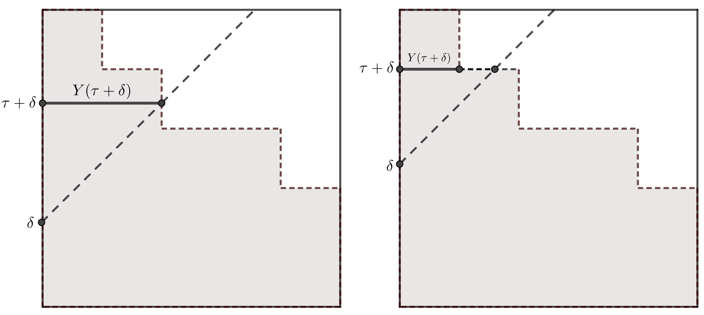
Let us now consider the following linear function of vv

f⁡(v)=v−δf(v)=v-\delta

and let τ\tau be such, that τ+δ\tau+\delta is an argument at which the graph of ff and the ”staircase” part of bd⁡(A)\mathrm{bd}(A) intersect - see Figure  5.

Refer to caption
Figure 5: graph of ff intersects either horizontal or vertical part of the ”staircase”

Clearly, we have two possible scenarios. Firstly, graph of ff may intersect vertical part of the boundary. In this case, let us note that

y​(τ+δ)=f⁡(τ+δ)=(τ+δ)−δ=τ.\textbf{y}(\tau+\delta)\ =\ f(\tau+\delta)\ =\ (\tau+\delta)-\delta\ =\ \tau.

On the other hand, assume that ff intersects horizontal part of the ”staircase”. Having this in mind, recall that we have omitted bd⁡(A)\mathrm{bd}(A) in the construction of (X,Y)(X,Y). This leaves us with

y​(τ+δ)=λ⁡((A∖bd⁡(A))∩([0,1]×(τ+δ)))≤f⁡(τ+δ)=τ.\textbf{y}(\tau+\delta)\ =\ \lambda\Bigg(\Big(A\setminus\mathrm{bd}(A)\Big)\cap\Big([0,1]\times(\tau+\delta)\Big)\Bigg)\ \leq\ f(\tau+\delta)\ =\ \tau.

Thus, either way, we get y​(τ+δ)≤τ\textbf{y}(\tau+\delta)\leq\tau. Again, from construction of (X,Y)(X,Y) and omission of boundary, we have

ℙ[X>(τ+δ)]=y(τ+δ)≤τ.\mathbb{P}[X>(\tau+\delta)]\ =\ \textbf{y}(\tau+\delta)\ \leq\ \tau.

Hence, it remains to check, that

ℙ[Y<τ]≤ 1−τ−δ,\mathbb{P}[Y<\tau]\ \leq\ 1-\tau-\delta,

or equivalently, that

ℙ[Y≥τ]≥τ+δ.\mathbb{P}[Y\geq\tau]\ \geq\ \tau+\delta.

Luckily, observe that

ℙ[Y≥τ]=ℙ[y(V)≥τ],\mathbb{P}[Y\geq\tau]\ =\ \mathbb{P}[\textbf{y}(V)\geq\tau],

and y​(v)≥τ\textbf{y}(v)\geq\tau for all v<τ+δv<\tau+\delta. □\square

5 Upper bounds and a novel approach

We will continue exploiting combinatorial nature of Ferrer diagrams. We shall start by introducing more flexible definitions.

5.1 Generalization of Ferrer diagrams

Definition 5.1.

From now on, by (generalised) Ferrer diagram, we shall mean a set

Ff={(u,v)∈[0,1]2:v<f⁡(u)},F_{f}\ =\ \{(u,v)\in[0,1]^{2}\ :\ v<f(u)\},

where

f:[0,1]→[0,1],f:[0,1]\rightarrow[0,1],

is any weakly decreasing step function that takes finitely many differernt values; let us denote the set of such step functions as 𝕊​𝕋​𝔼​ℙ.\mathbb{STEP}.

In the next definition, we formalise an idea used in the proof of Theorem 4.4 - compare Figure  4.

Definition 5.2.

For any Ferrer diagram FfF_{f} we define a pair of associated random variables

(Xf,Yf)∈𝒞ℐdefined on a probability space(I,ℒλ⊗λ​(I),λ⊗λ),(X_{f},Y_{f})\in\mathcal{C}_{\mathcal{I}}\ \ \ \ \text{defined on a probability space}\ \ \ \Big(I,\mathcal{L}_{\lambda\otimes\lambda}(I),\lambda\otimes\lambda\Big),

where I={(u,v):u,v∈[0,1]}I=\Big\{(u,v):u,v\in[0,1]\Big\}, by

Xf​(u,v)≡xf​(U⁡(u,v)):=λ⁡((Ff∖bd⁡(Ff))∩(u×[0,1])),X_{f}(u,v)\ \equiv\ \textbf{x}_{f}(U(u,v))\ :=\ \lambda\Bigg(\Big(F_{f}\setminus\mathrm{bd}(F_{f})\Big)\cap\Big(u\times[0,1]\Big)\Bigg), (8)
Yf​(u,v)≡yf​(V⁡(u,v)):=λ⁡((Ff∖bd⁡(Ff))∩([0,1]×v)),Y_{f}(u,v)\ \equiv\ \textbf{y}_{f}(V(u,v))\ :=\ \lambda\Bigg(\Big(F_{f}\setminus\mathrm{bd}(F_{f})\Big)\cap\Big([0,1]\times v\Big)\Bigg), (9)

where

U⁡(u,v)=u,U(u,v)=u,
V⁡(u,v)=v.V(u,v)=v.

We shall prove that (Xf,Yf)(X_{f},Y_{f}) defined by (8) and (9) does satisfy (Xf,Yf)∈𝒞ℐ(X_{f},Y_{f})\in\mathcal{C}_{\mathcal{I}}.

Proof: Clearly U,V∼𝒰⁡[0,1]U,V\sim\mathcal{U}[0,1] and U⟂VU\perp V. This gives X⟂YX\perp Y. It is therefore enough to check that

Xf​(u,v)≡xf​(U⁡(u,v))=𝔼⁡(𝟙Ff∖bd⁡(Ff)|U=u),X_{f}(u,v)\ \equiv\ \textbf{x}_{f}(U(u,v))\ \ =\ \ \mathbb{E}(\mathds{1}_{F_{f}\setminus\mathrm{bd}(F_{f})}|U=u), (10)
Yf​(u,v)≡yf​(V⁡(u,v))=𝔼⁡(𝟙Ff∖bd⁡(Ff)|V=v).Y_{f}(u,v)\ \equiv\ \textbf{y}_{f}(V(u,v))\ \ =\ \ \mathbb{E}(\mathds{1}_{F_{f}\setminus\mathrm{bd}(F_{f})}|V=v). (11)

This gives (Xf,Yf)∈𝒞(X_{f},Y_{f})\in\mathcal{C}. We limit ourselves to showing (10). It is straightforward to check that xf\textbf{x}_{f} is a borel function. Thus by (8) we have

Xf=xf​(U),X_{f}=\textbf{x}_{f}(U),

and XfX_{f} is σ⁡(U)\sigma(U) measurable. It remains to verify that for every A∈σ⁡(U)A\in\sigma(U), we have

∫AXf​𝑑ℙ=∫A𝟙Ff∖bd⁡(Ff)​𝑑ℙ.\int_{A}X_{f}\ \mathrm{d}\mathbb{P}\ =\ \int_{A}\mathds{1}_{F_{f}\setminus\mathrm{bd}(F_{f})}\ \mathrm{d}\mathbb{P}.

The condition A∈σ⁡(U)A\in\sigma(U) is equivalent to A=A~×[0,1]A=\tilde{A}\times[0,1], for some A~∈ℒ⁡([0,1])\tilde{A}\in\mathcal{L}([0,1]). We can write

xf​(u)=λ⁡((Ff∖bd⁡(Ff))∩(u×[0,1]))=∫01𝟙Ff∖bd⁡(Ff)​(u,v)​𝑑λ​(v),\textbf{x}_{f}(u)\ =\ \lambda\Bigg(\Big(F_{f}\setminus\mathrm{bd}(F_{f})\Big)\cap\Big(u\times[0,1]\Big)\Bigg)\ =\ \int_{0}^{1}\mathds{1}_{F_{f}\setminus\mathrm{bd}(F_{f})}(u,v)\ \mathrm{d}\lambda(v),

and hence, by Fubini’s theorem, we have

∫A𝟙Ff∖bd⁡(Ff)​𝑑ℙ=∫A~[∫[0,1]𝟙Ff∖bd⁡(Ff)​(u,v)​𝑑λ​(v)]​𝑑λ​(u)\int_{A}\mathds{1}_{F_{f}\setminus\mathrm{bd}(F_{f})}\ \mathrm{d}\mathbb{P}\ =\ \int_{\tilde{A}}\Bigg[\int_{[0,1]}\mathds{1}_{F_{f}\setminus\mathrm{bd}(F_{f})}(u,v)\ \mathrm{d}\lambda(v)\Bigg]\mathrm{d}\lambda(u)
=∫A~xf(u)dλ(u)=∫AXf(u,v)dλ2(u,v)=∫AXfdℙ,=\ \int_{\tilde{A}}\textbf{x}_{f}(u)\ \mathrm{d}\lambda(u)\ =\ \int_{A}X_{f}(u,v)\ \mathrm{d}\lambda_{2}(u,v)\ \ =\ \ \int_{A}X_{f}\ \mathrm{d}\mathbb{P},

as required. □\square

Although it is rather obvious, let us state the following

Proposition 5.1.

For all k∈ℤ+k\in\mathbb{Z}_{+}, k≥3k\geq 3, we simply have

supf∈𝕊​𝕋​𝔼​ℙ𝔼​|Xf−Yf|k=sup(X,Y)∈𝒞ℐ𝔼​|X−Y|k.\sup_{f\ \in\ \mathbb{STEP}}\ \mathbb{E}|X_{f}-Y_{f}|^{k}\ =\ \sup_{(X,Y)\in\mathcal{C}_{\mathcal{I}}}\mathbb{E}|X-Y|^{k}.

Proof: For all f∈𝕊​𝕋​𝔼​ℙf\in\mathbb{STEP}, by definition

(Xf,Yf)∈𝒞ℐ,(X_{f},Y_{f})\ \in\mathcal{C}_{\mathcal{I}},

and thus, the inequality

supf∈𝕊​𝕋​𝔼​ℙ𝔼​|Xf−Yf|k≤sup(X,Y)∈𝒞ℐ𝔼​|X−Y|k,\sup_{f\ \in\ \mathbb{STEP}}\ \mathbb{E}|X_{f}-Y_{f}|^{k}\ \leq\ \sup_{(X,Y)\in\mathcal{C}_{\mathcal{I}}}\mathbb{E}|X-Y|^{k},

is clear. The opposite inequality follows from the same argument as the proof of Theorem 4.4. □\square

5.2 Sharpening a layer-cake upper bound

In this section we will continue our analysis of upper bounds generated by the layer-cake representation (5). Let us start with a brief overview of the relevant results. As already mentioned, in [2] it was proved that for δ∈(12,1],\delta\in(\frac{1}{2},1], we have

sup(X,Y)∈𝒞ℙ⁡(|X−Y|≥δ)≤ 2​(1−δ).\sup_{(X,Y)\in\mathcal{C}}\mathbb{P}(|X-Y|\geq\delta)\ \leq\ 2(1-\delta).

This result has been lately greatly improved by Burdzy and Pal. In [3] they proved that for δ∈(12,1]\delta\in(\frac{1}{2},1]:

sup(X,Y)∈𝒞ℙ⁡(|X−Y|≥δ)=2​(1−δ)2−δ.\sup_{(X,Y)\in\mathcal{C}}\mathbb{P}(|X-Y|\geq\delta)\ =\ \frac{2(1-\delta)}{2-\delta}.

Moreover, for all δ\delta in this range, one can find such pairs (Xδ,Yδ)∈𝒞(X_{\delta},Y_{\delta})\in\mathcal{C} for which the equality is attained. It is however important to note that for δ<1\delta<1, those variables turn out to be dependent. It is relatively easy to check that for δ∈(12,1]\delta\in(\frac{1}{2},1]:

sup(X,Y)∈𝒞ℐ​(2)ℙ⁡(|X−Y|≥δ)= 2​δ​(1−δ).\sup_{(X,Y)\in\mathcal{C}_{\mathcal{I}}(2)}\mathbb{P}(|X-Y|\geq\delta)\ =\ 2\delta(1-\delta).

Based on this premise, Burdzy and Pitman conjectured in [1], that for δ∈(12,1]\delta\in(\frac{1}{2},1], we have

sup(X,Y)∈𝒞ℐℙ⁡(|X−Y|≥δ)= 2​δ​(1−δ).\sup_{(X,Y)\in\mathcal{C}_{\mathcal{I}}}\mathbb{P}(|X-Y|\geq\delta)\ =\ 2\delta(1-\delta). (12)

In this chapter we will prove a result, that is strikingly similar. Namely, for δ∈(12,1]\delta\in(\frac{1}{2},1], we have

supf∈𝕊​𝕋​𝔼​ℙℙ⁡(|Xf−Yf|>δ)= 2​δ​(1−δ).\sup_{f\ \in\ \mathbb{STEP}}\mathbb{P}(|X_{f}-Y_{f}|>\delta)\ =\ 2\delta(1-\delta). (13)

In this place let us highlight that, thanks to Proposition 5.1, both (12) and (13) generate exactly the same layer-cake bound on

sup(X,Y)∈𝒞ℐ𝔼​|X−Y|k,\sup_{(X,Y)\in\mathcal{C}_{\mathcal{I}}}\mathbb{E}|X-Y|^{k},

for all k∈ℤ+,k≥3.k\in\mathbb{Z}_{+},k\geq 3. We begin with the simple, but useful observation.

Refer to caption
Figure 6: either (xf​(s)≤t)∧(yf​(t)≤s)(\textbf{x}_{f}(s)\leq t)\ \wedge\ (\textbf{y}_{f}(t)\leq s) or (xf​(s)≥t)∧(yf​(t)≥s)(\textbf{x}_{f}(s)\geq t)\ \wedge\ (\textbf{y}_{f}(t)\geq s).
Lemma 5.1.

Fix f∈𝕊​𝕋​𝔼​ℙf\in\mathbb{STEP} and consider the associated (Xf,Yf)∈𝒞ℐ(X_{f},Y_{f})\in\mathcal{C}_{\mathcal{I}}. For any s,t∈[0,1]s,t\in[0,1], there are only two possible scenarios:

either{xf​(s)≤t,yf​(t)≤s,or{xf​(s)≥t,yf​(t)≥s.\text{either}\ \ \ \ \left\{\begin{array}[]{ll}\textbf{x}_{f}(s)\ \leq\ t,\\ \textbf{y}_{f}(t)\ \leq\ s,\end{array}\right.\ \ \ \ \ \text{or}\ \ \ \ \ \left\{\begin{array}[]{ll}\textbf{x}_{f}(s)\ \geq\ t,\\ \textbf{y}_{f}(t)\ \geq\ s.\end{array}\right.

Proof: This is a direct consequence of the definitions - see Figure  6. □\square

Theorem 5.1.

For all δ∈(12,1]\delta\in(\frac{1}{2},1], we have

supf∈𝕊​𝕋​𝔼​ℙℙ⁡(|Xf−Yf|>δ)= 2​δ​(1−δ).\sup_{f\ \in\ \mathbb{STEP}}\mathbb{P}(|X_{f}-Y_{f}|>\delta)\ =\ 2\delta(1-\delta).

Proof of this theorem will be based on two lemmas, which follow below.

Lemma 5.2.

Fix δ∈(12,1]\delta\in(\frac{1}{2},1] and consider any f∈𝕊​𝕋​𝔼​ℙf\in\mathbb{STEP}, for which one of conditions:

{xf​(δ)≥δ,yf​(δ)≥δ,\left\{\begin{array}[]{ll}\textbf{x}_{f}(\delta)\ \geq\ \delta,\\ \textbf{y}_{f}(\delta)\ \geq\ \delta,\end{array}\right. (14)

or

{xf​(1−δ)≤ 1−δ,yf​(1−δ)≤ 1−δ,\left\{\begin{array}[]{ll}\textbf{x}_{f}(1-\delta)\ \leq\ 1-\delta,\\ \textbf{y}_{f}(1-\delta)\ \leq\ 1-\delta,\end{array}\right. (15)

is satisfied. Then we have

ℙ⁡(|Xf−Yf|>δ)≤ 2​δ​(1−δ).\mathbb{P}(|X_{f}-Y_{f}|>\delta)\ \leq\ 2\delta(1-\delta).

Proof: Let us first consider point (14). We start by writing

ℙ(|Xf−Yf|>δ)=ℙ[Xf>(Yf+δ)]+ℙ[Yf>(Xf+δ)].\mathbb{P}(|X_{f}-Y_{f}|>\delta)\ =\ \mathbb{P}[X_{f}>(Y_{f}+\delta)]\ +\ \mathbb{P}[Y_{f}>(X_{f}+\delta)].

By independence, we can evaluate

ℙ[Xf>(Yf+δ)]≤ℙ[Xf>δ]⋅ℙ[Yf≤δ]=yf(δ)(1−xf(δ)).\mathbb{P}[X_{f}>(Y_{f}+\delta)]\ \leq\ \mathbb{P}[X_{f}>\delta]\cdot\mathbb{P}[Y_{f}\leq\delta]\ =\ \textbf{y}_{f}(\delta)(1-\textbf{x}_{f}(\delta)).
ℙ[Yf>(Xf+δ)]≤ℙ[Yf>δ]⋅ℙ[Xf≤δ]=xf(δ)(1−yf(δ)).\mathbb{P}[Y_{f}>(X_{f}+\delta)]\ \leq\ \mathbb{P}[Y_{f}>\delta]\cdot\mathbb{P}[X_{f}\leq\delta]\ =\ \textbf{x}_{f}(\delta)(1-\textbf{y}_{f}(\delta)).

Summing up, we get

ℙ⁡(|Xf−Yf|>δ)≤yf​(δ)​(1−xf​(δ))+xf​(δ)​(1−yf​(δ))\mathbb{P}(|X_{f}-Y_{f}|>\delta)\ \ \ \leq\ \ \ \textbf{y}_{f}(\delta)(1-\textbf{x}_{f}(\delta))\ +\ \textbf{x}_{f}(\delta)(1-\textbf{y}_{f}(\delta))
≤supx,y∈[δ,1]g⁡(x,y),\ \ \ \leq\ \ \ \sup_{x,y\ \in\ [\delta,1]}g(x,y),

where g⁡(x,y)=y⁡(1−x)+x⁡(1−y).g(x,y)=y(1-x)+x(1-y). Since δ>12,\delta>\frac{1}{2}, we get

∂g∂x​(x,y)= 1−2​y< 0,\frac{\partial g}{\partial x}(x,y)\ =\ 1-2y\ <\ 0,
∂g∂y​(x,y)= 1−2​x< 0,\frac{\partial g}{\partial y}(x,y)\ =\ 1-2x\ <\ 0,

and hence

ℙ⁡(|Xf−Yf|>δ)≤g⁡(δ,δ)=2​δ​(1−δ),\mathbb{P}(|X_{f}-Y_{f}|>\delta)\ \leq\ g(\delta,\delta)=2\delta(1-\delta),

which was to be proved.

The proof of point (15) is similar and we will only sketch it. One can evaluate

ℙ(|Xf−Yf|>δ)≤ℙ[Xf>1−δ]⋅ℙ[Yf≤1−δ]+ℙ[Yf>1−δ]⋅ℙ[Xf≤1−δ]\mathbb{P}(|X_{f}-Y_{f}|>\delta)\ \leq\ \mathbb{P}[X_{f}>1-\delta]\cdot\mathbb{P}[Y_{f}\leq 1-\delta]\ +\ \mathbb{P}[Y_{f}>1-\delta]\cdot\mathbb{P}[X_{f}\leq 1-\delta]
=yf​(1−δ)​(1−xf​(1−δ))+xf​(1−δ)​(1−yf​(1−δ))=\ \textbf{y}_{f}(1-\delta)(1-\textbf{x}_{f}(1-\delta))\ +\ \textbf{x}_{f}(1-\delta)(1-\textbf{y}_{f}(1-\delta))
≤supx,y∈[0,1−δ]g⁡(x,y)= 2​δ​(1−δ),\leq\ \sup_{x,y\ \in\ [0,1-\delta]}g(x,y)\ =\ 2\delta(1-\delta),

where the last line is a consequence of 1−δ<121-\delta<\frac{1}{2}. □\square

Lemma 5.3.

For all δ∈(12,1]\delta\in(\frac{1}{2},1] and any f∈𝕊​𝕋​𝔼​ℙf\in\mathbb{STEP}, if

1−δ≤yf​(δ)≤δ,1-\delta\ \leq\ \textbf{y}_{f}(\delta)\ \leq\ \delta,

then

ℙ⁡(Xf>Yf+δ)≤δ⁡(1−δ).\mathbb{P}(X_{f}>Y_{f}+\delta)\ \leq\ \delta(1-\delta).

The same holds true for XfX_{f} and YfY_{f} with switched roles.

Proof: Just as previously, due to independence, we can write

ℙ(Xf>Yf+δ)≤ℙ[Xf>δ]⋅ℙ[Yf<1−δ].\mathbb{P}(X_{f}>Y_{f}+\delta)\ \leq\ \mathbb{P}[X_{f}>\delta]\cdot\mathbb{P}[Y_{f}<1-\delta].

Firstly, note that

ℙ[Xf>δ]=yf(δ)≤δ.\mathbb{P}[X_{f}>\delta]\ =\ \textbf{y}_{f}(\delta)\ \leq\ \delta.

Secondly, thanks to monotonicity of YfY_{f}, we have

yf​(ω)≥yf​(δ)≥ 1−δfor allω≤δ,\textbf{y}_{f}(\omega)\ \geq\ \textbf{y}_{f}(\delta)\ \geq\ 1-\delta\ \ \ \ \ \ \ \text{for all}\ \ \ \ \ \ \ \omega\ \leq\ \delta,

so {yf<1−δ}⊂(δ,1],\{\textbf{y}_{f}<1-\delta\}\subset(\delta,1], and hence

ℙ[Yf<1−δ]≤ 1−δ,\mathbb{P}[Y_{f}<1-\delta]\ \leq\ 1-\delta,

which completes the proof. □\square

Proof of Theorem 5.1: Fix δ∈(12,1]\delta\in(\frac{1}{2},1] and any f∈𝕊​𝕋​𝔼​ℙf\in\mathbb{STEP}. It is enough to check, that

ℙ⁡(|Xf−Yf|>δ)≤ 2​δ​(1−δ).\mathbb{P}(|X_{f}-Y_{f}|>\delta)\ \leq\ 2\delta(1-\delta).

By Lemmas 5.1 and 5.2 (14), we can assume, that

{xf​(δ)≤δ,yf​(δ)≤δ.\left\{\begin{array}[]{ll}\textbf{x}_{f}(\delta)\ \leq\ \delta,\\ \textbf{y}_{f}(\delta)\ \leq\ \delta.\end{array}\right. (16)

By the Lemma 5.1 again, there are only 44 possible scenarios:

{xf​(1−δ)≥δ,yf​(δ)≥ 1−δ,and{yf​(1−δ)≥δ,xf​(δ)≥ 1−δ.\left\{\begin{array}[]{ll}\textbf{x}_{f}(1-\delta)\ \geq\ \delta,\\ \textbf{y}_{f}(\delta)\ \geq\ 1-\delta,\end{array}\right.\ \ \ \text{and}\ \ \ \left\{\begin{array}[]{ll}\textbf{y}_{f}(1-\delta)\ \geq\ \delta,\\ \textbf{x}_{f}(\delta)\ \geq\ 1-\delta.\end{array}\right. (17)
{xf​(1−δ)≥δ,yf​(δ)≥ 1−δ,and{yf​(1−δ)≤δ,xf​(δ)≤ 1−δ.\left\{\begin{array}[]{ll}\textbf{x}_{f}(1-\delta)\ \geq\ \delta,\\ \textbf{y}_{f}(\delta)\ \geq\ 1-\delta,\end{array}\right.\ \ \ \text{and}\ \ \ \left\{\begin{array}[]{ll}\textbf{y}_{f}(1-\delta)\ \leq\ \delta,\\ \textbf{x}_{f}(\delta)\ \leq\ 1-\delta.\end{array}\right. (18)
{xf​(1−δ)≤δ,yf​(δ)≤ 1−δ,and{yf​(1−δ)≥δ,xf​(δ)≥ 1−δ.\left\{\begin{array}[]{ll}\textbf{x}_{f}(1-\delta)\ \leq\ \delta,\\ \textbf{y}_{f}(\delta)\ \leq\ 1-\delta,\end{array}\right.\ \ \ \text{and}\ \ \ \left\{\begin{array}[]{ll}\textbf{y}_{f}(1-\delta)\ \geq\ \delta,\\ \textbf{x}_{f}(\delta)\ \geq\ 1-\delta.\end{array}\right. (19)
{xf​(1−δ)≤δ,yf​(δ)≤ 1−δ,and{yf​(1−δ)≤δ,xf​(δ)≤ 1−δ.\left\{\begin{array}[]{ll}\textbf{x}_{f}(1-\delta)\ \leq\ \delta,\\ \textbf{y}_{f}(\delta)\ \leq\ 1-\delta,\end{array}\right.\ \ \ \text{and}\ \ \ \left\{\begin{array}[]{ll}\textbf{y}_{f}(1-\delta)\ \leq\ \delta,\\ \textbf{x}_{f}(\delta)\ \leq\ 1-\delta.\end{array}\right. (20)

We continue by inspection, one by one.

(17). In view of (16) we have

1−δ≤yf​(δ)≤δ,1-\delta\ \leq\ \textbf{y}_{f}(\delta)\ \leq\ \delta,
1−δ≤xf​(δ)≤δ.1-\delta\ \leq\ \textbf{x}_{f}(\delta)\ \leq\ \delta.

By a double use of Lemma 5.3, we get

ℙ(|Xf−Yf|>δ)=ℙ[Xf>(Yf+δ)]+ℙ[Yf>(Xf+δ)]\mathbb{P}(|X_{f}-Y_{f}|>\delta)\ =\ \mathbb{P}[X_{f}>(Y_{f}+\delta)]\ +\ \mathbb{P}[Y_{f}>(X_{f}+\delta)]
≤δ⁡(1−δ)+δ⁡(1−δ)= 2​δ​(1−δ).△\leq\ \delta(1-\delta)\ +\ \delta(1-\delta)\ =\ 2\delta(1-\delta).\ \ \ \ \triangle

(18). In view of (16) we have

1−δ≤yf​(δ)≤δ.1-\delta\ \leq\ \textbf{y}_{f}(\delta)\ \leq\ \delta.

From Lemma 5.3, we have

ℙ[Xf>Yf+δ]≤δ(1−δ).\mathbb{P}[X_{f}>Y_{f}+\delta]\ \leq\ \delta(1-\delta).

Furthermore, since to δ∈(12,1]\delta\in(\frac{1}{2},1], we can evaluate

ℙ[Yf>Xf+δ]≤ℙ(Yf>δ)⋅ℙ(Xf<δ).\mathbb{P}[Y_{f}>X_{f}+\delta]\ \leq\ \mathbb{P}(Y_{f}>\delta)\cdot\mathbb{P}(X_{f}<\delta).

By monotonicity, we have

yf​(v)≤yf​(1−δ)≤δfor allv≥ 1−δ,\textbf{y}_{f}(v)\ \leq\ \textbf{y}_{f}(1-\delta)\ \leq\ \delta\ \ \ \ \ \ \ \text{for all}\ \ \ \ \ \ \ v\ \geq\ 1-\delta,
xf​(u)≥xf​(1−δ)≥δfor allu≤ 1−δ,\textbf{x}_{f}(u)\ \geq\ \textbf{x}_{f}(1-\delta)\ \geq\ \delta\ \ \ \ \ \ \ \text{for all}\ \ \ \ \ \ \ u\ \leq\ 1-\delta,

so

{yf>δ}⊂[0,1−δ),\{\textbf{y}_{f}>\delta\}\ \subset\ [0,1-\delta),
{xf<δ}⊂(1−δ,1],\{\textbf{x}_{f}<\delta\}\ \subset\ (1-\delta,1],

and hence

ℙ[Yf>Xf+δ]≤(1−δ)δ.△\mathbb{P}[Y_{f}>X_{f}+\delta]\ \leq\ (1-\delta)\delta.\ \ \ \ \triangle


(19). This scenario is analogous to (18). It is sufficient to change roles of XfX_{f} and YfY_{f}. △\triangle

(20). Let us start by repeating again the bounds for this scenario. We have

{xf​(1−δ)≤δ,xf​(δ)≤ 1−δ,and{yf​(1−δ)≤δ,yf​(δ)≤ 1−δ.\left\{\begin{array}[]{ll}\textbf{x}_{f}(1-\delta)\ \leq\ \delta,\\ \textbf{x}_{f}(\delta)\ \leq\ 1-\delta,\end{array}\right.\ \ \ \text{and}\ \ \ \left\{\begin{array}[]{ll}\textbf{y}_{f}(1-\delta)\ \leq\ \delta,\\ \textbf{y}_{f}(\delta)\ \leq\ 1-\delta.\end{array}\right.

At this point, it is beneficial to graph the constraints given by (20).

Refer to caption
Figure 7: example diagram FfF_{f} meeting constraints given by (20).

As in Figure  7; every diagram FfF_{f} meeting constraints discussed in scenario (20), must be a subset of hatched region. For any such diagram FfF_{f}, let us now define

Ff′=Ff∖[1−δ,δ]2.F_{f^{\prime}}=F_{f}\setminus[1-\delta,\delta]^{2}.

Put differently, we are removing the (possibly empty) interesection Ff∩[1−δ,δ]2F_{f}\cap[1-\delta,\delta]^{2} - see Figure  8.

Refer to caption
Figure 8: diagram Ff′F_{f^{\prime}} is obtained from FfF_{f} by removing [1−δ,δ]2[1-\delta,\delta]^{2} .

Note that, by construction, the transformation Ff→Ff′F_{f}\to F_{f^{\prime}} fulfils both

xf′≤xf,\textbf{x}_{f^{\prime}}\ \leq\ \textbf{x}_{f},
yf′≤yf,\textbf{y}_{f^{\prime}}\ \leq\ \textbf{y}_{f},

and

xf′​(u)=xf​(u)for allu∈{u:xf​(u)>δ},\textbf{x}_{f^{\prime}}(u)\ =\ \textbf{x}_{f}(u)\ \ \ \ \ \ \ \text{for all}\ \ \ \ \ \ \ u\ \in\ \{u:\textbf{x}_{f}(u)>\delta\},
yf′​(v)=yf​(v)for allv∈{v:yf​(v)>δ}.\textbf{y}_{f^{\prime}}(v)\ =\ \textbf{y}_{f}(v)\ \ \ \ \ \ \ \text{for all}\ \ \ \ \ \ \ v\ \in\ \{v:\textbf{y}_{f}(v)>\delta\}.

Thus, it is straightforward to see, that

ℙ⁡(Xf>Yf+δ)≤ℙ⁡(Xf′>Yf′+δ),\mathbb{P}(X_{f}>Y_{f}+\delta)\ \leq\ \mathbb{P}(X_{f^{\prime}}>Y_{f^{\prime}}+\delta),
ℙ⁡(Yf>Xf+δ)≤ℙ⁡(Yf′>Xf′+δ),\mathbb{P}(Y_{f}>X_{f}+\delta)\ \leq\ \mathbb{P}(Y_{f^{\prime}}>X_{f^{\prime}}+\delta),

and

ℙ⁡(|Xf−Yf|>δ)≤ℙ⁡(|Xf′−Yf′|>δ),\mathbb{P}(|X_{f}-Y_{f}|>\delta)\ \leq\ \mathbb{P}(|X_{f^{\prime}}-Y_{f^{\prime}}|>\delta),

as a result. To complete the proof, it is enough to show, that

ℙ⁡(|Xf′−Yf′|>δ)≤ 2​δ​(1−δ),\mathbb{P}(|X_{f^{\prime}}-Y_{f^{\prime}}|>\delta)\ \leq\ 2\delta(1-\delta),

but this is a direct consequence of Lemma 5.2 (15). △\triangle □\square

By Proposition 5.1 and Theorem 5.1, we get the following corollary directly.

Corollary 5.1.

For all k∈ℤ+k\in\mathbb{Z}_{+}, k≥3k\geq 3, we have

sup(X,Y)∈𝒞ℐ𝔼​|X−Y|k≤∫012k​tk−1​𝑑t+∫121k​tk−1⋅2​t​(1−t)​𝑑t,\sup_{(X,Y)\in\mathcal{C}_{\mathcal{I}}}\mathbb{E}|X-Y|^{k}\ \leq\ \int_{0}^{\frac{1}{2}}kt^{k-1}\mathrm{d}t\ +\ \int_{\frac{1}{2}}^{1}kt^{k-1}\cdot 2t(1-t)\mathrm{d}{t},

that is

sup(X,Y)∈𝒞ℐ𝔼​|X−Y|k≤ 2⋅k(k+1)​(k+2)+ 2−k− 2−k−1⋅k⁡(k+3)(k+1)​(k+2).\sup_{(X,Y)\in\mathcal{C}_{\mathcal{I}}}\mathbb{E}|X-Y|^{k}\ \leq\ 2\cdot\frac{k}{(k+1)(k+2)}+\ 2^{-k}\ -\ 2^{-k-1}\cdot\frac{k(k+3)}{(k+1)(k+2)}.

References

  • [1]
  • [1] Krzysztof Burdzy, Jim Pitman, Bounds on the probability of radically different opinions, arXiv:1903.07773 [math.PR], (2019)
  • [2] Krzysztof Burdzy, Resonance: From Probability to Epistemology and Back, Imperial College Press, (2016)
  • [3] Krzysztof Burdzy, Soumik Pal, Contradictory Predictions, arXiv:1912.00126 [math.PR], (2019)
  • [4] A. R. Dawid, M. H. DeGroot, J. Mortera, Coherent combination of experts’ opinions , Test 4, 263–313, (1995)
  • [5] Lester E. Dubins, Jim Pitman, A maximal inequality for skew fields, Zeitschrift für Wahrscheinlichkeitstheorie und Verwandte Gebiete 52, 219–22, (1980)
  • [6] Jessica N. Copher, Sums of Squared Distances between Points on a Unit n-Sphere, arXiv:2001.02745v1 [math.MG], (2020)
  • [7] Bojana Borovicanin , Kinkar Ch. Das, Boris Furtula , Ivan Gutman, Bounds for Zagreb Indices, MATCH Commun. Math. Comput. Chem. 78, (2017)
  • [8] Jeffrey W. Miller, Reduced Criteria for Degree Sequences, arXiv:1205.2686 [math.CO], (2013)
  • [9] N.V.R. Mahadev, U.N. Peled, Threshold Graphs and Related Topics, Elsevier Science Publisher B.V., (1995)
  • [10] Tamás Réti, Akbar Ali, Some Generalizations of the Total Irregularity of Graphs, Scientific Publications of the State University of Novi Pazar Series A: Applied Mathematics, Informatics and mechanics, vol. 11.1, 1-9, (2019)
  • [11] Lev Kourliandtchik, Wędrówki po krainie nierówności, Wydawnictwo Aksjomat, (2006)
  • [12] J. Jakubowski, R. Sztencel, Wstęp do teorii prawdopodobieństwa, Wydawnictwo SCRIPT, (2010)
  • [13] Kenneth A. Ross, Charles R. B. Wright, Matematyka dyskretna, Wydawnictwo Naukowe PWN, (2012)