A Fast Iterative Algorithm to design phase only sequences by minimizing the ISL metric
Abstract
Unimodular/Phase only sequence having impulse like aperiodic auto-correlation function plays a central role in the applications of RADAR, SONAR, Cryptography, and Wireless (CDMA) Communication Systems. In this paper, we propose a fast iterative algorithm to design phase only sequences of arbitrary lengths by minimizing the Integrated Side-lobe Level (ISL) metric, which is very closely related to the auto-correlation property of a sequence. The ISL minimization problem is solved iteratively by using the Majorization-Minimization (MM) technique, which ensures a monotonic convergence to the stationary minimum point. To highlight the performance of a proposed algorithm, we conduct the numerical experiments for different sequence lengths using different initializations and also compare them with the existing algorithms. Numerical simulations show that irrespective of the sequence length and initialization, the proposed algorithm is performing better than the state-of-the-art algorithms in terms of speed of convergence. We also show a computationally efficient way to implement our proposed algorithm by using the FFT and IFFT operations.
Index Terms– Majorization-Minimization, Integrated Side-lobe Level, Peak Side-lobe Level, Phase only sequence, aperiodic auto-correlation, Cryptography, Communication Systems, RADAR, SONAR, MIMO RADAR, CDMA.
I.INTRODUCTION
The target detection capability of an active sensing system will solely depend on the accuracy of the estimated underlying parameters. So, to increase the detection performance in applications like active sensing systems (SONAR, RADAR) [1], [2], [3], [4], [5], Cryptography [6], CDMA communication systems [7], [8], [9], and MIMO RADAR [10-17], finite-length transmit sequences with impulse like aperiodic auto-correlation function is a necessity. However, in real life, along with good correlation property, the aforementioned applications also pose different constraints on the transmit sequence like the power and spectral (range of operating frequencies) constraints. The power constraint is mainly due to the limited budget of transmitter power available in the system. Hence, the design of phase only sequences of arbitrary lengths having unit magnitude and impulse like aperiodic auto-correlation function is always desired [18], [19], [7].
Earlier, design of phase only sequences is done mainly by algebraic approaches and some of the sequences designed through algebraic approaches are Barker sequence [20], [21], Frank sequence [22], Golomb sequence [23], Chu sequence [23], [3] and P4 sequence [24], [25]. But all the above-mentioned sequences exist only for the shorter lengths and have limited degrees of freedom. Hence, algebraic approaches are not viable to generate sequences of large lengths. To overcome this issue, recently, computational approaches [7], [26], [27], [28], came into existence and enabled a way to design sequences of arbitrary lengths at a slighter computational cost. Some of the developed computational approaches are the stochastic search methods [29], exhaustive search methods [30], which are heuristic in nature with no guarantee for convergence to a stationary point of ISL function. To overcome all such issues, very recently several optimization methods [31], [8], [4], [32] came into the existence and some of the approaches are CAN [33], MISL [34], ISL-NEW [35], MM-Corr [36], ADMM approach [37], MWISL, MWISL-Diag, MM-PSL [38], and CPM [39]- a detailed review of some of the methods will follow shortly. The following mathematical notations are used hereafter: boldface lowercase letters denote column vectors, boldface uppercase letters denote matrices and italics denote scalars. The superscripts denote complex conjugate, transpose, and conjugate transpose, respectively. denote the trace of a matrix. denote the element of a vector . and denote the real and imaginary parts, respectively. denote the identity matrix. denote the norm. is a column vector that consists of all the columns of a matrix- stacked. denote the absolute squared value. is a diagonal matrix formed with a vector as its diagonal. and represent the real and complex fields. denote the maximum eigenvalue of . denote the gradient of a function represents the first elements of a vector .
A. SIGNAL MODEL AND PROBLEM FORMULATION
Let be a phase only sequence of length to be designed. The element of a sequence is denoted as , where is an arbitrary phase angle that varies between and radians. The aperiodic auto-correlation function of a sequence at any lag is defined as:
| (1) |
The Integrated Side-lobe Level (ISL) metric, which is a direct measure of the designed sequence is defined as:
| (2) |
The Peak Side-lobe Level (PSL) metric is defined as:
| (3) |
So, the problem to design a phase only sequence that minimizes the ISL metric is formulated as:
| (4) | ||||||
where .
Apart from the unimodular constraint, there are interests in imposing constraints like binary constraint [28], [26], [40], spectral constraint [41], [42], [43], similarity constraint [44], [45], Peak to Average Power Ratio (PAPR) constraint [46] to name a few.
In the next subsection, we will discuss the general framework of majorization-minimization, which would play a central role in the development of our algorithm.
B. Majorization-Minimization Method
Majorization-Minimization (MM) is a two-step technique, which is used to solve the hard (non-convex or even convex) problems very efficiently [47], [48]. The first step of the MM method is to construct a majorization (upper bound) function to the original objective function at any point ( at iteration) and then second step is to minimize the upper-bound function to generate a next update . So, at every newly generated point, the above mentioned two steps will be applied repeatedly until it reaches the optimum minimum point of an original function . For any given problem, the construction of a majorization function is not unique and for the same problem, different types of majorization functions will exist. So, the performance will depend solely on the chosen majorization function and the different ways to construct a majorization function are shown in [48], [31].
The majorization function , which is constructed in the first step of the MM method has to satisfy the following properties:
| (5) |
| (6) |
where is the set consists of all the possible values of . As the MM technique is an iterative process, it will generate the sequence of points according to the following update rule:
| (7) |
The cost function value evaluated at every point generated by (7) will satisfy the descent property, i.e.
| (8) |
C. Related work and our Contributions
The existing algorithms which are developed by solving the same ISL minimization problem (4) are CAN [33], MISL [34] , ISL-NEW [35], MM-Corr [36], ADMM approach [37], MWISL, MWISL-Diag [38], CPM [39]. In the following, we will discuss them briefly and highlight their potentials and drawbacks.
Stoica et.al proposed the CAN algorithm [33], which works on the principle of alternating minimization technique. They solved the problem by transforming the objective function in (4) to the frequency domain as:
| (9) |
where are the Fourier grid frequencies. Then the problem (4) is converted into:
| (10) | ||||||
The cost function of the problem in (10) is quartic in and it is very hard to solve further. So, instead of solving (10) directly, they solved an approximate problem, which is quadratic in as shown below:
| (11) | ||||||
where . are the auxiliary phase variables. The resulting problem can be rewritten more compactly as follows:
| (12) | ||||||
where be a matrix with , and . They solved the problem in (12) by alternatively minimizing between the variables and . For a given , minimization of (12) with respeect to is given by:
| (13) |
where ( is a FFT matrix ) and for a fixed , minimizer over would be:
| (14) |
where ( is a IFFT matrix ). The pseudocode of the CAN algorithm is summarized in Algorithm 1.
Require: sequence length
1: set , initialize
2: repeat
3:
4:
5:
6:
7:
8: until convergence
We would like to point out that, instead of solving the original problem (4), the CAN algorithm had solved an approximately equivalent problem (11). So, there is no guarantee for an obtained minimum of (11) is also a minimum of the original problem in (4).
To overcome this issue, Song et.al. proposed the MISL algorithm [34] by solving the original problem (4) directly via the MM approach. So, from (10) we have,
By expanding the cost function and ignoring the constant and multiplication terms, the above problem can be rewritten more compactly as:
| (15) | ||||||
In terms of , the problem in (15) is quartic and very hard to solve further. So, by defining and , problem in (15) can be rewritten as:
| (16) | ||||||
where . The cost function in (16) is quadratic in . So, they constructed a majorization function for it by using second-order Taylor series method [48], [31], and by neglecting the constant terms, the surrogate problem can be rewritten more compactly as:
| (17) | ||||||
where The resultant problem in (17) is quadratic in , and they have majorized the cost function in the above problem once again as mentioned above, to obtain a simple closed-form solution. After majorizing for the second time and by ignoring the constant terms, the final surrogate minimization problem becomes:
| (18) | ||||||
where and . Problem in (18) can be rewritten more compactly as:
| (19) | ||||||
where . The problem in (19) has a closed-form solution:
| (20) |
The pseudocode of the MISL algorithm is summarized in Algorithm 2.
Require: sequence length
1: set , initialize
2: repeat
3:
4:
5:
6:
7:
8: until convergence
Compared to the CAN algorithm, the MISL algorithm solves the original problem in (4). So, there is an assurance of obtaining an original optimum minimum point. But, the MISL algorithm faces a drawback of slower convergence due to twice the majorization of the original objective function. To deal with the convergence issue, they have proposed acceleration schemes to accelerate the MISL algorithm.
In [35], Y. Li et.al proposed an algorithm named ISL-NEW using the MM method to design sequence-set. By particularizing it for single sequence, we observe that the only difference between the MISL and ISL-NEW algorithms is in the way they arrive at their majorizing functions. After majorizing the objective function in (16) and removing the constant terms, the final surrogate problem they solve is given by:
| (21) | ||||||
The resultant problem in (21) is quadratic in . So, they majorized the cost function in (21) once again and arrive at the following problem:
| (22) | ||||||
where . The problem in (22) can be rewritten as:
| (23) | ||||||
where . The problem in (23) has a closed-form solution
| (24) |
The pseudocode of the ISL-NEW algorithm is summarized in Algorithm 3.
Require: sequence length
1: set , initialize
2: repeat
3:
4:
5:
6:
7:
8: until convergence
Y. Li et.al has also solved the problem (4) directly and concluded it as a fast algorithm in terms of the convergence. However, due to similarity in the update step of ISL-NEW and MISL (with very little difference), ISL-NEW also suffers from slow convergence and they have also proposed acceleration schemes to accelerate the ISL-NEW algorithm. The above mentioned three algorithms CAN, MISL and ISL-NEW can be implemented via FFT and IFFT operations. Hence, they are computationally efficient for generating sequences of large lengths.
In [36], J. Song et.al proposed an algorithm named as MM-Corr to design the sequence set using the MM method. In [37], J.Liang et.al proposed a new algorithm by solving the approximately equivalent problem to problem (4) (i.e, same as CAN algorithm) by using the ADMM method and they concluded that its performance is worse than the MISL algorithm in terms of the PSL metric value in its aperiodic autocorrelation function. In [38], J.song et.al proposed three different algorithms named MWISL, MWISL-Diag, and MM-PSL by using the MM method. We observe that out of three algorithms MWISL and MWISL-Diag are variants of the MISL algorithm [34] and MM-PSL algorithm is derived by solving the -norm, , which is different from the ISL metric. In [39], Mohammad et.al has proposed an algorithm named as CPM based on the coordinate descent framework and concluded that CPM performs well only in the case of binary and finite discrete phase constraints. Some more algorithms, which are derived based on different metrics like PSL [42], [38], [49], ambiguity function shaping [50], [51], [52], [53], SINR [54], beam pattern synthesis [55], [12], are used to design sequences.
So, the summary of the related literature is as follows:
- •
- •
Even though the MISL and ISL-NEW algorithms has solved the original problem in (4), they face a drawback of slower convergence due to two times the majorization of the original objective function.
- •
In comparison to the CAN and MISL algorithms, the authors in [35] claimed that the ISL-NEW algorithm is fast but it is only a marginal improvement.
- •
ADMM algorithm solves the approximate problem (same as CAN algorithm) and it is a non-monotonic and does not minimize the ISL function.
- •
The CPM algorithm is derived based on the coordinate descent method, as the length of the sequence increases its computational complexity will also increase and convergence to a minimizer will also get slower.
As all the above mentioned state-of-the-art algorithms have either slower convergence or do not solve the original ISL minimization problem. This motivated us to solve the original ISL minimization problem (4) with a faster algorithm and we named our algorithm as FISL (Faster ISL minimization algorithm).
The major contributions of this paper are as follows:
- •
An algorithm based on the MM framework is proposed, to design phase only sequences of arbitrary length by minimizing the ISL metric.
- •
To obtain faster convergence speed, we constructed a majorization function that acts like a tighter global upper bound to the original ISL function.
- •
Through MATLAB simulations we compare different ways of constructing a majorization function and pick out the best approach to implement our algorithm.
- •
By using FFT and IFFT operations, we show a computationally efficient way of implementing our proposed algorithm.
- •
We prove that the proposed algorithm converges to a stationary point of a problem in (4).
- •
Numerical experiments were conducted to prove that our proposed algorithm performs better than the state-of-the-art algorithms in terms of the speed of convergence.
The rest of the paper is organized as follows. In section II, we propose our algorithm and discuss its convergence analysis, computational & space complexities. Section III consists of numerical experiments and finally, section IV concludes the paper.
II.FISL-Faster ISL Minimization Algorithm
A. ISL minimization via MM method
From (4), we have
During the problem formulation, we considered only the positive lags, but now we will reframe it to make the problem of interest consists of both the positive and negative lags along with the zeroth lag (due to the unimodular property always equal to the length of a sequence , which is a constant value).
So, the problem of interest becomes as:
| (25) | ||||||
We can write , where is a Toeplitz matrix of dimension , with entries given by:
| (26) |
denote the row and column indexes of respectively.
So, the objective function of a problem in (25) can be rewritten as , where
| (27) |
where . So,
| (28) |
is a Hermitian Toeplitz matrix and to implement it, one can find autocorrelation of using FFT and IFFT operations as:
| (29) |
Here is element wise operation. Then the problem of interest (25) becomes as:
| (30) | ||||||
In the following, we will introduce a lemma which will be useful in deriving a majorizing function for the objective in (30).
Lemma-1: Let be a continuously twice differentiable function and if has a bounded curvature, then there exists a matrix , such that by using the second-order Taylor series expansion, at any fixed point , can be upper bounded (majorized) as,
| (31) |
| (32) |
Proof: The proof can be found in [48]
So, according to the lemma-1, by using the second-order Taylor series expansion, at any fixed point , the objective function of the problem in (30) can be majorized as,
| (33) |
There are more than one way to construct a matrix , such that (33) holds, some simple ways would be to choose:
| (34) |
or
| (35) |
But in practice, for large dimension sequences, calculating the maximum eigenvalue is a computationally demanding procedure. So, in the following we try to explore the tighter upper bounds on maximum eigenvalue of the Hessian matrix.
Theorem-1 [Theorem 2.1 [56]]: Let be a matrix with complex entries having real eigenvalues and let
| (36) |
Then
| (37) |
| (38) |
So, by using the result from Theorem-1 one can find an upper bound on the maximum eigenvalue of and form as:
| (39) |
where , . Here on, we name the three approaches of obtaining as TR (using TRace), EI (using EIgen value), BEI (using Bound on the EIgen value). In the following we will explore another approach to arrive at .
Lemma-2 [Lemma-3 and Lemma-4 [38]]: Let be an Hermitian Toeplitz matrix defined as follows
and be a FFT matrix with Let and be the discrete fourier transform of .
(a) Then the maximum eigenvalue of the Hermitian Toeplitz matrix can be bounded as
| (40) |
(b) The Hermitian Toeplitz matrix can be decomposed as
| (41) |
Proof: The proof can be find in [38]
Using Lemma-2, one can also find the bound on maximum eigenvalue of a Hermitian Toeplitz matrix using FFT and IFFT operations as:
| (42) |
where and
We will name this approach as BEFFT (Bound on Eigenvalue using FFT).
So, from (33) we have the upper bound (majorization) function of the original objective function at any fixed point as:
| (43) |
As the (obtained by all four approaches described above) is a constant times diagonal matrix and being a constant, the first and last terms in the (43) are constants. So, after ignoring the constant terms, the surrogate minimization problem can be rewritten as:
| (44) | ||||||
The problem in (44) can be rewritten more compactly as:
| (45) | ||||||
where , which involves computing Hermitian Toeplitz matrix-vector multiplication. By using decomposition of a Toeplitz matrix (41), one can easily implement it using FFT and IFFT operations.
The problem in (45) has a closed-form solution of
| (46) |
The pseudocode of the proposed algorithm-FISL is given below
Require: sequence length
1:set , initialize
2: repeat
3: compute using (28)
4: compute using (42)
5:
6:
7:
8: until convergence
B. Convergence analysis
The proposed algorithm (FISL) is derived based on the MM technique. The working principle of the MM technique is explained in the section I-B. From (8), we have
So, MM technique is ensuring that the cost function value evaluated at every point generated by the FISL algorithm will be monotonically decreasing and by the nature of the cost function of the problem in (25), one can observe that it is always bounded below by zero. So, the sequence of cost function values is guaranteed to converge to a finite value.
Now, we will discuss the convergence of points generated by the FISL algorithm to a stationary point. So, starting with the definition of a stationary point.
Proposition 1: Let be any smooth function and let be a local minimum of over a subset of [57]. Then
| (47) |
where denotes the tangent cone of at . Such any point , which satisfies (47) is called as a stationary point.
Now, the convergence property of the FISL algorithm is explained as follows.
Theorem 2: Let be the sequence of points generated by the FISL algorithm. Then every point is a stationary point of the problem in (25).
Proof: Assume that there exists a converging subsequence , then from the theory of MM technique, we have
Letting , we obtain
| (48) |
Replacing , we have
| (49) |
So, (49) conveys that is a stationary point and also a global minimizer of i.e.,
| (50) |
From the majorization step, we know that the first-order behavior of majorized function is equal to the original cost function . So, we can show
| (51) |
and it leads to
| (52) |
So, the set of points generated by the FISL algorithm are stationary points and is the minimizer of . This concludes the proof.
C. Computational Space Complexity
The per iteration computational complexity of the proposed algorithm (FISL) is dominated in forming a Hermitian Toeplitz matrix , Diagonal matrix and Hermitian Toeplitz matrix-vector multiplication to form . But by using the Lemma-2, we replaced all of them using FFT and IFFT operations, and to implement our algorithm we require only 3-FFT and 2-IFFT operations and the computational complexity would be . In each iteration of our algorithm, the space complexity is dominated by the three different vectors of sizes , , , respectively and the space complexity would be The computational & space complexity of state-of-the-art algorithms are given as: CAN-, , MISL-, , ISL-NEW-, , ADMM-, , CPM-, where . Hence, our proposed algorithm has either same or better computational & space complexity than the state-of-the-art algorithms.
III.NUMERICAL EXPERIMENTS
In this section, we will show the potential of our proposed algorithm Faster ISL minimization (FISL) through some numerical simulations. All simulations were performed in MATLAB on a laptop with a 2.50GHz i7 processor. Experiments has been conducted for different sequence lengths of using different initializations like Golomb sequence [23], Frank sequence [22], random sequence, and to stop all the algorithms, we use the following convergence criterion:
| (53) |
where is the ISL metric value at iteration. In the case of random initialization, for every length each experiment is repeated for 30 Monte Carlo trials and for each trial different random initial sequence is used i.e., is chosen as , where are drawn randomly from the uniform distribution .
In each experiment, the performance of the designed sequence such as ISL metric value, auto-correlation side-lobe levels and algorithm performance in terms of convergence speed to reach the stationary point is observed and compared with the state-of-the-art algorithms like CAN [33], MISL [34], ISL-NEW [35], ADMM approach [37], and CPM [39]. First, we will show the comparison of different approaches to construct the matrix , which plays a major role in the majorization step of our algorithm.


Figures. 1, 2 shows the normal and zoomed version (where ever it is necessary) plots of ISL value vs time, auto-correlation value vs lag for different sequence lengths using three different initializations, respectively. From the simulation plots, we observe that, for all the initializations, all the approaches to construct a matrix will give the same auto-correlation function but their convergence times to reach minimum ISL value are different. In plots, we have shown results of four different ways to construct namely TR (i.e, by using an approach of TRace of a matrix), EI (i.e, by using maximum EIgenvalue), BEI (i.e, by using Bound on the maximum EIgen value), and BEFFT (i.e, by using Bound on the maximum Eigenvalue using FFT operations). Among the four approaches, irrespective of length and initialization, the BEFFT approach seems to have faster convergence. From figure-1(b), one can observe that the BEFFT approach is faster than TR, EI, BEI approaches by times respectively. So, in the following, we have used only the BEFFT approach in the update steps of our FISL algorithm.
Now, we will compare the performance of our FISL algorithm with the state-of-the-art algorithms in terms of the ISL metric value, convergence time, and auto-correlation side-lobe levels. For better comparison, for each experiment, all the algorithms are initialized with the same sequence and stopped using the same convergence criterion.



Figures. 3, 4 shows the normal and zoomed versions of the comparison plots of ISL value vs time, ISL value vs the number of iterations for different lengths and different initializations, respectively. We have considered the squared iterative method (SQUAREM) [34] accelerating scheme to implement the accelerated MISL (ACC-MISL) and accelerated ISL-NEW (ACC-ISL-NEW) algorithms. From simulation plots, one can observe that all the algorithms are starting at the same objective value, except the CAN and ADMM method all the methods are converging to the same minimum value but with different converging rates. From figures-3(b) and 4(b), for a sequence length of , FISL algorithm is faster than the MISL, ACC-MISL, ISL-NEW, ACC-ISL-NEW and CPM algorithms by times (with respect to the convergence time), times (with respect to the number of iterations) respectively.
Now in Figure. 5, we are comparing all the algorithms in terms of auto-correlation side-lobe levels vs different lags, for different sequence lengths and different initializations. From simulation plots, we observe that except the ADMM approach, all the other algorithms are performing well in terms of the PSL metric value.
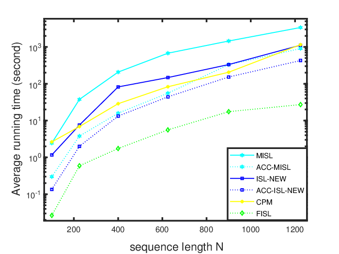
Figure. 6 consists of the comparison plots of average running time vs different sequence lengths for two different initializations. From simulation plots, one can observe that, irrespective of the sequence length and initialization, FISL algorithm is always taking less time when compared to the state-of-the-art algorithms. From figure-6(a), one can observe that the FISL algorithm is better than the MISL, ACC-MISL, ISL-NEW, ACC-ISL-NEW, and CPM algorithms by times respectively.
IV.Conclusion
In this paper, we address the problem, design of phase only sequences of arbitrary lengths by directly minimizing the ISL metric. We proposed a fast iterative algorithm by using the Majorization-Minimization method. Numerical simulations of the proposed algorithm were conducted for different sequence lengths using different initializations that confirm our algorithm performs better than the state-of-the-art algorithms in terms of the speed of convergence.
References
- [1] W. C. Knight, R. G. Pridham, and S. M. Kay, “Digital signal processing for sonar,” Proceedings of the IEEE, vol. 69, no. 11, pp. 1451–1506, Nov 1981.
- [2] M. Skolnik, “Radar handbook,” McGraw-Hill, 1990.
- [3] N. Levanon and E. Mozeson, “Basic radar signals,” John Wiley and Sons, vol. 64, no. 11, pp. 53–73, 2004.
- [4] P. Stoica, H. He, and J. Li, “Optimization of the receive filter and transmit sequence for active sensing,” IEEE Transactions on Signal Processing, vol. 60, no. 4, pp. 1730–1740, 2012.
- [5] J. Liang, L. Xu, J. Li, and P. Stoica, “On designing the transmission and reception of multistatic continuous active sonar systems,” IEEE Transactions on Aerospace and Electronic Systems, vol. 50, no. 1, pp. 285–299, 2014.
- [6] S. W. Golomb and G. Gong, Signal Design for Good Correlation: For Wireless Communication, Cryptography, and Radar. Cambridge University Press, 2005.
- [7] W. Roberts, H. He, J. Li, and P. Stoica, “Probing waveform synthesis and receiver filter design,” IEEE Signal Processing Magazine, vol. 27, no. 4, pp. 99–112, July 2010.
- [8] L. Zhao and D. P. Palomar, “Maximin joint optimization of transmitting code and receiving filter in radar and communications,” IEEE Transactions on Signal Processing, vol. 65, no. 4, pp. 850–863, 2017.
- [9] J. Khalife, K. Shamaei, and Z. M. Kassas, “Navigation with cellular cdma signals part i: Signal modeling and software-defined receiver design,” IEEE Transactions on Signal Processing, vol. 66, no. 8, pp. 2191–2203, 2018.
- [10] F. Gini, A. Maio, and L.Patton, Waveform Design and Diversity for Advanced Radar Systems. IET radar, sonar and navigation series, London, U.K.: Institution of Engineering and Technology, 2012.
- [11] S. Khalili, O. Simeone, and A. M. Haimovich, “Cloud radio-multistatic radar: Joint optimization of code vector and backhaul quantization,” IEEE Signal Processing Letters, vol. 22, no. 4, pp. 494–498, 2015.
- [12] W. Fan, J. Liang, G. Yu, H. C. So, and G. Lu, “Mimo radar waveform design for quasi-equiripple transmit beampattern synthesis via weighted -minimization,” IEEE Transactions on Signal Processing, vol. 67, no. 13, pp. 3397–3411, July 2019.
- [13] M. R. Bell, “Information theory and radar waveform design,” IEEE Transactions on Information Theory, vol. 39, no. 5, pp. 1578–1597, 1993.
- [14] T. D. Bhatt, E. G. Rajan, and P. V. D. S. Rao, “Design of high-resolution radar waveforms for multi-radar and dense target environments,” IET Radar, Sonar Navigation, vol. 5, no. 7, pp. 716–725, 2011.
- [15] Y. Li, S. Vorobyov, and Z. He, “Design of multiple unimodular waveforms with low auto- and cross-correlations for radar via majorization-minimization,” in Proceedings of the 24th European Signal Processing Conference, EUSIPCO 2016, ser. European Signal Processing Conference, vol. 2016-November. United States: IEEE, 11 2016, pp. 2235–2239.
- [16] O. Aldayel, V. Monga, and M. Rangaswamy, “Successive qcqp refinement for mimo radar waveform design under practical constraints,” IEEE Transactions on Signal Processing, vol. 64, no. 14, pp. 3760–3774, 2016.
- [17] X. Yu, K. Alhujaili, G. Cui, and V. Monga, “Mimo radar waveform design in the presence of multiple targets and practical constraints,” IEEE Transactions on Signal Processing, vol. 68, pp. 1974–1989, 2020.
- [18] J. J. Benedetto, I. Konstantinidis, and M. Rangaswamy, “Phase-coded waveforms and their design,” IEEE Signal Processing Magazine, vol. 26, no. 1, pp. 22–31, 2009.
- [19] P. Stoica, J. Li, and M. Xue, “Transmit codes and receive filters for radar,” IEEE Signal Processing Magazine, vol. 25, no. 6, pp. 94–109, 2008.
- [20] R. H. Barker, “Group synchronizing of binary digital systems,” Communication theory, pp. 273–287, 1953.
- [21] S. E. Kocabas and A. Atalar, “Binary sequences with low aperiodic autocorrelation for synchronization purposes,” IEEE Communications Letters, vol. 7, no. 1, pp. 36–38, Jan 2003.
- [22] R. Frank, “Polyphase codes with good nonperiodic correlation properties,” IEEE Transactions on Information Theory, vol. 9, no. 1, pp. 43–45, January 1963.
- [23] N. Zhang and S. W. Golomb, “Polyphase sequence with low autocorrelations,” IEEE Transactions on Information Theory, vol. 39, no. 3, pp. 1085–1089, May 1993.
- [24] P. Stoica, H. He, and J. Li, “On designing sequences with impulse-like periodic correlation,” IEEE Signal Processing Letters, vol. 16, no. 8, pp. 703–706, Aug 2009.
- [25] H. He, D. Vu, P. Stoica, and J. Li, “Construction of unimodular sequence sets for periodic correlations,” in 2009 Conference Record of the Forty-Third Asilomar Conference on Signals, Systems and Computers, Nov 2009, pp. 136–140.
- [26] A. Bose and M. Soltanalian, “Constructing binary sequences with good correlation properties: An efficient analytical-computational interplay,” IEEE Transactions on Signal Processing, vol. 66, no. 11, pp. 2998–3007, 2018.
- [27] M. Soltanalian and P. Stoica, “Computational design of sequences with good correlation properties,” IEEE Transactions on Signal Processing, vol. 60, no. 5, pp. 2180–2193, 2012.
- [28] P. Stoica, J. Li, and M. Xue, “On binary probing signals and instrumental variables receivers for radar,” IEEE Transactions on Information Theory, vol. 54, no. 8, pp. 3820–3825, 2008.
- [29] L. Tsai, W. Chung, and D. Shiu, “Synthesizing low autocorrelation and low papr ofdm sequences under spectral constraints through convex optimization and gs algorithm,” IEEE Transactions on Signal Processing, vol. 59, no. 5, pp. 2234–2243, 2011.
- [30] S. Mertens, “Exhaustive search for low-autocorrelation binary sequences,” Journal of Physics A: Mathematical and General, vol. 29, no. 18, pp. 473–481, sep 1996.
- [31] L. Zhao, J. Song, P. Babu, and D. P. Palomar, “A unified framework for low autocorrelation sequence design via majorization-minimization,” IEEE Transactions on Signal Processing, vol. 65, no. 2, pp. 438–453, Jan 2017.
- [32] L. K. Patton, S. W. Frost, and B. D. Rigling, “Efficient design of radar waveforms for optimised detection in coloured noise,” IET Radar, Sonar Navigation, vol. 6, no. 1, pp. 21–29, 2012.
- [33] P. Stoica, H. He, and J. Li, “New algorithms for designing unimodular sequences with good correlation properties,” IEEE Transactions on Signal Processing, vol. 57, no. 4, pp. 1415–1425, April 2009.
- [34] J. Song, P. Babu, and D. P. Palomar, “Optimization methods for designing sequences with low autocorrelation sidelobes,” IEEE Transactions on Signal Processing, vol. 63, no. 15, pp. 3998–4009, Aug 2015.
- [35] Y. Li and S. A. Vorobyov, “Fast algorithms for designing unimodular waveform(s) with good correlation properties,” IEEE Transactions on Signal Processing, vol. 66, no. 5, pp. 1197–1212, March 2018.
- [36] J. Song, P. Babu, and D. P. Palomar, “Sequence set design with good correlation properties via majorization-minimization,” IEEE Transactions on Signal Processing, vol. 64, no. 11, pp. 2866–2879, June 2016.
- [37] J. Liang, H. C. So, J. Li, and A. Farina, “Unimodular sequence design based on alternating direction method of multipliers,” IEEE Transactions on Signal Processing, vol. 64, no. 20, pp. 5367–5381, Oct 2016.
- [38] J. Song, P. Babu, and D. P. Palomar, “Sequence design to minimize the weighted integrated and peak sidelobe levels,” IEEE Transactions on Signal Processing, vol. 64, no. 8, pp. 2051–2064, April 2016.
- [39] M. A. Kerahroodi, A. Aubry, A. De Maio, M. M. Naghsh, and M. Modarres-Hashemi, “A coordinate-descent framework to design low psl/isl sequences,” IEEE Transactions on Signal Processing, vol. 65, no. 22, pp. 5942–5956, 2017.
- [40] R. Lin, M. Soltanalian, B. Tang, and J. Li, “Efficient design of binary sequences with low autocorrelation sidelobes,” IEEE Transactions on Signal Processing, vol. 67, no. 24, pp. 6397–6410, 2019.
- [41] L. Wu and D. P. Palomar, “Sequence design for spectral shaping via minimization of regularized spectral level ratio,” IEEE Transactions on Signal Processing, vol. 67, no. 18, pp. 4683–4695, 2019.
- [42] W. Fan, J. Liang, G. Yu, H. C. So, and G. Lu, “Minimum local peak sidelobe level waveform design with correlation and/or spectral constraints,” Signal Process., vol. 171, p. 107450, 2020.
- [43] W. Fan, J. Liang, H. C. So, and G. Lu, “Min-max metric for spectrally compatible waveform design via log-exponential smoothing,” IEEE Transactions on Signal Processing, vol. 68, pp. 1075–1090, 2020.
- [44] G. Cui, X. Yu, G. Foglia, Y. Huang, and J. Li, “Quadratic optimization with similarity constraint for unimodular sequence synthesis,” IEEE Transactions on Signal Processing, vol. 65, no. 18, pp. 4756–4769, 2017.
- [45] A. De Maio, S. De Nicola, Y. Huang, S. Zhang, and A. Farina, “Code design to optimize radar detection performance under accuracy and similarity constraints,” IEEE Transactions on Signal Processing, vol. 56, no. 11, pp. 5618–5629, 2008.
- [46] Z. Wang, P. Babu, and D. P. Palomar, “Design of par constrained sequences for mimo channel estimation via majorization minimization,” IEEE Transactions on Signal Processing, vol. 64, no. 23, pp. 6132–6144, 2016.
- [47] D. R. Hunter and K. Lange, “A tutorial on mm algorithms,” The American Statistician, vol. 58, no. 1, pp. 30–37, 2004. [Online]. Available: https://doi.org/10.1198/0003130042836
- [48] Y. Sun, P. Babu, and D. P. Palomar, “Majorization-minimization algorithms in signal processing, communications, and machine learning,” IEEE Transactions on Signal Processing, vol. 65, no. 3, pp. 794–816, Feb 2017.
- [49] H. Esmaeili-Najafabadi, M. Ataei, and M. F. Sabahi, “Designing sequence with minimum psl using chebyshev distance and its application for chaotic mimo radar waveform design,” IEEE Transactions on Signal Processing, vol. 65, no. 3, pp. 690–704, 2017.
- [50] M. M. Naghsh, M. Soltanalian, P. Stoica, M. Modarres-Hashemi, A. De Maio, and A. Aubry, “A doppler robust design of transmit sequence and receive filter in the presence of signal-dependent interference,” IEEE Transactions on Signal Processing, vol. 62, no. 4, pp. 772–785, 2014.
- [51] G. Cui, Y. Fu, X. Yu, and J. Li, “Local ambiguity function shaping via unimodular sequence design,” IEEE Signal Processing Letters, vol. 24, no. 7, pp. 977–981, 2017.
- [52] Y. Jing, J. Liang, B. Tang, and J. Li, “Designing unimodular sequence with low peak of sidelobe level of local ambiguity function,” IEEE Transactions on Aerospace and Electronic Systems, vol. 55, no. 3, pp. 1393–1406, June 2019.
- [53] A. Aubry, A. De Maio, B. Jiang, and S. Zhang, “Ambiguity function shaping for cognitive radar via complex quartic optimization,” IEEE Transactions on Signal Processing, vol. 61, no. 22, pp. 5603–5619, 2013.
- [54] L. Wu, P. Babu, and D. P. Palomar, “Cognitive radar-based sequence design via sinr maximization,” IEEE Transactions on Signal Processing, vol. 65, no. 3, pp. 779–793, 2017.
- [55] W. Fan, J. Liang, and J. Li, “Constant modulus mimo radar waveform design with minimum peak sidelobe transmit beampattern,” IEEE Transactions on Signal Processing, vol. 66, no. 16, pp. 4207–4222, 2018.
- [56] H. Wolkowicz and G. P. Styan, “Bounds for eigenvalues using traces,” Linear Algebra and its Applications, vol. 29, pp. 471–506, 1980, special Volume Dedicated to Alson S. Householder. [Online]. Available: http://www.sciencedirect.com/science/article/pii/002437958090258X
- [57] D. Bertsekas, A. Nedić, and A. Ozdaglar, Convex Analysis and Optimization, ser. Athena Scientific optimization and computation series. Athena Scientific, 2003. [Online]. Available: https://books.google.co.in/books?id=DaOFQgAACAAJ