Observable features in (ultra)high energy neutrinos due to active-sterile secret interactions

It is well known that mesons can decay leptonically as $M\to\nu_{\ell}\ell$, where $M$ represents a meson ($\pi^{+},\,K^{+},\,D^{+}$) and $\ell=e,\mu,\tau$ depending on the meson. The interaction given in eq. (1) opens the possibility of new leptonic decay channels: $M\to\nu_{s}\ell\varphi$ and $M\to\nu_{s}\ell\overline{\nu}_{\ell^{\prime}}\nu_{s}$. The Feynman diagrams for these new decay channels are shown in Figure 1. In this regard, we would like to remark that our assumption of small active-sterile mixing angle is crucial, since it prevents the appearance of new decay channels such as $M\to\nu_{\ell^{\prime}}\ell\varphi$.

Concerning the process $M\to\nu_{s}\ell\varphi$, it becomes possible only if the corresponding $\lambda_{\ell}\neq 0$; moreover, it is kinematically allowed only if

where $m_{M}$ is the mass of the decaying meson and $m_{\ell}$ the mass of charged lepton $\ell$. A lower limit on $m_{s}+M_{\varphi}$ arises from Big Bang Nucleosynthesis as discussed below. Using the relation (4), in table (1) we provide the maximal allowed values for $m_{s}+M_{\varphi}$, namely $m_{M}-m_{\ell}$.

We observe that $\pi^{+},K^{+},D^{+}\to e\varphi\nu_{s}$ and $K^{+},D^{+}\to\mu\varphi\nu_{s}$ have a large phase space available, while $\pi^{+}\to\mu\varphi\nu_{s}$ and $D^{+}\to\tau\varphi\nu_{s}$ are only marginally allowed. At last, the processes $\pi^{+},K^{+}\to\tau\varphi\nu_{s}$ are not kinematically allowed.
In the active sector, experimental bounds on meson decay provide limits on $\lambda_{\ell}$, see for example Berryman et al. 2018, where similar processes involving active neutrinos $\nu_{\ell}$ have been studied in details. The main difference between our case and the one studied in Berryman et al. 2018 is that the relation (4) is replaced with $M_{\varphi}\lesssim m_{M}-m_{\ell}$. In Berryman et al. 2018, the limit on $\lambda_{\mu}$ from $K^{+}\to\mu\varphi\nu_{s}$ has been found to be stronger with respect to the limit on $\lambda_{e}$ from $K^{+}\to e\varphi\nu_{s}$. This depends on the more accurate experimental data available for the former process compared to the latter. Moreover, for masses of the scalar field $\varphi$ smaller than about $300$ MeV, the limits on $\lambda_{e,\mu}$ from $K^{+}$ decay are stronger compared to the one from $\pi^{+}$ and $D^{+}$ mesons decay. Concerning the $\lambda_{\tau}$ coupling, $\pi^{+}$ and $K^{+}$ can not provide information because of kinematics, see table (1). We have explicitly analyzed the rate of process $D^{+}\to\tau\varphi\nu_{s}$, finding that it is very small compared with the experimental bounds. Therefore, we find that for masses $M_{\varphi}$ and $m_{s}$ consistent with the cosmological constraints, $\lambda_{\tau}=1$ is always allowed.

In addition to three-body decay $M\to\nu_{s}\ell\varphi$ discussed above, there is a further decay channel which occurs as a result of the new interaction: the four-body decay, $M\to\nu_{s}\ell\overline{\nu}_{\ell^{\prime}}\nu_{s}$. In this case the kinematics only constrains the mass of the sterile neutrino. In particular, the decay is kinematically allowed if

If $\lambda<1,$the rate for four-body decay will be smaller by a factor of $\lambda^{2}$ compared to the three-body decay²² 2 By $\lambda$ we mean the larger of the three couplings $\lambda_{\alpha}$.. We therefore expect that the four-body decay can relevantly change the exclusions in the parameter space only if $\lambda=1$. Later we will explicitly verify the validity of the assertion.

We now discuss the explicit form of the decay rate of mesons through the new interactions. As a benchmark case we will discuss the Kaon decay into the muon channel: however, it is straightforward to obtain the decay rate for a different meson decay $M$ into the leptonic channel $\alpha$ by simply replacing in all the subsequent formulas $M_{K}$ by $m_{M}$ and $\mu$ by $\alpha$.

We begin by examining the three body decay $K^{+}\to\mu\nu_{s}\varphi$. In the limit of vanishing active neutrino masses, the decay rate is

where

We have defined with $p$, $q$, $k$ and $P$ respectively the $\mu$, $\varphi$, $\nu_{s}$ and $K$ four-momenta, and in bold face their spatial three-momenta. $f_{K}$ is the Kaon decay form factor.

With an analogous notations for the four body decay $K^{+}\to\mu\nu_{s}\nu_{s}\overline{\nu}_{\ell}^{\prime}$, the decay rate can then be written:

where $p$, $q$, $l$, $k$ and $P$ denote the four-momenta respectively of $\mu$, $\nu_{s}$, $\nu_{\ell}^{\prime}$, $\nu_{s}$ and $K$. For convenience, we also defined $s=P-p$. We have also defined

In this case, there are $5$ independent variables to parameterize the decay, which we choosed to be $|\mathbf{p}|$, $|\mathbf{q}|$, $|\mathbf{k}|$, the angle $\theta$ between $\mathbf{p}$ and $\mathbf{q}$, and the azimuthal angle $\phi$ between $\mathbf{k}$ and the plane determined by $\mathbf{p}$ and $\mathbf{q}$. In case $\mathbf{p}$ and $\mathbf{q}$ were collinear, this should be interpreted as the azimuthal angle around the direction of $\mathbf{p}$

Both the processes $K^{+}\to\mu\varphi\nu_{s}$ and $K^{+}\to\mu\nu_{s}\nu_{s}\overline{\nu}_{\ell}^{\prime}$ should be observed as $K\to\mu+\mbox{missing energy}$. The closer Kaon decay process that is reported into PDG et al. 2018 is $K\to\mu\nu\overline{\nu}\nu$ that can be used to constrain our processes. Therefore, we impose that the branching ratio to this channels should be smaller than $2.4\times 10^{-6}$ et al. 2018.

As mentioned in section II, a reasonable choice for a qualitative picture of the general case is to take $\lambda_{e}=\lambda_{\mu}=\lambda_{\tau}=\lambda$. In Figure 2 we consider this case and we show the region excluded by Kaon decay in the $M_{\varphi}-m_{s}$ plane for various values of the coupling.

From figure (2) we observe that if

then the correction to Kaon decay is within the experimental bound.

The four-body decay channel only produces a bump in the right part of the exclusion contours, corresponding to a roughly horizontal line of exclusion that only constrains $m_{s}$, as expected from our previous considerations: just as we had deduced, this bump is only relevant for $\lambda=1$.

The only case in which the results are drastically different from the choice of equal couplings for the three flavors is the one in which $\lambda_{\tau}\neq 0$ and the other two couplings are much smaller than it. In fact, as we mentioned above, this case is unconstrained from meson physics and even for value of $\lambda_{\tau}\sim\mathcal{O}(1)$ the only relevant bound in the $M_{\varphi}-m_{s}$ plane comes from Big Bang Nucleosynthesis as discussed below.

In addition to laboratory bounds, there could be additional constraints coming from cosmology at different epochs of the Universe. A first constraint comes from the Big Bang Nucleosynthesis (BBN) epoch and specifically from the number of relativistic degrees of freedom. In particular, the requirement is that there are no extra relativistic species (apart from the ones predicted from the Standard Model) at the moment of the BBN. This naturally happens if the new introduced species $\varphi$ and $\nu_{s}$ are non relativistic and in thermal equilibrium before and during BBN. Indeed, their distributions will be then Boltzmann suppressed by a factor of $e^{-m/T_{\rm BBN}}$, where $T_{\rm BBN}\simeq 1$ MeV, and will not count as extra degree of freedom. Another constraint comes from the requirement that the new interaction does not affect the free-streaming nature (non interacting) of the active neutrinos at the time of the formation of the Cosmic Microwave Background (CMB).

A full discussion of the cosmological bounds would require explicit solution of the evolution equations for all the relevant species and is outside the scope of this work. We will limit ourselves to an order of magnitude estimate of the rates of the relevant processes to get a clear idea of which portion of the parameter space is effectively constrained. Therefore, we did not distinguish between the three different coupling $\lambda_{\alpha}$ but we used an effective coupling $\lambda$. This latter have been chosen as the largest coupling between the three and so the most relevant.

As mentioned above, the requirements to not affect the BBN yields are that the newly introduced species are non relativistic at the time of the BBN and that they remain in kinetic and chemical equilibrium throughout the passage from relativistic to non relativistic. The first requirement is naturally met if both $M_{\varphi}$ and $m_{s}$ are chosen to be larger than about $10$ MeV: in this way, the Boltzmann factor is smaller than $10^{-4}$ and we can safely assume that the species are non relativistic. Concerning the second requirement, is necessary to compare the rates of the processes responsible for the equilibrium with the rate of the expansion of the Universe, in order to determine the temperature of decoupling at which such processes become irrelevant.

• •

  $\nu_{\alpha}\nu_{s}\to\nu_{\alpha}\nu_{s}$ and $\nu_{s}\nu_{s}\to\nu_{\alpha}\nu_{\alpha}$: the cross section of these processes, mediated by $\varphi$, can be estimated as $\frac{\lambda^{4}T^{2}}{M_{\varphi}^{4}}$ . If we assume a non relativistic distribution for the particles involved, consistently with our requirement that the newly introduced species decouples while being non relativistic, the sterile number density grows as $n\sim(Tm_{s})^{3/2}e^{-m_{s}/T}$. The decoupling temperature will be set by the condition $n\sigma\sim H$, where $H$ is the Hubble parameter, which translates into the condition $n\sigma\sim\frac{T^{2}}{M_{Pl}}$, where $M_{Pl}$ is the Planck mass. This leads to the relation

  $$\left(\frac{T}{m_{s}}\right)^{3/2}e^{-m_{s}/T}\sim\frac{M_{\varphi}^{4}}{M_{Pl}m_{s}^{3}\lambda^{4}}.$$

  An approximate solution for this equation, in the regime in which $M_{Pl}m_{s}^{3}\lambda^{4}\gg M_{\varphi}^{4}$, is then

  $$T_{s}\sim\frac{m_{s}}{\log\left[\frac{M_{Pl}m_{s}^{3}\lambda^{4}}{M_{\varphi}^{4}}\right]}.$$

  The factor in the denominator depends only logarithmically, and therefore very weakly, on the parameters, and for typical values of the masses between $10$ MeV and $1$ GeV and $\lambda$ between $0.01$ and $1$ is of the order of $10$ to $100$. Therefore we find that the decoupling temperature is of the order of $\frac{m_{s}}{10}$, which means that these processes are able to maintain both kinetic and chemical equilibrium between active and sterile neutrinos even after the latter have become non relativistic, ensuring the Boltzmann suppression of this species.

• •

  $\varphi\varphi\to\nu_{s}\nu_{s}$ or $\varphi\varphi\to\nu_{\alpha}\nu_{\alpha}$: the most efficient is the first process mediated by active neutrino. The cross section is estimated as $\frac{\lambda^{4}}{m_{\alpha}^{2}}$, where $m_{\alpha}$ is the active neutrino mass, and if we again assume a non relativistic distribution for the scalar particles we find the condition

  $$\left(\frac{T}{M_{\varphi}}\right)^{-1/2}e^{-M_{\varphi}/T}\sim\frac{m_{\alpha}^{2}}{M_{Pl}M_{\varphi}\lambda^{4}}.$$

  An approximate expression for the decoupling temperature, in the regime $m_{\alpha}^{2}\ll M_{\varphi}M_{Pl}\lambda^{4}$, is

  $$T_{\varphi}\sim\frac{M_{\varphi}}{\log\left[\frac{M_{\varphi}M_{Pl}\lambda^{4}}{m_{\alpha}^{2}}\right]}.$$

  Since the factor in the denominator is typically of order $10$ to $100$, we find again that the scalar particles remain in equilibrium throughout their passage from relativistic to non relativistic, and they therefore become Boltzmann suppressed, not counting as radiative degrees of freedom.

In summary, for the parameter space which is of interest to us, both scalar and sterile particles remain in kinetic and chemical equilibrium throughout the primordial nucleosynthesis. By taking them sufficiently massive, namely

we can safely satisfy BBN limits, since the newly introduced particles are so massive that they are Boltzmann suppressed during BBN.

At the time of formation of the Cosmic Microwave Background (CMB), sterile neutrinos and scalar particles have long disappeared. Active neutrinos, though, can still secretly interact through the reactions $\nu_{\alpha}\nu_{\alpha^{\prime}}\to\nu_{\beta}\nu_{\beta^{\prime}}$. There are in principle two ways in which this interaction can proceed through the new interaction: either the mixing angle between active and sterile neutrinos is sufficiently large, so that the process $\nu_{\alpha}\nu_{s}\to\nu_{\alpha}\nu_{s}$ can be converted via mixing to a four active neutrino process; or the process can happen at next-to-leading order via the box diagram. We will only analyze the latter process, since we have assumed very small mixing angles between active and sterile neutrinos. We assume a relativistic distribution for the active neutrinos. The cross section can be estimated in order of magnitude as $\frac{\lambda^{8}T^{10}}{M_{\varphi}^{8}m_{s}^{4}}$, so that the decoupling temperature for this process is

In order to guarantee free-streaming active neutrinos at CMB time, $T^{\rm dec}$ has to be larger than the temperature of CMB formation, around $1$ eV. We have checked that this is the case for all the parameter space we considered.

Another possible constraint we should take into account comes from the analysis of neutrino fluxes from supernovae. This kind of constraints have been recently taken into account in the analysis of active-active secret interactions Mastrototaro et al. 2020; Shalgar et al. 2019. In fact, since neutrinos in the supernovae core have energies of order of tens or hundreds of MeV, they are sufficiently energetic to produce non relativistic sterile neutrinos. If these sterile neutrinos interact sufficiently weakly with the active neutrinos in the core, they could escape the supernova giving rise to an observable energy loss. The conditions for this to happen are two: in the first place, the mean free path of the sterile neutrino inside the core, namely $\left(\sigma_{sa}n_{a}\right)^{-1}$, with $\sigma_{sa}$ the cross section and $n_{a}$ the number density of active neutrinos in the core, should be larger than the radius of the supernova core, typically around $10$ km. The cross section is evaluated for active neutrinos with typical energies of tenth of MeV and sterile neutrinos at rest. The number density $n_{a}$ can be estimated assuming a thermal distribution $f(E)$ of active neutrinos, with a typical temperature of tenth of MeV, as in Mastrototaro et al. 2020.

The second condition to be verified is that sterile neutrinos should be copiously produced in the supernova core and that the energy injected into sterile neutrinos can exceed the threshold luminosity $L_{s}\simeq 2\times 10^{52}$ erg/s (namely $L_{s}\simeq 8.2\times 10^{36}$ MeV² in natural units, which we have used throughout this work) for the supernova SN 1987A Mastrototaro et al. 2020. We then estimate the luminosity in the proposed model as:

where $f(E,r)$ is the distribution of active neutrinos inside the core of the supernova. The temperature profile $T(r)$ is taken from Mastrototaro et al. 2020.

The model under consideration could be in conflict with SN 1987A data if both the above conditions would simultaneously met. We have numerically verified that this situation never occurs for all the parameter space we considered, with $m_{s}$ and $M$ larger than $10$ MeV. Indeed, for large values of the coupling $\lambda$ the energy injected into sterile sector can easily exceed the threshold indicated above, but the interaction between sterile and active neutrinos is so strong that the mean free path is much shorter than the supernova dimensions. For small values of $\lambda$ we encounter the opposite situation where, even if sterile neutrinos are practically free to escape the supernova, they are produced in too small amounts to be observable. We can therefore deduce that the model we consider is not constrained by supernova data.

We consider a collection of astrophysical neutrino sources, each one producing a power law spectrum per unit solid angle⁴⁴ 4 If the source is anisotropic, the spectrum is evaluated in the direction of the Earth. in energy

where $g\equiv\phi_{\nu_{e}}+\phi_{\nu_{\mu}}+\phi_{\nu_{\tau}}+\phi_{\overline{\nu}_{e}}+\phi_{\overline{\nu}_{\mu}}+\phi_{\overline{\nu}_{\tau}}$ and $\gamma$ is the spectral index. The IceCube analysis gives as best fit value for the throughgoing muons data set $\gamma=2.28$ Schneider 2020. Due the similarity with the cosmogenic neutrino production, we found convenient to adopt the Star Forming rate $\rho(z)$ Hopkins and Beacom 2006 for the cosmological evolution of these sources, where $\rho(z)$ is defined as the comoving number density. The normalization $\mathcal{N}$ is chosen in such a way as to reproduce the best fit for the diffuse neutrino flux measured by the IceCube Collaboration in the throughgoing muons data sample. The flux arriving at Earth from the point-like source, expressed in terms of $g(E)$, is

where $r(z)=\int_{0}^{z}\frac{dz^{\prime}}{H(z^{\prime})}$.
Therefore, the diffuse astrophysical spectrum is written as

We assume for definiteness a flavor structure at the source $(1:2:0)$, corresponding to pion beam sources.

Throughout our analysis we use the best fit values from the NuFit 3.2 global fit data for the active oscillation parameters Esteban et al. 2017, assuming normal neutrino mass ordering.

Cosmogenic neutrinos are produced by the scattering of high energy protons from the cosmic rays with the CMB photons. The production of cosmogenic neutrinos is quantitatively studied, for example, in Ahlers and Halzen 2012. In our previous work Fiorillo et al. 2020 we showed that their results can be reproduced by parameterizing the cosmogenic neutrino spectrum as

where $\rho(z)$ is the Star Forming rate Hopkins and Beacom 2006. We refer the reader to Fiorillo et al. 2020 for the method of determination of the function $f(E)$ describing the energy spectrum.

For cosmogenic neutrinos we again assume a flavor structure at the source $(1:2:0)$.

Because of the secret interactions, active neutrinos can collide with active neutrinos from the CNB, producing sterile neutrinos and thereby causing a depletion of the flux observable at Earth. The transport equation for active neutrinos is in principle coupled to the transport equation for sterile neutrinos, since the secret interactions produce sterile neutrinos which can in turn collide with other CNB neutrinos to regenerate part of the original flux. The form of these equations has been given in Fiorillo et al. 2020, and we reproduce it here for the generalized multiflavor case. We define with $\Phi_{i}(z,E)$ the flux of active neutrinos in the $i$th ($i=1,2,3$) mass eigenstate per unit energy interval per unit solid angle at a redshift $z$, while $\Phi_{s}(z,E)$ denotes the flux of sterile neutrinos, where in absence of mixing the sterile mass eigenstate is indicated with $s$. The flux at Earth is connected with the flux at generic redshift by the relation $\frac{d\phi_{\nu}}{dEd\Omega}=\Phi(0,E)$. We write separate equations for the mass eigenstates because, as discussed in Fiorillo et al. 2020, the propagation is diagonal in the mass eigenstates, given the path between collisions much larger than the oscillation lengths. In other words, due to the very fast oscillations caused by mixing, in between two collisions, a neutrino decoheres to mass eigenstates.

The transport equations take the form:

where $f(E)$ is the neutrino spectrum produced at the source and $\xi_{i}$ is the fraction of neutrinos produced at the source in the $i$th mass eigenstate. Similarly, for the sterile flux we write:

For convenience, we have denoted by $\sigma_{i}$ and $\sigma_{s}$ the cross sections for the collision of an $i$th mass eigenstate and a sterile neutrino, respectively, with a CNB neutrino. Correspondingly, $\frac{d\sigma_{\alpha\beta}}{dE}(E^{\prime}\to E)$ is the cross section for the production of a $\beta$ neutrino with energy $E$ after the collision of a $\alpha$ neutrino with energy $E^{\prime}$ with a CNB neutrino. However, it is important to notice that if $m_{s}>M_{\varphi}$, a further process needs to be taken into account corresponding to the possible decay of the sterile neutrinos into an active neutrino and a scalar mediator. We refer the reader to Appendix B for the mathematical treatment of this case.

If the regeneration processes play an important role, the task of determining the effect of the interaction is computationally expensive, since it requires the numerical solution of the system of four coupled partial integro-differential equations

In our previous paper Fiorillo et al. 2020, we found that the regeneration was unimportant for a limited region of the parameter space, with masses of sterile neutrino and scalar mediator around $250$ MeV. Here we have analyzed this question more thoroughly, taking in consideration a wider parameter space. We have adopted a perturbative approach in which the regeneration processes are treated as a perturbation and we have tested its validity a posteriori by comparing the perturbation induced by regeneration with the unperturbed flux.

We find that both cosmogenic and astrophysical fluxes are practically unaffected by regeneration. The physical reason behind this behavior is connected with the cosmological evolution of the sources, and in particular with the fact that the sources are distributed at various redshifts. In fact, while neutrinos produced at high redshifts, with $z\gg 0.1$, are severely suppressed due to the absorption on the CNB, neutrinos produced at low redshifts are only weakly absorbed. Thus the flux has always a component, produced at low redshift, which is roughly unabsorbed and which dominates against the small regenerated flux produced at high redshifts. The perturbative approach shows in fact that the corrections coming from regeneration, both for cosmogenic and astrophysical fluxes, are typically not larger than about $10\%$. This conclusion is not reached in the case $m_{s}>M_{\varphi}$, where sterile neutrino decays are important, as described in Appendix B. In this case, we find that the results of the first order perturbation theory may cause small but non negligible changes to the spectrum. For this reason, in the following the regime $m_{s}>M_{\varphi}$ has been treated taking into account regeneration perturbatively to first order.

The negligible effect of regeneration is therefore connected with the presence of sources at small redshifts, masquerading the regenerated flux. Thus we expect that, for point-like sources localized at large redshifts, regeneration effects should instead be non negligible. Even though IceCube has identified so far a single realistic candidate of point-like astrophysical source, in the future one may expect noticeable improvements in this respect. Therefore, it might be interesting to have a qualitative idea of the effect of regeneration on the neutrino spectra from point-like sources. In Figure 3 we show the spectra expected at Earth for a generic source at two fixed redshift values $z$, namely $0.1$ and $0.01$, with an $E^{-2}$ reference spectrum. The effects of regeneration are, as expected, more important for larger redshifts of the source and can drastically change the results.

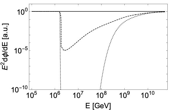
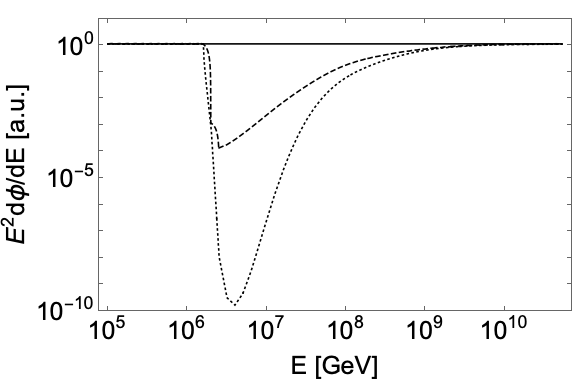
In the following, since we only deal with cosmogenic and astrophysical neutrino fluxes, we neglect the regeneration processes, so that the transport equation for the sole active neutrinos is given by

In this equation $\sigma_{i}$ is the cross section of the process $\nu_{i}+\nu_{j}\to\nu_{s}+\nu_{s}$, namely

in terms of the Mandelstam invariants $s=(p+l)^{2}$, $t=(p-k)^{2}$ and $u=(p-q)^{2}$ with $p$, $l$, $k$ and $q$ the momentum of the two active neutrinos and the two sterile neutrinos, respectively. Moreover

and

where $m$ is the mass of the active neutrino $\nu$ of CNB. The squared amplitude is given by

where $\Gamma$ is the decay rate of the scalar mediator and $M_{\varphi}$ is its mass.

Therefore eq.(18) contains only an absorption term and, for the astrophysical power law neutrino flux, it admits an analytical solution for the flux at Earth given by

For cosmogenic neutrino fluxes the solution is identical with we consider the function $f(E)$ in place of $g(E)$.

We start our discussion of the results with the case of a power law astrophysical spectrum in the energy range roughly below $100$ PeV. In this region the effects of active-sterile interaction can be detected only if the sterile mass is sufficiently low that the process is not kinematically forbidden. As in the previous sections, we distinguish between the two possibilities: either $\lambda_{e}=\lambda_{\mu}=\lambda_{\tau}=\lambda_{af}$ (where $af$ denotes all flavors), or $\lambda_{e}=\lambda_{\mu}=0$ and $\lambda_{\tau}\neq 0$.

In the first case, the Kaon decay strongly constrains the possible values of the coupling. In particular, we find that the optimal choice to have noticeable effects below $100$ PeV is to have small sterile masses, large scalar masses and $\lambda_{af}=1$. We take as benchmark values $m_{s}=10$ MeV and $M_{\varphi}=1$ GeV.

In the second case, in which the mediator only couples to tau neutrinos, the constraints from meson decays are irrelevant and we can also consider lower masses for $M_{\varphi}$. In order to maximize the effect in this energy range, we have chosen the benchmark values of $m_{s}=15$ MeV, $M_{\varphi}=10$ MeV and $\lambda_{\tau}=1$, as represented in Fig, 4 where we show the neutrino spectra after the new interaction for both the choices of $\lambda$, together with the IceCube HESE data Peretti et al. 2020. From this Figure we can infer that the second possibility is already testable using IceCube data while the first case is essentially undistinguishable from the power-law in the energy range probed by IceCube.

An interesting aspect revealed by Figure 4 is that the new interaction causes a cutoff-like feature in the spectrum in the range between $1$ PeV and $10$ PeV. In fact, the second case with only $\lambda_{\tau}$, shows a sudden drop of the flux at the energy at which the process $\nu_{\alpha}\nu_{\beta}\to\nu_{s}\nu_{s}$ becomes kinematically allowed.

We also emphasize that, in the case $m_{s}=15$ MeV, $M_{\varphi}=10$ MeV, where regeneration may slightly change the results because of the presence of sterile neutrino decays, in addition to the absorption, there is a small pile up of neutrinos in the region between $100$ TeV and $1$ PeV. As mentioned before, this result has been obtained using first order perturbation theory for the treatment of the regeneration term.

The effects of the new interaction can also cause significant changes in the flavor structure of the spectrum since the induced depletion acts differently on each flavor modifying the flavor ratio, namely the fraction of electron, muon and tau neutrino fluxes. Since the depletion is energy dependent, the result will be an energy dependent flavor ratio. In Figures 5 we show the flavor ratios as a function of the energy for the two cases, $\lambda_{af}$ and $\lambda_{\tau}$ respectively. We see that the case of only $\lambda_{\tau}$ has a threshold behavior with a sudden change of the flavor ratio. This change is quite relevant, especially when compared with the change in the case $\lambda_{af}$. We remind the reader that we assumed a flavor ratio at the source $(1:2:0)$: at low energies, where the effects of the interaction are inactive, we recover the typical flavor structure $(1:1:1)$ at the Earth as expected.

The effects of secret interaction on the flavor structure of the spectrum, namely the modifications of the flavor ratio, can also be represented in the flavor triangle: we show this for case $\lambda_{\tau}=1$, which has the largest effect, in Figure 6.
The red and the orange points correspond to an energy of $10^{5}$ GeV and $10^{8}$ GeV, respectively. The flavor sensitivity which has been forecasted for IceCube-Gen2 Bustamante and Ahlers 2019, in the case of pion beam sources with a flavor ratio $(1:2:0)$ at the source, has been shown as well. The triangle representation suggests the possibility that future experiments might be able to unveil a different flavor structure possibly caused by active-sterile secret interactions. It is worth noticing that this change induced by the interaction is also dominant with respect to the uncertainty due to the mixing parameters.
A fundamental feature of the change in flavor induced by secret interactions is that it has a unique energy dependence, which descends from the resonances and thresholds of the interaction. Since the data from IceCube-Gen2 might allow in the future to investigate the interplay between flavor and energy, this is a result which might be of experimental interest.

For the case of cosmogenic fluxes, which are relevant at higher energies, the absorption effect is most important for higher masses of the sterile neutrino and of the scalar mediator. In this part of the parameter space, the constraints from mesons decay are substantially irrelevant, so there is no need to distinguish between the two case studied above. We will therefore analyze as a single choice the case $\lambda_{e}=\lambda_{\mu}=\lambda_{\tau}=1$, $m_{s}=250$ MeV and $M_{\varphi}=250$ MeV. In Figure 7 we show the effect of the interaction on the cosmogenic flux. We can observe that the effect is maximal around $10^{9\div 10}$ GeV. We address the reader to our previous paper Fiorillo et al. 2020 for more details also in relation to future experiments.

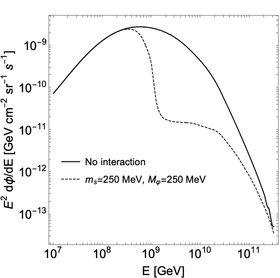
As in the astrophysical neutrino case, also for the cosmogenic flux we analyze the flavor structure as a function of energy, as shown in Figures 8.

References

- Winter (2013) W. Winter, Phys. Rev. D 88, 083007 (2013), arXiv:1307.2793 [astro-ph.HE] .
- Murase et al. (2016) K. Murase, D. Guetta, and M. Ahlers, Phys. Rev. Lett. 116, 071101 (2016), arXiv:1509.00805 [astro-ph.HE] .
- Loeb and Waxman (2006) A. Loeb and E. Waxman, JCAP 05, 003 (2006), arXiv:astro-ph/0601695 .
- Murase et al. (2013) K. Murase, M. Ahlers, and B. C. Lacki, Phys. Rev. D 88, 121301 (2013), arXiv:1306.3417 [astro-ph.HE] .
- Tamborra et al. (2014) I. Tamborra, S. Ando, and K. Murase, JCAP 09, 043 (2014), arXiv:1404.1189 [astro-ph.HE] .
- Bechtol et al. (2017) K. Bechtol, M. Ahlers, M. Di Mauro, M. Ajello, and J. Vandenbroucke, Astrophys. J. 836, 47 (2017), arXiv:1511.00688 [astro-ph.HE] .
- Berezinsky and Zatsepin (1969) V. S. Berezinsky and G. T. Zatsepin, Phys. Lett. 28B, 423 (1969).
- Berezinsky et al. (1998) V. Berezinsky, P. Blasi, and A. Vilenkin, Phys. Rev. D58, 103515 (1998), arXiv:astro-ph/9803271 [astro-ph] .
- Nagano and Watson (2000) M. Nagano and A. A. Watson, Rev. Mod. Phys. 72, 689 (2000).
- Engel et al. (2001) R. Engel, D. Seckel, and T. Stanev, Phys. Rev. D64, 093010 (2001), arXiv:astro-ph/0101216 [astro-ph] .
- Kusenko and Weiler (2002) A. Kusenko and T. J. Weiler, Phys. Rev. Lett. 88, 161101 (2002), arXiv:hep-ph/0106071 [hep-ph] .
- Anchordoqui et al. (2003) L. Anchordoqui, T. C. Paul, S. Reucroft, and J. Swain, Int. J. Mod. Phys. A18, 2229 (2003), arXiv:hep-ph/0206072 [hep-ph] .
- Fodor et al. (2002) Z. Fodor, S. D. Katz, and A. Ringwald, JHEP 06, 046 (2002), arXiv:hep-ph/0203198 [hep-ph] .
- Kalashev et al. (2002) O. E. Kalashev, V. A. Kuzmin, D. V. Semikoz, and G. Sigl, Phys. Rev. D66, 063004 (2002), arXiv:hep-ph/0205050 [hep-ph] .
- Semikoz and Sigl (2004) D. V. Semikoz and G. Sigl, JCAP 0404, 003 (2004), arXiv:hep-ph/0309328 [hep-ph] .
- Fodor et al. (2003) Z. Fodor, S. D. Katz, A. Ringwald, and H. Tu, JCAP 0311, 015 (2003), arXiv:hep-ph/0309171 [hep-ph] .
- Ave et al. (2005) M. Ave, N. Busca, A. V. Olinto, A. A. Watson, and T. Yamamoto, Astropart. Phys. 23, 19 (2005), arXiv:astro-ph/0409316 [astro-ph] .
- Seckel and Stanev (2005) D. Seckel and T. Stanev, Phys. Rev. Lett. 95, 141101 (2005), arXiv:astro-ph/0502244 [astro-ph] .
- De Marco et al. (2006) D. De Marco, T. Stanev, and F. W. Stecker, Phys. Rev. D73, 043003 (2006), arXiv:astro-ph/0512479 [astro-ph] .
- Allard et al. (2006) D. Allard, M. Ave, N. Busca, M. A. Malkan, A. V. Olinto, E. Parizot, F. W. Stecker, and T. Yamamoto, JCAP 0609, 005 (2006), arXiv:astro-ph/0605327 [astro-ph] .
- Becker (2008) J. K. Becker, Phys. Rept. 458, 173 (2008), arXiv:0710.1557 [astro-ph] .
- Anchordoqui et al. (2007) L. A. Anchordoqui, H. Goldberg, D. Hooper, S. Sarkar, and A. M. Taylor, Phys. Rev. D76, 123008 (2007), arXiv:0709.0734 [astro-ph] .
- Berezinsky et al. (2011) V. Berezinsky, A. Gazizov, M. Kachelriess, and S. Ostapchenko, Phys. Lett. B695, 13 (2011), arXiv:1003.1496 [astro-ph.HE] .
- Ahlers et al. (2010) M. Ahlers, L. A. Anchordoqui, M. C. Gonzalez-Garcia, F. Halzen, and S. Sarkar, Astropart. Phys. 34, 106 (2010), arXiv:1005.2620 [astro-ph.HE] .
- Katz and Spiering (2012) U. F. Katz and C. Spiering, Prog. Part. Nucl. Phys. 67, 651 (2012), arXiv:1111.0507 [astro-ph.HE] .
- Gelmini et al. (2012) G. B. Gelmini, O. Kalashev, and D. V. Semikoz, JCAP 1201, 044 (2012), arXiv:1107.1672 [astro-ph.CO] .
- Ng and Beacom (2014) K. C. Y. Ng and J. F. Beacom, Phys. Rev. D90, 065035 (2014), [Erratum: Phys. Rev.D90,no.8,089904(2014)], arXiv:1404.2288 [astro-ph.HE] .
- Murase (2015) K. Murase, Proceedings, 26th International Conference on Neutrino Physics and Astrophysics (Neutrino 2014): Boston, Massachusetts, United States, June 2-7, 2014, AIP Conf. Proc. 1666, 040006 (2015), arXiv:1410.3680 [hep-ph] .
- Heinze et al. (2016) J. Heinze, D. Boncioli, M. Bustamante, and W. Winter, Astrophys. J. 825, 122 (2016), arXiv:1512.05988 [astro-ph.HE] .
- Aloisio et al. (2015) R. Aloisio, D. Boncioli, A. di Matteo, A. F. Grillo, S. Petrera, and F. Salamida, JCAP 1510, 006 (2015), arXiv:1505.04020 [astro-ph.HE] .
- Halzen (2016) F. Halzen, Nature Phys. 13, 232 (2016).
- Cherry and Shoemaker (2019) J. F. Cherry and I. M. Shoemaker, Phys. Rev. D99, 063016 (2019), arXiv:1802.01611 [hep-ph] .
- Vitagliano et al. (2019) E. Vitagliano, I. Tamborra, and G. Raffelt, (2019), arXiv:1910.11878 [astro-ph.HE] .
- Fiorillo et al. (2020) D. F. Fiorillo, G. Miele, S. Morisi, and N. Saviano, Phys. Rev. D 101, 083024 (2020), arXiv:2002.10125 [hep-ph] .
- Alvarez Muniz et al. (2020) J. Alvarez Muniz et al. (GRAND), Sci. China Phys. Mech. Astron. 63, 219501 (2020), arXiv:1810.09994 [astro-ph.HE] .
- Anker et al. (2020) A. Anker et al., JCAP 03, 053 (2020), arXiv:1909.00840 [astro-ph.IM] .
- Davidson et al. (2003) S. Davidson, C. Pena-Garay, N. Rius, and A. Santamaria, JHEP 03, 011 (2003), arXiv:hep-ph/0302093 [hep-ph] .
- Antusch et al. (2009) S. Antusch, J. P. Baumann, and E. Fernandez-Martinez, Nucl. Phys. B810, 369 (2009), arXiv:0807.1003 [hep-ph] .
- Miranda et al. (2006) O. G. Miranda, M. A. Tortola, and J. W. F. Valle, JHEP 10, 008 (2006), arXiv:hep-ph/0406280 [hep-ph] .
- Fornengo et al. (2002) N. Fornengo, M. Maltoni, R. Tomas, and J. W. F. Valle, Phys. Rev. D65, 013010 (2002), arXiv:hep-ph/0108043 [hep-ph] .
- Huber and Valle (2001) P. Huber and J. W. F. Valle, Phys. Lett. B523, 151 (2001), arXiv:hep-ph/0108193 [hep-ph] .
- Barranco et al. (2006) J. Barranco, O. G. Miranda, C. A. Moura, and J. W. F. Valle, Phys. Rev. D73, 113001 (2006), arXiv:hep-ph/0512195 [hep-ph] .
- Farzan and Tortola (2018) Y. Farzan and M. Tortola, Front.in Phys. 6, 10 (2018), arXiv:1710.09360 [hep-ph] .
- Ribeiro et al. (2007) N. C. Ribeiro, H. Minakata, H. Nunokawa, S. Uchinami, and R. Zukanovich-Funchal, JHEP 12, 002 (2007), arXiv:0709.1980 [hep-ph] .
- Coloma (2016) P. Coloma, JHEP 03, 016 (2016), arXiv:1511.06357 [hep-ph] .
- de Gouvea and Kelly (2016) A. de Gouvea and K. J. Kelly, Nucl. Phys. B908, 318 (2016), arXiv:1511.05562 [hep-ph] .
- Forero et al. (2011) D. V. Forero, S. Morisi, M. Tortola, and J. W. F. Valle, JHEP 09, 142 (2011), arXiv:1107.6009 [hep-ph] .
- Mangano et al. (2006) G. Mangano, G. Miele, S. Pastor, T. Pinto, O. Pisanti, and P. D. Serpico, Nucl. Phys. B756, 100 (2006), arXiv:hep-ph/0607267 [hep-ph] .
- Ioka and Murase (2014) K. Ioka and K. Murase, PTEP 2014, 061E01 (2014), arXiv:1404.2279 [astro-ph.HE] .
- Bakhti et al. (2019) P. Bakhti, Y. Farzan, and M. Rajaee, Phys. Rev. D99, 055019 (2019), arXiv:1810.04441 [hep-ph] .
- Kolb and Turner (1987) E. W. Kolb and M. S. Turner, Phys. Rev. D36, 2895 (1987).
- Archidiacono and Hannestad (2014) M. Archidiacono and S. Hannestad, JCAP 1407, 046 (2014), arXiv:1311.3873 [astro-ph.CO] .
- Laha et al. (2014) R. Laha, B. Dasgupta, and J. F. Beacom, Phys. Rev. D89, 093025 (2014), arXiv:1304.3460 [hep-ph] .
- Forastieri et al. (2019) F. Forastieri, M. Lattanzi, and P. Natoli, Phys. Rev. D100, 103526 (2019), arXiv:1904.07810 [astro-ph.CO] .
- Bustamante et al. (2020) M. Bustamante, C. A. Rosenstroem, S. Shalgar, and I. Tamborra, Phys. Rev. D 101, 123024 (2020), arXiv:2001.04994 [astro-ph.HE] .
- Blum et al. (2014) K. Blum, A. Hook, and K. Murase, (2014), arXiv:1408.3799 [hep-ph] .
- Murase and Shoemaker (2019) K. Murase and I. M. Shoemaker, Phys. Rev. Lett. 123, 241102 (2019), arXiv:1903.08607 [hep-ph] .
- Babu et al. (2019) K. S. Babu, G. Chauhan, and P. S. Bhupal Dev, (2019), arXiv:1912.13488 [hep-ph] .
- Shoemaker and Murase (2016) I. M. Shoemaker and K. Murase, Phys. Rev. D 93, 085004 (2016), arXiv:1512.07228 [astro-ph.HE] .
- Aartsen et al. (2013) M. Aartsen et al. (IceCube), Science 342, 1242856 (2013), arXiv:1311.5238 [astro-ph.HE] .
- Berryman et al. (2018) J. M. Berryman, A. De Gouvea, K. J. Kelly, and Y. Zhang, Phys. Rev. D97, 075030 (2018), arXiv:1802.00009 [hep-ph] .
- et al. (2018) T. et al. (Particle Data Group), Phys. Rev. D 98, 030001 (2018).
- Mastrototaro et al. (2020) L. Mastrototaro, A. Mirizzi, P. D. Serpico, and A. Esmaili, JCAP 01, 010 (2020), arXiv:1910.10249 [hep-ph] .
- Shalgar et al. (2019) S. Shalgar, I. Tamborra, and M. Bustamante, (2019), arXiv:1912.09115 [astro-ph.HE] .
- Williams (2018) D. R. Williams (IceCube), Int. J. Mod. Phys. Conf. Ser. 46, 1860048 (2018), arXiv:1909.05173 [astro-ph.HE] .
- Murase et al. (2014) K. Murase, Y. Inoue, and C. D. Dermer, Phys. Rev. D 90, 023007 (2014), arXiv:1403.4089 [astro-ph.HE] .
- Righi et al. (2020) C. Righi, A. Palladino, F. Tavecchio, and F. Vissani, (2020), arXiv:2003.08701 [astro-ph.HE] .
- Schneider (2020) A. Schneider, PoS ICRC2019, 1004 (2020), arXiv:1907.11266 [astro-ph.HE] .
- Hopkins and Beacom (2006) A. M. Hopkins and J. F. Beacom, Astrophys. J. 651, 142 (2006), arXiv:astro-ph/0601463 .
- Esteban et al. (2017) I. Esteban, M. Gonzalez-Garcia, M. Maltoni, I. Martinez-Soler, and T. Schwetz, JHEP 01, 087 (2017), arXiv:1611.01514 [hep-ph] .
- Ahlers and Halzen (2012) M. Ahlers and F. Halzen, Phys. Rev. D86, 083010 (2012), arXiv:1208.4181 [astro-ph.HE] .
- Peretti et al. (2020) E. Peretti, P. Blasi, F. Aharonian, G. Morlino, and P. Cristofari, Mon. Not. Roy. Astron. Soc. 493, 5880 (2020), arXiv:1911.06163 [astro-ph.HE] .
- Bustamante and Ahlers (2019) M. Bustamante and M. Ahlers, Phys. Rev. Lett. 122, 241101 (2019), arXiv:1901.10087 [astro-ph.HE] .