Ruppeiner Geometry, Reentrant Phase transition and Microstructure of Born-Infeld AdS Black Hole
Abstract
Born-Infeld AdS black hole exhibits a reentrant phase transition for certain values of the Born-Infeld parameter . This behaviour is an additional feature compared to the van der Waals like phase transition observed in charged AdS black holes. Therefore, it is worth observing the underlying microscopic origin of this reentrant phase transition. Depending on the value of the parameter , the black hole system has four different cases: no phase transition, a reentrant phase transition with two scenarios, or a van der Waals-like (standard) phase transition. In this article, by employing a novel Ruppeiner geometry method in the parameter space of temperature and volume, we investigate the microstructure of Born-Infeld AdS black hole via the phase transition study, which includes standard and reentrant phase transition. We find that the microstructures of the black hole that lead to standard and reentrant phase transitions are distinct in nature. The standard phase transition is characterised by the typical RN-AdS microstructure. In this case, the small black hole phase has a dominant repulsive interaction for the low temperature case. Interestingly, during the reentrant phase transition, displayed by the system in a range of pressures for specific values, the dominant attractive nature of interaction in the microstructure is preserved. Our results suggest that in the reentrant phase transition case, the intermediate black holes behave like a bosonic gas, and in the standard phase transition case the small black holes behave like a quantum anyon gas. In both cases, the large black hole phase displays an interaction similar to the bosonic gas. The critical phenomenon is observed from the curvature scalar, including the signature of the reentrant phase transition.
Keywords:
Black hole thermodynamics, Born Infeld black hole, Reentrant phase transition, van der Waals fluid, Ruppeiner geometry, Black hole microstructureI Introduction
In physics, thermodynamics is a general and powerful tool to understand the physical properties of a system and a wide range of phenomena. The simplicity of thermodynamics lies in its inherent property that, the microscopic details are not necessary to explore the macroscopic physics. This property is particularly useful in dealing with the systems for which the microscopic details are not well understood, such as, quantum gravity. Therefore the lack of full knowledge of quantum aspects of black hole offers a perfect scenario for the application of thermodynamics to probe its microscopic details.
Black holes being thermodynamic systems (Hawking:1974sw; Bekenstein1972; Bekenstein1973; Bardeen1973), exhibit a rich class of phase transitions, which are the key tools in probing their properties in black hole chemistry. The quite interesting facet of black hole thermodynamics is the phase transition and related phenomenon in AdS spaces. In recent times the interest on AdS black hole thermodynamics aroused among the researchers, after the identification of the cosmological constant with the thermodynamic pressure and the modification in the first law by including the corresponding variations Kastor:2009wy; Dolan:2011xt. With this association, it was demonstrated that the phase transition features of AdS black holes can be seen as van der Waals like and/or reentrant phase transitions (RPT) Kubiznak2012; Gunasekaran2012; Kubiznak:2016qmn.
A reentrant phase transition (RPT) occurs when the system undergoes more than one phase transition when there is a monotonic change in the thermodynamic variable, such that, the initial and final macrostates of the system are the same. In conventional thermodynamic systems, this phenomenon was first observed in the nicotine/water mixture, in a process with a fixed percentage of nicotine and an increase in the temperature, the system exhibited a reentrant phase transition from initial homogeneous mixed state to an intermediate distinct nicotine/water phases and finally to the homogeneous state (hudson1904gegenseitige). This kind of reentrant phase transition is observed in a variety of physical systems, more commonly in multicomponent fluid systems, gels, ferroelectrics, liquid crystals, binary gases etc. (1994PhR249135N). This phenomenon is not limited to condensed matter physics, for example, a dimensional Dirac oscillator in non-commutative spacetime and magnetic field shows a similar phase transition (2016JPhCS.670a2040P).
In black hole physics, reentrant phase transition was first observed in four-dimensional Born Infeld AdS black holes (Gunasekaran2012), where the initial and final phases are large black holes and the intermediate phase is an intermediate black hole. For this case, LBH/IBH/LBH reentrant phase transition takes place when the temperature is decreased monotonically in a certain range of pressure. However, higher dimensional Born Infeld black holes do not show reentrant phase transitions (Zou:2013owa). Interestingly, rotating black holes in dimensions show reentrant phase transitions (Altamirano:2013ane). In subsequent studies, the RPT in higher dimensional single spinning and multi spinning Kerr black holes in anti-de Sitter and de Sitter spacetime were investigated (Altamirano:2013uqa; Altamirano:2014tva; Kubiznak:2015bya). Reentrant phase transitions were also observed in gravity theories consisting of higher-curvature corrections (Frassino:2014pha; Wei:2014hba; Hennigar:2015esa; Sherkatghanad:2014hda; Hennigar:2015wxa). The reentrant phase transition of Born Infeld black hole was also analysed with a different perspective, wherein the charge of the system was varied, and the cosmological constant (pressure) was kept fixed (Dehyadegari:2017hvd). Furthermore, the relationship between the RPT and the photon sphere of Born Infeld AdS spacetime has been studied (Xu:2019yub). With a motivation from the famous saying by Boltzmann, ‘If you can heat it, it has microstructure’, it is reasonable to ask, what is the underlying microstructure that leads to a reentrant phase transition in a black hole?”
It is a well-established notion that the geometrical methods can serve as a tool to understand microscopic interaction in a thermal system. It was Weinhold who constructed the first thermodynamic geometry method, by considering internal energy as the thermodynamic potential (Weinhold75). Later, by choosing entropy as the thermodynamic potential, another nifty geometrical method was introduced by Ruppeiner, starting from Boltzmann entropy formula (Ruppeiner95). Essentially, the geometrical methods were developed from Gaussian thermodynamic fluctuation theory, in which a metric is constructed by choosing a suitable thermodynamic potential in a phase space which constitutes other thermodynamic variables, the corresponding curvature scalar encodes details about phase transitions and critical points. This method was used in analysing the conventional thermal systems like ideal fluids, van der Waals (vdW) systems, Ising models, quantum gases etc. (Ruppeiner79; Janyszek1990b; Ruppeiner81; Janyszek89; Janyszek_1990; Oshima_1999x; Mirza2008; May2013). The results so obtained give a very clear picture of the applicability of the geometrical methods in understanding microscopic details. The two main aspects of Ruppeiner geometry is the revelation of correlation and the interaction type of the microstructure. The sign of the curvature scalar is an indicator of the nature of the interaction, positive/negative for repulsive/attractive interaction and zero for no interaction. On the other hand, the magnitude of the curvature scalar is the measure of correlation length of the system. As the correlation length diverges near the critical point of the system, so does the curvature scalar.
As the entropy is taken to be the thermodynamic potential in Ruppeiner geometry, the application of it to black hole system is straight forward and interesting (see Ref. (Ruppeiner:2013yca) for a recent review on this). An early accomplishment of this method is to the BTZ black holes (Cai:1998ep). Later, the nature of microstructure of Reissner-Nordstrom (RN) black hole was sought for using this method (Aman:2003ug), where the curvature scalar vanishes and no interaction was found. However, a non-vanishing was expected as the spacetime is curved. This problem was re-examined by considering a complete set of thermodynamic variables to begin with, including the angular momentum and cosmological constant, and taking appropriate limit for RN black hole (Mirza:2007ev), which lead to a non-vanishing . In subsequent developments, the vdW like behaviour of the black hole and the underlying microscopic details were investigated using the geometrical methods (Sahay:2010wi; Chaturvedi:2014vpa; Wei:2017icx; Chaturvedi:2017vgq). In this so-called -crossing method, the coordinates of the parameter space are taken as temperature and fluid density, and the diverging behaviour of can be observed. However mismatch in the divergence of curvature scalar and specific heat in some cases using this method, lead to the proposal of several other geometrical methods (Quevedo:2006xk; Liu:2010sz; Niu:2011tb; Wei:2012ui; Banerjee:2011cz; Mansoori:2013pna; Mo:2013sxa; Mansoori:2014oia; Hendi:2015cka; Dolan:2015xta; Mansoori:2016jer; HosseiniMansoori:2019jcs; Banerjee:2010da; Banerjee:2010bx).
Combining the idea of the dynamic cosmological constant in black hole chemistry with the thermodynamic geometry, a new method of investigating the black hole microstructure was proposed by Wei et. al. (Wei2015). In this method, mass and pressure were taken as the coordinates the parameter space, and a new concept of the number density of black hole molecules was introduced. The most spectacular outcome of this construction was the existence of a repulsive interaction in the microstructure of a charged AdS black hole. Soon, this method was adopted to investigate various aspects of black hole microstructure by several researchers (Guo2019; Du2019; Dehyadegari2017; Chabab2018; Deng2017; Zangeneh2017; Miao2017; Miao2019a; Chen2019; Xu:2019nnp; Kumara:2019xgt; Kumara:2020mvo). Despite the substantial generalisations and applications of this method, the scalar curvature thus constructed was lacking the characteristic divergence behaviour near the critical point. This imperfection compared to the earlier geometrical methods called for a reanalysis of the basic setting of the methodology.
Recently, a new revised method to rectify the above shortcoming was proposed by Wei et. al. within the framework of Ruppeiner geometry (Wei2019a; Wei2019b). The key issue lurking in the previous attempts were the non-independence of the thermodynamic variables entropy and volume for a spherically symmetric AdS black hole. This leads to a vanishing specific heat, and hence a singularity in line element and a divergent curvature scalar. In the new approach, treating the specific heat as a tiny constant close to zero, and employing the temperature and volume as fluctuation coordinates, a normalised curvature scalar was defined to probe the black hole microstructure. The new curvature scalar aptly features the critical phenomena and microstructure interactions of the black hole with universal properties. Therefore this novel method promptly captured much attention (Wei:2019ctz; Kumara:2020ucr; Wei:2020poh; Wu:2020fij; Xu:2019gqm; Ghosh:2019pwy; Ghosh:2020kba; Yerra:2020oph; Dehyadegari:2020ebz). In this article, we aim to understand the properties of the underlying microstructure that leads to reentrant phase transition in a Born-Infeld AdS black hole using this novel method.
It is worth noting that the investigation of the microstructure of the black hole system has been one of the major challenges in black hole physics for the past few decades. Even though string theory and loop quantum gravity provide tools to understand quantum gravity, there is no complete theoretical description for it. Therefore the microscopic physics of black holes is confined to some phenomenological approaches. The success of black hole thermodynamics in understanding various aspects of the black hole prompts us to formulate some relation between micro-dynamics and thermodynamics. However, the process is in a reverse sense compared to statistical physics, where the microscopic knowledge is sought from macroscopic details. However, when we seek the nature of microstructure, we do not have a clear picture of the black hole constituents, we take an abstract concept that black holes are constituted of black hole molecules.
This article is organised as follows. In the next section, we discuss the thermodynamics and the phase structure of the black hole. We will consider the van der Waals case (which will be called SPT throughout the article which stands for standard phase transition) and RPT case separately. Then the microstructure study is carried out by constructing the Ruppeiner geometry using the fluctuation coordinates as temperature and volume (section III). In the final section (IV) we present our results.
II Thermodynamics and Phase Structure of the Black Hole
In this section we present thermodynamics and phase structure of the Born-Infeld AdS (BI-AdS) black hole. The action for Einstein gravity in the presence of Born-Infeld field has the following form (Born:1934gh; Gunasekaran2012),
| (1) |
Here and are the Ricci scalar and cosmological constant, respectively. The Born Infeld parameter with dimension of mass represents the maximal electromagnetic field strength, and is related to the string tension (the identification is motivated from string theory (Gibbons:2001gy)), and is the electromagnetic field tensor, where is the vector potential. We study the extended thermodynamics of the black hole, where the cosmological constant serves the role of thermodynamic pressure. Their relation to the AdS radius are given by,
| (2) |
The solution to the Einstein field equations in the static and spherically symmetric spacetime background yields (Fernando:2003tz; Dey:2004yt; Cai:2004eh),
| (3) |
| (4) |
with the metric function of the form,
| (5) | ||||
| (6) |
Where, is the hypergeometric function, the parameters and are the ADM mass and the asymptotic charge of the solution, respectively. We obtain mass of the black hole by setting ,
| (7) |
The Hawking temperature and the corresponding entropy are given by,
| (8) | ||||
| (9) |
The electric potential and the electric polarization , which is conjugate to and is referred to as “BI vacuum polarization”, measured at infinity with respect to the event horizon they are calculated to be,
| (10) | ||||
| (11) |
Interpreting the mass , as enthalpy rather than the internal energy of the black hole, we obtain the first law of thermodynamics as,
| (12) |
where is the thermodynamic volume of the system. In addition to the first law of thermodynamics, the thermodynamic quantities of BI-AdS black hole satisfy the Smarr formula, which is obtained by scaling argument as,
| (13) |
The equation of state of the black hole system is,
| (14) |
The black hole shows a van der Waals like phase transition, which depends on the value of the Born Infeld coupling coefficient . The critical values corresponding to this phase transition is obtained by employing the conditions,
| (15) |
The critical values are (Gunasekaran2012; Xu:2019yub),
| (16) | ||||
| (17) | ||||
| (18) |
where
| (19) | |||
and
| (20) |
Since, the critical point corresponding to is always a complex number, effectively we have only two critical points. Based on these two values we can classify the system into four different cases which depend on the value of .
- •
Case 1 (no PT), : For this condition, the system behaves like a Schwarzschild AdS black hole. The large black hole phase is stable and the small black hole phase is unstable. Therefore there is no van der Waals like phase transition in this case.
- •
Case 2 (RPT), : In this condition, the system is characterised by two critical points and . However is an unstable point as it has a higher Gibbs free energy. In this scenario, the system exhibits a zeroth-order phase transition and a van der Waals like first-order phase transition, between a large black hole phase and an intermediate black hole phase. These successive transitions are together termed as a reentrant phase transition.
- •
Case 3 (RPT), : This is another case of reentrant phase transition displayed by the black hole. However, here the critical point lies in the negative pressure region.
- •
Case 4 (SPT), : Here the black hole exhibits the typical van der Waals like phase transition with one critical point.
The values of the parameter where the phase transition behaviour changes, are given by,
| (21) |
For SPT situation, we introduce the reduced parameters, which are defined as,
| (22) |


| 0.6 | 0.7 | 0.8 | 0.9 | 1 | |
|---|---|---|---|---|---|
| 0.003486 | 0.003436 | 0.003405 | 0.003385 | 0.003371 | |
| 0.044251 | 0.043981 | 0.043815 | 0.043705 | 0.043628 |
Since there are two critical points in the RPT case, there is no unique way of defining the reduced parameters. However, there is only one critical point which appears in the phase transition scenario of the black hole, the point where the first-order transition terminates. We define reduced parameters considering that critical point as,
| (23) |
A clear picture of phase transition of BI-AdS black hole can be understood from the behaviour of the thermodynamic potential, as it determines the globally stable states of equilibrium thermodynamics. The thermodynamic potential for the system with fixed temperature , pressure and charge is the Gibbs free energy, which is calculated from the Euclidean action (Kubiznak2012; Gunasekaran2012). The stable state of the system then corresponds to the lowest Gibbs free energy. The expression for the Gibbs free energy is given by,
| (24) |
II.1 Standard Phase Transition Case
First, we study the Gibbs free energy for the SPT case by choosing and , the result is shown in Fig. 1. In these plots, a simple measure used for thermodynamic stability is the positivity of the specific heat. The negativity of specific heat stands for thermodynamic instability. As we are working in the canonical ensemble in an extended space the specific heat under consideration is the specific heat at constant pressure . In this case (SPT), the Gibbs free energy exhibits a typical swallowtail behaviour, which is the signature of a first-order phase transition. This behaviour is seen for , which disappears at , shown in Fig. 1, which is a second-order phase transition point. The system always prefers a state with a low Gibbs free energy. From Fig. 1 it is clear that initially in low-temperature region, the system chooses a SBH phase as it has a lower Gibbs free energy. As the temperature increases, it follows the LBH phase branch at , as it has a lower Gibbs free energy. At this point, the system undergoes a first-order transition from SBH to LBH phase. This transition is similar to the liquid-gas phase transition of a vdW fluid.
The phase structure of the black hole for the SPT case is presented in Fig. 2 using the coexistence and spinodal curves in the reduced parameter space. There exists no analytical expression for the coexistence curve of the system, therefore we obtain it via a numerical method by observing the swallowtail behaviour of Gibbs free energy. The coexistence curves so obtained in the plane are inverted for plane. In the plane, Fig. 2, the coexistence curve separates the SBH and LBH phases of the black hole. The coexistence region of SBH and LBH can be understood from plane, Fig. 2, which is the region under the coexistence curve. In the coexistence region, the equation of state is not applicable. To identify the metastable phases of the black hole, we find the spinodal curves, blue dashed lines in Fig. 2, which are defined by,
| (25) |
The spinodal curves meet the coexistence curve at the critical point. The region between the spinodal curve and coexistence curve corresponds to metastable phases. The region adjacent to the LBH/SBH phase is the metastable LBH/SBH phase. Beyond the critical point , the distinction between the phases is not possible, which is termed as supercritical black hole region. In the plane the upper spinodal curve begins from zero, whereas lower one starts from . The latter one is slightly higher than that of RN-AdS black hole, where it is , and little less than of vdW fluid (Wei2019b). In the plane, the curve intercepts the -axis at for , which is comparable to of RN-AdS case (Wei2019b). However it is not the exact numerical value which is of interest, but the non zero value compared to zero value for the vdW fluid. This non-zero value is related to the repulsive interactions in the microstructure, which we will study in the next section. For completeness, we mention that the spinodal curve adjacent to the LBH phase in plane approaches infinity. Before concluding the SPT case, we list the critical values of pressure and temperature for different values of in table 1, which we will be using to investigate the microstructure in section III.
II.2 Reentrant Phase Transition Case


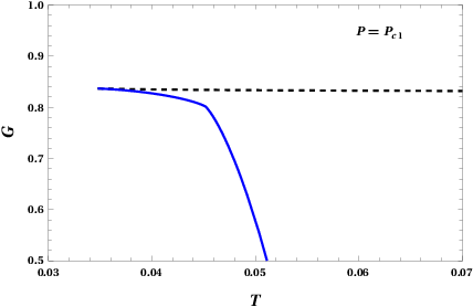
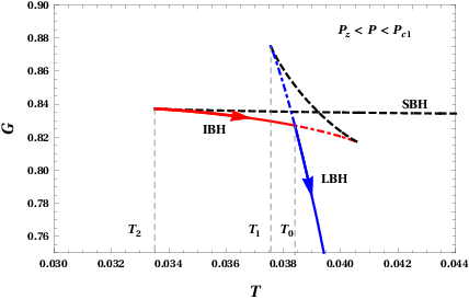
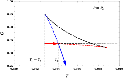
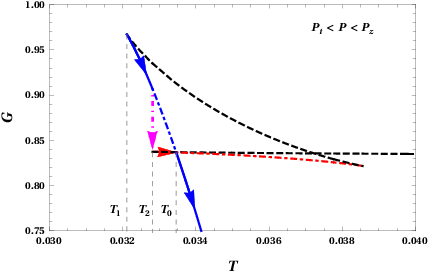
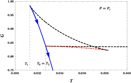
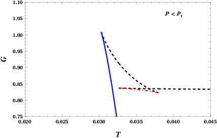
Now we focus on the reentrant phase transition exhibited by the BI-AdS black hole. Among the two cases of reentrant phase transition (case 2 and case 3), we chose case 3 in this article to demonstrate the associated properties. The results obtained are applicable for the case 2 of also. The reentrant phase transition can be better understood from Gibbs free energy study, as shown in Fig. 3. In the plots, for pressure , which corresponds to the second-order phase transition point, there is no swallow tail behaviour, as seen from Fig. 3. The solid blue line represents a stable phase of the system (LBH) with positive specific heat at constant pressure , while the dashed black line stands for unstable phase (SBH) of the system with negative . We emphasise the fact that SBH phase in RPT case is always unstable. There is no phase transition above the critical pressure . For pressures , we begin to observe a first-order phase transition, the indication being the swallowtail, Fig. 3. Here, we identify three temperatures, designated as , and . The points in the curve corresponding to and correspondingly connect the stable LBH (blue line) and stable IBH (red line) branches to unstable branches (dashed black). The temperature , which is the intersection of the stable IBH and LBH branches, is the point where a vdW like IBH-LBH first-order phase transition occurs. As we decrease the pressure, the mere first-order phase transition situation continues till , where we have , which is depicted in Fig 3. Further decreasing the pressure, , leads to a scenario where an additional zeroth-order phase transition is also exhibited by the system, Fig 3. This happens for a range of pressures , with . For a fixed pressure in this range, if the system is at some temperature initially, then it stays in LBH phase as the temperature increases, till . At temperature , the system finds a stable branch with lower Gibbs energy and jumps into the IBH phase. Unlike a first-order phase transition, there is a finite change in Gibbs free energy during this transition. Further, the system undergoes a secondary phase transition at from IBH to LBH phase, which is a first-order transition. In effect, the system undergoes LBH/IBH/LBH phase transition, the initial and final phases being the same. This is termed as a reentrant phase transition. This phenomenon disappears at , with , where the system has only LBH phase, Fig 3. There is no zeroth order or vdW like first-order phase transitions possible for the pressures , Fig. 3, wherein only the LBH phase exists. In short, the system exhibits both first order and zeroth-order phase transition for the range of pressures and temperatures , whereas only first-order phase transition for and .
The phase diagrams of the black hole corresponding to the reentrant phase transition case is presented in Fig. 4. As in SPT case, here also the results are obtained numerically by observing the behaviour of Gibbs free energy. Interestingly, for all values of pressure, we find that there is a lowest temperature below which there is no existence of black hole. The line which separates the black hole solutions from no black hole region is obtained by noting the temperature for pressures and for from the Gibbs free energy plots (Fig. 3). The result is shown in 4, where the separation line (black solid curve) has a discontinuity at . In the same plot, the transition lines of zeroth-order and first-order phase transition are also given. As is the zeroth-order phase transition point in the pressure range , the corresponding transition line (solid magenta line) matches with the extension of no black hole line from to . The first order coexistence line (red solid line) is also obtained from the Gibbs free energy behaviour. The first order coexistence curve and zeroth-order transition line meet at , which is the triple point. The zeroth order transition line terminates at , and the other at the critical point .
| 0.43 | 0.44 | 0.45 | 0.46 | 0.47 | 0.48 | 0.49 | |
|---|---|---|---|---|---|---|---|
| -0.000663 | -0.00186 | -0.003253 | -0.004888 | -0.006838 | -0.009242 | -0.012447 | |
| 0.033189 | 0.030199 | 0.026885 | 0.023198 | 0.019061 | 0.014328 | 0.008676 | |
| 0.003711 | 0.003686 | 0.003663 | 0.003643 | 0.003625 | 0.003609 | 0.003594 | |
| 0.045414 | 0.045289 | 0.045176 | 0.045074 | 0.044981 | 0.044895 | 0.044817 | |
| 0.002225 | 0.001922 | 0.001612 | 0.001294 | 0.000971 | 0.000644 | 0.000318 | |
| 0.037435 | 0.035249 | 0.032722 | 0.029762 | 0.026208 | 0.021759 | 0.015646 | |
| 0.002395 | 0.002101 | 0.00179 | 0.001464 | 0.001122 | 0.000747 | 0.000357 | |
| 0.037658 | 0.035457 | 0.032906 | 0.029914 | 0.026322 | 0.021821 | 0.015663 |
Here too we obtain the spinodal curves using the definition Eq. 25, which are shown in Fig. 4 along with the transition lines. The spinodal curve, the extremal points of the isothermal and isobaric curves by definition, have two turning points in the reentrant case, which are marked as and . As mentioned earlier, in case 3, which we have chosen, the point lies in the negative pressure region. The region between and is enlarged in Fig. 4. Note that, for the spinodal curve and no black hole line are the same. The regions separated by first-order coexistence line and zeroth-order transition line are clearly seen here. As both zeroth-order and first-order transitions are between IBH and LBH both lines separate these two phases in their respective domains. In Fig. 4, the phase structure for the reentrant case is given in plane, where the coexistence region of IBH and LBH is clearly shown. The IBH region is on the left, and the LBH is on the right side of the coexistence curve. As in plane here also the spinodal curve has two turning points, at the critical points and . In contrast to the case of SPT, here, the spinodal curve does not intersect the axis near the origin, instead shoots to infinity. On the other side, near the LBH phase, there is no change in the behaviour. The region near the origin is enlarged in the inset, where it can be seen that the IBH branch terminates when it meets the spinodal curve. Before concluding this section we list the values of , , and for different values for the reentrant case in table 2.
III Ruppeiner Geometry and Microstructure of the Black Hole
In this section, we investigate the microstructure of four-dimensional Born-Infeld AdS black hole using Ruppeiner geometry, constructed in the parameter space with fluctuation coordinates as temperature and volume. Particularly, we are interested in the microstructure that leads to the reentrant phase transition. As we will see, the underlying microstructure for the SPT has similarity with the RN-AdS black hole phase transition, whereas the RPT emerges due to a different nature of the black hole microstructure.
To set up the Ruppeiner geometry, we consider two subsystems of an isolated thermodynamic system having a total entropy . The smaller subsystem is assigned with an entropy and the larger subsystem with entropy . Viewing the larger subsystem as a thermal bath, we can take . Therefore, if the system is described by a set of independent variables and ,
| (26) |
When the system is in thermal equilibrium, the entropy is in its local maximum . Taylor expanding the entropy in the neighbourhood of the local maximum , we obtain
| (27) |
Since the first derivatives vanish for the equilibrium condition, we have
| (28) |
where we have truncated the higher order terms and the second term. The second term is negligible compared to the first term, as the entropy of the thermal bath is close to that of the whole system, and its second derivative with respect to the intensive variables are smaller than those of .
In Ruppeiner geometry, the entropy is taken as the thermodynamical potential and its fluctuation is related to the line element , which is the measure of the distance between two neighbouring fluctuation states of the thermodynamic system (Ruppeiner95). The Ruppeiner line element is given by,
| (29) |
where is the Boltzmann constant and the metric is,
| (30) |


Since the line element is related to the distance between the neighbouring fluctuation states, the metric must be encoded with the microscopic details of the system. Taking the fluctuation coordinates as temperature and volume, and Helmholtz free energy of the system as the thermodynamic potential, the line element can be shown to have the following form (Wei2019a),
| (31) |
where is the heat capacity at constant volume,
| (32) |


The Ruppeiner curvature scalar can be obtained directly from Eq. 31 by using the conventional definitions of Riemannian geometry. The curvature scalar so calculated is encoded with the interaction details of the microstructure of the system. The positive sign and negative sign are associated with repulsive and attractive interaction, respectively. If the Ruppeiner curvature vanishes, it implies that there is no effective interaction between the microscopic molecules. Moreover, the idea is that the Ruppeiner scalar diverges at the critical point. However, the Ruppeiner scalar obtained from the line element (31) has pathologies as the heat capacity vanishes for a spherically symmetric AdS black hole system. This in turn arises from the interdependence of the thermodynamic variables, namely entropy and volume. To overcome this issue, a normalised Ruppeiner scalar is defined as (Wei2019a),
| (33) |
where is the curvature scalar calculated from Eq. 31. The normalised curvature scalar diverges at the critical point of phase transition. Before proceeding further, we reiterate the following.
- •
The sign of reveals the nature of dominant interaction in the black hole microstructure. Positive/negative for repulsive/attractive and zero for no interaction.
- •
The absolute value of is the measure of the average number of correlated constituents, in general. For a black hole system, this could be the average number of correlated black hole molecules.
III.1 Standard Phase Transition Case
| 0.6 | 0.7 | 0.8 | 0.9 | 1 | |
|---|---|---|---|---|---|
| (CSSBH) | 2.06414 | 2.06982 | 2.073 | 2.07496 | 2.07629 |
| (CSSBH) | 2.57849 | 2.6243 | 2.64994 | 2.66583 | 2.67658 |
| (CSLBH) | 1.9239 | 1.9215 | 1.92011 | 1.91926 | 1.91868 |
| (CSLBH) | 1.49737 | 1.47446 | 1.46131 | 1.45317 | 1.44762 |
We obtained the normalised curvature scalar for the four-dimensional Born-Infeld AdS black hole using the above definitions. The SPT and RPT cases are analysed separately. The curvature scalar is expressed in terms of reduced parameters using Eq. 22 and Eq. 23 in the respective cases. First, we will analyse the SPT case. It is found that the behaviour of for SPT case is similar to that of RN-AdS black hole. The functional behaviour of against thermodynamic volume for a fixed temperature of is studied in fig. (5). For , below critical temperature, has two negative divergences. These two divergences gradually come closer as temperature increases and merge at . The divergence at critical temperature occurs at . For temperatures above the critical value, both divergences disappear. The divergences of are related to the spinodal curve. In fact, diverges along the spinodal curve. Since is doubly degenerate in the spinodal curve (Fig. 2), below critical point, it leads to two divergences for . For low temperatures, we notice that takes positive values in a very small domain (shown in the insets of Fig. 8, near the origin) as , which is the small black hole phase. We observe positive on both sides of the near origin divergence. The left side corresponds to the SBH phase (shaded yellow) and the right side corresponds to the coexistence phase (shaded green). The shaded yellow region exists for all temperatures , whereas the shaded green region disappears after a particular . This can be understood clearly using the sign-changing curve later (Fig. 6). The yellow region implies that the SBH phase has a dominant repulsive interaction. On the other hand, the LBH phase is always characterised by the dominant attractive interaction. To check whether the repulsive interaction regions are thermodynamically stable, we present the regions of with different sign in plane along with the coexistence and the spinodal curves (fig. 6). The sign-changing curve of is obtained by setting . The solution satisfy the condition , where is the sign-changing temperature and temperature along the spinodal curve. In fig. 6, the shaded region corresponds to the negative sign of . Region is the coexistence region of SBH and LBH. Region lies in the metastable phase, which is not interesting from the thermodynamic perspective. Region includes part of SBH phase of the black hole, implying repulsive interactions among the small black hole constituents.


We now examine the behaviour of along the coexistence curve and study the critical phenomena 6. The nature of interaction can be better understood from the behaviour of along the coexistence curve. From Fig. 6 it is clear that LBH phase always has dominant attractive interaction ( always negative), whereas, the SBH phase switches to dominant repulsive interaction ( positive) from dominant attractive interaction ( negative) for low temperature values. The analysis for different values of Born Infeld parameter in the SPT range was performed numerically. In the reduced coordinates, when the type of interaction in SBH switches between attractive and repulsive interaction, for the corresponding temperatures are . For temperatures above these, the absolute value of the curvature scalar of the LBH is greater than that of the SBH. This implies that the attractive interaction in the LBH is stronger than SBH. Both the SBH and LBH branches diverge to negative infinity at the critical point. This can be seen as being due to the divergence of correlation length at the critical point. This is a universal behaviour observed in other black hole systems in AdS spacetime. We obtain the critical exponent of the normalised scalar curvature at the critical point. Since the analytical expansion is not feasible, we assume that the scalar curvature has the following form near the critical point,
| (34) |
Taking logarithm on both sides,
| (35) |
Along the coexistence curve, for and we obtained,
| (36) |
for the SBH branch and,
| (37) |
for the LBH branch. These are shown in Fig. 7. Considering the numerical errors we have the critical exponent . Averaging the values, we have,
| (38) |
From the numerical results given in table 3, we have,
| (39) |
for , respectively. These values are slightly more negative than . Our results are in agreement with that of both the charged AdS black hole and vdW fluid, which have a with a critical exponent of and constant value of for , near the critical point, which is a universal behaviour.
To summarise the nature of interaction in the underlying microstructure of SPT, the LBH phase is always characterised by attractive interaction (like a bosonic gas), whereas, the SBH phase can have both attractive and repulsive interaction (like a quantum anyon gas).


III.2 Reentrant Phase Transition Case
We analyse the underlying microstructure of the black hole that results in RPT using the same method as before. The normalised Ruppeiner curvature scalar is plotted against the volume for constant temperatures in Fig. 8. Compared to the SPT case, here we observe an additional divergence for all temperatures , and only one divergence for . This is because, the spinodal curve has a different structure in the RPT case (Fig. 2) compared to SPT case (Fig. 4). For phase transition temperatures, which lie in the range , there exist three divergences as shown in Fig 8 and Fig. 8. Most general conclusions on the appearance of this divergences can be learnt from the spinodal curve. Here, the left-most divergence, say , corresponds to the spinodal curve branch that shoots to infinity after turning from in Fig. 4, which exists for temperatures . The middle divergence, say , corresponds to the spinodal curve between and , appearing in the temperature range . And the rightmost divergence, say , is on the spinodal curve on the LBH side after , which present for all temperatures . At divergences and merge together at , leaving only in total two divergences, Fig. 8. For completeness we mention that, at divergences and merge together, which is not relevant and hence not shown here. Interestingly, one divergence remains even for temperatures , Fig. 8. These divergences separate different phases of the black hole from each other in the plane, which enables us to search for the kind of interaction in each phase. The region between and corresponds to IBH phase and right side of to LBH phase. Left side of , and between and are coexistence regions. Contrary to the SPT case, always takes negative values, implying only a dominant attractive interaction in all of the phases in RPT case. We search for a possible repulsive interaction at low values, shown in the inset of Fig. 8, which is a null result. This result is true for all phase transition temperatures. In short, for RPT case the black hole microstructure has only attractive interactions.


| 0.43 | 0.44 | 0.45 | 0.46 | 0.47 | 0.48 | 0.49 | |
|---|---|---|---|---|---|---|---|
| (CSIBH) | 1.91582 | 2.01262 | 2.07636 | 1.99898 | 2.02411 | 2.03111 | 2.03868 |
| (CSIBH) | 1.68789 | 2.2181 | 2.56921 | 2.17032 | 2.31204 | 2.357 | 2.40382 |
| (CSLBH) | 2.04466 | 1.9619 | 1.91492 | 1.99174 | 1.95724 | 1.9511 | 1.94448 |
| (CSLBH) | 2.19809 | 1.75127 | 1.49509 | 1.8951 | 1.70734 | 1.67 | 1.63093 |
We confirm the above result by looking at the region covered by the sign-changing curve (Fig. 9). The positive values, shaded region, do not overlap with any stable state of the system. Note that the transition line of the zeroth-order phase transition (solid magenta line) also lies outside the shaded region. Near origin domain is enlarged in the inset for clarity. The behaviour of along the transition curve is analysed in Fig. 9. We consider the first-order phase transition coexistence curve and the zeroth-order transition curve. As the zeroth-order transition line is not a coexistence curve, it gives only one branch. We consider only the region of temperature where the phase transition takes place, , as below the temperature there is no phase transition. Once again, the positive sign of asserts that, both IBH and LBH phases have dominant attractive interaction (like a bosonic gas). That is, during a reentrant phase transition in BI-AdS black hole, both the zeroth-order and first-order transition preserve the nature of the interaction between the microstructures. However, we notice that the correlation between the constituents changes at different temperatures. The flipping temperatures are clearly shown in Fig. 9 in blue dots. For zeroth-order transition (jumping from blue dashed line to magenta dot-dashed line and vice versa), IBH phase has higher correlation strength than LBH in the temperature range . This property is reversed in the region . On the other hand, for the first-order phase transition (jumping from blue dashed line to red solid line and vice versa), IBH phase exhibits higher correlation among the constituents than LBH for temperatures , which is flipped for . In fact, the change in the strength of the interaction is also present in SPT case. Interestingly, near the triple point, IBH phase shows a huge surge in correlation, whereas the correlation in LBH phase here, is very weak. Also, the red and magenta line merge near , signifying the meeting and termination of zeroth-order and first-order transition line at that point. As in SPT case near the critical point the diverging correlation length leads to diverging . For magenta line it happens at , in a sense acts as a critical point (see for example (Altamirano:2013ane)). During a RPT, the initial and final phases are the same from the macroscopic point of view. Microscopically, this is almost true for , where red and magenta line (initial and final states in RPT) are close together. However, for there is a difference in strength of interaction, which becomes considerable near .
The critical phenomena of is studied for different values of numerically using Eq. 34. From the numerical results given in table 4, we have,
| (40) |
for , respectively. As in the case of SPT, these values are slightly more negative than . Within the numerical errors we have obtained the universal constant as and the critical exponent in RPT case too. To cut a long story short, we observe the existence of only homogeneous dominant attractive interaction in the black hole for RPT case, and both repulsive and attractive interaction in SPT case. This difference in the microstructure interaction for SPT and RPT in BI-AdS black hole tells that the microstructure is determined by the coupling parameter .
IV Discussions
In this article, we have studied the microstructure of four-dimensional Born-Infeld AdS black hole employing a novel Ruppeiner geometry method. As the entropy and volume are interdependent in a spherically symmetric AdS black hole, the application of Ruppeiner geometry for such a system must be carried out with utmost care. Keeping this in mind, we have constructed the Ruppeiner curvature scalar in the parametric space where the temperature and volume are the fluctuation coordinates. We investigated the phase structure and the corresponding microscopic interactions for both the standard van der Waals (SPT) and the reentrant phase transitions (RPT), where a first-order phase transition is accompanied by a zeroth-order transition. We found that the microstructure that leads to RPT is distinct from that of SPT. Our study shows that the Born Infeld coupling coefficient determines the microscopic interaction of the black hole. Since the analytical investigation is not possible due to the complexity of the spacetime, we have carried out the study numerically.
In the first part of the article, we investigated the phase structure of the black hole using the spinodal and transition curves in SPT and RPT cases. The black hole has four different cases depending on the value of , and shows the distinct RPT for certain pressure range. There are two RPT cases with two critical points in each. It is found that the phase structure associated with SPT and RPT are distinct. The phase diagrams are presented in pressure-temperature () and temperature-volume () planes, where, stable, metastable and coexistence phases are studied. In both SPT and RPT cases, we conveniently define the reduced parameters and all analyses were carried out in terms of them.
The second half of the article is devoted to the study of microstructure, which reveal distinct microstructure for SPT and RPT cases. Two important features, the nature of interaction and strength of correlation are sought for in this study. The microstructure that corresponds to SPT is analogous to that of RN-AdS black hole. The small black hole phase shows a dominant repulsive interaction in a certain range of parameters. As the interaction in this phase is attractive in other domains of parameter space, the interaction type resembles that of a quantum anyon gas. The large black hole phase is always characterised by the dominant attractive interaction, like a bosonic gas. These are inferred from the sign of the Ruppeiner curvature scalar . For both small black hole and large black hole branches, it diverges near the critical point. The RPT case has a different microstructure compared to the SPT case, wherein no repulsive interaction is present for both the intermediate and large black hole phases. The nature of microstructure does not change during the zeroth-order and first-order phase transition in RPT, which as a dominant attractive interaction. This suggests that the nature of interaction in RPT case is always like that of a bosonic gas. Both, intermediate and large black hole, branches diverge near the physically meaningful critical point. The signature of RPT is reflected in the behaviour of curvature scalar, through its anomalies near the termination points of the zeroth-order phase transition. The strength of interaction depends on temperature, which is inferred from the magnitude of the curvature scalar, the high correlation phases are flipped at certain temperatures for both zeroth-order and first-order transition. In fact, this reversal of correlation strength is true for SPT case too. The critical phenomenon of the system is investigated via curvature scalar. The universal properties, critical exponent- and the constant , are obtained for SPT and RPT cases over a range of values. We believe that this study will help us shed more light on the black hole microstructure in general.
Acknowledgements.
Authors N.K.A., A.R.C.L. and K.H. would like to thank U.G.C. Govt. of India for financial assistance under UGC-NET-SRF scheme. M.S.A.’s research is supported by the ISIRD grant 9-252/2016/IITRPR/708.References
- (1) S. W. Hawking, Particle Creation by Black Holes, Commun. Math. Phys. 43 (1975) 199.
- (2) J. D. Bekenstein, Black holes and the second law, Lett. Nuovo Cim. 4 (1972) 737.
- (3) J. D. Bekenstein, Black holes and entropy, Phys. Rev. D7 (1973) 2333.
- (4) J. M. Bardeen, B. Carter and S. W. Hawking, The Four laws of black hole mechanics, Commun. Math. Phys. 31 (1973) 161.
- (5) D. Kastor, S. Ray and J. Traschen, Enthalpy and the Mechanics of AdS Black Holes, Class. Quant. Grav. 26 (2009) 195011 [0904.2765].
- (6) B. P. Dolan, Pressure and volume in the first law of black hole thermodynamics, Class. Quant. Grav. 28 (2011) 235017 [1106.6260].
- (7) D. Kubiznak and R. B. Mann, P-V criticality of charged AdS black holes, JHEP 07 (2012) 033 [1205.0559].
- (8) S. Gunasekaran, R. B. Mann and D. Kubiznak, Extended phase space thermodynamics for charged and rotating black holes and Born-Infeld vacuum polarization, JHEP 11 (2012) 110 [1208.6251].
- (9) D. Kubiznak, R. B. Mann and M. Teo, Black hole chemistry: thermodynamics with Lambda, Class. Quant. Grav. 34 (2017) 063001 [1608.06147].
- (10) C. S. Hudson, Die gegenseitige löslichkeit von nikotin in wasser, Zeitschrift für Physikalische Chemie 47 (1904) 113.
- (11) T. Narayanan and A. Kumar, Reentrant phase transitions in multicomponent liquid mixtures, physrep 249 (1994) 135.
- (12) O. Panella and P. Roy, Re-entrant phase transitions in non-commutative quantum mechanics, in Journal of Physics Conference Series, vol. 670 of Journal of Physics Conference Series, p. 012040, Jan., 2016, DOI.
- (13) D.-C. Zou, S.-J. Zhang and B. Wang, Critical behavior of Born-Infeld AdS black holes in the extended phase space thermodynamics, Phys. Rev. D 89 (2014) 044002 [1311.7299].
- (14) N. Altamirano, D. Kubiznak and R. B. Mann, Reentrant phase transitions in rotating anti–de Sitter black holes, Phys. Rev. D 88 (2013) 101502 [1306.5756].
- (15) N. Altamirano, D. Kubizˇnák, R. B. Mann and Z. Sherkatghanad, Kerr-AdS analogue of triple point and solid/liquid/gas phase transition, Class. Quant. Grav. 31 (2014) 042001 [1308.2672].
- (16) N. Altamirano, D. Kubiznak, R. B. Mann and Z. Sherkatghanad, Thermodynamics of rotating black holes and black rings: phase transitions and thermodynamic volume, Galaxies 2 (2014) 89 [1401.2586].
- (17) D. Kubiznak and F. Simovic, Thermodynamics of horizons: de Sitter black holes and reentrant phase transitions, Class. Quant. Grav. 33 (2016) 245001 [1507.08630].
- (18) A. M. Frassino, D. Kubiznak, R. B. Mann and F. Simovic, Multiple Reentrant Phase Transitions and Triple Points in Lovelock Thermodynamics, JHEP 09 (2014) 080 [1406.7015].
- (19) S.-W. Wei and Y.-X. Liu, Triple points and phase diagrams in the extended phase space of charged Gauss-Bonnet black holes in AdS space, Phys. Rev. D 90 (2014) 044057 [1402.2837].
- (20) R. A. Hennigar, W. G. Brenna and R. B. Mann, criticality in quasitopological gravity, JHEP 07 (2015) 077 [1505.05517].
- (21) Z. Sherkatghanad, B. Mirza, Z. Mirzaiyan and S. A. Hosseini Mansoori, Critical behaviors and phase transitions of black holes in higher order gravities and extended phase spaces, Int. J. Mod. Phys. D 26 (2016) 1750017 [1412.5028].
- (22) R. A. Hennigar and R. B. Mann, Reentrant phase transitions and van der Waals behaviour for hairy black holes, Entropy 17 (2015) 8056 [1509.06798].
- (23) A. Dehyadegari and A. Sheykhi, Reentrant phase transition of Born-Infeld-AdS black holes, Phys. Rev. D 98 (2018) 024011 [1711.01151].
- (24) Y.-M. Xu, H.-M. Wang, Y.-X. Liu and S.-W. Wei, Photon sphere and reentrant phase transition of charged Born-Infeld-AdS black holes, Phys. Rev. D 100 (2019) 104044 [1906.03334].
- (25) F. Weinhold, Metric geometry of equilibrium thermodynamics, The Journal of Chemical Physics 63 (1975) 2479 [https://doi.org/10.1063/1.431689].
- (26) G. Ruppeiner, Riemannian geometry in thermodynamic fluctuation theory, Rev. Mod. Phys. 67 (1995) 605.
- (27) G. Ruppeiner, Thermodynamics: A riemannian geometric model, Phys. Rev. A 20 (1979) 1608.
- (28) H. Janyszek, Riemannian geometry and stability of thermodynamical equilibrium systems, Journal of Physics A Mathematical General 23 (1990) 477.
- (29) G. Ruppeiner, Application of riemannian geometry to the thermodynamics of a simple fluctuating magnetic system, Phys. Rev. A 24 (1981) 488.
- (30) H. Janyszek and R. Mrugal/a, Riemannian geometry and the thermodynamics of model magnetic systems, Phys. Rev. A 39 (1989) 6515.
- (31) H. Janyszek and R. Mrugaa, Riemannian geometry and stability of ideal quantum gases, Journal of Physics A: Mathematical and General 23 (1990) 467.
- (32) H. Oshima, T. Obata and H. Hara, Riemann scalar curvature of ideal quantum gases obeying gentile’s statistics, Journal of Physics A: Mathematical and General 32 (1999) 6373.
- (33) B. Mirza and H. Mohammadzadeh, Ruppeiner geometry of anyon gas, Phys. Rev. E 78 (2008) 021127.
- (34) H.-O. May, P. Mausbach and G. Ruppeiner, Thermodynamic curvature for attractive and repulsive intermolecular forces, Phys. Rev. E 88 (2013) 032123.
- (35) G. Ruppeiner, Thermodynamic curvature and black holes, Springer Proc. Phys. 153 (2014) 179 [1309.0901].
- (36) R.-G. Cai and J.-H. Cho, Thermodynamic curvature of the BTZ black hole, Phys. Rev. D 60 (1999) 067502 [hep-th/9803261].
- (37) J. E. Aman, I. Bengtsson and N. Pidokrajt, Geometry of black hole thermodynamics, Gen. Rel. Grav. 35 (2003) 1733 [gr-qc/0304015].
- (38) B. Mirza and M. Zamani-Nasab, Ruppeiner Geometry of RN Black Holes: Flat or Curved?, JHEP 06 (2007) 059 [0706.3450].
- (39) A. Sahay, T. Sarkar and G. Sengupta, Thermodynamic Geometry and Phase Transitions in Kerr-Newman-AdS Black Holes, JHEP 04 (2010) 118 [1002.2538].
- (40) P. Chaturvedi, A. Das and G. Sengupta, Thermodynamic Geometry and Phase Transitions of Dyonic Charged AdS Black Holes, Eur. Phys. J. C 77 (2017) 110 [1412.3880].
- (41) S.-W. Wei, B. Liang and Y.-X. Liu, Critical phenomena and chemical potential of a charged AdS black hole, Phys. Rev. D 96 (2017) 124018 [1705.08596].
- (42) P. Chaturvedi, S. Mondal and G. Sengupta, Thermodynamic Geometry of Black Holes in the Canonical Ensemble, Phys. Rev. D 98 (2018) 086016 [1705.05002].
- (43) H. Quevedo, Geometrothermodynamics, J. Math. Phys. 48 (2007) 013506 [physics/0604164].
- (44) H. Liu, H. Lu, M. Luo and K.-N. Shao, Thermodynamical Metrics and Black Hole Phase Transitions, JHEP 12 (2010) 054 [1008.4482].
- (45) C. Niu, Y. Tian and X.-N. Wu, Critical Phenomena and Thermodynamic Geometry of RN-AdS Black Holes, Phys. Rev. D 85 (2012) 024017 [1104.3066].
- (46) S.-W. Wei and Y.-X. Liu, Critical phenomena and thermodynamic geometry of charged Gauss-Bonnet AdS black holes, Phys. Rev. D 87 (2013) 044014 [1209.1707].
- (47) R. Banerjee and D. Roychowdhury, Critical phenomena in Born-Infeld AdS black holes, Phys. Rev. D 85 (2012) 044040 [1111.0147].
- (48) S. A. H. Mansoori and B. Mirza, Correspondence of phase transition points and singularities of thermodynamic geometry of black holes, Eur. Phys. J. C 74 (2014) 2681 [1308.1543].
- (49) J.-X. Mo, X.-X. Zeng, G.-Q. Li, X. Jiang and W.-B. Liu, A unified phase transition picture of the charged topological black hole in Horava-Lifshitz gravity, JHEP 10 (2013) 056 [1404.2497].
- (50) S. A. H. Mansoori, B. Mirza and M. Fazel, Hessian matrix, specific heats, Nambu brackets, and thermodynamic geometry, JHEP 04 (2015) 115 [1411.2582].
- (51) S. H. Hendi and R. Naderi, Geometrothermodynamics of black holes in Lovelock gravity with a nonlinear electrodynamics, Phys. Rev. D 91 (2015) 024007 [1510.06269].
- (52) B. P. Dolan, Intrinsic curvature of thermodynamic potentials for black holes with critical points, Phys. Rev. D 92 (2015) 044013 [1504.02951].
- (53) S. A. H. Mansoori, B. Mirza and E. Sharifian, Extrinsic and intrinsic curvatures in thermodynamic geometry, Phys. Lett. B 759 (2016) 298 [1602.03066].
- (54) S. A. Hosseini Mansoori and B. Mirza, Geometrothermodynamics as a singular conformal thermodynamic geometry, Phys. Lett. B 799 (2019) 135040 [1905.01733].
- (55) R. Banerjee, S. Ghosh and D. Roychowdhury, New type of phase transition in Reissner Nordström–AdS black hole and its thermodynamic geometry, Phys. Lett. B 696 (2011) 156 [1008.2644].
- (56) R. Banerjee, S. K. Modak and S. Samanta, Second Order Phase Transition and Thermodynamic Geometry in Kerr-AdS Black Hole, Phys. Rev. D 84 (2011) 064024 [1005.4832].
- (57) S.-W. Wei and Y.-X. Liu, Insight into the Microscopic Structure of an AdS Black Hole from a Thermodynamical Phase Transition, Phys. Rev. Lett. 115 (2015) 111302 [1502.00386].
- (58) X.-Y. Guo, H.-F. Li, L.-C. Zhang and R. Zhao, Microstructure and continuous phase transition of a Reissner-Nordstrom-AdS black hole, Phys. Rev. D100 (2019) 064036 [1901.04703].
- (59) Y.-Z. Du, R. Zhao and L.-C. Zhang, Microstructure and Continuous Phase Transition of the Gauss-Bonnet AdS Black Hole, 1901.07932.
- (60) A. Dehyadegari, A. Sheykhi and A. Montakhab, Critical behavior and microscopic structure of charged AdS black holes via an alternative phase space, Phys. Lett. B768 (2017) 235 [1607.05333].
- (61) M. Chabab, H. El Moumni, S. Iraoui, K. Masmar and S. Zhizeh, More Insight into Microscopic Properties of RN-AdS Black Hole Surrounded by Quintessence via an Alternative Extended Phase Space, Int. J. Geom. Meth. Mod. Phys. 15 (2018) 1850171 [1704.07720].
- (62) G.-M. Deng and Y.-C. Huang, - criticality and microstructure of charged AdS black holes in gravity, Int. J. Mod. Phys. A32 (2017) 1750204 [1705.04923].
- (63) M. Kord Zangeneh, A. Dehyadegari, A. Sheykhi and R. B. Mann, Microscopic Origin of Black Hole Reentrant Phase Transitions, Phys. Rev. D97 (2018) 084054 [1709.04432].
- (64) Y.-G. Miao and Z.-M. Xu, On thermal molecular potential among micromolecules in charged AdS black holes, Phys. Rev. D98 (2018) 044001 [1712.00545].
- (65) Y.-G. Miao and Z.-M. Xu, Microscopic structures and thermal stability of black holes conformally coupled to scalar fields in five dimensions, Nucl. Phys. B942 (2019) 205 [1711.01757].
- (66) Y. Chen, H. Li and S.-J. Zhang, Microscopic explanation for black hole phase transitions via Ruppeiner geometry: Two competing factors–the temperature and repulsive interaction among BH molecules, Nucl. Phys. B948 (2019) 114752 [1812.11765].
- (67) Z.-M. Xu, B. Wu and W.-L. Yang, The fine micro-thermal structures for the Reissner-Nordström black hole, 1910.03378.
- (68) A. N. Kumara, C. L. A. Rizwan, D. Vaid and K. M. Ajith, Critical Behaviour and Microscopic Structure of Charged AdS Black Hole with a Global Monopole in Extended and Alternate Phase Spaces, 1906.11550.
- (69) A. N. Kumara, C. L. A. Rizwan, K. Hegde, A. K. M. and M. S. Ali, Microstructure and continuous phase transition of a regular Hayward black hole in anti-de Sitter spacetime, 2003.00889.
- (70) S.-W. Wei, Y.-X. Liu and R. B. Mann, Repulsive Interactions and Universal Properties of Charged Anti–de Sitter Black Hole Microstructures, Phys. Rev. Lett. 123 (2019) 071103 [1906.10840].
- (71) S.-W. Wei, Y.-X. Liu and R. B. Mann, Ruppeiner Geometry, Phase Transitions, and the Microstructure of Charged AdS Black Holes, Phys. Rev. D100 (2019) 124033 [1909.03887].
- (72) S.-W. Wei and Y.-X. Liu, Intriguing microstructures of five-dimensional neutral Gauss-Bonnet AdS black hole, Phys. Lett. B803 (2020) 135287 [1910.04528].
- (73) A. Naveena Kumara, C. A. Rizwan, K. Hegde and A. K. M, Repulsive Interactions in the Microstructure of Regular Hayward Black Hole in Anti-de Sitter Spacetime, Phys. Lett. B807 (2020) 135556 [2003.10175].
- (74) S.-W. Wei and Y.-X. Liu, Extended thermodynamics and microstructures of four-dimensional charged Gauss-Bonnet black hole in AdS space, Phys. Rev. D 101 (2020) 104018 [2003.14275].
- (75) B. Wu, C. Wang, Z.-M. Xu and W.-L. Yang, Ruppeiner geometry and thermodynamic phase transition of the black hole in massive gravity, 2006.09021.
- (76) Z.-M. Xu, B. Wu and W.-L. Yang, Ruppeiner thermodynamic geometry for the Schwarzschild-AdS black hole, Phys. Rev. D 101 (2020) 024018 [1910.12182].
- (77) A. Ghosh and C. Bhamidipati, Thermodynamic geometry for charged Gauss-Bonnet black holes in AdS spacetimes, Phys. Rev. D101 (2020) 046005 [1911.06280].
- (78) A. Ghosh and C. Bhamidipati, Thermodynamic geometry and interacting microstructures of BTZ black holes, 2001.10510.
- (79) P. K. Yerra and C. Bhamidipati, Ruppeiner Geometry, Phase Transitions and Microstructures of Black Holes in Massive Gravity, 2006.07775.
- (80) A. Dehyadegari, A. Sheykhi and S.-W. Wei, Microstructure of charged AdS black hole via criticality, 2006.12265.
- (81) M. Born and L. Infeld, Foundations of the new field theory, Proc. Roy. Soc. Lond. A A144 (1934) 425.
- (82) G. W. Gibbons, Aspects of Born-Infeld theory and string / M theory, AIP Conf. Proc. 589 (2001) 324 [hep-th/0106059].
- (83) S. Fernando and D. Krug, Charged black hole solutions in Einstein-Born-Infeld gravity with a cosmological constant, Gen. Rel. Grav. 35 (2003) 129 [hep-th/0306120].
- (84) T. K. Dey, Born-Infeld black holes in the presence of a cosmological constant, Phys. Lett. B 595 (2004) 484 [hep-th/0406169].
- (85) R.-G. Cai, D.-W. Pang and A. Wang, Born-Infeld black holes in (A)dS spaces, Phys. Rev. D 70 (2004) 124034 [hep-th/0410158].