Two-photon-interaction effects in the bad-cavity limit
Abstract
Various experimental platforms have proven to be valid testbeds for the implementation of nondipolar light-matter interactions, where atomic systems and confined modes interact via two-photon couplings. Here, we study a damped quantum harmonic oscillator interacting with two-level systems via a two-photon coupling in the so-called bad-cavity limit, in the presence of finite-temperature baths and coherent and incoherent drivings. We have succeeded in applying a recently developed adiabatic elimination technique to derive an effective master equation for the two-level systems, presenting two fundamental differences compared to the case of a dipolar interaction: an enhancement of the two-level systems spontaneous-like emission rate, including a thermal contribution and a quadratic term in the coherent driving, and an increment of the effective temperature perceived by the two-level systems. These differences give rise to striking effects in the two-level systems dynamics, including a faster generation of steady-state coherence and a richer dependence on temperature of the collective effects, which can be made stronger at higher temperature.
I Introduction
Atomic systems interacting with confined photonic or phononic modes represent one of the most studied classes of quantum-optical systems. On the one hand, the confinement may induce modifications of single atom absorption and emission rates such as the well-known Purcell effect Haroche and Raimond 2006. On the other hand, the collective nature of such interactions gives rise to a rich quantum phenomenology characterized, for example, by the emergence of quantum phase transitions Kirton et al. 2019 and by the qualitative modifications of optical properties Benedict 1996. Concerning the latter, a sub and a superradiant regime have been identified, respectively characterized by the dampening or the amplification of atomic absorption and emission rates with respect to the independent-emitter case Gross and Haroche 1982. These regimes have been extensively studied also in the presence of coherent or incoherent optical drivings Meiser et al. 2009; Meiser and Holland 2010a; Meiser and Holland 2010b; Auffèves et al. 2011; Shammah et al. 2017; Kirton and Keeling 2018; Shammah et al. 2018; Damanet et al. 2019. Much attention has been devoted to the so-called bad-cavity limit in which the confined mode is strongly dampened with respect to the interaction with the atoms Meiser et al. 2009; Meiser and Holland 2010a; Meiser and Holland 2010b; Auffèves et al. 2011; Kirton and Keeling 2018; Shammah et al. 2018. In this context, the effective dynamics of the atoms can be obtained by adiabatically eliminating the confined mode Bonifacio et al. 1971a; Bonifacio et al. 1971b; Azouit et al. 2017; Azouit 2017.
Besides the fundamental interest, collective quantum phenomena induced by light-matter interactions can be exploited in a variety of applications. In particular, the sub and superradiant regimes may be associated to the generation of collective states of the emitters, which are of great interest for quantum sensing Leroux et al. 2010; Tóth and Apellaniz 2014, generation of nonclassical states Jahnke et al. 2016, photon storage Asenjo-Garcia et al. 2017, and excitation transfer Garcia-Vidal and Feist 2017. This phenomenology is of high experimental relevance, as collective light-matter interactions can be controllably implemented in a broad range of atomic and solid-state quantum systems, such as cold atoms Goban et al. 2015, trapped ions DeVoe and Brewer 1996, metamaterials Jenkins et al. 2017, plasmonic cavities Pustovit and Shahbazyan 2009, color centres in diamonds Angerer et al. 2018, quantum dots Scheibner et al. 2007, and superconducting circuits Mlynek et al. 2014.
To the best of our knowledge, collective radiative phenomena have not so far been analyzed for two-photon (2ph) interactions. However, it has been recently predicted that using atomic or solid-state systems it is possible to implement nondipolar light-matter couplings, where the linear interaction is inhibited and where quantum emitters and localized bosonic modes interact via the exchange of two excitation quanta. In particular, such two-photon couplings can be observed by engineering superconducting atom-resonator systems Felicetti et al. 2018a; Felicetti et al. 2018b or by applying analog quantum simulation schemes in trapped-ions Felicetti et al. 2015; Cheng et al. 2018; Puebla et al. 2019 or ultracold atoms Schneeweiss et al. 2018; Dareau et al. 2018. Notice that nondipolar transitions have already been observed using superconducting artificial atoms Goetz et al. 2018, and that quantum-simulation techniques have already been experimentally applied to observe the physics of fundamental dipolar light-matter interaction models in extreme regimes of parameters Dareau et al. 2018; Lv et al. 2018. On the dissipative side, two-photon relaxation Minganti et al. 2016; Malekakhlagh and Rodriguez 2019 and pumping Minganti et al. 2016 have also been theoretically analyzed and experimentally implemented Leghtas et al. 2015. The fast-growing interest in two-photon couplings is motivated by a rich phenomenology, characterized by counter-intuitive spectral features Travěnec 2012; Duan et al. 2016; Maciejewski and Stachowiak 2017; Xie et al. 2019; Cong et al. 2019; Armenta Rico et al. 2020, high-order quantum optical nonlinearities Felicetti et al. 2018a; Felicetti et al. 2018b; Zou et al. 2020, and quantum phase transitions Garbe et al. 2017; Chen and Zhang 2018; Cui et al. 2019; Garbe et al. 2019; Cui et al. 2020. In turn, this phenomenology can be exploited in different quantum-information applications Villas-Boas and Rossatto 2019; Casanova et al. 2018; González-Gutiérrez and Torres 2019. We finally stress that the two-photon coupling analyzed here differs from other physical situations for which the term “two-photon” is used. Some examples are: two-photon excitations (see chapter 6.7 of Ref. Loudon 2000), two-photon absorption Rumi and Perry 2010, two-plasmon emission Rivera et al. 2016, and two-photon emission coming from strong light-matter coupling Flick et al. 2018.
In this Letter, we study the dynamics of a damped harmonic oscillator (HO) interacting with an ensemble of two-level systems (TLSs) in the bad-cavity limit in the case of a two-photon coupling. By applying a recently developed approach to perform adiabatic elimination in open quantum systems Azouit 2017; Azouit et al. 2017, we derive an effective master equation for the TLSs that takes into account the coupling with finite-temperature baths as well as coherent and incoherent optical drivings. Our analytical and numerical analysis of the time evolution and steady-state behavior unveils a unexpected collective phenomenology induced by nondipolar light-matter interactions. Compared to the dipolar case, the two-photon coupling introduces the possibility to enhance the absorption and emission processes, and leads to a higher resilience of sub- and superradiance with respect to the baths temperature.
II Physical models
We study a system composed of a damped HO interacting via a resonant Jaynes-Cummings Hamiltonian with TLSs in the bad-cavity limit Bonifacio et al. 1971a; Bonifacio et al. 1971b; Azouit 2017, comparing the one-photon (1ph) and 2ph interaction cases. The two models are described by the Hamiltonians
| (1) |
where for the 1ph case and for the 2ph one, is the frequency of the HO and the one of the TLSs (i.e., we consider a resonant interaction in both cases), is the coupling parameter between the HO and the TLSs, and are the usual annihilation and creation operators of a HO, while and , where , , and are, respectively, the -Pauli, the lowering, and the raising operators of a TLS. The ground and the excited energy levels of each TLS are indicated, respectively, by and . In Appendix A we provide an example of a possible implementation with superconducting circuits Blais et al. 2021 of the above Hamiltonian for the case , by generalizing the study done in Ref. Felicetti et al. 2018b to the case of more than one TLS.
We suppose that the HO and each TLS are each in contact with an independent thermal bath at temperature (equal for all baths) and that a resonant coherent pumping on the HO and an incoherent local pumping on the TLSs are available. In the interaction picture, using a phenomenological approach Breuer and Petruccione 2007; Rivas et al. 2010; Giorgi et al. 2020, the master equation for the global density matrix is
| (2) |
where and are dissipators acting, respectively, on the HO and on the TLSs, given by
| (3) |
where , and are the relaxation rates of, respectively, the HO and each TLS due to the local couplings with their own thermal baths ( is assumed to be the same for all the TLSs), characterizes the interaction between the HO and the coherent field, quantifies the action of the incoherent pumping on each TLS, and , being the Boltzmann constant. The coherent pumping is treated in the rotating-wave approximation, being . The phenomenological approach is justified because we consider the TLSs and the HO weakly coupled () Breuer and Petruccione 2007, the HO weakly coupled to its bath () Breuer and Petruccione 2007, and the external coherent field resonant with the HO Rivas et al. 2010.
III Adiabatic elimination
By applying a recently introduced adiabatic elimination technique Azouit 2017; Azouit et al. 2017 we have been able to derive an effective master equation for the reduced density matrix of the TLSs, (see Appendices B and C for a review of this technique, the detailed derivation, and some comments on the validity range of the adiabatic elimination):
| (4) |
where we recall that for the 1ph case and for the 2ph one, and
| (5) |
As expected, even in the 2ph case the adiabatic elimination gives rise to collective dissipative terms [second line of Eq. (III)]. We observe that differently from the case of collective radiative phenomena induced by the interaction of different atoms with a common vacuum field Gross and Haroche 1982, here the collective phenomena result from the coupling with a common damped HO. Notice that, although Eq. (III) retains its formal structure when changing (see Appendix D for details), the effective parameters , and coming from the adiabatic elimination depend differently in the two models on the physical parameters , , , , and [see Eq. (5)]. This results in profound physical differences between the 1ph case and the 2ph one, leading to unexpected effects specific to the 2ph case. In particular, we can identify three main modifications. A first evident difference regards the dependence of the unitary driving term on , which is linear in the 1ph case and quadratic in the 2ph one. An even more striking difference concerns the collective relaxation rate which, only in the 2ph case, depends on the parameters characterizing the state of the HO at order zero, and (see Appendix C). Finally, the coherent pumping increases the temperature of the effective collective bath seen by the TLSs, generated by the adiabatic elimination of the HO. In particular, setting , the temperature of this collective bath is
| (6) |
Notice that when the temperature of this collective bath would be the same as that of the original bath of the HO (). The peculiar form of and , especially their quadratic dependence on , can be useful to manipulate the dynamics of the TLSs, possibly enhancing their absorption and emission processes.
In the following, we discuss the physical consequences of these differences. In order to check the validity of the adiabatic elimination, we will show in several figures numerical simulations of the full model of Eq. (2).
IV Coherent driving effects: faster dynamics and robust steady-state coherence
In order to focus on the effects due to the coherent pumping on the HO, let us consider the case of zero temperature and no local incoherent pumping on the TLSs. For and , Eq. (III) simplifies and .
The quadratic dependence of on can be exploited to make the system reach much faster its steady state in the 2ph case. This is shown in Fig. 1, comparing the dynamics of one TLS (henceforth we use the notation ) for the two models.
Focusing on the reachable steady states in the one TLS case, Fig. 2 shows that nondiagonal ones in the bare basis, that is, those presenting coherences, can be obtained. The analytical expression of these coherences in the general case ( and ) can be found in Appendix E.1. In particular, non negligible coherences are obtained when is sufficiently high (but inside the validity range of the adiabatic elimination). By comparing the two models, one can see that great differences arise for . In this regime, indeed, the 2ph interaction allows one to generate steady states in much shorter time (as one can evince from Fig. 1) and with higher coherences. Moreover, the steady state does not change much for little variations of when is high enough. This is due to the fact that when is negligible, the steady state depends only on the ratio , which in the 2ph case does not tend to zero but to . For example, when and , the steady-state coherences for are very close, as shown in the inset of Fig. 2. Therefore, it is possible to rapidly generate nondiagonal steady states resilient to intensity fluctuations of the coherent driving. We stress that the generation of steady-state coherence is relevant since, in general, it is considered as a resource for quantum technologies Streltsov et al. 2017. In particular, it has been recently shown that nondiagonal steady states can find applications in quantum metrology protocols Wang et al. 2018; Smirne et al. 2019, which could be then enhanced by generating these states faster.
V Temperature resilience of collective phenomena
Let us now consider the case of no coherent pumping, in order to focus on the emergence of correlations due to the collective dissipative terms. For , in Eq. (III) the unitary term disappears, , and . This particular setting has been used Meiser and Holland 2010b; Auffèves et al. 2011 to study the emergence of sub and superradiant steady states as a function of the incoherent pumping parameter when . The quantity is used to characterize these collective phenomena. In particular, indicates the occurrence of superradiance while indicates that of subradiance.
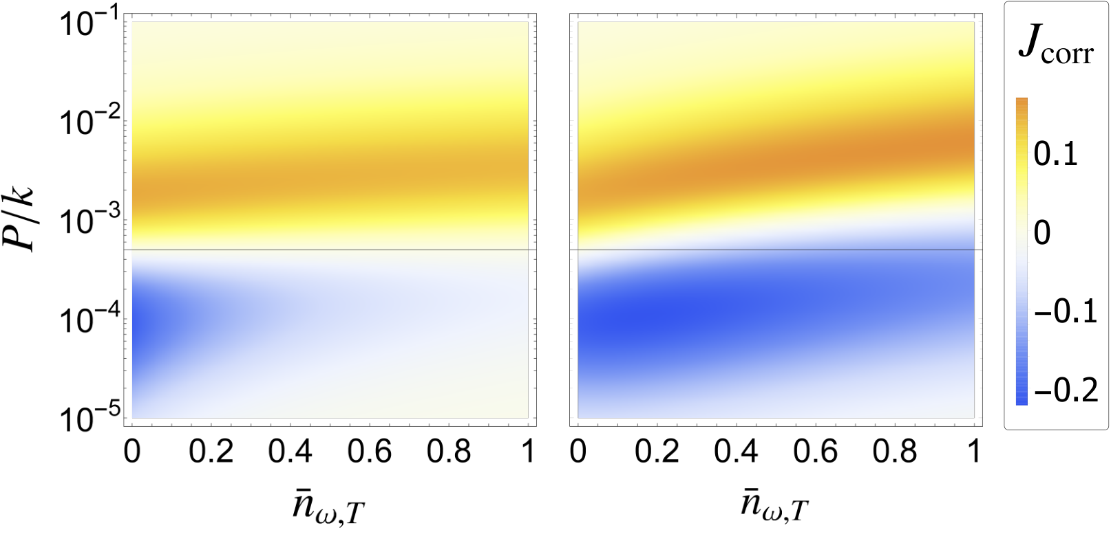
When , there is no difference between the 1ph and the 2ph models because . In contrast, the two models behave very differently for , as shown in Fig. 3 where we plot the steady value of in the two models as functions of the incoherent pumping and the baths temperature in the case of two TLSs, for and . A more varied dependence of the collective phenomena on temperature in the 2ph case is observed due to the increase of the collective dissipation rate with the temperature. In particular, remarkable differences are observed when is close to , since for this value of , in the 1ph case, for any , while this is not the case in the 2ph case. This can be also evinced by the analytical expression we have obtained for in the two-TLS case (see Appendix E.2) which shows that subradiance and superradiance are obtained when is, respectively, lower or higher than . This behavior of the sign of has been confirmed in all the other simulations that we have done (up to six TLSs). This means that for , since increases with temperature, subradiance is observed for any temperature different from zero in the 2ph case. One could wonder if part of these differences arises just because the TLSs in the 2ph model have frequency so that, for the same temperature, they interact with local baths by means of a lower average excitation number. To check the extent of this effect we have also looked at the same plot using the frequency for the TLSs and the HO for the 1ph case finding only a partial reduction of the differences between the two models. An example of this issue is treated for a specific example in Fig. 4.
A different behavior of collective phenomena is still present in the case of a larger number of TLSs, as exhibited in Fig. 4(a), where the plot of in the steady state as a function of the incoherent pumping for four TLSs at a fixed temperature () clearly shows relevant differences in the two models, especially for the subradiance. In particular, in the 2ph case, a higher peak of both super and subradiance can be reached, even when the frequency of the TLSs and of the HO in the 1ph case is set equal to . A more striking different behavior of the two models can be obtained by studying the dependence of the steady value of on for specific values of the pump, as shown in Fig. 4(b). For no subradiance nor superradiance is visible in the 1ph case, while in the 2ph case a strong subradiance may be observed. An even more interesting case is obtained for . In this case, the system displays superradiance at in both models while it follows very different paths, depending on the model, when the temperature increases. In the 1ph model, is always positive and tends to zero for increasing temperature whereas, in the 2ph model, there is a temperature such that for . Therefore, in the 2ph model, the system can go into a subradiant zone inaccessible through the 1ph interaction at fixed pumping.
VI Conclusions
In summary, we have studied the case of a damped HO interacting with TLSs via a two-photon coupling in the bad-cavity limit in the presence of finite temperature baths, a coherent pumping on the HO, and an incoherent pumping on the TLSs, comparing it to the one-photon-coupling case. We have succeeded in applying a recent adiabatic elimination technique in the two-photon model to derive a master equation governing the collective evolution of the TLSs. This presents two fundamental differences compared to the dipolar case: an enhancement of the spontaneouslike emission rate, including a thermal contribution and a quadratic term in the coherent driving, and an increased temperature of the effective bath experienced by the TLSs. This unexpected phenomenology makes it possible to accelerate the generation of nondiagonal one-TLS steady states and to observe a drastic change of the temperature-dependent behavior of quantum collective phenomena, leading to a stronger resilience of these phenomena to high temperatures. We finally remark that the models here investigated can be feasibly implemented with both solid-state and atomic existing quantum technologies, as also discussed in Appendix A for the 2ph model in the solid-state context.
Acknowledgements.
N.P. acknowledges the financial support of the Observatoire des Sciences de l’Univers THETA Franche-Comté / Bourgogne for his research visit at the Université Paris Diderot (now Université de Paris). B.B. acknowledges support by the French “Investissements d’Avenir” program, project ISITE-BFC (Contract No. ANR-15-IDEX-03). N.P. and B.B. thank Andrea Smirne for useful discussions about the results of this Letter.Appendix A Circuit model

In this section, we provide a detailed description of a superconducting quantum circuit scheme that can implement the two-photon (2ph) Jaynes-Cumming Hamiltonian used in Eq. (1) of the main text for . Indeed, in the framework of circuit QED Blais et al. 2021 it is possible to engineer artificial atoms that are nonlinearly coupled with a single-mode quantum resonator Felicetti et al. 2018a; Felicetti et al. 2018b. We follow the derivation proposed in Ref. Felicetti et al. 2018b for the case of one qubit, generalizing it to the multiqubit case. Our scheme is depicted in Fig. 5 and it consists of an arbitrary number of flux qubits Orlando et al. 1999; van der Wal et al. 2000 coupled to a single superconducting quantum interference device (SQUID) resonator. For each qubit the coupling is realized via an inductance and the values of the coupling inductances are assumed to be the same for all the qubits. The SQUID is used in the linear regime so that, for the considered energy scales, it supports a quantum harmonic resonator mode. However, as shown in the following, the intrinsic nonlinearity of the device can lead to a dynamics governed by a two-photon coupling between the artificial atoms and the resonator. We will first derive an effective Lagrangian model of the circuit, and we will then quantize the corresponding Hamiltonian.
A.1 Lagrangian
Our starting point is the Lagrangian of the system Blais et al. 2021,
| (7) |
where the index runs over the flux qubits and where the different contributions of the SQUID, the flux qubits (FQ), and the coupling inductances (L) are given by
| (8) |
| (9) | ||||
| (10) |
Here, denotes the Josephson energy and the capacitance of the Josephson junctions (JJ) and composing the SQUID, which are assumed to be identical. As for the flux qubits, and are the Josephson energy and capacitance of the JJs labeled by and , while is a parameter, smaller than one, used to quantify the corresponding values and for the second JJ. The coupling inductances between each flux qubit and the SQUID are also assumed to be identical with value . Finally, all the variables denoted with a are the generalized fluxes associated to each element of the circuit Blais et al. 2021, and we have defined the reduced magnetic flux quantum as , where is the electron charge.
We now define symmetric and anti-symmetric SQUID variables as and and apply the flux-quantization rule Tinkham 2004; Blais et al. 2021 to the SQUID loop, obtaining , where is the external magnetic flux flowing through the SQUID loop. We can then rewrite the anti-symmetric variable in terms of the phases of the coupling inductances obtaining . We consider a constant external flux implying . Straightforward calculations allow us to rewrite the SQUID Lagrangian as,
| (11) |
where we have defined . Now, we turn our focus on the circuit elements composing the flux qubits, and we define and . We denote with the external flux on each qubit, which is taken to be the same for all flux qubits, and which is defined in the opposite direction with respect to . The flux-quantization rule for the qubit loop, , allows us to eliminate the phase variable of the second junction of each qubit: . We take also the external flux biasing the flux qubit to be constant implying , so we can write
| (12) |
We now take a perturbative approach based on the assumption that the coupling inductances are chosen to be so small that the following approximations are justified. In particular, we perform two main approximations: (1) we linearize the Lagrangian with respect to the coupling-inductance phase variables divided by , that is we expand to first order in , and then (2) we perform an adiabatic elimination of the corresponding degrees of freedom. Notice that this adiabatic elimination concerns only the detail of the circuit design and it is not related with the adiabatic elimination performed on the quantum model considered in the main text. To simplify the notation, let us define the gauge-invariant phase variables , where denotes generically the flux variable of any circuit element. We also define the frustration parameters and .
(1) First, we assume that the flux variables are small with respect to the reduced magnetic flux quantum, so that Eq.(A.1) and Eq.(A.1) can be linearized with respect to the variables . Thus, from Eq. (A.1) we obtain
| (13) |
Then, by linearizing Eq.(A.1) with respect to each we obtain,
| (14) |
where denotes the standard Lagrangian of the -th flux qubit van der Wal et al. 2000; Orlando et al. 1999,
| (15) |
(2) Now, we perform the adiabatic elimination on the degrees of freedom of the coupling inductances. These inductances appear in the following terms of the total Lagrangian [see Eqs. (10), (13), and (A.1)]:
| (16) |
The first line corresponds to interacting harmonic oscillators. Given the high symmetry of the coefficients, it is easy to find the normal frequencies Landau and Lifshitz 1976, which are given by
| (17) |
where the frequency has degeneracy . Here, is assumed to be so small that the frequency (which is clearly smaller than ) is much larger than the relevant characteristic frequencies of the other elements of the circuit. Moreover, the interaction of the inductances with the other elements of the circuit is such that, if is small enough, we can adiabatically eliminate the variables corresponding to the inductances by setting .
To simplify the notation let us define the following parameters:
| (18) |
Imposing in the Euler-Lagrange equation
| (19) |
we obtain the dependence of on the remaining dynamic variables,
| (20) |
where . Therefore,
| (21) |
where is the total number of flux qubits.
A.2 Hamiltonian
The system Hamiltonian can be derived implementing the Legendre transformation, i.e.,
| (25) |
where we use the standard definition of conjugate variables
| (26) |
We replace now the classical variables with quantum operators and we start using the hat formalism to avoid confusion. The total Hamiltonian can be written as
| (27) |
The SQUID Hamiltonian is given by
| (28) |
The Hamiltonian is given by the standard flux-qubit Hamiltonian , plus a correction proportional to the small parameter [since ]:
| (29) |
where
| (30) |
It is well known that the standard flux-qubit Hamiltonian has a strongly nonlinear eigenspectrum Orlando et al. 1999; van der Wal et al. 2000. As a result, for the relevant energy scale, the system dynamics is constrained in the lowest two-level subspace Orlando et al. 1999; van der Wal et al. 2000. In the next subsection we discuss the role of the additional term , and we show that it does not induce state leakage outside the low-energy subspace so that each flux qubit can indeed be considered as a two-level system (TLS). In the following, the two states of the low-energy subspace for the -th TLS are denoted as and and the Hamiltonian of each TLS is , where is the common transition frequency of the TLSs and is the usual -Pauli operator.
The last term in Eq. (27) corresponds to the nondipolar coupling Hamiltonian
| (31) |
We show in the following that, in a broad regime of parameters, such nondipolar coupling can be reduced to a two-photon interaction plus an additional correction to the flux-qubit Hamiltonian.
A.3 Effective model
We now assume that the phase of the SQUID junctions is small compared to the reduced magnetic flux quantum: . This is a standard approximation Blais et al. 2021 which is valid when the SQUID operates in the linear regime, that is in the limit of large Josephson energy for the two Josephson junctions, and , of the SQUID. Expanding up to second order the cosines and discarding constant terms in Eq. (28) we obtain,
| (32) |
Similarly, we obtain from Eq. (31)
| (33) |
where the first term is a free energy term of the qubit, while the second term is the origin of the nondipolar coupling.
We now introduce the standard ladder operators and of the quantum harmonic oscillator corresponding to the SQUID Hamiltonian of Eq. (32) in
| (34) |
where we have defined
| (35) |
where we have introduced the charging energy [we recall that ]. Equation (32) can be then rewritten as
| (36) |
where we have used and we have again disregarded constant terms.
Now, we redefine the total free Hamiltonian of a flux qubit as the sum of Eq. (29) and of the -th element of the first term in Eq. (33),
| (37) |
which corresponds to the standard Hamiltonian of a flux qubit plus two corrections. In the first two energy levels subspace we can write Orlando et al. 1999; van der Wal et al. 2000 , where is the usual -Pauli operator and the transition amplitude is the same for all the qubits because we have set a homogeneous and the operator has the same form for all qubits. Notice that the first correction, proportional to , corresponds to a constant energy offset, since in the two-level subspace, being the identity operator in a two-dimensional Hilbert space, and can be then disregarded. The second one, proportional to , can be compensated by a small adjustment of the frustration parameter leading to a renormalization of the qubit-cavity coupling van der Wal et al. 2000; Orlando et al. 1999. Therefore, these additional terms do not modify the behavior of the flux qubit, and so the latter can be faithfully modelized as a TLS. In this limit, the Hamiltonian of a flux qubit is then redefined as
| (38) |
Finally, we redefine the interaction Hamiltonian as given by only the second term in Eq. (33), which corresponds to the nondipolar interaction Hamiltonian between the TLSs and the resonator mode,
| (39) |
where we have defined the two-photon coupling strength as
| (40) |
Now, we consider the resonant case by setting and we redefine for this case the total system Hamiltonian up to second order in as the sum of Eqs. (36), (38), and (39), obtaining
| (41) |
where , , and , as in the main text, being and the usual raising and lowering operators for a TLS. Notice that, as shown in Ref. Felicetti et al. 2018b, the fourth-order corrections here neglected have a negligible impact on the system dynamics and spectral features.
Going to the interaction picture through the unitary operator , where , the interaction Hamiltonian becomes , with
| (42) |
For the regime of the parameters we explore in the main text (where ), the ubiquitous rotating-wave approximation (RWA) can be applied to Eq. (41) and (42), neglecting all the terms oscillating in the interaction picture. We can thus redefine the total Hamiltonian as the two-photon Jaynes-Cumming Hamiltonian used in Eq. (1) of the main text for (we remark that in the main text and in the following sections of the supplemental material the operators are not anymore marked by the “hat”):
| (43) |
An analysis of the RWA in an analogous context can be found in Felicetti et al. 2015.
| Qubit parameters | |||
|---|---|---|---|
| GHz | GHz | ||
| Resonator and inductances parameters | |||
| GHz | GHz | GHz | |
| Resulting parameters | |||
| GHz | GHz | GHz | |
To conclude this section, let us provide an example of a set of physical parameters that matches the required regime. We consider a system composed of 4 TLSs, as in the case of Fig. 4 of the main text. Notice that all model parameters can be analytically derived, except for the flux-qubit frequency which has been taken by an example of Ref. Orlando et al. 1999, where the same values for the flux-qubit circuit parameters have been used. The values of the various parameters are summarized in Table 1, which has been constructed as follows. First, we have taken the flux-qubit circuit parameters from Ref. Orlando et al. 1999, where the resulting frequency of the flux qubit is also given: GHz. Then, we have searched for a configuration of the resonator and inductances parameters (, , , and ) leading to GHz for the harmonic oscillator, well within the working range of circuit QED devices Blais et al. 2021. For the number appearing in the expression for of Eq. (40), we have used the value , which has been calculated for similar circuit parameters in the code used for Ref. Felicetti et al. 2018b. Regarding the inductances, from Eq. (20) one can estimate by excess the expectation value of the operator associated to the variable finding in modulus , which is consistent with the linearization procedure we have performed with respect to the variables . Morevoer, this choice of the circuit parameters leads to a value of the lowest inductances characteristic frequency well above the relevant energy scale, being more than 20 times larger than the flux qubits frequency 11 1 For convenience of the reader, we report in this note the formulas for the inductances normal frequencies in terms of the energetic circuit parameters: These formulas are equivalent to those of Eq. (17).. It follows that the adiabatic elimination we have made concerning the variables , , is well justified. Finally, we have , that is (this is the value considered in all the figures of the main text) if we take , where is the dissipation rate of the harmonic oscillator due to the interaction with its environment.
Concerning the flux qubits, the parameters are taken from Ref. Orlando et al. 1999 on the basis of the standard flux qubit Hamiltonian , i.e., the Hamiltonian of Eq. (37) without the two additional terms. It follows that the parameter values should be slightly calibrated in a real experimental realization in order to obtain the resonance . However, the engineering of flux qubit is a well-developed area of research and their effective frequency can be finely tuned in various ways, also adding additional elements to the circuit Blais et al. 2021. Even if the values of Table 1 do not exactly match those that would be used for our circuit, they are then a good indicator of the experimental values that would be in fact necessary.
We stress out that the values used in Table 1 are commonly implemented in nowadays experiments Blais et al. 2021 and that the proposed circuit design does not require any further improvement over standard circuit-QED technology.
Appendix B Adiabatic elimination technique
Here, we briefly resume the recently developed adiabatic elimination technique Azouit et al. 2017; Azouit 2017 that we have exploited in our analysis. To apply this technique we have to divide the system under study into two subsystems, one governed by a fast dynamics and the other one by a slow one. We call “system ” the fast system and “system ” the slow one. Moreover, the two subsystems have to interact weakly. As final requirement, system has to converge to a unique steady state, which we call , when it is influenced uniquely by its own Lindbladian. For a far more detailed discussion see Ref. Azouit 2017.
Following the prescription of Ref. Azouit 2017, the Lindbladian describing the evolution of the density matrix of the global system, , is given by
| (44) |
where is the quantity which will play the role of perturbative parameter in the expansion of system dynamics and each Lindbladian is of the form
| (45) |
where , , and
| (46) |
The interaction Hamiltonian can be written in the general form , where and are not necessarily hermitian and is a constant with the dimension of a frequency.
The goal of the adiabatic elimination procedure is to find the superoperator describing the dynamics of the reduced density matrix of system , , as
| (47) |
and to be able to return back to the global dynamics through
| (48) |
where, at any order in , is a Lindbladian and is a Kraus map. In our case, we want to obtain a second order equation for the dynamics of system since, at first order, the adiabatic elimination does not give rise to dissipative terms.
Due to the peculiarities of the method employed, the zero-order terms can be chosen with a certain arbitrariness. Following Ref. Azouit 2017, the simplest choice is and . Then, the first order reduced dynamics is given by Azouit 2017
| (49) |
where
| (50) |
The superoperator can be obtained as follows Azouit 2017:
| (51) |
where , h.c. indicates the hermitian conjugate, and and are defined in the following. In general, the superoperator has the form
| (52) |
where such that and . Notice that even if it could seem that the results of the procedure depend on the choice of the parameter , for the case we are going to examine the value of this parameter will be irrelevant.
In order to find the second order dynamics of system , it is useful to define two matrices whose elements are given by
| (53) |
The matrix is Hermitian and positive semi-definite. Then, there exists a non-unique matrix such that .
Appendix C Adiabatic elimination of the harmonic oscillator
Here, we apply the general method described in the previous section to the one-photon (1ph) and the 2ph models considered in the main text. There, system consists of an harmonic oscillator (HO) while system is an ensemble of TLSs. In particular, the starting point for this application is the Eq. (2) of the main text which describes the global dynamics of the two models and is given in the interaction picture. In the Schrödinger picture, the two models are described by the equation
| (56) |
where is the global density matrix in the Schrödinger picture, for the 1ph case and for the 2ph one, is given in Eq. (1) of the main text, and
| (57) |
The passage from the Schrödinger picture to the interaction one is, indeed, necessary to apply the adiabatic elimination method since the bare dynamics of both the TLSs and the harmonic oscillator is much faster than all other dynamics so that to separate the system into a fast and a slow part is not possible. Moreover, neglecting the interaction between the two subsystems, a steady state of the HO does not exist because of the time dependent part in the Hamiltonian describing the action of the coherent driving. The unitary operator used to move from the Schrödinger picture to the interaction one [i.e., from Eq. (56) to Eq. (2) of the main text, being ] is
| (58) |
where
| (59) |
In this section, we denote the reduced density matrix of the HO with in order to maintain the notation of the preceding section, while we call the reduced density matrix of the TLSs , without suffixes, in order to have the same notation of the main text.
As explained in the preceding section, we first need to obtain the steady state of the HO when it does not interact with the TLSs. This steady state is equal to Azouit 2017
| (60) |
where , , and
| (61) |
In other words, is a thermal coherent state obtained by applying to the thermal state with average energy the displacement operator corresponding to the coherent state in which the HO would be at zero temperature.
We choose to use as perturbative parameter the quantity so that . With this choice, we can write
| (62) |
where . Moreover, . Therefore, at first order in we get [see Eq. (50) with , , , and ]
| (63) |
since [using ]
| (64) |
To obtain the second order dynamics we need the superoperators . In this case, there are only two of them:
| (65) |
In order to calculate the matrix elements and of Eq. (B) we just need to compute terms like so that finding the explicit form of the operators is not necessary. Since , one can, for example, write
| (66) |
where is the adjoint Lindblad operator Breuer and Petruccione 2007; Azouit 2017. In the same way, one obtains the following quantities
| (67) |
The above formulas (and the resulting master equation) are valid for any but, from now on, we will deal explicitly with the cases because otherwise calculations become needlessly cumbersome. The result obtained in the case is already known in literature Azouit 2017. Nevertheless, we think that reporting here its derivation with this method can be helpful.
C.1 The 1ph case
For it is possible to write , with and . The adjoint master equation for the operator reads Azouit 2017; Breuer and Petruccione 2007
| (68) |
whose solution, and , implies
| (69) |
We recall that , where is a constant. Analogously, we can write and solve the associated differential equations. The solutions are equal to the ones for and with the substitution . It follows that
| (70) |
Now, we can calculate the elements of the and matrices. Using Eqs. (69) and (70) in Eq. (C), we obtain for (hereafter )
| (71) |
By inserting Eq. (C.1) in Eq. (B), we then have
| (72) |
We can set thus obtaining in Eq. (B):
| (73) |
Eventually, using Eqs. (54) and (63), we obtain as equation for the second order dynamics of the TLSs
| (74) |
where .
C.2 The 2ph case
The derivation of the reduced dynamics for proceeds analogously to the case, but it is more involved. We can write , with and . The adjoint master equation for the operator reads
| (75) |
whose solution, , , and , implies
| (76) |
Analogously, we can write and solve the associated differential equations. The solutions are equal to the ones for , , and with the substitution :
| (77) |
Now, we can calculate the elements of the and matrices. After straightforward but lengthy calculations, using Eqs. (76) and (C.2) in Eq. (C) and the following equalities
| (78) |
we obtain, for ,
| (79) |
Then, the and matrices are easily obtained by inserting Eq. (C.2) in Eq. (B):
| (80) |
Eventually, using Eq. (54) and setting as in the 1ph case, the second order dynamics of the TLSs reads
| (81) |
The above equation can be rewritten by operating the following substitutions
| (82) |
where
| (83) |
In this way, the 2ph model reduced master equation becomes
| (84) |
Notice that the quantity can also be written as
| (85) |
which is another way to display what is shown in Eq. (6) of the main text, i.e., the fact that the effective temperature of the collective bath as seen by the TLSs is higher than the actual temperature due to the action of the external coherent field on the harmonic oscillator.
C.3 Validity of the adiabatic elimination
We finally comment on the validity of the adiabatic elimination approximation which, in our setting, relies on the much higher rate of losses of the HO compared to its exchanges with the TLSs and requires stronger conditions than just . For example, for the 1ph coupling with one TLS, if the HO is in a Fock state with excitations and the TLS is in the ground state, the “Rabi oscillations” have angular frequency , leading to the condition . In the 2ph case, the same reasoning leads to . In our dynamics, at order zero [see Eqs. (60) and (61)] the HO is in a thermal coherent state with an average number of excitations . Then, we can roughly estimate the validity of the adiabatic elimination by using this value for in the above conditions. In general, we expect the approximation to not work properly also when since in this case the TLSs emission would compete with the HO losses.
Appendix D Mathematical mapping of the two models
The comparison of Eq. (C.1) and Eq. (C.2) shows that the master equation describing the dynamics of the TLSs can be cast in the same form for both models. For this reason, a mathematical mapping between the two models is obtainable. In particular, given the physical parameters in the 2ph model
| (86) |
contained in the effective parameters , the dynamics to which they give rise can be obtained in the 1ph model by different proper choices of the physical parameters. Denoting with an apex the effective quantities for this “simulation” in the 1ph model we get
| (87) |
We remark, however, that this mapping between the two models is a mathematical mapping and that there are situations in which the dynamics obtained in one model is not obtainable in the other one. For example, when the incoherent pumping is absent in the 2ph model, since [see Eq. (85)], in the 1ph model we could need to simulate the 2ph model, and this does not correspond to the case of an incoherent pumping term. Indeed, the physical reason for this incompatibility is the temperature-modifying effect of the coherent driving taking place only in the 2ph model [see Eq. (6) of the main text].
Appendix E Steady states
In this section, we report some details regarding the steady states of the TLS dynamics in the one- and two- TLS cases.
E.1 One-TLS case
In the case when system consists of just one TLS, it is described by the master equation
| (88) |
where and . The density matrix elements of the steady state are found to be
| (89) |
being for any , and .
An interesting limit case is obtained when is high enough that every term not containing it can be safely neglected. In the 1ph case, the result of this operation is
| (90) |
In the 2ph case, in this limit we have and so that
| (91) |
where we have used the notation . The case represented in Fig. 2 of the main text is the zero-temperature one, for which the above formulas become
| (92) |
In this case, the maximum of is obtained for . However, for this value of we are not anymore in the bad-cavity limit.
E.2 Two-TLS case
The steady state of two TLSs can be found analytically (we have done it using MATHEMATICA) but its form is very cumbersome and, therefore, we do not report it here. Here, we report the analytical form of in the case , analyzed in the maintext:
| (93) |
where . The sign of in Eq. (93) depends only on , which is temperature dependent only in the 2ph case. Our numerical simulations of the effective model indicate that this is true for any number of TLSs. We have checked this up to six of them.
References
- Haroche and Raimond (2006) S. Haroche and J.-M. Raimond, Exploring The Quantum: Atoms, Cavities, and Photons (Oxford University Press, 2006).
- Kirton et al. (2019) P. Kirton, M. M. Roses, J. Keeling, and E. G. Dalla Torre, Introduction to the Dicke Model: From Equilibrium to Nonequilibrium, and vice versa, Adv. Quantum Technol. 2, 1800043 (2019).
- Benedict (1996) M. G. Benedict, Super-Radiance: Multiatomic Coherent Emission (CRC, Boca Raton, FL, 1996).
- Gross and Haroche (1982) M. Gross and S. Haroche, Superradiance: An essay on the theory of collective spontaneous emission, Phys. Rep. 93, 301 (1982).
- Meiser et al. (2009) D. Meiser, J. Ye, D. R. Carlson, and M. J. Holland, Prospects for a Millihertz-Linewidth Laser, Phys. Rev. Lett. 102, 163601 (2009).
- Meiser and Holland (2010a) D. Meiser and M. J. Holland, Steady-state superradiance with alkaline-earth-metal atoms, Phys. Rev. A 81, 033847 (2010a).
- Meiser and Holland (2010b) D. Meiser and M. J. Holland, Intensity fluctuations in steady-state superradiance, Phys. Rev. A 81, 063827 (2010b).
- Auffèves et al. (2011) A. Auffèves, D. Gerace, S. Portolan, A. Drezet, and M. F. Santos, Few emitters in a cavity: From cooperative emission to individualization, New J. Phys. 13, 093020 (2011).
- Shammah et al. (2017) N. Shammah, N. Lambert, F. Nori, and S. De Liberato, Superradiance with local phase-breaking effects, Phys. Rev. A 96, 023863 (2017).
- Kirton and Keeling (2018) P. Kirton and J. Keeling, Superradiant and lasing states in driven-dissipative Dicke models, New J. Phys. 20, 015009 (2018).
- Shammah et al. (2018) N. Shammah, S. Ahmed, N. Lambert, S. De Liberato, and F. Nori, Open quantum systems with local and collective incoherent processes: Efficient numerical simulations using permutational invariance, Phys. Rev. A 98, 063815 (2018).
- Damanet et al. (2019) F. Damanet, A. J. Daley, and J. Keeling, Atom-only descriptions of the driven-dissipative Dicke model, Phys. Rev. A 99, 033845 (2019).
- Bonifacio et al. (1971a) R. Bonifacio, P. Schwendimann, and F. Haake, Quantum statistical theory of superradiance. I, Phys. Rev. A 4, 302 (1971a).
- Bonifacio et al. (1971b) R. Bonifacio, P. Schwendimann, and F. Haake, Quantum statistical theory of superradiance. II, Phys. Rev. A 4, 854 (1971b).
- Azouit et al. (2017) R. Azouit, F. Chittaro, A. Sarlette, and P. Rouchon, Towards generic adiabatic elimination for bipartite open quantum systems, Quantum Science and Technology 2, 044011 (2017).
- Azouit (2017) R. Azouit, Adiabatic elimination for open quantum systems, Theses, PSL Research University (2017).
- Leroux et al. (2010) I. D. Leroux, M. H. Schleier-Smith, and V. Vuletić, Implementation of Cavity Squeezing of a Collective Atomic Spin, Phys. Rev. Lett. 104, 073602 (2010).
- Tóth and Apellaniz (2014) G. Tóth and I. Apellaniz, Quantum metrology from a quantum information science perspective, J. Phys. A 47, 424006 (2014).
- Jahnke et al. (2016) F. Jahnke, C. Gies, M. Aßmann, M. Bayer, H. Leymann, A. Foerster, J. Wiersig, C. Schneider, M. Kamp, and S. Höfling, Giant photon bunching, superradiant pulse emission and excitation trapping in quantum-dot nanolasers, Nat. Commun. 7, 11540 (2016).
- Asenjo-Garcia et al. (2017) A. Asenjo-Garcia, M. Moreno-Cardoner, A. Albrecht, H. J. Kimble, and D. E. Chang, Exponential Improvement in Photon Storage Fidelities Using Subradiance and “Selective Radiance” in Atomic Arrays, Phys. Rev. X 7, 031024 (2017).
- Garcia-Vidal and Feist (2017) F. J. Garcia-Vidal and J. Feist, Long-distance operator for energy transfer, Science 357, 1357 (2017).
- Goban et al. (2015) A. Goban, C.-L. Hung, J. D. Hood, S.-P. Yu, J. A. Muniz, O. Painter, and H. J. Kimble, Superradiance for Atoms Trapped along a Photonic Crystal Waveguide, Phys. Rev. Lett. 115, 063601 (2015).
- DeVoe and Brewer (1996) R. G. DeVoe and R. G. Brewer, Observation of Superradiant and Subradiant Spontaneous Emission of Two Trapped Ions, Phys. Rev. Lett. 76, 2049 (1996).
- Jenkins et al. (2017) S. D. Jenkins, J. Ruostekoski, N. Papasimakis, S. Savo, and N. I. Zheludev, Many-Body Subradiant Excitations in Metamaterial Arrays: Experiment and Theory, Phys. Rev. Lett. 119, 053901 (2017).
- Pustovit and Shahbazyan (2009) V. N. Pustovit and T. V. Shahbazyan, Cooperative Emission of Light by an Ensemble of Dipoles Near a Metal Nanoparticle: The Plasmonic Dicke Effect, Phys. Rev. Lett. 102, 077401 (2009).
- Angerer et al. (2018) A. Angerer et al., Superradiant emission from colour centres in diamond, Nat. Phys. 14, 1168 (2018).
- Scheibner et al. (2007) M. Scheibner, T. Schmidt, L. Worschech, A. Forchel, G. Bacher, T. Passow, and D. Hommel, Superradiance of quantum dots, Nat. Phys. 3, 106 (2007).
- Mlynek et al. (2014) J. A. Mlynek, A. A. Abdumalikov, C. Eichler, and A. Wallraff, Observation of Dicke superradiance for two artificial atoms in a cavity with high decay rate, Nat. Commun. 5, 5186 (2014).
- Felicetti et al. (2018a) S. Felicetti, D. Z. Rossatto, E. Rico, E. Solano, and P. Forn-Díaz, Two-photon quantum Rabi model with superconducting circuits, Phys. Rev. A 97, 013851 (2018a).
- Felicetti et al. (2018b) S. Felicetti, M.-J. Hwang, and A. Le Boité, Ultrastrong-coupling regime of nondipolar light-matter interactions, Phys. Rev. A 98, 053859 (2018b).
- Felicetti et al. (2015) S. Felicetti, J. S. Pedernales, I. L. Egusquiza, G. Romero, L. Lamata, D. Braak, and E. Solano, Spectral collapse via two-phonon interactions in trapped ions, Phys. Rev. A 92, 033817 (2015).
- Cheng et al. (2018) X.-H. Cheng, I. Arrazola, J. S. Pedernales, L. Lamata, X. Chen, and E. Solano, Nonlinear quantum Rabi model in trapped ions, Phys. Rev. A 97, 023624 (2018).
- Puebla et al. (2019) R. Puebla, J. Casanova, O. Houhou, E. Solano, and M. Paternostro, Quantum simulation of multiphoton and nonlinear dissipative spin-boson models, Phys. Rev. A 99, 032303 (2019).
- Schneeweiss et al. (2018) P. Schneeweiss, A. Dareau, and C. Sayrin, Cold-atom-based implementation of the quantum Rabi model, Phys. Rev. A 98, 021801(R) (2018).
- Dareau et al. (2018) A. Dareau, Y. Meng, P. Schneeweiss, and A. Rauschenbeutel, Observation of Ultrastrong Spin-Motion Coupling for Cold Atoms in Optical Microtraps, Phys. Rev. Lett. 121, 253603 (2018).
- Goetz et al. (2018) J. Goetz, F. Deppe, K. G. Fedorov, P. Eder, M. Fischer, S. Pogorzalek, E. Xie, A. Marx, and R. Gross, Parity-Engineered Light-Matter Interaction, Phys. Rev. Lett. 121, 060503 (2018).
- Lv et al. (2018) D. Lv, S. An, Z. Liu, J.-N. Zhang, J. S. Pedernales, L. Lamata, E. Solano, and K. Kim, Quantum Simulation of the Quantum Rabi Model in a Trapped Ion, Phys. Rev. X 8, 021027 (2018).
- Minganti et al. (2016) F. Minganti, N. Bartolo, J. Lolli, W. Casteels, and C. Ciuti, Exact results for Schrödinger cats in driven-dissipative systems and their feedback control, Scientific reports 6, 26987 (2016).
- Malekakhlagh and Rodriguez (2019) M. Malekakhlagh and A. W. Rodriguez, Quantum Rabi Model with Two-Photon Relaxation, Phys. Rev. Lett. 122, 043601 (2019).
- Leghtas et al. (2015) Z. Leghtas et al., Confining the state of light to a quantum manifold by engineered two-photon loss, Science 347, 853 (2015).
- Travěnec (2012) I. Travěnec, Solvability of the two-photon Rabi Hamiltonian, Phys. Rev. A 85, 043805 (2012).
- Duan et al. (2016) L. Duan, Y.-F. Xie, D. Braak, and Q.-H. Chen, Two-photon Rabi model: Analytic solutions and spectral collapse, J. Phys. A 49, 464002 (2016).
- Maciejewski and Stachowiak (2017) A. J. Maciejewski and T. Stachowiak, A novel approach to the spectral problem in the two photon Rabi model, J. Phys. A 50, 244003 (2017).
- Xie et al. (2019) Y.-F. Xie, L. Duan, and Q.-H. Chen, Generalized quantum Rabi model with both one- and two-photon terms: A concise analytical study, Phys. Rev. A 99, 013809 (2019).
- Cong et al. (2019) L. Cong, X.-M. Sun, M. Liu, Z.-J. Ying, and H.-G. Luo, Polaron picture of the two-photon quantum Rabi model, Phys. Rev. A 99, 013815 (2019).
- Armenta Rico et al. (2020) R. J. Armenta Rico, F. H. Maldonado-Villamizar, and B. M. Rodriguez-Lara, Spectral collapse in the two-photon quantum Rabi model, Phys. Rev. A 101, 063825 (2020).
- Zou et al. (2020) F. Zou, X.-Y. Zhang, X.-W. Xu, J.-F. Huang, and J.-Q. Liao, Multiphoton blockade in the two-photon Jaynes-Cummings model, Phys. Rev. A 102, 053710 (2020).
- Garbe et al. (2017) L. Garbe, I. L. Egusquiza, E. Solano, C. Ciuti, T. Coudreau, P. Milman, and S. Felicetti, Superradiant phase transition in the ultrastrong-coupling regime of the two-photon Dicke model, Phys. Rev. A 95, 053854 (2017).
- Chen and Zhang (2018) X.-Y. Chen and Y.-Y. Zhang, Finite-size scaling analysis in the two-photon Dicke model, Phys. Rev. A 97, 053821 (2018).
- Cui et al. (2019) S. Cui, F. Hébert, B. Grémaud, V. G. Rousseau, W. Guo, and G. G. Batrouni, Two-photon Rabi-Hubbard and Jaynes-Cummings-Hubbard models: Photon-pair superradiance, Mott insulator, and normal phases, Phys. Rev. A 100, 033608 (2019).
- Garbe et al. (2019) L. Garbe, P. Wade, F. Minganti, N. Shammah, S. Felicetti, and F. Nori, Dissipation-induced bistability in the two-photon Dicke model, arXiv:1911.11694 (2019).
- Cui et al. (2020) S. Cui, B. Grémaud, W. Guo, and G. G. Batrouni, Nonlinear two-photon Rabi-Hubbard model: Superradiance, photon, and photon-pair Bose-Einstein condensates, arXiv:2006.09412 (2020).
- Villas-Boas and Rossatto (2019) C. J. Villas-Boas and D. Z. Rossatto, Multiphoton Jaynes-Cummings Model: Arbitrary Rotations in Fock Space and Quantum Filters, Phys. Rev. Lett. 122, 123604 (2019).
- Casanova et al. (2018) J. Casanova, R. Puebla, H. Moya-Cessa, and M. B. Plenio, Connecting nth order generalised quantum Rabi models: Emergence of nonlinear spin-boson coupling via spin rotations, Npj Quantum Inf. 4, 47 (2018).
- González-Gutiérrez and Torres (2019) C. A. González-Gutiérrez and J. M. Torres, Atomic Bell measurement via two-photon interactions, Phys. Rev. A 99, 023854 (2019).
- Loudon (2000) R. Loudon, The Quantum Theory of Light (OUP Oxford, 2000).
- Rumi and Perry (2010) M. Rumi and J. W. Perry, Two-photon absorption: An overview of measurements and principles, Adv. Opt. Photon. 2, 451 (2010).
- Rivera et al. (2016) N. Rivera, I. Kaminer, B. Zhen, J. D. Joannopoulos, and M. Soljačić, Shrinking light to allow forbidden transitions on the atomic scale, Science 353, 263 (2016).
- Flick et al. (2018) J. Flick, N. Rivera, and P. Narang, Strong light-matter coupling in quantum chemistry and quantum photonics, Nanophotonics 7, 1479 (2018).
- Blais et al. (2021) A. Blais, A. L. Grimsmo, S. M. Girvin, and A. Wallraff, Circuit quantum electrodynamics, Rev. Mod. Phys. 93, 025005 (2021).
- Breuer and Petruccione (2007) H.-P. Breuer and F. Petruccione, The Theory of Open Quantum Systems (Oxford University Press, New York, 2007).
- Rivas et al. (2010) Á. Rivas, A. D. K. Plato, S. F. Huelga, and M. B. Plenio, Markovian master equations: A critical study, New J. Phys. 12, 113032 (2010).
- Giorgi et al. (2020) G. L. Giorgi, A. Saharyan, S. Guérin, D. Sugny, and B. Bellomo, Microscopic and phenomenological models of driven systems in structured reservoirs, Phys. Rev. A 101, 012122 (2020).
- Streltsov et al. (2017) A. Streltsov, G. Adesso, and M. B. Plenio, Colloquium: Quantum coherence as a resource, Rev. Mod. Phys. 89, 041003 (2017).
- Wang et al. (2018) Z. Wang, W. Wu, G. Cui, and J. Wang, Coherence enhanced quantum metrology in a nonequilibrium optical molecule, New J. Phys. 20, 033034 (2018).
- Smirne et al. (2019) A. Smirne, A. Lemmer, M. B. Plenio, and S. F. Huelga, Improving the precision of frequency estimation via long-time coherences, Quantum Sci. Technol. 4, 025004 (2019).
- Orlando et al. (1999) T. P. Orlando, J. E. Mooij, L. Tian, C. H. van der Wal, L. S. Levitov, S. Lloyd, and J. J. Mazo, Superconducting persistent-current qubit, Phys. Rev. B 60, 15398 (1999).
- van der Wal et al. (2000) C. H. van der Wal, A. C. J. ter Haar, F. K. Wilhelm, R. N. Schouten, C. J. P. M. Harmans, T. P. Orlando, S. Lloyd, and J. E. Mooij, Quantum Superposition of Macroscopic Persistent-Current States, Science 290, 773 (2000).
- Tinkham (2004) M. Tinkham, Introduction to Superconductivity, 2nd ed. (Dover Publications, New York, 2004).
- Landau and Lifshitz (1976) L. D. Landau and E. M. Lifshitz, Course of Theoretical Physics, 3rd ed. (Butterworth-Heinemann, 1976), Vol. 1.
- (71)
For convenience of the reader, we report in this note the
formulas for the inductances normal frequencies in terms of the energetic
circuit parameters:
These formulas are equivalent to those of Eq. (17).