Satellite-to-Earth Quantum Key Distribution via Orbital Angular Momentum
Abstract
In this work, we explore the feasibility of performing satellite-to-Earth quantum key distribution (QKD) using the orbital angular momentum (OAM) of light. Due to the fragility of OAM states the conventional wisdom is that turbulence would render OAM-QKD non-viable in a satellite-to-Earth channel. However, based on detailed phase screen simulations of the anticipated atmospheric turbulence we find that OAM-QKD is viable in some system configurations, especially if quantum channel information is utilized in the processing of post-selected states. More specifically, using classically entangled light as a probe of the quantum channel, and reasonably-sized transmitter-receiver apertures, we find that non-zero QKD rates are achievable on sea-level ground stations. Without using classical light probes, OAM-QKD is relegated to high-altitude ground stations with large receiver apertures. Our work represents the first quantitative assessment of the performance of OAM-QKD from satellites, showing under what circumstances the much-touted higher dimensionality of OAM can be utilized in the context of secure communications.
I Introduction
As one of the most important applications in quantum communications, Quantum Key Distribution (QKD) has been proven to provide unconditional security Bennett and Brassard 1984. Recently, real-world implementations of satellite-based QKD (e.g. Liao et al. 2017; Yin et al. 2017) have pointed the way towards global-scale and highly-secure quantum communication networks Liao et al. 2018. The originally proposed QKD protocols (e.g. Bennett and Brassard 1984; Ekert 1991; Bruß 1998) mainly utilize 2-dimensional encoding. However, other QKD protocols have been generalized to the case of high-dimensional encoding (e.g. Bourennane et al. 2001), and their unconditional security has been proved (e.g. Bourennane et al. 2002; Cerf et al. 2002; Sheridan and Scarani 2010; Ferenczi and Lütkenhaus 2012). Quantum information can be encoded in any degree of freedom (DoF) of the photon, but most of the mainstream implementations of QKD (e.g. Yin et al. 2017; Liao et al. 2017; Liao et al. 2018) rely on polarization encoding - a typical 2-dimensional encoding scheme that limits the capacity of QKD systems due to an intrinsically bounded Hilbert space.
The Orbital Angular Momentum (OAM) of light has been considered as a promising DoF for quantum communications Vaziri et al. 2002. Unlike the polarization of light, the OAM of light can take arbitrary integer values Allen et al. 1992. The corresponding OAM eigenstates form an orthonormal basis that allows for quantum coding within a theoretically infinite-dimensional Hilbert space, opening up new possibilities for high-capacity quantum communications. As a key resource for quantum communications, entanglement can be encoded in OAM via the spontaneous parametric down-conversion (SPDC) process Mair et al. 2001; Dada et al. 2011. The distribution of OAM-encoded entanglement through the turbulent atmosphere has been intensively investigated in terrestrial free-space optical (FSO) channels (e.g. Leonhard et al. 2015; Hamadou Ibrahim et al. 2013; Roux et al. 2015; Ibrahim et al. 2014; Leonhard et al. 2018; Sorelli et al. 2019) with some demonstrating distribution over 3 km Krenn et al. 2015. A recent experiment suggests that OAM entanglement distribution could be feasible over an FSO channel of more than 100 km Krenn et al. 2016.
Besides the generation and distribution of OAM-encoded entanglement, other recent efforts have paved the way for the practical implementation of OAM-QKD. Any OAM superposition state can be efficiently encoded in single photons thanks to the versatility of a spatial light modulator (SLM) (see e.g. Bolduc et al. 2013; Mirhosseini et al. 2013a). The sorting of OAM-photons has also been made possible (e.g. Mirhosseini et al. 2013b; Larocque et al. 2017; Fickler et al. 2020), enabling the capability of performing multi-outcome measurements. Implementations of OAM-QKD have been demonstrated in laboratory conditions with 2-dimensional (e.g. Bouchard et al. 2018a) and higher-dimensional (e.g. Gröblacher et al. 2006; Mafu et al. 2013; Mirhosseini et al. 2015; Bouchard et al. 2018a) encoding. Efforts have also been made to investigate the practical feasibility of performing OAM-QKD in turbulent terrestrial FSO channels Ndagano and Forbes 2018; Goyal et al. 2016. Outside the laboratory, OAM-QKD has been demonstrated over turbulent FSO channels of 210 m Vallone et al. 2014, and 300 m Sit et al. 2017. Considering other types of medium, OAM-QKD has also been demonstrated over a 3 m underwater link Bouchard et al. 2018b and a 1.2 km optical fiber Cozzolino et al. 2019. However, most existing research on OAM-QKD has not considered the context of a satellite-based deployment. As such, the feasibility of long-range OAM-QKD via satellite is still not clear.
Previously we have studied the OAM detection performance in satellite-to-Earth communications Wang et al. 2019, and the feasibility of OAM-based entanglement distribution via satellite Wang et al. 2020. In this work, we explore the feasibility of satellite-to-Earth OAM-QKD. Our main finding is that, contrary to conventional wisdom, such QKD is indeed feasible. More specifically, we find that utilizing quantum channel information enables satellite-to-Earth OAM-QKD over a wide range of dimensions under all anticipated circumstances, including the circumstance where a sea-level ground station with a reasonably-sized receiver aperture is used. If channel information is not used, then feasible satellite-to-Earth OAM-QKD is confined to large telescopes situated at high-altitude observatories.
The remainder of this paper is as follows. In Section II we introduce the necessary background knowledge on OAM eigenstates, atmospheric propagation of light, and the generalized OAM-QKD protocol. In Section III we detail the system model for satellite-to-Earth OAM-QKD. In Section IV we present our key results on satellite-to-Earth OAM-QKD. In Section V we explore the use of quantum channel information to improve the practical feasibility of satellite-to-Earth OAM-QKD. Finally, concluding remarks are provided in Section VI.
II Background
II.1 OAM eigenstates
OAM-QKD protocols utilize OAM eigenstates and their superpositions for quantum encoding. In cylindrical coordinates, the general form of an OAM eigenstate is given by
| (1) |
where and are the radial and azimuthal coordinates, respectively, is the longitudinal distance, is the OAM quantum number, is the radial node number, and is the radial profile. OAM eigenstates with different values are mutually orthogonal. In this paper, we choose to be Laguerre-Gauss functions, making OAM eigenstates correspond to the Laguerre-Gaussian (LG) mode set Yao and Padgett 2011. is expressed in Eq. (2) as
| (2) | ||||
where , is the beam-waist radius, is the Rayleigh range, is the optical wavelength, is the optical wavenumber, and is the generalized Laguerre polynomial. We denote the single-photon OAM eigenstate of the mode as , and this notation is further simplified to as we only consider the subspace. We denote the set as the OAM basis and use it as the standard basis throughout this paper. Denoting the dimension as , the standard basis of -dimensional OAM-QKD contains mutually orthogonal OAM eigenstates and thus spans a -dimensional Hilbert space. Throughout this work we will denote such a -dimensional Hilbert space as the encoding subspace .
In this work, we consider a maximum OAM number of 4 to construct the encoding subspace . Specifically, we use the same approach adopted in Sorelli et al. 2019 to construct the encoding subspace . For , we consider a 2-dimensional encoding subspace spanned by a pair of OAM eigenstates with opposite OAM numbers (i.e. with ). For , we consider a 3-dimensional encoding subspace spanned by a pair of OAM eigenstates with opposite OAM numbers and the OAM eigenstate with zero OAM number (i.e. with ). For , more OAM numbers are involved. For example, for the 4-dimensional encoding subspace is spanned by two pairs of OAM eigenstates with opposite OAM numbers (i.e. with ).
II.2 Mutually unbiased bases
Denoted by , mutually unbiased bases (MUBs) are orthonormal bases defined on a -dimensional Hilbert space such that
| (3) |
where denotes the Kronecker delta function. MUBs play an important role in QKD since any system prepared in a state in one MUB gives outcomes with equal probability if measured in any other MUB. Therefore, if the eavesdropper measures the quantum signal in a wrong basis, she will acquire no information (in fact, she will introduce a disturbance).
It has been proven that, for a prime-power dimension there exists a complete set of MUBs Bandyopadhyay et al. 2002. In this work we consider a variety of dimensions ranging from to . When is a prime number (i.e. , , , in this work), a complete set of MUBs is found as eigenstates of different Weyl operators in the set . The operator is defined as
| (4) |
where denote the standard basis elements, and . The operator is defined as
| (5) |
When is a prime-power number but not a prime number (i.e. , , in this work), the construction of a complete set of MUBs becomes a harder task. In this work we adopt the sets of MUBs given in Klappenecker and Rötteler 2004; Spengler and Kraus 2013 for these dimensions. The only non-prime-power dimension considered in this work is . Since the maximum number of MUBs is not known for an arbitrary dimension, for we use only the 2 MUBs generated from the set (note that this has a negligible impact on the findings of this work). In OAM-QKD, the standard basis is the OAM basis, thus any is a superposition of OAM eigenstates that span the encoding subspace .
II.3 Optical propagation through turbulent atmosphere
The turbulent atmosphere is a random medium with random inhomogeneities (turbulent eddies) of different size scales that are upper-bounded and lower-bounded by an outer scale and an inner scale , respectively. These turbulent eddies give rise to small random refractive index fluctuations, causing continuous phase modulations on the optical beam. This leads to random refraction and diffraction effects, imposing distortions on the optical beam as it propagates through the atmospheric channel.
Under the paraxial approximation, the propagation of a monochromatic optical beam through the turbulent atmosphere is governed by the stochastic parabolic equation Andrews and Phillips 2005
| (6) |
where denotes the three-dimensional position vector (in Eq. (6) we use Cartesian coordinates for simplicity), is the transverse Laplacian operator, and represents the small refractive index fluctuation, with being the refractive index at . Note that the turbulent atmosphere satisfies and Andrews and Phillips 2005. In this work we numerically solve Eq. (6) using the split-step method Martin and Flatté 1988; Belmonte 2000; Schmidt 2010, which has been widely used to study atmospheric optical propagation under a variety of conditions. This method models the atmospheric channel using multiple slabs with a phase screen located in the midway of each slab. Two free-space (vacuum) propagations with one random phase modulation in between are repeatedly performed for each slab until the beam reaches the receiver plane Belmonte 2000. The split-step method has also been used to study the entanglement evolution of OAM-photon pairs in horizontal atmospheric channels, providing quantitative agreement with analytical results Ibrahim et al. 2014; Leonhard et al. 2018.
II.4 Generalized OAM-QKD protocol
QKD protocols can be described and implemented in both the prepare-and-measurement (P&M) paradigm and the entanglement-based (EB) paradigm. Although most implementations of QKD are based on the P&M scheme, all P&M QKD protocols have their EB equivalences (note that EB QKD has also been demonstrated over the satellite-to-Earth channel, see e.g. Yin et al. 2017). Furthermore, the EB paradigm is usually adopted to simplify the security analysis. Throughout this work we adopt the EB paradigm for OAM-QKD. Here we briefly recall the procedures of a -dimensional OAM-QKD protocol utilizing MUBs.
- 1.
Alice first generates entangled photon pairs. For every pair of the entangled photons Alice keeps one photon at her side and sends the other photon to Bob through a quantum channel.
- 2.
For every photon pair, Alice and Bob randomly (and independently) choose one of the MUBs and perform a -outcome measurement on their corresponding photon, giving each of them a -ary symbol.
- 3.
Alice and Bob start the sifting process where they reveal the MUBs that they used for their photon measurements. Specifically, they generate a sifted key by only keeping the symbols from the photon pairs jointly measured in the same MUB.
- 4.
In the parameter estimation process, Alice and Bob compare a small subset of their sifted data to estimate the average error rate .
- 5.
With the knowledge on , the two parties then carry out subsequent processes, including reconciliation (which mainly includes error correction) and privacy amplification, to produce a final secret key that Eve has no knowledge on.
III System Model
III.1 System settings
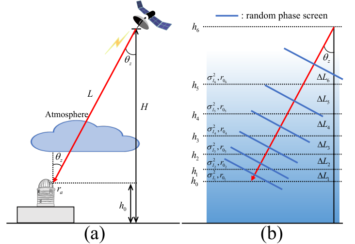
Throughout this work we denote the satellite and the ground station as Alice and Bob, respectively. In this section, we describe the system settings for satellite-to-Earth OAM-QKD (as illustrated in Fig. 1(a)). The ground-station altitude is denoted as , the satellite zenith angle at the ground station is denoted as , and the satellite altitude at is denoted as . The channel distance is given by . We denote the aperture radius at the ground station receiver as . To perform OAM-QKD, Alice is equipped with an on-board SPDC source that generates entangled OAM-photon pairs. Both Alice and Bob are equipped with versatile OAM mode sorters that can randomly switch between all available MUBs and perform the corresponding -outcome measurements.
The schematic diagram in Fig. 2 illustrates our deployment strategy for satellite-to-Earth OAM-QKD, in addition to all effects we consider. These include turbulence-induced crosstalk, loss (due to a finite-sized aperture), misalignment (due to imperfect beam tracking), and tomography noise (which leads to imperfect channel conjugation when classically entangled light is used as a probe to characterize the quantum channel).
Unless otherwise specified, the following assumptions are adopted throughout this work:
- 1.
We assume that Alice and Bob are perfectly time-synchronized, and they will discard any event where the photon sent by Alice does not click any of Bob’s detectors.
- 2.
We assume that the OAM mode sorters used for measurement have a separation efficiency of unity and introduce no additional loss.
- 3.
For any specific dimension , we only consider OAM-QKD protocols utilizing all MUBs. We restrict ourselves to the infinite key limit, therefore the sifting efficiency is set to 1. We also assume a reconciliation efficiency of 1.
- 4.
In the security analysis we assume that Eve controls the quantum channel and performs a collective attack.
III.2 Satellite-to-Earth atmospheric channel
III.2.1 Turbulence characterization
The strength of the optical turbulence within a satellite-based atmospheric channel can be described by the structure parameter as a function of altitude . can be described by the widely used Hufnagel-Valley (HV) model Andrews and Phillips 2005
| (7) | ||||
where is the ground-level (i.e. sea-level, ) turbulence strength in . In the above equation, is the root-mean-square wind speed in m/s which is given by
| (8) |
where is the altitude-dependent wind speed profile. In this paper we adopt the Bufton wind speed profile Andrews and Phillips 2005
| (9) |
where is the ground-level wind speed.
The effect of the atmospheric turbulence on a propagating beam is quantified by two parameters, namely the scintillation index and the Fried parameter . The scintillation index is the normalized variance of the intensity. For satellite-to-Earth channels under weak-to-strong turbulence, this parameter is given by Andrews and Phillips 2005
| (10) |
with being the Rytov variance,
| (11) |
The Fried parameter quantifies the coherence length of the turbulence-induced phase errors in the transverse plane. For satellite-to-Earth channels, this parameter is given by Andrews and Phillips 2005
| (12) |
III.2.2 Channel modeling
To perform the split-step method we divide the satellite-to-Earth atmospheric channel into slabs bounded by specific altitudes with ranging from 1 to (note that is the ground-station altitude, and a larger indicates a higher altitude). For the slab bounded by and , its thickness can be estimated as (note that ). In order to characterize the turbulence within each slab, both and are evaluated locally (for the turbulent volume of their corresponding slab). We denote the scintillation index and the Fried parameter for the slab as and , respectively. To accurately model the atmospheric channel using multiple slabs with a phase screen located in the midway of each slab, we meet the two conditions described in Martin and Flatté 1988 (i.e. and ) by setting and through a numerical search. A schematic illustration of our channel modeling (with ) is provided in Fig. 1(b). In our simulations ranges from to depending on specific settings.
After determining the widths of the atmospheric slabs, the realizations of the corresponding phase screens are generated using the Fast-Fourier-Transform (FFT)-based spectral domain algorithm McGlamery 1967. This method involves the filtering of a complex Gaussian random field using the phase power spectral density (PSD) function of the atmospheric turbulence. In this paper, we adopt the modified von Karman model, giving the phase PSD function for the slab
| (13) |
where is the magnitude of the two-dimensional spatial frequency vector in the transverse plane in cycles/m, , and Schmidt 2010.
For the free-space propagation, we utilize the FFT-based angular spectrum method (for details of this method one can refer to e.g. Goodman 1996; Schmidt 2010). In this study we utilize a physical optics propagation library named PROPER Krist 2007 to perform this method.
III.2.3 Quantum state evolution
To illustrate the undesirable decoherence effects caused by the atmospheric turbulence, we formally describe the evolution of an OAM eigenstate within a satellite-to-Earth channel. Assuming that Alice sends a single-photon OAM eigenstate to Bob’s ground station through an atmospheric channel. Under one realization of the atmospheric channel, the evolution of such a single-photon OAM eigenstate can be described by a unitary operator Sorelli et al. 2019. Denoting the received state as , we have
| (14) |
The received single-photon state can be expanded in the OAM basis as
| (15) |
where .
In this work, the evolution of a single-photon OAM eigenstate is simulated by the atmospheric propagation of the corresponding classical LG beam via the split-step method. In Fig. 3 we plot the intensity and phase profiles of an beam after vacuum propagation (i.e. propagation without atmospheric turbulence) and one realization of atmospheric propagation. After a vacuum propagation, we have due to the orthogonality of OAM eigenstates. After atmospheric propagation, however, the turbulence-induced distortions lead to crosstalk. At the receiver, is generally a superposition of OAM eigenstates, and thus it is no longer orthogonal to any OAM eigenstate. The resulting crosstalk causes entanglement decay and thus degrades the performance of OAM-QKD.

III.3 OAM-QKD over satellite-to-Earth channel
Now let us analyze the performance of OAM-QKD protocols introduced in Section II.4 over the satellite-to-Earth channel. Specifically, we are interested in the achievable QKD performance over the satellite-to-Earth channel. The QKD performance is quantified by the secret key rate in bits per sent photon, and throughout this work we use the unit bits per photon for short.
For a -dimensional OAM-QKD protocol, Alice generates OAM-photon pairs, each pair being in the maximally entangled state
| (16) |
where is a -dimensional encoding subspace. From each pair one photon is sent to Bob through a satellite-to-Earth quantum channel. At the output, the quantum state shared between Alice and Bob before any measurement is given by
| (17) |
where denotes an identity operator acting on Alice’s photon, and denotes an infinite-dimensional Hilbert space.
Although the initial state can be considered as a finite-dimensional state living in the subspace, due to the crosstalk it spreads over the entire infinite-dimensional Hilbert space. Since a practical system can only utilize a finite-dimensional encoding subspace, a necessary procedure is to project the output state onto the original subspace. This procedure is realized by a post-selection at Bob’s side, giving a post-selected (and un-normalized) state
| (18) |
where is the filtering operator acting on Bob’s photon. Since Bob has no information on , his filtering operator is equal to . By setting the post-selected state in Eq. (18) can be explicitly given as11 1 We will later show in Section V.1 that with channel information available Bob can adopt a different choice of , giving a different form of .
| (19) |
Note that is not normalized. In fact, the atmospheric propagation and the post-selection together form a completely positive (and non-trace-preserving) map . It is obvious that the post-selection results in a loss of photons. However, this operation will not give Eve any information, since the lost photons are simply discarded by Alice and Bob and will not be used in key generation.
Since we are not interested in any specific realization of the atmospheric channel, we perform an ensemble average of over different channel realizations. After averaging over channel realizations and performing re-normalization, the averaged state shared between Alice and Bob can be given as a mixed state described by
| (20) |
where denotes an ensemble average, and is the trace required for re-normalization. Note that quantifies the photon survival fraction after post-selection.
Now we briefly recall how security analysis is performed and how key rate is calculated for our OAM-QKD protocols (for a complete and rigorous security analysis, one can refer to Sheridan and Scarani 2010; Ferenczi and Lütkenhaus 2012). Utilizing the photons that survive the post-selection, the secret key rate can be expressed as22 2 Note, here the key rate is per photon actually used in the key generation. For every photon sent (transmitted) it can be ’lost’ either by being not hitting the receiver, or by not being post-selected via the projection operation. The parameter states the fraction of sent photons that survive both these loss events. Effectively, the finite-sized receiver aperture is absorbed into the post-selection process.
| (21) |
where is the classical mutual information between Alice and Bob, and is quantum information between Alice and Eve. Considering the fact that Eve holds a purification of , can be explicitly given as
| (22) |
where denotes the von Neumann entropy, denotes Alice’s measurement outcome, denotes the probability distribution of , and is the state of Bob’s photon conditioned on . In the security analysis it is assumed that all errors are caused by Eve’s eavesdropping attempts. The average error rate can be expressed as
| (23) |
Starting from Eq. (21), (22), is found to be a function of Sheridan and Scarani 2010; Ferenczi and Lütkenhaus 2012. For a -dimensional QKD protocol utilizing all MUBs, can be calculated as
| (24) | ||||
Recalling a non-unity photon survival fraction , the achievable secret key rate is given by
| (25) |
IV Numerical Evaluation of QKD Performance
In this section, we numerically evaluate the performance of the satellite-to-Earth OAM-QKD protocols analyzed in Section III.3. We carry out Monte Carlo simulations to numerically evaluate the secret key rate . First, we generate 4000 independent realizations of the satellite-to-Earth channel. For each channel realization we perform a series of atmospheric propagations using the split-step method to obtain a realization of (see Eq. (18)). Afterwards, realizations of are used to obtain and (see Eq. (20)). Then is evaluated from (see Eq. (23)), and is then evaluated from (see Eq. (24)). Finally, can be evaluated using and (see Eq. (25)).
IV.1 General settings
We restrict ourselves to the case of a low-Earth-orbit (LEO) satellite with a maximum satellite altitude . We consider two zenith angles, and , giving a maximum channel distance of and , respectively. Note that a higher leads to worse performance. This is because the beam radius on atmospheric entry increases with (due to diffraction), and this in turn results in increased distortion on the beam. A larger also leads to worse performance, since the photon travels a longer distance within the turbulent atmosphere. Unless otherwise stated, when we refer to our results we will mean for all considered values (i.e. from to ) and for all considered values (i.e. and ). Also, throughout this work QKD performances are compared at the same satellite altitudes under the same zenith angles.
For the atmospheric parameters, we set which accords with a realistic setting adopted in Guo et al. 2018. We set , giving a value of . We set m and cm for the atmospheric turbulence Andrews and Phillips 2005; Belmonte 2005. For the optical parameters, we set in accord with existing entanglement sources (e.g. Magnitskiy et al. 2015), and set to .
The loss of signal at the receiver will be a function of several system parameters as well as the atmospheric conditions. The beam width at the receiver is critical in determining the loss of signal, and is largely dependent on system parameters such as transmitter aperture (sets the beam waist ), and the distance between the satellite and the ground station. For a given optical wavelength, a given beam width at the receiver, and a given channel distance, the transmitter beam waist required can be easily determined. However, in our calculations we simply set the beam waist (in effect the transmitter aperture). To orientate ourselves, we note that the Micius satellite (which orbits at an altitude of about ), with an aperture size of m, provided a beam width of at ground level at a channel distance of Liao et al. 2017; Yin et al. 2017. For a satellite altitude of , the smallest beam width at ground level we will have in our calculations will be , corresponding to a loss at a receiver aperture of m radius (for a sea-level receiver, and a zenith angle of , this corresponds to our ).
We perform all simulations using a numerical grid of points with a spatial resolution33 3 Note, the spatial resolution (i.e. the grid spacing in the transverse plane) could be adaptively varied along the propagation path to minimize numerical errors in FFT-based wave propagation methods Schmidt 2010. However, in this work we fix the spatial resolution throughout the simulation. To validate this we perform a vacuum propagation over the length of the channel and compare the resulting simulated beam profile with an independently-derived analytical profile at the same channel distance. Such a test is performed for all considered channel distances and for LG beams with all considered OAM numbers, and we find that all numerical errors are negligible. We also note, when no phase modulation is set at the phase screens, our simulation results give . of . In generating the random phase screens using the FFT-based method, 3 orders of subharmonics are added using the method introduced in Lane et al. 1992 to accurately represent the low-spatial-frequency components contributed by large-scale turbulent eddies.
IV.2 Ideal circumstances
We first explore a rather ideal circumstance for the receiver. Adopting all settings of Section IV.1, we initially set the ground-station altitude to to avoid the strong atmospheric turbulence near the sea level. We also first adopt a large receiver aperture of , thus providing a zero-loss scenario.
First we investigate the performances of 2-dimensional and 3-dimensional OAM-QKD for different values under such an ideal circumstance. For 2-dimensional OAM-QKD, we find that a large value generally leads to a higher secret key rate. Under , positive key rates of 0.03, 0.05, 0.06 bits/photon can be achieved at for , respectively. Under , we observe a reduction in the secret key rate ranging from to . Specifically, only leads to a positive key rate of bits/photon at . For 3-dimensional OAM-QKD, we find that a larger value does not always lead to a higher secret key rate. Under , despite the observation that does not lead to any positive key rate, there is no significant correlation between the achievable secret key rate and for . Moreover, no positive key rate can be achieved at for any considered value. Under , we find that no positive key rate can be achieved by 3-dimensional OAM-QKD. By comparing the QKD performances, we find that the performance of 3-dimensional OAM-QKD is overall inferior to the performance of 2-dimensional OAM-QKD over the satellite-to-Earth channel for a given value.
We then compare the performances of OAM-QKD of dimensions ranging from 2 to 9 under , and find that the QKD performance decreases as the dimension increases44 4 When OAM-QKD of a dimension larger than 3 is involved in a performance comparison, for each dimension we choose a specific encoding subspace that maximizes the key rate.. Specifically, we find that no performance advantage can be achieved, by OAM-QKD of any dimension, against 2-dimensional OAM-QKD at . Furthermore, we find that OAM-QKD of dimensions larger than 5 achieve no positive key rate at all considered satellite altitudes and under all considered zenith angles. No positive key rate can be achieved by OAM-QKD of dimensions larger than 2 under .
It is widely anticipated that the use of higher-dimensional QKD can improve noise resistance and lead to a higher secret key rate. However, all the observations reported in this subsection clearly indicate that an increased dimension cannot improve the performance of OAM-QKD over the satellite-to-Earth channel, even under the ideal circumstance. This finding can be explained by the fact that the maximally OAM-entangled state of a higher dimension is less robust against turbulence (note that the similar phenomenon has been observed in e.g. Sorelli et al. 2019). This will lead to an increased error rate which can be large enough to nullify the advantage of higher-dimensional QKD. Therefore, a lower secret key rate is achieved in spite of a higher photon survival fraction (due to an enlarged encoding subspace). In other words, the theoretical capacity advantage provided by increasing the dimension in OAM-QKD is negated by the atmospheric turbulence over the satellite-to-Earth channel.
IV.3 Realistic circumstances
Now we extend our scope to more realistic circumstances. Specifically, we discuss the impact of loss, and a lower ground-station (receiver) altitude, on the feasibility of satellite-to-Earth OAM-QKD.
IV.3.1 Loss
The main source of loss in a satellite-to-Earth channel is diffraction loss. Diffraction loss is state-dependent in OAM-QKD since OAM eigenstates with different OAM numbers experience different amounts of diffraction Padgett et al. 2015. In order to investigate the impact of loss on the feasibility of satellite-to-Earth OAM-QKD, we adopt all settings of Section IV.2 except setting the radius of the receiver aperture to . At and under , setting gives losses of 1 dB, 3.4 dB, 6.9 dB, 11.3 dB, 16.7dB to OAM eigenstates with OAM numbers , , , , , respectively. We then re-evaluate the performances of 2-dimensional and higher-dimensional OAM-QKD.
In Fig. 4 we compare the performances of 2-dimensional OAM-QKD, achieved with and (zero loss), under and . From this figure, we see that the loss degrades the performance of 2-dimensional OAM-QKD, and such a performance degradation is more significant for a larger value.
Higher-dimensional OAM-QKD is more sensitive to loss. For 3-dimensional OAM-QKD, after setting we find that no positive key rate can be achieved at under . For OAM-QKD of dimensions larger than 3, setting we find that no positive key rate can be achieved at . Comparing the performances of OAM-QKD of different dimensions under loss, we find that 2-dimensional OAM-QKD is more robust against loss compared to higher-dimensional OAM-QKD. Indeed, the loss has a greater impact on higher-dimensional OAM-QKD due to its state-dependent nature (see related discussions in e.g. Zhao et al. 2019).
IV.3.2 Receiver altitude
Lowering the ground-station altitude increases the turbulence strength, and intuitively this can degrade QKD performance. To see whether satellite-to-Earth OAM-QKD is feasible under lower ground-station altitudes, we adopt all settings of Section IV.2 except for lower values. In Fig. 5 we compare the performances of 2-dimensional OAM-QKD, under , under different ground-station altitudes . From this figure, we clearly see that the use of a lower ground-station altitude degrades the performance of 2-dimensional OAM-QKD at a given satellite altitude. We see that a positive key rate can still be achieved for at under . Under we find that no positive key rate can be achieved at under .
OAM-QKD of a higher dimension is more sensitive to . For 3-dimensional OAM-QKD, we find that a larger value is not more robust against performance degradation. We also find that, for , no positive key rate can be achieved by 3-dimensional OAM-QKD at even under . For OAM-QKD of dimensions larger than 3, for we find that no positive key rate can be achieved at even under .
IV.3.3 Sea-level receiver with reasonably-sized aperture
Then we adopt all settings of Section IV.1 and jointly set and to reflect a more realistic scenario where a sea-level receiver with a reasonably-sized aperture is used. Unfortunately, we find that no positive key rate can be achieved by OAM-QKD of any dimension, even under .
V Feasibility Through Channel Information
In all previous sections we have assumed that channel knowledge is unavailable. It is intuitive to think that channel information can be used to improve QKD performance. Indeed, in quantum communications a natural paradigm is to characterize the quantum channel through quantum process tomography (QPT) Chuang and Nielsen 1997; Altepeter et al. 2003, and cancel out the turbulence-induced effects accordingly Ndagano et al. 2017. However, QPT is performed at the single-photon level, making the real-time characterization of quantum channels a challenging job. Recently it has been discovered that the state evolution of the classically entangled DoFs is equivalent to the state evolution of quantum entangled photons Ndagano et al. 2017. Such an equivalence allows for the use of non-separable (i.e. DoF-entangled) states of classical light to characterize the quantum channel (e.g. Ndagano et al. 2017; Ndagano and Forbes 2018; Mabena and Roux 2017; Mabena and Roux 2020). By performing a state tomography on the output classical light, the quantum channel can be readily characterized in real time (for a comprehensive tutorial, see e.g. Toninelli et al. 2019).
In this section we explore the use of quantum channel information to improve the practical feasibility of satellite-to-Earth OAM-QKD. Inspired by Ndagano et al. 2017; Ndagano and Forbes 2018, we utilize the quantum channel information acquired through a real-time quantum channel characterization utilizing non-separable states of classical light, and apply a quantum channel conjugation at the ground station. By quantum channel information we mean the Kraus operator of the channel, and by quantum channel conjugation we mean the application of a quantum conjugate filter that cancels out the turbulence-induced crosstalk.
V.1 General method
In this section, we demonstrate how a conjugate filter could be found, and we also analyze the impact of using that filter on OAM-QKD. The non-separable states of classical light we use for channel characterization is given in the general form Mabena and Roux 2017
| (26) |
where the first DoF is a DoF that is not affected by the turbulent atmosphere (e.g. polarization or wavelength), the second DoF denotes the OAM DoF of light, indicates different basis elements in these DoFs, and denotes the expansion coefficients such that . We denote the encoding subspaces of and as and , respectively. To faithfully characterize the quantum channel under study, it is required that and .
In an OAM-QKD protocol Alice prepares OAM-photon pairs in the maximally entangled state described by Eq. (16). To help characterize the quantum channel Alice also generates classical light in the corresponding non-separable state described by Eq. (26). While sending one photon of each entangled photon pair to Bob, Alice simultaneously sends the classical light through the same channel55 5 We assume that the classical light is made orthogonal to the quantum signal using polarization or wavelength multiplexing techniques. For example, if the polarization (wavelength) DoF is used to construct the non-separable state in Eq. (26), the wavelength (polarization) DoF should be used for multiplexing. We note that the turbulence effect on a propagating beam is wavelength-dependent, and this can potentially cause errors in quantum channel characterization. For simplicity, we assume that the wavelengths used for multiplexing and for constructing the non-separable state are chosen to be close enough to the wavelength of the quantum signal. Under such an assumption, the wavelength-dependent nature of the turbulence effect becomes negligible (see discussions in e.g. Mabena and Roux 2017).. Since the state evolution of is equivalent to the state evolution of , under a specific channel realization Bob can characterize the one-sided OAM quantum channel in the encoding subspace by performing a state tomography on the received classical light. Specifically, Bob finds the Kraus operator that satisfies
| (27) |
where denotes the state of the received classical light at Bob’s side. Note that the right-hand side of Eq. (27) is known to Bob via his state tomography.
The Kraus operator can be expressed in its polar decomposition as
| (28) |
where is a unitary operator and is a positive Hermitian operator. can be expressed in its spectral decomposition
| (29) |
where and denote the eigenvalues of and their corresponding eigenvectors, respectively. Note that can be expressed as superpositions of the standard basis elements.
Considering the fact that are smaller than 1, the conjugate filter cannot be directly constructed as . This is because has eigenvalues larger than 1 and thus cannot be physically implemented due to a violation of the no-cloning theorem66 6 One can show that, directly applying leads to a noiseless amplification. Such an operation is not allowed in a deterministic fashion by the no-cloning theorem.. To construct a conjugate filter that does not violate the no-cloning theorem, inspired by the idea in Ndagano and Forbes 2018 we consider a conjugate filter that achieves . Specifically, we construct the conjugate filter as
| (30) |
where . Note that in Eq. (30) is a local Procrustean filter which can be physically implemented (see experimental demonstrations of OAM Procrustean filters in e.g. Vaziri et al. 2003; Dada et al. 2011; Chen and Wu 2012).
Under every channel realization, Bob constructs the Kraus operator , constructs the conjugate filter , and applies on his photon. Therefore, Alice and Bob share a post-selected state of the form
| (31) |
Note that is not normalized. From Eq. (31) it can be seen that the quantum channel conjugation results in a probabilistic entanglement distillation. After averaging over channel realizations and performing re-normalization, is now given by
| (32) |
where is the photon survival fraction when the quantum channel conjugation is applied. Note that can be interpreted as the probability of success of the quantum channel conjugation (which can be as low as in extreme cases). Following the descriptions in Section III.3, and can be then used to evaluate the secret key rate . It can be inferred from Eq. (32) that is achieved by the quantum channel conjugation at the cost of a low photon survival fraction.
Here we summarize the assumptions made, regarding the quantum channel characterization and the quantum channel conjugation, in this section. For simplicity, we assume that the channel Kraus operator is constructed without error (i.e. perfect state tomography on classical light), and the exact conjugate filter is applied to Bob’s photon without error. Furthermore, these operations are assumed to be performed in real time. Such an assumption indicates that the time taken to perform a state tomography on the classical light is less than the coherence time of the atmospheric channel (typically on the order of milliseconds Andrews and Phillips 2005). Although no experiment has been demonstrated so far to indicate how fast such a state tomography can be done, in principle all the projective measurements required by such a state tomography can be done simultaneously with high signal-to-noise ratio. In addition, a recent work Zhu et al. 2019 has demonstrated that a complete state tomography can be done in one shot if the classical light is in a pure state (note that this is valid under every specific channel realization). We further notice that the paradigm adopted here resembles the concept of Adaptive Optics (AO) where a servo loop system tracks (with a wavefront sensor) and corrects (with a deformable mirror) the turbulence effect in a real-time fashion. Given the fact that current AO systems have no significant trouble keeping up with the temporal evolution of turbulence, we believe that the quantum channel characterization and the following quantum channel conjugation can also be performed in real time.
V.2 QKD performance with quantum channel conjugation
To numerically investigate the impact of the quantum channel conjugation on QKD performance, we adopt the settings of Sections IV.2, IV.3 and re-evaluate the performances of satellite-to-Earth OAM-QKD of different dimensions. In 2-dimensional OAM-QKD, we assume that the vector vortex beam is used for quantum channel characterization (for a detailed review on vector vortex beams one can refer to e.g. Rosales-Guzmán et al. 2018). Specifically, Eq. (26) is explicitly given by
| (33) |
where denote right and left circular polarization states, respectively. In 3-dimensional OAM-QKD, the vector vortex beam cannot be used due to the constraint of the 2-dimensional Hilbert space imposed by the polarization DoF. It has been proposed in Mabena and Roux 2017 that the wavelength DoF of light is a promising candidate to replace the polarization DoF of light in . Specifically, Eq. (26) is explicitly given by
| (34) |
where denote different wavelengths. Although no experiment has been demonstrated so far, the use of classical light in a state described by Eq. (34) is theoretically feasible Mabena and Roux 2017. Since there is no fundamental limitation on dimension if the wavelength DoF is adopted, we also use this paradigm for quantum channel characterization in OAM-QKD of higher () dimensions.
First, we compare the QKD performances achieved with and without the quantum channel conjugation under the ideal circumstances in Section IV.2. We find that, with the help of the quantum channel conjugation, positive (and improved) secret key rates can be achieved by OAM-QKD of all considered dimensions at all considered satellite altitudes under all considered zenith angles. We also find that the use of smaller OAM numbers leads to a higher secret key rate. For 2-dimensional and 3-dimensional OAM-QKD, this means a smaller value leads to better performance. For OAM-QKD of dimensions larger than 3 this means using OAM numbers as small as possible to construct the encoding subspace leads to a better performance. Comparing the performances achieved by OAM-QKD of different dimensions, we find that an increased dimension can improve the performance of OAM-QKD over the satellite-to-Earth channel when the quantum channel conjugation is applied. Specifically, we find that 5-dimensional OAM-QKD achieves the highest performance at under . Under , 3-dimensional OAM-QKD achieves the highest performance at .
Then, we adopt the settings in Section IV.3.3 and evaluate the performance of OAM-QKD achieved with the quantum channel conjugation under the realistic circumstance where a sea-level (i.e. ) ground station and a reasonably-sized (i.e. ) receiver aperture is used. We find that, with the help of the quantum channel conjugation, positive secret key rates can be achieved by OAM-QKD of all considered dimensions. Such an observation not only holds under , but also holds under (where a higher loss and more severe turbulence effect is anticipated). Specifically, in Fig. 6 we present the QKD performances achieved with the quantum channel conjugation under . From this figure we can see that OAM-QKD of dimension 3 outperforms OAM-QKD of all other considered dimensions.
Finally, we move to a better circumstance where a high-altitude () ground station with a reasonably-sized (i.e. ) receiver aperture is used, and we evaluate the performance of OAM-QKD achieved with the quantum channel conjugation. In Fig. 7 we plot the resulting QKD performances under . We first again find that the quantum channel conjugation leads to positive secret key rates for all dimensions at all considered satellite altitudes, and that 3-dimensional OAM-QKD achieves the highest QKD performance. Comparing the results in Fig. 7 and Fig. 6, we clearly see the significant performance improvements provided by a higher ground-station altitude.
In summary, the quantum channel conjugation leads to positive (and improved) secret key rates at all considered satellite altitudes under all considered zenith angles, even under loss and a low ground-station altitude of . The quantum channel conjugation also enables the theoretically-predicted secret key rate advantage provided by an increased dimension in OAM-QKD over the satellite-to-Earth channel.
V.3 Additional noise contributions
We note that in our calculations we have assumed perfect tomography implemented in real-time. Of course, in practice this perfect outcome can never be realized. The accuracy and timescale for implementation of any tomography are a function of the specific measurements pursued and the number of signals analyzed e.g. Youssry et al. 2019. However, given the coherence timescale of the channel is of order a millisecond, and that we are using classical light as the probe (in effect no limit on sample size), it could be anticipated that enough signals could be analyzed in real-time providing infidelities between the true and reconstructed quantum states less than Youssry et al. 2019. The presence of tomography noise will manifest itself in our key rate calculations through the design of a conjugate filter targeted at a different (erroneous) state, that ultimately leads to the state produced possessing less than maximal entanglement. The error rate , therefore, becomes non-zero which in turn impacts our final key rate (see Eq. (24)).
We also have assumed that our channel noise is entirely a consequence of phase perturbations and loss (the latter leading to vacuum contributions to the state). Although beam misalignment caused by turbulence-induced beam wander is negligible in the downlink from satellite to Earth, direction tracking errors in the transmitter and/or receiver may also cause misalignment (recall the satellite are in low orbit and moving across the sky in timescales of minutes). The presence of beam misalignment will lead to additional cross-talk in the received state, which will manifests itself in our key rate equations through as smaller survival fraction in the measurement process (see Eq. (25)).
In Fig. 8 we illustrate the impact on our final key rate as a function of the additional noise terms discussed above. Here, the performance of OAM-QKD is shown for a dimension of 3, and with the noisy channel conjugation and misalignment in the beam applied77 7 The effect of misalignment is modeled as a deterministic misalignment operator acting on Bob’s photon before the quantum channel conjugation. In other words, the magnitude (ranging from to ) and direction (fixed at ) of misalignment are constant under all channel realizations. The effect of a noisy channel conjugation is modeled as a deterministic depolarizing channel acting on Bob’s photon after a perfect quantum channel conjugation, and the infidelity of such a depolarizing channel is used to quantify the channel conjugation error. We recognize our modeling of additional noise terms will not be an exact match to the real-world noise contributions.. The settings are for a satellite altitude of , and a sea-level ground station with under . The considered 3-dimensional OAM-QKD protocol utilizes the encoding subspace . The losses are and to OAM eigenstates with OAM numbers and , respectively. We can see that non-zero key rates can be found for a wide range of noise conditions. Beyond misalignment of or infidelity of the key rate rapidly falls to less than bits/photon. The region of nonzero key rates is at noise levels within current experimental reach. Note, that other detector noise components not explicitly mentioned, such as shot noise, dark counts and losses, are anticipated to be small relative to real-world misalignment noise, e.g. Kish et al. 2020. Any additional detector noise can be readily mapped to an equivalent misalignment error of Fig. 8. Recall, that the classical signal is to be set by the system at much stronger intensity than the quantum signal. As such, most additional detector noise components can be made to have an impact on QKD rates well below the impact caused by a misalignment error.

It should be noted that the quantum channel conjugation investigated in this work is not the only technique that can aid satellite-to-Earth OAM-QKD. It has been shown that AO techniques could improve the performance of OAM-based entanglement distribution in FSO channels (see e.g. Leonhard et al. 2018; Sorelli et al. 2019). AO techniques use a non-entangled classical light source as a probe, and their ability to negate turbulence heavily depends on the number of movable elements used for the required receiver-mirror deformation. But we note that phase perturbations across the transverse plane of the beam, when coupled to diffraction, leads to scintillation, and this cannot be completely negated by AO techniques. However, it is certainly the case that AO applied before any channel conjugation will only lead to improvement in the above results, particularly with regard to corrections of beam wander and direction tracking. No report on the actual use of AO within the context of OAM entanglement distribution through long FSO channels is currently available. In practice, we anticipate the channel conjugation method used here will lead to better negation of the atmospheric turbulence relative to AO, if either techniques is used on its own. However, further research on the coupling of quantum channel conjugation and advanced AO techniques may prove fruitful.
VI Conclusions
The OAM of light has been considered as a promising DoF that gives access to a higher-dimensional Hilbert space, leading to potential higher capacity quantum communications. In this work we explored the feasibility of performing satellite-to-Earth QKD utilizing the OAM of light. Specifically, we numerically investigated the performances of OAM-QKD of different dimensions achieved with different OAM numbers at different satellite altitudes under different zenith angles . We found that utilizing the OAM of light in satellite-to-Earth QKD is indeed feasible between a LEO satellite and a high-altitude ground station.
First, we considered an ideal circumstance where a high-altitude ground station with a large receiver aperture (no loss) is used. We then moved to less ideal circumstances and discussed the feasibility of satellite-to-Earth OAM-QKD under loss and a lower ground-station altitude. However, we found that no positive secret key rate can be achieved at a sea-level ground station when a reasonable-sized aperture is used. We then explored the use of quantum channel information as a means to improve the feasibility of satellite-to-Earth OAM-QKD. We assumed such information is acquired through a real-time quantum channel characterization utilizing non-separable states of classical light, and we used this information to perform a quantum channel conjugation at the ground station. We found that the quantum channel conjugation significantly improves the feasibility of OAM-QKD, and leads to positive secret key rates even under circumstances where a sea-level ground station with a reasonable-sized aperture is used. We also found that the quantum channel conjugation enables a key rate advantage (provided by the higher dimensions of OAM-QKD) to be realized.
References
- Bennett and Brassard (1984) C. H. Bennett and G. Brassard, Quantum cryptography: Public key distribution and coin tossing, in Proceedings of IEEE International Conference on Computers, Systems and Signal Processing (1984).
- Liao et al. (2017) S.-K. Liao, W.-Q. Cai, W.-Y. Liu, L. Zhang, Y. Li, J.-G. Ren, J. Yin, Q. Shen, Y. Cao, Z.-P. Li, F.-Z. Li, X.-W. Chen, L.-H. Sun, J.-J. Jia, J.-C. Wu, X.-J. Jiang, J.-F. Wang, Y.-M. Huang, Q. Wang, Y.-L. Zhou, L. Deng, T. Xi, L. Ma, T. Hu, Q. Zhang, Y.-A. Chen, N.-L. Liu, X.-B. Wang, Z.-C. Zhu, C.-Y. Lu, R. Shu, C.-Z. Peng, J.-Y. Wang, and J.-W. Pan, Satellite-to-ground quantum key distribution, Nature 549, 43 (2017).
- Yin et al. (2017) J. Yin, Y. Cao, Y.-H. Li, J.-G. Ren, S.-K. Liao, L. Zhang, W.-Q. Cai, W.-Y. Liu, B. Li, H. Dai, M. Li, Y.-M. Huang, L. Deng, L. Li, Q. Zhang, N.-L. Liu, Y.-A. Chen, C.-Y. Lu, R. Shu, C.-Z. Peng, J.-Y. Wang, and J.-W. Pan, Satellite-to-ground entanglement-based quantum key distribution, Phys. Rev. Lett. 119, 200501 (2017).
- Liao et al. (2018) S.-K. Liao, W.-Q. Cai, J. Handsteiner, B. Liu, J. Yin, L. Zhang, D. Rauch, M. Fink, J.-G. Ren, W.-Y. Liu, Y. Li, Q. Shen, Y. Cao, F.-Z. Li, J.-F. Wang, Y.-M. Huang, L. Deng, T. Xi, L. Ma, T. Hu, L. Li, N.-L. Liu, F. Koidl, P. Wang, Y.-A. Chen, X.-B. Wang, M. Steindorfer, G. Kirchner, C.-Y. Lu, R. Shu, R. Ursin, T. Scheidl, C.-Z. Peng, J.-Y. Wang, A. Zeilinger, and J.-W. Pan, Satellite-relayed intercontinental quantum network, Phys. Rev. Lett. 120, 030501 (2018).
- Ekert (1991) A. K. Ekert, Quantum cryptography based on Bell’s theorem, Phys. Rev. Lett. 67, 661 (1991).
- Bruß (1998) D. Bruß, Optimal eavesdropping in quantum cryptography with six states, Phys. Rev. Lett. 81, 3018 (1998).
- Bourennane et al. (2001) M. Bourennane, A. Karlsson, and G. Björk, Quantum key distribution using multilevel encoding, Phys. Rev. A 64, 012306 (2001).
- Bourennane et al. (2002) M. Bourennane, A. Karlsson, G. B. rk, N. Gisin, and N. J. Cerf, Quantum key distribution using multilevel encoding: security analysis, J. Phys. A: Math. Gen. 35, 10065 (2002).
- Cerf et al. (2002) N. J. Cerf, M. Bourennane, A. Karlsson, and N. Gisin, Security of quantum key distribution using -level systems, Phys. Rev. Lett. 88, 127902 (2002).
- Sheridan and Scarani (2010) L. Sheridan and V. Scarani, Security proof for quantum key distribution using qudit systems, Phys. Rev. A 82, 030301 (2010).
- Ferenczi and Lütkenhaus (2012) A. Ferenczi and N. Lütkenhaus, Symmetries in quantum key distribution and the connection between optimal attacks and optimal cloning, Phys. Rev. A 85, 052310 (2012).
- Vaziri et al. (2002) A. Vaziri, G. Weihs, and A. Zeilinger, Experimental two-photon, three-dimensional entanglement for quantum communication, Phys. Rev. Lett. 89, 240401 (2002).
- Allen et al. (1992) L. Allen, M. W. Beijersbergen, R. J. C. Spreeuw, and J. P. Woerdman, Orbital angular momentum of light and the transformation of Laguerre-Gaussian laser modes, Phys. Rev. A 45, 8185 (1992).
- Mair et al. (2001) A. Mair, A. Vaziri, G. Weihs, and A. Zeilinger, Entanglement of the orbital angular momentum states of photons, Nature 412, 313 (2001).
- Dada et al. (2011) A. C. Dada, J. Leach, G. S. Buller, M. J. Padgett, and E. Andersson, Experimental high-dimensional two-photon entanglement and violations of generalized Bell inequalities, Nat. Phys. 7, 677 (2011).
- Leonhard et al. (2015) N. D. Leonhard, V. N. Shatokhin, and A. Buchleitner, Universal entanglement decay of photonic-orbital-angular-momentum qubit states in atmospheric turbulence, Phys. Rev. A 91, 012345 (2015).
- Hamadou Ibrahim et al. (2013) A. Hamadou Ibrahim, F. S. Roux, M. McLaren, T. Konrad, and A. Forbes, Orbital-angular-momentum entanglement in turbulence, Phys. Rev. A 88, 012312 (2013).
- Roux et al. (2015) F. S. Roux, T. Wellens, and V. N. Shatokhin, Entanglement evolution of twisted photons in strong atmospheric turbulence, Phys. Rev. A 92, 012326 (2015).
- Ibrahim et al. (2014) A. H. Ibrahim, F. S. Roux, and T. Konrad, Parameter dependence in the atmospheric decoherence of modally entangled photon pairs, Phys. Rev. A 90, 052115 (2014).
- Leonhard et al. (2018) N. Leonhard, G. Sorelli, V. N. Shatokhin, C. Reinlein, and A. Buchleitner, Protecting the entanglement of twisted photons by adaptive optics, Phys. Rev. A 97, 012321 (2018).
- Sorelli et al. (2019) G. Sorelli, N. Leonhard, V. N. Shatokhin, C. Reinlein, and A. Buchleitner, Entanglement protection of high-dimensional states by adaptive optics, New J. Phys. 21, 023003 (2019).
- Krenn et al. (2015) M. Krenn, J. Handsteiner, M. Fink, R. Fickler, and A. Zeilinger, Twisted photon entanglement through turbulent air across vienna, Proc. Natl. Acad. Sci. U.S.A. 112, 14197 (2015).
- Krenn et al. (2016) M. Krenn, J. Handsteiner, M. Fink, R. Fickler, R. Ursin, M. Malik, and A. Zeilinger, Twisted light transmission over 143 km, Proc. Natl. Acad. Sci. U.S.A. 113, 13648 (2016).
- Bolduc et al. (2013) E. Bolduc, N. Bent, E. Santamato, E. Karimi, and R. W. Boyd, Exact solution to simultaneous intensity and phase encryption with a single phase-only hologram, Opt. Lett. 38, 3546 (2013).
- Mirhosseini et al. (2013a) M. Mirhosseini, O. S. Magaña-Loaiza, C. Chen, B. Rodenburg, M. Malik, and R. W. Boyd, Rapid generation of light beams carrying orbital angular momentum, Opt. Express 21, 30196 (2013a).
- Mirhosseini et al. (2013b) M. Mirhosseini, M. Malik, Z. Shi, and R. W. Boyd, Efficient separation of the orbital angular momentum eigenstates of light, Nat. Commun. 4, 2781 (2013b).
- Larocque et al. (2017) H. Larocque, J. Gagnon-Bischoff, D. Mortimer, Y. Zhang, F. Bouchard, J. Upham, V. Grillo, R. W. Boyd, and E. Karimi, Generalized optical angular momentum sorter and its application to high-dimensional quantum cryptography, Opt. Express 25, 19832 (2017).
- Fickler et al. (2020) R. Fickler, F. Bouchard, E. Giese, V. Grillo, G. Leuchs, and E. Karimi, Full-field mode sorter using two optimized phase transformations for high-dimensional quantum cryptography, J. Opt. 22, 024001 (2020).
- Bouchard et al. (2018a) F. Bouchard, K. Heshami, D. England, R. Fickler, R. W. Boyd, B.-G. Englert, L. L. Sánchez-Soto, and E. Karimi, Experimental investigation of high-dimensional quantum key distribution protocols with twisted photons, Quantum 2, 111 (2018a).
- Gröblacher et al. (2006) S. Gröblacher, T. Jennewein, A. Vaziri, G. Weihs, and A. Zeilinger, Experimental quantum cryptography with qutrits, New J. Phys. 8, 75 (2006).
- Mafu et al. (2013) M. Mafu, A. Dudley, S. Goyal, D. Giovannini, M. McLaren, M. J. Padgett, T. Konrad, F. Petruccione, N. Lütkenhaus, and A. Forbes, Higher-dimensional orbital-angular-momentum-based quantum key distribution with mutually unbiased bases, Phys. Rev. A 88, 032305 (2013).
- Mirhosseini et al. (2015) M. Mirhosseini, O. S. Magaña-Loaiza, M. N. O’Sullivan, B. Rodenburg, M. Malik, M. P. J. Lavery, M. J. Padgett, D. J. Gauthier, and R. W. Boyd, High-dimensional quantum cryptography with twisted light, New J. Phys. 17, 033033 (2015).
- Ndagano and Forbes (2018) B. Ndagano and A. Forbes, Characterization and mitigation of information loss in a six-state quantum-key-distribution protocol with spatial modes of light through turbulence, Phys. Rev. A 98, 062330 (2018).
- Goyal et al. (2016) S. K. Goyal, A. H. Ibrahim, F. S. Roux, T. Konrad, and A. Forbes, The effect of turbulence on entanglement-based free-space quantum key distribution with photonic orbital angular momentum, J. Opt. 18, 064002 (2016).
- Vallone et al. (2014) G. Vallone, V. D’Ambrosio, A. Sponselli, S. Slussarenko, L. Marrucci, F. Sciarrino, and P. Villoresi, Free-space quantum key distribution by rotation-invariant twisted photons, Phys. Rev. Lett. 113, 060503 (2014).
- Sit et al. (2017) A. Sit, F. Bouchard, R. Fickler, J. Gagnon-Bischoff, H. Larocque, K. Heshami, D. Elser, C. Peuntinger, K. Günthner, B. Heim, C. Marquardt, G. Leuchs, R. W. Boyd, and E. Karimi, High-dimensional intracity quantum cryptography with structured photons, Optica 4, 1006 (2017).
- Bouchard et al. (2018b) F. Bouchard, A. Sit, F. Hufnagel, A. Abbas, Y. Zhang, K. Heshami, R. Fickler, C. Marquardt, G. Leuchs, R. W. Boyd, and E. Karimi, Quantum cryptography with twisted photons through an outdoor underwater channel, Opt. Express 26, 22563 (2018b).
- Cozzolino et al. (2019) D. Cozzolino, D. Bacco, B. Da Lio, K. Ingerslev, Y. Ding, K. Dalgaard, P. Kristensen, M. Galili, K. Rottwitt, S. Ramachandran, and L. K. Oxenløwe, Orbital angular momentum states enabling fiber-based high-dimensional quantum communication, Phys. Rev. Applied 11, 064058 (2019).
- Wang et al. (2019) Z. Wang, R. Malaney, and J. Green, Detecting orbital angular momentum of light in satellite-to-ground quantum communications, in 2019 IEEE Global Communications Conference (GLOBECOM) (2019).
- Wang et al. (2020) Z. Wang, R. Malaney, and J. Green, Satellite-based entanglement distribution using orbital angular momentum of light (to be published), in 2020 IEEE International Conference on Communications Workshops (ICC Workshops) (2020).
- Yao and Padgett (2011) A. M. Yao and M. J. Padgett, Orbital angular momentum: origins, behavior and applications, Adv. Opt. Photon. 3, 161 (2011).
- Bandyopadhyay et al. (2002) Bandyopadhyay, Boykin, Roychowdhury, and Vatan, A new proof for the existence of mutually unbiased bases, Algorithmica 34, 512 (2002).
- Klappenecker and Rötteler (2004) A. Klappenecker and M. Rötteler, Constructions of mutually unbiased bases, in Finite Fields and Applications, edited by G. L. Mullen, A. Poli, and H. Stichtenoth (Springer Berlin Heidelberg, Berlin, Heidelberg, 2004).
- Spengler and Kraus (2013) C. Spengler and B. Kraus, Graph-state formalism for mutually unbiased bases, Phys. Rev. A 88, 052323 (2013).
- Andrews and Phillips (2005) L. C. Andrews and R. L. Phillips, Laser Beam Propagation through Random Media, Second Edition (SPIE, Bellingham, WA, 2005).
- Martin and Flatté (1988) J. M. Martin and S. M. Flatté, Intensity images and statistics from numerical simulation of wave propagation in 3-D random media, Appl. Opt. 27, 2111 (1988).
- Belmonte (2000) A. Belmonte, Feasibility study for the simulation of beam propagation: consideration of coherent lidar performance, Appl. Opt. 39, 5426 (2000).
- Schmidt (2010) J. D. Schmidt, Numerical Simulation of Optical Wave Propagation with Examples in MATLAB (SPIE, Bellingham, WA, 2010).
- McGlamery (1967) B. L. McGlamery, Restoration of turbulence-degraded images, J. Opt. Soc. Am. 57, 293 (1967).
- Goodman (1996) J. W. Goodman, Introduction to Fourier Optics, Second Edition (McGraw-Hill, New York, 1996).
- Krist (2007) J. E. Krist, PROPER: an optical propagation library for IDL, in Optical Modeling and Performance Predictions III, Vol. 6675, edited by M. A. Kahan, International Society for Optics and Photonics (SPIE, 2007) pp. 250 – 258.
- Guo et al. (2018) Y. Guo, C. Xie, P. Huang, J. Li, L. Zhang, D. Huang, and G. Zeng, Channel-parameter estimation for satellite-to-submarine continuous-variable quantum key distribution, Phys. Rev. A 97, 052326 (2018).
- Belmonte (2005) A. Belmonte, Coherent return turbulent fluctuations in ground lidar systems profiling along slant paths, Opt. Express 13, 9598 (2005).
- Magnitskiy et al. (2015) S. Magnitskiy, D. Frolovtsev, V. Firsov, P. Gostev, I. Protsenko, and M. Saygin, A SPDC-based source of entangled photons and its characterization, J. Russ. Laser Res. 36, 618 (2015).
- Lane et al. (1992) R. G. Lane, A. Glindemann, and J. C. Dainty, Simulation of a Kolmogorov phase screen, Waves in Random Media 2, 209 (1992).
- Padgett et al. (2015) M. J. Padgett, F. M. Miatto, M. P. J. Lavery, A. Zeilinger, and R. W. Boyd, Divergence of an orbital-angular-momentum-carrying beam upon propagation, New J. Phys. 17, 023011 (2015).
- Zhao et al. (2019) J. Zhao, M. Mirhosseini, B. Braverman, Y. Zhou, S. M. Hashemi Rafsanjani, Y. Ren, N. K. Steinhoff, G. A. Tyler, A. E. Willner, and R. W. Boyd, Performance analysis of -dimensional quantum cryptography under state-dependent diffraction, Phys. Rev. A 100, 032319 (2019).
- Chuang and Nielsen (1997) I. L. Chuang and M. A. Nielsen, Prescription for experimental determination of the dynamics of a quantum black box, J. Mod. Opt. 44, 2455 (1997).
- Altepeter et al. (2003) J. B. Altepeter, D. Branning, E. Jeffrey, T. C. Wei, P. G. Kwiat, R. T. Thew, J. L. O’Brien, M. A. Nielsen, and A. G. White, Ancilla-assisted quantum process tomography, Phys. Rev. Lett. 90, 193601 (2003).
- Ndagano et al. (2017) B. Ndagano, B. Perez-Garcia, F. S. Roux, M. McLaren, C. Rosales-Guzman, Y. Zhang, O. Mouane, R. I. Hernandez-Aranda, T. Konrad, and A. Forbes, Characterizing quantum channels with non-separable states of classical light, Nat. Phys. 13, 397 (2017).
- Mabena and Roux (2017) C. M. Mabena and F. S. Roux, High-dimensional quantum channel estimation using classical light, Phys. Rev. A 96, 053860 (2017).
- Mabena and Roux (2020) C. M. Mabena and F. S. Roux, Quantum channel correction with twisted light using compressive sensing, Phys. Rev. A 101, 013807 (2020).
- Toninelli et al. (2019) E. Toninelli, B. Ndagano, A. Vallés, B. Sephton, I. Nape, A. Ambrosio, F. Capasso, M. J. Padgett, and A. Forbes, Concepts in quantum state tomography and classical implementation with intense light: a tutorial, Adv. Opt. Photon. 11, 67 (2019).
- Vaziri et al. (2003) A. Vaziri, J.-W. Pan, T. Jennewein, G. Weihs, and A. Zeilinger, Concentration of higher dimensional entanglement: Qutrits of photon orbital angular momentum, Phys. Rev. Lett. 91, 227902 (2003).
- Chen and Wu (2012) L. X. Chen and Q. P. Wu, High-dimensional entanglement concentration of twisted photon pairs, Laser Phys. Lett. 9, 759 (2012).
- Zhu et al. (2019) Z. Zhu, D. Hay, Y. Zhou, A. Fyffe, B. Kantor, G. S. Agarwal, R. W. Boyd, and Z. Shi, Single-shot direct tomography of the complete transverse amplitude, phase, and polarization structure of a light field, Phys. Rev. Applied 12, 034036 (2019).
- Rosales-Guzmán et al. (2018) C. Rosales-Guzmán, B. Ndagano, and A. Forbes, A review of complex vector light fields and their applications, J. Opt. 20, 123001 (2018).
- Youssry et al. (2019) A. Youssry, C. Ferrie, and M. Tomamichel, Efficient online quantum state estimation using a matrix-exponentiated gradient method, New J. Phys. 21, 033006 (2019).
- Kish et al. (2020) S. Kish, E. Villaseñor, R. Malaney, K. Mudge, and K. Grant, Feasibility assessment for practical continuous variable quantum key distribution over the satellite-to-Earth channel (to be published, arxiv:2005.10468), Quantum Engineering (2020).