A posteriori error estimates for fully coupled McKean–Vlasov forward-backward SDEs

Christoph Reisinger Thanks: Mathematical Institute, University of Oxford, Oxford OX2 6GG, UK (christoph.reisinger@maths.ox.ac.uk, wolfgang.stockinger@maths.ox.ac.uk, yufei.zhang@maths.ox.ac.uk) Wolfgang Stockinger¹¹ 1 In this paper, we work with a uniform partition of

[0,T]

to simplify the notation and to keep the focus on the main issues, but similar results are valid for nonuniform time-steps as well. Yufei Zhang¹¹ 1 In this paper, we work with a uniform partition of

[0,T]

to simplify the notation and to keep the focus on the main issues, but similar results are valid for nonuniform time-steps as well.

Abstract. Fully coupled McKean–Vlasov forward-backward stochastic differential equations (MV-FBSDEs) arise naturally from large population optimization problems. Judging the quality of given numerical solutions for MV-FBSDEs, which usually require Picard iterations and approximations of nested conditional expectations, is typically difficult. This paper proposes an a posteriori error estimator to quantify the $L^{2}$ -approximation error of an arbitrarily generated approximation on a time grid. We establish that the error estimator is equivalent to the global approximation error between the given numerical solution and the solution of a forward Euler discretized MV-FBSDE. A crucial and challenging step in the analysis is the proof of stability of this Euler approximation to the MV-FBSDE, which is of independent interest. We further demonstrate that, for sufficiently fine time grids, the accuracy of numerical solutions for solving the continuous MV-FBSDE can also be measured by the error estimator. The error estimates justify the use of residual-based algorithms for solving MV-FBSDEs. Numerical experiments for MV-FBSDEs arising from mean field control and games confirm the effectiveness and practical applicability of the error estimator.

Key words. Computable error bound, a posteriori error estimate, McKean–Vlasov, fully coupled forward-backward SDE, mean field control and games, Deep BSDE Solver

AMS subject classifications. 65C30, 60H10, 65C05, 49N80

1 Introduction

In this article, we propose an a posteriori error estimator to quantify the approximation accuracy of given numerical solutions to the following MV-FBSDEs: for all $t\in[0,T]$ ,


$\displaystyle X_{t}$	$\displaystyle=\xi_{0}+\int_{0}^{t}b(s,X_{s},Y_{s},Z_{s},\mathbb{P}_{(X_{s},Y_{s},Z_{s})})\,ds+\int_{0}^{t}\sigma(s,X_{s},Y_{s},Z_{s},\mathbb{P}_{(X_{s},Y_{s},Z_{s})})\,dW_{s},$	(1.1a)
$\displaystyle Y_{t}$	$\displaystyle=g(X_{T},\mathbb{P}_{X_{T}})+\int_{t}^{T}f(s,X_{s},Y_{s},Z_{s},\mathbb{P}_{(X_{s},Y_{s},Z_{s})})\,ds-\int_{t}^{T}Z_{s}\,dW_{s},$	(1.1b)

where $X,Y,Z$ are unknown solution processes taking values in ${\mathbb{R}}^{n},{\mathbb{R}}^{m},{\mathbb{R}}^{m\times d}$ , respectively, $T>0$ is an arbitrary given finite number, $\xi_{0}$ is a given $n$ -dimensional random variable, $W$ is a $d$ -dimensional standard Brownian motion, $\mathbb{P}_{(X_{t},Y_{t},Z_{t})}$ is the marginal law of the process $(X,Y,Z)$ at time $t\in[0,T)$ , $\mathbb{P}_{X_{T}}$ is the marginal law of the process $X$ at the terminal time $T$ , and $b,\sigma,g,h$ are given functions with appropriate dimensions, which will be called the generator of (1.1) as in [42].

Such equations extend the classical FBSDEs without McKean–Vlasov interaction, i.e., the generator $(b,\sigma,g,h)$ is independent of the distribution of the solution triple $(X,Y,Z)$ , and play an important role in large population optimization problems (see e.g. [36, 11, 6, 12] and the references therein). In particular, by applying the stochastic maximum principle, one can construct both the equilibria of the mean field games and the solution to optimal mean field control problems based on the solution triple $(X,Y,Z)$ of the fully-coupled MV-FBSDE (1.1). Moreover, the Feynman-Kac representation formula for partial differential equations (PDEs) can be generalized to certain nonlinear nonlocal PDEs defined on the Wasserstein space (also known as “master equations”) by using MV-FBSDE (1.1), where the processes $Y$ and $Z$ give a stochastic representation of the solutions to master equations and the gradient of the solutions, respectively (see e.g. [15, 9, 16]).

Numerical challenges in solving MV-FBSDEs.

As the solution to (1.1) is in general not known analytically, many numerical schemes have been proposed to solve these nonlinear equations in various special cases, which typically involve two steps. First, a time-stepping scheme, such as the Euler-type discretizations in [8, 43, 5, 34], is employed to discretized the continuous-time dynamics (1.1) into a discrete-time MV-FBSDE, whose solution can be expressed in terms of nested conditional expectations defined on the time grid. Second, a suitable numerical procedure is introduced to solve the discrete-time MV-FBSDE, which usually consists of projecting the nested conditional expectations onto some trial spaces by least-squares regression (see e.g. [18, 23, 5, 17, 19, 1, 14, 16, 21, 22, 33, 41, 30]).

However, in the absence of an analytic solution, it is typically difficult to judge the quality of a numerical approximation, especially in the practically relevant pre-limit situation (i.e., for a given choice of discretization parameters) or in high-dimensional settings. This is mainly due to the following reasons: (1) The available computational resources constrain us to adopt a trial space with limited approximation capacity in the simulation, such as polynomials of fixed degrees (see e.g. [5]) or neural networks of fixed sizes (see e.g. [19, 21, 22]). Hence, it is unclear whether the chosen trial space is rich enough to approximate the required conditional expectations up to the desired accuracy. (2) It is well-known that choosing a trial space with better approximation capacity in the computation of conditional expectations may not lead to more accurate numerical solutions. For example, a high-order polynomial ansatz may lead to oscillatory solutions that blow up quickly for large spatial values, and neural networks with more complex structures in general result in more challenging optimization problems in the regression steps (see e.g. [24, 31]). (3) Most existing numerical schemes for solving coupled (MV-)FBSDEs (1.1) involve the Picard method, which solves for the backward components $(Y,Z)$ with a given proxy of the forward component $X$ and then iterates (see [18, 5, 1, 16]). Unfortunately, sharp criteria for convergence of the Picard method are difficult to establish since, on one hand, it is well-known that the Picard theorem only applies to the fully coupled system (1.1) with a sufficiently small maturity $T$ (see e.g. [1, 16]), while on the other hand, empirical studies show that the theoretical bound on the maturity to ensure convergence is usually far too pessimistic [22].

Our work.

This paper consists of three parts.

•

We propose an a posteriori error estimator to quantify the accuracy of given numerical solutions to (1.1). These solutions can be produced from an arbitrary time-stepping scheme, an arbitrary numerical procedure for approximating conditional expectations and an arbitrary discrete approximation of Brownian increments. For a given approximation $(\hat{X}_{t_{i}},\hat{Y}_{t_{i}},\hat{Z}_{t_{i}})_{t_{i}\in\pi}$ on the grid $\pi=\{0=t_{0}<\ldots<t_{N}=T\}$ (generated by some algorithm), the error estimator determines its accuracy by checking how well the given approximation satisfies (1.1) running forward in time on the grid $\pi$ :

\displaystyle\begin{split}&\mathcal{E}_{\pi}(\hat{X},\hat{Y},\hat{Z})\\ &\coloneqq{\mathbb{E}}[|\hat{X}_{0}-\xi_{0}|^{2}]+{\mathbb{E}}[|\hat{Y}_{T}-g(\hat{X}_{T},\mathbb{P}_{\hat{X}_{T}})|^{2}]\\ &\quad+\max_{0\leq i\leq N-1}{\mathbb{E}}\bigg[\bigg|\hat{X}_{t_{i+1}}-\hat{X}_{0}-\sum_{j=0}^{i}\left(b(t_{j},\hat{\Theta}_{t_{j}},\mathbb{P}_{\hat{\Theta}_{t_{j}}})\Delta_{j}+\sigma(t_{j},\hat{\Theta}_{t_{j}},\mathbb{P}_{\hat{\Theta}_{t_{j}}})\,\Delta W_{j}\right)\bigg|^{2}\bigg]\\ &\quad+\max_{0\leq i\leq N-1}{\mathbb{E}}\bigg[\bigg|\hat{Y}_{t_{i+1}}-\hat{Y}_{0}+\sum_{j=0}^{i}\left(f(t_{j},\hat{\Theta}_{t_{j}},\mathbb{P}_{\hat{\Theta}_{t_{j}}})\Delta_{j}-\hat{Z}_{j}\,\Delta W_{j}\right)\bigg|^{2}\bigg],\end{split}

(1.2)

where $\hat{\Theta}_{t_{i}}=(\hat{X}_{t_{i}},\hat{Y}_{t_{i}},\hat{Z}_{t_{i}})$ , $\Delta_{i}=t_{i+1}-t_{i}$ and $\Delta W_{i}=W_{t_{i+1}}-W_{t_{i}}$ for all $i=0,\ldots,N-1$ . The error estimator (1.2) naturally extends the a posteriori error estimator for standard (decoupled) BSDEs in [4] to systems of fully coupled FBSDEs with mean field interaction, and can be accurately evaluated by plain Monte Carlo simulation; see Section 5 for a detailed discussion on the implementation.

•

We prove – under the standard monotonicity assumption – that (1.2) yields upper and lower bounds of the squared $L^{2}$ -error between a given discrete approximation and the solution to an explicit forward Euler discretization of (1.1), up to a constant independent of the time stepsize and the given approximation (see Theorems 3.1 and 3.2). We then show that the squared $L^{2}$ -error between a discrete approximation and the continuous-time solution $(X,Y,Z)$ to (1.1) can be measured by (1.2) along with the path regularity of $(X,Y,Z)$ (see Theorem 4.2). The path regularity term vanishes as the time stepsize tends to zero, and admits a first-order convergence rate under certain structural conditions. These results indicate that numerical solutions with smaller residuals (1.2) are more accurate, and hence justify the use of residual minimization algorithms (e.g., the deep BSDE solvers in [14, 21, 22]) for solving (1.1) (see Corollary 4.3).
•

We finally verify the theoretical properties of the a posteriori estimator through several numerical experiments. Section 5.1 studies a one-dimensional coupled MV-FBSDE arising from a mean field game, for which a hybrid scheme consisting of the Markovian iteration in [5] and the least-squares Monte Carlo methods in [23] is implemented to generate numerical solutions. We show that the estimator accurately predicts the squared approximation errors for different choices of model parameters and discretization parameters, no matter whether the hybrid scheme converges. The error estimator (1.2) also leads to more efficient algorithms with tailored hyper-parameters, such as the number of time steps, the number of simulation paths, and the number of Picard iterations. Section 5.2 studies multidimensional coupled MV-FBSDEs arising from the optimal control of Cucker–Smale models, whose numerical solutions are computed using neural network based BSDE solvers. The results show that the estimator effectively predicts the true approximation error and is robust with respect to model parameters.

Our approach and related works.

A posteriori error analysis has been performed in [4, 3] for decoupled BSDEs (where (1.1a) is independent of $Y,Z$ ) and in [28] for weakly coupled FBSDEs (where (1.1a) is independent of $Z$ ). To the best of our knowledge, this is the first a posteriori error estimator with rigorous error estimates for fully coupled (MV-)FBSDEs. Moreover, instead of merely estimating the accuracy at $t=0$ as in [3], the estimator (1.2) yields upper and lower bounds for the global $L^{2}$ -error of a given discrete approximation $(\hat{X},\hat{Y},\hat{Z})$ over the grid. This subsequently allows for measuring the accuracy of the numerical Nash equilibria and optimal control strategies (see e.g. [1, 14, 16, 22]) or the dynamic risk measures [24] computed over the whole interval.

A crucial step in analyzing (1.2) is to establish the well-posedness and stability of a family of coupled discrete-time MV-FBSDEs (referred to as MV-FBS $\Delta$ E) arising from discretizing (1.1) with a forward Euler scheme. There are two main challenges in analyzing these discrete-time equations beyond those encountered in a continuous-time setting [36, 6]:

•

Adapting the method of continuation to coupled MV-FBS $\Delta$ Es involves estimating the product of forward and backward processes on $[0,T]$ , which subsequently requires controlling the product of drift coefficients on each subinterval. Note that such a term only appears in the discrete-time setting, and cannot be controlled by the monotonicity condition as in [36, 6]. Here, we exploit a precise a priori estimate of the MV-FBS $\Delta$ Es, and prove that the additional term is of magnitude $\mathcal{O}(\max_{i}\Delta_{i})$ . This allows for implementing the continuation method and subsequently concluding the desired well-posedness and stability of the MV-FBS $\Delta$ E for all sufficiently fine grids (see Section 2).
•

The error estimates allow for numerical solutions generated from an arbitrary discrete approximation of Brownian increments and an arbitrary time-stepping scheme. This requires establishing the well-posedness and stability of the forward Euler scheme in a general setting by allowing the driving noise to be a general discrete-time martingale, and by allowing the perturbation to be a general square-integrable process. As discrete-time martingales in general do not enjoy the predictable representation property, the associated MV-FBSDEs are not well-posed in terms of a solution triple $(X,Y,Z)$ (cf. (1.1)). Here we augment the solution with an additional martingale process that is strongly orthogonal to the given discrete-time martingale, and construct adapted solutions to MV-FBSDEs based on the Kunita–Watanabe decomposition.

Notation.

Let $T>0$ be a given terminal time and $(\Omega,\mathcal{F},\mathbb{P})$ be a given complete probability space equipped with a complete and right-continuous filtration ${\mathbb{F}}=\{\mathcal{F}_{t}\}_{t\in[0,T]}$ . The filtration ${\mathbb{F}}$ is in general larger than the augmented filtration generated by the driving noise of the system (i.e., the martingale $W$ in (2.1)), and contains the information of all independently simulated sample paths of the driving noise that are used to obtain the numerical solutions. All equalities and inequalities on a vector/matrix quantity are understood componentwise in $\mathbb{P}$ -almost surely sense.

For each $N\in{\mathbb{N}}$ , let $\mathcal{N}=\{0,1,\ldots,N\}$ and $\mathcal{N}_{<N}=\{0,1,\ldots,N-1\}$ . We denote by $\pi_{N}=\{t_{i}\}_{i\in\mathcal{N}}$ a uniform partition of $[0,T]$ such that for all $i\in\mathcal{N}$ , $t_{i}=i\tau_{N}$ with the time stepsize $\tau_{N}=T/N$ ,¹¹ 1 In this paper, we work with a uniform partition of $[0,T]$ to simplify the notation and to keep the focus on the main issues, but similar results are valid for nonuniform time-steps as well.by ${\mathbb{E}}_{i}[\cdot]$ the conditional expectation ${\mathbb{E}}[\cdot\mid\mathcal{F}_{t_{i}}]$ for $i\in\mathcal{N}$ , and by $\Delta$ the difference operator such that $\Delta U_{i}=U_{t_{i+1}}-U_{t_{i}}$ for all $i\in\mathcal{N}_{<N}$ and processes $(U_{t})_{0\leq t\leq T}$ . For simplicity, for each $i\in\mathcal{N}$ and process $(U_{t})_{0\leq t\leq T}$ , we write $U_{i}=U_{t_{i}}$ if no confusion occurs.

For each $n\in{\mathbb{N}}$ , we denote by ${\mathbb{I}}_{n}$ the $n\times n$ identity matrix. We denote by $\langle\cdot,\cdot\rangle$ the usual inner product in a given Euclidean space and by $|\cdot|$ the norm induced by $\langle\cdot,\cdot\rangle$ , which in particular satisfy for all $n,m,d\in{\mathbb{N}}$ and $\theta_{1}=(x_{1},y_{1},z_{1}),\theta_{2}=(x_{2},y_{2},z_{2})\in{\mathbb{R}}^{n}\times{\mathbb{R}}^{m}\times{\mathbb{R}}^{m\times d}$ , $\langle z_{1},z_{2}\rangle=\textnormal{tr}(z^{*}_{1}z_{2})$ and $\langle\theta_{1},\theta_{2}\rangle=\langle x_{1},x_{2}\rangle+\langle y_{1},y_{2}\rangle+\langle z_{1},z_{2}\rangle$ , where $\textnormal{tr}(\cdot)$ and $(\cdot)^{*}$ denote the trace and the transposition of a matrix, respectively.

For each $n,n^{\prime}\in{\mathbb{N}}$ and $\sigma$ -algebra $\mathcal{G}\subset\mathcal{F}$ , we introduce the following spaces: $L^{2}(\mathcal{G};{\mathbb{R}}^{n})$ is the space of all $\mathcal{G}$ -measurable ${\mathbb{R}}^{n}$ -valued square integrable random variables; $\mathcal{M}^{2}(0,T;{\mathbb{R}}^{n})$ is the space of all ${\mathbb{F}}$ -adapted ${\mathbb{R}}^{n}$ -valued square integrable process; $\mathcal{P}_{2}({\mathbb{R}}^{n})$ is the set of square integrable probability measures on ${\mathbb{R}}^{n}$ endowed with the 2-Wasserstein distance defined by

\mathcal{W}_{2}(\mu_{1},\mu_{2})\coloneqq\inf_{\nu\in\Pi(\mu_{1},\mu_{2})}\left(\int_{{\mathbb{R}}^{n}\times{\mathbb{R}}^{n}}|x-y|^{2}\nu(dx,dy)\right)^{1/2},\quad\mu_{1},\mu_{2}\in\mathcal{P}_{2}({\mathbb{R}}^{n}),

where $\Pi(\mu_{1},\mu_{2})$ is the set of all couplings of $\mu_{1}$ and $\mu_{2}$ , i.e., $\nu\in\Pi(\mu_{1},\mu_{2})$ is a probability measure on ${\mathbb{R}}^{n}\times{\mathbb{R}}^{n}$ such that $\nu(\cdot\times{\mathbb{R}}^{n})=\mu_{1}$ and $\nu({\mathbb{R}}^{n}\times\cdot)=\mu_{2}$ . Note that for all $n\in{\mathbb{N}},\mu_{1},\mu_{2}\in\mathcal{P}_{2}({\mathbb{R}}^{n})$ , $\mathcal{W}^{2}_{2}(\mu_{1},\mu_{2})\leq{\mathbb{E}}[|X_{1}-X_{2}|^{2}]$ , where $X_{1}$ and $X_{2}$ are $n$ -dimensional random vectors having the distributions $\mu_{1}$ and $\mu_{2}$ , respectively.

2 Well-posedness and stability of discrete MV-FBSDEs

This section studies the MV-FBS $\Delta$ E associated with the a posteriori error estimator (1.2). We prove that the MV-FBS $\Delta$ E admits a unique adapted solution and establish an a priori stability estimate of its solution with respect to the perturbation of coefficients.

For each $N\in{\mathbb{N}}$ , consider the following MV-FBS $\Delta$ E on the time grid $\pi_{N}$ : for all $i\in\mathcal{N}_{<N}$ ,


$\displaystyle\Delta X^{\pi}_{i}$	$\displaystyle=b(t_{i},X^{\pi}_{i},Y^{\pi}_{i},Z^{\pi}_{i},\mathbb{P}_{(X^{\pi}_{i},Y^{\pi}_{i},Z^{\pi}_{i})})\tau_{N}+\sigma(t_{i},X^{\pi}_{i},Y^{\pi}_{i},Z^{\pi}_{i},\mathbb{P}_{(X^{\pi}_{i},Y^{\pi}_{i},Z^{\pi}_{i})})\,\Delta W_{i},$	(2.1a)
$\displaystyle\Delta Y^{\pi}_{i}$	$\displaystyle=-f(t_{i},X^{\pi}_{i},Y^{\pi}_{i},Z^{\pi}_{i},\mathbb{P}_{(X^{\pi}_{i},Y^{\pi}_{i},Z^{\pi}_{i})})\tau_{N}+Z^{\pi}_{i}\,\Delta W_{i}+\Delta M^{\pi}_{i},$	(2.1b)
$\displaystyle X^{\pi}_{0}$	$\displaystyle=\xi_{0},\quad Y_{N}=g(X^{\pi}_{N},\mathbb{P}_{X^{\pi}_{N}}),$	(2.1c)

where $\xi_{0}\in L^{2}(\mathcal{F}_{0};{\mathbb{R}}^{n})$ , the solution processes $X^{\pi}$ , $Y^{\pi}$ , $Z^{\pi}$ and $M^{\pi}$ take values in ${\mathbb{R}}^{n}$ , ${\mathbb{R}}^{m}$ , ${\mathbb{R}}^{m\times d}$ and ${\mathbb{R}}^{m}$ , respectively, the coefficients $(b,\sigma,f,g)$ , referred as the generator of the MV-FBS $\Delta$ E (2.1), are (possibly random) functions with appropriate dimensions (see (H.1) for the precise conditions), and $W=(W_{t})_{t\in[0,T]}\in\mathcal{M}^{2}(0,T;{\mathbb{R}}^{d})$ is a given (possibly piecewise-constant) martingale process satisfying for all $i\in\mathcal{N}_{<N}$ , ${\mathbb{E}}_{i}[\Delta W_{i}(\Delta W_{i})^{*}]=\tau_{N}{\mathbb{I}}_{d}$ . Above and hereafter, when there is no ambiguity, we will omit the dependence of $(b,\sigma,f,g)$ on $\omega\in\Omega$ for notational simplicity.

Remark 2.1.

Both the $Z^{\pi}$ and $M^{\pi}$ processes in (2.1) arise from applying the martingale representation theorem to obtain an ${\mathbb{F}}$ -adapted solution to (2.1). Note that we allow (2.1) to be driven by a general discrete martingale $W$ , which represents the discrete approximation of Brownian increments that are used to generate numerical solutions (such as those based on Gauss-Hermite quadrature formula as in [37]). It is well-known that martingale processes with jumps, in particular the discrete-time martingale $(W_{i})_{i\in\mathcal{N}}$ , in general do not enjoy the predictable representation property, i.e., for a given martingale $U\in\mathcal{M}^{2}(0,T;{\mathbb{R}}^{m})$ , there may not exist a process $Z$ satisfying $\Delta U_{i}=Z_{i}\Delta W_{i}$ and $Z_{i}\in L^{2}(\mathcal{F}_{t_{i}};{\mathbb{R}}^{m})$ for all $i\in\mathcal{N}_{<N}$ . Hence we augment the solution with another martingale process $M$ (see Definition 2.1) and apply Kunita–Watanabe decomposition ([20, Theorem 10.18]) to construct adapted solutions to (2.1); see Lemma 2.3 and also [4, 7].

In the case that $W$ has the predictable representation property, such as Bernoulli processes with independent increments, and ${\mathbb{F}}$ is the augmented filtration generated by $(W_{t})_{t\in[0,T]}$ and an independent initial $\sigma$ -field $\mathcal{F}_{0}$ , then $M=0$ on $[0,T]$ due to the uniqueness of the Kunita–Watanabe decomposition.

Throughout this work, we shall perform the analysis under the following assumptions on the generator $(b,\sigma,f,g)$ .

H. 1.

Let $n,m,d\in{\mathbb{N}}$ , $T>0$ , and let $b:\Omega\times[0,T]\times{\mathbb{R}}^{n}\times{\mathbb{R}}^{m}\times{\mathbb{R}}^{m\times d}\times\mathcal{P}_{2}({\mathbb{R}}^{n+m+md})\rightarrow{\mathbb{R}}^{n}$ , $\sigma:\Omega\times[0,T]\times{\mathbb{R}}^{n}\times{\mathbb{R}}^{m}\times{\mathbb{R}}^{m\times d}\times\mathcal{P}_{2}({\mathbb{R}}^{n+m+md})\rightarrow{\mathbb{R}}^{n\times d}$ , $f:\Omega\times[0,T]\times{\mathbb{R}}^{n}\times{\mathbb{R}}^{m}\times{\mathbb{R}}^{m\times d}\times\mathcal{P}_{2}({\mathbb{R}}^{n+m+md})\rightarrow{\mathbb{R}}^{m}$ and $g:\Omega\times{\mathbb{R}}^{n}\times\mathcal{P}_{2}({\mathbb{R}}^{n})\rightarrow{\mathbb{R}}^{m}$ be measurable functions.

(Monotonicity.) There exists a full-rank matrix $G\in{\mathbb{R}}^{m\times n}$ and constants $\alpha\geq 0$ , $\beta_{1},\beta_{2}\geq 0$ with $\alpha+\beta_{1}>0$ and $\beta_{1}+\beta_{2}>0$ such that $\beta_{1}>0$ (resp. $\alpha>0,\beta_{2}>0$ ) when $m<n$ (resp. $m>n$ ), and it holds for $\mathbb{P}$ -a.s. $\omega\in\Omega$ , all $t\in[0,T]$ , $i\in\{1,2\}$ , $\Theta_{i}\coloneqq(X_{i},Y_{i},Z_{i})\in L^{2}(\mathcal{F};{\mathbb{R}}^{n}\times{\mathbb{R}}^{m}\times{\mathbb{R}}^{m\times d})$ ,

		$\displaystyle{\mathbb{E}}[\langle b(t,\Theta_{1},\mathbb{P}_{\Theta_{1}})-b(t,\Theta_{2},\mathbb{P}_{\Theta_{2}}),G^{}(\delta Y)\rangle]+{\mathbb{E}}[\langle\sigma(t,\Theta_{1},\mathbb{P}_{\Theta_{1}})-\sigma(t,\Theta_{2},\mathbb{P}_{\Theta_{2}}),G^{}(\delta Z)\rangle]$
		$\displaystyle\quad+{\mathbb{E}}[\langle-f(t,\Theta_{1},\mathbb{P}_{\Theta_{1}})+f(t,\Theta_{2},\mathbb{P}_{\Theta_{2}}),G(\delta X)\rangle]$
		$\displaystyle\quad\leq-\beta_{1}({\mathbb{E}}[\|G^{}(\delta Y)\|^{2}]+{\mathbb{E}}[\|G^{}(\delta Z)\|^{2}])-\beta_{2}{\mathbb{E}}[\|G(\delta X)\|^{2}],$		(2.2)
		$\displaystyle{\mathbb{E}}[\langle g(X_{1},\mathbb{P}_{X_{1}})-g(X_{2},\mathbb{P}_{X_{2}}),G(\delta X)\rangle]\geq\alpha\,{\mathbb{E}}[\|G(\delta X)\|^{2}],$

with $(\delta X,\delta Y,\delta Z)\coloneqq(X_{1}-X_{2},Y_{1}-Y_{2},Z_{1}-Z_{2})$ .

(Lipschitz continuity.) There exists a constant $L\geq 0$ such that for $\mathbb{P}$ -a.s. $\omega\in\Omega$ , all $t\in[0,T]$ , $i\in\{1,2\}$ , $\theta_{i}\coloneqq(x_{i},y_{i},z_{i})\in{\mathbb{R}}^{n}\times{\mathbb{R}}^{m}\times{\mathbb{R}}^{m\times d}$ , $\mu_{i}\in\mathcal{P}_{2}({\mathbb{R}}^{n+m+md})$ and $\nu_{i}\in\mathcal{P}_{2}({\mathbb{R}}^{n})$ ,

	$\displaystyle\|\phi(t,\theta_{1},\mu_{1})-\phi(t,\theta_{2},\mu_{2})\|$	$\displaystyle\leq L(\|\theta_{1}-\theta_{2}\|+\mathcal{W}_{2}(\mu_{1},\mu_{2}))\quad\forall\phi=b,\sigma,f,$
	$\displaystyle\|g(x_{1},\nu_{1})-g(x_{2},\nu_{2})\|$	$\displaystyle\leq L(\|x_{1}-x_{2}\|+\mathcal{W}_{2}(\nu_{1},\nu_{2})).$

3.

(Integrability.) $\xi_{0}\in L^{2}(\mathcal{F}_{0};{\mathbb{R}}^{n})$ , $b(\cdot,\cdot,0,\delta_{0})\in\mathcal{M}^{2}(0,T;{\mathbb{R}}^{n})$ , $\sigma(\cdot,\cdot,0,\delta_{0})\in\mathcal{M}^{2}(0,T;{\mathbb{R}}^{n\times d})$ , $f(\cdot,\cdot,0,\delta_{0})\in\mathcal{M}^{2}(0,T;{\mathbb{R}}^{m})$ and $g(\cdot,0,\delta_{0})\in L^{2}(\mathcal{F}_{T};{\mathbb{R}}^{m})$ , where $\delta_{0}\in\mathcal{P}_{2}({\mathbb{R}}^{n}\times{\mathbb{R}}^{m}\times{\mathbb{R}}^{m\times d})$ is the Dirac measure supported at $0$ .

Remark 2.2.

Assumption (H.1) is the same as Assumption (A.1) in [6], which has also been imposed in [36] for coupled FBSDEs without mean-field interaction. It allows for proving the stability of (MV-)FBSDEs with respect to perturbations in coefficients (see Proposition 2.1), which subsequently yields the well-posedness of fully coupled (MV-)FBSDEs with an arbitrary terminal time $T$ . This assumption can be naturally satisfied by linear MV-FBSDEs which arise from applying the stochastic maximum principle approach to solve linear-quadratic stochastic control problems and mean field games, where the monotonicity of the generator is inherited from the concavity of the Hamiltonian (see e.g. [36, 6] for more details). The matrix $G\in{\mathbb{R}}^{m\times n}$ in (H.1 1) not only matches the dimensions of the processes $X$ and $Y$ in the monotonicity condition, but also helps to handle the indefiniteness of Hamiltonian systems arising from zero-sum differential games (see e.g. Example 3.4 in [36]).

It is worth noting that the stability and well-posedness of continuous-time MV-FBSDE (1.1) can be established by relaxing Assumption (H.1 1) with a generalised monotonicity condition. This condition replaces the term ${\mathbb{E}}[|G^{*}(\delta Y)|^{2}]+{\mathbb{E}}[|G^{*}(\delta Z)|^{2}]$ in (2.2) by a term $\phi(t,\Theta_{1},\Theta_{2})\in[0,\infty)$ . The generalised monotonicity condition has been verified for nonlinear (MV-)FBSDEs arising from linear-convex control problems in [25, Lemma 2.3], and [38, Proposition 3.3] (see also [12]). We anticipate that under this condition, one can establish the stability of the discrete-time FBSDE (2.1) and carry out a similar a-posterior error analysis. A complete analysis in this direction is left for future research.

We now state the precise definition of a solution to MV-FBS $\Delta$ E (2.1).

Definition 2.1.

For each $N\in{\mathbb{N}}$ , let $\mathcal{S}_{N}$ be the space of all $4$ -tuples $(X,Y,Z,M)\in\mathcal{M}^{2}(0,T;{\mathbb{R}}^{n}\times{\mathbb{R}}^{m}\times{\mathbb{R}}^{m\times d}\times{\mathbb{R}}^{m})$ defined on $\pi_{N}$ , which are constant on the intervals $[t_{i},t_{i+1})$ for $i\in\mathcal{N}_{<N}$ , and satisfy the conditions that $M_{0}=0$ and $M$ is a martingale process strongly orthogonal to $W$ ,²² 2 We say that a ${\mathbb{R}}^{m}$ -valued martingale process $M$ is strongly orthogonal to $W$ if the process $(M_{t}W^{*}_{t})_{0\leq t\leq T}$ is a martingale. and let $\mathcal{S}^{0}_{N}$ be the subspace of $(X,Y,Z,M)\in\mathcal{S}_{N}$ for which $M\equiv 0$ .

Then for each $N\in{\mathbb{N}}$ , we say a $4$ -tuple $(X,Y,Z,M)\in\mathcal{S}_{N}$ is a solution to MV-FBS $\Delta$ E (2.1) defined on $\pi_{N}$ if it satisfies the system (2.1). We say a triple $(X,Y,Z)\in\mathcal{S}^{0}_{N}$ is a solution to MV-FBS $\Delta$ E (2.1) defined on $\pi_{N}$ if $(X,Y,Z,0)\in\mathcal{S}_{N}$ is a solution.

To establish that (2.1) admits a unique solution in $\mathcal{S}_{N}$ , we adapt the continuation argument in [36, 6] to the present discrete-time setting. To this end, we consider a family of MV-FBS $\Delta$ Es on the grid $\pi_{N}$ parameterized by $\lambda\in[0,1]$ : for all $i\in\mathcal{N}_{<N}$ ,

\displaystyle\begin{split}\Delta X_{i}&=[(1-\lambda)\beta_{1}(-G^{*}Y_{i})+\lambda b(t_{i},\Theta_{i},\mathbb{P}_{\Theta_{i}})+\phi_{i}]\tau_{N}\\ &\quad+[(1-\lambda)\beta_{1}(-G^{*}Z_{i})+\lambda\sigma(t_{i},\Theta_{i},\mathbb{P}_{\Theta_{i}})+\psi_{i}]\,\Delta W_{i},\\ \Delta Y_{i}&=-[(1-\lambda)\beta_{2}GX_{i}+\lambda f(t_{i},\Theta_{i},\mathbb{P}_{\Theta_{i}})+\gamma_{i}]\tau_{N}+Z_{i}\,\Delta W_{i}+\Delta M_{i},\\ X_{0}&=\xi_{0},\quad Y_{N}=(1-\lambda)GX_{N}+\lambda g(X_{N},\mathbb{P}_{X_{N}})+\eta,\end{split}

(2.3)

where $G\in{\mathbb{R}}^{m\times n},\beta_{1},\beta_{2}\geq 0$ are given in (H.1), $\Theta_{i}=(X_{i},Y_{i},Z_{i})$ for all $i\in\mathcal{N}$ , $(\phi,\psi,\gamma)\in\mathcal{M}^{2}(0,T;{\mathbb{R}}^{n}\times{\mathbb{R}}^{n\times d}\times{\mathbb{R}}^{m})$ are given processes, and $\eta\in L^{2}(\mathcal{F}_{T};{\mathbb{R}}^{m})$ is a given random variable. It is clear that the well-posedness of (2.3) with $\lambda=1$ implies that of (2.1).

We first establish a stability result of solutions to (2.3) under (H.1), which extends [6, Theorem 5] to the present setting with a general discrete-time martingale $W$ . Applying the following proposition with different choices of $\lambda$ , $(\phi,\psi,\gamma,\eta)$ , $(\bar{b},\bar{\sigma},\bar{f},\bar{g})$ and $(\bar{\phi},\bar{\psi},\bar{\gamma},\bar{\eta},\bar{\xi})$ allows us to establish the well-posedness of (2.3) via the method of continuation and to prove the desired a posteriori error estimate for (2.1) in Section 3.

For the sake of readability, the detailed proof of Proposition 2.1 is given in Appendix A.1, as it involves several technical and lengthy calculations.

Proposition 2.1.

Suppose the generator $(b,\sigma,f,g)$ satisfies (H.1), and let $\beta_{1},\beta_{2}$ and $G$ be the constants in (H.1 1). Then there exists $N_{0}\in{\mathbb{N}}$ and $C>0$ such that, for all $N\in{\mathbb{N}}\cap[N_{0},\infty)$ , $\lambda_{0}\in[0,1]$ , all 4-tuples $(X,Y,Z,M)\in\mathcal{S}_{N}$ satisfying (2.3) defined on $\pi_{N}$ with $\lambda=\lambda_{0}$ , generator $(b,\sigma,f,g)$ and some $(\phi,\psi,\gamma)\in\mathcal{M}^{2}(0,T;{\mathbb{R}}^{n}\times{\mathbb{R}}^{n\times d}\times{\mathbb{R}}^{m})$ , $\eta\in L^{2}(\mathcal{F}_{T};{\mathbb{R}}^{m})$ , $\xi_{0}\in L^{2}(\mathcal{F}_{0};{\mathbb{R}}^{n})$ , and all 4-tuples $(\bar{X},\bar{Y},\bar{Z},\bar{M})\in\mathcal{S}_{N}$ satisfying (2.3) defined on $\pi_{N}$ with $\lambda=\lambda_{0}$ , another generator $(\bar{b},\bar{\sigma},\bar{f},\bar{g})$ satisfying (H.1 3), and some $(\bar{\phi},\bar{\psi},\bar{\gamma})\in\mathcal{M}^{2}(0,T;{\mathbb{R}}^{n}\times{\mathbb{R}}^{n\times d}\times{\mathbb{R}}^{m})$ , $\bar{\eta}\in L^{2}(\mathcal{F}_{T};{\mathbb{R}}^{m})$ , $\bar{\xi}_{0}\in L^{2}(\mathcal{F}_{0};{\mathbb{R}}^{m})$ ,

\displaystyle\begin{split}&\max_{i\in\mathcal{N}}\left({\mathbb{E}}[|{X}_{i}-\bar{X}_{i}|^{2}]+{\mathbb{E}}[|{Y}_{i}-\bar{Y}_{i}|^{2}]\right)+\sum_{i=0}^{N-1}{\mathbb{E}}[|{Z}_{i}-\bar{Z}_{i}|^{2}]\tau_{N}+{\mathbb{E}}[|{M}_{N}-\bar{M}_{N}|^{2}]\\ &\leq C\bigg\{{\mathbb{E}}[|\xi_{0}-\bar{\xi}_{0}|^{2}]+{\mathbb{E}}[|\lambda_{0}(g(\bar{X}_{N},\mathbb{P}_{\bar{X}_{N}})-\bar{g}(\bar{X}_{N},\mathbb{P}_{\bar{X}_{N}}))+\eta-\bar{\eta}|^{2}]\\ &\quad+\sum_{i=0}^{N-1}\bigg({\mathbb{E}}[|\lambda_{0}({f}(t_{i},\bar{\Theta}_{i},\mathbb{P}_{\bar{\Theta}_{i}})-\bar{f}(t_{i},\bar{\Theta}_{i},\mathbb{P}_{\bar{\Theta}_{i}}))+\gamma_{i}-\bar{\gamma}_{i}|^{2}]\tau_{N}\\ &\quad+{\mathbb{E}}[|\lambda_{0}({b}(t_{i},\bar{\Theta}_{i},\mathbb{P}_{\bar{\Theta}_{i}})-\bar{b}(t_{i},\bar{\Theta}_{i},\mathbb{P}_{\bar{\Theta}_{i}})+\phi_{i}-\bar{\phi}_{i}|^{2}]\tau_{N}\\ &\quad+{\mathbb{E}}[|\lambda_{0}({\sigma}(t_{i},\bar{\Theta}_{i},\mathbb{P}_{\bar{\Theta}_{i}})-\bar{\sigma}(t_{i},\bar{\Theta}_{i},\mathbb{P}_{\bar{\Theta}_{i}}))+\psi_{i}-\bar{\psi}_{i}|^{2}]\tau_{N}\bigg)\bigg\},\end{split}

where $\bar{\Theta}_{i}\coloneqq(\bar{X}_{i},\bar{Y}_{i},\bar{Z}_{i})$ for all $i\in\mathcal{N}_{<N}$ .

A direct consequence of Proposition 2.1 is the uniqueness of solutions to (2.3), which can be shown by setting $(\bar{\phi},\bar{\psi},\bar{\gamma},\bar{\eta},\bar{\xi}_{0})=(\phi,\psi,\gamma,\eta,{\xi}_{0})$ and $(\bar{b},\bar{\sigma},\bar{f},\bar{g})=({b},{\sigma},{f},{g})$ in the statement of Proposition 2.1.

Corollary 2.2.

Suppose (H.1) holds. Then there exists $N_{0}\in{\mathbb{N}}$ such that it holds for all $N\in{\mathbb{N}}\cap[N_{0},\infty)$ , $\lambda_{0}\in[0,1]$ , $(\phi,\psi,\gamma)\in\mathcal{M}^{2}(0,T;{\mathbb{R}}^{n}\times{\mathbb{R}}^{n\times d}\times{\mathbb{R}}^{m})$ , $\eta\in L^{2}(\mathcal{F}_{T};{\mathbb{R}}^{m})$ , $\xi_{0}\in L^{2}(\mathcal{F}_{0};{\mathbb{R}}^{n})$ that (2.3) with $\lambda=\lambda_{0}$ admits at most one solution in $\mathcal{S}_{N}$ .

We proceed to prove the existence of solutions to (2.1). The following lemma constructs solutions to the linear MV-FBS $\Delta$ E (2.3) with $\lambda=0$ ,

Lemma 2.3.

Let $\beta_{1},\beta_{2}\geq 0$ , $G\in{\mathbb{R}}^{m\times n}$ be a full-rank matrix and $\xi_{0}\in L^{2}(\mathcal{F}_{0};{\mathbb{R}}^{n})$ . Then it holds for all $N\in{\mathbb{N}}$ , $(\phi,\psi,\gamma)\in\mathcal{M}^{2}(0,T;{\mathbb{R}}^{n}\times{\mathbb{R}}^{n\times d}\times{\mathbb{R}}^{m})$ , $\eta\in L^{2}(\mathcal{F}_{T};{\mathbb{R}}^{m})$ that (2.3) with $\lambda=0$ admits a solution in $\mathcal{S}_{N}$ .

The proof is given in Appendix A.1. Compared to [36, Lemma 2.5], the analysis of discrete-time equations has two main difficulties: (1) In contrast to linear FBSDEs, solutions to FBS $\Delta$ E are constant on each subinterval, and hence cannot be obtained based on differential Riccati equations. Here we reduce the linear MV-FBS $\Delta$ E into a class of semi-implicit time-discretized Riccati equations, and prove these equations have symmetric positive definite solutions via induction; (2) Due to the lack of predictable representation property of the discrete-time martingale $W$ (see Remark 2.1), it is essential to augment the solution with an additional martingale process $M$ as in Definition 2.1, whose existence is achieved by the Kunita–Watanabe decomposition.

The following proposition extends the well-posedness of (2.3) with $\lambda=\lambda_{0}$ to that of (2.3) with $\lambda\in[\lambda_{0},\lambda_{0}+c]$ , for some $c>0$ , independent of $\lambda_{0}$ .

Proposition 2.4.

Suppose (H.1) holds, let $\beta_{1},\beta_{2}$ and $G$ be the constants in (H.1 1), $N_{0}\in{\mathbb{N}}$ be the natural number in Proposition 2.1 and $N\in{\mathbb{N}}\cap[N_{0},\infty)$ . Assume further that there exists $\lambda_{0}\in[0,1)$ satisfying for any given $(\bar{\phi},\bar{\psi},\bar{\gamma})\in\mathcal{M}^{2}(0,T;{\mathbb{R}}^{n}\times{\mathbb{R}}^{n\times d}\times{\mathbb{R}}^{m})$ and $\bar{\eta}\in L^{2}(\mathcal{F}_{T};{\mathbb{R}}^{m})$ that (2.3) with $\lambda=\lambda_{0}$ and $(\phi,\psi,\gamma,\eta)=(\bar{\phi},\bar{\psi},\bar{\gamma},\bar{\eta})$ admits a unique solution in $\mathcal{S}_{N}$ . Then there exists $c_{0}\in(0,1)$ , depending only on the constants $T,L,G,\alpha,\beta_{1},\beta_{2}$ in (H.1), such that it holds for all $\tilde{\lambda}\in[\lambda_{0},\lambda_{0}+c_{0}]\cap[0,1]$ , $(\bar{\phi},\bar{\psi},\bar{\gamma})\in\mathcal{M}^{2}(0,T;{\mathbb{R}}^{n}\times{\mathbb{R}}^{n\times d}\times{\mathbb{R}}^{m})$ and $\bar{\eta}\in L^{2}(\mathcal{F}_{T};{\mathbb{R}}^{m})$ that (2.3) with $\lambda=\tilde{\lambda}$ and $(\phi,\psi,\gamma,\eta)=(\bar{\phi},\bar{\psi},\bar{\gamma},\bar{\eta})$ admits a unique solution in $\mathcal{S}_{N}$ .

Proof.

Throughout this proof, let $(\bar{\phi},\bar{\psi},\bar{\gamma})\in\mathcal{M}^{2}(0,T;{\mathbb{R}}^{n}\times{\mathbb{R}}^{n\times d}\times{\mathbb{R}}^{m})$ and $\bar{\eta}\in L^{2}(\mathcal{F}_{T};{\mathbb{R}}^{m})$ be fixed, and let $\mathcal{S}_{N}$ be the space of piecewise-constant processes on $\pi_{N}$ defined as in Definition 2.1, which is a Banach space equipped with the norm $\|\cdot\|_{\mathcal{S}_{N}}$ defined as

\|(x,y,z,m)\|_{\mathcal{S}_{N}}\coloneqq\bigg(\max_{i\in\mathcal{N}}\big({\mathbb{E}}[|x_{i}|^{2}]+{\mathbb{E}}[|y_{i}|^{2}]\big)+\sum_{i=0}^{N-1}{\mathbb{E}}[|z_{i}|^{2}]\tau_{N}+{\mathbb{E}}[|m_{N}|^{2}]\bigg)^{1/2},\quad(x,y,z,m)\in\mathcal{S}_{N}.

For each $c\in(0,1)$ , let $\mathcal{I}_{\lambda_{0}+c}:\mathcal{S}_{N}\rightarrow\mathcal{S}_{N}$ be the mapping such that for all $(x,y,z,m)\in\mathcal{S}_{N}$ , $\mathcal{I}_{\lambda_{0}+c}(x,y,z,m)=(X,Y,Z,M)\in\mathcal{S}_{N}$ is the unique solution to the following MV-FBS $\Delta$ E defined on $\pi_{N}$ : for all $i\in\mathcal{N}_{<N}$ ,

\displaystyle\begin{split}\Delta X_{i}&=[(1-\lambda_{0})\beta_{1}(-G^{*}Y_{i})+\lambda_{0}b(t_{i},\Theta_{i},\mathbb{P}_{\Theta_{i}})+\phi^{c}_{i}]\tau_{N}\\ &\quad+[(1-\lambda_{0})\beta_{1}(-G^{*}Z_{i})+\lambda_{0}\sigma(t_{i},\Theta_{i},\mathbb{P}_{\Theta_{i}})+\psi^{c}_{i}]\,\Delta W_{i},\\ \Delta Y_{i}&=-[(1-\lambda_{0})\beta_{2}GX_{i}+\lambda_{0}f(t_{i},\Theta_{i},\mathbb{P}_{\Theta_{i}})+\gamma^{c}_{i}]\tau_{N}+Z_{i}\,\Delta W_{i}+\Delta M_{i},\\ X_{0}&=\xi_{0},\quad Y_{N}=(1-\lambda_{0})GX_{N}+\lambda_{0}g(X_{N},\mathbb{P}_{X_{N}})+\eta^{c},\end{split}

(2.4)

where $\Theta=(X,Y,Z)$ , and for each $\theta=(x,y,z)$ , $\phi^{c}_{i}\coloneqq c(\beta_{1}G^{*}y_{i}+b(t_{i},\theta_{i},\mathbb{P}_{\theta_{i}}))+\bar{\phi}_{i}$ , $\psi^{c}_{i}\coloneqq c(\beta_{1}G^{*}z_{i}+\sigma(t_{i},\theta_{i},\mathbb{P}_{\theta_{i}}))+\bar{\psi}_{i}$ , $\gamma^{c}_{i}\coloneqq c(-\beta_{2}Gz_{i}+f(t_{i},\theta_{i},\mathbb{P}_{\theta_{i}}))+\bar{\gamma}_{i}$ and $\eta^{c}\coloneqq c(-Gx_{N}+g(x_{N},\mathbb{P}_{x_{N}}))+\bar{\eta}$ . The well-posedness assumption of (2.3) with $\lambda=\lambda_{0}$ and (H.1) ensure that the mapping $\mathcal{I}_{\lambda_{0}+c}$ is well-defined for all $c>0$ .

We now show that there exists a constant $c_{0}\in(0,1)$ , depending only on the constants in (H.1), such that $\mathcal{I}_{\lambda_{0}+c}:\mathcal{S}_{N}\rightarrow\mathcal{S}_{N}$ is a contraction for all $c\in(0,c_{0}]$ . Let $(\hat{x},\hat{y},\hat{z},\hat{m}),(\tilde{x},\tilde{y},\tilde{z},\tilde{m})\in\mathcal{S}_{N}$ be given, $(\hat{X},\hat{Y},\hat{Z},\hat{M})=\mathcal{I}_{\lambda_{0}+c}(\hat{x},\hat{y},\hat{z},\hat{m})$ and $(\tilde{X},\tilde{Y},\tilde{Z},\tilde{M})=\mathcal{I}_{\lambda_{0}+c}(\tilde{x},\tilde{y},\tilde{z},\tilde{m})$ . By applying Proposition 2.1 with $\lambda=\lambda_{0}$ , $(\phi,\psi,\gamma,\eta)=(\hat{\phi}^{c},\hat{\psi}^{c},\hat{\gamma}^{c},\hat{\eta}^{c})$ , $(\bar{\phi},\bar{\psi},\bar{\gamma},\bar{\eta})=(\tilde{\phi}^{c},\tilde{\psi}^{c},\tilde{\gamma}^{c},\tilde{\eta}^{c})$ , $\bar{\xi}_{0}=\xi_{0}$ and $(\bar{b},\bar{\sigma},\bar{f},\bar{g})=({b},{\sigma},{f},{g})$ , there exists $C>0$ , depending only on constants in (H.1), such that

\displaystyle\begin{split}&\|(\hat{X}-\tilde{X},\hat{Y}-\tilde{Y},\hat{Z}-\tilde{Z},\hat{M}-\tilde{M})\|^{2}_{\mathcal{S}_{N}}\\ &\leq C\bigg\{{\mathbb{E}}[|\hat{\eta}^{c}-\tilde{\eta}^{c}|^{2}]+\sum_{i=0}^{N-1}\bigg({\mathbb{E}}[|\hat{\gamma}^{c}_{i}-\tilde{\gamma}^{c}_{i}|^{2}]\tau_{N}+{\mathbb{E}}[|\hat{\phi}^{c}_{i}-\tilde{\phi}^{c}_{i}|^{2}]\tau_{N}+{\mathbb{E}}[|\hat{\psi}^{c}_{i}-\tilde{\psi}^{c}_{i}|^{2}]\tau_{N}\bigg)\bigg\}\\ &\leq c^{2}C\|(\hat{x}-\tilde{x},\hat{y}-\tilde{y},\hat{z}-\tilde{z},\hat{m}-\tilde{m})\|^{2}_{\mathcal{S}_{N}}.\end{split}

Hence we see for $c_{0}=1/{\sqrt{2C}}>0$ and $c\in(0,c_{0}]$ that $\mathcal{I}_{\lambda_{0}+c}:\mathcal{S}_{N}\rightarrow\mathcal{S}_{N}$ is a contraction, which together with the Banach fixed point theorem implies that (2.3) with $\lambda\in[\lambda_{0},\lambda_{0}+c]\cap[0,1]$ and $(\phi,\psi,\gamma,\eta)=(\bar{\phi},\bar{\psi},\bar{\gamma},\bar{\eta})$ admits a unique solution. ∎

Combining Corollary 2.2, Lemma 2.3, and Proposition 2.4 implies the well-posedness of (2.1).

Theorem 2.5.

Suppose (H.1) holds. Then for all sufficiently large $N\in{\mathbb{N}}$ , (2.1) admits a unique solution in $\mathcal{S}_{N}$ .

3 A posteriori estimates for discrete FBSDEs

In this section, we carry out the a posteriori error analysis in a discrete-time setting. In particular, for any given 4-tuple $(\hat{X},\hat{Y},\hat{Z},\hat{M})\in\mathcal{S}_{N}$ generated by an arbitrary numerical scheme on the grid $\pi_{N}$ , we derive a computable bound on the $L^{2}$ -error between the approximation $(\hat{X},\hat{Y},\hat{Z},\hat{M})$ and the solution $(X^{\pi},Y^{\pi},Z^{\pi},M^{\pi})$ to (2.1), which requires only knowledge of the given approximation and the data $(b,\sigma,f,g)$ . We also demonstrate the reliability and efficiency of the proposed a posteriori error estimator.

More precisely, for any given time grid $\pi_{N}$ and numerical approximation $(\hat{X},\hat{Y},\hat{Z},\hat{M})\in\mathcal{S}_{N}$ , we consider the following error estimator on the grid $\pi_{N}$ :

\displaystyle\begin{split}&\mathcal{E}_{\pi}(\hat{X},\hat{Y},\hat{Z},\hat{M})\\ &\coloneqq{\mathbb{E}}[|\hat{X}_{0}-\xi_{0}|^{2}]+{\mathbb{E}}[|\hat{Y}_{N}-g(\hat{X}_{N},\mathbb{P}_{\hat{X}_{N}})|^{2}]\\ &\quad+\max_{i\in\mathcal{N}_{<N}}{\mathbb{E}}\bigg[\bigg|\hat{X}_{i+1}-\hat{X}_{0}-\sum_{j=0}^{i}\left(b(t_{j},\hat{\Theta}_{j},\mathbb{P}_{\hat{\Theta}_{j}})\tau_{N}+\sigma(t_{j},\hat{\Theta}_{j},\mathbb{P}_{\hat{\Theta}_{j}})\,\Delta W_{j}\right)\bigg|^{2}\bigg]\\ &\quad+\max_{i\in\mathcal{N}_{<N}}{\mathbb{E}}\bigg[\bigg|\hat{Y}_{i+1}-\hat{Y}_{0}+\sum_{j=0}^{i}\left(f(t_{j},\hat{\Theta}_{j},\mathbb{P}_{\hat{\Theta}_{j}})\tau_{N}-\hat{Z}_{j}\,\Delta W_{j}\right)-\hat{M}_{i+1}\bigg|^{2}\bigg]\end{split}

(3.1)

with $\hat{\Theta}=(\hat{X},\hat{Y},\hat{Z})$ . Observe that (3.1) takes a more general form than (1.2), and takes into account numerical approximations of the orthogonal martingale $M$ . It reduces to (1.2) for numerical solution $(\hat{X},\hat{Y},\hat{Z})\in\mathcal{S}^{0}_{N}$ (with $\hat{M}\equiv 0$ ).

The estimator (3.1) extends the error criterion proposed for classical BS $\Delta$ Es in [4] to fully coupled FBS $\Delta$ Es (2.1) with random initial data and mean field interaction. Intuitively, the first term in (3.1) quantifies the squared $L^{2}$ -error of the $\hat{X}$ -component at the initial time $t=0$ , the second term quantifies the squared $L^{2}$ -error of the $\hat{Y}$ -component at the terminal time $t=T$ , and the last two terms measure the consistency of the approximation to the difference equations (2.1a) and (2.1b) defined on the time grid $\pi_{N}$ . In practice, (3.1) can be accurately evaluated by approximating the expectations via Monte Carlo simulation and by estimating the law of $({\hat{\Theta}_{i}})_{i\in\mathcal{N}_{<N}}$ via particle approximations; see Section 5 for more details on the practical implementation of the a posteriori error estimator.

The remaining part of the section is devoted to proving the efficiency (see Theorem 3.1) and reliability (see Theorem 3.2) of (3.1) for (2.1). Recall that an a posteriori error estimator is said to be efficient if an inequality of the form “error estimator $\geq$ tolerance” implies that the true error is also greater than the tolerance possibly up to an multiplicative constant, while an a posteriori error estimator is said to be reliable if an inequality of the form “error estimator $\leq$ tolerance” implies that the true error is also less than the tolerance up to another multiplicative constant. Hence, as an efficient and reliable error estimator, the quantity (3.1) is equivalent to the squared $L^{2}$ -error between $(\hat{X},\hat{Y},\hat{Z},\hat{M})$ and the solution $(X^{\pi},Y^{\pi},Z^{\pi},M^{\pi})$ to (2.1).

We start by showing that the error estimator (3.1) is efficient. Note that the following theorem in fact holds for any time grid $\pi_{N}$ , as long as the MV-FBS $\Delta$ E (2.1) admits a solution in $\mathcal{S}_{N}$ .

Theorem 3.1.

Suppose (H.1 2) holds. Then there exists a constant $C>0$ , depending only on $T$ and $L$ in (H.1 2), such that for all $N\in{\mathbb{N}}$ and every 4-tuple of processes $(\hat{X},\hat{Y},\hat{Z},\hat{M})\in\mathcal{S}_{N}$ ,

\displaystyle\begin{split}&\max_{i\in\mathcal{N}}\left({\mathbb{E}}[|\hat{X}_{i}-{X}^{\pi}_{i}|^{2}]+{\mathbb{E}}[|\hat{Y}_{i}-{Y}^{\pi}_{i}|^{2}]\right)+\sum_{i=0}^{N-1}{\mathbb{E}}[|\hat{Z}_{i}-{Z}^{\pi}_{i}|^{2}]\tau_{N}+{\mathbb{E}}[|\hat{M}_{N}-{M}^{\pi}_{N}|^{2}]\\ &\geq\mathcal{E}_{\pi}(\hat{X},\hat{Y},\hat{Z},\hat{M})/C,\end{split}

where $(X^{\pi},Y^{\pi},Z^{\pi},M^{\pi})\in\mathcal{S}_{N}$ is a solution to MV-FBS $\Delta$ E (2.1) defined on $\pi_{N}$ .

Proof.

Throughout this proof, let $N\in{\mathbb{N}}$ and $(\hat{X},\hat{Y},\hat{Z},\hat{M})\in\mathcal{S}_{N}$ be fixed. We shall omit the superscript $\pi$ of $(X^{\pi},Y^{\pi},Z^{\pi},M^{\pi})$ for notational simplicity. Let $\hat{\Theta}=(\hat{X},\hat{Y},\hat{Z}),\Theta=(X,Y,Z)$ , $(\delta\Theta,\delta X,\delta Y,\delta Z,\delta M)=(\hat{\Theta}-\Theta,\hat{X}-X,\hat{Y}-Y,\hat{Z}-Z,\hat{M}-M)$ and for each $t\in[0,T]$ , $\phi=b,\sigma,f$ let $\delta\phi(t)=\phi(t,\hat{\Theta}_{t},\mathbb{P}_{\hat{\Theta}_{t}})-\phi(t,\Theta_{t},\mathbb{P}_{\Theta_{t}})$ . We also denote by $C$ a generic positive constant, which depends on $T$ , $L$ in (H.1 2), and may take a different value at each occurrence.

By summation of (2.1) over the index $i$ and insertion in (3.1),

\displaystyle\begin{split}\mathcal{E}_{\pi}(\hat{X},\hat{Y},\hat{Z},\hat{M})&={\mathbb{E}}[|\delta{X}_{0}|^{2}]+{\mathbb{E}}[|\delta{Y}_{N}-(g(\hat{X}_{N},\mathbb{P}_{\hat{X}_{N}})-g({X}_{N},\mathbb{P}_{{X}_{N}}))|^{2}]\\ &\quad+\max_{i\in\mathcal{N}_{<N}}{\mathbb{E}}\bigg[\bigg|\underbrace{\delta{X}_{i+1}-\delta{X}_{0}-\sum_{j=0}^{i}\big(\delta b(t_{j})\tau_{N}+\delta\sigma(t_{j})\,\Delta W_{j}\big)}_{\coloneqq A_{i}}\bigg|^{2}\bigg]\\ &\quad+\max_{i\in\mathcal{N}_{<N}}\bigg[\bigg|\underbrace{\delta{Y}_{i+1}-\delta{Y}_{0}+\sum_{j=0}^{i}\big(\delta f(t_{j})\tau_{N}-\delta{Z}_{j}\,\Delta W_{j}-\Delta(\delta{M})_{j}\big)}_{\coloneqq B_{i}}\bigg|^{2}\bigg],\end{split}

(3.2)

where the last term used $\delta M_{0}=0$ . The Lipschitz continuity of $g$ and the Cauchy-Schwarz inequality imply that

		$\displaystyle{\mathbb{E}}[\|\delta{Y}_{N}-(g(\hat{X}_{N},\mathbb{P}_{\hat{X}_{N}})-g({X}_{N},\mathbb{P}_{{X}_{N}}))\|^{2}]\leq 2{\mathbb{E}}[\|\delta{Y}_{N}\|^{2}]+2L^{2}{\mathbb{E}}[(\|\delta{X}_{N}\|+\mathcal{W}_{2}(\mathbb{P}_{\hat{X}_{N}},\mathbb{P}_{{X}_{N}}))^{2}]$
		$\displaystyle\leq C\big({\mathbb{E}}[\|\delta{Y}_{N}\|^{2}]+{\mathbb{E}}[(\|\delta{X}_{N}\|^{2}+\mathcal{W}^{2}_{2}(\mathbb{P}_{\hat{X}_{N}},\mathbb{P}_{{X}_{N}}))]\big)\leq C({\mathbb{E}}[\|\delta{Y}_{N}\|^{2}]+{\mathbb{E}}[\|\delta{X}_{N}\|^{2}]),$

which together with (3.2) leads to the estimate that

\displaystyle\begin{split}\mathcal{E}_{\pi}(\hat{X},\hat{Y},\hat{Z},\hat{M})&\leq C\bigg(\max_{i\in\mathcal{N}}{\mathbb{E}}[|\delta{X}_{i}|^{2}]+\max_{i\in\mathcal{N}}{\mathbb{E}}[|\delta{Y}_{i}|^{2}]+\max_{i\in\mathcal{N}_{<N}}({\mathbb{E}}[|A_{i}|^{2}]+{\mathbb{E}}[|B_{i}|^{2}])\bigg),\end{split}

(3.3)

where the quantities $(A_{i},B_{i})_{i\in\mathcal{N}_{<N}}$ are defined as in (3.2).

We first estimate $A_{i}$ for $i\in\mathcal{N}_{<N}$ . The Cauchy-Schwarz inequality, the adaptedness of coefficients and the fact that $W$ is a martingale with ${\mathbb{E}}_{j}[\Delta W_{j}(\Delta W_{j})^{*}]=\tau_{N}I_{d}$ for $j\in\mathcal{N}_{<N}$ yield

	$\displaystyle{\mathbb{E}}[\|A_{i}\|^{2}]$	$\displaystyle\leq C\bigg({\mathbb{E}}[\|\delta{X}_{i+1}\|^{2}]+{\mathbb{E}}[\|\delta{X}_{0}\|^{2}]+{\mathbb{E}}\bigg[\bigg\|\sum_{j=0}^{i}\delta b(t_{j})\tau_{N}\bigg\|^{2}\bigg]+{\mathbb{E}}\bigg[\bigg\|\sum_{j=0}^{i}\delta\sigma(t_{j})\,\Delta W_{j}\bigg\|^{2}\bigg]\bigg)$
		$\displaystyle\leq C\bigg(\max_{i\in\mathcal{N}}{\mathbb{E}}[\|\delta{X}_{i}\|^{2}]+{\mathbb{E}}\bigg[\sum_{j=0}^{i}\|\delta b(t_{j})\|^{2}\tau_{N}\bigg]T+\sum_{j=0}^{i}{\mathbb{E}}\left[\left\|\delta\sigma(t_{j})\,\Delta W_{j}\right\|^{2}\right]\bigg)$
		$\displaystyle\leq C\bigg(\max_{i\in\mathcal{N}}{\mathbb{E}}[\|\delta{X}_{i}\|^{2}]+T\sum_{j=0}^{N-1}{\mathbb{E}}[\|\delta b(t_{j})\|^{2}\tau_{N}]+\sum_{j=0}^{N-1}{\mathbb{E}}\left[\|\delta\sigma(t_{j})\|^{2}\,\tau_{N}\right]\bigg).$

Note that the definitions of $\delta b$ , $\delta\sigma$ and the Lipschitz continuity of $b$ , $\sigma$ in (H.1 2) show that for all $j\in\mathcal{N}_{<N}$ and $\phi=b,\sigma$ ,

\displaystyle{\mathbb{E}}[|\delta\phi(t_{j})|^{2}]

\displaystyle\leq C{\mathbb{E}}[(|\delta\Theta_{j}|+\mathcal{W}_{2}(\mathbb{P}_{\Theta_{j}},\mathbb{P}_{\hat{\Theta}_{j}}))^{2}]\leq C({\mathbb{E}}[|\delta X_{j}|^{2}]+{\mathbb{E}}[|\delta Y_{j}|^{2}]+{\mathbb{E}}[|\delta Z_{j}|^{2}]).

Hence, for all $i\in\mathcal{N}_{<N}$ ,

\displaystyle\begin{split}{\mathbb{E}}[|A_{i}|^{2}]&\leq C\bigg(\max_{i\in\mathcal{N}}{\mathbb{E}}[|\delta{X}_{i}|^{2}]+\sum_{j=0}^{N-1}\big({\mathbb{E}}[|\delta X_{j}|^{2}]+{\mathbb{E}}[|\delta Y_{j}|^{2}]+{\mathbb{E}}[|\delta Z_{j}|^{2}]\big)\tau_{N}\bigg)\\ &\leq C\bigg(\max_{i\in\mathcal{N}}{\mathbb{E}}[|\delta{X}_{i}|^{2}+|\delta Y_{i}|^{2}]+\sum_{j=0}^{N-1}{\mathbb{E}}[|\delta Z_{j}|^{2}]\tau_{N}\bigg).\end{split}

(3.4)

We proceed to derive an upper bound of $B_{i}$ for all $i\in\mathcal{N}_{<N}$ . The Cauchy-Schwarz inequality and the fact that the martingale $\delta M$ is strongly orthogonal to $W$ imply that

\displaystyle\begin{split}{\mathbb{E}}[|B_{i}|^{2}]&\leq 4\bigg({\mathbb{E}}[|\delta Y_{i+1}|^{2}]+{\mathbb{E}}[|\delta Y_{0}|^{2}]+{\mathbb{E}}\bigg[\bigg|\sum_{j=0}^{i}\delta f(t_{j})\tau_{N}\bigg|^{2}\bigg]+{\mathbb{E}}\bigg[\bigg|\sum_{j=0}^{i}\delta{Z}_{j}\,\Delta W_{j}+\Delta(\delta{M})_{j}\bigg|^{2}\bigg]\bigg)\\ &\leq 4\bigg(2\max_{i\in\mathcal{N}}{\mathbb{E}}[|\delta Y_{i}|^{2}]+{\mathbb{E}}\bigg[\bigg|\sum_{j=0}^{i}\delta f(t_{j})\tau_{N}\bigg|^{2}\bigg]+{\mathbb{E}}\bigg[\bigg|\sum_{j=0}^{i}\delta{Z}_{j}\,\Delta W_{j}\bigg|^{2}\bigg]+{\mathbb{E}}\bigg[\bigg|\sum_{j=0}^{i}\Delta(\delta{M})_{j}\bigg|^{2}\bigg]\bigg)\\ &\leq 4\bigg(2\max_{i\in\mathcal{N}}{\mathbb{E}}[|\delta Y_{i}|^{2}]+{\mathbb{E}}\bigg[\bigg|\sum_{j=0}^{i}\delta f(t_{j})\tau_{N}\bigg|^{2}\bigg]+{\mathbb{E}}\bigg[\sum_{j=0}^{i}|\delta{Z}_{j}|^{2}\,\tau_{N}\bigg]+{\mathbb{E}}\bigg[\sum_{j=0}^{i}|\Delta(\delta{M})_{j}|^{2}\bigg]\bigg)\\ &\leq 4\bigg(2\max_{i\in\mathcal{N}}{\mathbb{E}}[|\delta Y_{i}|^{2}]+{\mathbb{E}}\bigg[\bigg|\sum_{j=0}^{i}\delta f(t_{j})\tau_{N}\bigg|^{2}\bigg]+{\mathbb{E}}\bigg[\sum_{j=0}^{N-1}|\delta{Z}_{j}|^{2}\,\tau_{N}\bigg]+{\mathbb{E}}[|\delta{M}_{N}|^{2}]\bigg),\end{split}

where the last inequality used $\delta M_{0}=0$ . Moreover, by using the Cauchy-Schwarz inequality and the Lipschitz continuity of $f$ , for all $i\in\mathcal{N}_{<N}$ ,

\displaystyle\begin{split}&{\mathbb{E}}\bigg[\bigg|\sum_{j=0}^{i}\delta f(t_{j})\tau_{N}\bigg|^{2}\bigg]\leq{\mathbb{E}}\bigg[\bigg(\sum_{j=0}^{N-1}|\delta f(t_{j})|\tau_{N}\bigg)^{2}\bigg]\leq T{\mathbb{E}}\bigg[\sum_{j=0}^{N-1}|\delta f(t_{j})|^{2}\tau_{N}\bigg]\\ &\leq C\bigg(\sum_{j=0}^{N-1}{\mathbb{E}}\bigg[\big(|\delta\Theta_{j}|+\mathcal{W}_{2}(\mathbb{P}_{\Theta_{j}},\mathbb{P}_{\hat{\Theta}_{j}})\big)^{2}\bigg]\tau_{N}\bigg)\leq C\bigg(\sum_{j=0}^{N-1}{\mathbb{E}}[|\delta X_{j}|^{2}+|\delta Y_{j}|^{2}+|\delta Z_{j}|^{2}]\tau_{N}\bigg)\\ &\leq C\bigg(\max_{i\in\mathcal{N}}{\mathbb{E}}[|\delta X_{i}|^{2}+|\delta Y_{i}|^{2}]+\sum_{j=0}^{N-1}{\mathbb{E}}[|\delta Z_{j}|^{2}]\tau_{N}\bigg).\end{split}

Hence, for all $i\in\mathcal{N}_{<N}$ ,

\displaystyle\begin{split}{\mathbb{E}}[|B_{i}|^{2}]&\leq C\bigg(\max_{i\in\mathcal{N}}{\mathbb{E}}[|\delta X_{i}|^{2}+|\delta Y_{i}|^{2}]+\sum_{j=0}^{N-1}{\mathbb{E}}[|\delta{Z}_{j}|^{2}]\,\tau_{N}+{\mathbb{E}}[|\delta{M}_{N}|^{2}]\bigg).\end{split}

(3.5)

The desired estimate then follows from (3.3), (3.4) and (3.5). ∎

We then proceed to establish the reliability of the a posteriori error estimator (3.1) by first introducing the following auxiliary processes. Suppose that (H.1) holds, and $(\hat{X},\hat{Y},\hat{Z},\hat{M})\in\mathcal{S}_{N}$ is a given approximation on a time grid $\pi_{N}$ . We introduce the processes $(\bar{X},\bar{Y},\bar{Z},\bar{M})\in\mathcal{S}_{N}$ such that $\bar{Z}\equiv\hat{Z}$ , $\bar{M}\equiv\hat{M}$ , $\bar{X}_{0}=\hat{X}_{0}$ , $\bar{Y}_{0}=\hat{Y}_{0}$ and for all $i\in\mathcal{N}_{<N}$ ,

\displaystyle\begin{split}\Delta\bar{X}_{i}&\coloneqq b(t_{i},\hat{\Theta}_{i},\mathbb{P}_{\hat{\Theta}_{i}})\tau_{N}+\sigma(t_{i},\hat{\Theta}_{i},\mathbb{P}_{\hat{\Theta}_{i}})\,\Delta W_{i},\\ \Delta\bar{Y}_{i}&\coloneqq-f(t_{i},\hat{\Theta}_{i},\mathbb{P}_{\hat{\Theta}_{i}})\tau_{N}+\hat{Z}_{i}\,\Delta W_{i}+\Delta\hat{M}_{i}\end{split}

(3.6)

with $\hat{\Theta}=(\hat{X},\hat{Y},\hat{Z})$ . Then it is clear that the error estimator (3.1) can be equivalently written as

\displaystyle\begin{split}\mathcal{E}_{\pi}(\hat{X},\hat{Y},\hat{Z},\hat{M})&={\mathbb{E}}[|\hat{X}_{0}-\xi_{0}|^{2}]+{\mathbb{E}}[|\hat{Y}_{N}-g(\hat{X}_{N},\mathbb{P}_{\hat{X}_{N}})|^{2}]\\ &\quad+\max_{i\in\mathcal{N}_{<N}}{\mathbb{E}}[|\hat{X}_{i+1}-\bar{X}_{i+1}|^{2}]+\max_{i\in\mathcal{N}_{<N}}[|\hat{Y}_{i+1}-\bar{Y}_{i+1}|^{2}].\end{split}

(3.7)

With the above processes $(\bar{X},\bar{Y},\bar{Z},\bar{M})\in\mathcal{S}_{N}$ at hand, we now show the error estimator (3.1) is reliable for all sufficiently fine time grids $\pi_{N}$ .

Theorem 3.2.

Suppose (H.1) holds. Then there exists a constant $C>0$ , such that for all sufficiently large $N$ and for every 4-tuple of processes $(\hat{X},\hat{Y},\hat{Z},\hat{M})\in\mathcal{S}_{N}$ ,

\displaystyle\begin{split}&\max_{i\in\mathcal{N}}\left({\mathbb{E}}[|\hat{X}_{i}-{X}^{\pi}_{i}|^{2}]+{\mathbb{E}}[|\hat{Y}_{i}-{Y}^{\pi}_{i}|^{2}]\right)+\sum_{i=0}^{N-1}{\mathbb{E}}[|\hat{Z}_{i}-{Z}^{\pi}_{i}|^{2}]\tau_{N}+{\mathbb{E}}[|\hat{M}_{N}-{M}^{\pi}_{N}|^{2}]\\ &\leq C\mathcal{E}_{\pi}(\hat{X},\hat{Y},\hat{Z},\hat{M}),\end{split}

where $(X^{\pi},Y^{\pi},Z^{\pi},M^{\pi})\in\mathcal{S}_{N}$ is the solution to MV-FBS $\Delta$ E (2.1) defined on $\pi_{N}$ .

Remark 3.1.

The constant $C$ in Theorem 3.2 depends on the constants $T,\alpha,\beta_{1},\beta_{2},L$ in (H.1), the spectral norm of $G$ in (H.1 1), the spectral norm of $(G^{*}G)^{-1}G^{*}$ if $m\geq n$ , and the spectral norm of $(GG^{*})^{-1}G$ if $n\geq m$ . This can be seen by examining the proofs of Proposition 2.1 and Theorem 3.2 carefully. In particular, the constant $C$ does not depend explicitly on the dimensions $m,n,d$ . Similar remarks also apply to the constant $C$ in the statements of Proposition 4.1, Theorem 4.2 and Corollary 4.3.

Proof.

Throughout this proof, let $N_{0}\in{\mathbb{N}}$ be the natural number in Proposition 2.1, $N\in{\mathbb{N}}\cap[N_{0},\infty)$ and $(\hat{X},\hat{Y},\hat{Z},\hat{M})\in\mathcal{S}_{N}$ be fixed. Let $(X^{\pi},Y^{\pi},Z^{\pi},M^{\pi})$ be a solution to (2.1) on $\pi_{N}$ , and $C$ be a generic positive constant, which depends only on the constants in (H.1) and may take a different value at each occurrence.

Let $(\bar{X},\bar{Y},\bar{Z},\bar{M})\in\mathcal{S}_{N}$ be the auxiliary processes defined as in (3.6) and $\bar{\Theta}=(\bar{X},\bar{Y},\bar{Z})$ . We first derive an $L^{2}$ -estimate of the difference between $(\bar{X},\bar{Y},\bar{Z},\bar{M})$ and the solution $(X^{\pi},Y^{\pi},Z^{\pi},M^{\pi})$ to (2.1). Observe that $(\bar{X},\bar{Y},\bar{Z},\bar{M})\in\mathcal{S}_{N}$ is a solution to (2.3) with $\lambda=1$ , generator $({b},{\sigma},{f},{g})=0$ , ${\xi}_{0}=\bar{X}_{0}$ , ${\eta}=\bar{Y}_{N}$ and $({\phi},{\psi},{\gamma})\in\mathcal{M}^{2}(0,T;{\mathbb{R}}^{n}\times{\mathbb{R}}^{n\times d}\times{\mathbb{R}}^{m})$ satisfying for all $i\in\mathcal{N}_{<N}$ that ${\phi}_{i}=b(t_{i},\hat{\Theta}_{i},\mathbb{P}_{\hat{\Theta}_{i}})$ , ${\psi}_{i}=\sigma(t_{i},\hat{\Theta}_{i},\mathbb{P}_{\hat{\Theta}_{i}})$ and ${\gamma}_{i}=f(t_{i},\hat{\Theta}_{i},\mathbb{P}_{\hat{\Theta}_{i}})$ . Hence by Proposition 2.1 (with $\lambda_{0}=1$ and $({\phi},{\psi},{\gamma},\eta)=0$ ), there exists a constant $C>0$ such that

\displaystyle\begin{split}&\max_{i\in\mathcal{N}}\left({\mathbb{E}}[|{X}^{\pi}_{i}-\bar{X}_{i}|^{2}]+{\mathbb{E}}[|{Y}^{\pi}_{i}-\bar{Y}_{i}|^{2}]\right)+\sum_{i=0}^{N-1}{\mathbb{E}}[|{Z}^{\pi}_{i}-\bar{Z}_{i}|^{2}]\tau_{N}+{\mathbb{E}}[|{M}^{\pi}_{N}-\bar{M}_{N}|^{2}]\\ &\leq C\bigg\{{\mathbb{E}}[|\xi_{0}-\bar{X}_{0}|^{2}]+{\mathbb{E}}[|g(\bar{X}_{N},\mathbb{P}_{\bar{X}_{N}})-\bar{Y}_{N}|^{2}]+\sum_{i=0}^{N-1}\bigg({\mathbb{E}}[|{f}(t_{i},\bar{\Theta}_{i},\mathbb{P}_{\bar{\Theta}_{i}})-f(t_{i},\hat{\Theta}_{i},\mathbb{P}_{\hat{\Theta}_{i}})|^{2}]\tau_{N}\\ &\quad+{\mathbb{E}}[|{b}(t_{i},\bar{\Theta}_{i},\mathbb{P}_{\bar{\Theta}_{i}})-b(t_{i},\hat{\Theta}_{i},\mathbb{P}_{\hat{\Theta}_{i}})|^{2}]\tau_{N}+{\mathbb{E}}|{\sigma}(t_{i},\bar{\Theta}_{i},\mathbb{P}_{\bar{\Theta}_{i}})-\sigma(t_{i},\hat{\Theta}_{i},\mathbb{P}_{\hat{\Theta}_{i}})|^{2}]\tau_{N}\bigg)\bigg\},\end{split}

which together with the Lipschitz continuity of the generator and the fact that $\bar{Z}\equiv\hat{Z}$ , $\bar{X}_{0}=\hat{X}_{0}$ and $\bar{Y}_{0}=\hat{Y}_{0}$ , yields that

\displaystyle\begin{split}&\max_{i\in\mathcal{N}}\left({\mathbb{E}}[|{X}^{\pi}_{i}-\bar{X}_{i}|^{2}]+{\mathbb{E}}[|{Y}^{\pi}_{i}-\bar{Y}_{i}|^{2}]\right)+\sum_{i=0}^{N-1}{\mathbb{E}}[|{Z}^{\pi}_{i}-\bar{Z}_{i}|^{2}]\tau_{N}+{\mathbb{E}}[|{M}^{\pi}_{N}-\bar{M}_{N}|^{2}]\\ &\leq C\bigg({\mathbb{E}}[|\xi_{0}-\hat{X}_{0}|^{2}]+{\mathbb{E}}[|g(\bar{X}_{N},\mathbb{P}_{\bar{X}_{N}})-\bar{Y}_{N}|^{2}]+\sup_{i\in\mathcal{N}_{<N}}\big({\mathbb{E}}[|\bar{X}_{i}-\hat{X}_{i}|^{2}]+{\mathbb{E}}[|\bar{Y}_{i}-\hat{Y}_{i}|^{2}]\big)\bigg)\\ &\leq C\bigg({\mathbb{E}}[|\xi_{0}-\hat{X}_{0}|^{2}]+{\mathbb{E}}[|g(\bar{X}_{N},\mathbb{P}_{\bar{X}_{N}})-g(\hat{X}_{N},\mathbb{P}_{\hat{X}_{N}})|^{2}+|g(\hat{X}_{N},\mathbb{P}_{\hat{X}_{N}})-\hat{Y}_{N}|^{2}+|\hat{Y}_{N}-\bar{Y}_{N}|^{2}]\\ &\quad+\sup_{i\in\mathcal{N}_{<N}}\big({\mathbb{E}}[|\bar{X}_{i+1}-\hat{X}_{i+1}|^{2}]+{\mathbb{E}}[|\bar{Y}_{i+1}-\hat{Y}_{i+1}|^{2}]\big)\bigg)\\ &\leq C\mathcal{E}_{\pi}(\hat{X},\hat{Y},\hat{Z},\hat{M}),\end{split}

where the last line used the equivalent definition (3.7) of the estimator (3.1). Consequently, by using the triangle inequality and the fact that $\bar{X}_{0}=\hat{X}_{0}$ , $\bar{Y}_{0}=\hat{Y}_{0}$ , $\bar{M}\equiv\hat{M}$ and $\bar{Z}\equiv\hat{Z}$ ,

\displaystyle\begin{split}&\max_{i\in\mathcal{N}}\left({\mathbb{E}}[|\hat{X}_{i}-{X}^{\pi}_{i}|^{2}]+{\mathbb{E}}[|\hat{Y}_{i}-{Y}^{\pi}_{i}|^{2}]\right)+\sum_{i=0}^{N-1}{\mathbb{E}}[|\hat{Z}_{i}-{Z}^{\pi}_{i}|^{2}]\tau_{N}+{\mathbb{E}}[|\hat{M}_{N}-{M}^{\pi}_{N}|^{2}]\\ &\leq 2\max_{i\in\mathcal{N}}\left({\mathbb{E}[|\hat{X}_{i}-\bar{X}_{i}|^{2}]}+{\mathbb{E}}[|\bar{X}_{i}-{X}^{\pi}_{i}|^{2}]+{\mathbb{E}}[|\hat{Y}_{i}-\bar{Y}_{i}|^{2}+|\bar{Y}_{i}-{Y}^{\pi}_{i}|^{2}]\right)\\ &\quad+\sum_{i=0}^{N-1}{\mathbb{E}}[|\bar{Z}_{i}-{Z}^{\pi}_{i}|^{2}]\tau_{N}+{\mathbb{E}}[|\bar{M}_{N}-{M}^{\pi}_{N}|^{2}]\leq C\mathcal{E}_{\pi}(\hat{X},\hat{Y},\hat{Z},\hat{M}).\end{split}

This proves the desired estimate. ∎

4 A posteriori estimates for continuous MV-FBSDEs

Based on Theorems 2.5 and 3.2, we prove that the approximation error between a given numerical approximation and the solutions to (1.1) can also be measured by the a posteriori error estimator (3.1) together with a measure of the time regularity of the exact solution, which vanishes as the stepsize $\tau_{N}$ tends to zero. We shall also provide a theoretical justification for the convergence of a commonly used machine learning-based algorithm for solving MV-FBSDEs based on the a posteriori error estimates.

In the sequel, we assume that $W=(W_{t})_{t\in[0,T]}$ is a $d$ -dimensional Brownian motion, ${\mathbb{F}}=\{\mathcal{F}_{t}\}_{t\in[0,T]}$ is the augmented filtration generated by $W$ and an independent initial $\sigma$ -algebra $\mathcal{F}_{0}$ , and assume the generator $(b,\sigma,f,g)$ of the MV-FBSDE (1.1) satisfies (H.1). Since every ${\mathbb{F}}$ local martingale can be represented as a stochastic integral with respect to $W$ (see [32, Theorem 4.33 on p. 176]), extending Theorem 2 in [6] to the present case with random initial condition $\xi_{0}$ shows that (1.1) admits a unique triple $(X,Y,Z)\in\mathcal{M}^{2}(0,T;{\mathbb{R}}^{n}\times{\mathbb{R}}^{m}\times{\mathbb{R}}^{m\times d})$ . To analyze the time discretization error, we further assume the following time regularity of the coefficients of (1.1):

H. 2.

There exists an increasing function $\overline{\omega}:[0,\infty]\rightarrow[0,\infty]$ , vanishing at $0$ and continuous at $0$ , such that it holds for $\mathbb{P}$ -a.s. $\omega\in\Omega$ , all $t,s\in[0,T]$ , $(x,y,z)\in{\mathbb{R}}^{n}\times{\mathbb{R}}^{m}\times{\mathbb{R}}^{m\times d}$ , $\mu\in\mathcal{P}_{2}({\mathbb{R}}^{n+m+md})$ , $\phi=b,\sigma,f$ that $|\phi(t,x,y,z,\mu)-\phi(s,x,y,z,\mu)|\leq\overline{\omega}(|t-s|)$ .

To quantify the performance of (1.2), for any numerical solution $(\hat{X},\hat{Y},\hat{Z})\in\mathcal{S}^{0}_{N}$ to (1.1), we consider the squared approximation error of $(\hat{X},\hat{Y},\hat{Z})$ on the interval $[0,T]$ defined by

\displaystyle\begin{split}&\textnormal{ERR}(\hat{X},\hat{Y},\hat{Z})\\ &\coloneqq\max_{i\in\mathcal{N}_{<N}}\max_{t\in[t_{i},t_{i+1}]}\left({\mathbb{E}}[|X_{t}-\hat{X}_{i}|^{2}]+{\mathbb{E}}[|{Y}_{t}-\hat{Y}_{i}|^{2}]\right)+\sum_{i=0}^{N-1}{\mathbb{E}}\bigg[\int_{t_{i}}^{t_{i+1}}|{Z}_{t}-\hat{Z}_{i}|^{2}]\,dt\bigg],\end{split}

(4.1)

and the squared approximation error of $(\hat{X},\hat{Y},\hat{Z})$ on the grid $\pi_{N}$ defined as follows (see [43, 34]):

\displaystyle\begin{split}\textnormal{ERR}_{\pi}(\hat{X},\hat{Y},\hat{Z})&\coloneqq\max_{i\in\mathcal{N}}\left({\mathbb{E}}[|X_{i}-\hat{X}_{i}|^{2}]+{\mathbb{E}}[|{Y}_{i}-\hat{Y}_{i}|^{2}]\right)+\sum_{i=0}^{N-1}{\mathbb{E}}[|\bar{Z}_{i}-\hat{Z}_{i}|^{2}]]\tau_{N},\end{split}

(4.2)

where $\bar{Z}_{i}\coloneqq\frac{1}{\tau_{N}}{\mathbb{E}}_{i}\big[\int_{t_{i}}^{t_{i+1}}Z_{s}\,ds\big]$ for all $i\in\mathcal{N}_{<N}$ . In the following, we shall demonstrate that both $\textnormal{ERR}_{\pi}(\hat{X},\hat{Y},\hat{Z})$ and $\textnormal{ERR}(\hat{X},\hat{Y},\hat{Z})$ can be effectively estimated by the modulus of continuity $\overline{\omega}$ in (H.2), the a posteriori error estimator $\mathcal{E}_{\pi}(\hat{X},\hat{Y},\hat{Z})$ defined as in (1.2) and a measure of the time regularity of the solution $(X,Y,Z)$ defined as follows: for any given grid $\pi_{N}$ ,

\displaystyle\begin{split}&\mathcal{R}_{\pi}({X},{Y},{Z})\\ &\coloneqq\max_{i\in\mathcal{N}_{<N}}\max_{t\in[t_{i},t_{i+1}]}\left({\mathbb{E}}[|X_{t}-{X}_{i}|^{2}]+{\mathbb{E}}[|{Y}_{t}-{Y}_{i}|^{2}]\right)+\sum_{i=0}^{N-1}{\mathbb{E}}\bigg[\int_{t_{i}}^{t_{i+1}}|{Z}_{t}-\bar{Z}_{i}|^{2}\,dt\bigg].\end{split}

(4.3)

Remark 4.1.

The term $\mathcal{R}_{\pi}(X,Y,Z)$ is often referred to as the path regularity of $(X,Y,Z)$ , and is essential for error estimates of numerical schemes for BSDEs (see [43, 34]). The fact that $(X,Y,Z)\in\mathcal{M}^{2}(0,T;{\mathbb{R}}^{n}\times{\mathbb{R}}^{m}\times{\mathbb{R}}^{m\times d})$ and the dominated convergence theorem show that $\mathcal{R}_{\pi}(X,Y,Z)$ tends to zero as the stepsize $\tau_{N}$ vanishes. A rate of convergence of $\mathcal{R}_{\pi}(X,Y,Z)$ can be obtained under further structural assumptions. In the case where $b$ and $\sigma$ are independent of $Z$ and $\mathbb{P}_{Z}$ , [39] proves under (H.1)-(H.2) that $\mathcal{R}_{\pi}({X},{Y},{Z})=\mathcal{O}(\tau_{N})$ via Malliavin calculus. Alternatively, suppose that there exists $\mathcal{U}:[0,T]\times{\mathbb{R}}^{n}\times\mathcal{P}_{2}({\mathbb{R}}^{n})\rightarrow{\mathbb{R}}^{m}$ and $\mathcal{V}:[0,T]\times{\mathbb{R}}^{n}\times\mathcal{P}_{2}({\mathbb{R}}^{n})\rightarrow{\mathbb{R}}^{m\times d}$ satisfying the following properties (see [16]):

•

$Y_{t}=\mathcal{U}(t,X_{t},\mathbb{P}_{X_{t}})$ and $Z_{t}=\mathcal{V}(t,X_{t},\mathbb{P}_{X_{t}})$ for all $t\in[0,T]$ ,
•

$\mathcal{U}$ and $\mathcal{V}$ are $1/2$ -Hölder continuous in the time variable, and are Lipschitz continuous in the spatial and measure variables.

The functions $U$ and $V$ are known as the decoupling fields for $Y$ and $Z$ , respectively, and allow rewriting (1.1a) as a McKean–Vlasov SDE with Lipschitz coefficients. Then standard regularity estimates of MV-SDEs and the regularity of $U$ and $V$ give $\mathcal{R}_{\pi}({X},{Y},{Z})=\mathcal{O}(\tau_{N})$ .

Now we perform the a posteriori error analysis for (1.1). The next proposition quantifies the time discretization error between (2.1) and (1.1), whose proof is given in Appendix A.2.

Proposition 4.1.

Suppose (H.1)-(H.2) hold. Let $(X,Y,Z)\in\mathcal{M}^{2}(0,T;{\mathbb{R}}^{n}\times{\mathbb{R}}^{m}\times{\mathbb{R}}^{m\times d})$ be the solution to MV-FBSDE (1.1), and for each $N\in{\mathbb{N}}$ , $i\in\mathcal{N}_{<N}$ let $\bar{Z}_{i}=\frac{1}{\tau_{N}}{\mathbb{E}}_{i}\big[\int_{t_{i}}^{t_{i+1}}Z_{s}\,ds\big]$ . Then there exists a constant $C>0$ ,³³ 3 See Remark 3.1 for the dependence of the constant $C$ in the statements of Proposition 4.1, Theorem 4.2 and Corollary 4.3. such that for all sufficiently large $N\in{\mathbb{N}}$ ,

		$\displaystyle\max_{i\in\mathcal{N}}\left({\mathbb{E}}[\|X_{i}-{X}^{\pi}_{i}\|^{2}]+{\mathbb{E}}[\|{Y}_{i}-{Y}^{\pi}_{i}\|^{2}]\right)+\sum_{i=0}^{N-1}{\mathbb{E}}[\|\bar{Z}_{i}-{Z}^{\pi}_{i}\|^{2}]\tau_{N}+{\mathbb{E}}[\|M^{\pi}_{N}\|^{2}]$
		$\displaystyle\leq C\big(\overline{\omega}(\tau_{N})^{2}+\mathcal{R}_{\pi}(X,Y,Z)\big),$

where $(X^{\pi},Y^{\pi},Z^{\pi},M^{\pi})\in\mathcal{S}_{N}$ is the solution to (2.1) defined on $\pi_{N}$ (cf. Theorem 2.5), $\overline{\omega}$ is the modulus of continuity in (H.2), and $\mathcal{R}_{\pi}(X,Y,Z)$ is defined as in (4.3).

Based on Proposition 4.1, we prove the efficiency and reliability of (1.2) for (1.1).

Theorem 4.2.

Suppose (H.1)-(H.2) hold. Let $(X,Y,Z)\in\mathcal{M}^{2}(0,T;{\mathbb{R}}^{n}\times{\mathbb{R}}^{m}\times{\mathbb{R}}^{m\times d})$ be the solution to MV-FBSDE (1.1). Then there exists a constant $C>0$ , such that for all sufficiently large $N\in{\mathbb{N}}$ and for every triple $(\hat{X},\hat{Y},\hat{Z})\in\mathcal{S}^{0}_{N}$ ,

	$\displaystyle\textnormal{ERR}(\hat{X},\hat{Y},\hat{Z})$	$\displaystyle\leq C\big(\overline{\omega}(\tau_{N})^{2}+\mathcal{R}_{\pi}(X,Y,Z)+\mathcal{E}_{\pi}(\hat{X},\hat{Y},\hat{Z})\big),$		(4.4)
	$\displaystyle\mathcal{E}_{\pi}(\hat{X},\hat{Y},\hat{Z})$	$\displaystyle\leq C\big(\overline{\omega}(\tau_{N})^{2}+\mathcal{R}_{\pi}(X,Y,Z)+\textnormal{ERR}(\hat{X},\hat{Y},\hat{Z})\big),$		(4.5)

where $\textnormal{ERR}(\hat{X},\hat{Y},\hat{Z})$ is defined as in (4.1), $\overline{\omega}$ is the modulus of continuity in (H.2), $\mathcal{R}_{\pi}(X,Y,Z)$ is defined as in (4.3), and $\mathcal{E}_{\pi}(\hat{X},\hat{Y},\hat{Z})$ is defined as in (1.2). Moreover, the same error estimates (4.4) and (4.5) also hold by replacing $\textnormal{ERR}(\hat{X},\hat{Y},\hat{Z})$ with $\textnormal{ERR}_{\pi}(\hat{X},\hat{Y},\hat{Z})$ defined as in (4.2).

Proof.

Throughout this proof, let $\pi_{N}$ be an arbitrary fixed partition of $[0,T]$ with a sufficiently large $N$ , let $(X^{\pi},Y^{\pi},Z^{\pi},M^{\pi})\in\mathcal{S}_{N}$ be the solution to (2.1) defined on $\pi_{N}$ , let $(\delta\Theta,\delta X,\delta Y,\delta Z)=(\hat{\Theta}-\Theta,\hat{X}-X,\hat{Y}-Y,\hat{Z}-Z)$ , and for each $t\in[0,T]$ , $\phi=b,\sigma,f$ let $\hat{\phi}(t)=\phi(t,\hat{\Theta}_{t},\mathbb{P}_{\hat{\Theta}_{t}})$ , $\phi(t)=\phi(t,\Theta_{t},\mathbb{P}_{\Theta_{t}})$ . We also denote by $C$ a generic constant, which depends only on the constants appearing in (H.1), and may take a different value at each occurrence.

Observe from the triangle inequality that $\textnormal{ERR}(\hat{X},\hat{Y},\hat{Z})\leq 2(\textnormal{ERR}_{\pi}(\hat{X},\hat{Y},\hat{Z})+\mathcal{R}_{\pi}(X,Y,Z))$ . Hence it suffices to prove (4.4) for $\textnormal{ERR}_{\pi}(\hat{X},\hat{Y},\hat{Z})$ and (4.5) for $\textnormal{ERR}(\hat{X},\hat{Y},\hat{Z})$ . The estimate (4.4) for $\textnormal{ERR}_{\pi}(\hat{X},\hat{Y},\hat{Z})$ essentially follows by combining Theorem 3.2 and Proposition 4.1. In fact, for all sufficiently large $N\in{\mathbb{N}}$ ,

	$\displaystyle\textnormal{ERR}_{\pi}(\hat{X},\hat{Y},\hat{Z})$	$\displaystyle\leq 2\bigg[\max_{i\in\mathcal{N}}\left({\mathbb{E}}[\|X_{i}-{X}^{\pi}_{i}\|^{2}]+{\mathbb{E}}[\|{Y}_{i}-{Y}^{\pi}_{i}\|^{2}]\right)+\sum_{i=0}^{N-1}{\mathbb{E}}[\|\bar{Z}_{i}-{Z}^{\pi}_{i}\|^{2}]]\tau_{N}$
		$\displaystyle\quad+\max_{i\in\mathcal{N}}\left({\mathbb{E}}[\|\hat{X}_{i}-{X}^{\pi}_{i}\|^{2}]+{\mathbb{E}}[\|\hat{Y}_{i}-{Y}^{\pi}_{i}\|^{2}]\right)+\sum_{i=0}^{N-1}{\mathbb{E}}[\|\hat{Z}_{i}-{Z}^{\pi}_{i}\|^{2}]\tau_{N}\bigg]$
		$\displaystyle\leq C\big(\overline{\omega}(\tau_{N})^{2}+\mathcal{R}_{\pi}(X,Y,Z)+\mathcal{E}_{\pi}(\hat{X},\hat{Y},\hat{Z})\big).$

This proves the estimate (4.4).

We then establish the estimate (4.5) for $\textnormal{ERR}(\hat{X},\hat{Y},\hat{Z})$ by following a similar argument as that for Theorem 3.1. By using (1.1),

\displaystyle\begin{split}\mathcal{E}_{\pi}(\hat{X},\hat{Y},\hat{Z})&={\mathbb{E}}[|\delta{X}_{0}|^{2}]+{\mathbb{E}}[|\delta{Y}_{N}-(g(\hat{X}_{N},\mathbb{P}_{\hat{X}_{N}})-g({X}_{N},\mathbb{P}_{{X}_{N}}))|^{2}]\\ &\quad+\max_{i\in\mathcal{N}_{<N}}{\mathbb{E}}\bigg[\bigg|\delta{X}_{i+1}-\delta{X}_{0}-\sum_{j=0}^{i}\int_{t_{j}}^{t_{j+1}}\bigg(\big(\hat{b}(t_{j})-b(t)\big)\,dt+\big(\hat{\sigma}(t_{j})-\sigma(t)\big)\,dW_{t}\bigg)\bigg|^{2}\bigg]\\ &\quad+\max_{i\in\mathcal{N}_{<N}}\bigg[\bigg|\delta{Y}_{i+1}-\delta{Y}_{0}+\sum_{j=0}^{i}\int_{t_{j}}^{t_{j+1}}\bigg(\big(\hat{f}(t_{j})-{f}(t)\big)\,dt-(\hat{Z}_{j}-Z_{t})\,dW_{t}\bigg)\bigg|^{2}\bigg],\end{split}

which together with the Lipschitz continuity of $g$ implies that

\displaystyle\begin{split}\mathcal{E}_{\pi}(\hat{X},\hat{Y},\hat{Z})&\leq C\bigg(\max_{i\in\mathcal{N}}{\mathbb{E}}[|\delta{X}_{i}|^{2}]+\max_{i\in\mathcal{N}}{\mathbb{E}}[|\delta{Y}_{i}|^{2}]+\max_{i\in\mathcal{N}_{<N}}({\mathbb{E}}[|A_{i}|^{2}]+{\mathbb{E}}[|B_{i}|^{2}])\bigg),\end{split}

(4.6)

with the quantities $(A_{i},B_{i})_{i\in\mathcal{N}_{<N}}$ defined by

	$\displaystyle A_{i}$	$\displaystyle\coloneqq\sum_{j=0}^{i}\int_{t_{j}}^{t_{j+1}}\bigg(\big(\hat{b}(t_{j})-b(t)\big)\,dt+\big(\hat{\sigma}(t_{j})-\sigma(t)\big)\,dW_{t}\bigg),$
	$\displaystyle B_{i}$	$\displaystyle\coloneqq\sum_{j=0}^{i}\int_{t_{j}}^{t_{j+1}}\bigg(\big(\hat{f}(t_{j})-{f}(t)\big)\,dt-(\hat{Z}_{j}-Z_{t})\,dW_{t}\bigg).$

Then, by applying the Cauchy-Schwarz inequality, the Itô isometry and the Lipschitz continuity of the coefficients, we have for all $i\in\mathcal{N}_{<N}$ that

	$\displaystyle{\mathbb{E}}[\|A_{i}\|^{2}]$	$\displaystyle\leq C\sum_{j=0}^{i}\int_{t_{j}}^{t_{j+1}}\bigg({\mathbb{E}}[\|\hat{b}(t_{j})-b(t)\|^{2}]+{\mathbb{E}}[\|\hat{\sigma}(t_{j})-\sigma(t)\|^{2}]\bigg)\,dt$
		$\displaystyle\leq C\sum_{j=0}^{N-1}\int_{t_{j}}^{t_{j+1}}\bigg(\overline{\omega}(\tau_{N})^{2}+{\mathbb{E}}[\|\Theta_{t}-\hat{\Theta}_{j}\|^{2}]\bigg)\,dt$
		$\displaystyle\leq C\big(\overline{\omega}(\tau_{N})^{2}+\mathcal{R}_{\pi}(X,Y,Z)+\textnormal{ERR}(\hat{X},\hat{Y},\hat{Z})\big).$

Similarly, for all $i\in\mathcal{N}_{<N}$ ,

	$\displaystyle{\mathbb{E}}[\|B_{i}\|^{2}]$	$\displaystyle\leq C\sum_{j=0}^{i}\int_{t_{j}}^{t_{j+1}}\bigg({\mathbb{E}}[\|\hat{f}(t_{j})-f(t)\|^{2}]+{\mathbb{E}}[\|\hat{Z}_{j}-Z_{t}\|^{2}]\bigg)\,dt$
		$\displaystyle\leq C\sum_{j=0}^{N-1}\int_{t_{j}}^{t_{j+1}}\bigg(\overline{\omega}(\tau_{N})^{2}+{\mathbb{E}}[\|\Theta_{t}-\hat{\Theta}_{j}\|^{2}]\bigg)\,dt$
		$\displaystyle\leq C\big(\overline{\omega}(\tau_{N})^{2}+\mathcal{R}_{\pi}(X,Y,Z)+\textnormal{ERR}(\hat{X},\hat{Y},\hat{Z})\big).$

Summarizing all the above estimates gives the desired upper bound (4.5). ∎

Remark 4.2.

As already mentioned above, both $\overline{\omega}(\tau_{N})$ and $\mathcal{R}_{\pi}(X,Y,Z)$ will vanish as the stepsize $\tau_{N}$ tends to zero, and admit a first-order convergence rate under suitable structural conditions. Hence the estimates (4.4) and (4.5) suggest that the error estimator (1.2) effectively measures the accuracy of given numerical solutions to (1.1), including the performance of the chosen numerical procedure for approximating the conditional expectations, for all sufficiently small stepsizes.

We end this section by applying Theorem 4.2 to study the Deep BSDE Solver proposed in [14, 21, 22] for solving coupled MV-FBSDEs, extended from the original algorithm for BSDEs in [19]. Roughly speaking, for a given time grid $\pi_{N}$ of $[0,T]$ with stepsize $\tau_{N}=T/N$ and any given measurable functions $y_{0}:{\mathbb{R}}^{n}\rightarrow{\mathbb{R}}^{m}$ , $z_{i}:{\mathbb{R}}^{n}\rightarrow{\mathbb{R}}^{m\times d}$ , $i\in\mathcal{N}_{<N}$ , the Deep BSDE Solver generates the discrete approximation $(\hat{X}_{i},\hat{Y}_{i},\hat{Z}_{i})_{i\in\mathcal{N}_{<N}}$ by following an explicit forward Euler scheme:

\displaystyle\begin{split}\hat{X}_{0}&\coloneqq\xi_{0},\quad\hat{Y}_{0}\coloneqq y_{0}(\hat{X}_{0}),\quad\hat{Z}_{i}\coloneqq z_{i}(\hat{X}_{i})\quad\forall i\in\mathcal{N}_{<N},\\ \Delta\hat{X}_{i}&\coloneqq b(t_{i},\hat{X}_{i},\hat{Y}_{i},\hat{Z}_{i},\mathbb{P}_{(\hat{X}_{i},\hat{Y}_{i},\hat{Z}_{i})})\tau_{N}+\sigma(t_{i},\hat{X}_{i},\hat{Y}_{i},\hat{Z}_{i},\mathbb{P}_{(\hat{X}_{i},\hat{Y}_{i},\hat{Z}_{i})})\,\Delta W_{i}\quad\forall i\in\mathcal{N}_{<N},\\ \Delta\hat{Y}_{i}&\coloneqq-f(t_{i},\hat{X}_{i},\hat{Y}_{i},\hat{Z}_{i},\mathbb{P}_{(\hat{X}_{i},\hat{Y}_{i},\hat{Z}_{i})})\tau_{N}+\hat{Z}_{i}\,\Delta W_{i}\quad\forall i\in\mathcal{N}_{<N}.\end{split}

(4.7)

The algorithm then seeks the optimal $(\hat{y}_{0},\{\hat{z}_{i}\}_{i})$ by minimizing the following terminal loss:

(\hat{y}_{0},\{\hat{z}_{i}\}_{i})\in\argmin_{(y_{0},\{z_{i}\}_{i})\in\mathcal{C}}{\mathbb{E}}[|\hat{Y}_{N}-g(\hat{X}_{N},\mathbb{P}_{\hat{X}_{N}}))|^{2}]\quad\textnormal{with $\mathcal{C}=\mathcal{Y}\times\bigtimes_{i=0}^{N-1}\mathcal{Z}_{i}$},

where $\mathcal{Y}$ is a parametric family of measurable functions from ${\mathbb{R}}^{n}$ to ${\mathbb{R}}^{m}$ and $(\mathcal{Z}_{i})_{i\in\mathcal{N}_{<N}}$ are parametric families of measurable functions from ${\mathbb{R}}^{n}$ to ${\mathbb{R}}^{m\times d}$ . Note that for simplicity we consider the exact law $\mathbb{P}_{(\hat{X}_{i},\hat{Y}_{i},\hat{Z}_{i})}$ in (4.7), which in practice will be estimated by particle approximations (see, e.g., [22]). In the subsequent analysis, we shall denote by $(\hat{X}^{y,z},\hat{Y}^{y,z},\hat{Z}^{y,z})$ the numerical solution generated by (4.7) to emphasize the dependence on $(y_{0},\{z_{i}\}_{i})\in\mathcal{C}$ .

The following corollary shows that the approximation accuracy of the Deep BSDE Solver can be measured by the terminal loss, which extends Theorem 1 in [28] to fully coupled MV-FBSDEs.

Corollary 4.3.

Suppose (H.1)-(H.2) hold, and the functions in $\mathcal{C}$ are of linear growth. Let $(X,Y,Z)\in\mathcal{M}^{2}(0,T;{\mathbb{R}}^{n}\times{\mathbb{R}}^{m}\times{\mathbb{R}}^{m\times d})$ be the solution to (1.1). Then there exists a constant $C>0$ such that it holds for all sufficiently large $N\in{\mathbb{N}}$ and for all $(y_{0},\{z_{i}\}_{i})\in\mathcal{C}$ that

\displaystyle\textnormal{ERR}(\hat{X}^{y,z},\hat{Y}^{y,z},\hat{Z}^{y,z})\leq C\big(\overline{\omega}(\tau_{N})^{2}+\mathcal{R}_{\pi}(X,Y,Z)+{\mathbb{E}}[|\hat{Y}^{y,z}_{N}-g(\hat{X}^{y,z}_{N},\mathbb{P}_{\hat{X}^{y,z}_{N}})|^{2}]\big),

(4.8)

where $\textnormal{ERR}(\hat{X}^{y,z},\hat{Y}^{y,z},\hat{Z}^{y,z})$ is defined as in (4.1), $\overline{\omega}$ is the modulus of continuity in (H.2) and $\mathcal{R}_{\pi}(X,Y,Z)$ is defined as in (4.3).

Proof.

Note that the linear growth of $(y_{0},\{z_{i}\}_{i})\in\mathcal{C}$ , (H.1 2), (H.1 3), and (4.7) imply that $(\hat{X}^{y,z},\hat{Y}^{y,z},\hat{Z}^{y,z})\in\mathcal{S}_{N}^{0}$ and ${\mathbb{E}}[|\hat{Y}^{y,z}_{N}-g(\hat{X}^{y,z}_{N},\mathbb{P}_{\hat{X}^{y,z}_{N}})|^{2}]=\mathcal{E}_{\pi}(\hat{X}^{y,z},\hat{Y}^{y,z},\hat{Z}^{y,z})$ , which enable us to conclude (4.8) from (4.4) in Theorem 4.2. ∎

Remark 4.3.

One can further control the terminal loss by using the approximation accuracy of $(y_{0},\{z_{i}\}_{i})\in\mathcal{C}$ , which is important for the convergence analysis of the Deep BSDE Solver. In fact, for any given $(y_{0},\{z_{i}\}_{i})\in\mathcal{C}$ , by viewing (2.1) and (4.7) as explicit forward Euler schemes, we can deduce from (H.1 2), Gronwall’s inequality (see Lemma A.1) and $\hat{X}^{y,z}_{0}={X}^{\pi}_{0}=\xi_{0}$ that

\displaystyle\begin{split}&\max_{i\in\mathcal{N}}\left({\mathbb{E}}[|\hat{X}^{y,z}_{i}-{X}^{\pi}_{i}|^{2}]+{\mathbb{E}}[|\hat{Y}^{y,z}_{i}-{Y}^{\pi}_{i}|^{2}]\right)\leq C\bigg\{{\mathbb{E}}[|\hat{Y}^{y,z}_{0}-{Y}^{\pi}_{0}|^{2}]+\sum_{i=0}^{N-1}{\mathbb{E}}[|\hat{Z}^{y,z}_{i}-{Z}^{\pi}_{i}|^{2}]\tau_{N}+{\mathbb{E}}[|M^{\pi}_{N}|^{2}]\bigg\},\end{split}

where $(X^{\pi},Y^{\pi},Z^{\pi},M^{\pi})\in\mathcal{S}_{N}$ solves (2.1) on $\pi_{N}$ . Hence, by Theorem 3.1 and Proposition 4.1,

\displaystyle\begin{split}&\inf_{(y_{0},\{z_{i}\}_{i})\in\mathcal{C}}{\mathbb{E}}[|\hat{Y}^{y,z}_{N}-g(\hat{X}^{y,z}_{N},\mathbb{P}_{\hat{X}^{y,z}_{N}})|^{2}]=\inf_{(y_{0},\{z_{i}\}_{i})\in\mathcal{C}}\mathcal{E}_{\pi}(\hat{X}^{y,z},\hat{Y}^{y,z},\hat{Z}^{y,z})\\ &\leq C\bigg(\overline{\omega}(\tau_{N})^{2}+\mathcal{R}_{\pi}(X,Y,Z)+\inf_{(y_{0},\{z_{i}\}_{i})\in\mathcal{C}}\bigg\{{\mathbb{E}}[|\hat{Y}^{y,z}_{0}-{Y}_{0}|^{2}]+\sum_{i=0}^{N-1}{\mathbb{E}}[|\hat{Z}^{y,z}_{i}-\bar{Z}_{i}|^{2}]\tau_{N}\bigg\}\bigg)\end{split}

with $\bar{Z}_{i}=\frac{1}{\tau_{N}}{\mathbb{E}}_{i}\big[\int_{t_{i}}^{t_{i+1}}Z_{s}\,ds\big]$ for all $i\in\mathcal{N}_{<N}$ . The above estimate and Corollary 4.3 suggest that to show the convergence of the Deep BSDE Solver, it remains to show the trial space $\mathcal{C}$ is large enough such that $\{(y_{0}(\hat{X}^{y,z}_{0}),\{z_{i}(\hat{X}^{y,z}_{i})\}_{i})\mid(y_{0},\{z_{i}\}_{i})\in\mathcal{C}\}$ can approximate $({Y}_{0},\{\bar{Z}_{i}\}_{i})$ arbitrarily well (up to a time discretization error). A complete analysis of this issue for the coupled MV-FBSDE (1.1) requires a careful analysis of the decoupling fields and the nonlinear mapping $(y_{0},\{z_{i}\}_{i})\mapsto\hat{X}^{y,z}_{i}$ , and is left to future research.

5 Numerical experiments

In this section, we illustrate the theoretical findings and demonstrate the effectiveness of the a posteriori error estimator through numerical experiments. We present a one-dimensional linear MV-FBSDE example in Section 5.1 and multidimensional linear and nonlinear MV-FBSDE examples in Section 5.2.

5.1 One-dimensional linear MV-FBSDE

We shall study the following linear coupled MV-FBSDE as in [13, 1]:


$\displaystyle dX_{t}=-\frac{1}{c_{\alpha}}Y_{t}\,dt+\sigma\,dW_{t},\quad t\in[0,T];\qquad$	$\displaystyle X_{0}=x_{0},$	(5.1a)
$\displaystyle dY_{t}=-\bigg(c_{x}X_{t}+\frac{\bar{h}}{c_{\alpha}}\mathbb{E}[Y_{t}]\bigg)\,dt+Z_{t}\,dW_{t},\quad t\in[0,T];\qquad$	$\displaystyle Y_{T}=c_{g}X_{T},$	(5.1b)

where $x_{0},T,c_{\alpha},\sigma,c_{x},\bar{h}>0$ are some given constants and $W=(W_{t})_{t\in[0,T]}$ is a one-dimensional Brownian motion. This equation arises from applying the Pontryagin approach to a linear-quadratic mean field game, in which the representative agent interacts with the law of the control instead of the law of their state. Such a model has been used in studying optimal execution problems for high frequency trading, where $\bar{h}$ represents the impact of a trading strategy on the market price and $c_{\alpha}$ represents the cost of trading (see Section 4.4.2 of [1] for interpretations of the remaining parameters). One can easily check by using Young’s inequality that if the parameters in (5.1) satisfy the relation that $-c_{x}+\bar{h}^{2}/(4c_{\alpha})<0$ , then (5.1) satisfies (H.1) with $G=1$ , $\alpha=c_{g}$ , $\beta_{1}=0$ and $\beta_{2}=c_{x}-\bar{h}^{2}/(4c_{\alpha})$ in (H.1 1). The condition (H.2) is clearly satisfied as all coefficients are constant in the time variable.

The linearity of the equation implies that the decoupling field of the process $Y$ is affine, in the sense that there exist deterministic functions $(\eta_{t})_{0\leq t\leq T}$ and $(\xi_{t})_{0\leq t\leq T}$ such that $Y_{t}=\eta_{t}X_{t}+\xi_{t}$ for all $t\in[0,T]$ . Choosing this ansatz for the decoupling field of $Y$ and solving a system of ODEs for $\mathbb{E}[X_{t}]$ and $\mathbb{E}[Y_{t}]$ (see pages 310–312 in [13] for details on these computations), we can obtain for all $t\in[0,T]$ that

\displaystyle\begin{split}&\eta_{t}=-c_{\alpha}\sqrt{c_{x}/c_{\alpha}}\frac{c_{\alpha}\sqrt{c_{x}/c_{\alpha}}-c_{g}-(c_{\alpha}\sqrt{c_{x}/c_{\alpha}}+c_{g})e^{2\sqrt{c_{x}/c_{\alpha}}(T-t)}}{c_{\alpha}\sqrt{c_{x}/c_{\alpha}}-c_{g}+(c_{\alpha}\sqrt{c_{x}/c_{\alpha}}+c_{g})e^{2\sqrt{c_{x}/c_{\alpha}}(T-t)}},\\ &\xi_{t}=\frac{\bar{h}}{c_{\alpha}}\int_{t}^{T}\mathbb{E}[Y_{s}]e^{-\frac{1}{c_{\alpha}}\int_{t}^{s}\eta_{u}\,{d}u}\,{d}s.\end{split}

(5.2)

The mean of $Y_{t}$ can also be explicitly expressed as $\mathbb{E}[Y_{t}]=x_{0}\bar{\eta}_{t}e^{-\frac{1}{c_{\alpha}}\int_{0}^{t}\bar{\eta}_{u}\,{d}u}$ for all $t\in[0,T]$ , where

\displaystyle\bar{\eta}_{t}=\frac{-C\left(e^{(\delta^{+}-\delta^{-})(T-t)}-1\right)-c_{g}\left(\delta^{+}e^{(\delta^{+}-\delta^{-})(T-t)}-\delta^{-}\right)}{\left(\delta^{-}e^{(\delta^{+}-\delta^{-})(T-t)}-\delta^{+}\right)-c_{g}B\left(e^{(\delta^{+}-\delta^{-})(T-t)}-1\right)}

for $t\in[0,T]$ , $B={1}/{c_{\alpha}}$ , $C=C_{x}$ and $\delta^{\pm}=-D\pm\sqrt{D^{2}+BC}$ with $D=-{\bar{h}}/{(2c_{\alpha})}$ . Applying Itô’s formula to the decoupling field of $Y$ further implies that the process $Z$ is deterministic and can be expressed as $Z_{t}=\sigma\eta_{t}$ for all $t\in[0,T]$ . These explicit expressions of the decoupling fields for $Y$ and $Z$ allow us to compare the exact squared $L^{2}$ -error of a given numerical solution with the a posteriori error estimator, both qualitatively and quantitatively.

To obtain numerical approximations of the solution triple $(X,Y,Z)$ , we shall employ a hybrid scheme consisting of Picard iterations for the decoupling field of $Y$ , an explicit forward Euler discretization of (5.1a), an explicit backward Euler discretization of (5.1b) and the least-squares Monte Carlo approximation of conditional expectations (see e.g. [23]), which is similar to the Markovian iteration scheme proposed in [5] for solving weakly coupled FBSDEs without mean field interaction.

We now briefly outline the main steps of the numerical procedure for the reader’s convenience. Let $N\in{\mathbb{N}}$ , $K\in{\mathbb{N}}$ , $\pi_{N}=\{t_{i}\}_{i=0}^{N}$ be the uniform partition of $[0,T]$ with stepsize $\tau_{N}=T/N$ , $\gamma=\{\gamma_{k}\}_{k=1}^{K}$ be a set of basis functions on ${\mathbb{R}}$ and $P\in{\mathbb{N}}$ be the number of Picard iterations. We shall seek the following approximate decoupling fields on $\pi_{N}$ :

\hat{y}^{P}_{i}\coloneqq(\hat{\alpha}^{P}_{i})^{*}\gamma:{\mathbb{R}}\rightarrow{\mathbb{R}},\quad\hat{z}^{P}_{i}\coloneqq(\hat{\beta}^{P}_{i})^{*}\gamma:{\mathbb{R}}\rightarrow{\mathbb{R}},\quad i=0,\ldots,N-1,

where for each $i$ , $\hat{\alpha}^{P}_{i},\hat{\beta}^{P}_{i}\in{\mathbb{R}}^{K}$ are some unknown deterministic weights to be determined. After determining the weights $(\hat{\alpha}^{P}_{i},\hat{\beta}^{P}_{i})_{i=0}^{N-1}$ , we define the approximation $(\hat{X}^{P},\hat{Y}^{P},\hat{Z}^{P})$ of the solution triple $(X,Y,Z)$ as follows: $\hat{X}^{P}_{0}=x_{0}$ ,

\hat{X}^{P}_{i+1}\coloneqq\hat{X}^{P}_{i}-\frac{1}{c_{\alpha}}\hat{y}^{P}_{i}(\hat{X}^{P}_{i})\tau_{N}+\sigma\Delta W_{i},\quad i=0,\ldots,N-1,

(5.3)

$\hat{Y}^{P}_{N}\coloneqq c_{g}\hat{X}^{P}_{N}$ and for each $i=0,\ldots,N-1$ , $\hat{Y}^{P}_{i}\coloneqq\hat{y}^{P}_{i}(\hat{X}^{P}_{i})$ and $\hat{Z}^{P}_{i}\coloneqq\hat{z}^{P}_{i}(\hat{X}^{P}_{i})$ . For the present one-dimensional case, we choose for simplicity a set of local basis functions which are indicators of disjoint partitions of a chosen computational domain $[x_{\min},x_{\max}]$ : we set for each $K\geq 3$ that

		$\displaystyle\gamma_{1}(x)=\mathbf{1}_{(-\infty,x_{\min})}(x),\qquad\gamma_{K}(x)=\mathbf{1}_{[x_{\max},\infty)}(x)$
		$\displaystyle\gamma_{k+1}(x)=\mathbf{1}_{[x_{\min}+(x_{\max}-x_{\min})\frac{k-1}{K-2},x_{\min}+(x_{\max}-x_{\min})\frac{k}{K-2})}(x),\qquad k=1,\ldots,K-2.$

To compute the weights $(\hat{\alpha}^{P}_{i},\hat{\beta}^{P}_{i})_{i=0}^{N-1}$ , we shall employ Picard iterations with least-squares Monte Carlo regression, starting with an initial guess $(\hat{\alpha}^{0}_{i})_{i=0}^{N-1}\in{\mathbb{R}}^{KN}$ of the weights for $Y$ . Let $p\in\{1,\ldots,P\}$ . We assume the approximate decoupling field of $Y$ for the $(p-1)$ -th Picard iteration has been determined by $\hat{y}^{p-1}=(\hat{\alpha}^{p-1})^{*}\gamma$ and consider the $p$ -th Picard iteration. For each $i\in\{0,\ldots,N-1\}$ , let $(\Delta W_{i}^{\lambda})_{\lambda=1}^{\Lambda}$ be a family of independent copies of the Brownian increment $\Delta W_{i}$ . We shall first generate $\hat{X}^{p-1,\Lambda}$ by following (5.3) with the decoupling fields $(\hat{y}^{p-1}_{i})_{i=0}^{N-1}$ and the increments $(\Delta W_{i}^{\lambda})_{i,\lambda}$ : $\hat{X}^{p-1,\lambda}_{0}=x_{0}$ ,

\hat{X}^{p-1,\lambda}_{i+1}\coloneqq\hat{X}^{p-1,\lambda}_{i}-\frac{1}{c_{\alpha}}\hat{y}^{p-1}_{i}(\hat{X}^{p-1,\lambda}_{i})\tau_{N}+\sigma\Delta W^{\lambda}_{i},\quad i=0,\ldots,N-1,\,\lambda=1,\ldots,\Lambda,

(5.4)

and then employ a backward pass to update the weights $(\hat{\alpha}^{p}_{i},\hat{\beta}^{p}_{i})_{i=0}^{N-1}$ : set $\hat{y}^{p}_{N}(x)=c_{g}x$ for all $x\in{\mathbb{R}}$ , and for all $i=N-1,\ldots,0$ , let

		$\displaystyle\hat{\beta}^{p}_{i}\in\argmin_{\beta\in\mathbb{R}^{K}}\sum_{\lambda=1}^{\Lambda}\left\|\frac{\Delta W^{\lambda}_{i}}{\tau_{N}}\hat{y}^{p}_{i+1}(\hat{X}^{p-1,\lambda}_{i+1})-\beta^{*}\gamma(\hat{X}^{p-1,\lambda}_{i})\right\|^{2},$
		$\displaystyle\hat{\alpha}^{p}_{i}\in\argmin_{\alpha\in\mathbb{R}^{K}}\sum_{\lambda=1}^{\Lambda}\left\|\hat{y}^{p}_{i+1}(\hat{X}^{p-1,\lambda}_{i+1})+\tau_{N}\bigg(c_{x}\hat{X}^{p-1,\lambda}_{i}+\frac{\bar{h}}{c_{\alpha}}\frac{1}{\Lambda}\sum_{\lambda=1}^{\Lambda}\hat{y}^{p}_{i+1}(\hat{X}^{p-1,\lambda}_{i+1})\bigg)-\alpha^{*}\gamma(\hat{X}^{p-1,\lambda}_{i})\right\|^{2},$
		$\displaystyle\hat{y}^{p}_{i}\coloneqq(\hat{\alpha}^{p}_{i})^{}\gamma,\quad\hat{z}^{p}_{i}\coloneqq(\hat{\beta}^{p}_{i})^{}\gamma,$

where we have taken a backward implicit discretization for $X_{t}$ and also replaced ${\mathbb{E}}[Y_{t}]$ in (5.1b) by the empirical mean in the updating scheme for $\hat{\alpha}^{p}_{i}$ . This procedure is repeated until the last Picard step (with $p=P$ ), which determines the numerical solution $(\hat{X}^{P},\hat{Y}^{P},\hat{Z}^{P})$ as in (5.3).

The error of the above hybrid scheme depends on the number of Picard iterations $P$ , the number of time steps $N$ , the number of basis functions $K$ and the sample size $\Lambda$ . We are not aware of any published a priori error estimates for solutions to (5.1), and even if they were available, they would almost certainly not be able capture the complicated dependence on these numerical parameters in a sharp enough way so as to give a complete, practically useful guide on choosing computationally efficient parameter combinations. In contrast, as we shall see shortly, the proposed error estimator (1.2) gives a very accurate prediction of the true approximation error of a given numerical solution, which provides a guidance on the choices of these discretization parameters. Note that, thanks to the explicit expressions of the true decoupling fields (5.2), we can express the squared approximation error of a given numerical solution $(\hat{X}^{P},\hat{Y}^{P},\hat{Z}^{P})$ on the grid as

		$\displaystyle\max_{0\leq i\leq N}\big(\mathbb{E}[\|X_{i}-\hat{X}^{P}_{i}\|^{2}]+\mathbb{E}[\|Y_{i}-\hat{Y}^{P}_{i}\|^{2}]\big)+\sum_{i=0}^{N-1}\mathbb{E}[\|Z_{i}-\hat{Z}^{P}_{i}\|^{2}]\tau_{N}$
		$\displaystyle=\max_{0\leq i\leq N}\big(\mathbb{E}[\|X^{\textrm{MS}}_{i}-\hat{X}^{P}_{i}\|^{2}]+\mathbb{E}[\|\eta_{t_{i}}X^{\textrm{MS}}_{i}+\xi_{t_{i}}-\hat{Y}^{P}_{i}\|^{2}]\big)+\sum_{i=0}^{N-1}\mathbb{E}[\|\sigma\eta_{i}-\hat{Z}^{P}_{i}\|^{2}]\tau_{N}+\mathcal{O}(N^{-2}),$		(5.5)

where $X^{\textrm{MS}}$ is an approximation of $X$ obtained by using an explicit Euler scheme of (5.1a) (which coincides with the Milstein scheme here) with the drift term $-\frac{1}{c_{\alpha}}Y_{t}=-\frac{1}{c_{\alpha}}(\eta_{t}X_{t}+\xi_{t})$ , $t\in[0,T]$ . On the other hand, for a numerical solution $(\hat{X}^{P},\hat{Y}^{P},\hat{Z}^{P})$ generated by the above hybrid scheme on a grid $\pi_{N}$ , the a posteriori error estimator (1.2) will simplify to

\displaystyle\mathcal{E}_{\pi}(\hat{X}^{P},\hat{Y}^{P},\hat{Z}^{P})=\max_{0\leq i\leq N-1}{\mathbb{E}}\bigg[\bigg|\hat{Y}^{P}_{i+1}-\hat{Y}^{P}_{0}+\sum_{j=0}^{i}\left(\bigg(c_{x}\hat{X}^{P}_{j}+\frac{\bar{h}}{c_{\alpha}}\mathbb{E}[\hat{Y}^{P}_{j}]\bigg)\tau_{N}-{\hat{Z}^{P}_{j}}\,\Delta W_{j}\right)\bigg|^{2}\bigg],

(5.6)

which will be used to examine the approximation accuracy without using explicit knowledge of the exact decoupling fields of $Y$ and $Z$ .

For our numerical experiments, we set the model parameters as $x_{0}=1$ , $T=1$ , $c_{\alpha}=10/3$ , $\sigma=0.7$ , $c_{x}=2$ , $\bar{h}=2$ , $x_{0}=1$ and $c_{g}=0.3$ as in [13] (note that these parameters satisfy $-c_{x}+\bar{h}^{2}/(4c_{\alpha})<0$ and hence (H.1) holds). We will also examine the robustness of the estimator (5.6) by fixing the parameters $(x_{0},T,\sigma,c_{x},\bar{h},c_{g})$ and increasing the coupling parameter $1/c_{\alpha}$ , whose values will be specified later. Since the forward equation starts with $x_{0}=1>0$ , we shall implement the above hybrid scheme with the computational domain $[x_{\min},x_{\max}]=[0,2]$ and the following choices of $N,K,\Lambda$ as suggested in [4]:

\displaystyle N=\left[2\sqrt{2}^{j-1}\right],\qquad K=\max\left\{\left\lceil\sqrt{2}^{j-1}\right\rceil,3\right\},\qquad\Lambda=\left[2\sqrt{2}^{l(j-1)}\right]

(5.7)

for $j=2,\ldots,9$ and $l=3,4,5$ , where $[x]$ is the nearest integer to $x\in{\mathbb{R}}$ and $\lceil x\rceil$ is the smallest integer not less than $x\in{\mathbb{R}}$ . We choose for simplicity the initial guess $(\hat{\alpha}^{0}_{i})_{i=0}^{N-1}$ of the decoupling field to be the constant matrix $1/K$ for each $K$ , and specify the number of Picard iterations $P$ later, which will depend on the value of the coupling parameter $1/c_{\alpha}$ .

To evaluate (5.5) and (5.6) for a given numerical solution $(\hat{X}^{P},\hat{Y}^{P},\hat{Z}^{P})$ , represented by the approximate decoupling fields, we shall simultaneously generate $10^{4}$ independent sample paths of $X^{\textrm{MS}}$ and $\hat{X}^{P}$ , and replace the expectations in (5.5) and (5.6) by empirical means over these sample paths.⁴⁴ 4 Note that the mean field term $\mathbb{E}[\hat{Y}^{P}_{j}]$ appearing in the estimator (5.6) will also be replaced by an empirical mean based on these forward simulations of $\hat{X}^{P}$ , which, strictly speaking, implies that (5.6) is estimated based on $10^{4}$ identically distributed but non-independent realizations (also known as an interacting particle system of size $10^{4}$ ). It is possible to recover the independence assumption of the law of large numbers, by further simulating multiple independent realizations of such particle systems (each of size $10^{4}$ ) and then estimating the outer expectation in (5.6) via an empirical average over these independent realizations (see, e.g., [26]). However, our experiments show that for such a large number of sample paths, one realization of the particle system is sufficient to evaluate (5.6) accurately, since different independent realizations of the particle estimators usually lead to negligible variances compared to other discretization errors, which can be explained by the well-known “propagation of chaos” phenomenon (see, e.g., [13]). For example, for the numerical solution obtained with $c_{a}=10/3$ , $j=9$ and $l=5$ , 64 independent realizations of the particle estimator (each of size $10^{4}$ ) estimate the squared $L^{2}$ -error to be 0.07 with a variance of magnitude $10^{-6}$ . We remark that on the basis of our experiments, $10^{4}$ sample paths seem to be sufficiently large for an accurate evaluation of (5.5) and (5.6), since further increasing the number of sample paths results in negligible differences in the estimated values. All computations are performed using Matlab R2019b on a 2.30GHz Intel Xeon Gold 6140 processor.

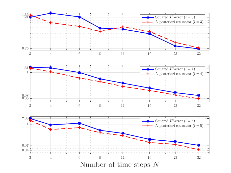
Refer to caption — Figure 1: Comparison between the squared $L^{2}$ -error and the a posteriori error estimator with different time steps and sample sizes (plotted in a log-log scale).

Figure 1 compares the squared $L^{2}$ -errors and the estimated squared errors (by using (5.6)) for numerical solutions obtained with 5 Picard iterations (i.e., $P=5$ ), and different time steps $N$ and sample sizes $\Lambda$ as listed in (5.7). We clearly observe that, for all choices of sample sizes, the convergence behavior of the estimated error and the true error are almost identical as the time stepsize tends to zero, which confirms the theoretical results in Theorem 4.2. Moreover, the ratio of the estimated error to the true error suggests that, for this set of model parameters, the generic equivalence constant in Theorem 4.2 lies within the range of $0.7-1.2$ , which indicates that the error estimator predicts the squared approximation error very accurately. By performing linear regression of the estimated values (the dashed line) against the number of time steps, we can infer without using the analytic solution of (5.1) that the approximation error (in the $L^{2}$ -norm) converges to zero at a rate of $N^{-0.7}$ for the cases $l=4,5$ , while for $l=3$ , the approximation error also converges to zero but with a much slower rate.

Note that for general decoupled FBSDEs, Corollary 1 in [23] suggests choosing the sample size $\Lambda$ corresponding to $l=5$ in the least-squares Monte Carlo method to achieve a half-order $L^{2}$ -convergence with respect to the number of time steps $N$ . Our numerical results indicate that, for the present example, the convergence behaviour is much better than this theoretical error estimate, possibly due to a better time regularity of the process $Z$ . This suggests that one can design more efficient algorithms with tailored hyper-parameters based on the error estimator (5.6). In particular, (5.6) shows that $l=4$ leads to the most efficient algorithm among the three choices of $l\in\{3,4,5\}$ . The cheaper algorithm with $l=3$ in general results in significantly larger errors, while the choice $l=5$ not only requires a tremendously higher computational cost, but also achieves almost the same accuracy as the choice $l=4$ for sufficiently fine grids; for instance, with $N=32$ time steps, the error estimator predicts increasing $l$ from $4$ to $5$ will only reduce the squared error from 0.0586 to 0.0427, and in fact the true squared error only reduces from 0.0822 to 0.0734. To illustrate the computational efforts for the two choices $l=4,5$ , we present the corresponding sample size $\Lambda$ and computational time with different numbers of time steps in Table 1.

Table 1: Sample size

\Lambda

and computational time with different

N

and

l

$l$	Sample size	Run time	Sample size	Run time
	$N=23$		$N=32$
4	32 768	533s	131 072	3 908s
5	370 728	5 715s	2 097 152	59 338s

We then proceed to examine the performance of the error estimator for MV-FBSDEs with stronger coupling, by varying the coefficient $1/c_{\alpha}\in\{0.7,1\}$ and keeping the other model parameters as above. Figure 2 (left) presents the numerical results obtained by the hybrid algorithm with 5 Picard iterations (i.e., $P=5$ ) and the discretization parameters $N,K,\Lambda$ as defined in (5.7) for $j=4,\ldots,9$ , $l=5$ . By comparison with the numerical results for $1/c_{a}=0.3$ (see Figure 1, bottom), we can clearly observe that as the coupling parameter $1/c_{a}$ increases, the same choice of discretization parameters leads to larger approximation errors. The $L^{2}$ -approximation error decays slowly for the case with $1/c_{\alpha}=0.7$ as the number of time steps $N$ tends to infinity, while for the case with $1/c_{\alpha}=1$ , the approximation errors oscillate around the value $10^{2}$ and do not show convergence for sufficiently large $N$ . Similar phenomena have been observed in [1, 16, 22], where the authors found that a stronger coupling between the forward and backward equations can pose significant numerical challenges such as slow convergence or even divergence of Picard iterations.

More importantly, we see that the performance of the a posteriori error estimator is very robust even for a large coupling parameter. Regardless of the convergence of the hybrid algorithm, the proposed error estimator captures the precise convergence behaviour of the true error starting from a fairly small number of time steps, and the ratio of the estimated error to the true error generally stays in the range of $0.7-1$ . This enables us to judge the success of a given choice of discretization parameters without knowing the analytic solution to the problem. In particular, the error estimator suggests that for the case with $1/c_{\alpha}\in\{0.7,1\}$ and $P=5$ , the dominating error stems from other sources (such as the Picard iteration) instead of the time discretization or the Monte Carlo regression. Hence we cannot expect to significantly improve the approximation accuracy by keeping the number of Picard iterations fixed and only by further refining the time grid or enlarging the sample size.

Motivated by the above observation, we carry out the hybrid algorithm with more Picard iterations ( $P=10$ for $1/c_{\alpha}=0.7$ and $P=20$ for $1/c_{\alpha}=1$ ) but less simulation samples ( $l=4$ ). Figure 2 (right) presents the numerical results for the discretization parameters $N,K,\Lambda$ as defined in (5.7) with $j=4,\ldots,9$ . One can observe a significant improvement in the algorithm’s efficiency for the case with $1/c_{\alpha}=0.7$ (see Figure 2, top-right), where the hybrid algorithm converges with a rate of $N^{-0.8}$ for the whole range of time steps, and results in more accurate numerical solutions with less computational time than the original choice of $P=5$ , $l=5$ (see Figure 2, top-left). The situation is less clear for the case with $1/c_{\alpha}=1$ (see Figure 2, bottom-right). Although the error is reduced by half as compared to the choice of $P=5$ and $l=5$ , the error estimator does not decrease significantly starting from $N=11$ , which suggests that more Picard iterations or a better scheme need to be employed for further improvements.⁵⁵ 5 Alternative approaches to decouple (2.1) include the fictitious play approach in [27] and the gradient descent approach in [40]. Rather than replacing the former iterate by the new one as in Picard iteration, these methods update the approximate solutions with a smaller rate to ensure the convergence of algorithms.

5.2 Multidimensional linear and nonlinear MV-FBSDEs

In this section, we demonstrate the effectiveness of the a posteriori estimator (1.2) for the following multidimensional coupled MV-FBSDEs: for all $t\in[0,T]$ ,

\displaystyle\begin{split}dX_{t}&=V_{t}\,dt,\quad dV_{t}=\bigg(\mathbb{E}[\kappa(x,v,X_{t},V_{t})]\big|_{(x,v)=(X_{t},V_{t})}-\frac{1}{2\gamma}Y^{2}_{t}\bigg)\,dt+\sigma\,dW_{t},\\ dY^{1}_{t}&=-\bigg(\mathbb{E}[\partial_{x}\kappa(x,v,X_{t},V_{t})]\big|_{(x,v)=(X_{t},V_{t})}Y^{2}_{t}+\mathbb{E}[\partial_{x^{\prime}}\kappa(X_{t},V_{t},x,v)Y^{2}_{t}]\big|_{(x,v)=(X_{t},V_{t})}\bigg)\,dt+Z^{1}_{t}\,dW_{t},\\ dY^{2}_{t}&=-\bigg(Y^{1}_{t}+\mathbb{E}[\partial_{v}\kappa(x,v,X_{t},V_{t})]\big|_{(x,v)=(X_{t},V_{t})}Y^{2}_{t}+\mathbb{E}[\partial_{v^{\prime}}\kappa(X_{t},V_{t},x,v)Y^{2}_{t}]\big|_{(x,v)=(X_{t},V_{t})}\\ &\quad+2(V_{t}-\mathbb{E}[V_{t}])\bigg)\,dt+Z^{2}_{t}\,dW_{t},\\ X_{0}&=x_{0},\quad V_{0}=v_{0},\quad Y^{1}_{T}=0,\quad Y^{2}_{T}=2(V_{T}-\mathbb{E}[V_{T}]),\end{split}

(5.8)

where $T>0$ , $n\in\mathbb{N}$ , $\gamma>0$ and $\sigma\in\mathbb{R}^{n\times n}$ are given constants, $x_{0},v_{0}$ are given $\mathbb{R}^{n}$ -valued square integrable random variables, $W$ is an $n$ -dimensional standard Brownian motion, $\kappa:\mathbb{R}^{n}\times\mathbb{R}^{n}\times\mathbb{R}^{n}\times\mathbb{R}^{n}\rightarrow\mathbb{R}^{n}$ is the interaction kernel given by

\kappa(x,v,x^{\prime},v^{\prime})=\frac{v^{\prime}-v}{(1+|x-x^{\prime}|^{2})^{\beta}},\quad\textnormal{with some given $\beta\geq 0$,}

(5.9)

and $X,V,Y^{1},Y^{2},Z^{1},Z^{2}$ are unknown $n$ -dimensional solution processes. The equation (5.8) arises from applying the Pontryagin maximum principle to an optimal control problem of multidimensional stochastic mean-field Cucker–Smale dynamics, where the controller applies an external force to induce a consensus of the velocity process $V$ (i.e., all trajectories of the velocity process tend to the same value as $t$ increases). We refer the reader to [40, Section 5.2] for details of the control problem and to [2, 35, 10, 27] for similar control problems.

If $\beta=0$ in (5.9), then (5.8) reduces to a linear MV-FBSDE, which satisfies (H.1) and (H.2). For $\beta>0$ , the coefficients of (5.8) exhibit a more complicated interaction through the nonlinear kernel (5.9). The coupling strength of the forward and backward dynamics in (5.8) is determined by the parameter $\gamma$ , i.e., the smaller the parameter $\gamma$ , the stronger the coupling. In the sequel, we fix $T=1$ , $\sigma=0.1\mathbb{I}_{n}$ and $(x_{0},v_{0})\sim\textrm{Unif}([0,1]^{2n})$ , and examine the performance of (1.2) for different choices of $\gamma,\beta>0$ and $n\in\mathbb{N}$ . As we shall see soon, although (H.1) may not hold for general $\beta,\gamma>0$ , the error estimator (1.2) still quantifies the approximation errors very well.

Two-dimensional nonlinear examples.

We first carry out the experiments with $n=1$ , $\gamma=0.3$ and $\beta\in\{1,10\}$ . For any given $\beta$ , we compute approximate solutions to the two-dimensional MV-FBSDE (5.8) by the deep BSDE method introduced in (4.7). More precisely, we use a neural network $f_{\theta}:\mathbb{R}^{2}\rightarrow\mathbb{R}^{2}$ (with one hidden layer of width 20 and the sigmoid activation function) to approximate the decoupling field of $(Y_{0}^{1},Y_{0}^{2})$ , and use a neural network $g_{\vartheta}:\mathbb{R}^{3}\rightarrow\mathbb{R}^{2}$ (with one hidden layer of width 110 and the sigmoid activation function) to approximate the decoupling fields of $(Z^{1},Z^{2})$ at all times. We then take a uniform grid $\pi$ of $[0,1]$ with stepsize $1/32$ , and compute the discrete solution $\hat{\Theta}=(\hat{X},\hat{V},\hat{Y}^{1},\hat{Y}^{2},\hat{Z}^{1},\hat{Z}^{2})$ of (5.8) using the explicit forward Euler scheme (4.7) on the grid $\pi$ . Note that the discrete solution $\hat{\Theta}$ depends on the network parameters $(\theta,\vartheta)$ , which we update iteratively by minimising the following terminal loss:

\mathcal{E}_{\pi}(\hat{\Theta})={\mathbb{E}}[|\hat{Y}^{1}_{N}|^{2}]+{\mathbb{E}}[|\hat{Y}^{2}_{N}-2(\hat{V}_{N}-\mathbb{E}[\hat{V}_{N}])|^{2}].

(5.10)

For each iteration, we consider a particle approximation of size $500$ to (5.8), estimate the law $\mathbb{P}_{\hat{\Theta}}$ via its empirical distribution, and update the network parameters with the Adam algorithm. This yields a sequence of parameters $(\theta_{\ell},\vartheta_{\ell})_{\ell\in\mathbb{N}}$ , which in turn yields a sequence of approximate solutions $(\hat{\Theta}^{\ell})_{\ell\in\mathbb{N}}$ to (5.8).

To assess the accuracy of $(\hat{\Theta}^{\ell})_{\ell\in\mathbb{N}}$ , we obtain a reference solution using the iterative PDE method introduced in [40, Section 5.2], as the exact solution to (5.8) is not known.⁶⁶ 6 For the PDE method, we choose the computational domain $[-1,3]^{2}$ , time stepsize $1/64$ and mesh size $1/100$ , which lead to negligible discretization errors on the basis of our experiments. This allows for computing the squared approximation errors of $(\hat{\Theta}^{\ell})_{\ell\in\mathbb{N}}$ defined in (4.2). We shall compare the approximation error of $\hat{\Theta}^{\ell}$ with the predicted error given by the error estimator (1.2), which simplifies to the terminal loss (5.10), and is estimated by a particle approximation of size $5000$ .

Figure 3 compares the squared $L^{2}$ -error of numerical solutions with the estimated error from the error estimator (1.2), for different values of $\beta$ and Adam iterations. It can be observed that the error estimator tracks the true error well starting from a fairly small number of Adam iterations. The ratio of the estimated error to the true error consistently falls within the range of $0.6-0.8$ throughout all iterations, and is robust to the changes in the value of $\beta$ . This suggests that the estimator provides a reliable measure of the approximation error.

High dimensional linear examples.

We then perform experiments with $\beta=0$ , $\gamma\in\{0,2,0.3,0.5\}$ and $n\in\{3,6,9\}$ . As $\beta=0$ , the interaction kernel $\kappa$ in (5.9) is independent of $x$ and $x^{\prime}$ , which along with $Y^{2}_{T}=0$ implies that $Y^{1}_{t}=Z^{1}_{t}=0$ for all $t\in[0,T]$ . Moreover, by the linearity of $\kappa$ in $v$ and $v^{\prime}$ and the terminal condition of $Y^{2}$ , one can show by Itô’s formula that

Y_{t}^{2}=\alpha_{t}(V_{t}-\mathbb{E}[V_{t}]),\quad Z_{t}^{2}=\sigma\alpha_{t},\quad t\in[0,T],

(5.11)

where $\alpha:[0,T]\rightarrow\mathbb{R}$ satisfies $a^{\prime}_{t}-2a_{t}-\frac{1}{2\gamma}a_{t}^{2}+2=0$ with $a_{T}=2$ . This provides a reference solution against which the accuracy of the given approximate solutions can be evaluated.

In the sequel, for each $n$ and $\gamma$ , we focus on solving the processes $V$ , $Y^{2}$ and $Z^{2}$ , since the processes $(Y^{1},Z^{1})$ are zero, and the process $X$ can be obtained by integrating $V$ in time. This reduces (5.8) to an $n$ -dimensional linear MV-FBSDE, which we solve using the deep BSDE method described above. In particular, we approximate $Y^{2}_{0}$ and $(Z^{2})_{t\in[0,T]}$ by

Y^{2}_{0}\approx f_{\theta}(V_{0}),\quad Z^{2}_{t}\approx g_{\vartheta}(t,V_{t}),\quad t\in[0,T],

where $f_{\theta}:\mathbb{R}^{n}\rightarrow\mathbb{R}^{n}$ and $g_{\vartheta}:\mathbb{R}^{n+1}\rightarrow\mathbb{R}^{n}$ are neural networks with the sigmoid activation function and 1 hidden layer of widths 20 and 110, respectively. The network parameters $(\theta,\vartheta)$ are updated by applying the Adam algorithm to minimize the terminal loss:

\mathcal{E}_{\pi}(\hat{\Theta})={\mathbb{E}}[|\hat{Y}^{2}_{N}-2(\hat{V}_{N}-\mathbb{E}[\hat{V}_{N}])|^{2}].

(5.12)

The other discretisation parameters, such as the time grid for the forward Euler scheme (4.7) and the size of the particle system for each Adam iteration, are chosen as in the above two-dimensional setting. For any given numerical solution $(\hat{V},\hat{Y}^{2},\hat{Z}^{2})$ , the a posteriori error estimator (5.10) is estimated by a particle approximation of size $5000$ , and the squared $L^{2}$ -error is computed using the reference solution given in (5.11).

Figure 4(a) compares the squared $L^{2}$ -error of numerical solutions with the a posteriori error estimator, for $n=3$ , and different values of $\gamma\in\{0.2,0.3,0.5\}$ and Adam iterations. The results show that the estimated error and the true error have almost identical convergence behaviour. Moreover, as the number of iterations increases, the ratio of the estimated error to the true error decreases, indicating that the error estimator predicts the approximation error more accurately. One may also observe a slight increase of the estimation ratio as $\gamma$ approaches $0$ . Specifically, over the last 150 iterations, the estimation ratios for $\gamma=0.5$ lie in the range of $0.92-1.05$ , whereas the estimation ratios for $\gamma=0.2$ lie in the range of $1.38-2$ . This suggests the generic equivalence constant in Theorem 4.2 may increase as the coupling between the forward and backward equations becomes stronger.

Figure 4(b) investigates the impact of the problem dimension $n$ on the performance of the a posteriori error estimator. As the dimensionality increases, the squared $L^{2}$ -error increases linearly, and the Adam algorithm requires more iterations to achieve the same level of accuracy. Despite this dependence on dimensionality, the ratio of the estimated error to the true error remains stable. As the number of iterations increases, the estimation ratios decrease and eventually stabilize within the range of $1-1.5$ . This indicates that the a posteriori error estimator is a reliable tool for assessing the accuracy of numerical solutions in high-dimensional problems.

Appendix A Proofs of technical results

A.1 Proofs of Proposition 2.1 and Lemma 2.3

We first recall the discrete Gronwall Lemma given in [29].

Lemma A.1.

Let $\{y_{n}\}_{n\in\mathbb{N}\cup\{0\}}$ and $\{g_{n}\}_{n\in\mathbb{N}\cup\{0\}}$ be sequences of nonnegative real numbers, and $c\geq 0$ . If $y_{n}\leq c+\sum_{k=0}^{n-1}g_{k}y_{k}$ for all $n\in\mathbb{N}\cup\{0\}$ , then

\max_{k=1,\ldots n}y_{k}\leq c\exp\left(\sum_{k=0}^{n-1}g_{k}\right),\quad\forall n\in\mathbb{N}\cup\{0\}.

We then establish a preparatory lemma for Proposition 2.1.

Lemma A.2.

Suppose the generator $(b,\sigma,f,g)$ satisfies (H.1), and the generator $(\bar{b},\bar{\sigma},\bar{f},\bar{g})$ satisfies (H.1 3). Let $\alpha,\beta_{1},\beta_{2}$ and $G$ be the constants in (H.1 1), $L$ be the constant in (H.1 2), $N\in{\mathbb{N}}$ , $\lambda_{0}\in[0,1]$ , let $(\phi,\psi,\gamma),(\bar{\phi},\bar{\psi},\bar{\gamma})\in\mathcal{M}^{2}(0,T;{\mathbb{R}}^{n}\times{\mathbb{R}}^{n\times d}\times{\mathbb{R}}^{m})$ , $\eta,\bar{\eta}\in L^{2}(\mathcal{F}_{T};{\mathbb{R}}^{m})$ , $\xi_{0},\bar{\xi}_{0}\in L^{2}(\mathcal{F}_{0};{\mathbb{R}}^{m})$ , let $(X,Y,Z,M)\in\mathcal{S}_{N}$ (resp. $(\bar{X},\bar{Y},\bar{Z},\bar{M})\in\mathcal{S}_{N}$ ) satisfy (2.3) defined on $\pi_{N}$ corresponding to $\lambda=\lambda_{0}$ , the generator $(b,\sigma,f,g)$ and $(\phi,\psi,\gamma,\eta,\xi_{0})$ (resp. the generator $(\bar{b},\bar{\sigma},\bar{f},\bar{g})$ and $(\bar{\phi},\bar{\psi},\bar{\gamma},\bar{\eta},\bar{\xi}_{0})$ ), and let $(\delta X,\delta Y,\delta Z)=(X-\bar{X},Y-\bar{Y},Z-\bar{Z})$ , $(\delta\phi,\delta\psi,\delta\gamma,\delta\eta,\delta\xi_{0})=(\phi-\bar{\phi},\psi-\bar{\psi},\gamma-\bar{\gamma},\eta-\bar{\eta},\xi_{0}-\bar{\xi}_{0})$ . Then it holds for all $\varepsilon_{1},\varepsilon_{2},\varepsilon_{3}>0$ that

\displaystyle\begin{split}&\min\{1,\alpha\}{\mathbb{E}}[|G\delta X_{N}|^{2}]+\sum_{i=0}^{N-1}{\mathbb{E}}[\beta_{2}|G\delta X_{i}|^{2}+\beta_{1}(|G^{*}\delta Y_{i}|^{2}+|G^{*}\delta Z_{i}|^{2})]\tau_{N}\\ &\leq\varepsilon_{1}{\mathbb{E}}[|G^{*}\delta Y_{0}|^{2}]+\frac{1}{4\varepsilon_{1}}{\mathbb{E}}[|\delta\xi_{0}|^{2}]+\varepsilon_{2}{\mathbb{E}}[|G\delta X_{N}|^{2}]+\frac{1}{4\varepsilon_{2}}{\mathbb{E}}[|\lambda_{0}(g(\bar{X}_{N},\mathbb{P}_{\bar{X}_{N}})-\bar{g}(\bar{X}_{N},\mathbb{P}_{\bar{X}_{N}}))+\delta\eta|^{2}]\\ &\quad+\sum_{i=0}^{N-1}{\mathbb{E}}\bigg[\varepsilon_{2}|G\delta X_{i}|^{2}+\varepsilon_{3}(|G^{*}\delta Y_{i}|^{2}+|G^{*}\delta{Z}_{i}|^{2})+\bigg(\frac{1}{4\varepsilon_{2}}+\tau_{N}\bigg)|\lambda_{0}(\hat{f}(t_{i})-\bar{f}(t_{i}))+\delta\gamma_{i}|^{2}\\ &\quad+\bigg(\frac{1}{4\varepsilon_{3}}+\tau_{N}\|G\|^{2}\bigg)|\lambda_{0}(\hat{b}(t_{i})-\bar{b}(t_{i}))+\delta\phi_{i}|^{2}+\frac{1}{4\varepsilon_{3}}|\lambda_{0}(\hat{\sigma}(t_{i})-\bar{\sigma}(t_{i}))+\delta\psi_{i}|^{2}\bigg]\tau_{N}\\ &\quad+C_{(G,\beta_{1},\beta_{2},L)}\sum_{i=0}^{N-1}{\mathbb{E}}[|\delta X_{i}|^{2}+|\delta Y_{i}|^{2}+|\delta{Z}_{i}|^{2}]\tau^{2}_{N},\end{split}

where $C_{(G,\beta_{1},\beta_{2},L)}$ is a constant depending only on $G,\beta_{1},\beta_{2},L$ , and for each $i\in\mathcal{N}$ , $\phi=b,\sigma,f$ , we define $\hat{\phi}(t_{i})\coloneqq\phi(t_{i},\bar{X}_{i},\bar{Y}_{i},\bar{Z}_{i},\mathbb{P}_{(\bar{X}_{i},\bar{Y}_{i},\bar{Z}_{i})})$ and $\bar{\phi}(t_{i})\coloneqq\bar{\phi}(t_{i},\bar{X}_{i},\bar{Y}_{i},\bar{Z}_{i},\mathbb{P}_{(\bar{X}_{i},\bar{Y}_{i},\bar{Z}_{i})})$ .

Proof of Lemma A.2.

Throughout this proof, for each $\lambda\in[0,1]$ and $(t,x,y,z,\mu,\nu)\in[0,1]\times{\mathbb{R}}^{n}\times{\mathbb{R}}^{m}\times{\mathbb{R}}^{m\times d}\times\mathcal{P}_{2}({\mathbb{R}}^{n+m+md})\times\mathcal{P}_{2}({\mathbb{R}}^{n})$ let $b^{\lambda}(t,x,y,z,\mu)=(1-\lambda)\beta_{1}(-G^{*}y)+\lambda b(t,x,y,z,\mu)$ , $\sigma^{\lambda}(t,x,y,z,\mu)=(1-\lambda)\beta_{1}(-G^{*}z)+\lambda\sigma(t,x,y,z,\mu)$ , $f^{\lambda}(t,x,y,z,\mu)=(1-\lambda)\beta_{2}Gx+\lambda f(t,x,y,z,\mu)$ and $g^{\lambda}(x,\nu)=(1-\lambda)Gx+\lambda g(x,\nu)$ . Let $\Theta=(X,Y,Z)$ , $\bar{\Theta}=(\bar{X},\bar{Y},\bar{Z})$ , $(\delta\Theta,\delta X,\delta Y,\delta Z,\delta M)=(\Theta-\bar{\Theta},X-\bar{X},Y-\bar{Y},Z-\bar{Z},M-\bar{M})$ , for each $t\in[0,T]$ , $h=b,\sigma,f,b^{\lambda},\sigma^{\lambda},f^{\lambda}$ let ${h}(t)=h(t,{\Theta}_{t},\mathbb{P}_{{\Theta}_{t}})$ , $\hat{h}(t)=h(t,\bar{\Theta}_{t},\mathbb{P}_{\bar{\Theta}_{t}})$ , $\delta{h}(t)=h(t)-\hat{h}(t)$ and $\bar{h}(t)=\bar{h}(t,\bar{\Theta}_{t},\mathbb{P}_{\bar{\Theta}_{t}})$ .

Note that we can deduce from (2.3) that $\delta X_{0}=\delta\xi_{0}$ , $\delta Y_{N}=g^{\lambda_{0}}(X_{N},\mathbb{P}_{X_{N}})-\bar{g}^{\lambda_{0}}(\bar{X}_{N},\mathbb{P}_{\bar{X}_{N}})+\delta\eta$ , and for any given $i\in\mathcal{N}_{<N}$ that

	$\displaystyle\Delta(\delta{X})_{i}$	$\displaystyle=(b^{\lambda_{0}}(t_{i})-\bar{b}^{\lambda_{0}}(t_{i})+\delta\phi_{i})\tau_{N}+(\sigma^{\lambda_{0}}(t_{i})-\bar{\sigma}^{\lambda_{0}}(t_{i})+\delta\psi_{i})\,\Delta W_{i}$		(A.1)
	$\displaystyle\Delta(\delta{Y})_{i}$	$\displaystyle=-[f^{\lambda_{0}}(t_{i})-\bar{f}^{\lambda_{0}}(t_{i})+\delta\gamma_{i}]\tau_{N}+\delta{Z}_{i}\,\Delta W_{i}+\Delta(\delta{M})_{i},$		(A.2)

which together with the definition of the backward operator $\Delta$ shows for all $i\in\mathcal{N}_{<N}$ that

\displaystyle\begin{split}\Delta\langle G\delta X,\delta Y\rangle_{i}&=\langle G\Delta(\delta X)_{i},(\delta Y)_{i}\rangle+\langle G(\delta X)_{i},\Delta(\delta Y)_{i}\rangle+\langle G\Delta(\delta X)_{i},\Delta(\delta Y)_{i}\rangle\\ &=\langle G[(b^{\lambda_{0}}(t_{i})-\bar{b}^{\lambda_{0}}(t_{i})+\delta\phi_{i})\tau_{N}+(\sigma^{\lambda_{0}}(t_{i})-\bar{\sigma}^{\lambda_{0}}(t_{i})+\delta\psi_{i})\,\Delta W_{i}],(\delta Y)_{i}\rangle\\ &\quad+\langle G(\delta X)_{i},-[f^{\lambda_{0}}(t_{i})-\bar{f}^{\lambda_{0}}(t_{i})+\delta\gamma_{i}]\tau_{N}+\delta{Z}_{i}\,\Delta W_{i}+\Delta(\delta{M})_{i}\rangle\\ &\quad+\langle G[(b^{\lambda_{0}}(t_{i})-\bar{b}^{\lambda_{0}}(t_{i})+\delta\phi_{i})\tau_{N}],-[f^{\lambda_{0}}(t_{i})-\bar{f}^{\lambda_{0}}(t_{i})+\delta\gamma_{i}]\tau_{N}\rangle\\ &\quad+\langle G[(b^{\lambda_{0}}(t_{i})-\bar{b}^{\lambda_{0}}(t_{i})+\delta\phi_{i})\tau_{N}],\delta{Z}_{i}\,\Delta W_{i}+\Delta(\delta{M})_{i}\rangle\\ &\quad+\langle G[(\sigma^{\lambda_{0}}(t_{i})-\bar{\sigma}^{\lambda_{0}}(t_{i})+\delta\psi_{i})\,\Delta W_{i}],-[f^{\lambda_{0}}(t_{i})-\bar{f}^{\lambda_{0}}(t_{i})+\delta\gamma_{i}]\tau_{N}+\Delta(\delta{M})_{i}\rangle\\ &\quad+\langle G[(\sigma^{\lambda_{0}}(t_{i})-\bar{\sigma}^{\lambda_{0}}(t_{i})+\delta\psi_{i})\,\Delta W_{i}],\delta{Z}_{i}\,\Delta W_{i}\rangle.\end{split}

Then, adding and subtracting the terms $\hat{b}^{\lambda_{0}}(t_{i})$ , $\hat{\sigma}^{\lambda_{0}}(t_{i})$ and $\hat{f}^{\lambda_{0}}(t_{i})$ imply for all $i\in\mathcal{N}_{<N}$ that

\displaystyle\begin{split}&\Delta\langle G\delta X,\delta Y\rangle_{i}\\ &=\langle G[(\delta b^{\lambda_{0}}(t_{i})+\hat{b}^{\lambda_{0}}(t_{i})-\bar{b}^{\lambda_{0}}(t_{i})+\delta\phi_{i})\tau_{N}+(\sigma^{\lambda_{0}}(t_{i})-\bar{\sigma}^{\lambda_{0}}(t_{i})+\delta\psi_{i})\,\Delta W_{i}],(\delta Y)_{i}\rangle\\ &\quad+\langle G(\delta X)_{i},-[\delta f^{\lambda_{0}}(t_{i})+\hat{f}^{\lambda_{0}}(t_{i})-\bar{f}^{\lambda_{0}}(t_{i})+\delta\gamma_{i}]\tau_{N}+\delta{Z}_{i}\,\Delta W_{i}+\Delta(\delta{M})_{i}\rangle\\ &\quad+\langle G[(\delta b^{\lambda_{0}}(t_{i})+\hat{b}^{\lambda_{0}}(t_{i})-\bar{b}^{\lambda_{0}}(t_{i})+\delta\phi_{i})\tau_{N}],-[\delta f^{\lambda_{0}}(t_{i})+\hat{f}^{\lambda_{0}}(t_{i})-\bar{f}^{\lambda_{0}}(t_{i})+\delta\gamma_{i}]\tau_{N}\rangle\\ &\quad+\langle G[(b^{\lambda_{0}}(t_{i})-\bar{b}^{\lambda_{0}}(t_{i})+\delta\phi_{i})\tau_{N}],\delta{Z}_{i}\,\Delta W_{i}+\Delta(\delta{M})_{i}\rangle\\ &\quad+\langle G[(\sigma^{\lambda_{0}}(t_{i})-\bar{\sigma}^{\lambda_{0}}(t_{i})+\delta\psi_{i})\,\Delta W_{i}],-[f^{\lambda_{0}}(t_{i})-\bar{f}^{\lambda_{0}}(t_{i})+\delta\gamma_{i}]\tau_{N}+\Delta(\delta{M})_{i}\rangle\\ &\quad+\langle G[(\delta\sigma^{\lambda_{0}}(t_{i})+\hat{\sigma}^{\lambda_{0}}(t_{i})-\bar{\sigma}^{\lambda_{0}}(t_{i})+\delta\psi_{i})\,\Delta W_{i}],\delta{Z}_{i}\,\Delta W_{i}\rangle.\end{split}

By further introducing the following residual terms $\Phi_{i}$ , $\Psi_{i}$ and $\Sigma_{i}$ :

	$\displaystyle\Phi_{i}$	$\displaystyle=\langle G[(\sigma^{\lambda_{0}}(t_{i})-\bar{\sigma}^{\lambda_{0}}(t_{i})+\delta\psi_{i})\,\Delta W_{i}],(\delta Y)_{i}\rangle+\langle G(\delta X)_{i},\delta{Z}_{i}\,\Delta W_{i}+\Delta(\delta{M})_{i}\rangle$
		$\displaystyle\quad+\langle G[(b^{\lambda_{0}}(t_{i})-\bar{b}^{\lambda_{0}}(t_{i})+\delta\phi_{i})\tau_{N}],\delta{Z}_{i}\,\Delta W_{i}+\Delta(\delta{M})_{i}\rangle$
		$\displaystyle\quad+\langle G[(\sigma^{\lambda_{0}}(t_{i})-\bar{\sigma}^{\lambda_{0}}(t_{i})+\delta\psi_{i})\,\Delta W_{i}],-[f^{\lambda_{0}}(t_{i})-\bar{f}^{\lambda_{0}}(t_{i})+\delta\gamma_{i}]\tau_{N}+\Delta(\delta{M})_{i}\rangle,$
	$\displaystyle\Psi_{i}$	$\displaystyle=\langle G[(\hat{b}^{\lambda_{0}}(t_{i})-\bar{b}^{\lambda_{0}}(t_{i})+\delta\phi_{i})\tau_{N}],(\delta Y)_{i}\rangle+\langle G(\delta X)_{i},-[\hat{f}^{\lambda_{0}}(t_{i})-\bar{f}^{\lambda_{0}}(t_{i})+\delta\gamma_{i}]\tau_{N}\rangle$
		$\displaystyle\quad+\langle G[(\hat{\sigma}^{\lambda_{0}}(t_{i})-\bar{\sigma}^{\lambda_{0}}(t_{i})+\delta\psi_{i})\,\Delta W_{i}],\delta{Z}_{i}\,\Delta W_{i}\rangle,$
	$\displaystyle\Sigma_{i}$	$\displaystyle=\langle G[(\delta b^{\lambda_{0}}(t_{i})+\hat{b}^{\lambda_{0}}(t_{i})-\bar{b}^{\lambda_{0}}(t_{i})+\delta\phi_{i})\tau_{N}],-[\delta f^{\lambda_{0}}(t_{i})+\hat{f}^{\lambda_{0}}(t_{i})-\bar{f}^{\lambda_{0}}(t_{i})+\delta\gamma_{i}]\tau_{N}\rangle,$

we have for all $i\in\mathcal{N}_{<N}$ that

\displaystyle\begin{split}\Delta\langle G\delta X,\delta Y\rangle_{i}&=\langle\delta b^{\lambda_{0}}(t_{i})\tau_{N},G^{*}(\delta Y)_{i}\rangle+\langle G(\delta X)_{i},-\delta f^{\lambda_{0}}(t_{i})\tau_{N}\rangle\\ &\quad+\langle G\delta\sigma^{\lambda_{0}}(t_{i})\,\Delta W_{i},\delta{Z}_{i}\,\Delta W_{i}\rangle+\Phi_{i}+\Psi_{i}+\Sigma_{i}.\end{split}

We then compute ${\mathbb{E}}[\Delta\langle G\delta X,\delta Y\rangle_{i}]$ . By using the definition of the backward operator $\Delta$ , and the fact that $M$ , $\bar{M}$ are strongly orthogonal to $W$ , we see ${\mathbb{E}}_{i}[\Delta(\delta M)_{i}(\Delta W_{i})^{*}]=0$ for all $i\in\mathcal{N}_{<N}$ . Thus, we can deduce from the adaptedness of the coefficients and the law of iterated expectations that ${\mathbb{E}}[\Phi_{i}]=0$ . Moreover, the property that ${\mathbb{E}}_{i}[\Delta W_{i}(\Delta W_{i})^{*}]=\tau_{N}{\mathbb{I}}_{d}$ implies that

{\mathbb{E}}_{i}[\langle G\delta\sigma^{\lambda_{0}}(t_{i})\Delta W_{i},\delta Z_{i}\Delta W_{i}\rangle]={\mathbb{E}}_{i}[\textnormal{tr}(\Delta W_{i}(\Delta W_{i})^{*}(G\delta\sigma^{\lambda_{0}}(t_{i}))^{*}\delta Z_{i})]=\tau_{N}{\mathbb{E}}_{i}[\langle\delta\sigma^{\lambda_{0}}(t_{i}),G^{*}\delta Z_{i})\rangle],

where we have used the fact that the trace commutes with conditional expectations. Consequently, for each $i\in\mathcal{N}_{<N}$ , we have that

	$\displaystyle{\mathbb{E}}[\Delta\langle G\delta X,\delta Y\rangle_{i}]$	$\displaystyle=\tau_{N}{\mathbb{E}}[\langle\delta\sigma^{\lambda_{0}}(t_{i}),G^{}\delta Z_{i}\rangle+\langle\delta b^{\lambda_{0}}(t_{i}),G^{}\delta Y_{i}\rangle+\langle-\delta f^{\lambda_{0}}(t_{i}),G\delta X_{i}\rangle]$
		$\displaystyle\quad+{\mathbb{E}}[\Psi_{i}]+{\mathbb{E}}[\Sigma_{i}],$

where we can deduce from the definitions of $(\hat{b}^{\lambda_{0}},\hat{\sigma}^{\lambda_{0}},\hat{f}^{\lambda_{0}},\hat{g}^{\lambda_{0}})$ and $(\bar{b}^{\lambda_{0}},\bar{\sigma}^{\lambda_{0}},\bar{f}^{\lambda_{0}},\bar{g}^{\lambda_{0}})$ that

$\displaystyle{\mathbb{E}}[\Psi_{i}]$	$\displaystyle=\tau_{N}{\mathbb{E}}\big[\langle\lambda_{0}(\hat{b}(t_{i})-\bar{b}(t_{i}))+\delta\phi_{i},G^{*}\delta Y_{i}\rangle+\langle G(\delta X)_{i},-[{\lambda_{0}}(\hat{f}(t_{i})-\bar{f}(t_{i}))+\delta\gamma_{i}]\rangle$
	$\displaystyle\quad+\langle{\lambda_{0}}(\hat{\sigma}(t_{i})-\bar{\sigma}(t_{i}))+\delta\psi_{i},G^{*}\delta{Z}_{i}\rangle\big],$	(A.3)
$\displaystyle{\mathbb{E}}[\Sigma_{i}]$	$\displaystyle=\tau_{N}^{2}{\mathbb{E}}\big[\langle G[\delta b^{\lambda_{0}}(t_{i})+{\lambda_{0}}(\hat{b}(t_{i})-\bar{b}(t_{i}))+\delta\phi_{i}],-[\delta f^{\lambda_{0}}(t_{i})+{\lambda_{0}}(\hat{f}(t_{i})-\bar{f}(t_{i}))+\delta\gamma_{i}]\rangle\big].$	(A.4)

Note that for each $\lambda\in[0,1)$ , the coefficients $(b^{\lambda},\sigma^{\lambda},-f^{\lambda})$ satisfy (H.1 1) with the same $G,\beta_{1},\beta_{2}$ . Hence, by summing the above identity over the index $i$ from $0$ to $N-1$ and applying the monotonicity condition (H.1 1), we have that

		$\displaystyle{\mathbb{E}}[\langle G\delta X_{N},\delta Y_{N}\rangle]-{\mathbb{E}}[\langle G\delta X_{0},\delta Y_{0}\rangle]$
		$\displaystyle=\sum_{i=0}^{N-1}\tau_{N}{\mathbb{E}}[\langle-\delta f^{\lambda_{0}}(t_{i}),G\delta X_{i}\rangle+\langle\delta\sigma^{\lambda_{0}}(t_{i}),G^{}\delta Z_{i}\rangle+\langle\delta b^{\lambda_{0}}(t_{i}),G^{}\delta Y_{i}\rangle]+{\mathbb{E}}[\Psi_{i}]+{\mathbb{E}}[\Sigma_{i}]$
		$\displaystyle\leq\sum_{i=0}^{N-1}\tau_{N}{\mathbb{E}}[-\beta_{2}\|G\delta X_{i}\|^{2}-\beta_{1}(\|G^{}\delta Z_{i}\|^{2}+\|G^{}\delta Y_{i}\|^{2})]+\sum_{i=0}^{N-1}({\mathbb{E}}[\Psi_{i}]+{\mathbb{E}}[\Sigma_{i}]).$

Then by rearranging the terms and using the fact that $(\delta X)_{0}=\delta\xi_{0}$ ,

\displaystyle\delta Y_{N}

\displaystyle=g^{\lambda_{0}}(X_{N},\mathbb{P}_{X_{N}})-g^{\lambda_{0}}(\bar{X}_{N},\mathbb{P}_{\bar{X}_{N}})+g^{\lambda_{0}}(\bar{X}_{N},\mathbb{P}_{\bar{X}_{N}})-\bar{g}^{\lambda_{0}}(\bar{X}_{N},\mathbb{P}_{\bar{X}_{N}})+\delta\eta,

and the monotonicity of $g$ , we arrive at the estimate that

		$\displaystyle(1-\lambda_{0}+\lambda_{0}\alpha){\mathbb{E}}[\|G\delta X_{N}\|^{2}]+\sum_{i=0}^{N-1}{\mathbb{E}}[\beta_{2}\|G\delta X_{i}\|^{2}+\beta_{1}(\|G^{}\delta Y_{i}\|^{2}+\|G^{}\delta Z_{i}\|^{2})]\tau_{N}$
		$\displaystyle\leq{\mathbb{E}}[\langle G\delta\xi_{0},\delta Y_{0}\rangle]-{\mathbb{E}}[\langle G\delta X_{N},g^{\lambda_{0}}(\bar{X}_{N},\mathbb{P}_{\bar{X}_{N}})-\bar{g}^{\lambda_{0}}(\bar{X}_{N},\mathbb{P}_{\bar{X}_{N}})+\delta\eta\rangle]+\sum_{i=0}^{N-1}({\mathbb{E}}[\Psi_{i}]+{\mathbb{E}}[\Sigma_{i}]),$

which together with the fact that $(1-\lambda_{0}+\lambda_{0}\alpha)\geq\min\{1,\alpha\}$ , (A.3) and Young’s inequality implies for all $\varepsilon_{1},\varepsilon_{2},\varepsilon_{3}>0$ that

\displaystyle\begin{split}&\min\{1,\alpha\}{\mathbb{E}}[|G\delta X_{N}|^{2}]+\sum_{i=0}^{N-1}{\mathbb{E}}[\beta_{2}|G\delta X_{i}|^{2}+\beta_{1}(|G^{*}\delta Z_{i}|^{2}+|G^{*}\delta Y_{i}|^{2})]\tau_{N}\\ &\leq\varepsilon_{1}{\mathbb{E}}[|G^{*}\delta Y_{0}|^{2}]+\frac{1}{4\varepsilon_{1}}{\mathbb{E}}[|\delta\xi_{0}|^{2}]+\varepsilon_{2}{\mathbb{E}}[|G\delta X_{N}|^{2}]+\frac{1}{4\varepsilon_{2}}{\mathbb{E}}[|\lambda_{0}(g(\bar{X}_{N},\mathbb{P}_{\bar{X}_{N}})-\bar{g}(\bar{X}_{N},\mathbb{P}_{\bar{X}_{N}}))+\delta\eta|^{2}]\\ &\quad+\sum_{i=0}^{N-1}{\mathbb{E}}\bigg[\varepsilon_{2}|G\delta X_{i}|^{2}+\varepsilon_{3}(|G^{*}\delta Y_{i}|^{2}+|G^{*}\delta{Z}_{i}|^{2})+\frac{1}{4\varepsilon_{2}}|\lambda_{0}(\hat{f}(t_{i})-\bar{f}(t_{i}))+\delta\gamma_{i}|^{2}\\ &\quad+\frac{1}{4\varepsilon_{3}}\bigg(|\lambda_{0}(\hat{b}(t_{i})-\bar{b}(t_{i}))+\delta\phi_{i}|^{2}+|\lambda_{0}(\hat{\sigma}(t_{i})-\bar{\sigma}(t_{i}))+\delta\psi_{i}|^{2}\bigg)\bigg]\tau_{N}+\sum_{i=0}^{N-1}{\mathbb{E}}[\Sigma_{i}].\end{split}

Finally, it remains to estimate $\sum_{i=0}^{N-1}{\mathbb{E}}[\Sigma_{i}]$ . We obtain from (A.4) and Young’s inequality that

	$\displaystyle{\mathbb{E}}[\Sigma_{i}]$	$\displaystyle=\tau_{N}^{2}{\mathbb{E}}\big[\langle G[\delta b^{\lambda_{0}}(t_{i})+{\lambda_{0}}(\hat{b}(t_{i})-\bar{b}(t_{i}))+\delta\phi_{i}],-[\delta f^{\lambda_{0}}(t_{i})+{\lambda_{0}}(\hat{f}(t_{i})-\bar{f}(t_{i}))+\delta\gamma_{i}]\rangle\big]$
		$\displaystyle\leq\tau_{N}^{2}\bigg({\mathbb{E}}\big[\\|G\\|^{2}\|\delta b^{\lambda_{0}}(t_{i})\|^{2}+\\|G\\|^{2}\|{\lambda_{0}}(\hat{b}(t_{i})-\bar{b}(t_{i}))+\delta\phi_{i}\|^{2}+\|\delta f^{\lambda_{0}}(t_{i})\|^{2}$
		$\displaystyle\quad+\|{\lambda_{0}}(\hat{f}(t_{i})-\bar{f}(t_{i}))+\delta\gamma_{i}\|^{2}\big]\bigg),$

where $\|G\|$ denotes the spectral norm of $G$ . Moreover, we can deduce from the definitions of $(\delta{b}^{\lambda_{0}},\delta{f}^{\lambda_{0}})$ and $(\hat{b},\hat{f})$ and also the assumption (H.1 2) that

	$\displaystyle{\mathbb{E}}[\|\delta b^{\lambda_{0}}(t_{i})\|^{2}]$	$\displaystyle={\mathbb{E}}[\|(1-\lambda_{0})\beta_{1}(-G^{*}\delta Y_{i})+\lambda_{0}(b(t_{i})-\hat{b}(t_{i}))\|^{2}]$
		$\displaystyle\leq 2(1-\lambda_{0})^{2}\beta^{2}_{1}\\|G^{*}\\|^{2}{\mathbb{E}}[\\|\delta Y_{i}\|^{2}]+8\lambda^{2}_{0}L^{2}{\mathbb{E}}[\|\delta\Theta_{i}\|^{2}],$
	$\displaystyle{\mathbb{E}}[\|\delta f^{\lambda_{0}}(t_{i})\|^{2}]$	$\displaystyle\leq 2(1-\lambda_{0})^{2}\beta^{2}_{2}\\|G\\|^{2}{\mathbb{E}}[\\|\delta X_{i}\|^{2}]+8\lambda^{2}_{0}L^{2}{\mathbb{E}}[\|\delta\Theta_{i}\|^{2}],$

which together with the fact that $\lambda_{0}\in[0,1]$ gives us that ${\mathbb{E}}[\|G\|^{2}|\delta b^{\lambda_{0}}(t_{i})|^{2}+|\delta f^{\lambda_{0}}(t_{i})|^{2}]\leq C{\mathbb{E}}[|\delta\Theta_{i}|^{2}]$ for a constant $C$ depending on $G$ , $\beta_{1},\beta_{2},L$ . This finishes the proof of Lemma A.2. ∎

With Lemma A.2 at hand, we now establish Proposition 2.1 by separately discussing the following two cases: (1) $m<n$ , or $m=n$ with $\beta_{1}>0$ ; (2) $m>n$ , or $m=n$ with $\alpha>0,\beta_{2}>0$ .

Proof of Proposition 2.1.

Throughout this proof, let $N_{0}\in{\mathbb{N}}$ be a sufficiently large natural number whose value will be specified later. For each $\lambda\in[0,1]$ and $(t,x,y,z,\mu,\nu)\in[0,1]\times{\mathbb{R}}^{n}\times{\mathbb{R}}^{m}\times{\mathbb{R}}^{m\times d}\times\mathcal{P}_{2}({\mathbb{R}}^{n+m+md})\times\mathcal{P}_{2}({\mathbb{R}}^{n})$ let $b^{\lambda}(t,x,y,z,\mu)=(1-\lambda)\beta_{1}(-G^{*}y)+\lambda b(t,x,y,z,\mu)$ , $\sigma^{\lambda}(t,x,y,z,\mu)=(1-\lambda)\beta_{1}(-G^{*}z)+\lambda\sigma(t,x,y,z,\mu)$ , $f^{\lambda}(t,x,y,z,\mu)=(1-\lambda)\beta_{2}Gx+\lambda f(t,x,y,z,\mu)$ and $g^{\lambda}(x,\nu)=(1-\lambda)Gx+\lambda g(x,\nu)$ . Let $N\in{\mathbb{N}}\cap[N_{0},\infty)$ , $\lambda_{0}\in[0,1]$ , $\Theta=(X,Y,Z)$ , $\bar{\Theta}=(\bar{X},\bar{Y},\bar{Z})$ , $(\delta\Theta,\delta X,\delta Y,\delta Z,\delta M)=(\Theta-\bar{\Theta},X-\bar{X},Y-\bar{Y},Z-\bar{Z},M-\bar{M})$ , $(\delta\phi,\delta\psi,\delta\gamma,\delta\eta,\delta\xi_{0})=(\phi-\bar{\phi},\psi-\bar{\psi},\gamma-\bar{\gamma},\eta-\bar{\eta},\xi_{0}-\bar{\xi}_{0})$ , for each $t\in[0,T]$ , $h=b,\sigma,f,b^{\lambda},\sigma^{\lambda},f^{\lambda}$ let ${h}(t)=h(t,{\Theta}_{t},\mathbb{P}_{{\Theta}_{t}})$ , $\hat{h}(t)=h(t,\bar{\Theta}_{t},\mathbb{P}_{\bar{\Theta}_{t}})$ , $\delta{h}(t)=h(t)-\hat{h}(t)$ and $\bar{h}(t)=\bar{h}(t,\bar{\Theta}_{t},\mathbb{P}_{\bar{\Theta}_{t}})$ . We denote by $C$ a generic constant, which depends only on constants in (H.1) and may take a different value at each occurrence.

We start by deriving several a priori estimates based on (A.1) and (A.2). Note that for any given $i\in\mathcal{N}_{<N}$ , by using (A.1), the Cauchy-Schwarz inequality and the Itô isometry,

	$\displaystyle{\mathbb{E}}[\|\delta X_{i+1}\|^{2}]$	$\displaystyle\leq 3\bigg({\mathbb{E}}[\|\delta X_{0}\|^{2}]+T\sum_{j=0}^{i}{\mathbb{E}}[\|b^{\lambda_{0}}(t_{j})-\bar{b}^{\lambda_{0}}(t_{j})+\delta\phi_{j}\|^{2}]\tau_{N}$
		$\displaystyle\quad+\sum_{j=0}^{i}{\mathbb{E}}[\|\sigma^{\lambda_{0}}(t_{j})-\bar{\sigma}^{\lambda_{0}}(t_{j})+\delta\psi_{j}\|^{2}]\tau_{N}\bigg)$
		$\displaystyle\leq 3\bigg({\mathbb{E}}[\|\delta X_{0}\|^{2}]+2T\sum_{j=0}^{i}{\mathbb{E}}[\|\delta b^{\lambda_{0}}(t_{j})\|^{2}+\|\hat{b}^{\lambda_{0}}(t_{j})-\bar{b}^{\lambda_{0}}(t_{j})+\delta\phi_{j}\|^{2}]\tau_{N}$
		$\displaystyle\quad+2\sum_{j=0}^{i}{\mathbb{E}}[\|\delta\sigma^{\lambda_{0}}(t_{j})\|^{2}+\|\hat{\sigma}^{\lambda_{0}}(t_{j})-\bar{\sigma}^{\lambda_{0}}(t_{j})+\delta\psi_{j}\|^{2}]\tau_{N}\bigg).$

Then by using the Lipschitz continuity of $b$ and $\sigma$ , the inequality that $\mathcal{W}^{2}_{2}(\mathbb{P}_{U},\mathbb{P}_{U^{\prime}})\leq{\mathbb{E}}[|U-U^{\prime}|^{2}]$ for any $U,U^{\prime}\in L^{2}(\mathcal{F};{\mathbb{R}}^{n}\times{\mathbb{R}}^{m}\times{\mathbb{R}}^{m\times d})$ , Gronwall’s inequality in Lemma A.1 and the fact that $\delta X_{0}=\delta\xi_{0}$ , it holds for all $N\in{\mathbb{N}}$ and all $i\in\mathcal{N}_{<N}$ that

\displaystyle\begin{split}\sup_{i\in\mathcal{N}}{\mathbb{E}}[|\delta X_{i}|^{2}]&\leq C\bigg({\mathbb{E}}[|\delta\xi_{0}|^{2}]+\sum_{i=0}^{N-1}{\mathbb{E}}[|\delta{Y}_{i}|^{2}+|\delta{Z}_{i}|^{2}]\tau_{N}\\ &\quad+\sum_{i=0}^{N-1}{\mathbb{E}}[|\lambda_{0}(\hat{b}(t_{i})-\bar{b}(t_{i}))+\delta\phi_{i}|^{2}+|\lambda_{0}(\hat{\sigma}(t_{i})-\bar{\sigma}(t_{i}))+\delta\psi_{i}|^{2}]\tau_{N}\bigg).\end{split}

(A.5)

On the other hand, for each $i\in\mathcal{N}_{<N}$ , we can obtain from (A.2) that

		$\displaystyle\Delta\langle\delta Y,\delta Y\rangle_{i}=\langle\delta Y_{i+1},\Delta(\delta Y)_{i}\rangle+\langle\Delta(\delta Y)_{i},\delta Y_{i}\rangle$
		$\displaystyle=\langle\delta Y_{i+1}+\delta Y_{i},-[f^{\lambda_{0}}(t_{i})-\bar{f}^{\lambda_{0}}(t_{i})+\delta\gamma_{i}]\tau_{N}+\delta{Z}_{i}\,\Delta W_{i}+\Delta(\delta{M})_{i}\rangle$
		$\displaystyle=\langle 2\delta Y_{i}-[f^{\lambda_{0}}(t_{i})-\bar{f}^{\lambda_{0}}(t_{i})+\delta\gamma_{i}]\tau_{N},-[f^{\lambda_{0}}(t_{i})-\bar{f}^{\lambda_{0}}(t_{i})+\delta\gamma_{i}]\tau_{N}\rangle+\|\delta{Z}_{i}\,\Delta W_{i}\|^{2}+\|\Delta(\delta{M})_{i}\|^{2}$
		$\displaystyle\quad+\langle 2\delta Y_{i}-[f^{\lambda_{0}}(t_{i})-\bar{f}^{\lambda_{0}}(t_{i})+\delta\gamma_{i}]\tau_{N},\delta{Z}_{i}\,\Delta W_{i}+\Delta(\delta{M})_{i}\rangle$
		$\displaystyle\quad+\langle\delta{Z}_{i}\,\Delta W_{i}+\Delta(\delta{M})_{i},-[f^{\lambda_{0}}(t_{i})-\bar{f}^{\lambda_{0}}(t_{i})+\delta\gamma_{i}]\tau_{N}\rangle+2\langle\Delta(\delta{M})_{i},\delta{Z}_{i}\,\Delta W_{i}\rangle.$

Taking the expectation and using the orthogonality between martingales $\delta M$ and $W$ yield

		$\displaystyle{\mathbb{E}}[\|\delta Y_{i+1}\|^{2}-\|\delta Y_{i}\|^{2}]={\mathbb{E}}[\Delta\langle\delta Y,\delta Y\rangle_{i}]$
		$\displaystyle={\mathbb{E}}[\langle 2\delta Y_{i}-(f^{\lambda_{0}}(t_{i})-\bar{f}^{\lambda_{0}}(t_{i})+\delta\gamma_{i})\tau_{N},-(f^{\lambda_{0}}(t_{i})-\bar{f}^{\lambda_{0}}(t_{i})+\delta\gamma_{i})\tau_{N}\rangle]$
		$\displaystyle\quad+{\mathbb{E}}[\|\delta{Z}_{i}\|^{2}\tau_{N}]+{\mathbb{E}}[\|\Delta(\delta{M})_{i}\|^{2}].$

Rearranging the terms and summing over the index imply for all $i\in\mathcal{N}_{<N}$ that

\displaystyle\begin{split}&{\mathbb{E}}[|\delta Y_{i}|^{2}]+\sum_{j=i}^{N-1}\big({\mathbb{E}}[|\delta{Z}_{j}|^{2}\tau_{N}+|\Delta(\delta{M})_{j}|^{2}]\big)\\ &={\mathbb{E}}[|\delta Y_{N}|^{2}]+\sum_{j=i}^{N-1}{\mathbb{E}}[\langle 2\delta Y_{j}-(f^{\lambda_{0}}(t_{j})-\bar{f}^{\lambda_{0}}(t_{j})+\delta\gamma_{j})\tau_{N},(f^{\lambda_{0}}(t_{j})-\bar{f}^{\lambda_{0}}(t_{j})+\delta\gamma_{j})\tau_{N}\rangle].\end{split}

(A.6)

We now derive an upper bound of the two terms on the right-hand side of (A.6) separately. One can see easily from the Lipschitz continuity of $g$ that

\displaystyle\begin{split}&{\mathbb{E}}[|\delta{Y}_{N}|^{2}]={\mathbb{E}}[|g^{\lambda_{0}}(X_{N},\mathbb{P}_{X_{N}})-g^{\lambda_{0}}(\bar{X}_{N},\mathbb{P}_{\bar{X}_{N}})+g^{\lambda_{0}}(\bar{X}_{N},\mathbb{P}_{\bar{X}_{N}})-\bar{g}^{\lambda_{0}}(\bar{X}_{N},\mathbb{P}_{\bar{X}_{N}})+\delta\eta|^{2}]\\ &\leq C({\mathbb{E}}[|{X}_{N}-\bar{X}_{N}|^{2}]+{\mathbb{E}}[|g^{\lambda_{0}}(\bar{X}_{N},\mathbb{P}_{\bar{X}_{N}})-\bar{g}^{\lambda_{0}}(\bar{X}_{N},\mathbb{P}_{\bar{X}_{N}})+\delta\eta|^{2}])\\ &=C({\mathbb{E}}[|\delta{X}_{N}|^{2}]+{\mathbb{E}}[|\lambda_{0}(g(\bar{X}_{N},\mathbb{P}_{\bar{X}_{N}})-\bar{g}(\bar{X}_{N},\mathbb{P}_{\bar{X}_{N}}))+\delta\eta|^{2}]).\end{split}

(A.7)

Moreover, using the Lipschitz continuity of $f$ and the fact that $\lambda_{0}\in[0,1]$ shows for all $i\in\mathcal{N}_{<N}$ ,

	$\displaystyle{\mathbb{E}}[\|f^{\lambda_{0}}(t_{i})-\bar{f}^{\lambda_{0}}(t_{i})+\delta\gamma_{i}\|^{2}]$	$\displaystyle\leq 2({\mathbb{E}}[\|\delta f^{\lambda_{0}}(t_{i})\|^{2}]+{\mathbb{E}}[\|\hat{f}^{\lambda_{0}}(t_{i})-\bar{f}^{\lambda_{0}}(t_{i})+\delta\gamma_{i}\|^{2}])$
		$\displaystyle\leq C({\mathbb{E}}[\|\delta\Theta_{i}\|^{2}]+{\mathbb{E}}[\|\hat{f}^{\lambda_{0}}(t_{i})-\bar{f}^{\lambda_{0}}(t_{i})+\delta\gamma_{i}\|^{2}])$
		$\displaystyle=C({\mathbb{E}}[\|\delta\Theta_{i}\|^{2}]+{\mathbb{E}}[\|\lambda_{0}(\hat{f}(t_{i})-\bar{f}(t_{i}))+\delta\gamma_{i}\|^{2}]),$

which, along with Young’s inequality, implies for all $\varepsilon>0$ that

		$\displaystyle\sum_{j=i}^{N-1}{\mathbb{E}}[\langle 2\delta Y_{j}-(f^{\lambda_{0}}(t_{j})-\bar{f}^{\lambda_{0}}(t_{j})+\delta\gamma_{j})\tau_{N},(f^{\lambda_{0}}(t_{j})-\bar{f}^{\lambda_{0}}(t_{j})+\delta\gamma_{j})\tau_{N}\rangle]$
		$\displaystyle\leq\sum_{j=i}^{N-1}\bigg(\tfrac{1}{\varepsilon}{\mathbb{E}}[\|\delta Y_{j}\|^{2}]\tau_{N}+\varepsilon{\mathbb{E}}[\|f^{\lambda_{0}}(t_{j})-\bar{f}^{\lambda_{0}}(t_{j})+\delta\gamma_{j}\|^{2}]\tau_{N}+{\mathbb{E}}[\|f^{\lambda_{0}}(t_{j})-\bar{f}^{\lambda_{0}}(t_{j})+\delta\gamma_{j}\|^{2}]\tau_{N}^{2}\bigg)$
		$\displaystyle\leq\sum_{j=i}^{N-1}\bigg(\tfrac{1}{\varepsilon}{\mathbb{E}}[\|\delta Y_{j}\|^{2}]\tau_{N}+C(\varepsilon+\tau_{N})\big({\mathbb{E}}[\|\delta\Theta_{j}\|^{2}]\tau_{N}+{\mathbb{E}}[\|\lambda_{0}(\hat{f}(t_{j})-\bar{f}(t_{j}))+\delta\gamma_{j}\|^{2}]\tau_{N}\big)\bigg)$
		$\displaystyle\leq\big(\tfrac{1}{\varepsilon}+C(\varepsilon+\tau_{N})\big)\bigg({\mathbb{E}}[\|\delta Y_{i}\|^{2}]\tau_{N}+\sum_{j=i+1}^{N-1}{\mathbb{E}}[\|\delta Y_{j}\|^{2}]\tau_{N}\bigg)+C(\varepsilon+\tau_{N})\sum_{j=i}^{N-1}{\mathbb{E}}[\|\delta Z_{j}\|^{2}]\tau_{N}$
		$\displaystyle\quad+C(\varepsilon+\tau_{N})\sum_{j=i}^{N-1}\big({\mathbb{E}}[\|\delta X_{j}\|^{2}]\tau_{N}+{\mathbb{E}}[\|\lambda_{0}(\hat{f}(t_{j})-\bar{f}(t_{j}))+\delta\gamma_{j}\|^{2}]\tau_{N}\big).$

Then by choosing a sufficiently small $\varepsilon>0$ , we see from (A.6) that, there exists $K_{1}\in{\mathbb{N}}$ , depending only on $T$ and $L$ , such that for all $N\in{\mathbb{N}}\cap[K_{1},\infty)$ and all $i\in\mathcal{N}_{<N}$ ,

\displaystyle\begin{split}&{\mathbb{E}}[|\delta Y_{i}|^{2}]+\sum_{j=i}^{N-1}{\mathbb{E}}[|\delta{Z}_{j}|^{2}\tau_{N}+|\Delta(\delta{M})_{j}|^{2}]\\ &\leq{\mathbb{E}}[|\delta Y_{N}|^{2}]+C\bigg(\sum_{j=i+1}^{N-1}{\mathbb{E}}[|\delta Y_{j}|^{2}]\tau_{N}+\sum_{j=i}^{N-1}\big({\mathbb{E}}[|\delta X_{j}|^{2}]\tau_{N}+{\mathbb{E}}[|\lambda_{0}(\hat{f}(t_{j})-\bar{f}(t_{j}))+\delta\gamma_{j}|^{2}]\tau_{N}\big)\bigg).\end{split}

Then a direct application of Gronwall’s inequality in Lemma A.1, the estimate (A.7) and the fact that $\delta M$ is a martingale with $\delta M_{0}=0$ shows that

\displaystyle\begin{split}&\max_{i\in\mathcal{N}}{\mathbb{E}}[|\delta Y_{i}|^{2}]+\sum_{i=0}^{N-1}{\mathbb{E}}[|\delta{Z}_{i}|^{2}]\tau_{N}+{\mathbb{E}}[|\delta{M}_{N}|^{2}]\\ &\leq C\bigg({\mathbb{E}}[|\delta{X}_{N}|^{2}]+\sum_{i=0}^{N-1}{\mathbb{E}}[|\delta X_{i}|^{2}]\tau_{N}+{\mathbb{E}}[|\lambda_{0}(g(\bar{X}_{N},\mathbb{P}_{\bar{X}_{N}})-\bar{g}(\bar{X}_{N},\mathbb{P}_{\bar{X}_{N}}))+\delta\eta|^{2}]\\ &\quad+\sum_{i=0}^{N-1}{\mathbb{E}}[|\lambda_{0}(\hat{f}(t_{i})-\bar{f}(t_{i}))+\delta\gamma_{i}|^{2}]\tau_{N}\bigg).\end{split}

(A.8)

Now we are ready to establish the desired stability result in Proposition 2.1 by assuming $N\in{\mathbb{N}}\cap[K_{1},\infty)$ . Note that (H.1 1) implies that one of the following two cases must be true, i.e., (1) $m<n$ , or $m=n$ with $\beta_{1}>0$ ; (2) $m>n$ , or $m=n$ with $\alpha>0,\beta_{2}>0$ (recall that $\alpha,\beta_{1},\beta_{2}\geq 0$ , $\alpha+\beta_{1}>0$ and $\beta_{1}+\beta_{2}>0$ , hence when $m=n$ , we have either $\beta_{1}>0$ or $\alpha,\beta_{2}>0$ ).

For the first case, the fact that $G\in{\mathbb{R}}^{m\times n}$ is full-rank and $n\geq m$ shows that $|\cdot|_{G^{*}}:{\mathbb{R}}^{m\times m^{\prime}}\ni x\mapsto|G^{*}x|\in{\mathbb{R}}$ is a norm on ${\mathbb{R}}^{m\times m^{\prime}}$ for any $m^{\prime}\in{\mathbb{N}}$ . Thus the equivalence of norms on Euclidean spaces and Lemma A.2 (with $\varepsilon_{3}={\beta_{1}}/{2}$ ) imply for all $\varepsilon_{1},\varepsilon_{2}>0$ that

\displaystyle\begin{split}&\sum_{i=0}^{N-1}{\mathbb{E}}[|\delta Y_{i}|^{2}+|\delta Z_{i}|^{2}]\tau_{N}\\ &\leq\varepsilon_{1}{\mathbb{E}}[|G^{*}\delta Y_{0}|^{2}]+\frac{C}{\varepsilon_{1}}{\mathbb{E}}[|\delta\xi_{0}|^{2}]+\varepsilon_{2}{\mathbb{E}}[|G\delta X_{N}|^{2}]+\frac{C}{\varepsilon_{2}}{\mathbb{E}}[|\lambda_{0}(g(\bar{X}_{N},\mathbb{P}_{\bar{X}_{N}})-\bar{g}(\bar{X}_{N},\mathbb{P}_{\bar{X}_{N}}))+\delta\eta|^{2}]\\ &\quad+\sum_{i=0}^{N-1}{\mathbb{E}}\bigg[\varepsilon_{2}|G\delta X_{i}|^{2}+C\bigg(\frac{1}{\varepsilon_{2}}+\tau_{N}\bigg)|\lambda_{0}(\hat{f}(t_{i})-\bar{f}(t_{i}))+\delta\gamma_{i}|^{2}\\ &\quad+{C}\bigg((1+\tau_{N})|\lambda_{0}(\hat{b}(t_{i})-\bar{b}(t_{i}))+\delta\phi_{i}|^{2}+|\lambda_{0}(\hat{\sigma}(t_{i})-\bar{\sigma}(t_{i}))+\delta\psi_{i}|^{2}\bigg)\bigg]\tau_{N}\\ &\quad+C\sum_{i=0}^{N-1}{\mathbb{E}}[|\delta X_{i}|^{2}+|\delta Y_{i}|^{2}+|\delta{Z}_{i}|^{2}]\tau^{2}_{N}.\end{split}

Observe that there exists $K_{2}\in{\mathbb{N}}$ , depending only on the constants in (H.1), such that for all $N\in{\mathbb{N}}\cap[K_{2},\infty)$ , $\tau_{N}C\leq 1/2$ , which implies the above estimate still holds without the last two terms $\sum_{i=0}^{N-1}{\mathbb{E}}[|\delta Y_{i}|^{2}+|\delta{Z}_{i}|^{2}]\tau^{2}_{N}$ . Choosing a small $\varepsilon_{2}$ and substituting the above estimate into (A.5) yield for all $\varepsilon_{1}>0$ ,

\displaystyle\begin{split}\sup_{i\in\mathcal{N}}{\mathbb{E}}[|\delta X_{i}|^{2}]&\leq\varepsilon_{1}{\mathbb{E}}[|G^{*}\delta Y_{0}|^{2}]+C\bigg\{\frac{1}{\varepsilon_{1}}{\mathbb{E}}[|\delta\xi_{0}|^{2}]+{\mathbb{E}}[|\lambda_{0}(g(\bar{X}_{N},\mathbb{P}_{\bar{X}_{N}})-\bar{g}(\bar{X}_{N},\mathbb{P}_{\bar{X}_{N}}))+\delta\eta|^{2}]\\ &\quad+\sum_{i=0}^{N-1}\bigg({\mathbb{E}}[|\lambda_{0}(\hat{f}(t_{i})-\bar{f}(t_{i}))+\delta\gamma_{i}|^{2}]\tau_{N}+{\mathbb{E}}[|\lambda_{0}(\hat{b}(t_{i})-\bar{b}(t_{i}))+\delta\phi_{i}|^{2}]\tau_{N}\\ &\quad+{\mathbb{E}}|\lambda_{0}(\hat{\sigma}(t_{i})-\bar{\sigma}(t_{i}))+\delta\psi_{i}|^{2}]\tau_{N}\bigg)\bigg\}+C\sum_{i=0}^{N-1}{\mathbb{E}}[|\delta X_{i}|^{2}]\tau^{2}_{N}.\end{split}

(A.9)

which still holds without the term $C\sum_{i=0}^{N-1}{\mathbb{E}}[|\delta X_{i}|^{2}]\tau^{2}_{N}$ , as it holds for all sufficiently large $N$ ,

C\sum_{i=0}^{N-1}{\mathbb{E}}[|\delta X_{i}|^{2}]\tau^{2}_{N}\leq CT\sup_{i\in\mathcal{N}}{\mathbb{E}}[|\delta X_{i}|^{2}]\tau_{N}\leq\tfrac{1}{2}\sup_{i\in\mathcal{N}}{\mathbb{E}}[|\delta X_{i}|^{2}].

Then by further substituting (A.9) (with a small $\varepsilon_{1}$ ) into (A.8), we obtain the desired upper bound for $\max_{i\in\mathcal{N}}{\mathbb{E}}[|\delta Y_{i}|^{2}]+\sum_{i=0}^{N-1}{\mathbb{E}}[|\delta{Z}_{i}|^{2}]\tau_{N}+{\mathbb{E}}[|\delta{M}_{N}|^{2}]$ , which together with (A.9) finishes the proof of the desired stability estimate for the first scenario.

For the alternative case, we see from the fact that $G\in{\mathbb{R}}^{m\times n}$ is full-rank and $m\geq n$ that $|\cdot|_{G}:{\mathbb{R}}^{n\times m^{\prime}}\ni x\mapsto|Gx|\in{\mathbb{R}}$ is a norm on ${\mathbb{R}}^{n\times m^{\prime}}$ for any $m^{\prime}\in{\mathbb{N}}$ . Thus the equivalence of norms on Euclidean spaces and Lemma A.2 (with $\varepsilon_{2}={\min\{1,\alpha,\beta_{2}\}}/{2}$ ) imply for all $\varepsilon_{1},\varepsilon_{3}>0$ that

\displaystyle\begin{split}&{\mathbb{E}}[|\delta X_{N}|^{2}]+\sum_{i=0}^{N-1}{\mathbb{E}}[|\delta X_{i}|^{2}]\tau_{N}\\ &\leq\varepsilon_{1}{\mathbb{E}}[|G^{*}\delta Y_{0}|^{2}]+\frac{C}{\varepsilon_{1}}{\mathbb{E}}[|\delta\xi_{0}|^{2}]+C{\mathbb{E}}[|\lambda_{0}(g(\bar{X}_{N},\mathbb{P}_{\bar{X}_{N}})-\bar{g}(\bar{X}_{N},\mathbb{P}_{\bar{X}_{N}}))+\delta\eta|^{2}]\\ &\quad+\sum_{i=0}^{N-1}{\mathbb{E}}\bigg[\varepsilon_{3}(|G^{*}\delta Y_{i}|^{2}+|G^{*}\delta{Z}_{i}|^{2})+{C}|\lambda_{0}(\hat{f}(t_{i})-\bar{f}(t_{i}))+\delta\gamma_{i}|^{2}\\ &\quad+\frac{C}{\varepsilon_{3}}\bigg(|\lambda_{0}(\hat{b}(t_{i})-\bar{b}(t_{i}))+\delta\phi_{i}|^{2}+|\lambda_{0}(\hat{\sigma}(t_{i})-\bar{\sigma}(t_{i}))+\delta\psi_{i}|^{2}\bigg)\bigg]\tau_{N}\\ &\quad+C\sum_{i=0}^{N-1}{\mathbb{E}}[|\delta X_{i}|^{2}+|\delta Y_{i}|^{2}+|\delta{Z}_{i}|^{2}]\tau^{2}_{N}.\end{split}

Observe that the term $\sum_{i=0}^{N-1}{\mathbb{E}}[|\delta X_{i}|^{2}]\tau^{2}_{N}$ on the right-hand side of the above estimate can be eliminated for all sufficiently small $\tau_{N}$ . Then by choosing a small $\varepsilon_{3}$ , we can see from (A.8) that it holds for all sufficiently small $\tau_{N},\varepsilon_{1}>0$ that

\displaystyle\begin{split}&\max_{i\in\mathcal{N}}{\mathbb{E}}[|\delta Y_{i}|^{2}]+\sum_{i=0}^{N-1}{\mathbb{E}}[|\delta{Z}_{i}|^{2}]\tau_{N}+{\mathbb{E}}[|\delta{M}_{N}|^{2}]\\ &\leq\varepsilon_{1}{\mathbb{E}}[|G^{*}\delta Y_{0}|^{2}]+C\bigg\{\frac{1}{\varepsilon_{1}}{\mathbb{E}}[|\delta\xi_{0}|^{2}]+{\mathbb{E}}[|\lambda_{0}(g(\bar{X}_{N},\mathbb{P}_{\bar{X}_{N}})-\bar{g}(\bar{X}_{N},\mathbb{P}_{\bar{X}_{N}}))+\delta\eta|^{2}]\\ &\quad+\sum_{i=0}^{N-1}\bigg({\mathbb{E}}[|\lambda_{0}(\hat{f}(t_{i})-\bar{f}(t_{i}))+\delta\gamma_{i}|^{2}]\tau_{N}+{\mathbb{E}}[|\lambda_{0}(\hat{b}(t_{i})-\bar{b}(t_{i}))+\delta\phi_{i}|^{2}]\tau_{N}\\ &\quad+{\mathbb{E}}|\lambda_{0}(\hat{\sigma}(t_{i})-\bar{\sigma}(t_{i}))+\delta\psi_{i}|^{2}]\tau_{N}\bigg)\bigg\}.\end{split}

Hence choosing a small $\varepsilon_{1}$ in the above estimate gives us the desired upper bound for the left-hand side. We can then conclude from (A.5) the desired stability estimate for the second scenario, which subsequently finishes the proof of Proposition 2.1. ∎

Proof of Lemma 2.3.

Throughout this proof, for each $n^{\prime}\in{\mathbb{N}}$ , let ${\mathbb{S}}^{n^{\prime}}_{>}$ be the space of all ${n^{\prime}}\times{n^{\prime}}$ symmetric positive definite matrices. We separate the proof into two cases: $n\geq m$ and $n\leq m$ .

Let us start with the first case where $n\geq m$ . The fact that $n\geq m$ and $G\in{\mathbb{R}}^{m\times n}$ is full-rank imply that $GG^{*}\in{\mathbb{S}}^{m}_{>}$ . Let $\bar{X}$ satisfy the following S $\Delta$ E:

\Delta\bar{X}_{i}=({\mathbb{I}}_{n}-G^{*}(GG^{*})^{-1}G)(\phi_{i}\tau_{N}+\psi_{i}\Delta W_{i}),\;i\in\mathcal{N}_{<N};\quad\bar{X}_{0}=({\mathbb{I}}_{n}-G^{*}(GG^{*})^{-1}G)\xi_{0},

and assume that $(\tilde{X},\tilde{Y},\tilde{Z},\tilde{M})\in\mathcal{S}_{N}$ solve the FBS $\Delta$ E: for all $i\in\mathcal{N}_{<N}$ ,


$\displaystyle\Delta\tilde{X}_{i}$	$\displaystyle=(-\beta_{1}GG^{}\tilde{Y}_{i}+G\phi_{i})\tau_{N}+(-\beta_{1}GG^{}\tilde{Z}_{i}+G\psi_{i})\,\Delta W_{i},$	(A.10a)
$\displaystyle\Delta\tilde{Y}_{i}$	$\displaystyle=-(\beta_{2}\tilde{X}_{i}+\gamma_{i})\tau_{N}+\tilde{Z}_{i}\,\Delta W_{i}+\Delta\tilde{M}_{i},$	(A.10b)
$\displaystyle\tilde{X}_{0}$	$\displaystyle=G\xi_{0},\quad\tilde{Y}_{N}=\tilde{X}_{N}+\eta,$	(A.10c)

then one can easily check by using the linearity of equations that $(X,Y,Z,M)\coloneqq(G^{*}(GG^{*})^{-1}\tilde{X}+\bar{X},\tilde{Y},\tilde{Z},\tilde{M})\in\mathcal{S}_{N}$ is a solution to (2.3) with $\lambda=0$ (note that $G\bar{X}\equiv 0$ and $\tilde{X}\equiv GX$ on $[0,T]$ ). Hence it suffices to construct a solution to (A.10). For notational simplicity, we shall write $K=GG^{*}\in{\mathbb{S}}^{m}_{>}$ , $\tilde{\xi}_{0}=G\xi_{0}$ , $\tilde{\phi}=G\phi$ and $\tilde{\psi}=G\psi$ in the subsequent analysis.

Let us consider the matrices $(P_{i})_{i\in\mathcal{N}}$ satisfying $P_{N}={\mathbb{I}}_{m}$ and for each $i\in\mathcal{N}_{<N}$ that

{P_{i}-P_{i+1}}=(\beta_{2}{\mathbb{I}}_{m}-\beta_{1}P_{i+1}KP_{i}){\tau_{N}}.

(A.11)

We shall show by induction that it holds for all $i\in\mathcal{N}$ that $P_{i}\in{\mathbb{S}}^{m}_{>}$ is uniquely defined and commutes with $K$ . The induction hypothesis clearly holds for the index $N$ , and we shall assume it holds for some index $i+1$ with $i\in\mathcal{N}_{<N}$ . The fact that $K,P_{i+1}\in{\mathbb{S}}^{m}_{>}$ and $KP_{i+1}=P_{i+1}K$ implies that $P_{i+1}K\in{\mathbb{S}}^{m}_{>}$ and ${\mathbb{I}}_{m}+\beta_{1}P_{i+1}K\tau_{N}\in{\mathbb{S}}^{m}_{>}$ , which along with $\beta_{1},\beta_{2}\geq 0$ shows that $P_{i}$ is well-defined and can be written as

\displaystyle\begin{split}P_{i}&=({\mathbb{I}}_{m}+\beta_{1}P_{i+1}K\tau_{N})^{-1}(P_{i+1}+\beta_{2}\tau_{N}{\mathbb{I}}_{m}).\end{split}

(A.12)

Moreover, the fact that $KP_{i+1}=P_{i+1}K$ gives us the identities that $P_{i+1}({\mathbb{I}}_{m}+\beta_{1}P_{i+1}K\tau_{N})=({\mathbb{I}}_{m}+\beta_{1}P_{i+1}K\tau_{N})P_{i+1}$ and $K({\mathbb{I}}_{m}+\beta_{1}P_{i+1}K\tau_{N})=({\mathbb{I}}_{m}+\beta_{1}P_{i+1}K\tau_{N})K$ , which show that both $P_{i+1}$ and $K$ commute with $({\mathbb{I}}_{m}+\beta_{1}P_{i+1}K\tau_{N})^{-1}$ . Therefore, we see that $P_{i}\in{\mathbb{S}}^{m}_{>}$ , and $P_{i}$ commutes with $K$ , which shows the induction hypothesis also holds for the index $i\in\mathcal{N}$ .

With the above matrices $(P_{i})_{i\in\mathcal{N}}$ at hand, we consider the following linear BS $\Delta$ E: $p_{N}=\eta$ , and for all $i\in\mathcal{N}_{<N}$ that

\displaystyle\Delta p_{i}=-[P_{i+1}(-\beta_{1}Kp_{i}+\tilde{\phi}_{i})+\gamma_{i}]\tau_{N}+q_{i}\Delta W_{i}+\Delta m_{i},

(A.13)

where $(p,q,m)\in\mathcal{M}^{2}(0,T;{\mathbb{R}}^{m}\times{\mathbb{R}}^{m\times d}\times{\mathbb{R}}^{m})$ are piecewise-constant processes defined on $\pi_{N}$ satisfying $m_{0}=0$ , and for all $i\in\mathcal{N}_{<N}$ that ${\mathbb{E}}_{i}[\Delta m_{i}]=0$ and ${\mathbb{E}}_{i}[(\Delta m_{i})(\Delta W_{i})^{*}]=0$ . The existence of such solutions follows from a standard backward induction together with the Kunita–Watanabe decomposition (see e.g. [7, Theorem 2.2]). Then we define the processes $(\tilde{X},\tilde{Y},\tilde{Z},\tilde{M})$ such that $\tilde{M}\equiv m$ , $\tilde{Z}_{i}=({\mathbb{I}}_{m}+\beta_{1}P_{i+1}K)^{-1}(P_{i+1}\tilde{\psi}_{i}+q_{i})$ for all $i\in\mathcal{N}_{<N}$ , $\tilde{X}_{0}=\tilde{\xi}_{0}$ ,

\Delta\tilde{X}_{i}=[-\beta_{1}K(P_{i}\tilde{X}_{i}+p_{i})+\tilde{\phi}_{i}]\tau_{N}+(-\beta_{1}K\tilde{Z}_{i}+\tilde{\psi}_{i})\Delta W_{i}\quad\forall i\in\mathcal{N}_{<N},

(A.14)

and $\tilde{Y}_{i}=P_{i}\tilde{X}_{i}+p_{i}$ for all $i\in\mathcal{N}$ . Note that $\beta_{1}\geq 0$ and $P_{i+1}K\in{\mathbb{S}}^{m}_{>}$ imply that $(\tilde{X},\tilde{Y},\tilde{Z},\tilde{M})$ are well-defined adapted processes and satisfy both (A.10a) and (A.10c). Moreover, we have for each $i\in\mathcal{N}_{<N}$ that $\Delta\tilde{Y}_{i}=\Delta P_{i}\tilde{X}_{i}+P_{i+1}\Delta\tilde{X}_{i}+\Delta p_{i}$ . Hence by substituting (A.11), (A.13) and (A.14) into the identity, we can verify via a straightforward calculation that $(\tilde{X},\tilde{Y},\tilde{Z},\tilde{M})$ also satisfies (A.10b). This proves the existence of solutions to (2.3) with $\lambda=0$ for the case where $n\geq m$ .

We now proceed to establish the existence of solutions for the second case where $m\geq n$ , whose proof is similar to the above analysis. The fact that $m\geq n$ and $G\in{\mathbb{R}}^{m\times n}$ is full-rank imply that $G^{*}G\in{\mathbb{S}}^{n}_{>}$ . Let $(\bar{Y},\bar{Z},\bar{M})$ (where the martingale $\bar{M}$ is strongly orthogonal to $W$ ) satisfy the following BS $\Delta$ E: for all $i\in\mathcal{N}_{<N}$ ,

	$\displaystyle\Delta\bar{Y}_{i}$	$\displaystyle=-({\mathbb{I}}_{m}-G(G^{}G)^{-1}G^{})\gamma_{i}\tau_{N}+\bar{Z}_{i}\,\Delta W_{i}+\Delta\bar{M}_{i},$
	$\displaystyle\bar{Y}_{N}$	$\displaystyle=({\mathbb{I}}_{m}-G(G^{}G)^{-1}G^{})\eta,$

and assume that $(\tilde{X},\tilde{Y},\tilde{Z},\tilde{M})\in\mathcal{S}_{N}$ solve the FBS $\Delta$ E: for all $i\in\mathcal{N}_{<N}$ ,


$\displaystyle\Delta\tilde{X}_{i}$	$\displaystyle=(-\beta_{1}\tilde{Y}_{i}+\phi_{i})\tau_{N}+(-\beta_{1}\tilde{Z}_{i}+\psi_{i})\,\Delta W_{i},$	(A.15a)
$\displaystyle\Delta\tilde{Y}_{i}$	$\displaystyle=-(\beta_{2}G^{}G\tilde{X}_{i}+G^{}\gamma_{i})\tau_{N}+\tilde{Z}_{i}\,\Delta W_{i}+\Delta\tilde{M}_{i},$	(A.15b)
$\displaystyle\tilde{X}_{0}$	$\displaystyle=\xi_{0},\quad\tilde{Y}_{N}=G^{}G\tilde{X}_{N}+G^{}\eta,$	(A.15c)

then the linearity of the equations shows that the $4$ -tuple $(X,Y,Z,M)\in\mathcal{S}_{N}$ defined by $X\coloneqq\tilde{X}$ , $(Y,Z,M)\coloneqq G(G^{*}G)^{-1}(\tilde{Y},\tilde{Z},\tilde{M})+(\bar{Y},\bar{Z},\bar{M})$ is a solution to (2.3) with $\lambda=0$ (note that $G^{*}\bar{Y}=G^{*}\bar{Z}=G^{*}\bar{M}=0$ on $[0,T]$ ). Since a standard backward induction argument together with the Kunita–Watanabe decomposition leads to the existence of $(\bar{Y},\bar{Z},\bar{M})$ (see e.g. [7, Theorem 2.2]), it remains to construct a solution to (A.15). For notational simplicity, we shall write $K=G^{*}G\in{\mathbb{S}}^{n}_{>}$ , $\tilde{\gamma}=G^{*}\gamma\in M^{2}(0,T;{\mathbb{R}}^{n})$ and $\tilde{\eta}=G^{*}\eta\in L^{2}(\mathcal{F}_{T};{\mathbb{R}}^{n})$ in the subsequent analysis.

Let us consider the matrices $(P_{i})_{i\in\mathcal{N}}$ satisfying $P_{N}=K$ and for each $i\in\mathcal{N}_{<N}$ that

{P_{i}-P_{i+1}}=(\beta_{2}K-\beta_{1}P_{i+1}P_{i}){\tau_{N}}.

(A.16)

A straightforward inductive argument shows that $P_{i}\in{\mathbb{S}}^{n}_{>}$ for all $i\in\mathcal{N}$ and $P_{i}=({\mathbb{I}}_{n}+\beta_{1}P_{i+1}\tau_{N})^{-1}(P_{i+1}+\beta_{2}K\tau_{N})$ for all $i\in\mathcal{N}_{<N}$ . We shall consider the piecewise-constant processes $(p,q,m)\in\mathcal{M}^{2}(0,T;{\mathbb{R}}^{n}\times{\mathbb{R}}^{n\times d}\times{\mathbb{R}}^{n})$ which satisfy the linear BS $\Delta$ E:

\displaystyle\Delta p_{i}=-[P_{i+1}(-\beta_{1}p_{i}+{\phi}_{i})+\tilde{\gamma}_{i}]\tau_{N}+q_{i}\Delta W_{i}+\Delta m_{i},\;i\in\mathcal{N}_{<N};\quad p_{N}=\tilde{\eta},

(A.17)

and enjoy the properties that $m_{0}=0$ , and for all $i\in\mathcal{N}_{<N}$ , ${\mathbb{E}}_{i}[\Delta m_{i}]=0$ and ${\mathbb{E}}_{i}[(\Delta m_{i})(\Delta W_{i})^{*}]=0$ . The existence of $(p,q,m)$ follows from a standard backward induction and the Kunita–Watanabe decomposition. We further define the processes $(\tilde{X},\tilde{Y},\tilde{Z},\tilde{M})$ such that $\tilde{M}\equiv m$ , $\tilde{Z}_{i}=({\mathbb{I}}_{n}+\beta_{1}P_{i+1})^{-1}(P_{i+1}\psi_{i}+q_{i})$ for all $i\in\mathcal{N}_{<N}$ , $\tilde{X}_{0}={\xi}_{0}$ ,

\Delta\tilde{X}_{i}=[-\beta_{1}(P_{i}\tilde{X}_{i}+p_{i})+{\phi}_{i}]\tau_{N}+(-\beta_{1}\tilde{Z}_{i}+{\psi}_{i})\Delta W_{i}\quad\forall i\in\mathcal{N}_{<N},

and $\tilde{Y}_{i}=P_{i}\tilde{X}_{i}+p_{i}$ for all $i\in\mathcal{N}$ . Then by using the identity that $\Delta\tilde{Y}_{i}=\Delta P_{i}\tilde{X}_{i}+P_{i+1}\Delta\tilde{X}_{i}+\Delta p_{i}$ , we can directly verify that $(\tilde{X},\tilde{Y},\tilde{Z},\tilde{M})$ satisfies (A.15b) for all $i\in\mathcal{N}_{<N}$ . This proves that (2.3) with $\lambda=0$ admits a solution for the case where $m\geq n$ . ∎

A.2 Proof of Proposition 4.1

We start by deriving an upper bound of the squared $L^{2}$ -error between $(X_{i},Y_{i},\bar{Z}_{i})_{i\in\mathcal{N}}$ and the solution $(X^{\pi}_{i},Y^{\pi}_{i},Z^{\pi}_{i},M^{\pi}_{i})_{i\in\mathcal{N}}$ to (2.1).

Lemma A.3.

Suppose (H.1)-(H.2) hold. Let $\alpha,\beta_{1},\beta_{2}$ and $G$ be the constants in (H.1 1), $L$ be the constant in (H.1 2), $N\in{\mathbb{N}}$ , $(X,Y,Z)\in\mathcal{M}^{2}(0,T;{\mathbb{R}}^{n}\times{\mathbb{R}}^{m}\times{\mathbb{R}}^{m\times d})$ be the solution to (1.1), $(\bar{Z}_{i})_{i\in\mathcal{N}_{<N}}$ be the random variables satisfying for all $i\in\mathcal{N}_{<N}$ that $\bar{Z}_{i}=\frac{1}{\tau_{N}}{\mathbb{E}}_{i}\big[\int_{t_{i}}^{t_{i+1}}Z_{s}\,ds\big]$ , $\bar{Z}$ be a càdlàg extension of $(\bar{Z}_{i})_{i\in\mathcal{N}_{<N}}$ on $\pi_{N}$ , $(X^{\pi},Y^{\pi},Z^{\pi},M^{\pi})\in\mathcal{S}_{N}$ be a solution to (2.1) defined on $\pi_{N}$ and $(\delta X,\delta Y,\delta Z)=(X-{X}^{\pi},Y-{Y}^{\pi},\bar{Z}-{Z}^{\pi})$ . Then for all $\varepsilon_{1},\varepsilon_{2}>0$ ,

		$\displaystyle\alpha{\mathbb{E}}[\|G\delta X_{N}\|^{2}]+\sum_{i=0}^{N-1}{\mathbb{E}}[\beta_{2}\|G\delta X_{i}\|^{2}+\beta_{1}(\|G^{}\delta Y_{i}\|^{2}+\|G^{}\delta{Z}_{i}\|^{2})]\tau_{N}$
		$\displaystyle\leq\sum_{i=0}^{N-1}{\mathbb{E}}[\varepsilon_{1}(\|\delta Y_{i}\|^{2}+\|\delta Z_{i}\|^{2})+\varepsilon_{2}\|\delta X_{i}\|^{2}]\tau_{N}+C\big(\overline{\omega}(\tau_{N})^{2}+\mathcal{R}_{\pi}(X,Y,Z)\big)$
		$\displaystyle\quad+C\tau_{N}^{1/2}\bigg(\sum_{i=0}^{N-1}{\mathbb{E}}[\|\delta X_{i}\|^{2}+\|\delta Y_{i}\|^{2}+\|\delta Z_{i}\|^{2}]\tau_{N}+{\mathbb{E}}[\|M^{\pi}_{N}\|^{2}]\bigg),$

where $C$ is a constant depending only on $\varepsilon_{1},\varepsilon_{2}$ and the constants in (H.1), $\overline{\omega}$ is the modulus of continuity in (H.2), and $\mathcal{R}_{\pi}(X,Y,Z)$ is defined in (4.3).

Proof of Lemma A.3.

The proof follows from a slight extension of the arguments in Lemma A.2. Throughout this proof, let ${\Theta}^{\pi}=({X}^{\pi},{Y}^{\pi},{Z}^{\pi})$ , $\Theta=(X,Y,Z)$ , $\bar{\Theta}=({X},{Y},\bar{Z})$ , and for each $t\in[0,T]$ and $\phi=b,\sigma,f$ , let ${\phi}^{\pi}(t)=\phi(t,{\Theta}^{\pi}_{t},\mathbb{P}_{{\Theta}^{\pi}_{t}})$ , ${\phi}(t)=\phi(t,{\Theta}_{t},\mathbb{P}_{{\Theta}_{t}})$ $\bar{\phi}(t)=\phi(t,\bar{\Theta}_{t},\mathbb{P}_{\bar{\Theta}_{t}})$ and $\delta{\phi}(t)=\bar{\phi}(t)-{\phi}^{\pi}(t)$ .

For any given $i\in\mathcal{N}_{<N}$ , we can deduce from the equations (2.1) and (1.1) that

	$\displaystyle\Delta(\delta{X})_{i}$	$\displaystyle=\int_{t_{i}}^{t_{i+1}}(b(t)-{b}^{\pi}(t_{i}))\,dt+\int_{t_{i}}^{t_{i+1}}(\sigma(t)-{\sigma}^{\pi}(t_{i}))\,dW_{t},$		(A.18)
	$\displaystyle\Delta(\delta{Y})_{i}$	$\displaystyle=-\int_{t_{i}}^{t_{i+1}}(f(t)-{f}^{\pi}(t_{i}))\,dt+\int_{t_{i}}^{t_{i+1}}({Z}_{t}-Z^{\pi}_{i})\,dW_{t}-\Delta M^{\pi}_{i},$		(A.19)

which along with $\delta X_{0}=0$ , $\delta Y_{N}=g(X_{N},\mathbb{P}_{X_{N}})-g(X^{\pi}_{N},\mathbb{P}_{X^{\pi}_{N}})$ and the Itô isometry gives

\displaystyle\begin{split}&{\mathbb{E}}[\langle G\delta X_{N},g(X_{N},\mathbb{P}_{X_{N}})-g(X^{\pi}_{N},\mathbb{P}_{X^{\pi}_{N}})\rangle]=\sum_{i=0}^{N-1}{\mathbb{E}}[\Delta\langle G\delta X,\delta Y\rangle_{i}]\\ &=\sum_{i=0}^{N-1}{\mathbb{E}}[\langle G\Delta\delta X_{i},\delta Y_{i}\rangle+\langle G\delta X_{i},\Delta\delta Y_{i}\rangle+\langle G\Delta\delta X_{i},\Delta\delta Y_{i}\rangle]\\ &=\sum_{i=0}^{N-1}{\mathbb{E}}\bigg[\int_{t_{i}}^{t_{i+1}}\bigg(\langle G^{*}(\delta Y)_{i},b(t)-{b}^{\pi}(t_{i})\rangle+\langle G(\delta X)_{i},-(f(t)-{f}^{\pi}(t_{i}))\rangle\\ &\quad+\langle G^{*}({Z}_{t}-Z^{\pi}_{i}),\sigma(t)-{\sigma}^{\pi}(t_{i})\rangle\bigg)\,dt\bigg]+\sum_{i=0}^{N-1}{\Sigma_{i}},\end{split}

(A.20)

where for each $i\in\mathcal{N}_{<N}$ , the term $\Sigma_{i}$ is defined by

\displaystyle\begin{split}{\Sigma_{i}}&={\mathbb{E}}\bigg[\bigg\langle\int_{t_{i}}^{t_{i+1}}G(b(t)-{b}^{\pi}(t_{i}))\,dt,\int_{t_{i}}^{t_{i+1}}-(f(t)-{f}^{\pi}(t_{i}))\,dt\bigg\rangle\\ &\quad+\bigg\langle\int_{t_{i}}^{t_{i+1}}G(b(t)-{b}^{\pi}(t_{i}))\,dt,\int_{t_{i}}^{t_{i+1}}({Z}_{t}-Z^{\pi}_{i})\,dW_{t}-\Delta M^{\pi}_{i}\bigg\rangle\\ &\quad+\bigg\langle\int_{t_{i}}^{t_{i+1}}G(\sigma(t)-{\sigma}^{\pi}(t_{i}))\,dW_{t},\int_{t_{i}}^{t_{i+1}}-(f(t)-{f}^{\pi}(t_{i}))\,dt\bigg\rangle\bigg].\end{split}

(A.21)

By first adding and subtracting the terms $\bar{b}(t_{i})$ , $\bar{f}(t_{i})$ , $\bar{Z}_{i}$ and $\bar{\sigma}(t_{i})$ in (A.20) and then applying the monotonicity condition (H.1 1),

	$\displaystyle\alpha{\mathbb{E}}[\|G\delta X_{N}\|^{2}]$	$\displaystyle\leq\sum_{i=0}^{N-1}{\mathbb{E}}[\langle G^{}\delta Y_{i},\delta{b}(t_{i})\rangle+\langle G\delta X_{i},-\delta{f}(t_{i}))\rangle+\langle G^{}\delta Z_{i},\delta{\sigma}(t_{i})\rangle]\tau_{N}+\sum_{i=0}^{N-1}\Psi_{i}+\sum_{i=0}^{N-1}{\Sigma_{i}}$
		$\displaystyle\leq-\sum_{i=0}^{N-1}{\mathbb{E}}[\beta_{1}(\|G^{}\delta Y_{i}\|^{2}+\|G^{}\delta Z_{i}\|^{2})+\beta_{2}\|G\delta X_{i}\|^{2}]\tau_{N}+\sum_{i=0}^{N-1}\Psi_{i}+\sum_{i=0}^{N-1}{\Sigma_{i}},$		(A.22)

where for each $i\in\mathcal{N}_{<N}$ , the term $\Psi_{i}$ is defined by

\displaystyle\begin{split}{\Psi_{i}}&={\mathbb{E}}\bigg[\int_{t_{i}}^{t_{i+1}}\bigg(\langle G^{*}\delta Y_{i},b(t)-\bar{b}(t_{i})\rangle+\langle G\delta X_{i},-(f(t)-\bar{f}(t_{i}))\rangle\\ &\quad+\langle G^{*}({Z}_{t}-\bar{Z}_{i}),\sigma(t)-\bar{\sigma}(t_{i})\rangle+\langle G^{*}\delta Z_{i},\sigma(t)-\bar{\sigma}(t_{i})\rangle\bigg)\,dt\bigg].\end{split}

Note that the derivation of $\Psi_{i}$ also used ${\mathbb{E}}\big[\int_{t_{i}}^{t_{i+1}}\langle{Z}_{t}-\bar{Z}_{i},\delta\sigma(t_{i})\rangle\,dt\big]=0$ .

Now we proceed to estimate $\Psi_{i}$ and $\Sigma_{i}$ for a given $i\in\mathcal{N}_{<N}$ . By using Young’s inequality, (H.1 2), (H.2) and the inequality that $\mathcal{W}^{2}_{2}(\mathbb{P}_{\bar{\Theta}_{i}},\mathbb{P}_{{\Theta^{\pi}_{i}}})\leq{\mathbb{E}}[|\bar{\Theta}_{i}-{\Theta^{\pi}_{i}}|^{2}]$ , it holds for all $\varepsilon_{1},\varepsilon_{2}>0$ that, there exists a constant $C_{(\varepsilon_{1},\varepsilon_{2},G,L)}>0$ , depending only on $\varepsilon_{1}$ , $\varepsilon_{2}$ , $G$ and $L$ , such that

\displaystyle\begin{split}|{\Psi_{i}}|&\leq{\mathbb{E}}\bigg[\int_{t_{i}}^{t_{i+1}}\bigg(\varepsilon_{1}(|\delta Y_{i}|^{2}+|\delta Z_{i}|^{2})+\varepsilon_{2}|\delta X_{i}|^{2}+C_{(\varepsilon_{1},\varepsilon_{2},G,L)}(\bar{\omega}(\tau_{N})^{2}+|\Theta_{t}-\bar{\Theta}_{i}|^{2})\bigg)\,dt\bigg]\\ &={\mathbb{E}}[\varepsilon_{1}(|\delta Y_{i}|^{2}+|\delta Z_{i}|^{2})+\varepsilon_{2}|\delta X_{i}|^{2}]\tau_{N}+C_{(\varepsilon_{1},\varepsilon_{2},G,L)}\bigg(\bar{\omega}(\tau_{N})^{2}\tau_{N}+{\mathbb{E}}\bigg[\int_{t_{i}}^{t_{i+1}}|\Theta_{t}-\bar{\Theta}_{i}|^{2}\,dt\bigg]\bigg).\end{split}

(A.23)

We then turn to the term $\Sigma_{i}$ by referring the three quantities in (A.21) as $\Sigma_{i,1}$ , $\Sigma_{i,2}$ and $\Sigma_{i,3}$ . For notational simplicity, we shall denote by $C$ a generic positive constant, which depends only on the constants in (H.1) and may take a different value at each occurrence. We start by using $\delta{b}(t_{i})\in L^{2}(\mathcal{F}_{t_{i}};{\mathbb{R}}^{n})$ , Young’s inequality and the Itô isometry to estimate the term $\Sigma_{i,2}$ :

\displaystyle\begin{split}\Sigma_{i,2}&={\mathbb{E}}\bigg[\bigg\langle\int_{t_{i}}^{t_{i+1}}G(b(t)-\bar{b}(t_{i})+\delta{b}(t_{i}))\,dt,\int_{t_{i}}^{t_{i+1}}({Z}_{t}-Z^{\pi}_{i})\,dW_{t}-\Delta M^{\pi}_{i}\bigg\rangle\bigg]\\ &\leq\frac{\tau_{N}^{-1/2}}{4}{\mathbb{E}}\bigg[\bigg|\int_{t_{i}}^{t_{i+1}}G(b(t)-\bar{b}(t_{i}))\,dt\bigg|^{2}\bigg]+{\tau_{N}^{1/2}}{\mathbb{E}}\bigg[\bigg|\int_{t_{i}}^{t_{i+1}}({Z}_{t}-Z^{\pi}_{i})\,dW_{t}-\Delta M^{\pi}_{i}\bigg|^{2}\bigg]\\ &=\frac{\tau_{N}^{-1/2}}{4}{\mathbb{E}}\bigg[\bigg|\int_{t_{i}}^{t_{i+1}}G(b(t)-\bar{b}(t_{i}))\,dt\bigg|^{2}\bigg]+{\tau_{N}^{1/2}}{\mathbb{E}}\bigg[\int_{t_{i}}^{t_{i+1}}|{Z}_{t}-Z^{\pi}_{i}|^{2}\,dt+|\Delta M^{\pi}_{i}|^{2}\bigg],\end{split}

from which, by using Hölder’s inequality, the fact that ${\mathbb{E}}\big[\int_{t_{i}}^{t_{i+1}}\langle{Z}_{t}-\bar{Z}_{i},\delta Z_{i}\rangle\,dt\big]=0$ and the assumptions (H.1 2) and (H.2), we can obtain that

\displaystyle\begin{split}\Sigma_{i,2}&\leq\frac{\tau_{N}^{1/2}}{4}{\mathbb{E}}\bigg[\int_{t_{i}}^{t_{i+1}}|G(b(t)-\bar{b}(t_{i}))|^{2}\,dt\bigg]+{\tau_{N}^{1/2}}{\mathbb{E}}\bigg[\int_{t_{i}}^{t_{i+1}}(|{Z}_{t}-\bar{Z}_{i}|^{2}+|\delta Z_{i}|^{2})\,dt+|\Delta M^{\pi}_{i}|^{2}\bigg]\\ &\leq C\tau_{N}^{1/2}\bigg(\bar{\omega}(\tau_{N})^{2}\tau_{N}+{\mathbb{E}}\bigg[\int_{t_{i}}^{t_{i+1}}|\Theta_{t}-\bar{\Theta}_{i}|^{2}\,dt\bigg]+{\mathbb{E}}[|\delta Z_{i}|^{2}]\tau_{N}+{\mathbb{E}}[|\Delta M^{\pi}_{i}|^{2}]\bigg).\end{split}

(A.24)

Similarly, by using Young’s inequality, the Itô isometry, Hölder’s inequality, (H.1 2) and (H.2), we can obtain the following upper bound of $\Sigma_{i,3}$ :

\displaystyle\begin{split}\Sigma_{i,3}&={\mathbb{E}}\bigg[\bigg\langle\int_{t_{i}}^{t_{i+1}}G(\sigma(t)-{\sigma}^{\pi}(t_{i}))\,dW_{t},\int_{t_{i}}^{t_{i+1}}-(f(t)-\bar{f}(t_{i})+\delta{f}(t_{i}))\,dt\bigg\rangle\bigg]\\ &\leq\tau_{N}^{1/2}{\mathbb{E}}\bigg[\bigg|\int_{t_{i}}^{t_{i+1}}G(\sigma(t)-{\sigma}^{\pi}(t_{i}))\,dW_{t}\bigg|^{2}\bigg]+\frac{\tau_{N}^{-1/2}}{4}{\mathbb{E}}\bigg[\bigg|\int_{t_{i}}^{t_{i+1}}(f(t)-\bar{f}(t_{i}))\,dt\bigg|^{2}\bigg]\\ &\leq C\tau_{N}^{1/2}{\mathbb{E}}\bigg[\int_{t_{i}}^{t_{i+1}}|\sigma(t)-\bar{\sigma}(t_{i})+\delta{\sigma}(t_{i})|^{2}\,dt\bigg]+C\tau_{N}^{1/2}{\mathbb{E}}\bigg[\int_{t_{i}}^{t_{i+1}}|f(t)-\bar{f}(t_{i})|^{2}\,dt\bigg]\\ &\leq C\tau_{N}^{1/2}\bigg(\bar{\omega}(\tau_{N})^{2}\tau_{N}+{\mathbb{E}}\bigg[\int_{t_{i}}^{t_{i+1}}|\Theta_{t}-\bar{\Theta}_{i}|^{2}\,dt\bigg]+{\mathbb{E}}[|\delta\Theta_{i}|^{2}]\tau_{N}\bigg).\end{split}

(A.25)

Furthermore, by Young’s inequality, Hölder’s inequality, (H.1 2), (H.2) and the fact that $\tau_{N}\leq T$ ,

\displaystyle\begin{split}\Sigma_{i,1}&\leq\frac{1}{2}{\mathbb{E}}\bigg[\bigg|\int_{t_{i}}^{t_{i+1}}G(b(t)-{b}^{\pi}(t_{i}))\,dt\bigg|^{2}\bigg]+\frac{1}{2}{\mathbb{E}}\bigg[\bigg|\int_{t_{i}}^{t_{i+1}}(f(t)-{f}^{\pi}(t_{i}))\,dt\bigg|^{2}\bigg]\\ &\leq C\tau_{N}{\mathbb{E}}\bigg[\int_{t_{i}}^{t_{i+1}}|b(t)-\bar{b}(t_{i})+\delta{b}(t_{i})|^{2}\,dt\bigg]+C\tau_{N}{\mathbb{E}}\bigg[\int_{t_{i}}^{t_{i+1}}|f(t)-\bar{f}(t_{i})+\delta{f}(t_{i})|^{2}\,dt\bigg]\\ &\leq C\tau_{N}^{1/2}\bigg(\bar{\omega}(\tau_{N})^{2}\tau_{N}+{\mathbb{E}}\bigg[\int_{t_{i}}^{t_{i+1}}|\Theta_{t}-\bar{\Theta}_{i}|^{2}\,dt\bigg]+{\mathbb{E}}[|\delta\Theta_{i}|^{2}]\tau_{N}\bigg).\end{split}

(A.26)

The desired conclusion then follows by combining (A.22), (A.23), (A.24) (A.25), (A.26) and using $\sum_{i=0}^{N-1}{\mathbb{E}}\big[\int_{t_{i}}^{t_{i+1}}|\Theta_{t}-\bar{\Theta}_{i}|^{2}\,dt\big]\leq\max\{T,1\}\mathcal{R}_{\pi}(X,Y,Z)$ and $\sum_{i=0}^{N-1}{\mathbb{E}}[|\Delta M^{\pi}_{i}|^{2}]={\mathbb{E}}[|M^{\pi}_{N}|^{2}]$ . ∎

Proof of Proposition 4.1.

This proof follows from an analogue argument as that for Proposition 2.1. Throughout this proof, let $\bar{Z}$ be a càdlàg extension of the random variables $(\bar{Z}_{i})_{i\in\mathcal{N}_{<N}}$ , let $N\in{\mathbb{N}}$ be sufficiently large such that (2.1) defined on $\pi_{N}$ admits a unique solution $(X^{\pi},Y^{\pi},Z^{\pi},M^{\pi})\in\mathcal{S}_{N}$ , let ${\Theta}^{\pi}=({X}^{\pi},{Y}^{\pi},{Z}^{\pi})$ , $\Theta=(X,Y,Z)$ , $\bar{\Theta}=({X},{Y},\bar{Z})$ , $(\delta X,\delta Y,\delta Z)=(X-{X}^{\pi},Y-{Y}^{\pi},\bar{Z}-{Z}^{\pi})$ , and for each $t\in[0,T]$ , $\phi=b,\sigma,f$ , let ${\phi}^{\pi}(t)=\phi(t,{\Theta}^{\pi}_{t},\mathbb{P}_{{\Theta}^{\pi}_{t}})$ , ${\phi}(t)=\phi(t,{\Theta}_{t},\mathbb{P}_{{\Theta}_{t}})$ $\bar{\phi}(t)=\phi(t,\bar{\Theta}_{t},\mathbb{P}_{\bar{\Theta}_{t}})$ , and $\delta{\phi}(t)=\bar{\phi}(t)-{\phi}^{\pi}(t)$ . We denote by $C$ a generic constant, which depends on constants in (H.1) but independent of $N$ , and may take a different value at each occurrence.

Note that by slightly modifying the arguments for (A.5) in Proposition 2.1, we can obtain from (A.18), Gronwall’s inequality in Lemma A.1, (H.1), (H.2) and $\delta X_{0}=0$ that

	$\displaystyle\max_{i\in\mathcal{N}}{\mathbb{E}}[\|\delta X_{i}\|^{2}]$	$\displaystyle\leq C\bigg(\overline{\omega}(\tau_{N})^{2}+\sum_{i=0}^{N-1}{\mathbb{E}}\bigg[\int_{t_{i}}^{t_{i+1}}\|\Theta_{t}-\bar{\Theta}_{i}\|^{2}\,dt\bigg]+\sum_{i=0}^{N-1}{\mathbb{E}}[\|\delta{Y}_{i}\|^{2}+\|\delta{Z}_{i}\|^{2}]\tau_{N}\bigg)$
		$\displaystyle\leq C\bigg(\overline{\omega}(\tau_{N})^{2}+\mathcal{R}_{\pi}(X,Y,Z)+\sum_{i=0}^{N-1}{\mathbb{E}}[\|\delta{Y}_{i}\|^{2}+\|\delta{Z}_{i}\|^{2}]\tau_{N}\bigg),$		(A.27)

with the quantity $\mathcal{R}_{\pi}(X,Y,Z)$ defined as in (4.3). On the other hand, with a slight modification of the arguments for (A.6) in Proposition 2.1, we can obtain from (A.19) and the product formula for $\Delta\langle\delta Y,\delta Y\rangle_{i}$ that

\displaystyle\begin{split}&{\mathbb{E}}[|\delta Y_{i}|^{2}]+\sum_{j=i}^{N-1}{\mathbb{E}}\bigg[\int_{t_{j}}^{t_{j+1}}|Z_{t}-{Z}^{\pi}_{j}|^{2}\,dt+|\Delta M^{\pi}_{j}|^{2}\bigg]\\ &={\mathbb{E}}[|\delta Y_{N}|^{2}]+\sum_{j=i}^{N-1}{\mathbb{E}}\bigg[\bigg\langle 2\delta Y_{j}-\int_{t_{j}}^{t_{j+1}}(f(t)-{f}^{\pi}(t_{j}))\,dt,\int_{t_{j}}^{t_{j+1}}(f(t)-{f}^{\pi}(t_{j}))\,dt\bigg\rangle\bigg]\\ &\quad+\sum_{j=i}^{N-1}{\mathbb{E}}\bigg[\bigg\langle\int_{t_{j}}^{t_{j+1}}(f(t)-{f}^{\pi}(t_{j}))\,dt,\int_{t_{j}}^{t_{j+1}}({Z}_{t}-Z^{\pi}_{j})\,dW_{t}-\Delta M^{\pi}_{j}\bigg\rangle\bigg].\end{split}

Note that for each $i\in\mathcal{N}_{<N}$ , by applying Young’s inequality, the Itô isometry, Hölder’s inequality, (H.1 2), we see for all $\varepsilon>0$ that the last term in the above inequality can be estimated as:

\displaystyle\begin{split}&{\mathbb{E}}\bigg[\bigg\langle\int_{t_{i}}^{t_{i+1}}(f(t)-{f}^{\pi}(t_{i}))\,dt,\int_{t_{i}}^{t_{i+1}}({Z}_{t}-Z^{\pi}_{i})\,dW_{t}-\Delta M^{\pi}_{i}\bigg\rangle\bigg]\\ &\quad\leq\frac{1}{4\varepsilon}{\mathbb{E}}\bigg[\bigg|\int_{t_{i}}^{t_{i+1}}(f(t)-{f}^{\pi}(t_{i}))\,dt\bigg|^{2}\bigg]+\varepsilon{\mathbb{E}}\bigg[\bigg|\int_{t_{i}}^{t_{i+1}}({Z}_{t}-Z^{\pi}_{i})\,dW_{t}-\Delta M^{\pi}_{i}\bigg|^{2}\bigg]\\ &\quad\leq\frac{C\tau_{N}}{\varepsilon}{\mathbb{E}}\bigg[\int_{t_{i}}^{t_{i+1}}\bigg(\overline{\omega}(\tau_{N})^{2}+|\Theta_{t}-\bar{\Theta}_{i}|^{2}+|\delta\Theta_{i}|^{2}\bigg)\,dt\bigg]+\varepsilon{\mathbb{E}}\bigg[\int_{t_{i}}^{t_{i+1}}|{Z}_{t}-Z^{\pi}_{i}|^{2}\,dt+|\Delta M^{\pi}_{i}|^{2}\bigg].\end{split}

Hence, by using Gronwall’s inequality in Lemma A.1 and the identity that ${\mathbb{E}}[\int_{t_{i}}^{t_{i+1}}|Z_{t}-{Z}^{\pi}_{i}|^{2}\,dt]={\mathbb{E}}[\int_{t_{i}}^{t_{i+1}}|Z_{t}-\bar{Z}_{i}|^{2}\,dt]+{\mathbb{E}}[|\delta Z_{i}|^{2}]\tau_{N}$ for all $i\in\mathcal{N}_{<N}$ , a similar argument as that for (A.8) in Proposition 2.1 shows that for all sufficiently large $N$ ,

		$\displaystyle\max_{i\in\mathcal{N}}{\mathbb{E}}[\|\delta Y_{i}\|^{2}]+\sum_{i=0}^{N-1}{\mathbb{E}}[\|\delta Z_{i}\|^{2}]\tau_{N}+{\mathbb{E}}[\|M^{\pi}_{N}\|^{2}]$
		$\displaystyle\leq C\bigg({\mathbb{E}}[\|\delta Y_{N}\|^{2}]+\sum_{i=0}^{N-1}{\mathbb{E}}[\|\delta X_{i}\|^{2}]\tau_{N}+\overline{\omega}(\tau_{N})^{2}+\sum_{i=0}^{N-1}\bigg[\int_{t_{i}}^{t_{i+1}}\|\Theta_{t}-\bar{\Theta}_{i}\|^{2}\,dt\bigg]\bigg)$
		$\displaystyle\leq C\bigg({\mathbb{E}}[\|\delta X_{N}\|^{2}]+\sum_{i=0}^{N-1}{\mathbb{E}}[\|\delta X_{i}\|^{2}]\tau_{N}+\overline{\omega}(\tau_{N})^{2}+\mathcal{R}_{\pi}(X,Y,Z)\bigg).$		(A.28)

Hence, in the case where either $m<n$ or $m=n$ with $\beta_{1}>0$ holds, we can obtain from Lemma A.3 that it holds for all $\varepsilon>0$ and all sufficiently large $N\in{\mathbb{N}}$ that

		$\displaystyle\sum_{i=0}^{N-1}{\mathbb{E}}[\|\delta Y_{i}\|^{2}+\|\delta{Z}_{i}\|^{2}]\tau_{N}$
		$\displaystyle\leq\sum_{i=0}^{N-1}\varepsilon{\mathbb{E}}[\|\delta X_{i}\|^{2}]\tau_{N}+C_{(\varepsilon)}\bigg(\overline{\omega}(\tau_{N})^{2}+\mathcal{R}_{\pi}(X,Y,Z)+\tau_{N}^{1/2}\sum_{i=0}^{N-1}{\mathbb{E}}[\|\delta X_{i}\|^{2}]\tau_{N}+\tau_{N}^{1/2}{\mathbb{E}}[\|M^{\pi}_{N}\|^{2}]\bigg),$

for some constant $C_{(\varepsilon)}$ depending on $\varepsilon$ . Then we can conclude the desired estimate by first using (A.27) and then (A.28); see the proof of Proposition 2.1 for detailed arguments. For the alternative case where either $m>n$ or $m=n$ with $\alpha,\beta_{2}>0$ holds, Lemma A.3 shows that for all $\varepsilon>0$ ,

	$\displaystyle{\mathbb{E}}[\|\delta X_{N}\|^{2}]+\sum_{i=0}^{N-1}{\mathbb{E}}[\|\delta X_{i}\|^{2}]\tau_{N}$	$\displaystyle\leq\varepsilon\sum_{i=0}^{N-1}{\mathbb{E}}[\|\delta Y_{i}\|^{2}+\|\delta{Z}_{i}\|^{2}]\tau_{N}+C_{(\varepsilon)}\bigg(\overline{\omega}(\tau_{N})^{2}+\mathcal{R}_{\pi}(X,Y,Z)$
		$\displaystyle\quad+\tau_{N}^{1/2}\sum_{i=0}^{N-1}{\mathbb{E}}[\|\delta Y_{i}\|^{2}+\|\delta Z_{i}\|^{2}]\tau_{N}+\tau_{N}^{1/2}{\mathbb{E}}[\|M^{\pi}_{N}\|^{2}]\bigg),$

for some constant $C_{(\varepsilon)}$ depending on $\varepsilon$ . Then we can conclude the desired estimate by first using (A.28) and then (A.27). ∎

Acknowledgements

Wolfgang Stockinger is supported by a special Upper Austrian Government grant.

References

[1] A. Andrea, C. Graves, H. Li, J.-F. Chassagneux, F. Delarue, and R. Carmona, Cemracs 2017: numerical probabilistic approach to MFG, ESAIM: Proceedings and Surveys, 65 (2019), pp. 84–113.
[2] R. Bailo, M. Bongini, J. A. Carrillo, and D. Kalise, Optimal consensus control of the Cucker–Smale model, IFAC-PapersOnLine, 51 (2018), pp. 1–6.
[3] C. Bender, N. Schweizer, and J. Zhuo, A primal-dual algorithm for BSDEs, Math. Finance, 27 (2017), pp. 866–901.
[4] C. Bender and J. Steiner, A posteriori estimates for backward SDEs, SIAM/ASA J. Uncertain. Quantif., 1 (2013), pp. 139–163.
[5] C. Bender and J. Zhang, Time discretization and Markovian iteration for coupled FBSDEs, Ann. Appl. Probab., 18 (2008), pp. 143–177.
[6] A. Bensoussan, S. Yam, and Z. Zhang, Well-posedness of mean-field type forward-backward stochastic differential equations, Stochastic Process. Appl., 125 (2015), pp. 3327–3354.
[7] T. R. Bielecki, I. Cialenco, and T. Chen, Dynamic conic finance via backward stochastic difference equations, SIAM J. Finan. Math., 6 (2015), pp. 1068–1122.
[8] B. Bouchard and N. Touzi, Discrete time approximation and Monte Carlo simulation for backward stochastic differential equations, Stoch. Process. Appl., 111 (2004), pp. 175–206.
[9] R. Buckdahn, J. Li, S. Peng, and C. Rainer (2017), Mean-field stochastic differential equations and associated PDEs, Ann. Probab., 45, pp. 824–878.
[10] J. A. Carrillo, M. Fornasier, J. Rosado, and G. Toscani, Asymptotic flocking dynamics for the kinetic Cucker–Smale model, SIAM J. Math. Anal., 42 (2010), pp. 218–236.
[11] R. Carmona and F. Delarue, Mean field forward-backward stochastic differential equations, Electron. Commun. Probab., 18 (2013), pp. 1–15.
[12] R. Carmona and F. Delarue, Forward-backward stochastic differential equations and controlled McKean–Vlasov dynamics, Ann. Probab., 43 (2015), pp. 2647–2700.
[13] R. Carmona and F. Delarue, Probabilistic theory of mean field games with applications I: Mean-field FBSDEs, control, and games, Springer International Publishing, Switzerland, 2018.
[14] R. Carmona and M. Laurière, Convergence analysis of machine learning algorithms for the numerical solution of mean field control and games: II–The finite horizon case, arXiv preprint, arXiv:1908.01613, 2019.
[15] J.-F. Chassagneux, D. Crisan, and F. Delarue, A probabilistic approach to classical solutions of the master equation for large population equilibria, Mem. Amer. Math. Soc., (2020), Available at arXiv:1411.3009.
[16] J.-F. Chassagneux, D. Crisan, and F. Delarue, Numerical method for FBSDEs of McKean–Vlasov type, Ann. Appl. Probab., 29 (2019), pp. 1640–1684.
[17] P. E. Chaudru de Raynal and C. A. Garcia Trillos, A cubature based algorithm to solve decoupled McKean–Vlasov forward-backward stochastic differential equations, Stochastic Process. Appl. 125 (2015), pp. 2206–2255.
[18] F. Delarue and S. Menozzi, A forward-backward stochastic algorithm for quasi-linear PDEs, Ann. Appl. Probab., 16 (2006), pp. 140–184.
[19] W. E, J. Han, and A. Jentzen, Deep learning-based numerical methods for high-dimensional parabolic partial differential equations and backward stochastic differential equations, Commun. Math. Stat., 5 (2017), pp. 349–380.
[20] H. Föllmer and A. Schied, Stochastic Finance. An Introduction in Discrete Time, 2nd ed., de Gruyter, Berlin, Germany, 2004.
[21] J.-P. Fouque and Z. Zhang, Deep learning methods for mean field control problems with delay, Front. Appl. Math. Stat., 6 (2020).
[22] M. Germain, J. Mikael, and X. Warin, Numerical resolution of McKean–Vlasov FBSDEs using neural networks, Methodol. Comput. Appl. Probab., 24 (2022), pp. 2557–2586.
[23] E. Gobet, J.-P. Lemor, and X. Warin, Rate of convergence of an empirical regression method for solving generalized backward stochastic differential equations, Bernoulli, 12 (2006), pp. 889–916.
[24] A. Gnoatto, C. Reisinger, and A. Picarelli, Deep xVA Solver–A neural network based counterparty credit risk management framework, SIAM J. Financial Math., forthcoming, 2022.
[25] X. Guo, A. Hu, and Y. Zhang, Reinforcement learning for linear-convex models with jumps via stability analysis of feedback controls, SIAM J. Control Optim., 61 (2023).
[26] A.-L. Haji-Ali and R. Tempone, Multilevel and Multi-index Monte Carlo methods for the McKean–Vlasov equation, Stat. Comput, 28 (2018), pp. 923–935.
[27] J. Han, R. Hu, and J. Long, Learning high-dimensional McKean-Vlasov forward-backward stochastic differential equations with general distribution dependence, arXiv preprint, arXiv:2204.11924, 2022.
[28] J. Han and J. Long, Convergence of the deep BSDE method for coupled FBSDEs, Probab. Uncertain. Quant. Risk., 5(5), 2020.
[29] J. M. Holte, Discrete Gronwall lemma and applications, MAA-NCS Meeting at the University of North Dakota, 24 October 2009.
[30] C. Huré, H. Pham, and X. Warin, Some machine learning schemes for high-dimensional nonlinear PDEs, Math. Comp., 89 (2020), pp. 1547–1579.
[31] K. Ito, C. Reisinger, and Y. Zhang, A neural network based policy iteration algorithm with global $H^{2}$ -superlinear convergence for stochastic games on domains, Found. Comput. Math., (2020), Available at arXiv:1906.02304v3.
[32] J. Jacod and A.N. Shiryayev, Limit Theorems for Stochastic Processes, Springer-Verlag, New York, 1987.
[33] S. Ji, S. Peng, Y. Peng, and X. Zhang, Three algorithms for solving high-dimensional fully-coupled FBSDEs through deep learning, IEEE Intelligent Systems, (2020).
[34] A. Lionnet, G. dos Reis, and L. Szpruch, Time discretization of FBSDE with polynomial growth drivers and reaction-diffusion PDEs, Ann. Appl. Probab., 25 (2015), pp. 2563–2625.
[35] M. Nourian, P. E. Caines, and R. P. Malhamé, Mean field analysis of controlled Cucker–Smale type flocking: Linear analysis and perturbation equations, IFAC Proceedings Volumes, 44 (2011), pp. 4471–4476.
[36] S. Peng and Z. Wu, Fully coupled forward-backward stochastic differential equations and applications to optimal control, SIAM J. Control Optim., 37 (1999), pp. 825–843.
[37] A. Picarelli and C. Reisinger, Probabilistic error analysis for some approximation schemes to optimal control problems, Systems Control Lett., 137 (2020) pp. 1–11.
[38] C. Reisinger, W. Stockinger, and Y. Zhang, Optimal regularity of extended mean field controls and their piecewise constant approximation, arXiv preprint, arXiv:2009.08175, 2020.
[39] C. Reisinger, W. Stockinger, and Y. Zhang, Path regularity of coupled McKean–Vlasov FBSDEs, arXiv preprint, arXiv:2011.06664, 2021.
[40] C. Reisinger, W. Stockinger, and Y. Zhang, A fast iterative PDE-based algorithm for feedback controls of nonsmooth mean-field control problems, arXiv preprint, arXiv:2108.06740, 2021.
[41] C. Robert, P. Briand, A. Ghannoum, and C. Labart, Simulation of McKean–Vlasov BSDEs by Wiener chaos expansion, Available at hal-01976770, 2019.
[42] J. Yong, Forward-backward stochastic differential equations with mixed initial and terminal conditions, Trans. Amer. Math. Soc., 362 (2010), pp. 1047–1096.
[43] J. Zhang, A numerical scheme for BSDEs, Ann. Appl. Probab. 14 (2004), pp. 459–488.

		$\displaystyle{\mathbb{E}}[\langle b(t,\Theta_{1},\mathbb{P}_{\Theta_{1}})-b(t,\Theta_{2},\mathbb{P}_{\Theta_{2}}),G^{}(\delta Y)\rangle]+{\mathbb{E}}[\langle\sigma(t,\Theta_{1},\mathbb{P}_{\Theta_{1}})-\sigma(t,\Theta_{2},\mathbb{P}_{\Theta_{2}}),G^{}(\delta Z)\rangle]$
		$\displaystyle\quad+{\mathbb{E}}[\langle-f(t,\Theta_{1},\mathbb{P}_{\Theta_{1}})+f(t,\Theta_{2},\mathbb{P}_{\Theta_{2}}),G(\delta X)\rangle]$
		$\displaystyle\quad\leq-\beta_{1}({\mathbb{E}}[\|G^{}(\delta Y)\|^{2}]+{\mathbb{E}}[\|G^{}(\delta Z)\|^{2}])-\beta_{2}{\mathbb{E}}[\|G(\delta X)\|^{2}],$		(2.2)
		$\displaystyle{\mathbb{E}}[\langle g(X_{1},\mathbb{P}_{X_{1}})-g(X_{2},\mathbb{P}_{X_{2}}),G(\delta X)\rangle]\geq\alpha\,{\mathbb{E}}[\|G(\delta X)\|^{2}],$

	$\displaystyle\|\phi(t,\theta_{1},\mu_{1})-\phi(t,\theta_{2},\mu_{2})\|$	$\displaystyle\leq L(\|\theta_{1}-\theta_{2}\|+\mathcal{W}_{2}(\mu_{1},\mu_{2}))\quad\forall\phi=b,\sigma,f,$
	$\displaystyle\|g(x_{1},\nu_{1})-g(x_{2},\nu_{2})\|$	$\displaystyle\leq L(\|x_{1}-x_{2}\|+\mathcal{W}_{2}(\nu_{1},\nu_{2})).$

	$\displaystyle{\mathbb{E}}[\|A_{i}\|^{2}]$	$\displaystyle\leq C\bigg({\mathbb{E}}[\|\delta{X}_{i+1}\|^{2}]+{\mathbb{E}}[\|\delta{X}_{0}\|^{2}]+{\mathbb{E}}\bigg[\bigg\|\sum_{j=0}^{i}\delta b(t_{j})\tau_{N}\bigg\|^{2}\bigg]+{\mathbb{E}}\bigg[\bigg\|\sum_{j=0}^{i}\delta\sigma(t_{j})\,\Delta W_{j}\bigg\|^{2}\bigg]\bigg)$
		$\displaystyle\leq C\bigg(\max_{i\in\mathcal{N}}{\mathbb{E}}[\|\delta{X}_{i}\|^{2}]+{\mathbb{E}}\bigg[\sum_{j=0}^{i}\|\delta b(t_{j})\|^{2}\tau_{N}\bigg]T+\sum_{j=0}^{i}{\mathbb{E}}\left[\left\|\delta\sigma(t_{j})\,\Delta W_{j}\right\|^{2}\right]\bigg)$
		$\displaystyle\leq C\bigg(\max_{i\in\mathcal{N}}{\mathbb{E}}[\|\delta{X}_{i}\|^{2}]+T\sum_{j=0}^{N-1}{\mathbb{E}}[\|\delta b(t_{j})\|^{2}\tau_{N}]+\sum_{j=0}^{N-1}{\mathbb{E}}\left[\|\delta\sigma(t_{j})\|^{2}\,\tau_{N}\right]\bigg).$

	$\displaystyle{\mathbb{E}}[\|A_{i}\|^{2}]$	$\displaystyle\leq C\sum_{j=0}^{i}\int_{t_{j}}^{t_{j+1}}\bigg({\mathbb{E}}[\|\hat{b}(t_{j})-b(t)\|^{2}]+{\mathbb{E}}[\|\hat{\sigma}(t_{j})-\sigma(t)\|^{2}]\bigg)\,dt$
		$\displaystyle\leq C\sum_{j=0}^{N-1}\int_{t_{j}}^{t_{j+1}}\bigg(\overline{\omega}(\tau_{N})^{2}+{\mathbb{E}}[\|\Theta_{t}-\hat{\Theta}_{j}\|^{2}]\bigg)\,dt$
		$\displaystyle\leq C\big(\overline{\omega}(\tau_{N})^{2}+\mathcal{R}_{\pi}(X,Y,Z)+\textnormal{ERR}(\hat{X},\hat{Y},\hat{Z})\big).$

	$\displaystyle{\mathbb{E}}[\|B_{i}\|^{2}]$	$\displaystyle\leq C\sum_{j=0}^{i}\int_{t_{j}}^{t_{j+1}}\bigg({\mathbb{E}}[\|\hat{f}(t_{j})-f(t)\|^{2}]+{\mathbb{E}}[\|\hat{Z}_{j}-Z_{t}\|^{2}]\bigg)\,dt$
		$\displaystyle\leq C\sum_{j=0}^{N-1}\int_{t_{j}}^{t_{j+1}}\bigg(\overline{\omega}(\tau_{N})^{2}+{\mathbb{E}}[\|\Theta_{t}-\hat{\Theta}_{j}\|^{2}]\bigg)\,dt$
		$\displaystyle\leq C\big(\overline{\omega}(\tau_{N})^{2}+\mathcal{R}_{\pi}(X,Y,Z)+\textnormal{ERR}(\hat{X},\hat{Y},\hat{Z})\big).$

A posteriori error estimates for fully coupled McKean–Vlasov forward-backward SDEs

1 Introduction

Numerical challenges in solving MV-FBSDEs.

Our work.

Our approach and related works.

Notation.

2 Well-posedness and stability of discrete MV-FBSDEs

Remark 2.1.

H.​​ 1.

Remark 2.2.

Definition 2.1.

Proposition 2.1.

Corollary 2.2.

Lemma 2.3.

Proposition 2.4.

Proof.

Theorem 2.5.

3 A posteriori estimates for discrete FBSDEs

Theorem 3.1.

Proof.

Theorem 3.2.

Remark 3.1.

Proof.

4 A posteriori estimates for continuous MV-FBSDEs

H.​​ 2.

Remark 4.1.

Proposition 4.1.

Theorem 4.2.

Proof.

Remark 4.2.

Corollary 4.3.

Proof.

Remark 4.3.

5 Numerical experiments

5.1 One-dimensional linear MV-FBSDE

5.2 Multidimensional linear and nonlinear MV-FBSDEs

Two-dimensional nonlinear examples.

High dimensional linear examples.

Appendix A Proofs of technical results

A.1 Proofs of Proposition 2.1 and Lemma 2.3

Lemma A.1.

Lemma A.2.

Proof of Lemma A.2.

Proof of Proposition 2.1.

Proof of Lemma 2.3.

A.2 Proof of Proposition 4.1

Lemma A.3.

Proof of Lemma A.3.

Proof of Proposition 4.1.

Acknowledgements

References

H. 1.

H. 2.