Diabatic description of charmonium-like mesons

R. Bruschini Email: roberto.bruschini@ific.uv.es Affiliation: Unidad Teórica, Instituto de Física Corpuscular (Universidad de Valencia – CSIC), E-46980 Paterna (Valencia), Spain P. González Email: pedro.gonzalez@uv.es Affiliation: Unidad Teórica, Instituto de Física Corpuscular (Universidad de Valencia – CSIC), E-46980 Paterna (Valencia), Spain Affiliation: Departamento de Física Teórica, Universidad de Valencia, E-46100 Burjassot (Valencia), Spain

Abstract

We apply the diabatic formalism, first introduced in molecular physics, to the description of heavy-quark mesons. In this formalism the dynamics is completely described by a diabatic potential matrix whose elements can be derived from unquenched lattice QCD studies of string breaking. For energies far below the lowest open flavor meson-meson threshold, the resulting diabatic approach reduces to the well-known Born-Oppenheimer approximation where heavy-quark meson masses correspond to energy levels in an effective quark-antiquark potential. For energies close below or above that threshold, where the Born-Oppenheimer approximation fails, this approach provides a set of coupled Schrödinger equations incorporating meson-meson components nonperturbatively, i.e. beyond loop corrections. A spectral study of heavy mesons containing $c\overline{c}$ with masses below $4.1$ GeV is carried out within this framework. From it a unified description of conventional as well as unconventional resonances comes out.

Keywords:

quark; meson; potential; exotica.

I Introduction

The discovery of the $\chi_{c1}(3872)$ in 2003 Choi et al. 2003 may be considered as the initio of a new era in heavy-quark meson spectroscopy. This resonance and a plethora of new states ( $\psi(4260)$ , $\psi(4360)$ , $X(3915)$ , and many others, see Zyla et al. 2020) discovered since then have masses and decay properties that do not correspond to the conventional heavy quark ( $Q$ ) – heavy antiquark ( $\overline{Q}$ ) meson description, such as the one provided by nonrelativistic or semirelativistic quark models that has been so successful in the past Eichten et al. 1978; Eichten et al. 2004; Godfrey and Isgur 1985. A feature of any of these unconventional states is that its mass lies close below or above the lowest open flavor meson-meson threshold with the same quantum numbers. This suggests a possible relevant role of open flavor meson-meson thresholds in the explanation of the structure of the new states. As a matter of fact, the nonrelativistic Cornell quark model Eichten et al. 1978; Eichten et al. 2004 incorporates some of these effects through meson loops where the interaction connecting $Q\overline{Q}$ and open flavor meson-meson is derived from the $Q\overline{Q}$ binding potential. Similar kind of loop contributions, with quark pair creation models like the ${}^{3}\!P_{0}$ one providing the valence-continuum coupling, have been extensively studied in the literature (see for instance Barnes and Swanson 2008 and Ferretti and Santopinto 2019). However, these perturbative loop contributions seem to be insufficient for a detailed description of the new structures. This has led to the building of phenomenological models involving implicit or explicit meson-meson components, for example in the forms of tetraquarks, meson molecules, and hadroquarkonium (see Chen et al. 2016; Lebed et al. 2017; Guo et al. 2018; Esposito et al. 2017 and references therein).

Ab initio calculations from QCD have been also carried out. From lattice QCD, a Born-Oppenheimer (B-O) approximation for heavy-quark mesons has been developed Juge et al. 1999 (for a connection with effective field theories see Brambilla et al. 2019 and references therein). In this approximation, based on the large ratio of the heavy quark mass to the QCD energy scale associated with the gluon field, the heavy-quark meson masses correspond to energy levels of a Schrödinger equation for $Q\overline{Q}$ in an effective potential. This potential is defined by the energy of a stationary state of light-quark and gluon fields in the presence of static $Q$ and $\overline{Q}$ sources, which is calculated in lattice QCD. Thus, conventional quarkonium masses are the energy levels in the ground state potential calculated in quenched (without light quarks) lattice QCD whose form is Cornell-like Bali 2001, whereas quarkonium hybrid ( $Q\overline{Q}g$ bound state where $g$ stands for a gluon) masses are energy levels in the quenched excited state potentials. Although no tetraquark potentials have been calculated yet from lattice QCD, some information on them has been also extracted Braaten et al. 2014. The immediate question arising is whether these hybrid and tetraquark B-O potentials may correctly describe or not the new states. The answer to this question can be derived from Braaten et al. 2014, where an assignment of the masses of some of the new states to energy levels in these potentials has been pursued. In essence, quoting this reference, although the B-O approximation provides a starting point for a coherent description of the new states based firmly on QCD, a detailed description of them requires to go beyond quenched lattice calculations and beyond the B-O approximation.

An intermediate step in this direction was taken in González 2014; *Gon15; *Gon19 by identifying the unquenched lattice energy for static $Q$ and $\overline{Q}$ sources, when the $Q\overline{Q}$ configuration mixes with one or two open flavor meson-meson ones Bali et al. 2005; Bulava et al. 2019, with a $Q\overline{Q}$ potential. This unquenched approximation allows for some physical understanding of threshold effects beyond hadron loops. However, the description in terms of effective $Q\overline{Q}$ channels does not give detailed account of the configuration mixing.

In this article we take a step further to go beyond the B-O approximation. For this purpose we use the diabatic approach developed in molecular physics for tackling the configuration mixing problem (see for instance Baer 2006). This allows us to establish a general framework for a unified description of conventional and unconventional heavy-quark meson states. This framework is applied to the calculation of $J^{++}$ and the low-lying $1^{--}$ meson states with $Q=c$ (charm quark) where there are sufficient data available to test its validity.

In this manner a complete treatment of heavy-quark meson states involving heavy quark-antiquark and meson-meson degrees of freedom, that incorporates the results from ab initio calculations in quenched and unquenched lattice QCD, comes out.

The contents of the paper are organized as follows. In Sec. II the mathematical formalism and the physical picture leading to the B-O approximation for heavy-quark mesons is revisited. In Sec. III we detail the diabatic approach and in Sec. IV we adapt it to the description of heavy-quark meson states. The application to meson states containing $c\overline{c}$ is detailed in Sec. V. For the sake of simplicity we consider states involving non-overlapping thresholds with small widths. The comparison of our results to existing data serves as a stringent test of our treatment. Finally, in Sec. VI our main conclusions are summarized.

II Born-Oppenheimer approximation in QCD

The Born-Oppenheimer (B-O) approximation was developed in 1927 for the description of molecules Born and Oppenheimer 1927, and since then it has been a fundamental approximation in chemistry. More recently it has been employed for the description of heavy-quark meson bound states from QCD Juge et al. 1999; Braaten et al. 2014. Next, we briefly recall the main steps in its construction for the description of a heavy-quark meson system containing a heavy quark-antiquark ( $Q\overline{Q}$ ) interacting with light fields (gluons and light quarks), with Hamiltonian

H=K_{Q\overline{Q}}+H^{\text{lf}}_{Q\overline{Q}}

(1)

where $K_{Q\overline{Q}}$ is the $Q\overline{Q}$ kinetic energy operator

K_{Q\overline{Q}}=\frac{{\bf\it p}_{Q}^{2}}{2m_{Q}}+\frac{{\bf\it p}_{\overline{Q}}^{2}}{2m_{\overline{Q}}}=\frac{{\bf\it p}^{2}}{2\mu_{Q\overline{Q}}}+\frac{{\bf\it P}^{2}}{2(m_{Q}+m_{\overline{Q}})}

(2)

with $\mu_{Q\overline{Q}}$ being the reduced $Q\overline{Q}$ mass, ${\bf\it p}$ ( ${\bf\it P}$ ) the $Q\overline{Q}$ relative (total) three-momentum, and $H^{\text{lf}}_{Q\overline{Q}}$ the part of the Hamiltonian containing the light field energy operator and the $Q\overline{Q}$ – light-field interaction. Notice that $H^{\text{lf}}_{Q\overline{Q}}$ depends on the $Q$ and $\overline{Q}$ positions but does not contain any derivative with respect to the $Q$ and $\overline{Q}$ coordinates.

A heavy-quark meson bound state $\ket{\psi}$ is a solution of the characteristic equation

H\ket{\psi}=E\ket{\psi}

(3)

where $E$ is the energy of the state. Note that $\ket{\psi}$ contains information on both the $Q\overline{Q}$ and light fields.

II.1 Static limit

The first step in building the B-O approximation consists in solving the dynamics of the light fields by neglecting the $Q\overline{Q}$ motion, i.e. setting the kinetic energy term $K_{Q\overline{Q}}$ equal to zero. This corresponds to the limit where $Q$ and $\overline{Q}$ are infinitely massive, what can be justified because the $Q$ and $\overline{Q}$ masses, $m_{Q}$ and $m_{\overline{Q}}$ , are much bigger than the QCD scale $\Lambda_{\text{QCD}}$ , which is the energy scale associated with the light fields.

As we are interested in the internal structure of the system and this does not depend on the center of mass motion (which coincides with the $Q\overline{Q}$ center of mass motion in the infinite mass limit) it is convenient to use the $Q\overline{Q}$ relative position ${\bf\it r}={\bf\it r}_{Q}-{\bf\it r}_{\overline{Q}}$ , and work in the $Q\overline{Q}$ center of mass frame where ${\bf\it P}=0$ .

In this static limit ${\bf\it r}$ is fixed, ceasing to be a dynamical variable. This is, the components of ${\bf\it r}$ can be considered as parameters, rather than operators, in the expression of $H^{\text{lf}}_{Q\overline{Q}}$ that will depend operationally on the light fields only. We shall indicate this parametric dependence renaming $H^{\text{lf}}_{Q\overline{Q}}$ as $H_{\text{static}}^{\text{lf}}({\bf\it r})$ .

It is then possible to solve the dynamics of the light fields for any value of ${\bf\it r}$ :

(H_{\text{static}}^{\text{lf}}({\bf\it r})-V_{i}({\bf\it r}))\ket{\zeta_{i}(\vb*{r})}=0

(4)

where $\ket{\zeta_{i}(\vb*{r})}$ are the light field eigenstates, $V_{i}({\bf\it r})$ the corresponding eigenvalues, and $i$ stands for the set of quantum numbers labelling the eigenstates. Note that both the eigenvalues and the eigenstates depend parametrically on ${\bf\it r}$ , and that for every value of ${\bf\it r}$ the eigenstates $\{\ket{\zeta_{i}(\vb*{r})}\}$ form a complete orthonormal set for the light fields:

\innerproduct{\zeta_{j}(\vb*{r})}{\zeta_{i}(\vb*{r})}=\delta_{ji}.

(5)

As for the eigenvalues $V_{i}({\bf\it r})$ , they correspond to the energies of stationary states of the light fields in the presence of static $Q$ and $\overline{Q}$ sources placed at a relative position ${\bf\it r}$ , and can be calculated ab initio in lattice QCD.

More precisely, in quenched (with gluon but not light-quark fields) lattice QCD Bali 2001 the ground state of the light fields is associated with a $Q\overline{Q}$ configuration, and up to spin dependent terms that we shall not consider the static energy of this ground state mimics the form of the phenomenological Cornell potential

V_{\text{C}}(r)=\sigma r-\frac{\chi}{r}+m_{Q}+m_{\overline{Q}}-\beta

(6)

with $\sigma$ , $\chi$ and $\beta$ standing for the string tension, the color coulomb strength, and a constant fixing the origin of the potential respectively.

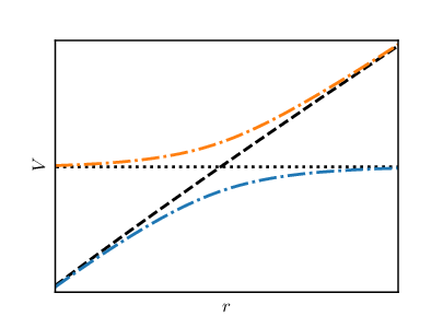
On the other hand, unquenched (with gluon and light-quark fields) lattice QCD calculations Bali et al. 2005; Bulava et al. 2019 have shown that due to string breaking the association of the light field ground state with a $Q\overline{Q}$ configuration holds only for small values of the relative $Q\overline{Q}$ distance $r\equiv\absolutevalue{\vb*{r}}$ . When increasing $r$ the $Q\overline{Q}$ configuration mixes significantly with meson-meson configurations. More in detail: below (above) an open-flavor meson-meson threshold the energy of a stationary state of the light fields changes with $r$ , from the one corresponding to the $Q\overline{Q}$ (meson-meson) configuration to the one of meson-meson ( $Q\overline{Q}$ ) configuration, avoiding in this manner the crossing of the static light field energies corresponding to pure $Q\overline{Q}$ and meson-meson configurations that would take place at the threshold mass in absence of string breaking. In Fig. 1 we have represented graphically this situation for $Q\overline{Q}$ and one meson-meson threshold (the representation for two meson-meson thresholds can be seen in Bali et al. 2005; Bulava et al. 2019).

Refer to caption — Figure 1: Pictorial representation of lattice static energies. Dashed line: ground state static light field energy in quenched lattice QCD. Dotted line: meson-meson threshold. Dash-dotted lines: ground and excited state static light field energies in unquenched lattice QCD, showing an avoided crossing.

II.2 Adiabatic expansion

Having solved the static problem for the light fields, the next step in the construction of the B-O approximation consists in reintroducing the $Q\overline{Q}$ motion. This is done by solving the bound state equation

\pqty{\frac{\vb*{p}^2}{2\mu_{Q\overline{Q}}} + H_\text{static}^\text{lf}(\vb*{r})-E}\ket{\psi}=0,

(7)

where $E$ denotes the mass of the bound state, making use of the so-called adiabatic expansion for $\ket{\psi}$ :

\ket{\psi}=\sum_{i}\int\differential{\bf\it r}^{\prime}\psi_{i}({\bf\it r}^{\prime})\ket{\vb*{r}^{\prime}}\ket{\zeta_{i}(\vb*{r}^{\prime})}

(8)

where $\ket{\vb*{r}^\prime}$ is a state indicating the $Q\overline{Q}$ relative position and we have temporarily omitted spin degrees of freedom for simplicity. The qualifier “adiabatic” refers to the fact that each term in the expansion depends only on a single value of ${\bf\it r}^{\prime}$ , what can be related to the physical situation where the light fields respond almost instantaneously to the motion of the quark and antiquark. However, as will be shown in what follows, this physical expansion is not mathematically convenient when configuration mixing takes place. Note that as the states $\ket{\zeta_{i}(\vb*{r}^\prime)}$ depend on ${\bf\it r}^{\prime}$ , so do the coefficients $\psi_{i}$ , one for each light field state.

Using (8) and multiplying on the left by $\bra{\vb*{r}}$ the bound state equation can be rewritten as

\sum_{i}\pqty{-\frac{\hbar^{2}}{2\mu_{Q\overline{Q}}}\laplacian+V_{i}(\vb*{r})-E}\psi_{i}({\bf\it r})\ket{\zeta_{i}(\vb*{r})}=0,

(9)

then multiplying on the left by $\bra{\zeta_{j}(\vb*{r})}$ yields

\sum_{i}\bqty{-\frac{\hbar^{2}}{2\mu_{Q\overline{Q}}}\mel{\zeta_{j}(\vb*{r})}{\laplacian\psi_{i}(\vb*{r})}{\zeta_{i}( \vb*{r})} + \pqty{V_{j}(\vb* {r})-E} \delta_{j i} \psi_{i}(\vb*{r})}=0.

(10)

The first term on the left hand side of (10) can be developed as

\matrixelement{\zeta_{j}(\vb*{r})}{\laplacian\psi_{i}(\vb*{r})}{\zeta_{i}(\vb*{r})}=\delta_{ji}\laplacian\psi_{i}({\bf\it r})+2{\bf\it\tau}_{ji}({\bf\it r})\dotproduct\gradient\psi_{i}({\bf\it r})+\tau_{ji}^{(2)}({\bf\it r})\psi_{i}({\bf\it r})

(11)

with

{\bf\it\tau}_{ji}({\bf\it r})\equiv\innerproduct{\zeta_{j}(\vb*{r})}{\grad\zeta_{i}(\vb*{r})}\mbox{\quad and\quad}\tau_{ji}^{(2)}({\bf\it r})\equiv\innerproduct{\zeta_{j}(\vb*{r})}{\laplacian\zeta_{i}(\vb*{r})}

(12)

being the so-called Non-Adiabatic Coupling Terms (NACTs) of the first and second order respectively.

Furthermore, using $\gradient\innerproduct{\zeta_{j}(\vb*{r})}{\zeta_{i}(\vb*{r})}=\gradient\delta_{ji}=0$ we have

{\bf\it\tau}_{ji}({\bf\it r})\equiv\innerproduct{\zeta_{j}(\vb*{r})}{\grad\zeta_{i}(\vb*{r})}=-\innerproduct{\grad\zeta_{j}(\vb*{r})}{\zeta_{i}(\vb*{r})}\equiv-{\bf\it\tau}_{ij}^{*}({\bf\it r}),

(13)

from which it follows

\innerproduct{\grad\zeta_{j}(\vb*{r})}{\grad\zeta_{i}(\vb*{r})}=\sum_{k}\innerproduct{\grad\zeta_{j}(\vb*{r})}{\zeta_{k}(\vb*{r})}\dotproduct\innerproduct{\zeta_{k}(\vb*{r})}{\grad\zeta_{i}(\vb*{r})}=\sum_{k}{\bf\it\tau}_{kj}^{*}({\bf\it r})\dotproduct{\bf\it\tau}_{ki}({\bf\it r})=-\sum_{k}{\bf\it\tau}_{jk}({\bf\it r})\dotproduct{\bf\it\tau}_{ki}({\bf\it r})\equiv-({\bf\it\tau}({\bf\it r})^{2})_{ji},

(14)

so that

(\gradient{\bf\it\tau}({\bf\it r}))_{ji}=\innerproduct{\zeta_{j}(\vb*{r})}{\laplacian\zeta_{i}(\vb*{r})}+\innerproduct{\grad\zeta_{j}(\vb*{r})}{\grad\zeta_{i}(\vb*{r})}=\tau_{ji}^{(2)}({\bf\it r})-({\bf\it\tau}({\bf\it r})^{2})_{ji}

(15)

and finally

\matrixelement{\zeta_{j}(\vb*{r})}{\laplacian\psi_{i}(\vb*{r})}{\zeta_{i}(\vb*{r})}=\delta_{ji}\laplacian\psi_{i}({\bf\it r})+2{\bf\it\tau}_{ji}({\bf\it r})\dotproduct\gradient\psi_{i}({\bf\it r})+((\divergence{\bf\it\tau}({\bf\it r}))_{ji}+({\bf\it\tau}({\bf\it r})^{2})_{ji})\psi_{i}({\bf\it r})\equiv((\gradient+{\bf\it\tau}({\bf\it r}))^{2})_{ji}\psi_{i}({\bf\it r}).

(16)

The bound state equation (10) then reads

\sum_{i}\bqty{ -\frac{\hbar^{2}}{2\mu_{Q\overline{Q}}}((\grad+\vb*{\tau}(\vb*{r}))^2)_{ji}+(V_{j}(\vb*{r})-E)\delta_{ji}}\psi_{i}({\bf\it r})=0.

(17)

This is a multichannel equation where $\psi_{i}({\bf\it r})$ stands for the $i$ -th component of the heavy-quark meson wave function, that is in general a mixing of $Q\overline{Q}$ and meson-meson components. Notice though that this is not the usual Schrödinger equation because of the presence of the NACTs ${\bf\it\tau}$ inside the kinetic energy operator. These terms introduce a coupling between the wave function components and reflect the non-trivial interaction between the $Q\overline{Q}$ motion and the light field states.

II.3 Single channel approximation

The last step in the construction of the B-O approximation consists in neglecting the NACTs inside the kinetic energy operator:

{\bf\it\tau}_{ji}({\bf\it r})=\innerproduct{\zeta_{j}(\vb*{r})}{\grad\zeta_{i}(\vb*{r})}\approx 0.

(18)

This is called the single channel approximation because the bound state equation (17) then factorizes in a set of decoupled single channel Schrödinger equations

\bqty{-\frac{\hbar^{2}}{2\mu_{Q\overline{Q}}}\laplacian+(V_{j}(\vb*{r})-E)}\psi_{j}({\bf\it r})=0

(19)

where $V_{j}({\bf\it r})$ , corresponding to the energy of the stationary $j$ -th state of the light fields in the presence of static $Q$ and $\overline{Q}$ sources, plays the role of an effective potential.

Eqs. (4), (8), (18) and (19) define the B-O approximation.

Notice that the single channel approximation can be deemed reasonable only up to $Q\overline{Q}$ distances for which the NACTs can be neglected, i.e. for distances where the $Q\overline{Q}$ and meson-meson configuration mixing associated with the light field eigenstates is negligible (for a specific calculation see Sec. IV.3). This makes the B-O approximation to be justified only for bound state energies far below the lowest open flavor meson-meson threshold. In particular, conventional heavy-quark meson masses, far below the lowest open flavor meson-meson threshold, can be described as the energy levels in the potential corresponding to the quenched ground state of the light fields, i.e. the Cornell potential.

III Diabatic approach

For energies close below or above an open flavor meson-meson threshold the mixing between the $Q\overline{Q}$ and meson-meson configurations gives rise to nonvanishing NACTs, so that the single channel approximation (18) cannot be maintained. Instead, one has to deal with the set of coupled equations (17), which is not practicable for two reasons:

i)

There is no yet direct lattice QCD calculation of the NACTs ${\bf\it\tau}$ .
ii)

When ${\bf\it\tau}\neq 0$ , the wave function components in the expansion (8) do not correspond to pure $Q\overline{Q}$ or meson-meson but rather to a mixing of both, the amount of mixing depending on ${\bf\it r}$ .

These drawbacks can be overcome through the use of the diabatic approach, where one expands the bound state $\ket{\psi}$ on a basis of light field eigenstates calculated at some fixed point ${\bf\it r}_{0}$ . As the $\Bqty{\ket{\zeta_i(\vb*{r})}}$ form a complete set for the light fields whatever the value of ${\bf\it r}$ , switching from a $\Bqty{\ket{\zeta_i(\vb*{r})}}$ to $\Bqty{\ket{\zeta_i(\vb*{r}_0)}}$ is equivalent to a ${\bf\it r}$ -dependent change of basis in the light degrees of freedom.

The diabatic expansion of the bound state reads

\ket{\psi}=\sum_{i}\int\differential{\vb*{r}^{\prime}}\widetilde{\psi}_{i}({\bf\it r}^{\prime},{\bf\it r}_{0})\ket{\vb*{r}^{\prime}}\ket{\zeta_{i}(\vb*{r}_{0})}

(20)

where the coefficients $\widetilde{\psi}_{i}$ , one coefficient for each light field state, are functions of ${\bf\it r}^{\prime}$ that depend parametrically on ${\bf\it r}_{0}$ .

A nice physical feature of this expansion is that the light field state $\ket{\zeta_i (\vb*{r}_0)}$ corresponding to each component $\widetilde{\psi}_{i}$ does not depend on the $Q\overline{Q}$ relative position ${\bf\it r}^{\prime}$ . This means that if one chooses the fixed point ${\bf\it r}_{0}$ far from the avoided crossing, then the wave function components correspond to either pure $Q\overline{Q}$ or meson-meson for any value of ${\bf\it r}^{\prime}$ . In other words, in the diabatic approach one expands the bound states in terms of the more intuitive Fock components (pure $Q\overline{Q}$ and pure meson-meson) instead of components which are a mixing of $Q\overline{Q}$ and meson-meson.

Substituting (20) in the bound state equation (7) and projecting on $\bra{\vb*{r}}$ yields

\sum_{i}\pqty{-\frac{\hbar^{2}}{2\mu_{Q\overline{Q}}}\laplacian+H_\text{static}^\text{lf}(\vb*{r})-E}\widetilde{\psi}_{i}({\bf\it r},{\bf\it r}_{0})\ket{\zeta_{i}(\vb*{r}_{0})}=0

(21)

where all the derivatives are taken with respect to ${\bf\it r}$ . If we now multiply on the left by $\bra{\zeta_{j}(\vb*{r}_{0})}$ , as $\gradient\ket{ \zeta_{i}(\vb*{r}_{0})}=0$ the equation reads

\sum_{i}\pqty{-\frac{\hbar^{2}}{2\mu_{Q\overline{Q}}}\delta_{ji} \laplacian+V_{ji}(\vb*{r},\vb*{r}_{0}) - E\delta_{ji}}\widetilde{\psi}_{i}({\bf\it r},{\bf\it r}_{0})=0

(22)

where

V_{ji}({\bf\it r},{\bf\it r}_{0})\equiv\matrixelement{\zeta_{j}(\vb*{r}_{0})}{H_\text{static}^\text{lf}(\vb*{r})}{\zeta_{i}(\vb*{r}_{0})}

(23)

is the so-called diabatic potential matrix.

The multichannel Schrödinger equation (22) together with (23) and (20) define the diabatic approach which is widely employed in molecular physics Baer 2006.

The complete equivalence between Eqs. (17) and (22) has been shown elsewhere Baer 2006 and is reproduced, for the sake of completeness, in Appendix A. In short, the troublesome NACTs in (17) that break the single channel approximation when configuration mixing is present (thus invalidating the B-O framework) are taken into account in (22) through the diabatic potential matrix. This is utterly convenient since, as we shall see in Sec. IV.2, the elements of this matrix are directly related to the static light field energy levels calculated in quenched and unquenched lattice QCD.

It is also easy to show that when the single channel approximation (18) holds the diabatic potential matrix (23) becomes a diagonal matrix containing the static light field energy levels calculated in quenched lattice QCD, and consequently Eq. (22) reproduces the set of single channel Schrödinger equations (19).

Therefore, the diabatic approach is a complete general framework appliable to conventional heavy-quark mesons lying far below the lowest open flavor meson-meson threshold as well as to unconventional ones lying close below or above that threshold.

IV Heavy-quark mesons in the diabatic framework

In order to apply the diabatic framework to the description of heavy-quark meson bound states we examine first the case of a single meson-meson threshold. Then we proceed to the generalization to an arbitrary number of thresholds.

IV.1 Spectroscopic equations

Let us consider one meson-meson threshold. Let us fix a value for ${\bf\it r}_{0}$ such that the ground state of the light fields is associated with the $Q\overline{Q}$ configuration and the first excited state with the meson-meson one. To make this more clear we relabel the diabatic light field states as

\ket{\zeta_0 (\vb*{r}_0)}\rightarrow\ket*{\zeta_{Q\overline{Q}}},\qquad\ket{\zeta_1 (\vb*{r}_0)}\rightarrow\ket*{\zeta_{M_1\overline{M}_2}},

(24)

and the diabatic wave function components as

\widetilde{\psi}_{0}({\bf\it r},{\bf\it r}_{0})\rightarrow\psi_{Q\overline{Q}}({\bf\it r}),\qquad\widetilde{\psi}_{1}({\bf\it r},{\bf\it r}_{0})\rightarrow\psi_{M_{1}\overline{M}_{2}}({\bf\it r}).

(25)

Accordingly, we rename the diabatic potential matrix components (23) as


$\displaystyle V_{00}({\bf\it r},{\bf\it r}_{0})\rightarrow V_{Q\overline{Q}}({\bf\it r})$	$\displaystyle=\matrixelement{\zeta_{Q\overline{Q}}}{H_\text{static}^\text{lf}(\vb{r})}{\zeta_{Q\overline{Q}}}$	(26a)
$\displaystyle V_{11}({\bf\it r},{\bf\it r}_{0})\rightarrow V_{M_{1}\overline{M}_{2}}({\bf\it r})$	$\displaystyle=\matrixelement{\zeta_{M_1\overline{M}_2}}{H_\text{static}^\text{lf}(\vb{r})}{\zeta_{M_1\overline{M}_2}}$	(26b)
$\displaystyle V_{01}({\bf\it r},{\bf\it r}_{0})\rightarrow V_{\text{mix}}({\bf\it r})$	$\displaystyle=\matrixelement{\zeta_{Q\overline{Q}}}{H_\text{static}^\text{lf}(\vb{r})}{\zeta_{M_1\overline{M}_2}}.$	(26c)

Let us realize that having associated each component of the wave function with pure $Q\overline{Q}$ or pure meson-meson, we can easily incorporate to the kinetic energy operator the fact that the reduced mass of the meson-meson component, $\mu_{M_{1}\overline{M}_{2}}$ , is different from $\mu_{Q\overline{Q}}$ . Hence, we shall use $-\frac{\hbar^{2}}{2\mu_{Q\overline{Q}}}\laplacian$ and $-\frac{\hbar^{2}}{2\mu_{M_{1}\overline{M}_{2}}}\laplacian$ for the kinetic energy operators of the $Q\overline{Q}$ and meson-meson components respectively. (Note that this improvement is possible only in the diabatic framework.)

Then, the bound state equations read


$\displaystyle\pqty{-\frac{\hbar^{2}}{2\mu_{Q\overline{Q}}}\laplacian+V_{Q\overline{Q}}(\vb*{r})-E}\psi_{Q\overline{Q}}({\bf\it r})+V_{\text{mix}}({\bf\it r})\psi_{M_{1}\overline{M}_{2}}({\bf\it r})$	$\displaystyle=0$	(27a)
$\displaystyle\pqty{-\frac{\hbar^{2}}{2\mu_{M_{1}\overline{M}_2}}\laplacian+ V_{M_1\overline{M}_2}(\vb*{r})-E}\psi_{M_{1}\overline{M}_{2}}({\bf\it r})+{V_{\text{mix}}({\bf\it r})}\psi_{Q\overline{Q}}({\bf\it r})$	$\displaystyle=0,$	(27b)

or in matrix notation

\pqty{\mathrm{K} + \mathrm{V}(\vb*{r})}\Psi({\bf\it r})=E\Psi({\bf\it r})

(28)

where $\mathrm{K}$ is the kinetic energy matrix

\mathrm{K}\equiv\pmqty{\lx@physics@matrix\endlx@physics@matrix},

(29)

$\mathrm{V}({\bf\it r})$ is the diabatic potential matrix

\mathrm{V}({\bf\it r})\equiv\pmqty{\lx@physics@matrix\endlx@physics@matrix},

(30)

and $\Psi({\bf\it r})$ is a column vector notation for the wave function:

\Psi({\bf\it r})\equiv\pmqty{\lx@physics@matrix\endlx@physics@matrix}.

(31)

In this notation the normalization of the wavefunciton reads

\int\differential{\vb*{r}}\Psi^{\dagger}({\bf\it r})\Psi({\bf\it r})=\mathcal{P}(Q\overline{Q})+\mathcal{P}(M_{1}\overline{M}_{2})=1

(32)

where we have defined the $Q\overline{Q}$ probability

\mathcal{P}(Q\overline{Q})\equiv\int\differential{\vb*{r}}\absolutevalue*{\psi_{Q\overline{Q}}(\vb*{r})}^{2}

(33)

and the meson-meson probability

\mathcal{P}(M_{1}\overline{M}_{2})\equiv\int\differential{\vb*{r}}\absolutevalue*{\psi_{M_{1}\overline{M}_2}(\vb*{r})}^{2}.

(34)

The multichannel Schrödinger equation (27), or equivalently (28), defines formally the diabatic approach for the description of the heavy-quark meson system.

IV.2 Mixing potential

To solve (27) we need to know the diabatic potential matrix Eq. (30). Regarding the diagonal element $V_{Q\overline{Q}}({\bf\it r})$ , we see from (26a) that it corresponds to the expectation value of the static energy operator in the light field state associated with a pure $Q\overline{Q}$ configuration. This can be identified with the ground state static energy calculated in quenched lattice QCD, see Fig. 1, given by the Cornell potential

V_{Q\overline{Q}}({\bf\it r})=V_{\text{C}}(r).

(35)

In the same way, from (26b) we identify the other diagonal term $V_{M_{1}\overline{M}_{2}}({\bf\it r})$ with the static energy associated with a pure meson-meson configuration, given by the threshold mass $T_{M_{1}\overline{M}_{2}}$ (the sum of the meson masses)

V_{M_{1}\overline{M}_{2}}({\bf\it r})=T_{M_{1}\overline{M}_{2}}\equiv m_{M_{1}}+m_{\overline{M}_{2}},

(36)

up to one pion exchange effects that we do not consider here.

As for the off-diagonal term, the mixing potential $V_{\text{mix}}({\bf\it r})$ , we can use the eigenvalues of the diabatic potential matrix to derive its form. As shown in Appendix A, these eigenvalues correspond to the static energy levels that are calculated in unquenched lattice QCD which have been pictorially represented in Fig. 1. More precisely, the eigenvalues of the diabatic potential matrix are the two solutions $V_{\pm}({\bf\it r})$ of the secular equation

\det{\mathrm{V}(\vb*{r}) - V_\pm(\vb*{r}) \mathbb{I}}=0

(37)

where $\mathbb{I}$ is the identity matrix. These solutions read

\begin{split}V_{\pm}({\bf\it r})=&\frac{V_{\text{C}}(r)+T_{M_{1}\overline{M}_{2}}}{2}\\ &\pm\sqrt{\pqty{\frac{V_\text{C}(r) - T_{M_1\overline{M}_2}}{2}}^{2}+V_{\text{mix}}({\bf\it r})^{2}},\end{split}

(38)

from which we obtain

\absolutevalue{V_\text{mix}(r)}=\frac{\sqrt{\pqty{V_+(r) - V_-(r)}^{2}-\pqty{V_\text{C}(r) - T_{M_1\overline{M}_2}}^{2}}}{2},

(39)

where we have dropped the vector notation for ${\bf\it r}$ as the energy levels calculated in lattice QCD depend only on the modulus $r=\absolutevalue{\vb*{r}}$ .

Eq. (39) tells us that a detailed calculation of the mixing potential $\absolutevalue{V_\text{mix}(r)}$ from ab initio lattice data on $V_{\pm}(r)$ is possible. As a matter of fact, an effective parametrization of $V_{\text{mix}}(r)$ from lattice data has been proposed Bulava et al. 2019; Bicudo et al. 2020. While we encourage more work along this direction, we resort to general arguments to get the shape of $\absolutevalue{V_\text{mix}(r)}$ . In this regard, the general form of the curves $V_{+}(r)$ and $V_{-}(r)$ near any threshold, reflecting the physical picture of the $Q\overline{Q}$ – meson-meson mixing, is expected to be similar as it happens to be the case when two thresholds are incorporated into the lattice calculation Bali et al. 2005; Bulava et al. 2019. Furthermore, the same form is expected for $Q=b$ and $Q=c$ since the underlying mixing mechanism (string breaking) is the same. Therefore, we shall proceed to a parametrization of $\absolutevalue{V_\text{mix}(r)}$ according to this general form, and we shall rely on phenomenology to fix the values of the parameters.

Let us begin by observing that unquenched lattice QCD results show that

\absolutevalue{V_+(r) - V_-(r)}\geq\absolutevalue{V_C (r) - T_{M_{1} \overline{M}_2}}

(40)

for every value $r$ , and that at the crossing radius $r_{\text{c}}^{M_{1}\overline{M}_{2}}$ , defined by

V_{\text{C}}\bigl(r_{\text{c}}^{M_{1}\overline{M}_{2}}\bigr)=T_{M_{1}\overline{M}_{2}},

(41)

$\absolutevalue{V_\text{mix}(r)}$ gets approximately its maximum value

\max_{r}\absolutevalue{V_\text{mix}(r)}\approx\absolutevalue{V_\text{mix}\bigl(r_\text{c}^{M_{1} \overline{M}_2}\bigr)}=\frac{\Delta}{2},

(42)

with $\Delta$ being the distance of the static energy levels at the crossing radius

\Delta\equiv\absolutevalue{V_+\bigl(r_\text{c}^{M_{1} \overline{M}_2}\bigr) - V_-\bigl(r_\text{c}^{M_{1} \overline{M}_2}\bigr)}.

(43)

On the other hand we have

V_{-}(r)\approx V_{\text{C}}(r)\mbox{\quad and\quad}V_{+}(r)\approx T_{M_{1}\overline{M}_{2}}

(44)

for $r\ll r_{\text{c}}^{M_{1}\overline{M}_{2}}$ , and

V_{-}(r)\approx T_{M_{1}\overline{M}_{2}}\mbox{\quad and\quad}V_{+}(r)\approx V_{\text{C}}(r)

(45)

for $r\gg r_{\text{c}}^{M_{1}\overline{M}_{2}}$ , so that

(V_{+}(r)-V_{-}(r))^{2}\approx(V_{\text{C}}(r)-T_{M_{1}\overline{M}_{2}})^{2}

(46)

far from the crossing radius $r_{\text{c}}^{M_{1}\overline{M}_{2}}$ . Consequently, from (39) we obtain that $V_{\text{mix}}(r)$ vanishes in both asymptotic limits:

\lim_{r\to 0}V_{\text{mix}}(r)=\lim_{r\to\infty}V_{\text{mix}}(r)=0.

(47)

To summarize, lattice QCD indicates that the mixing potential $\absolutevalue{V_\text{mix}(r)}$ approaches a maximum value of $\Delta/2$ at $r\approx r_{\text{c}}^{M_{1}\overline{M}_{2}}$ and vanishes asymptotically as the distance from the crossing radius increases. The simplest parametrization that takes into account these behaviors, thus providing a good fit to lattice QCD calculations of $V_{\pm}(r)$ , is a Gaussian shape:

\absolutevalue{V_\text{mix}(r)}=\frac{\Delta}{2}\exp{-\frac{\pqty{V_\text{C}(r)-T_{M_{1} \overline{M}_2}}^{2}}{2\Lambda^{2}}}

(48)

where $\Lambda$ is a parameter with dimensions of energy. To better understand the physical meaning of $\Lambda$ we write it in terms of the string tension $\sigma$ as

\Lambda\equiv\sigma\rho

(49)

where $\rho$ has now dimensions of length. Then at distances for which $V_{\text{C}}(r)\approx\sigma r+m_{Q}+m_{\overline{Q}}-\beta$ the mixing potential can be also written as

\absolutevalue{V_\text{mix}(r)}\approx\frac{\Delta}{2}\exp{-\frac{\bigl(r-r_\text{c}^{M_{1} \overline{M}_2}\bigr)^{2}}{2\rho^{2}}}

(48^′)

from which it is clear that $\rho$ , the width of the Gaussian curve, fixes a radial scale for the mixing.

IV.3 Configuration mixing

The knowledge of the diabatic potential matrix is quite equivalent to the knowledge of the $r$ -dependent change of basis matrix from $\Bqty{\ket{\zeta_0(r)}, \ket{\zeta_1(r)}}$ to $\Bqty{\ket{\zeta_0(r_0)},\ket{\zeta_1(r_0)}}$ . Let us name, according to our previous notation, $\ket*{\zeta_-(r)}\equiv\ket{\zeta_0(r)}$ and $\ket*{\zeta_+(r)}\equiv\ket{\zeta_1(r)}$ the ground and excited states of the light fields, with static energies $V_{-}(r)$ and $V_{+}(r)$ respectively. These are related to the $Q\overline{Q}$ and meson-meson states $\ket*{\zeta_{Q\overline{Q}}}\equiv\ket{\zeta_0(r_0)}$ and $\ket*{\zeta_{M_1\overline{M}_2}}\equiv\ket{\zeta_1(r_0)}$ via


$\displaystyle\ket{\zeta_-(r)}$	$\displaystyle=\cos(\theta(r))\ket{\zeta_{Q\overline{Q}}}+\sin(\theta(r))\ket{\zeta_{M_1\overline{M}_2}}$	(50a)
$\displaystyle\ket{\zeta_+(r)}$	$\displaystyle=\cos(\theta(r))\ket{\zeta_{M_1\overline{M}_2}}-\sin(\theta(r))\ket{\zeta_{Q\overline{Q}}}$	(50b)

where $\theta(r)$ is the mixing angle between the $Q\overline{Q}$ and meson-meson configurations.

As explained in Appendix A, the change of basis matrix connecting the two sets of states,

\pmqty{\lx@physics@matrix\endlx@physics@matrix}=\mathrm{A}^{\dagger}(r)\pmqty{\lx@physics@matrix\endlx@physics@matrix}

(51)

with

\mathrm{A}(r)\equiv\pmqty{\lx@physics@matrix\endlx@physics@matrix},

(52)

is also the matrix that diagonalizes the diabatic potential matrix. Therefore it is possible to extract the mixing angle $\theta$ from the matrix equation

\mathrm{A}(r)\mathrm{V}(r)\mathrm{A}^{\dagger}(r)=\text{diag}(V_{-}(r),V_{+}(r))

(53)

where $\text{diag}(V_{-}(r),V_{+}(r))$ is a diagonal 2 $\times$ 2 matrix containing the unquenched static light field energies. It is sufficient to take any off-diagonal element of Eq. (53) to obtain

V_{\text{mix}}(r)\cos(2\theta(r))=\frac{T_{M_{1}\overline{M}_{2}}-V_{\text{C}}(r)}{2}\sin(2\theta(r))

(54)

from which we get the mixing angle as

\theta(r)=\frac{1}{2}\arctan\biggl(\frac{2V_{\text{mix}}(r)}{T_{M_{1}\overline{M}_{2}}-V_{\text{C}}(r)}\biggr).

(55)

Furthermore, from this expression of the mixing angle and from Eqs. (50) we can also calculate the NACTs:


$\displaystyle{\bf\it\tau}_{00}(r)$	$\displaystyle={\bf\it\tau}_{11}(r)=0$	(56a)
$\displaystyle{\bf\it\tau}_{01}(r)$	$\displaystyle=-{\bf\it\tau}_{10}(r)$	(56b)

with

{\bf\it\tau}_{01}(r)\equiv\innerproduct{\zeta_-(r)}{\grad\zeta_+(r)}=(\mathrm{A}(r)\gradient\mathrm{A}^{\dagger}(r))_{01}=\hat{{\bf\it r}}\derivative{\theta}{r}.

(57)

Therefore the NACTs only vanish for values of $r$ where $\theta$ is constant. This happens for small (big) values of $r$ where $\theta$ is $0$ $(\pi/2)$ , corresponding to no mixing between the $Q\overline{Q}$ and meson-meson configurations in the light field eigenstates.

IV.4 General case

The multichannel Schrödinger equation (27) defines the heavy quark meson system when only one threshold is considered, but in general it may be necessary to incorporate several meson-meson thresholds. In such a case one has to extend the formalism, what is is more easily done in the matrix notation (28).

The generalization of the kinetic energy matrix is straightforward:

\mathrm{K}=\begin{pmatrix}-\frac{\hbar^{2}}{2\mu_{Q\overline{Q}}}\laplacian&&&\\ &-\frac{\hbar^{2}}{2\mu^{(1)}_{M\overline{M}}}\laplacian&&\\ &&\ddots&\\ &&&-\frac{\hbar^{2}}{2\mu^{(N)}_{M\overline{M}}}\laplacian\\ \end{pmatrix}

(58)

where $\mu_{M\overline{M}}^{(i)}$ with $i=1,\dots,N$ is the reduced mass of the $i$ -th meson-meson component, $N$ is the number of meson-meson thresholds, and matrix elements equal to zero are not displayed.

As for the extension of the diabatic potential matrix (30), the presence of interaction terms between different meson-meson components would make not practicable our procedure to extract the mixing potentials. Following what it is usually done in molecular physics Baer 2006, we neglect some interactions between components. Namely, in line with lattice QCD studies of string breaking Bulava et al. 2019, we assume that different meson-meson components do not interact with each other.

It seems reasonable to think that this is a good approximation when dealing with relatively narrow, well-separated thresholds. If so, we may consider the uncertainty of this approximation to be proportional to the ratio between the average of the threshold widths and the threshold mass difference. More precisely, for values of this ratio smaller than one we expect the threshold-threshold interaction to be negligible. According to this, we restrict our study to non-overlapping, narrow thresholds.

Then, the diabatic potential matrix with $N$ thresholds reads

\mathrm{V}(r)=\begin{pmatrix}V_{\text{C}}(r)&V_{\text{mix}}^{(1)}(r)&\ldots&V_{\text{mix}}^{(N)}(r)\\ {V_{\text{mix}}^{(1)}(r)}&T_{M\overline{M}}^{(1)}&&\\ \vdots&&\ddots&\\ {V_{\text{mix}}^{(N)}(r)}&&&T_{M\overline{M}}^{(N)}\\ \end{pmatrix}

(59)

where $V_{\text{C}}(r)$ stands for the Cornell potential, $T_{M\overline{M}}^{(i)}$ for the mass of the $i$ -th threshold and $V_{\text{mix}}^{(i)}(r)$ for the mixing potential between the $Q\overline{Q}$ and the $i$ -th meson-meson components.

In Fig. 2 we draw the eigenvalues of this matrix for $c\overline{c}$ and the first three open flavor meson-meson thresholds.

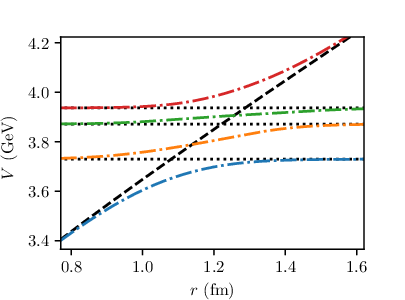
The diabatic potential matrix (59) can be regarded as a generalization of the two threshold model of string breaking introduced in Bulava et al. 2019, the two main differences being that in our study each dynamical quark flavor can introduce more than one threshold and that we have parametrized the coupling between quark-antiquark and meson-meson components with a Gaussian instead of a constant.

Let us add that even tough there is presumably an infinite number of possible meson-meson components, in practice one needs to consider only a limited subset of them when searching for bound states. As a matter of fact, a meson-meson component hardly plays any role in the composition of a bound state whose mass lies far below the corresponding threshold.

IV.5 Quantum numbers

Heavy-quark meson states are characterized by quantum numbers $I^{G}\pqty{J^{PC}}$ where $I$ , $G$ , $J$ , $P$ , $C$ stand for the isospin, G-parity, total angular momentum, parity, and charge conjugation quantum numbers respectively.

Let us focus on isoscalars $I=0$ heavy-quark mesons, for which $G=C$ . Since the diabatic potential matrix is spherically symmetric and spin-independent, the $Q\overline{Q}$ component of the wave function can be characterized by the relative orbital angular momentum quantum number $l_{Q\overline{Q}}$ , the total spin $s_{Q\overline{Q}}$ , the total angular momentum $J$ and its projection $m_{J}$ so that


$\displaystyle{\bf\it L}^{2}_{Q\overline{Q}}Y_{l_{Q\overline{Q}}}^{m_{l}}(\hat{{\bf\it r}})$	$\displaystyle=\hbar^{2}l_{Q\overline{Q}}(l_{Q\overline{Q}}+1)Y_{l_{Q\overline{Q}}}^{m_{l}}(\hat{{\bf\it r}})$	(60a)
$\displaystyle{\bf\it S}^{2}_{Q\overline{Q}}\xi_{s_{Q\overline{Q}}}^{m_{s}}$	$\displaystyle=\hbar^{2}s_{Q\overline{Q}}(s_{Q\overline{Q}}+1)\xi_{s_{Q\overline{Q}}}^{m_{s}}$	(60b)
$\displaystyle{\bf\it J}^{2}\bqty{Y_{l_{Q\overline{Q}}}(\vu*{r}) \xi_{s_{Q\overline{Q}}}}_{J}^{m_{J}}$	$\displaystyle=\hbar^{2}J(J+1)\bqty{Y_{l_{Q\overline{Q}}}(\vu*{r}) \xi_{s_{Q\overline{Q}}}}_{J}^{m_{J}}$	(60c)
$\displaystyle J_{z}\bqty{Y_{l_{Q\overline{Q}}}(\vu*{r}) \xi_{s_{Q\overline{Q}}}}_{J}^{m_{J}}$	$\displaystyle=\hbar\,m_{J}\bqty{Y_{l_{Q\overline{Q}}}(\vu*{r}) \xi_{s_{Q\overline{Q}}}}_{J}^{m_{J}}$	(60d)

where $Y_{l}^{m_{l}}(\hat{{\bf\it r}})$ is the spherical harmonic of degree $l$ , $\xi_{s}^{m_{s}}$ is the eigenstate of the total $Q\overline{Q}$ spin and $\bqty{Y_{l_{Q\overline{Q}}}(\vu*{r}) \xi_{s_{Q\overline{Q}}}}_{J}^{m_{J}}$ is a shorthand notation for the sum

\bqty{Y_{l_{Q\overline{Q}}} (\vu*{r}) \xi_{s_{Q\overline{Q}}}}_{J}^{m_{J}}\equiv\sum_{m_{l},m_{s}}C_{l_{Q\overline{Q}},s_{Q\overline{Q}},J}^{m_{l},m_{s},m_{J}}Y_{l_{Q\overline{Q}}}^{m_{l}}(\hat{{\bf\it r}})\xi_{s_{Q\overline{Q}}}^{m_{s}}

(61)

where $C_{l,s,J}^{m_{l},m_{s},m_{J}}$ is the Clebsch-Gordan coefficient. Given this set of quantum numbers, the $Q\overline{Q}$ component of the wave function can be factorized as

\psi_{Q\overline{Q}}({\bf\it r})=u^{(Q\overline{Q})}_{E,l_{Q\overline{Q}}}(r)\bqty{Y_{l_{Q\overline{Q}}}(\vu*{r}) \xi_{s_{Q\overline{Q}}}}_{J}^{m_{J}}

(62)

where $u^{(Q\overline{Q})}_{E,l_{Q\overline{Q}}}(r)$ is the $Q\overline{Q}$ radial wave function.

The same can be done for the meson-meson components of the wave function, considering the meson-meson relative orbital angular momentum $l_{M_{1}\overline{M}_{2}}$ and the sum of their spins $s_{M_{1}\overline{M}_{2}}$ . Therefore, with a straightforward extension of the above notation we write

\psi_{M_{1}\overline{M}_{2}}({\bf\it r})=u^{(M_{1}\overline{M}_{2})}_{E,l_{M_{1}\overline{M}_{2}}}(r)\bqty{Y_{l_{M_1\overline{M}_2}}(\vu*{r}) \xi_{s_{M_1\overline{M}_2}}}_{J}^{m_{J}}.

(63)

Note that for the spectroscopic state to have a definite value of $J$ , the $Q\overline{Q}$ and all the meson-meson components must have the same total angular momentum, hence the unified notation for $J$ .

A bound state made of $Q\overline{Q}$ and meson-meson has definite parity and $C$ -parity only if all the wave function components have the same parity under these transformations. This requirement translates into different conditions depending on whether the wave function component is associated with $Q\overline{Q}$ or meson-meson. For the $Q\overline{Q}$ component, $P$ and $C$ quantum numbers are given by

P=(-1)^{l_{Q\overline{Q}}+1}\mbox{\quad and\quad}C=(-1)^{l_{Q\overline{Q}}+s_{Q\overline{Q}}}.

(64)

On the other hand, for each meson-meson component one has

P=P_{M_{1}}P_{\overline{M}_{2}}(-1)^{l_{M_{1}\overline{M}_{2}}}

(65)

where $P_{M}$ is the parity of the meson. As for $C$ -parity, one has to consider two distinct cases: if $M_{1}=M_{2}$ the $C$ -parity of the meson-meson component is given by

C=(-1)^{l_{M_{1}\overline{M}_{2}}+s_{M_{1}\overline{M}_{2}}},

(66)

if otherwise $M_{1}\neq M_{2}$ one can build both positive and negative $C$ -parity states

C\ket*{M_1 \overline{M}_2}_{\pm}=\pm\ket*{M_1 \overline{M}_2}_{\pm}

(67)

taking the linear combinations

\ket*{M_1 \overline{M}_2}_{\pm}\equiv\frac{1}{\sqrt{2}}\pqty{\ket*{M_1 \overline{M_2}}_0 \pm\mathcal{C}_{M_1 \overline{M}_2} \ket*{M_2 \overline{M}_1}_0}

(68)

with $\ket*{M_1 \overline{M}_2}_{0}$ being the isospin singlet state obtained from the combination of the $M_{1}$ and $\overline{M}_{2}$ isomultiplets and

\mathcal{C}_{M_{1}\overline{M}_{2}}\equiv(-1)^{l_{M_{1}\overline{M}_{2}}+s_{M_{1}\overline{M}_{2}}+l_{M_{1}}+l_{\overline{M}_{2}}+s_{M_{1}}+s_{\overline{M}_{2}}+j_{M_{1}}+j_{\overline{M}_{2}}}

(69)

where $l_{M}$ is the internal orbital angular momentum of the meson, $s_{M}$ its internal spin and $j_{M}$ its total spin. The derivation of Eqs. (68) and (69) is detailed in Appendix B.

IV.6 Bound state solutions

Given a spherically-symmetric and spin-independent diabatic potential matrix, each $Q\overline{Q}$ configuration with a distinct value of $(l_{Q\overline{Q}},s_{Q\overline{Q}})$ can be treated as a channel per se, and the same can be said for each meson-meson configuration with a distinct value of $(l_{M_{1}\overline{M}_{2}},s_{M_{1}\overline{M}_{2}})$ . Then finding the spectrum of a given $J^{PC}$ family boils down to solving a multichannel, spherical Schrödinger equation involving only those channels with the corresponding $J^{PC}$ quantum numbers.

One should realize though that a complete numerical nonperturbative solution of the spectroscopic equations (28) is only possible for energies below the lowest $J^{PC}$ threshold. Above it the asymptotic behavior of its meson-meson component as a free wave, against the confined $Q\overline{Q}$ wave, prevents obtaining a physical solution. Nonetheless, an approximate physical solution for energies above threshold is still possible, under the assumption that the effect of an open threshold on the above-lying bound states can be treated perturbatively. More in detail, we proceed in the following way:

i)

We build the effective $J^{PC}$ diabatic potential matrix out of the Cornell $Q\overline{Q}$ potential, the threshold masses, and the $Q\overline{Q}$ – meson-meson mixing potentials.
ii)

We solve the spectroscopic equations for energies up to the lowest $J^{PC}$ threshold mass, and we analyze the $(n\,{{}^{2S+1}\!L}_{J})$ $Q\overline{Q}$ and meson-meson content of the bound states.
iii)

We build a new $J^{PC}$ diabatic potential matrix neglecting the $Q\overline{Q}$ coupling to the lowest (first) threshold. We solve it for energies in between the lowest and the second thresholds and discard as spurious any solution containing a $(n\,{{}^{2S+1}\!L}_{J})$ $Q\overline{Q}$ state entering in the bound states calculated in ii). The rationale underlying this step is that a given spectral state in between the lowest and the second thresholds containing such a $(n\,{{}^{2S+1}\!L}_{J})$ $Q\overline{Q}$ component would become, when the lowest threshold were incorporated, the bound state below threshold containing it found in ii).
iv)

We build a new $J^{PC}$ diabatic potential matrix by neglecting the coupling to the lowest threshold and to the second one. We solve it for energies in between the second and the third thresholds and discard as spurious any solution containing a $(n\,{{}^{2S+1}\!L}_{J})$ $Q\overline{Q}$ state entering in the bound states calculated in ii) and iii), and so on.
v)

We assume that corrections to the physical states thus obtained due to the coupling with open thresholds can be implemented perturbatively.

The formulation of an appropriate perturbative scheme for the calculation of these corrections, giving rise to mass shifts as well as to decay widths to open flavor meson-meson states, will be the subject of a forthcoming paper. On the other hand there are certainly more corrections to the spectrum that are not included in our treatment, in particular those due to spin interactions. Regarding the $Q\overline{Q}$ component, these effects can be incorporated by adding spin-dependent operators (e.g. spin-spin, spin-orbit, tensor) to the Cornell potential, what has proven to be very effective for a detailed description of the low-lying spectral states Godfrey and Isgur 1985. As for meson-meson components, the part of these corrections involving quark and antiquark within the same heavy-light meson are included through the meson masses, whereas the remaining ones can be implemented through the one pion exchange interaction between mesons.

Assuming that these additional energy contributions (fine and hyperfine splittings, one pion exchange corrections, mass shifts from coupling to open thresholds) can be taken into account using perturbation theory, we shall concentrate henceforth on the calculation of the “unperturbed” heavy-quark meson spectrum. The technical procedure followed to solve the spectroscopic equations is detailed in Appendices C and D.

V Charmonium-like mesons

The formalism we have developed in the previous sections can be tested in charmonium-like mesons (heavy mesons containing $c\overline{c}$ ) where, unlike in the bottomonium-like case, there are several well-established experimental candidates for unconventional isoscalar states, presumably containing significant meson-meson components. In particular, we center on isoscalar states with masses up to about $4.1$ GeV, for which the relevant thresholds have very small widths and do not overlap. A list of these thresholds is shown in Table 1.

$M_{1}\overline{M}_{2}$	$T_{M_{1}\overline{M}_{2}}$ (MeV)
$D\overline{D}$	$3730$
$D\overline{D}^{*}(2007)$	$3872$
$D_{s}^{+}D_{s}^{-}$	$3937$
$D^{}(2007)\overline{D}^{}(2007)$	$4014$
$D_{s}^{+}D_{s}^{*-}$	$4080$

Table 1: Low-lying open charm meson-meson thresholds

M_{1}\overline{M}_{2}

. Threshold masses

T_{M_{1}\overline{M}_{2}}

from the charmed and charmed strange meson masses quoted in Zyla et al. 2020.

The possible values of the meson-meson relative orbital angular momentum contributing to any given set of quantum numbers $J^{PC}$ are shown in Table 2. Note that we use the common notation $D_{(s)}$ to refer to charmed as well as to charmed strange mesons and the shorthand notation $D_{(s)}\overline{D}^{*}_{(s)}$ for the meson-meson $C$ -parity eigenstate defined by Eq. (68).

$J^{PC}$	$l_{D_{(s)}\overline{D}_{(s)}}$	$l_{D_{(s)}\overline{D}_{(s)}^{*}}$	$l_{D_{(s)}^{}\overline{D}_{(s)}^{}}$
$0^{++}$	$0$		0, 2
$1^{++}$		$0,\,2$	$2$
$2^{++}$	$2$	$2$	$0,\,2$
$1^{--}$	$1$	$1$	$1,\,3$

Table 2: Values of

l_{M_{1}\overline{M}_{2}}

corresponding to meson-meson configurations with definite values of

J^{PC}

. A missing entry means that the particular meson-meson configuration cannot form a state with the corresponding quantum numbers.

In order to calculate the heavy-quark meson bound states we have to fix the values of the parameters. For the Cornell potential (6) we use the standard values Eichten and Quigg 1994


	$\displaystyle\sigma$	$\displaystyle=925.6\text{\penalty\ MeV/fm},$	(70a)
	$\displaystyle\chi$	$\displaystyle=102.6\text{\penalty\ MeV\penalty\ fm},$	(70b)
	$\displaystyle m_{c}$	$\displaystyle=1840\text{\penalty\ MeV}$	(70c)
and we choose
	$\beta=855\text{\penalty\ MeV}$		(70d)

in order to fit the $2s$ center of gravity. Let us note that one could alternatively choose to fit the $1s$ or $1p$ centers of gravity, or to get a reasonable fit to the three of them. Our choice is based on the assumption that relativistic mass effects in the higher states, which are at least in part incorporated in $\beta$ , are expected to deviate less from those in the $2s$ states.

We should also mention that the value of the charm quark mass we use is completely consistent with the one needed to correctly describe $c\overline{c}$ electromagnetic decays within the Cornell potential model framework Bruschini and González 2020.

The low-lying spectrum from this Cornell potential for $J^{++}$ and $1^{--}$ isoscalar states is shown in Table 3.

$J^{PC}$	$nl$	$M_{c\overline{c}}$ (MeV)	$M_{\text{cog}}^{\text{Expt}}$ (MeV)
$1^{--}$	$1s$	$3082.5$	$3068.65\pm 0.13$
	$2s$	$3673.2$	$3674.0\pm 0.3$
	$1d$	$3795.8$
	$3s$	$4097.0$
$(0,1,2)^{++}$	$1p$	$3510.9$	$3525.30\pm 0.11$
$(0,1,2)^{++}$	$2p$	$3953.7$

Table 3: Calculated

J^{++}

and

1^{--}

charmonium masses,

M_{c\overline{c}}

, for spectroscopic

nl

states from the Cornell potential (6) with parameters (70). Experimental mass centroids from Zyla et al. 2020,

M_{\text{cog}}^{\text{Expt}}

, are listed for comparison.

For the lowest $J^{++}$ states it is worth to remark, apart from the good average mass description, the excellent fit to the mass of the lowest $1^{++}$ state, $\chi_{c_{1}}(1p)$ ( $3510.9$ MeV versus the experimental mass $3510.7$ MeV). However, an accurate fit of the lowest $(0,2)^{++}$ masses, in particular for $\chi_{c_{0}}(1p)$ , would require the incorporation of correction terms (e.g. spin-spin, spin-orbit, tensor) to the Cornell radial potential. As for the first excited $J^{++}$ states one could expect a similar situation (the $2s$ states lie in between the $1p$ and $2p$ ones $)$ in the absence of threshold effects that we analyse in what follows.

As for the parameters of the mixing potential (48), we have to rely on phenomenology since the only lattice information available is for $b\overline{b}$ . We fix them by requiring that our diabatic treatment fits the mass of some unconventional experimental state lying close below threshold. In particular, we can use the mass of $\chi_{c1}(3872)$ , a well-established experimental resonance lying just below the $D\overline{D}^{*}$ threshold, to infer the possible of values for $\Delta_{c\overline{c}}$ and $\rho_{c\overline{c}}$ .

As the crossing of the Cornell potential with the $D\overline{{D}}^{*}$ threshold takes place around $r_{\text{c}}^{D\overline{D}^{*}}=1.76$ fm, we conservatively vary $\rho_{c\overline{c}}$ from $0.1$ fm to $0.8$ fm, this last value corresponding to almost half of $r_{\text{c}}^{D\overline{D}^{*}}$ . Then, for every value of $\rho_{c\overline{c}}$ we get the minimal value of $\Delta_{c\overline{c}}$ to accurately fit the mass of $\chi_{c1}(3872)$ . The calculated values are listed in Table 4.

$\rho_{c\overline{c}}$ (fm)	$\Delta_{c\overline{c}}$ (MeV)
0.1	290
0.2	165
0.3	130
0.4	115
0.5	108
0.6	104
0.7	102
0.8	101

Table 4: Correlated values of the mixing potential parameters giving rise to a

0^{+}(1^{++})

bound state with a mass close below the

D\overline{D}^{*}

threshold.

It should be pointed out that large values of $\Delta_{c\overline{c}}$ would deform the shape of the avoided energy crossings as compared to the one calculated in lattice for $b\overline{b}$ , against our $b\overline{b}$ – $c\overline{c}$ universality arguments for the shape of the mixing potential. On the other hand, large values of $\rho_{c\overline{c}}$ would make the mixing angle between the $c\overline{c}$ and a single $M_{1}\overline{M}_{2}$ threshold, calculated from Eq. (55), to have an asymptotic behavior in conflict with the one observed in the lattice under the natural assumption that this behavior is similar for $b\overline{b}$ and $c\overline{c}$ . More precisely, unquenched lattice QCD calculations of the mixing angle Bali et al. 2005 show that $\theta$ approaches $\pi/2$ quite rapidly for $r>r_{\text{c}}^{M_{1}\overline{M}_{2}}$ , thus ruling out a large radial scale for the mixing. Henceforth we use

	$\rho_{c\overline{c}}=0.3\text{ fm}$	(71a)
for this value gives the most accurate asymptotic behavior of the mixing angle, see Fig. 3, and consequently
	$\Delta_{c\overline{c}}=130\text{\penalty\ MeV}.$	(71b)

The resulting mixing potential is drawn in Fig. 4 for $M_{1}\overline{M}_{2}=D\overline{D}^{*}$ . For any other threshold the only difference comes from the substitution of the threshold mass.

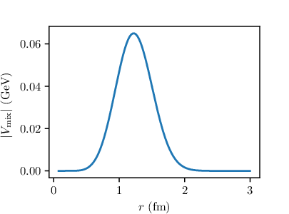
Notice that we have drawn $\absolutevalue{V_\text{mix}(r)}$ with no sign prescription for $V_{\text{mix}}(r)$ . This sign can be reabsorbed as a relative phase between the charmonium and meson-meson components. For the calculations in this paper a positive sign has been taken. We have checked that for the observables considered in this article the same results are obtained with a negative sign. It should be realized though that this could not be the case for other observables.

The calculated spectrum of $J^{++}$ states, containing one $c\overline{c}$ state with $l_{c\overline{c}}=1$ ( $1p$ or $2p$ ), is shown in Table 5.

$J^{PC}$	Mass (MeV)	$c\overline{c}$	$D\overline{D}^{*}$	$D_{s}\overline{D}_{s}$	$D^{}\overline{D}^{}$
$1^{++}$	3510.0	$100\%$
$1^{++}$	3871.7	$1\%$	$99\%$
$0^{++}$	3509.1	$100\%$
$0^{++}$	3920.4	$59\%$		$37\%$	$4\%$
$2^{++}$	3509.6	$100\%$
$2^{++}$	3933.5	$86\%$		$7\%$	$7\%$

Table 5: Calculated masses,

c\overline{c}

and meson-meson probabilities for

J^{++}

charmonium-like states. A missing entry means that the corresponding component gives negligible (i.e. inferior to

1\%

) or no contribution to the state.

It is illustrative to compare these results with the $c\overline{c}$ masses in Table 3 obtained with the Cornell potential. A glance at these tables makes clear that the presence of the thresholds gives rise to attraction in the sense that the resulting masses are reduced with respect the corresponding Cornell $c\overline{c}$ masses. For the lowest-lying $0^{+}(J^{++})$ states ( $J=0,1,2$ ) there is a very small mass difference indicating an almost negligible attraction for these states. This is understood for the thresholds are far above in energy ( $\geq 200$ MeV) so that no significant mixing occurs (less than $1\%$ meson-meson probability).

The situation is completely altered for the first excited $0^{+}(J^{++})$ states. Thus, the fitting of the first excited $1^{++}$ resonance, $\chi_{c_{1}}(3872)$ with a measured mass of $3871.69\pm 0.17$ MeV, requiring a mass reduction of $81$ MeV with respect to the Cornell $c\overline{c}$ mass, implies a very strong mixing, $99\%$ of $D\overline{D}^{*}$ component, whereas for the $0^{++}$ and $2^{++}$ states the predicted mixing is about $40\%$ (mainly from $D_{s}\overline{D}_{s})$ and $15\%$ (shared by $D_{s}\overline{D}_{s}$ and $D^{*}\overline{D}^{*})$ respectively, with corresponding mass reductions of $33$ MeV and $20$ MeV.

It is amazing that these $(0,2)^{++}$ mass predictions are in complete agreement with data regarding their positions with respect to the $D_{s}\overline{D}_{s}\$ threshold, both below it. Moreover, their calculated numerical values are pretty close to the measured ones. So, the calculated $2^{++}$ mass, $3933.5$ MeV, is very close to that of the experimental resonance $\chi_{c_{2}}(3930)$ : $3927.2\pm 2.6$ MeV. And the $0^{++}$ calculated mass, $3920.4$ MeV, is consistent with the ones of the experimental candidates: $\chi_{c_{0}}(3860)$ , with a measured mass of $3862_{-32-13}^{+26+40}$ MeV, and $X(3915)$ with a measured mass of $3918.4\pm 1.9$ MeV, although in this last case the assignment to a $2^{++}$ state cannot be completely ruled out, see Zyla et al. 2020 and references therein. This suggests that further mass corrections for these sates as the ones due to spin-dependent terms in the $c\overline{c}$ potential, or to one pion exchange in the meson-meson potential, or those taking into account the effect of the lower threshold $D\overline{D}$ , or the deviations from the assumption of the same values of the mixing potential parameters for all the thresholds, are either small and might be implemented perturbatively, or have been partially taken into account through the effectiveness of the parameters of the mixing potential.

It should also be emphasized that our nonperturbative formalism provides us with the meson wave functions in terms of their $c\overline{c}$ and meson-meson components.

For $\chi_{c_{1}}(3872)$ the radial $c\overline{c}$ and $D\overline{D}^{*}$ ( $l_{D\overline{D}^{*}}=0,2$ ) wave function components are plotted in Fig. 5.

A look at this figure makes clear the prevalence of the $D\overline{D}^{*}$ channel with $l_{D\overline{D}^{*}}=0$ for distances beyond $2$ fm. As the estimated Cornell rms radius for $D$ is about $0.54$ fm we may conclude that $\chi_{c_{1}}(3872)$ , with a calculated rms radius of $26.17$ fm is at large distances a loose hadromolecular state. At short distances, though, the $(2\,{{}^{3}\!p}_{1})$ $c\overline{c}$ component, with a rms radius of $1.01$ fm plays a role at least as prominent as the $D\overline{D}^{*}$ one, see Fig. 5. These features are quite in line with the indications from phenomenology requiring a $c\overline{c}$ component to give proper account of short distance properties.

For the calculated $0^{++}$ state the radial wave function is drawn in Fig. 6.

As can be checked, the wave function with a rms radius of $1.26$ fm is made mainly of $c\overline{c}$ and $D_{s}\overline{D}_{s}$ with a $59\%$ and $37\%$ probability respectively. This indicates a dominant $D\overline{D}$ strong decay mode from $c\overline{c}$ as it is experimentally the case for $\chi_{c_{0}}(3860)$ . On the other hand, a $J/\psi\,\omega$ decay mode may get a significant contribution from $D_{s}\overline{D}_{s}$ since it is OZI allowed through the small $s\overline{s}$ content of $\omega$ . This could cause this mode to be also a dominant one as it is experimentally the case for $X(3915)$ . Hence, it could be that $\chi_{c_{0}}(3860)$ and $X(3915)$ are just the same resonance observed through two different decay modes.

As for the calculated $2^{++}$ state, the wave function, with a rms radius of $1.06$ fm, is plotted in Fig. 7. It is mostly that of the $c\overline{c}$ component. This is in accord with a very dominant $D\overline{D}$ strong decay mode as it is experimentally the case for $\chi_{c_{2}}(3930)$ .

Certainly these qualitative arguments on the dominant strong decay modes should be supported by trustable and predictive quantitative calculations. As mentioned before, the development of a consistent formalism for the calculation of the decay widths to open flavor meson-meson states, which is out of the scope of this article, is in progress. One should keep in mind though that the dearth of current detailed quantitative decay data for comparison will be a serious drawback to test it. We strongly encourage experimental efforts along this line.

Regarding electromagnetic radiative transitions, although important progress for the accurate calculation of decays from the $c\overline{c}$ component has been reported Bruschini and González 2020, a reliable and consistent calculation incorporating the meson-meson contribution as well is lacking. We encourage a theoretical effort along this line.

One can do better, as we show next, for leptonic decays from the low-lying $1^{--}$ states since the decay widths depend on the wave function at the origin and the contribution from meson-meson components is suppressed as they are not in $s$ -wave, see Table 2.

The calculated $1^{--}$ spectrum of states is listed in Table 6.

$J^{PC}$	Mass (MeV)	$c\overline{c}$	$D\overline{D}$	$D\overline{D}^{*}$	$D_{s}\overline{D}_{s}$	$D_{s}\overline{D}_{s}^{*}$
$1^{--}$	3082.4	$100\%$
	3664.2	$95\%$	$4\%$	$1\%$
	3790.2	$97\%$		$2\%$	$1\%$
	4071.0	$64\%$				$36\%$

Table 6: Calculated masses,

c\overline{c}

and meson-meson probabilities for

1^{--}

charmonium-like states. A missing entry means that the corresponding component gives negligible (i.e. inferior to

1\%

) or no contribution to the state.

Again, a comparison with the $c\overline{c}$ masses in Table 3 makes clear that the presence of the thresholds gives rise to attraction. As it was the case for $J^{++}$ , the lowest state, lying far below the lowest threshold, has no mixing at all being the $1s$ $c\overline{c}$ state. A pretty small mixing is present for the next two higher states that can be mostly assigned to the $2s$ $(95\%)$ and $1d$ $(97\%)$ $c\overline{c}$ states respectively. It is worth to mention that for the $1d$ state with a Cornell $c\overline{c}$ mass of $3795.8$ MeV, the $D\overline{D}$ threshold lying $66$ MeV below does not produce enough attraction to bring the state below threshold.

The first state with a significant mixing, $36\%$ of $D_{s}\overline{D}_{s}^{*}$ , is predicted at $4071$ MeV and contains a $60\%$ of $3s$ $c\overline{c}$ and a $4\%$ of $2d$ $c\overline{c}$ as well. Its wave function is drawn in Fig. 8.

In this case the vicinity of the $D_{s}\overline{D}_{s}^{*}$ threshold at $4080$ MeV to the $3s$ $c\overline{c}$ Cornell mass at $4097$ MeV produces sufficient attraction to bring the state below threshold, in agreement with data under its assignment to the $\psi(4040)$ resonance with a measured mass of $4039\pm 1$ MeV. Furthermore the expected dominant decay modes, ( $D\overline{D},D\overline{D}^{*},D_{s}\overline{D}_{s},D^{*}\overline{D}^{*}$ ) from $c\overline{c}$ , and $D_{s}\overline{D}_{s}\,\gamma$ from $D_{s}\overline{D}_{s}^{*}$ , are in perfect accord with the ones observed from $e^{+}e^{-}\rightarrow\text{hadrons}$ .

As for the well-measured leptonic width

\left(\Gamma\left(\psi(4040)\rightarrow e^{+}e^{-}\right)\right)_{\text{Expt}}=0.86\pm 0.07\text{\penalty\ KeV},

(72)

we can trustfully predict the ratios

	$\frac{\Gamma_{\psi(4040)\rightarrow e^{+}e^{-}}^{\text{Theor}}}{\Gamma_{\psi(1s)\rightarrow e^{+}e^{-}}^{\text{Theor}}}=\frac{\absolutevalue{R_{\psi(4040)}(0)}^{2}}{\absolutevalue{R_{\psi(1s)}(0)}^{2}}\frac{M_{\psi(1s)}^{2}}{M_{\psi(4040)}^{2}}\\ \approx 0.18$	(73a)
and
	$\frac{\Gamma_{\psi(4040)\rightarrow e^{+}e^{-}}^{\text{Theor}}}{\Gamma_{\psi(2s)\rightarrow e^{+}e^{-}}^{\text{Theor}}}=\frac{\absolutevalue{R_{\psi(4040)}(0)}^{2}}{\absolutevalue{R_{\psi(2s)}(0)}^{2}}\frac{M_{\psi(2s)}^{2}}{M_{\psi(4040)}^{2}}\\ \approx 0.43$	(73b)

to be compared to

	$\frac{\Gamma_{\psi(4040)\rightarrow e^{+}e^{-}}^{\text{Expt}}}{\Gamma_{\psi(1s)\rightarrow e^{+}e^{-}}^{\text{Expt}}}=0.15\pm 0.03$	(74a)
and
	$\frac{\Gamma_{\psi(4040)\rightarrow e^{+}e^{-}}^{\text{Expt}}}{\Gamma_{\psi(2s)\rightarrow e^{+}e^{-}}^{\text{Expt}}}=0.37\pm 0.07.$	(74b)

Hence, our results agree with data within the experimental intervals. The reason for this agreement has to do with the reduced probability of the $3s$ $c\overline{c}$ component, $60\%$ , induced by the mixing with the $D_{s}\overline{D}_{s}^{*}$ threshold. This mixing is also responsible for the $4\%$ of $2d$ $c\overline{c}$ component. This small (big) $2d$ ( $3s$ ) probability could be increased (decreased) if a tensor interaction were incorporated as a correction term to the Cornell potential. Maybe the bias we observe in our results, both agreeing with the maximum allowed experimental values, is an indication in this sense. In any case a modest additional probability reduction of the $3s$ $c\overline{c}$ component should be expected.

It is worth to mention that the explanation of the leptonic width for $\psi(4040)$ has been linked in the literature to that of $\psi(4160)$ through a very significant $s$ - $d$ mixing Badalian et al. 2009. Our results do not support this idea. Instead the $D_{s}\overline{D}_{s}^{*}$ – $c\overline{c}(3s)$ mixing appears to be the main physical mechanism underlying the $\psi(4040)$ decay to $e^{+}e^{-}$ .

Unfortunately, at the current stage of our diabatic development we cannot properly evaluate $\psi(4160)$ , the main reason being that the dominant Cornell $2d$ $c\overline{c}$ state lies only $100$ MeV below the first $s$ -wave $1^{--}$ threshold, $D\overline{D}_{1}$ , which is composed of two overlapping thresholds, $D\overline{D}_{1}(2420)$ and $D\overline{D}_{1}(2430)$ , the last one with a large width. Quite presumably this double threshold gives a significant contribution by itself to the leptonic width of $\psi(4160)$ .

This current limitation applies as well to the description of unconventional states with masses above $4.1$ GeV such as $\psi(4260)$ lying close below the $D\overline{D}_{1}$ double threshold, or $\psi(4360)$ and $\psi(4415)$ lying close below a multiple threshold at $4429$ MeV. The same limitation applies for $J^{++}$ states. Work along this line is in progress.

VI Summary and conclusions

A general formalism for a unified description of conventional and unconventional heavy-quark meson states has been developed and successfully applied to isoscalar $J^{++}$ and $1^{--}$ charmonium-like states with masses below $4.1$ GeV.

The formalism adapts the diabatic approach, widely used in molecular physics to tackle the configuration mixing problem, to the study of heavy-quark meson states involving quark-antiquark as well as meson-meson components. A great advantage of using this approach, against the Born-Oppenheimer (B-O) approximation commonly used for heavy-quark mesons, is that the bound states are expanded in terms of $Q\overline{Q}$ and meson-meson configurations instead of the mixed configurations that correspond to the ground and excited states of the light fields. Then instead of being forced to use a single channel approximation to solve the bound state problem as in B-O, what in practice is equivalent to neglect the configuration mixing, one can write a treatable multichannel Schrödinger equation where the interaction between configurations is incorporated through a diabatic potential matrix. Moreover, the diagonal and off-diagonal elements of this potential matrix can be directly related to the static energies obtained from ab initio quenched (only $Q\overline{Q}$ or meson-meson configuration) and unquenched ( $Q\overline{Q}$ and meson-meson configurations) lattice calculations. This connection defines the diabatic approach in QCD.

It is worth to emphasize that this approach goes also beyond the incorporation of hadron loop corrections to the B-O scheme that have been used sometimes in the literature to deal with unconventional charmonium-like mesons. Indeed, the diabatic bound state wave functions, given in terms of quark-antiquark and meson-meson components, allow for a complete nonperturbative evaluation of observable properties.

This theoretical framework has been tested in the charmonium-like meson sector where there is compelling evidence of the existence of mixed-configuration states, in particular the very well-established $0^{+}(1^{++})$ resonance $\chi_{c_{1}}(3872)$ that we use to fix our parametrization of the mixing potential.

Although a complete (at all energies) spectral description would require additional theoretical refinements, as for example the incorporation of threshold widths, the results obtained for states with mass below $4.1$ GeV, for which the significant thresholds are very narrow, are encouraging. All the mass values are well reproduced and their locations with respect to the thresholds correctly predicted making clear the $c\overline{c}$ – threshold attraction. This points out to the diabatic approach as an appropriate framework for a unified and complete nonperturbative description of heavy-quark meson states.

Acknowledgements.

This work has been supported by MINECO of Spain and EU Feder Grant No. FPA2016-77177-C2-1-P, by SEV-2014-0398, by EU Horizon 2020 Grant No. 824093 (STRONG-2020) and by PID2019-105439GB-C21. R. B. acknowledges a FPI fellowship from MICIU of Spain under Grant No. BES-2017-079860.

Appendix A Adiabatic-to-diabatic transformation

As the light field eigenstates $\ket{\zeta_{i}(\vb*{r})}$ form a complete orthonormal set whatever the value of ${\bf\it r}$ , we can express (we use hereby Einstein notation so that a sum over repeated indices is understood)

\ket{\zeta_{j}(\vb*{r}_0)}=\ket{\zeta_{i}(\vb*{r})}A_{ij}({\bf\it r},{\bf\it r}_{0})

(75)

where $A_{ij}({\bf\it r},{\bf\it r}_{0})$ is a change of basis unitary matrix defined formally by

A_{ij}({\bf\it r},{\bf\it r}_{0})\equiv\innerproduct{\zeta_{i}(\vb*{r})}{\zeta_{j}(\vb*{r}_0)}.

(76)

This matrix, which is a function of the coordinate ${\bf\it r}$ and depends parametrically on the fixed point ${\bf\it r}_{0}$ , is referred to in this context as the Adiabatic-to-Diabatic Transformation matrix (ADT matrix). Let us examine the conditions to be satisfied by the ADT matrix for the adiabatic and diabatic expansions to be equivalent Baer 2006.

Let us begin by inserting (75) in the diabatic expansion (20) and comparing with (8). We thus see that the ADT matrix transforms the diabatic wave function in the adiabatic one:

\psi_{i}({\bf\it r})=A_{ij}({\bf\it r},{\bf\it r}_{0})\widetilde{\psi}_{j}({\bf\it r},{\bf\it r}_{0}).

(77)

If we now plug (77) into Eq. (17) and multiply on the left by $\mathrm{A}^{\dagger}$ we obtain

\bqty{-\frac{\hbar^2}{2\mu_{Q\overline{Q}}}A^\dagger_{i k}((\grad+ \vb*{\tau})^2)_{k l} A_{l j} + (A^\dagger_{i k}V_k A_{k j} - \delta_{i j} E)}\widetilde{\psi}_{j}=0,

(78)

where we have momentarily dropped the arguments ${\bf\it r}$ and ${\bf\it r}_{0}$ to simplify the notation. Using

\begin{split}((\gradient+{\bf\it\tau})^{2})_{kl}A_{lj}\widetilde{\psi}_{j}=&(\delta_{km}\gradient+{\bf\it\tau}_{km})\dotproduct(\delta_{ml}\gradient+{\bf\it\tau}_{ml})A_{lj}\widetilde{\psi}_{j}\\ =&(\delta_{km}\gradient+{\bf\it\tau}_{km})\dotproduct(A_{mj}\gradient+(\gradient A)_{mj}+{\bf\it\tau}_{ml}A_{lj})\widetilde{\psi}_{j}\\ =&[A_{kj}\laplacian+2(\gradient A)_{kj}\dotproduct\gradient+(\laplacian A)_{kj}+(\divergence{\bf\it\tau})_{kl}A_{lj}+2{\bf\it\tau}_{kl}\dotproduct(\gradient A)_{lj}+2{\bf\it\tau}_{kl}\dotproduct A_{lj}\gradient+({\bf\it\tau}^{2})_{kl}A_{lj}]\widetilde{\psi}_{j}\\ =&[A_{kj}\laplacian+((\gradient A)_{kj}+{\bf\it\tau}_{kl}A_{lj})\dotproduct\gradient+(\delta_{kl}\gradient+{\bf\it\tau}_{kl})\dotproduct((\gradient A)_{lj}+{\bf\it\tau}_{lm}A_{mj})]\widetilde{\psi}_{j},\end{split}

(79)

we can expand the kinetic term as

A^{\dagger}_{ik}((\gradient+{\bf\it\tau})^{2})_{kl}A_{lj}=\delta_{ij}\laplacian+A^{\dagger}_{ik}((\gradient A)_{kj}+{\bf\it\tau}_{kl}A_{lj})\dotproduct\gradient+(A^{\dagger}_{il}\gradient+A^{\dagger}_{ik}{\bf\it\tau}_{kl})\dotproduct((\gradient A)_{lj}+{\bf\it\tau}_{lm}A_{mj}).

(80)

Therefore, as in the diabatic representation the kinetic term is diagonal, the ADT matrix must satisfy the first order differential equation

\gradient A_{ij}({\bf\it r},{\bf\it r}_{0})+{\bf\it\tau}_{ik}({\bf\it r})A_{kj}({\bf\it r},{\bf\it r}_{0})=0,

(81)

where we have restored the arguments ${\bf\it r}$ and ${\bf\it r}_{0}$ .

Eq. (81), together with the boundary condition $A_{ij}({\bf\it r}_{0},{\bf\it r}_{0})=\delta_{ij}$ , determines uniquely the ADT matrix for every point in configuration space, if the NACTs are well-behaved. If otherwise the NACTs present singularities, the ADT matrix may be multi-valued Baer 2006. We will not examine this latter possibility here.

Substituting (80)-(81), Eq. (78) becomes

\bqty{-\frac{\hbar^2}{2\mu_{Q\overline{Q}}}\delta_{i j} \laplacian+ (A^\dagger_{i k}(\vb*{r}, \vb*{r}_0) V_k(\vb*{r}) A_{k j}(\vb*{r}, \vb*{r}_0) - \delta_{i j} E)}\widetilde{\psi}_{j}({\bf\it r},{\bf\it r}_{0})=0,

(82)

which can be recognized as the diabatic Schrödinger equation (22) by requiring

A^{\dagger}_{ik}({\bf\it r},{\bf\it r}_{0})V_{k}({\bf\it r})A_{kj}({\bf\it r},{\bf\it r}_{0})=V_{ij}({\bf\it r},{\bf\it r}_{0}).

(83)

This requirement tells us that the ADT matrix diagonalizes the diabatic potential matrix, and that the eigenvalues of the diabatic potential matrix are then the unquenched static energies $V_{i}({\bf\it r})$ .

It is thus proved that the diabatic and adiabatic expansions are completely equivalent, so that the NACTs together with the unquenched static energies carry the same amount of physical information as the diabatic potential matrix.

Appendix B $C$ -parity of meson-meson states

Although heavy-light mesons do not have definite $C$ -parity nor $G$ -parity, meson-meson configurations with $I=0$ can be rearranged in combinations with definite $C$ -parity. To build these combinations let us start by observing the action of $C$ -parity on some heavy-light meson state $M$ made of a light quark $q$ and a heavy antiquark $\overline{Q}$ :

C\ket{M}=(-1)^{l_{M}+s_{M}}\ket{\overline{M}}

(84)

where $l_{M}$ and $s_{M}$ , the internal orbital angular momentum and internal spin of the meson, are given in terms of the $q\overline{Q}$ relative orbital angular momentum and total spin respectively. Next we consider the action of $C$ -parity on the isospin singlet state formed by a $q\overline{Q}$ meson $M_{1}$ and a $Q\overline{q}$ meson $\overline{M}_{2}$

C\ket*{M_1 \overline{M}_2}_{0}=(-1)^{l_{M_{1}}+s_{M_{2}}+l_{\overline{M}_{2}}+s_{\overline{M}_{2}}}\ket*{\overline{M}_1 M_2}_{0}.

(85)

We now exchange the positions and spin labels of the mesons in $\ket*{\overline{M}_1 M_2}_{0}$ , thus obtaining an additional sign:

\ket*{\overline{M}_1 M_2}_{0}=(-1)^{l_{M_{1}\overline{M}_{2}}+s_{M_{1}\overline{M}_{2}}+j_{M_{1}}+j_{\overline{M}_{2}}}\ket*{M_2 \overline{M}_1}_{0}

(86)

where $j_{M}$ is the total spin of the meson given by the sum of the meson internal orbital angular momentum and spin. Note that the factor $(-1)^{l_{M_{1}\overline{M}_{2}}}$ comes from the exchange of the positions and the factor $(-1)^{s_{M_{1}\overline{M}_{2}}+j_{M_{1}}+j_{\overline{M}_{2}}}$ comes from the exchange of the spin labels. Then substituting (86) in (85) we obtain

C\ket*{M_1 \overline{M}_2}_{0}=\mathcal{C}_{M_{1}\overline{M_{2}}}\ket*{M_2 \overline{M}_1}_{0}

(87)

where

\mathcal{C}_{M_{1}\overline{M}_{2}}\equiv(-1)^{l_{M_{1}\overline{M}_{2}}+s_{M_{1}\overline{M}_{2}}+l_{M_{1}}+l_{\overline{M}_{2}}+s_{M_{1}}+s_{\overline{M}_{2}}+j_{M_{1}}+j_{\overline{M}_{2}}}.

(88)

From Eq. (87) it is then straightforward to prove that the states

\ket*{M_1 \overline{M}_2}_{\pm}\equiv\frac{1}{\sqrt{2}}\pqty{\ket*{M_1 \overline{M_2}}_0 \pm\mathcal{C}_{M_1 \overline{M}_2} \ket*{M_2 \overline{M}_1}_0}

(89)

have definite $C$ -parity:

\begin{split}C\ket*{M_1\overline{M}_2}_{\pm}&=\frac{1}{\sqrt{2}}\pqty{C \ket*{M_1\overline{M}_2}_0 \pm\mathcal{C}_{M_1 \overline{M_2}} C \ket*{M_2\overline{M}_1}_0}\\ &=\frac{1}{\sqrt{2}}\pqty{\mathcal{C}_{M_1 \overline{M_2}} \ket*{M_2\overline{M}_1}_0 \pm\ket*{M_1\overline{M}_2}_0}\\ &=\pm\frac{1}{\sqrt{2}}\pqty{\ket*{M_1\overline{M}_2}_0 \pm\mathcal{C}_{M_1 \overline{M_2}} \ket*{M_2\overline{M}_1}_0}\\ &\equiv\pm\ket*{M_1\overline{M}_2}_{\pm},\end{split}

(90)

where we have used the fact that $\mathcal{C}_{M_{1}\overline{M_{2}}}^{2}=(\pm)^{2}=1$ .

Appendix C Variational method

To solve the Schrödinger equation we use a variational method, its essence being that given a Hamiltonian $H$ defined over a Hilbert space $\mathbb{H}$ , and defining the functional

\mathcal{F}[\varphi]\equiv\frac{\matrixelement{\varphi}{H}{\varphi}}{\innerproduct{\varphi}{\varphi}},

(91)

where $\ket{\varphi}\in\mathbb{H}\setminus\Bqty{0}$ is some non-null vector in the Hilbert space, the eigenvectors of $H$ correspond to stationary points of $\mathcal{F}$ , and the values of the functional on those stationary points are the corresponding eigenvalues:

H\ket{\psi_n}=E_{n}\ket{\psi_n}\iff\variation{\mathcal{F}[\psi_n]}=0\;\land\;\mathcal{F}[\psi_{n}]=E_{n}.

(92)

To show this, we first reduce the variational problem of finding the stationary points of $\mathcal{F}$ to an algebraic problem by expanding the state $\ket{\varphi}$ in terms of an orthonormal basis of $\mathbb{H}$

\ket{\varphi}=\sum_{i}\varphi_{i}\ket{e_i},

(93)

so that the functional $\mathcal{F}$ becomes an ordinary function of the coordinates

\mathcal{F}[\varphi]\rightarrow\mathcal{F}(\varphi_{1},\varphi_{2},\dots)=\frac{\sum_{j,k}\varphi^{*}_{j}H_{jk}\varphi_{k}}{\sum_{j}\absolutevalue{\varphi_j}^{2}},

(94)

where we have introduced the Hamiltonian matrix elements

H_{ij}\equiv\matrixelement{e_i}{H}{e_j}.

(95)

Second, we determine which values of the coordinates $\varphi_{i}$ correspond to stationary points of $\mathcal{F}$ . With the functional derivative becoming an ordinary one, the stationary points are found as the solutions of

\functionalderivative{\mathcal{F}}{\varphi}\rightarrow\partialderivative{\mathcal{F}}{\varphi_i}=0.

(96)

for every $i$ . Using (94) and expanding the derivatives we obtain

\frac{2}{\sum_{j}\absolutevalue{\varphi_j}^{2}}\pqty{\sum_j \varphi^*_j H_{j i} - \varphi^*_i \pqty{\frac{\sum_{j,k}\varphi^*_j H_{j k} \varphi_k}{\sum_j \abs{\varphi_j}^2}}}=0

(97)

or equivalently

\sum_{j}H_{ij}\varphi_{j}=\mathcal{F}(\varphi_{1},\varphi_{2},\dots)\varphi_{i}.

(98)

Eq. (98) is nothing but the characteristic equation for $H$ in the matrix representation provided by $\Bqty{\ket{e_i}}$ . Therefore it is proved that the states $\ket{\varphi}$ corresponding to stationary points of $\mathcal{F}$ are also eigenstates of $H$ . Moreover, Eq. (98) shows that the value of the functional $\mathcal{F}$ at the stationary point is precisely the corresponding energy eigenvalue.

Technically speaking, the results presented here are analytically valid only when using a complete, i.e. infinite, orthonormal set. Since in realistic applications one employs a limited set, the correspondence drawn here is only approximate and so are the energies and eigenstates obtained with the variational method.

A shortcoming of the variational method is that the degree of approximation is not known a priori. To assure this not to be any problem we choose an appropriate orthonormal set of states reflecting some of the properties of the physical states and employ a very high number of states in the set.

Appendix D Laguerre associated polynomials

For the solution of the Schrödinger equation with a spherical potential a natural (physical) choice for a basis describing the radial wave function is the one of associated Laguerre polynomials. These are explicitly defined by

L_{n}^{k}(x)=\sum_{i=0}^{n}\frac{n!}{i!}\binom{n+k}{n-i}(-x)^{i}

(99)

where $\binom{k+n}{n-i}$ is a binomial coefficient, and form an orthogonal basis set of $\mathbb{L}^{2}(0,\infty)$ with weighting function $x^{k}e^{-x}$ :

\int_{0}^{\infty}\differential{x}x^{k}e^{-x}L_{n}^{k}(x)L_{m}^{k}(x)=\frac{(n+k)!}{n!}\delta_{nm}.

(100)

More precisely, the solutions of the spherical Schrödinger equation factorize in a spherical harmonic and a radial wave function as

\psi_{E,l}^{m}({\bf\it r})=u_{E,l}(r)Y_{l}^{m}(\hat{{\bf\it r}}),

(101)

where the radial wave function $u_{E,l}(r)$ has well-known asymptotic behaviors. For bound states, these are

u_{E,l}(r)\overset{r\to 0}{\sim}\pqty{\frac{r}{\lambda_E}}^{l}\mbox{\quad and\quad}u_{E,l}(r)\overset{r\to\infty}{\sim}e^{-\frac{r}{2\lambda_{E}}}

(102)

where $\lambda_{E}$ is some length scale that may depend on the bound state mass $E$ . Knowing this we can write in general the radial wave function as

u_{E,l}(r)=\lambda_{E}^{-\frac{3}{2}}\pqty{\frac{r}{\lambda_E}}^{l}\mathcal{U}_{E,l}\pqty{\frac{r}{\lambda_E}}e^{-\frac{r}{2\lambda_{E}}}

(103)

where $\mathcal{U}_{E,l}\pqty{\frac{r}{\lambda_E}}$ must be some scalar function that does not vanish for $r\to 0$ and diverges at most as a power of $r$ for $r\to\infty$ . Then, normalization of the radial wave function

\int_{0}^{\infty}\differential{r}r^{2}u_{E,l}(r)u_{E^{\prime},l}(r)=\delta_{EE^{\prime}},

(104)

reads

\begin{split}\int_{0}^{\infty}\frac{\differential{r}}{\sqrt{\lambda_{E}\lambda_{E^{\prime}}}}&\frac{r^{2l+2}}{(\lambda_{E}\lambda_{E^{\prime}})^{l+1}}e^{-r\frac{\lambda_{E}+\lambda_{E^{\prime}}}{2\lambda_{E}\lambda_{E^{\prime}}}}\\ &\times\mathcal{U}_{E,l}\pqty{\frac{r}{\lambda_E}}\mathcal{U}_{E^{\prime},l}\pqty{\frac{r}{\lambda_{E'}}}=\delta_{EE^{\prime}}.\end{split}

(105)

We can now compare this result with the one resulting from (100) when substituting $x\to r/\lambda$ , with $\lambda$ being some constant with dimensions of length. We obtain

\int_{0}^{\infty}\frac{\differential{r}}{\lambda}\pqty{\frac{r}{\lambda}}^{k}e^{-\frac{r}{\lambda}}L_{n}^{k}\pqty{\frac{r}{\lambda}}L_{m}^{k}\pqty{\frac{r}{\lambda}}=\frac{(n+k)!}{n!}\delta_{nm},

(106)

that corresponds to (105) with $2l+2=k$ and $\lambda_{E}=\lambda_{E^{\prime}}=\lambda$ up to a normalization factor.

It is then quite clear that the most natural choice for a basis is

e_{n,l}^{m}({\bf\it r})=N_{n,l}\pqty{\frac{r}{\lambda}}^{l}L_{n}^{2l+2}\pqty{\frac{r}{\lambda}}e^{-\frac{r}{2\lambda}}Y_{l}^{m}(\hat{{\bf\it r}})

(107)

being $N_{n,l}$ the normalization factor

N_{n,l}\equiv\bqty{\lambda^3 \frac{(n + 2l + 2)!}{n!}}^{-\frac{1}{2}}

(108)

such that the basis is orthonormal:

\innerproduct*{e_{n,l}^{m}}{e_{n',l'}^{m'}}=\delta_{nn^{\prime}}\delta_{ll^{\prime}}\delta_{mm^{\prime}}.

(109)

The basis defined by (107)-(108) is expected to provide a reasonable description of the physical eigenstates as long as the scale $\lambda$ is roughly of the same order that the physical scales $\lambda_{E}$ involved and the number $n_{\text{max}}$ of polynomials used in the calculation is high enough.

Given that any numerical calculation of this kind is performed on a discretized ( $r_{n}-r_{n-1}=\delta$ ) and limited ( $r_{n}\leq r_{\text{max}}$ ) radial configuration space, the hyperparameters involved in this scheme are:

•

$\delta$ : the discretization step of $r$ ;
•

$r_{\text{max}}$ : the maximum integration radius;
•

$\lambda$ : the length scale in the associated Laguerre basis;
•

$n_{\text{max}}$ : the number of associated Laguerre polynomials used.

In this work we use $\delta=10^{-3}$ fm, $r_{\text{max}}=150$ fm, $\lambda=0.2$ fm and $n_{\text{max}}=150$ .

Note that when doing numerical calculations following this procedure one should always check stability of the results under changes of these hyperparameters, keeping in mind that convergence with higher values of $\lambda$ and $n_{\text{max}}$ demands bigger values for $r_{\text{max}}$ , and that $\delta$ should always be small enough in order to keep numerical integration errors under control.

References

Choi et al. (2003) S.-K. Choi et al. (Belle Collaboration), Observation of a Narrow Charmoniumlike State in Exclusive $B^{\pm}\rightarrow K^{\pm}\pi^{+}\pi^{-}J/\psi$ Decays, Phys. Rev. Lett. 91, 262001 (2003).
Zyla et al. (2020) P. A. Zyla et al. (Particle Data Group), Review of Particle Physics, Prog. Theor. Exp. Phys. 2020, 083C01 (2020).
Eichten et al. (1978) E. Eichten, K. Gottfried, T. Kinoshita, K. D. Lane, and T. M. Yan, Charmonium: The model, Phys. Rev. D 17, 3090 (1978).
Eichten et al. (2004) E. J. Eichten, K. Lane, and C. Quigg, Charmonium levels near threshold and the narrow state $X(3872)\rightarrow\pi^{+}\pi^{-}J/\psi$ , Phys. Rev. D 69, 094019 (2004).
Godfrey and Isgur (1985) S. Godfrey and N. Isgur, Mesons in a relativized quark model with chromodynamics, Phys. Rev. D 32, 189 (1985).
Barnes and Swanson (2008) T. Barnes and E. S. Swanson, Hadron loops: General theorems and application to charmonium, Phys. Rev. C 77, 055206 (2008).
Ferretti and Santopinto (2019) J. Ferretti and E. Santopinto, Threshold corrections of $\chi_{c}(2P)$ and $\chi_{b}(3P)$ states and $J/\psi\rho$ and $J/\psi\omega$ transitions of the $X(3872)$ in a coupled-channel model, Phys. Lett. B 789, 550 (2019).
Chen et al. (2016) H.-X. Chen, W. Chen, X. Liu, and S.-L. Zhu, The hidden-charm pentaquark and tetraquark states, Phys. Rept. 639, 1 (2016).
Lebed et al. (2017) R. F. Lebed, R. E. Mitchell, and E. S. Swanson, Heavy-quark QCD exotica, Prog. Part. Nucl. Phys. 93, 143 (2017).
Guo et al. (2018) F.-K. Guo, C. Hanhart, U.-G. Meißner, Q. Wang, Q. Zhao, and B.-S. Zou, Hadronic molecules, Rev. Mod. Phys. 90, 015004 (2018).
Esposito et al. (2017) A. Esposito, A. Pilloni, and A. Polosa, Multiquark resonances, Phys. Rept. 668, 1 (2017).
Juge et al. (1999) K. J. Juge, J. Kuti, and C. J. Morningstar, Ab Initio Study of Hybrid $\overline{b}gb$ Mesons, Phys. Rev. Lett. 82, 4400 (1999).
Brambilla et al. (2019) N. Brambilla, S. Eidelman, C. Hanhart, A. Nefediev, C.-P. Shen, C. E. Thomas, A. Vairo, and C.-Z. Yuan, The $XYZ$ states: experimental and theoretical status and perspectives, arXiv:1907.07583 [hep-ex] (2019).
Bali (2001) G. S. Bali, QCD forces and heavy quark bound states, Phys. Rept. 343, 1 (2001).
Braaten et al. (2014) E. Braaten, C. Langmack, and D. H. Smith, Born-Oppenheimer approximation for the $XYZ$ mesons, Phys. Rev. D 90, 014044 (2014).
González (2014) P. González, Generalized screened potential model, J. Phys. G 41, 095001 (2014).
González (2015) P. González, Charmonium description from a generalized screened potential model, Phys. Rev. D 92, 014017 (2015).
Bruschini and González (2019) R. Bruschini and P. González, Quark model description of $\psi(4260)$ , Phys. Rev. C 99, 045205 (2019).
Bali et al. (2005) G. S. Bali, H. Neff, T. Düssel, T. Lippert, and K. Schilling (SESAM Collaboration), Observation of string breaking in QCD, Phys. Rev. D 71, 114513 (2005).
Bulava et al. (2019) J. Bulava, B. Hörz, F. Knechtli, V. Koch, G. Moir, C. Morningstar, and M. Peardon, String breaking by light and strange quarks in QCD, Phys. Lett. B 793, 493 (2019).
Baer (2006) M. Baer, Beyond Born-Oppenheimer: electronic nonadiabatic coupling terms and conical intersections (John Wiley & Sons, 2006).
Born and Oppenheimer (1927) M. Born and R. Oppenheimer, Zur Quantentheorie der Molekeln, Ann. Phys. (Berl.) 389, 457 (1927).
Bicudo et al. (2020) P. Bicudo, M. Cardoso, N. Cardoso, and M. Wagner, Bottomonium resonances with $I=0$ from lattice QCD correlation functions with static and light quarks, Phys. Rev. D 101, 034503 (2020).
Eichten and Quigg (1994) E. J. Eichten and C. Quigg, Mesons with beauty and charm: Spectroscopy, Phys. Rev. D 49, 5845 (1994).
Bruschini and González (2020) R. Bruschini and P. González, Radiative decays in charmonium beyond the $p/m$ approximation, Phys. Rev. D 101, 014027 (2020).
Badalian et al. (2009) A. Badalian, B. Bakker, and I. Danilkin, The $S$ - $D$ mixing and di-electron widths of higher charmonium $1^{--}$ states, Phys. Atom. Nucl. 72, 638 (2009).

Diabatic description of charmonium-like mesons

Abstract

Keywords:

I Introduction

II Born-Oppenheimer approximation in QCD

II.1 Static limit

II.2 Adiabatic expansion

II.3 Single channel approximation

III Diabatic approach

IV Heavy-quark mesons in the diabatic framework

IV.1 Spectroscopic equations

IV.2 Mixing potential

IV.3 Configuration mixing

IV.4 General case

IV.5 Quantum numbers

IV.6 Bound state solutions

V Charmonium-like mesons

VI Summary and conclusions

Acknowledgements.

Appendix A Adiabatic-to-diabatic transformation

Appendix B CC-parity of meson-meson states

Appendix C Variational method

Appendix D Laguerre associated polynomials

References

Appendix B $C$ -parity of meson-meson states