Delay-sensitive Joint Optimal Control
and Resource Management in Multi-loop
Networked Control Systems

The design and operation of networked control systems (NCSs), wherein multiple control loops exchange information between their sensors, controllers and actuators via a common communication network, requires a major rethinking to respond to the growing requirements from current and future applications. The introduction of communication technologies that provide demand-driven serviceability with adjustable parameters and prices, together with novel approaches to virtually program network functions and adaptable network features, have created a significant potential to bring control and networking architectures to a whole new level [1, 2]. This generally means moving from the traditional throughput-oriented and latency-minimizing data transmission with asymptotic-type performance guarantees, to smart data coordination schemes that consider real-time requirements and limitations of both the service providers and service recipients.

In the context of NCSs, this calls for novel sampling, control and resource management architectures that incorporate the wide range of opportunities provided by the network infrastructure, such as computational capability, adaptive service allocation, virtual programmability, adjustable channel reliability and latency, to maximize quality-of-control (QoC), while minimizing the cost of network usage. Emerging NCS applications, such as networked cyber-physical systems (Net-CPS), Internet of things (IoT), autonomous driving and Industry 4.0, often involve a large number of networked entities, each with time-varying requirements to fulfill specific tasks. The concept of “network” in such systems has gone beyond a simple shared communication channel to a general representation of evolving inter-layer dependencies (physical, information, and communication layers) [3]. This creates a large potential to develop novel interactive approaches for real-time distributed sampling, networking and control in a cross-layer fashion, such that the individual entities become aware of networking architecture and opportunities, and coupling constraints and incorporate them in decision making, while the network is also aware of the demands and the task criticality of the entities and optimally allocate services and adjust the inter-dependencies.

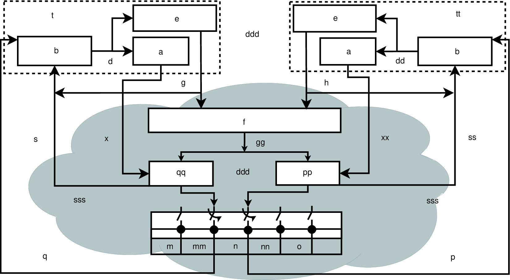
We consider an NCS consisting of $N$ synchronous stochastic linear time-invariant (LTI) controlled processes exchanging information over a common resource-limited communication network with resource management capabilities (see Fig. 1). Each process $i\!\in\mathrm{N}\!\triangleq\!\{1,\ldots,N\}$ comprises of a physical plant $\mathcal{P}_{i}$, a delay-sensitivity controller $\mathcal{S}_{i}$, and a feedback control unit consisting of a state feedback controller $\mathcal{C}_{i}$ and an estimator $\mathcal{E}_{i}$. The dynamics of the plant $\mathcal{P}_{i}$, $i\in\mathrm{N}$, is described by the following stochastic difference equation:

where $x^{i}_{k}\!\in\!\mathbb{R}^{n^{i}}$ represents sub-system $i$’s state vector at time-step $k\!\in\!\mathbb{N}\cup\{0\}$, $u^{i}_{k}\!\in\!\mathbb{R}^{m^{i}}\!$ denotes the corresponding control signal, $w^{i}_{k}\!\in\!\mathbb{R}^{n^{i}}$ the stochastic exogenous disturbance, and $A_{i}\!\in\!\mathbb{R}^{n^{i}\times n^{i}}$ and $B_{i}\!\in\!\mathbb{R}^{n^{i}\times m^{i}}$ describe the system and input matrices, respectively. To allow for heterogeneity, $A_{i}$ and $B_{i}$ matrices can be different across the NCS, i.e., $A_{i}\neq A_{j}$ and $B_{i}\!\neq\!B_{j}$, $i,j\!\in\!\mathrm{N}$. The disturbances are assumed to be random sequences with independent and identically distributed (i.i.d.) realizations $w^{i}_{k}\!\sim\!\mathcal{N}(0,\Sigma_{w}^{i})$, $\forall k$ and $i\!\in\!\mathrm{N}$, and $\Sigma_{w}^{i}\!\succ\!0$. The initial states $x^{i}_{0}$’s are also presumed to be randomly selected from any arbitrary finite-moment distributions with variance $\Sigma_{x_{0}}^{i}$. For simplicity, we assume that the sensor measurements are perfectly noiseless copies of the state values¹¹ 1 The results of this article extend, with lengthy but straightforward mathematical efforts, to noisy measurements if noise is an i.i.d. process..

In this section, we formulate a cross-layer joint optimization problem and discuss its structural characteristics w.r.t. to the policy makers. The three decision makers are 1) local plant controllers that computes the control input $u_{k}^{i},\;i\!\in\!\mathrm{N}$, at time-step $k$, 2) local delay controllers where the decision outcome $\theta_{k}^{i}$ determines the link $\ell_{d}\!\in\!\mathcal{L}$ through which $x_{k}^{i}$ will be transmitted, and 3) resource manager to compute $\vartheta_{k}^{i}$ that determines whether $\theta_{k}^{i}$ can be accordingly serviced.

We assume that individual control systems have no knowledge of each other’s parameters or decision variables. Let $\mathcal{I}_{k}^{i}$, $\mathcal{\bar{I}}_{k}^{i}$, and $\mathcal{\tilde{I}}_{k}$ denote the sets of accessible information for the plant controller, delay controller, and resource manager, respectively. (These sets are characterized in Section IV where the information structure at each policy maker is discussed.). Then, at every time $k$, the plant control, delay control, and resource allocation policies are measurable functions of the $\sigma$-algebras generated by their corresponding information sets, i.e., $u_{k}^{i}\!=\!\gamma_{k}^{i}(\mathcal{I}_{k}^{i})$, $\theta_{k}^{i}\!=\!\xi_{k}^{i}(\mathcal{\bar{I}}_{k}^{i})$, and $\vartheta_{k}\!=\!\pi_{k}(\mathcal{\tilde{I}}_{k})$. Note that, $\gamma^{i}$ and $\xi^{i}$ represent local policies corresponding to a specific sub-system $i$, while $\pi$ is computed centrally and includes the resource allocation profile for all $i\!\in\!\mathrm{N}$. The local objective function of each sub-system $i\!\in\!\mathrm{N}$, denoted by $J^{i}$, consists of its own LQG part plus the communication cost in average form over the finite horizon $[0,T]$, as follows:

where, $Q_{1}^{i}\!\succeq\!0$, $Q_{2}^{i}\!\succeq\!0$, and $R^{i}\!\succ\!0$ represent constant weight matrices for the state and control inputs, respectively.

The overall objective for the underlying NCS is to maximize the average performance of all sub-systems under the resource constraint (2). This cannot simply be obtained by taking the average of the sum of the local cost functions (7) because the local decision variable $\theta_{k}^{i}$ might not be realized due to the resource limitations. More precisely, the time that a state information is received at a controller might not always be the time decided by its delay controller. In fact, the cost function (7) is achievable for a certain sub-system $i$ only if $\vartheta_{k}^{i}=\theta_{k}^{i}$, $\forall k\!\in\![0,T]$. However, if the capacity of one or more transmission links are exceeded by the number of requests, the resource manager adjusts some of those requests, which eventually changes the realization of the control signal $u_{k}^{i}$ and consequently the value of the local cost $J^{i}(u^{i},\theta^{i})$.

We formulate the system (commonly called social) cost $J$ as the average difference between the sum of $J^{i}$’s from the resource manager (given $\vartheta_{k}^{i}$’s) and local sub-systems’ (given $\theta_{k}^{i}$’s) perspectives, i.e., knowing $\vartheta_{k}\!=\!\pi_{k}(\tilde{\mathcal{I}}_{k}\!)$, we have

and $J^{i}\!$ has been adjusted after resource allocation as

Note that, $J^{i}(u^{i},\theta^{i})$ is computed locally independent of the decisions for sub-systems $j\!\neq\!i$, while $J^{i}(u^{i},\vartheta^{i})$ is computed after central resource allocation is performed. The resources are allocated such that, w.r.t. the sub-systems preferences, the closest possible services are provided and $J$ is minimized.

In addition to the delay controllers that determine the per-time sensitivity of the control loops w.r.t. transmission latency, we introduce a constant latency-tolerance bound for each sub-system such that the resource manager allocates a transmission link only within that given bound. To diversify this static sensitivity for each sub-system, we define $\alpha_{i}$ and $\beta_{i}$ ($\in\!\mathcal{D}$) representing the maximum allowable delay tolerances. This specifies that a sub-system $i$ can tolerate imposed deviations by the network manager from the selected link $\ell_{d}$ only within the set $\{d-\alpha_{i},\ldots,d,\ldots,d+\beta_{i}\}$³³ 3 To avoid notational inconvenience, the network manager only takes into account the feasible tolerances of this set that also belong to $\mathcal{D}$. Moreover, for a nontrivial set, we assume at least one non-zero $\alpha_{i}$ and $\beta_{j}$, $i,j\in\mathrm{N}$.. The ultimate goal is then finding the optimal policies $\gamma_{k}^{i,\ast}(\mathcal{I}_{k}^{i})$, $\xi_{k}^{i,\ast}(\mathcal{\bar{I}}_{k}^{i})$ and $\pi_{k}^{\ast}(\mathcal{\tilde{I}}_{k})$ that jointly minimize the social cost $J$:

Constraint (10c) specifies that if at time $k$, $\theta_{k}^{i}(d)\!=\!1$, then the network manager allocates an available resource only from the set of links $\{\ell_{\max\{0,d-\alpha_{i}\}},\ldots,\ell_{\min\{d+\beta_{i},D\}}\}$ to sub-system $i$. The ultimate links from the allowable ones are selected by the resource manager such that the social cost $J$ is minimized. Note that problem (10) might not have a feasible solution for all $c_{d}$. We derive a sufficient feasibility condition in form of a lower bound for $c_{d}$ in the Section IV.

Solving problem (10) is challenging due to the couplings between the decision variables. In fact, $\theta_{k}^{i}$ is the best choice, from the perspective of sub-system $i$, to make the balance between its LQG cost and communication price. However, delay controller decisions may go through changes because of resource limitations. Note that, the control input $u_{k}^{i}$ is explicitly affected by $\theta_{k}^{i}$ in the absence of the resource limitations, but if $\vartheta_{k}^{i}\!\neq\!\theta_{k}^{i}$, then $u_{k}^{i}$ will have a different realization. This means the realization of $u_{k}^{i,\ast}$ computed from the problem (7) might be different from that being computed from the problem (9) even if both are computed from the same control law. Moreover, any decision of $\vartheta_{k}^{i}$ is clearly $\theta_{k}$-dependent. Further, as we discuss later, $\theta_{k+1}^{i}$ might also be a function of $\vartheta_{[0,k]}^{i}$. Altogether, problem (10) is nontrivial due to inter-dependencies and cross-layer constraints, hence we need to identify relevant conditions under which it can be decomposed.

Structural properties of the joint optimal policies are correlated with the cross-layer awareness model which characterizes the information sets $\mathcal{I}_{k}^{i},\bar{\mathcal{I}}_{k}^{i},\tilde{\mathcal{I}}_{k}$. We introduce different awareness models under which the couplings between $u_{k}^{i}$, $\theta_{k}^{i}$ and $\vartheta_{k}^{i}$ are examined. We discuss directed models of awareness for two different sets of information that can be exchanged between the decision makers of both layers: “constant model parameters” and “dynamic variables”. In the rest of the article, awareness of the constant model parameters for the network layer, if assumed, entails the knowledge of $\{A_{i},B_{i},Q_{1}^{i},Q_{2}^{i},R^{i},\Sigma_{w}^{i},\Sigma_{x_{0}}^{i}\},\forall i\!\in\!\mathrm{N}$. Note that, $\{\alpha_{i},\beta_{i}\}$’s are known to the network layer. The local delay and plant controllers are also assumed to have the knowledge of their own model parameters $\{A_{i},B_{i},Q_{1}^{i},Q_{2}^{i},R^{i},\Sigma_{w}^{i},\Sigma_{x_{0}}^{i},\alpha_{i},\beta_{i}\}$ as well as the constant network parameters $\{\Lambda,\mathcal{L}\}$.

To discuss awareness of dynamic variables, it is essential to have a clear picture of the order of generating variables in one sample cycle, e.g., $k\!\rightarrow\!k\!+\!1$. At the beginning of a sample time $k$, the system state $x_{k}^{i}$ is updated according to the dynamics (1), and then the delay controller generates $\theta_{k}^{i}$, based on the policy $\xi_{k}^{i}(\bar{\mathcal{I}}_{k}^{i})$ to determine the transmission link through which $x_{k}^{i}$ is to be communicated. System state $x_{k}^{i}$ together with the service request $\theta_{k}^{i}$ is then forwarded to the network to be serviced. The resource manager receives this information from all sub-systems and checks whether the number of requests for each link is exceeding its capacity. It then computes $\vartheta_{k}^{i}$, according to the policy $\pi_{k}(\tilde{\mathcal{I}}_{k})$, and $x_{k}^{i}$ is transmitted through the link determined by $\vartheta_{k}^{i}$. The control signal $u_{k}^{i}$ is computed from the control law $\gamma_{k}^{i}(\mathcal{I}_{k}^{i})$⁴⁴ 4 In case the information set $\mathcal{I}_{k}^{i}$ is not updated, i.e. if no new state information belonging to sub-system $i$ is scheduled to be delivered at time $k$, the control signal is updated based on a model-based estimation of $x_{k}^{i}$., $x_{k+1}^{i}$ is afterward updated and the pattern repeats over next samples.

At the controllers, the following awareness model of the dynamic variables is valid throughout the article. Knowledge of the model parameters of sub-system $i$ is assumed for $\mathcal{C}_{i}$. Reminding (6), the information set $\mathcal{I}_{k}^{i}$ at time $k$ is as

As in Fig. 2, the information set $\mathcal{I}_{k}^{i}$ in (11) specifies that the plant controllers are aware of the outcomes of the other two policies $\xi_{[0,k]}^{i}$ and $\pi_{[0,k]}^{i}$, from $t\!=\!0$ up to current time $t\!=\!k$. For that, we assume a dedicated low-bandwidth and error-free acknowledgement channel exists to inform the controllers at every time $k$ about $\theta_{k}^{i}$ and $\vartheta^{i}_{k}$ (see Fig. 1).

To determine the awareness structure for the resource manager, we consider the following assumption:

Assumption 1: The resource allocation law $\pi_{k}$ is rendered independent of the local plant control policies $\gamma_{[0,k-1]}^{i}$, $i\!\in\!\mathrm{N}$.

Assumption 1 declares a one-directional dependence between the plant control and resource allocation policies (see Fig. 2), i.e., $\gamma_{k}^{i}$’s are explicit functions of $\vartheta_{k}^{i}$, but $\pi_{k}$ does not incorporate $u_{[0,k-1]}^{i}$’s, $i\!\in\!\mathrm{N}$, in determining $\vartheta_{k}^{i}$. Although this results in the resource allocation being independent of local control laws, $\pi_{k}$ depends on $\theta_{[0,k]}^{i}$ which itself is effected by the control signals. In other words, the local delay controllers generate $\theta_{k}^{i}$’s such that an averaged equilibrium is achieved between maximizing the control performance and minimizing the communication cost. Since $\pi_{k}$ is an explicit function of $\theta_{[0,k]}^{i}$’s, the effect of optimizing control performance is indirectly considered in resource allocation. hence, the explicit dependence between the plant control and the resource manager policies that requires full knowledge of $u_{[0,k-1]}^{i}$’s, $i\!\in\!\mathrm{N}$ at the resource manager, is avoided. This assumption, nonetheless, leads to a considerable complexity reduction in computing the optimal policies $\pi_{k}^{\ast}$ and $\gamma_{k}^{i,\ast}$ (Section IV-A).

Having Assumption 1, we introduce the dynamic variables included in the resource manager’s information set $\tilde{\mathcal{I}}_{k}$, as

We also discuss the resource allocation with (Sec. IV-B) and without (Sec. IV-C) knowledge of the control systems model parameters. For the purpose of comparison, we discuss the scenario that the network manager does not take into account the local delay sensitivities in computing $\vartheta_{k}^{i}$’s, i.e., it allocates resources among sub-systems knowing neither the constant $\{\alpha_{i},\beta_{i}\}$’s nor $\theta^{i}_{[0,k]}$’s, $\forall i\in\mathrm{N}$ (see Sec. IV-D). This is an important observation which shows how the local and social cost functions change w.r.t. the individual delay sensitivities.

For delay controllers, we introduce two design approaches, so called impassive and reactive delay control policies, each representing a distinct model of awareness of the dynamic variables (Fig. 2). We derive the resulting joint optimal delay control and resource allocation policies in Sections IV-B and IV-C. Before that, to determine the structure of the optimal plant control policy $\gamma_{k}^{i,\ast}$, $i\!\in\!\mathrm{N}$, we need to introduce the maximum amount of information that can be available at the $i^{\textsf{th}}$ delay controller at a time $k$⁵⁵ 5 Later we discuss that (13) corresponds to the reactive delay control approach and introduce the information set for the impassive approach.. The set $\bar{\mathcal{I}}_{k}^{i}$ contains, at most, information about the following dynamic variables:

References

- [1] E. Molina and E. Jacob, “Software-defined networking in cyber-physical systems: A survey,” Computers and Electrical Engineering, vol. 66, pp. 407–419, 2018.
- [2] B. Bordel, R. Alcarria, T. Robles, and D. Martín, “Cyber-physical systems: Extending pervasive sensing from control theory to the internet of things,” Pervasive and Mobile Computing, vol. 40, pp. 156–184, 2017.
- [3] J. S. Baras, “A fresh look at network science: Interdependent multigraphs models inspired from statistical physics,” in 6th International Symposium on Communications, Control and Signal Processing, pp. 497–500, 2014.
- [4] D. Maity, M. H. Mamduhi, S. Hirche, K. H. Johansson, and J. S. Baras, “Optimal LQG control under delay-dependent costly information,” IEEE Control Systems Letters, vol. 3, pp. 102–107, Jan 2019.
- [5] J. Baillieul and P. J. Antsaklis, “Control and communication challenges in networked real-time systems,” Proceedings of the IEEE, vol. 95, no. 1, pp. 9–28, 2007.
- [6] S. Shakkottai, T. S. Rappaport, and P. C. Karlsson, “Cross-layer design for wireless networks,” IEEE Communications Magazine, vol. 41, no. 10, pp. 74–80, 2003.
- [7] J. Bai, E. P. Eyisi, F. Qiu, Y. Xue, and X. D. Koutsoukos, “Optimal cross-layer design of sampling rate adaptation and network scheduling for wireless networked control systems,” in Proceedings of 3rd International Conference on Cyber-Physical Systems, pp. 107–116, 2012.
- [8] F. Xia, “QoS challenges and opportunities in wireless sensor/actuator networks,” Sensors, vol. 8, no. 2, pp. 1099–1110, 2008.
- [9] M. A. Yigitel, O. D. Incel, and C. Ersoy, “QoS-aware MAC protocols for wireless sensor networks: A survey,” Computer Networks, vol. 55, no. 8, pp. 1982 – 2004, 2011.
- [10] A. Rajandekar and B. Sikdar, “A survey of MAC layer issues and protocols for machine-to-machine communications,” IEEE Internet of Things Journal, vol. 2, no. 2, pp. 175–186, 2015.
- [11] Y. Bi, L. X. Cai, X. S. Shen, and H. Zhao, “Medium access control for QoS provisioning in V2I communication networks,” Mobile Networks and Applications, vol. 18, no. 2, pp. 174–185, 2013.
- [12] K. B. Letaief and Ying Jun Zhang, “Dynamic multiuser resource allocation and adaptation for wireless systems,” IEEE Wireless Communications, vol. 13, no. 4, pp. 38–47, 2006.
- [13] Guocong Song and Ye Li, “Utility-based resource allocation and scheduling in OFDM-based wireless broadband networks,” IEEE Communications Magazine, vol. 43, no. 12, pp. 127–134, 2005.
- [14] Q. Zhang and Y. Zhang, “Cross-layer design for QoS support in multihop wireless networks,” IEEE Proceedings, vol. 96, no. 1, pp. 64–76, 2008.
- [15] B. Li, Y. Ma, T. Westenbroek, C. Wu, H. Gonzalez, and C. Lu, “Wireless routing and control: A cyber-physical case study,” in 7th International Conference on Cyber-Physical Systems, pp. 1–10, 2016.
- [16] H. Susanto and B. G. Kim, “Congestion control with QoS and delays utility function,” in 22nd International Conference on Computer Communication and Networks, pp. 1–5, 2013.
- [17] H. Wang, C. Liao, and Z. Tian, “Providing quality of service over time delay networks by efficient queue management,” in IEEE 36th Conference on Local Computer Networks, pp. 275–278, 2011.
- [18] F. Forni, S. Galeani, D. Nesić, and L. Zaccarian, “Event-triggered transmission for linear control over communication channels,” Automatica, vol. 50, no. 2, pp. 490 – 498, 2014.
- [19] X. Wang and M. D. Lemmon, “Event-triggering in distributed networked control systems,” IEEE Transactions on Automatic Control, vol. 56, no. 3, pp. 586–601, 2011.
- [20] G. S. Seyboth, D. V. Dimarogonas, K. H. Johansson, P. Frasca, and F. Allgöwer, “On robust synchronization of heterogeneous linear multi-agent systems with static couplings,” Automatica, vol. 53, pp. 392–399, 2015.
- [21] D. Maity and J. S. Baras, “Optimal event-triggered control of nondeterministic linear systems,” IEEE Transactions on Automatic Control, vol. 65, no. 2, pp. 604–619, 2020.
- [22] W. P. M. H. Heemels, K. H. Johansson, and P. Tabuada, “An introduction to event-triggered and self-triggered control,” in 51st IEEE Conference on Decision and Control, pp. 3270–3285, 2012.
- [23] Y. Tang, H. Gao, and J. Kurths, “Robust self-triggered control of networked systems under packet dropouts,” IEEE Transactions on Cybernetics, vol. 46, pp. 3294–3305, Dec 2016.
- [24] K. Hashimoto, S. Adachi, and D. V. Dimarogonas, “Self-triggered model predictive control for nonlinear input-affine dynamical systems via adaptive control samples selection,” IEEE Transactions on Automatic Control, vol. 62, no. 1, pp. 177–189, 2017.
- [25] S. Trimpe, “Predictive and self triggering for event-based state estimation,” in 55th IEEE Conference on Decision and Control, pp. 3098–3105, 2016.
- [26] A. Molin and S. Hirche, “Price-based adaptive scheduling in multi-loop control systems with resource constraints,” IEEE Transactions on Automatic Control, vol. 59, no. 12, pp. 3282–3295, 2014.
- [27] W. P. M. H. Heemels, A. R. Teel, N. van de Wouw, and D. Nesić, “Networked control systems with communication constraints: Tradeoffs between transmission intervals, delays and performance,” IEEE Transactions on Automatic Control, vol. 55, no. 8, pp. 1781–1796, 2010.
- [28] M. H. Mamduhi, D. Tolić, A. Molin, and S. Hirche, “Event-triggered scheduling for stochastic multi-loop networked control systems with packet dropouts,” in 53rd IEEE Conference on Decision and Control, pp. 2776–2782, 2014.
- [29] K. Okano, M. Wakaiki, G. Yang, and J. Hespanha, “Stabilization of networked control systems under clock offsets and quantization,” IEEE Transactions on Automatic Control, vol. 63, no. 6, pp. 1708–1723, 2018.
- [30] B. Demirel, V. Gupta, D. E. Quevedo, and M. Johansson, “Threshold optimization of event-triggered multi-loop control systems,” in 13th International Workshop on Discrete Event Systems, pp. 203–210, 2016.
- [31] D. Yue, E. Tian, and Q. Han, “A delay system method for designing event-triggered controllers of networked control systems,” IEEE Transactions on Automatic Control, vol. 58, no. 2, pp. 475–481, 2013.
- [32] A. Molin and S. Hirche, “A bi-level approach for the design of event-triggered control systems over a shared network,” Discrete Event Dynamic Systems, vol. 24, pp. 153–171, Jun 2014.
- [33] B. W. Carabelli, R. Blind, F. Dürr, and K. Rothermel, “State-dependent priority scheduling for networked control systems,” in American Control Conference, pp. 1003–1010, 2017.
- [34] M. H. Mamduhi, A. Molin, D. Tolić, and S. Hirche, “Error-dependent data scheduling in resource-aware multi-loop networked control systems,” Automatica, vol. 81, pp. 209 – 216, 2017.
Appendix
-A Proof of Theorem 1
Proof:
To compute , the resource manager has no knowledge of , but incorporates ’s, , via . The controller knows about , and via , while , and are known for the delay controller via . From (7)-(8), we re-state (10) as