Shunki Kyoya and Kenji Yamanishi
Mixture Complexity and Its Application to Gradual Clustering Change Detection
Abstract
In model-based clustering using finite mixture models, it is a significant challenge to determine the number of clusters (cluster size). It used to be equal to the number of mixture components (mixture size); however, this may not be valid in the presence of overlaps or weight biases. In this study, we propose to continuously measure the cluster size in a mixture model by a new concept called mixture complexity (MC). It is formally defined from the viewpoint of information theory and can be seen as a natural extension of the cluster size considering overlap and weight bias. Subsequently, we apply MC to the issue of gradual clustering change detection. Conventionally, clustering changes has been considered to be abrupt, induced by the changes in the mixture size or cluster size. Meanwhile, we consider the clustering changes to be gradual in terms of MC; it has the benefits of finding the changes earlier and discerning the significant and insignificant changes. We further demonstrate that the MC can be decomposed according to the hierarchical structures of the mixture models; it helps us to analyze the detail of substructures.
keywords
Finite mixture model, Clustering, Change detection, Gradual change, Information theory1 Introduction
As an introduction, we first state our interest and roughly introduce the concept of mixture complexity. Then, we discuss its related work and significance.
1.1 Motivation
Finite mixture models are widely used for model-based clustering (for overviews and references see McLachlan and Peel 2000; Fraley and Raftery 1998). In this field, it is a classical issue to determine the number of components. It has the following two meanings: the number of elements to represent the density distribution and the number of clusters to group the data (referred to as mixture size and cluster size, respectively). In this study, we consider the problem of estimating the cluster size when the mixture size is given. The cluster size used to be equal to the mixture size; however, it may not be valid when the components have overlaps or weight biases. Therefore, we need to reconsider the definitions and meanings of the cluster size.
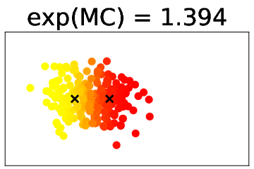
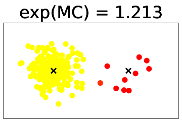
For instance, let us observe three cases of the Gaussian mixture model, as shown in Figure 1. Although the mixture size is two in any case, the situations are different. In case (a), the two components are distinct from each other and their weights are not biased; then, there seems to be no problem to believe that the cluster size is two as well. Meanwhile, in case (b), although their weights are not biased, the two components are very close to each other; then, as proposed in Hennig 2010, we may need to regard them as one cluster by merging them. In case (c), although the two components are distinct from each other, their weights are biased; then, as proposed in Jiang et al. 2001 and He et al. 2003, we may need to regard the small component as outliers rather than a cluster. Overall, in cases (b) and (c), it may be more difficult to say that the cluster size is exactly two than that in case (a). This observation gives rise to the problem of formally defining the complexity of clustering structures that reflects the overlaps and weight biases.
This paper introduces a novel concept of mixture complexity (MC) to resolve this problem. It is related to the logarithm of the cluster size. For example, the exponentials of the MC are 2.00, 1.39, 1.21 for cases (a), (b), and (c), respectively. In other words, given the mixture size, MC estimates the cluster size continuously rather than discretely.

There are two reasons for the need of MC. First, it theoretically evaluates the cluster size in the finite mixture model considering the overlap and imbalance between the components. Although their impacts on the cluster size have been discussed independently, we present a unified framework to interpret the cluster size by a continuous index. It presents a new perspective on model-based clustering and can be practically applied to cluster merging or clustering-based outlier detection. The second is the application of MC to the issue of gradual clustering change detection. Conventionally, clustering changes have been considered to be abrupt, induced by the changes in the mixture size or cluster size. In reality, however, there are cases where mechanisms for generating data change gradually (or incrementally in the context of concept drifts (Gama et al. 2014)). We thereby present a new methodology for tracking such changes by observing MC’s changes.
We further show that MC can be used to quantify the cluster size in hierarchical mixture models. We demonstrate that the MC of a hierarchical mixture model can be decomposed into the sum of MCs for local mixture models. It enables us to evaluate the complexity of the substructures as well as the entire structure.
1.2 Related Work
The issue of determining the best mixture size or cluster size (often referred to as model selection) has extensively been studied. For example, AIC (Akaike 1974), BIC (Schwarz 1978), and MDL (Rissanen 1978) have been used to select the mixture size; ICL (Biernacki et al. 2000) and MDL-based clustering criterion (Kontkanen et al. 2005; Hirai and Yamanishi 2013; Hirai and Yamanishi 2019) have been invented to select the cluster size. See also a recent review by McLachlan and Rathnayake 2014 focusing on the number of components in a Gaussian mixture model.
Differences between the mixture size and cluster size have also been widely discussed. For example, McLachlan and Peel 2000 pointed out that there were cases that Gaussian mixture models with more than one mixture sizes were needed to describe one skewed cluster; Biernacki et al. 2000 argued that in many situations, the mixture size estimated by BIC was too large to regard it as the cluster size. The problem of estimating the cluster size under a given mixture size has also been investigated by Hennig 2010; he proposed methods to identify the cluster structure by merging heavily overlapped mixture components. MC differs from his approach in that it interprets the clustering structure by only measuring the overlap rate rather than deciding whether to merge based on a certain threshold.
The degree of overlap or closeness between components has been evaluated using various measures, such as the classification error rate or the Bhattacharyya distance (Fukunaga 1990). Wang and Sun 2004 and Sun and Wang 2011 formulated the overlap rate of Gaussian distributions from the geometric nature of them. All of the works above have been limited to the case of two components. On the other hand, MC considers the overlap between any number of components.
Deciding whether a small component is a cluster or a set of outliers is also a significant matter. For example, clustering algorithms such as DBSCAN (Ester et al. 1996) and constrained -means (Bradley et al. 2000) avoided generating small components to obtain a better clustering structure. Jiang et al. 2001 and He et al. 2003 associated the small components with outlier detection problems. MC evaluates the small components by continuously measuring the impacts on the cluster size.
Some other notions have been proposed to quantify the clustering structure. Rusch et al. 2018 evaluated the crowdedness of the data under the concept of “clusteredness.” However, its relations to the cluster size are indirect. Recently, descriptive dimensionality (Ddim) (Yamanishi 2019) was proposed to define the model dimensionality continuously. It can be implemented to estimate the clustering structure under the assumption of model fusion, that is, models with different number of components are probabilistically mixed. MC differs from Ddim because it evaluates the overlap and weight bias in the single model without the model fusion.
Clustering under the data stream has been discussed with various objectives (Guha et al. 2000; Song and Wang 2005; Chakrabarti et al. 2006). We consider the problem of detecting changes in the cluster structure; Dynamic model selection (DMS) (Yamanishi and Maruyama 2005; Yamanishi and Maruyama 2007; Hirai and Yamanishi 2012) addressed this problem by observing the changes in the models (corresponding to mixture size or cluster size in this paper). Because the models are valued discretely, the detected changes have been considered to be abrupt. Refer also to the notions of tracking best experts (Herbster and Warmuth 1998), evolution graph (Ntoutsi et al. 2012), and switching distributions (van Erven et al. 2012), which are similar to DMS.
Furthermore, the issues of gradual changes have been discussed to investigate the transition periods for absolute changes. The MDL change statistics (Yamanishi and Miyaguchi 2016) was proposed to measure the degree of gradual changes. The notions of structural entropy (Hirai and Yamanishi 2018) and graph entropy (Ohsawa 2018) were proposed to measure the degree of model uncertainty in the changes. This study quantifies the degree of gradual changes by the fluctuations in MC and presents a new methodology to detect them.
1.3 Significance and novelty
The significance and novelty of this paper are summarized below.
Mixture complexity for finite mixture models.
We introduce a novel concept of MC to continuously measure the cluster size in a mixture model. It is formally defined from the viewpoint of information theory and can be interpreted as a natural extension of the cluster size considering the overlaps and weight biases among the components. We further demonstrate that MC can be decomposed into a sum of MCs according to the mixture hierarchies; it helps us in analyzing MC in a decomposed manner.
Applications of MC to gradual clustering change detection.
We apply MC to the issue of monitoring gradual changes in clustering structures. We propose methods to monitor changes in MC instead of the mixture size or cluster size. Because MC takes a real value, it is more suitable for observing gradual changes. We empirically demonstrate that MC elucidates the clustering structures and their changes more effectively than the mixture size or cluster size.
The remainder of this paper is organized as follows. In Section 2, we introduce the concept of MC. We also present some examples and theoretical properties. In Section 3, we show the decomposition properties of MC. Section 4 discusses an application of MC to clustering change detection problems and Section 5 describes the experimental results. Finally, Section 6 concludes this paper. Proofs of the propositions and theorems are described in Appendix A. Programs for the experiments are available at https://github.com/ShunkiKyoya/MixtureComplexity.
2 Mixture Complexity
In this section, we formally introduce the mixture complexity and describe its properties by some examples and theories.
2.1 Definitions
Given the data and the finite mixture model that have generated them, we consider estimating the cluster size of . The distribution is written as
where denotes the mixture size, denote the proportions of each component summing up to one, and denote the probability distributions. The random variable following the distribution is called an observed variable because it can be observed as a datum. We also define the latent variable as the index of the component from which the observed variable originated. The pair is called a complete variable. The distribution of the latent variable and the conditional distribution of the observed variable can be given by
To investigate the clustering structures in , we consider the following quantity:
where and denote the entropy and conditional entropy, respectively, of the latent variable defined as
The quantity is well-known as the mutual information between the observed and latent variables; it is also known as the (generalized) Jensen-Shannon Divergence (Lin 1991). We can interpret as the volume of cluster structures as follows. Because is a subtraction of the latent variable’s entropy with and without the knowledge of the observed variable, it represents the amount of information about the latent variable possessed by the observed data. Thus, its exponent denotes the “number” of clusters distinguished by the observed variable; it can be interpreted as a continuous extension of the cluster size. For more information about entropy and mutual information, see Cover and Thomas 2006, for example.
However, cannot be calculated analytically. Thus, we approximate using the data as follows:
where we assume that holds for all . We call this the MC of the mixture model .
Definition 1.
We define the MC of the mixture model and that with data weights as the quantities calculated as
| (1) |
and
respectively.
The weighted version of MC is used in Section 3.
Note that there are other ways to approximate ; we adopt the form of Equation (1) because it has the decomposition property shown in Section 3. See also methods to approximate the entropy of the mixture model (Huber et al. 2008; Kolchinsky and Tracey 2017) that can also be applied to approximate .
In practice, only the data can be obtained without the underlying distribution . Then, we estimate and from the data and further approximate the MC as
2.2 Examples
In this subsection, we discuss some examples of MC to understand its notions.
2.2.1 MC with different overlaps
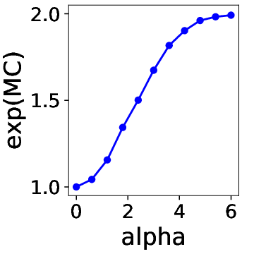
First, we set and generated the data as follows.
where denotes a multivariate normal distribution with mean and covariance , denotes a -dimensional identity matrix, and is the parameter that determines the degree of overlap between two components.
By varying the value of among 0, 0.6, …, 6.0, we generated the data and measured the MC by setting and as the actual distributions. The exponential of the MC for each is plotted in Figure 2(a). It is evident from the figure that the MC smoothly increases from 1.0 to 2.0 as the two components become isolated.
2.2.2 MC with different mixture biases
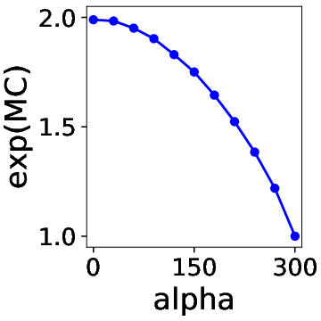
Next, we set and generated the data as follows:
where is the parameter that determines the degree of bias between the proportion of two components.
By varying among 0, 30, …, 300, we generated the data and measured the MC by setting and as the actual distributions. The exponential of the MC for each is plotted in Figure 2(b). It is evident from the figure that the MC smoothly decreases from 2.0 to 1.0 as the balance becomes biased.
2.3 Theoretical properties
In this subsection, we discuss the theoretical properties of MC. For simplicity, we does not consider the data weights here. Their proofs are described in Appendix A.
First, we show that if the components entirely overlap, MC becomes 0.
Proposition 2.
If , then
Next, we show the relation between MC and mixture size . If the components are entirely separated and balanced, MC becomes .
Proposition 3.
If there is only one index that satisfies for all and for all , then
In particular, if , then
We also show that if the proportions are estimated by maximizing the logarithm of the likelihood, 0 and are the lower and upper bounds of MC, respectively.
Proposition 4.
If are an optimal solution of the following problem:
then MC satisfies
Finally, we show that the value of MC is invariant with the representation of the mixture distribution. For example, consider the following three mixture distributions:
In and , we need to manually remove the redundant components and regard the mixture size as two (McLachlan and Peel 2000). On the other hand, the following property indicates that the MCs for , and are the same; thus, we need not to care about their differences in evaluating MC.
Proposition 5.
If two mixture distributions and are equivalent in the sense that
where is the Kronecker’s delta function on a function space containing and , then
3 Decomposition of MC
In this section, we discuss a method to decompose MC along the hierarchies in mixture models; this can help us in analyzing the structures in more detail.
Consider that the mixture distribution has a two-stage hierarchy, as shown in Figure 3. It has components on the lower side and components on the upper side, where denote the probability distributions and denote their mixture distributions, respectively. We construct the hierarchy as follows. First, we estimate the distribution . Then, we obtain by partitioning (or clustering) the lower components into groups. Formally, we denote as the proportion of the lower component that belongs to the upper component , which satisfies for all . Then, we derive by rewriting as
where

According to the hierarchy, we can decompose the MC.
Theorem 6.
We can decompose the MC as follows:
where
The proof is described in Appendix A.
For notational simplicity, we will use the following terms:
- •
: MC(total),
- •
: MC(interaction),
- •
: Contribution(component ),
- •
: W(component ),
- •
: MC(component ).
Then, we can rewrite Theorem 6 as
In Theorem 6, the MC of the entire structure (MC(total)) is decomposed into a sum of the MC among the upper components (MC(interaction)) and their respective contributions (Contribution(component )). Contribution(component ) is further decomposed into a product of the weight (W(component )) and complexity (MC(component )) of the component. Because denotes the weight of that belongs to component , its sum W(component ) represents the total weights of the data contained in it. Also, MC(component ) denotes the clustering structures in component considering the data weights.
An example of the decomposition is illustrated in Figure 4 and Table 1. In this example, there are lower components generated from a Gaussian mixture model; additionally, there are upper components on the left and right sides. By decomposing MC(total), we can evaluate the complexities in the local structures as well as those in the entire structure.


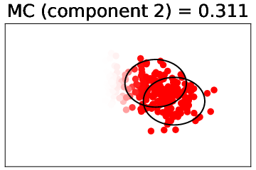
| component 1 | component 2 | |
| MC(total) | 1.076 | |
| MC(interaction) | 0.643 | |
| Contribution(component ) | 0.277 | 0.157 |
| W(component ) | 0.496 | 0.504 |
| MC(component ) | 0.558 | 0.311 |
4 Application to clustering change detection
In this section, we propose methods to apply the MC to clustering change detection problems. Formally speaking, given the dataset , where denotes the time and denote the data generated at each , we consider the problem of monitoring the changes in the clustering structures over .
First, we briefly summarize the method named sequential dynamic model selection (SDMS) (Hirai and Yamanishi 2012) that has addressed this problem. Then, we introduce our ideas and discuss the differences between SDMS.
Hereafter, we assume that the data points are -dimensional vectors and consider a Gaussian mixture model
for each .
4.1 Sequential dynamic model selection
SDMS is an algorithm that is used to sequentially estimate models and find changes. In clustering change detection problems, it sequentially estimates the mixture sizes and parameters and finds model changes as changes in .
The estimation procedures are explained below. First, depending on the estimated mixture size at the last time point , we set the candidate for . Then, for each in the candidate, we estimate the parameters from the data and calculate a cost function . Finally, we select as the mixture size that minimizes the costs. The candidate of are set as
at , and
at , where is a pre-defined parameter. The cost function denotes the sum of the code length functions of the model and model changes given by
Code length of the model
The score denotes a sum of the logarithm of the likelihood functions and penalty terms corresponding to the complexity of the model. In this study, we consider two likelihood functions and four penalty terms. For the (logarithm of) likelihood functions, we consider the observed likelihood and complete likelihood , given by
where are the latent variables for the data estimated by
They correspond to the likelihood of the observed data and complete data, respectively; the former is used to determine the mixture size, and the latter is used to determine the cluster size under the assumption that it is equal to the mixture size. For the penalty terms, we consider AIC (Akaike 1974), BIC (Schwarz 1978), NML (Hirai and Yamanishi 2013; Hirai and Yamanishi 2019), and DNML (Wu et al. 2017; Yamanishi et al. 2019). By combining the log-likelihood and the penalty terms, we consider the following six scores:
- •
AIC with observed likelihood (AIC): ,
- •
AIC with complete likelihood (AIC+comp): ,
- •
BIC with observed likelihood (BIC): ,
- •
BIC with complete likelihood (BIC+comp): ,
- •
NML: ,
- •
DNML: ,
where denotes the number of the free parameters required to represent a Gaussian mixture model; and denote the parametric complexities. In our experiments, we estimated the parameter by conducting the EM algorithm (Dempster et al. 1977) implemented in the Scikit-learn package (Pedregosa et al. 2011) ten times and choose the best parameter that minimized each score. Note that in NML and DNML, we only considered the complete likelihood functions because only the methods to calculate their parametric complexities are known.
Code length for model change
The code length for the model change can be written as
where denotes the probability of the model change, defined as
for all at and
at ; additionally, is a predefined parameter. In our experiments, we fixed .
4.2 Tracking MC
In SDMS, clustering changes are detected as the changes of the mixture size or cluster size ; because it is discrete, the changes have been considered to be abrupt. Then, we propose to track MC instead of while estimating the parameters by SDMS. Because MC takes a real value, monitoring it is more suitable for observing gradual changes than monitoring . The algorithm for tracking MC is explained in Algorithm 1.
4.3 Tracking MC with its decomposition
In addition to monitoring the MC of the entire structure, we also propose an algorithm to track its decomposition. To accomplish this, we must estimate the upper components and their corresponding partitions for each .
Here, we assume that the upper components are common at every and estimate the partition after estimating the lower components at each time. Specifically, we consider as a point with weights for each and and cluster them. As the clustering algorithm, we modified the fuzzy c-means (Bezdec et al. 1984) to handle the weighted points. Formally, we estimated the centers of the upper components and their corresponding partitions by minimizing the loss function
where is parameter that determines the fuzziness of the partition.
We estimated and by minimizing one iteratively while fixing another. We can formulate the iteration as follows:
Finally, we present an algorithm to track the MC and its decomposition in Algorithm 2. We can analyze the structural changes in more detail by evaluating the decomposed values.
5 Experimental results
In this section, we present the experimental results that demonstrate the MC’s abilities to monitor the clustering changes. We compare our methods to the monitoring of .
5.1 Analysis of artificial data
To reveal the behaviors of MC, we conducted experiments with two artificial datasets called move Gaussian dataset and imbalance Gaussian dataset. Their experimental designs are discussed below. First, we generated artificial datasets by setting and . The datasets have one transaction period in which the data change their clustering structures gradually. Then, we estimated the MC and using the methods in Subsections 4.2 and 4.1 by setting . To compare them, we first created a simple algorithm to detect the changes from the sequence of MC or . Then, we compared the abilities of this algorithm in terms of the speed and accuracy of detecting the change points. Moreover, to evaluate the abilities to find the changes in the opposite direction, we performed experiments with the same datasets in the reverse order.
Given a sequence of the MC or written as , we constructed an algorithm to detect the change points as follows. For , we raised a change alert if
in the case of MC, and
in the case of . We calculated the medians instead of the means of the subsequences for robustness. However, to avoid redundant alerts, we neglected them when the difference between and the latest alert was less than 5 even if the conditions were satisfied.
To evaluate the quality of the algorithm, we calculated Delay and False alarm rate (FAR), defined as
where denotes the first time point in the transaction period when the algorithm generated an alert, ACCEPT denotes the set of time points when alerts are allowed defined as , and ALERT denotes the set of time points when the algorithm generated alerts.
5.1.1 Move Gaussian dataset
The move Gaussian dataset is a set of three-dimensional Gaussian distributions, whose means move gradually in the transaction period. Formally, for each , we generated the data as follows:
where
The first and second dimensions of some data are visualized in Figure 5. In the direction , the number of clusters increases from two to three as the two clusters leave; in the direction , it decreases from three to two as the two clusters merge.


The experiments were performed ten times by randomly generating the datasets; accordingly, the average performance scores were calculated. The differences in the scores between the MC and for each criterion are presented in Table 2; the estimated MC and in one trial are proposed in Figure 6. This figure illustrates the result of BIC as an example.
With respect to the speed to find changes, in every criterion, MC performed as well as in the direction ; however, it performed significantly better than in the direction . The reason for the differing performances is discussed below. In the direction , the model selection algorithms underestimated the number of components at the beginning of the transaction period. In such time points, they ignored the overlapping of the two components and considered them as one cluster. Thus, MC, based on such model selection methods, was unable to find the changes earlier than . However, in the direction , the overlap between the components was correctly estimated at some time points before changed. In this case, MC changed smoothly according to the overlap and found changes earlier than .
With respect to the accuracy of finding changes, MC performed as well as in terms of FAR. Additionally, it is evident from Figure 6 that MC stably estimated the clustering structures.


| (score of MC) - (score of ) | ||||
| criterion | Delay | FAR | Delay | Far |
| AIC | 0.0 | 0.000 | -20.6 | 0.000 |
| AIC+comp | 0.0 | 0.000 | -10.9 | 0.000 |
| BIC | 0.0 | 0.000 | -17.5 | 0.000 |
| BIC+comp | 0.0 | 0.000 | -8.9 | 0.000 |
| NML | 0.0 | 0.000 | -7.9 | 0.000 |
| DNML | 0.0 | 0.000 | -7.7 | 0.000 |
5.1.2 Imbalance Gaussian dataset
The imbalance Gaussian dataset is a set of three-dimensional Gaussian mixture distributions whose balances change gradually in the transaction period. Formally, for each , we generated the data as follows:
where
The first and second dimensions of some data are visualized in Figure 7. In the direction , the number of clusters decreases from four to three as the edge cluster disappears. In the direction , it increases from three to four as the edge cluster emerges.


The experiments were performed ten times by randomly generating datasets; accordingly, the average performance scores were calculated. The difference in the scores between the MC and for each criterion are listed in Table 3. The estimated MC and in one trial are plotted in Figure 8. This figure illustrates the result of BIC as an example.
In terms of the speed to find changes, in every model selection method, MC performed significantly better than in the direction ; however, MC performed as well as in the direction . The reason for the differing performances is discussed below. In the transaction period, all model selection methods counted the minor components as independent clusters. Then, in the direction , MC changed smoothly according to the imbalance and determined the changes earlier than . In the direction , increased significantly early in the transaction period. Then, MC increased along with and determined the changes simultaneously.
In terms of the accuracy of finding changes, MC performed as well as in terms of FAR. Additionally, it is evident from Figure 8 that MC stably estimated the clustering structures.


| (score of MC) - (score of ) | ||||
| criterion | Delay | FAR | Delay | Far |
| AIC | -30.2 | 0.010 | -4.6 | 0.000 |
| AIC+comp | -34.0 | 0.000 | 0.0 | 0.000 |
| BIC | -34.0 | 0.000 | 0.0 | 0.000 |
| BIC+comp | -34.0 | 0.000 | 0.0 | 0.000 |
| NML | -34.0 | 0.000 | 0.0 | 0.000 |
| DNML | -34.0 | 0.000 | 0.0 | 0.000 |
5.2 Analysis of real data
We analyzed two types of real data named the beer dataset and house dataset, which are summarized in Table 4. In the following subsections, we discuss the detail of the datasets and results of the experiments.
| dataset | description | |||
|---|---|---|---|---|
| beer | 92 | 3185 | 16 | purchase data of beer. |
| house | 96 | 4326 | 3 | electricity consumption data in a house. |
5.2.1 Beer dataset
We discuss the results of the beer dataset, obtained from Hakuhodo, Inc. and M-CUBE, Inc. The dataset comprises the records of customer’s beer purchases from November 1st, 2010 to January 31th, 2011. The dataset is constructed as follows. The time unit is a day. For each day , denotes the -th customer’s consumption of the beer from time to , where we set . The dimension of the vector is 16, which correspond to the consumptions of the following drink:
- •
beer(A), …, beer(F): beer with brand name A, …, F.
- •
beer(other): beer with other brands.
- •
beerlike(A), …, beerlike(H): beer-like drink with brand name A, …, H.
- •
beerlike(other): beer-like drink with other brands.
First, we compare the plots of the estimated MC and in Figure 9. The results of BIC and NML are illustrated as an example. In any method, the score was high at the end and beginning of the year, reflecting the increased activities in transactions. However, because the critical changes in the clustering structure and changes due to ineffective components were mixed, the sequence of had a lot of change points and was difficult to interpret their meanings. On the other hand, MC identified the clustering structure by discounting the effects of the ineffective components. As a result, the sequence of MC highlighted the significant changes at the end and beginning of the year. It is also worthwhile noting that the differences of the scores between the model selection methods were much smaller in MC than those in ; it indicates that both BIC and NML estimates the similar clustering structure under the concept of MC even though the number of components differs significantly.

Next, we discuss the results of the decomposition of MC. We present the results of BIC and NML with and . The centers of the upper components are listed in Table 5 and Table 6, respectively, and the plots of each decomposed value are illustrated in Figure 10 and Figure 11, respectively. The indices of the upper components are manually rearranged so that they correspond with each other; then, it can be observed that the results were also similar to each other. The structures can be extensively evaluated by analyzing the decomposed values. For instance, let us analyze the decomposed values at the end and beginning of the year. As evident from the tables, they had different characteristics. It can be observed from the figures that the contributions increased in all components, indicating that they were related to the increase in MC(total). The weight of the component decreased in cluster 1 and increased in component 2 and 3, indicating that the customers moved from component 1 to component 2 and 3. Also, MC(component ) increased in all components, indicating that the complexity or diversity increased within them.
| component 1 | component 2 | component 3 | component 4 | |
|---|---|---|---|---|
| beer(A) | 0.09 | 0.44 | 1.93 | 0.16 |
| beer(B) | 0.07 | 0.23 | 0.96 | 0.06 |
| beer(C) | 0.07 | 0.20 | 0.83 | 0.07 |
| beer(D) | 0.05 | 0.20 | 0.58 | 0.05 |
| beer(E) | 0.03 | 0.06 | 0.35 | 0.03 |
| beer(F) | 0.03 | 0.06 | 0.35 | 0.02 |
| beer(other) | 0.04 | 0.12 | 0.69 | 0.10 |
| beerlike(A) | 0.02 | 5.85 | 0.23 | 0.07 |
| beerlike(B) | 0.09 | 0.57 | 0.80 | 0.21 |
| beerlike(C) | 0.10 | 0.63 | 0.83 | 0.22 |
| beerlike(D) | 0.07 | 0.40 | 0.57 | 0.18 |
| beerlike(E) | 0.04 | 0.12 | 0.51 | 0.06 |
| beerlike(F) | 0.04 | 0.20 | 0.34 | 0.13 |
| beerlike(G) | 0.05 | 0.10 | 0.40 | 0.06 |
| beerlike(H) | 0.03 | 0.09 | 0.26 | 0.04 |
| beerlike(other) | 0.09 | 1.27 | 1.11 | 6.78 |
| component 1 | component 2 | component 3 | component 4 | |
|---|---|---|---|---|
| beer(A) | 0.08 | 0.48 | 1.90 | 0.12 |
| beer(B) | 0.04 | 0.30 | 1.04 | 0.07 |
| beer(C) | 0.05 | 0.20 | 0.95 | 0.04 |
| beer(D) | 0.04 | 0.19 | 0.64 | 0.09 |
| beer(E) | 0.02 | 0.06 | 0.38 | 0.02 |
| beer(F) | 0.02 | 0.07 | 0.40 | 0.01 |
| beer(other) | 0.03 | 0.11 | 0.68 | 0.19 |
| beerlike(A) | 0.02 | 5.79 | 0.21 | 0.07 |
| beerlike(B) | 0.10 | 0.52 | 0.73 | 0.18 |
| beerlike(C) | 0.11 | 0.61 | 0.70 | 0.21 |
| beerlike(D) | 0.06 | 0.49 | 0.52 | 0.24 |
| beerlike(E) | 0.04 | 0.12 | 0.47 | 0.07 |
| beerlike(F) | 0.04 | 0.18 | 0.30 | 0.24 |
| beerlike(G) | 0.04 | 0.11 | 0.44 | 0.07 |
| beerlike(H) | 0.02 | 0.10 | 0.23 | 0.09 |
| beerlike(other) | 0.08 | 1.42 | 1.08 | 6.54 |


5.2.2 House dataset
We discuss the results of the house dataset, obtained from the UCI Machine Learning Repository (Dheeru and Casey 2017). The dataset comprises the records of electricity consumption in a house every five minutes from December 16th, 2006 to November 26th, 2010. The dataset is constructed as follows. The time unit is 15 minutes from 00:00-00:15 to 23:45-24:00. For each , the data denotes the set of the records on the various days included in the -th time unit. The dimension of the vector is 3, which corresponds to the metering of the following three points:
- •
metering(A): a kitchen.
- •
metering(B): a laundry room.
- •
metering(C): a water-heater and an air-conditioner.
First, we compare the plots of the estimated and the corresponding MC in Figure 12. The results of BIC and NML are illustrated as an example. It can be observed from the figure that the MC smoothly connected the discrete changes in ; therefore, MC expressed gradual changes in the dataset more effectively than . Also, the MCs in BIC and NML were more similar each other than as well as in the beer dataset. The values of MC started increasing from around 7:00 a.m.; after slight fluctuations, the value reached its peak around 21:00. Therefore, MC seemed to represent the amount of activities in this house.

Next, we discuss the results of the decomposition of MC. We present the results of BIC and NML with and . The centers of the upper components are listed in Table 7 and Table 8, respectively, and the plots of each decomposed value are illustrated in Figure 13 and Figure 14, respectively. The indices of the upper components are manually rearranged so that they correspond with each other; then, it can be observed that the results were also similar to each other. The structures can be extensively evaluated by analyzing the decomposed values. For instance, let us analyze the decomposed values in component 3. It can be observed from the tables that the value in metering(C) was specifically high in this component. Looking at contribution(component 3), there were two peaks around 9:00 and 21:00; it represented the increased activities in this component. However, the proportions of the weight and MC were different. W(component 3) was specifically high at 9:00, indicating that the first half of the peaks was due to the increase in the weight of the component; whereas, MC(component 3) was specifically high at 21:00, indicating that the second half of the peaks was due to the increase in the complexity within the component.
| component 1 | component 2 | component 3 | component 4 | |
|---|---|---|---|---|
| metering(A) | 0.04 | 4.47 | 0.13 | 0.41 |
| metering(B) | 0.53 | 0.89 | 0.56 | 4.40 |
| metering(C) | 0.75 | 3.34 | 4.37 | 2.96 |
| component 1 | component 2 | component 3 | component 4 | |
|---|---|---|---|---|
| metering(A) | 0.04 | 4.24 | 0.11 | 0.35 |
| metering(B) | 0.53 | 1.00 | 0.57 | 4.48 |
| metering(C) | 0.76 | 3.37 | 4.38 | 2.93 |


6 Conclusion
We proposed the concept of MC to measure the cluster size continuously in the mixture model. We first pointed out that the cluster size might not be equal to the mixture size when the mixture model had overlap or weight bias; then, we introduced MC as an extended concept of the cluster size considering the effects of them. We also presented methods to decompose the MC according to the mixture hierarchies, which helped us in extensively analyzing the substructures. Subsequently, we implemented the MC and its decomposition to the gradual clustering change detection problems. We conducted experiments to verify that the MC effectively elucidate the clustering changes. In the artificial data experiments, MC found the clustering changes significantly earlier in the case where the overlap or weight bias was correctly estimated. In the real data experiments, MC expressed the gradual changes better than because it discerned the significant and insignificant changes and smoothly connected the discrete changes in . We also found that the MC took similar values for each model selection method; it indicates that the estimated clustering structures are alike under the concept of MC. Moreover, its decomposition enabled us to evaluate the contents of changes.
Issues of the MC will be tackled in future study. For example, it does not capture the clustering structure well when the number of the components is underestimated; thus, we need to explore the model selection methods that are more compatible with MC. Also, we further need to study its theoretical aspects, such as convergence and methods for approximating the mutual information.
Acknowledgement
The marketing dataset was provided by Hakuhodo, Inc. and M-CUBE, inc. This work was partially supported by JST KAKENHI 191400000190 and JST-AIP JPMJCR19U4.
Appendix A Proofs
In this section, we describe the proofs of the propositions and theorem stated in the text.
A.1 Proof of Proposition 2
Proof.
If , then
∎
A.2 Proof of Proposition 3
Proof.
We see from the assumption that
where . Note that there are no problems even when because in this case. Then, we can calculate the MC as
∎
A.3 Proof of Proposition 4
Proof.
For all , we derive as
Moreover, we see from the Karush-Kuhn-Tucker condition that
From this, we derive as
∎
A.4 Proof of Proposition 5
Proof.
It follows from the fact that
∎
A.5 Proof of Theorem 6
Proof.
We can directly calculate as
∎
References
- Akaike (1974) Hirotugu Akaike. A new look at the statistical model identification. IEEE Transactions on Automatic Control, 19(6):716–723, 1974.
- Bezdec et al. (1984) James C. Bezdec, Robert Ehrlich, and Willian Full. FCM: The fuzzy c-means clustering algorithm. Computers and Geosciences, 10(2–3):191–203, 1984.
- Biernacki et al. (2000) Christophe Biernacki, Gilles Celeux, and Gérard Govaert. Assessing a mixture model for clustering with the integrated completed likelihood. IEEE Transactions on Pattern Analysis and Machine Intelligence, 22(7):719–725, 2000.
- Bradley et al. (2000) Paul S. Bradley, Kristin P. Bennett, and Ayhan Demiriz. Constrained k-means clustering. Technical Report MSR-TR-2000-65, Microsoft Research, Redmond, Washington, 2000.
- Chakrabarti et al. (2006) Deepayan Chakrabarti, Ravi Kumar, and Andrew Tomins. Evorutionary clustering. In Proceedings of the 12th ACM SIGKDD International Conference on Knowledge Discovery and Data Mining, pages 554–560, Philadelphia, Pennsylvania, 2006.
- Cover and Thomas (2006) Thomas M. Cover and Joy A. Thomas. Elements of Information Theory (Wiley Series in Telecommunications and Signal Processing). Wiley-Interscience, New York, 2006.
- Dempster et al. (1977) Arthur P. Dempster, Nan M. Laird, and Donald B. Rubin. Maximum likelihood from incomplete data via the EM algorithm. Journal of the Royal Statistical Society. Series B (Methodological), 39(1):1–38, 1977.
- Dheeru and Casey (2017) Dua Dheeru and Graff Casey. UCI machine learning repository, 2017. URL http://archive.ics.uci.edu/ml.
- Ester et al. (1996) Martin Ester, Hans-Peter Krigel, Jorg Sander, and Xiaowei Xu. A density-based algorithm for discovering clusters in large spatial databases with noise. In Proceedings of the Second International Conference on Knowledge Discovery and Data Mining, pages 226–231, Portland, Oregon, 1996.
- Fraley and Raftery (1998) Chris Fraley and Ardian E. Raftery. How many clusters? which clustering method? answers via model-based cluster analysis. The Computer Journal, 41(8):578–588, 1998.
- Fukunaga (1990) Keinosuke Fukunaga. Introduction to Statistical Pattern Recognition (2nd Edition). Academic Press Professional, San diego, California, 1990.
- Gama et al. (2014) João Gama, Indrė Žliobaitė, Albert Bifet, Mykola Pechenizkiy, and Abdelhamid Bouchachia. A survey on concept drift adaptation. ACM Computing Surveys, 46(4):1–37, 2014.
- Guha et al. (2000) Sudipto Guha, Nina Mishra, Rajeev Motwani, and Liadan O’Callaghan. Clustering data streams. In Proceedings 41st Annual Symposium on Foundations of Computer, pages 359–366, Redondo Beach, California, 2000.
- He et al. (2003) Zengyou He, Xiaofei Xu, and Shengchun Deng. Discovering cluster-based local outliers. Pattern Recognition Letters, 24(9–10):1641–1650, 2003.
- Hennig (2010) Christian Hennig. Methods for merging Gaussian mixture components. Advances in Data Analysis and Classification, 4:3–34, 2010.
- Herbster and Warmuth (1998) Mark Herbster and Manfred K. Warmuth. Tracking the best expert. Machine Learning, 1998(32):151–178, 1998.
- Hirai and Yamanishi (2012) So Hirai and Kenji Yamanishi. Detecting changes of clustering structures using normalized maximum likelihood coding. In Proceedings of the 18th ACM SIGKDD International Conference on Knowledge Discovery and Data Mining, pages 343–351, Beijing, China, 2012.
- Hirai and Yamanishi (2013) So Hirai and Kenji Yamanishi. Efficient computation of normalized maximum likelihood codes for Gaussian mixture models with its applications to clustering. IEEE Transactions on Information Theory, 59(11):7718–7727, 2013.
- Hirai and Yamanishi (2018) So Hirai and Kenji Yamanishi. Detecting latent structure uncertainty with structural entropy. In 2018 IEEE International Conference on Big Data (Big Data), pages 26–35, Seattle, Washington, 2018.
- Hirai and Yamanishi (2019) So Hirai and Kenji Yamanishi. Correction to efficient cotampution of normalized maximum likelihood codes for Gaussian mixture models with its applications to clustering. IEEE Transactions on Information Theory, 65(10):6827–6828, 2019.
- Huber et al. (2008) Macro F. Huber, Tim Bailey, Hugh Durrant-Whyte, and Uwe D. Hanebeck. On entropy approximation for Gaussian mixture random vectors. In Proceedings of IEEE Information Conference on Multisensor Fusion and Integration for Intelligent Systems, pages 181–188, Seoul, South Korea, 2008.
- Jiang et al. (2001) Mon F. Jiang, Shian-Shyong Tseng, and Chih-Ming Su. Two-phase clustering process for outliers detection. Pattern Recognition Letters, 22(6–7):691–700, 2001.
- Kolchinsky and Tracey (2017) Artemy Kolchinsky and Brendan D. Tracey. Estimating mixture entropy with pairwise distance. Entropy, 19(7):361, 2017.
- Kontkanen et al. (2005) Petri Kontkanen, Petri Myllymäki, Wray Buntine, Jorma Rissanen, and Henry Tirri. An MDL Framework for Data Clustering, pages 323–353. MIT Press, Cambridge, Massachusetts, 2005.
- Lin (1991) Jianhua Lin. Divergence measures based on the Shannon entropy. IEEE Transactions on Information Theory, 37(1):145–151, 1991.
- McLachlan and Peel (2000) Geoffrey J. McLachlan and David Peel. Finite Mixture Models. Wiley Series in Probability and Statistics, New York, 2000.
- McLachlan and Rathnayake (2014) Geoffrey J. McLachlan and Suren Rathnayake. On the number of components in a Gaussian mixture model. Wiley Interdisciplinary Reviews: Data Mining and Knowledge Discovery, 4(5):341–355, 2014.
- Ntoutsi et al. (2012) Eirini Ntoutsi, Myra Spiliopoulou, and Yannis Theodoridis. FINGERPRINT: Summarizing cluster evolution in dynamic environments. International Journal of Data Warehousing and Mining, 8(3):27–44, 2012.
- Ohsawa (2018) Yukio Ohsawa. Graph-based entropy for detecting explanatory signs of changes in market. The Review of Socionetwork Strategies, 12:183–203, 2018.
- Pedregosa et al. (2011) Fabian Pedregosa, Gael Varoquaux, Alexandre Gramfort, Vincent Michel, Bertrand Thirion, Olivier Grisel, Mathieu Blondel, Peter Prettenhofer, Ron Weiss, Vincent Dubourg, Jake Vanderplas, Alexandre Passos, and David Cournapeau. Scikit-learn: Machine learning in Python. Journal of Machine Learning Research, 12:2825–2830, 2011.
- Rissanen (1978) Jorma Rissanen. Modeling by shortest data description. Automatica, 14:465–471, 1978.
- Rusch et al. (2018) Thomas Rusch, Kurt Hornik, and Patric Mair. Asessing and quantifying clusteredness: The OPTICS cordillera. Journal of Computational and Graphical Statistics, 27(1):220–233, 2018.
- Schwarz (1978) Gideon Schwarz. Estimating the dimension of a model. The Annals of Statistics, 6(2):461–464, 1978.
- Song and Wang (2005) Mingzhou Song and Hongbin Wang. Highly efficient incremental estimation of Gaussian mixture models for online data stream clustering. In Intelligent Computing: Theory and Applications III, pages 174 – 183, Orlando, Florida, 2005.
- Sun and Wang (2011) Haojun Sun and Shengrui Wang. Measuring the component overlapping in the Gaussian mixture model. Data Mining and Knowledge Discovery, 23:479–502, 2011.
- van Erven et al. (2012) Tim van Erven, Peter Grünwald, and Steven de Rooji. Catching up faster by switching sooner: a predictive approach to adaptive estimation with an application to the AIC-BIC dilemma. Journal of the Royal Statistical Society: Series B (Statistical Methodology), 74(3):367–417, 2012.
- Wang and Sun (2004) Shengrui Wang and Haojun Sun. Measuring overlap-rate for cluster merging in a hierarchical approach to color image segmentation. International Journal of Fuzzy Systems, 6(3):147–156, 2004.
- Wu et al. (2017) Tianyi Wu, Shinya Sugawara, and Kenji Yamanishi. Decomposed normalized maximum likelihood codelength criterion for selecting hierarchical latent variable models. In Proceedings of the 23rd ACM SIGKDD International Conference on Knowledge Discovery and Data Mining, pages 1165–1174, Halifax, Canada, 2017.
- Yamanishi (2019) Kenji Yamanishi. Descriptive dimensionality and its characterization of MDL-based learning and change detection. arXiv:1910.11540, 2019.
- Yamanishi and Maruyama (2005) Kenji Yamanishi and Yuko Maruyama. Dynamic syslog mining for network failure monitoring. In Proceedings of the 11th ACM SIGKDD International Conference on Knowledge Discovery in Data Mining, pages 499–508, Chicago, Illinois, 2005.
- Yamanishi and Maruyama (2007) Kenji Yamanishi and Yuko Maruyama. Dynamic model selection with its applications to novelty detection. IEEE Transactions on Information Theory, 53(6):2180–2189, 2007.
- Yamanishi and Miyaguchi (2016) Kenji Yamanishi and Kohei Miyaguchi. Detecting gradual changes from data stream using MDL-change statistics. In 2016 IEEE International Conference on Big Data (Big Data), pages 156–163, Washington, DC, 2016.
- Yamanishi et al. (2019) Kenji Yamanishi, Tianyi Wu, Shinya Sugawara, and Makoto Okada. The decomposed normalized maximum likelihood code-length criterion for selecting hierarchical latent variable models. Data Mining and Knowledge Discovery, 33:1017–1058, 2019.