Random multipolar driving: tunably slow heating through spectral engineering
Abstract
Driven quantum systems may realize novel phenomena absent in static systems, but driving-induced heating can limit the time-scale on which these persist. We study heating in interacting quantum many-body systems driven by random sequences with multipolar correlations, corresponding to a polynomially suppressed low frequency spectrum. For , we find a prethermal regime, the lifetime of which grows algebraically with the driving rate, with exponent . A simple theory based on Fermi’s golden rule accounts for this behaviour. The quasiperiodic Thue-Morse sequence corresponds to the limit, and accordingly exhibits an exponentially long-lived prethermal regime. Despite the absence of periodicity in the drive, and in spite of its eventual heat death, the prethermal regime can host versatile non-equilibrium phases, which we illustrate with a random multipolar discrete time crystal.
Introduction.– A closed quantum many-body system with a time-independent (static) Hamiltonian, by Noether’s theorem, exhibits energy conservation. In thermodynamics, this underpins the notion of temperature, allowing for the distinction between high- and low-temperature states, the former of which are typically disordered but the latter may display interesting correlations from symmetry breaking or topological order.
By contrast, in systems with a time-dependent Hamiltonian, energy conservation is absent, as is the notion of (high or low) temperatures. Equilibrium states of driven systems are therefore entirely featureless d2014long; lazarides2014equilibrium; abanin2019colloquium, often somewhat sloppily referred to as ‘infinite temperature’ states. An initially ordered system, subject to a drive, thus equilibrates by absorbing energy until such a state with trivial correlations, i.e. described by a diagonal density matrix, is reached.
For periodically driven (‘Floquet’) systems, this heat death can be avoided by leaving the realm of equilibrium physics altogether: in disordered systems, a many-body localised (MBL) state is a non-ergodic alternative abanin2019colloquium; ponte2015periodically, stable to generic perturbations. This may even host new forms of non-equilibrium order moessner2017equilibration – such as spatiotemporal time-crystalline one khemani_TC; else_TC, without any counterparts in undriven systems.
The observation that even in a clean system, before heating and equilibration take over, there may be a long-lived but transient ‘prethermal’ regime has generated many interesting insights. For Floquet systems, which retain a notion of discrete time-translation symmetry, the existence of a prethermal regime is by now well-established. It is described by an effective Hamiltonian kuwahara2016; Mori2016; Abanin2017; abanin2017rigorous; else2017prethermal; Rigol2019heating; Machado2020; machado2019; kuwahara2016; else2017prethermal; Takashi2019 derived in a high-frequency (Magnus) expansion, in which the driving period acts as a small parameter. Similar prethermal regimes have also been found in static systems with only weakly broken conservation laws Langen2016; bertini2015prethermalization; Mallayya2019; Luitz2020.
A natural question then is whether prethermalization can appear in driven systems even in the absence of the perfect periodicity of a Floquet system. With continuous quasiperiodic driving, such a possibility has been shown to exist, albeit under somewhat restrictive requirements on the analyticity of the drive Else2020; Zhao2019; QPFlorian. With discrete Fibonacci driving, a glassy relaxation has been identified dumitrescu2018logarithmically, but it cannot be captured by a prethermal Hamiltonian. For special integrable systems the slow down (or absence) of heating has also been reported in Ref. nandy2017aperiodically; wen2020periodically; lapierre2020fine; crowley2019topological; korber2020interacting; nathan2019topological; boyers2020exploring; crowley2019halfinteger; peng2018time.

Here we demonstrate that also random drives can lead to prethermal regimes described by effective Hamiltonians for generic quantum many-body systems. To this end, we introduce a family of aperiodic but correlated drives that interpolate between highly structured quasiperiodic and fully random time dependence; the non-random versions correspond to Floquet drives, see Fig. 1. It is based on random sequences of unitaries , generated by two Hamiltonians acting for a time period . An integer parametrises the level of correlations incorporated in the sequence such that is a fully random sequence of , while is made up of a random sequence of ‘dipoles’, i.e. of terms or ; and in turn , ‘quadrupolar’ sequences, are made up of antialigned dipoles or ; and so on for higher . The recursively defined limit of such random multipolar drives (RMD) thus corresponds to the Thue-Morse quasiperiodic drive.
The basic motivation for considering such RMD is the observation that the bounds underpinning derivations of Floquet perthermalisation can be generalised to such settings, and do not per se require perfect Floquet periodicity. Our central finding is that for RMD energy absorption slows down algebraically with , with the prethermal lifetime growing as . For the quasiperiodic limit, this leads to an exponentially long prethermalisation scale.
The correlated drives represent a form of spectral engineering as the Fourier transform of the random time sequence of multipoles vanishes as a power yielding a gap in the limit . We find that this characteristic low frequency behavior underpins an ultimatley simple Fermi golden rule argument Rigol2019heating; bilitewski2015scattering; Mallayya2019 accounting for the observed slow heating behavior and its -dependence.
Finally, we show the existence of a prethermal random multipolar time-crystal, where a regular (im)perfect spin flip operation is sandwiched between random multipoles. Since the driving completely breaks time translation symmetry, this presents an unprecedented spatiotemporal phenomenon in many-body quantum systems khemani2019brief.
The remainder of this account is organised as follows. We first derive the rigorous bounds on heating for our random drives. To verify it numerically, we then define a generic model, a clean driven non-integrable Ising model, Eq. 4, and present results of observables, counterposing numerical and analytical results for the prethermal lifetime. Finally, the presentation of the random multipolar time crystal precedes a concluding discussion.
Rigorous bound.– We start from the two elementary time evolution operators as
| (1) |
where is a time independent Hamiltonian and defines the characteristic time scale. For periodic driving, the dynamics is governed by the Floquet operator , and the Floquet Hamiltonian is defined as . It is well established how to construct a perturbative Floquet-Magnus (FM) expansion in small (fast driving), kuwahara2016; Mori2016.
Already the zeroth order term, , is useful because of the following rigorous bound for the error accumulated over a single period kuwahara2016floquet:
| (2) |
where is proportional to the driving amplitude, captures the local typical energy scale of the system, and denotes the optimal order before the FM expansion diverges kuwahara2016floquet; appendix. Note that Eq. 2 does not depend on the order of and , because the paired operators and have the same . Consequently, using a triangle inequality, the error for the time evolution up to can be estimated to be
| (3) |
Crucially, the bound is indeed not limited to periodic driving and the paired operators can appear in random sequence. Despite the fact that the derived bound is not tight, Eq. 25 indicates that in the fast driving regime the error only becomes notable after a sufficiently long time leading to a long-lived prethermal regime kuwahara2016floquet whose dynamics can be approximated by the effective Hamiltonian with a quasi-conserved energy Rigol2008.
In the following, we confirm via exact diagonalization (ED) the possibility of prethermal regimes as indicated by the bound, the lifetime of which will be further justified via a Fermi’s golden rule calculation.
Prethermalization.– We focus on a generic spin model described by the Hamiltonian
| (4) |
where are the nearest-neighbor exchange interactions, are static fields, and denotes the driving amplitude. We use periodic boundary conditions such that translation invariance allows us to access the dynamics for larger system sizes.
To characterize the thermalization dynamics, we use two different diagnostics. First, we calculate the mean energy of the effective system , which should remain constant in the prethermal regime but drop to zero once the state heats up to infinite temperature. Second, we study the growth of the half-chain entanglement entropy in time with the half chain reduced density matrix .
We first consider the quasiperiodic Thue-Morse driving nandy2017aperiodically, the limit of RMD. Starting from Eq. 1 we use and to recursively construct the driving unit cells of time length as
| (5) |
Note, RMD random sequences are generated from unit cells and . This recursive construction enables us to simulate the dynamics for exponentially long time only involving a linearly increasing number of matrix multiplications, i.e. .

In Fig. 2 the dynamics of the mean energy density and the entanglement entropy are shown for different driving rates at stroboscopic time . The initial state is taken with all spins pointing down. For sufficiently fast driving , the entanglement entropy first saturates to a prethermal plateau, which is well captured by the zeroth-order effective Hamiltonian. Meanwhile, the system heats only very slowly from the external drive, hence, the mean energy remains constant over a large time window. In between stroboscopic times, we also verify that the mean energy remains quasi-conserved. Only after a large time scale , the entropy rapidly grows to the final plateau with page1993average, which confirms that the system has eventually thermalized to the infinite temperature state. Correspondingly, the mean energy drops to zero after the time scale .
Next, we study the scaling of the thermalization times as a function of frequency. can be extracted by setting certain thresholds, e.g. or . In Fig. 2(c) we show that both definitions of the thermalization have the same exponential growth with frequency. We have verified that the scaling does not show qualitative dependence on the initial states or precise values of the threshold values appendix.
We verified that the prethermal regime also exists for RMD with finite and not only for the Thue-Morse limit. The upper two panels of Fig. 3 depict the results for a random quadrupolar drive. A similar prethermal plateau can be identified from the entanglement entropy (Fig. 3 (b)) and the lack of energy absorption (Fig. 3 (a)). As before, we determine thermalization time by the thresholds .
In Fig. 3 (c), we show the scaling of on a double log plot for different RMD structures with . In contrast to the exponential scaling observed for the Thue-Morse driving, we identify an algebraic dependence
| (6) |
for . Interestingly, the fitted exponent strongly depends on the multipolar correlations and is to a good accuracy a simple function of . We have verified that the scaling exponent is robust to change of parameters. As a comparison, we also plot the same result on a log scale in Fig. 3 (d) which indicates a clear deviation from an exponential fit towards larger , especially for .

.
The thermalization time of the purely random drive is short () and independent on the driving rate, which demonstrates a qualitative improvement for heating suppression by the multipolar structure. Note, we also identify that random drives may follow Eq.6 with exponent , see Supp. Mat. appendix, but the crucial difference to the case of is that such scaling is only observed in the perturbative regime for small driving amplitudes.
Fermi’s golden rule.– Although the bound in Eq. 25 indicates the existence of a prethermal regime, it is not tight and insufficient to predict the scaling of the thermalization time. As an alternative, we show in the following that the characteristic scaling follows from a simple extension of Fermi’s golden rule (FGR) as applied to Floquet systems bilitewski2015scattering; Bilitewski2015; Rigol2019heating; weidinger2017; lellouch2017parametric.
Let us first follow Ref. Rigol2019heating to recall the FGR for periodically driven systems described by the Hamiltonian where denotes the weak periodic driving with with and the strength of the Fourier components. The thermalization rate can be written as , where denotes the average rate of energy absorption for mode and is the energy of the system at infinite temperature. In the linear response regime, this rate remains almost constant and its inverse enables one to estimate the thermalization time scale Rigol2019heating. For fast drivings, extensive numerical evidence Rigol2019heating; machado2019 and theoretical analysis abanin2015exponentially; ho2018bounds; Mori2016; Abanin2017; kuwahara2016; else2017prethermal; Tran2019 suggest that the thermalization rate is exponentially suppressed as where are both model dependent parameters. Accordingly, the prethermal regime is exponentially long-lived as for Floquet systems.
Next, we can extend the FGR to the RMD with a continuous frequency spectrum with an algebraically suppressed weight at low frequencies as follows from the auto-correlation function of the multipolar sequence generated from Eq. 5, see Supp. Mat. appendix. Again, in the linear response regime it is assumed that the system absorbs energy from each frequency mode independently such that
| (7) |
Correspondingly, the thermalization time scales as in accordance with the numerics, Fig. 3(c).
The Fourier spectrum of the quasiperiodic TMS driving vanishes as for , effectively generating a gap proportional to , see Supp. Mat. appendix. Therefore, the most dominating heating rate is given by the smallest allowed frequency and we can simply model to obtain
| (8) |
with the gap size. The heating process hence becomes similar to that of Floquet systems: if the gap is larger than the local band width , multiple spin-flips involving at least spins are needed to absorb energy from the drive abanin2015exponentially; Mori2016, but as theses collective processes are rare, it leads to an exponential scaling of the thermalization time in accordance with the numerical results of Fig. 2.
Overall, the agreement of the numerical results and the FGR rate Eq. 7 leads to a surprisingly simple picture, namely, that the dominant heating is induced by the absorption of single low energy modes even for the continuos spectrum, whereas the inevitably present multi-mode processes only contribute at later time scales when the system has already thermalized.
Prethermal Random Multipolar DTC.–

Finally, we provide a concrete example of a prethermal non-equilibrium phase for our family of RMDs. We extend the idea of Floquet DTCs khemani_TC; else_TC to a situation where the drive contains temporally random components between the spin flips: for example, we add global spin flips in between the dipolar time evolution operators as
| (9) |
where . According to our discussion above, both dipolar operators can be approximated as
| (10) |
to lowest order in the Magnus expansion.
For the ideal case when the effective Hamiltonian, , preserves the Ising symmetry, products of can be approximated as such that in the prethermal regime the time evolution at stroboscopic times is well described by the effective Hamitonian . Consequently, for a symmetry broken initial state, the local magnetization will exhibit period-doubling behavior with respect to the periodic spin flips. Such a random prethermal DTC should still persist if the symmetry of is weakly broken, but the lifetime will decrease depending on the perturbation.
In Fig. 4 (left panel), we have numerically verified the existence of a prethermal DTC with random dipolar driving. The lifetime notably increases for faster driving, in particular for the amplitude of the period-doubling magnetization does not decrease appreciatively for numerically accessible times. We also verified the robustnes of the prethermal DTC for imperfect spin flip operations appendix. Fig. 4 contrasts the prethermal nature of RMD to the one of a purely random drive built from
| (11) |
As also perform perfect spin flips, a period-doubling pattern exists for short times , but heating is inevitably fast and no prethermal regime appears.
Conclusions and outlook.– We have introduced a family of random drives with -multipolar correlations in time which give rise to prethermal regimes in interacting many-body quantum systems. We found numerically, and via a Fermi’s golden rule calculation, a characteristic algebraic dependence of the heating time scale on . The quasiperiodic limit of the Thue-Morse sequence displays an exponentially long-lived prethermal regime.
Random multipolar drives present an elementary and controlled way to introduce randomness to a Floquet system. The resulting tunable algebraic prethermalisation adds a new aspect to our understanding of paths towards thermalization. Beyond Fermi’s golden rule, it remains intriguing how multi-photon processes weinberg2015multiphoton contribute to the late-stage heating. With numerics limited to small systems, as is often the case for generic interacting many-body systems, more extensive numerical studies would also be worthwhile.
Beyond Floquet DTCs khemani_TC; else_TC or discrete time quasi-crystals Zhao2019; dumitrescu2018logarithmically, the random drives completely break discrete time translation symmetry, and thus enrich the growing zoo of non-equilibrium phases of matter.
RMD represents a simple form of spectral engineering in driven systems. It would be interesting to study this in relation to many-body localization and eigenstate order DTC; dumitrescu2018logarithmically, or in the context of quantum information processing. Finally, an obvious much broader question concerns the scope of such spectral engineering in non-equilibrium quantum many-body dynamics more generally.
Acknowledgements.– We acknowledge helpful discussion with Takashi Mori, Hyukjoon Kwon and Joseph Vovrosh. The work was in part supported by the Deutsche Forschungsgemeinschaft under grants SFB 1143 (project-id 247310070) and the cluster of excellence ct.qmat (EXC 2147, project-id 390858490), and by a fellowship within the Doctoral-Program of the German Academic Exchange Service (DAAD). We acknowledge support from the Imperial-TUM flagship partnership.
References
- (1) Luca D’Alessio and Marcos Rigol. Long-time behavior of isolated periodically driven interacting lattice systems. Physical Review X, 4(4):041048, 2014.
- (2) Achilleas Lazarides, Arnab Das, and Roderich Moessner. Equilibrium states of generic quantum systems subject to periodic driving. Physical Review E, 90(1):012110, 2014.
- (3) Dmitry A Abanin, Ehud Altman, Immanuel Bloch, and Maksym Serbyn. Colloquium: Many-body localization, thermalization, and entanglement. Reviews of Modern Physics, 91(2):021001, 2019.
- (4) Pedro Ponte, Anushya Chandran, Z Papić, and Dmitry A Abanin. Periodically driven ergodic and many-body localized quantum systems. Annals of Physics, 353:196–204, 2015.
- (5) Roderich Moessner and Shivaji Lal Sondhi. Equilibration and order in quantum floquet matter. Nature Physics, 13(5):424–428, 2017.
- (6) Vedika Khemani, Achilleas Lazarides, Roderich Moessner, and S. L. Sondhi. Phase structure of driven quantum systems. Phys. Rev. Lett., 116:250401, Jun 2016.
- (7) Dominic V. Else, Bela Bauer, and Chetan Nayak. Floquet time crystals. Physical Review Letters, 117(9), Aug 2016.
- (8) Tomotaka Kuwahara, Takashi Mori, and Keiji Saito. Floquet–magnus theory and generic transient dynamics in periodically driven many-body quantum systems. Annals of Physics, 367:96–124, 2016.
- (9) Takashi Mori, Tomotaka Kuwahara, and Keiji Saito. Rigorous bound on energy absorption and generic relaxation in periodically driven quantum systems. Phys. Rev. Lett., 116:120401, Mar 2016.
- (10) Dmitry A. Abanin, Wojciech De Roeck, Wen Wei Ho, and Fran çois Huveneers. Effective hamiltonians, prethermalization, and slow energy absorption in periodically driven many-body systems. Phys. Rev. B, 95:014112, Jan 2017.
- (11) Dmitry Abanin, Wojciech De Roeck, Wen Wei Ho, and François Huveneers. A rigorous theory of many-body prethermalization for periodically driven and closed quantum systems. Communications in Mathematical Physics, 354(3):809–827, 2017.
- (12) Dominic V Else, Bela Bauer, and Chetan Nayak. Prethermal phases of matter protected by time-translation symmetry. Physical Review X, 7(1):011026, 2017.
- (13) Krishnanand Mallayya and Marcos Rigol. Heating rates in periodically driven strongly interacting quantum many-body systems. Physical Review Letters, 123(24):240603, 2019.
- (14) Francisco Machado, Dominic V. Else, Gregory D. Kahanamoku-Meyer, Chetan Nayak, and Norman Y. Yao. Long-range prethermal phases of nonequilibrium matter. Phys. Rev. X, 10:011043, Feb 2020.
- (15) Francisco Machado, Gregory D Kahanamoku-Meyer, Dominic V Else, Chetan Nayak, and Norman Y Yao. Exponentially slow heating in short and long-range interacting floquet systems. Physical Review Research, 1(3):033202, 2019.
- (16) Takashi Oka and Sota Kitamura. Floquet engineering of quantum materials. Annual Review of Condensed Matter Physics, 10(1):387–408, 2019.
- (17) Tim Langen, Thomas Gasenzer, and Jörg Schmiedmayer. Prethermalization and universal dynamics in near-integrable quantum systems. Journal of Statistical Mechanics: Theory and Experiment, 2016(6):064009, 2016.
- (18) Bruno Bertini, Fabian HL Essler, Stefan Groha, and Neil J Robinson. Prethermalization and thermalization in models with weak integrability breaking. Physical review letters, 115(18):180601, 2015.
- (19) Krishnanand Mallayya, Marcos Rigol, and Wojciech De Roeck. Prethermalization and thermalization in isolated quantum systems. Phys. Rev. X, 9:021027, May 2019.
- (20) David J. Luitz, Roderich Moessner, S. L. Sondhi, and Vedika Khemani. Prethermalization without temperature. Phys. Rev. X, 10:021046, May 2020.
- (21) Dominic V. Else, Wen Wei Ho, and Philipp T. Dumitrescu. Long-lived interacting phases of matter protected by multiple time-translation symmetries in quasiperiodically driven systems. Phys. Rev. X, 10:021032, May 2020.
- (22) Hongzheng Zhao, Florian Mintert, and Johannes Knolle. Floquet time spirals and stable discrete-time quasicrystals in quasiperiodically driven quantum many-body systems. Phys. Rev. B, 100:134302, Oct 2019.
- (23) Albert Verdeny, Joaquim Puig, and Florian Mintert. Quasi-periodically driven quantum systems. Zeitschrift für Naturforschung A, 71:897–907, July 2016.
- (24) Philipp T Dumitrescu, Romain Vasseur, and Andrew C Potter. Logarithmically slow relaxation in quasiperiodically driven random spin chains. Physical review letters, 120(7):070602, 2018.
- (25) Sourav Nandy, Arnab Sen, and Diptiman Sen. Aperiodically driven integrable systems and their emergent steady states. Physical Review X, 7(3):031034, 2017.
- (26) Xueda Wen, Ruihua Fan, Ashvin Vishwanath, and Yingfei Gu. Periodically, quasi-periodically, and randomly driven conformal field theories: Part i, 2020.
- (27) Bastien Lapierre, Kenny Choo, Apoorv Tiwari, Clément Tauber, Titus Neupert, and Ramasubramanian Chitra. The fine structure of heating in a quasiperiodically driven critical quantum system, 2020.
- (28) Philip JD Crowley, Ivar Martin, and Anushya Chandran. Topological classification of quasiperiodically driven quantum systems. Physical Review B, 99(6):064306, 2019.
- (29) Simon Körber, Lorenzo Privitera, Jan Carl Budich, and Björn Trauzettel. Interacting topological frequency converter. Physical Review Research, 2(2):022023, 2020.
- (30) Frederik Nathan, Ivar Martin, and Gil Refael. Topological frequency conversion in a driven dissipative quantum cavity. Physical Review B, 99(9):094311, 2019.
- (31) Eric Boyers, Philip J. D. Crowley, Anushya Chandran, and Alexander O. Sushkov. Exploring 2d synthetic quantum hall physics with a quasi-periodically driven qubit, 2020.
- (32) Philip J. D. Crowley, Ivar Martin, and Anushya Chandran. Half-integer quantized topological response in quasiperiodically driven quantum systems. 2019.
- (33) Yang Peng and Gil Refael. Time-quasiperiodic topological superconductors with majorana multiplexing. Physical Review B, 98(22):220509, 2018.
- (34) Thomas Bilitewski and Nigel R Cooper. Scattering theory for floquet-bloch states. Physical Review A, 91(3):033601, 2015.
- (35) Vedika Khemani, Roderich Moessner, and S. L. Sondhi. A brief history of time crystals, 2019.
- (36) Tomotaka Kuwahara, Takashi Mori, and Keiji Saito. Floquet–magnus theory and generic transient dynamics in periodically driven many-body quantum systems. Annals of Physics, 367:96–124, 2016.
- (37) See appendix for the details on the bound eq. 2 25, on the fourier spectrum of multipolar sequence, on the analytical discussion of fermi’s golden rule, and on the numerical results about initial state dependence of prethermalization, as well as the prethermal dtc dynamics perturbed by rotation imperfection.
- (38) Marcos Rigol, Vanja Dunjko, and Maxim Olshanii. Thermalization and its mechanism for generic isolated quantum systems. Nature, 452(7189):854–858, 2008.
- (39) Don N Page. Average entropy of a subsystem. Physical review letters, 71(9):1291, 1993.
- (40) Thomas Bilitewski and Nigel R. Cooper. Population dynamics in a floquet realization of the harper-hofstadter hamiltonian. Phys. Rev. A, 91:063611, Jun 2015.
- (41) Simon A Weidinger and Michael Knap. Floquet prethermalization and regimes of heating in a periodically driven, interacting quantum system. Scientific reports, 7:45382, 2017.
- (42) Samuel Lellouch, Marin Bukov, Eugene Demler, and Nathan Goldman. Parametric instability rates in periodically driven band systems. Physical Review X, 7(2):021015, 2017.
- (43) Dmitry A Abanin, Wojciech De Roeck, and François Huveneers. Exponentially slow heating in periodically driven many-body systems. Physical review letters, 115(25):256803, 2015.
- (44) Wen Wei Ho, Ivan Protopopov, and Dmitry A Abanin. Bounds on energy absorption and prethermalization in quantum systems with long-range interactions. Physical review letters, 120(20):200601, 2018.
- (45) Minh C. Tran, Adam Ehrenberg, Andrew Y. Guo, Paraj Titum, Dmitry A. Abanin, and Alexey V. Gorshkov. Locality and heating in periodically driven, power-law-interacting systems. Phys. Rev. A, 100:052103, Nov 2019.
- (46) M Weinberg, C Ölschläger, C Sträter, S Prelle, A Eckardt, K Sengstock, and J Simonet. Multiphoton interband excitations of quantum gases in driven optical lattices. Physical Review A, 92(4):043621, 2015.
- (47) N. Y. Yao, A. C. Potter, I.-D. Potirniche, and A. Vishwanath. Discrete time crystals: Rigidity, criticality, and realizations. Phys. Rev. Lett., 118:030401, Jan 2017.
- (48) Geoffrey Grimmett, Geoffrey R Grimmett, David Stirzaker, et al. Probability and random processes. Oxford university press, 2001.
- (49) Milton Abramowitz and Irene A Stegun. Handbook of mathematical functions with formulas, graphs, and mathematical tables, volume 55. US Government printing office, 1948.
Appendix A Proof of the bound Eq. 25
Here closely following Ref.[36] we derive the bound for the time evolution operators of the random dipolar drives, which is made up of random sequences of dipoles or with
| (12) |
The time-dependent Hamiltonian for each dipole can be written respectively as
| (13) | |||||
| (14) |
which can also be rewritten as , with being the time-independent part. We consider a general few body Hamiltonian involving at most k-body interactions with finite k:
| (15) |
where labels the set of interacting sites and is the size of the set. Note, we also have the property
| (16) |
which will be used later.
We use the parameter to denote the local interaction strength (or single particle energy) of the system:
| (17) |
where is the operator norm, and denotes the summation w.r.t. the supports containing the spin . Based on Eq. 16, we can easily see and define as the typical local energies of the system. We introduce the average driving norm as
| (18) |
where is used because each dipole takes time . Moreover by separating the time integral and using Eq. 16, one arrives at
| (19) |
One can realize that , which will be denoted as in the following.
According to Ref.[36], both of the dipole operators, and , can be approximated by the same zeroth order effective Hamiltonian , and the error is bounded as
| (20) |
The exponent
| (21) |
with the floor function , denotes the optimal order of the Floquet-Magnus expansion before it diverges [36]. The error accumulates during the time evolution hence the dynamics deviate from the one predicts. The rigorous bound in Eq. 25 can be obtained by using Eq. 20 and the triangle inequality for arbitrary unitaries
| (22) |
where we used that unitary operators do not change the norm in the last equality.
Improvement of the bound for
For , one can improve the bound for the time evolution operators
| (23) |
by realizing the first order contribution to the magnus expansion for vanishes due to the above symmetric construction of quadrupoles. Therefore, both the operators can be well-approximated through the lowest order effective Hamiltonian as [36]
| (24) |
with the exponent Hence, the error for the time evolution up to can be estimated to be
| (25) |
Appendix B Algebraic suppression of the frequency spectrum
In this section, we discuss the Fourier spectrum for random multipolar sequences. We will first show numerical results about the scaling of the suppression at low frequency, then rationalize it analytically via the autocorrelation function.
In contrast to the random multipolar drives constructed from unitaries , here we replace unitaries by integers for generating the random multipolar sequence in time. For instance for , we have the random sequence ; and the sequence is made up of random dipolar unit cells ; for , two anti-aligned dipoles form quadrupolar unit cells as and . Note, these two unit cells differ by a relative ‘-1’ sign, which will be used to determine the recursive relation for the autocorrelation function.
We now can compare the real part of the discrete Fourier transformation of sequences for different .


As seen in the left panel of Fig. 5, for a random sequence (blue, ), the spectrum fluctuates randomly over all frequencies with a flat envelop. Once imposing the multipolar structure, several suppression of frequencies appears at different positions, for example at for , and ar for . By plotting the spectrum on a Log-Log scale in the right panel, we can fit the envelope of the spectrum and identify the scaling of suppression at low frequencies as .

The quasiperiodic Thue-Morse sequence (TMS) corresponds to the random multipolar sequence in the limit, and practically we use to approximate it. In this limit, the low frequency spectrum scales as thus fast approaching zero for . Hence, the algebraic scaling converts to a gap at low frequency as observed in Fig. 6.
Analytical derivation of the low frequency behavior.–
The low frequency scaling can be rationalized by the autocorrelation function of the sequence. The autocorrelation function for the multipolar sequence is defined as
| (26) |
where denotes the average over both different random realization and . In this case, becomes translation invariant in . For the fully random sequence , one obtains the standard white noise form ; for the dipolar sequence , in each dipolar unit cell; etc. The Fourier transformation , which is also known as the spectral density, can be defined as
| (27) |
The dipolar sequence has , exhibiting the scaling at low frequencies.
For , one can derive the scaling in the following way. First, we know the multipolar unit cells are formed by two anti-aligned multipoles of size . Accordingly, each multipole contributes to the anticorrelation, and the interplay between different types of multipoles gives the negative contribution , where is introduced due to the relative displacement of the two multipoles. Therefore we arrive at the following iterative relation
| (28) |
corresponding to the following relation for the spectral density
| (29) |
with the initial condition In the end, we arrive at
| (30) |
which has multiple zero points depending on the tunable order . In particular, one zero point locates at , and the nearby suppression scales as . The following relation [48]
| (31) |
now helps us to identify the scaling behavior of the Fourier transformation of defined as
| (32) |
From Cauchy-Schwarz inequality, we have
| (33) |
suggesting that is upper bounded by for a multipolar sequence given a long enough time window of integration . Although Eq. 33 is valid for the average of the Fourier spectrum, we also expect it to impose the same bound for a single sequence realization in accordance with the numerical results of Fig. 5.
Appendix C Fermi’s golden rule(FGR)
Here we discuss FGR in detail. As introduced in the main content, we consider the periodically driven system described by the Hamiltonian
| (34) |
where is a weak time-periodic perturbation and can be decomposed as
| (35) |
After a short initial transient dynamics, in the linear response regime, the system absorbs energy independently from each Fourier mode [13]. The average rate of energy absorption over a cycle is
| (36) |
where is expected from Fermi’s golden rule as [13]
| (37) |
where are the eigenstates of the static , and with the density matrix The thermalization rate is defined as
| (38) |
with and is the energy at infinite temperature, which turns to be zero in our case. remains to be nearly constant [13], and the inverse of the rate can be used to approximate the thermalization time. Thus, the heating rate scales exponentially with driving frequency in the fast driving regime as [43, 44, 9]
| (39) |
consequently the thermalization time scales as for Floquet systems. There are two undetermined system-dependent parameters (the latter is interpreted as the effective local band width [15]), and both of them are independent of the frequency . Eq. 39 also implies the scaling versus driving amplitude as , which is crucial for our following discussion.
For multipolar driving, instead of the discrete Fourier decomposition for periodic driving, the driving has a continuous spectrum, and we use the following ansatz to mimic the driving
| (40) |
where is the amplitude for a continuous variable . In particular, we are interested in the function depicting the envelope of the multipolar random sequence at low frequencies.
Again by assuming that the system absorbs energy from each mode independently, the heating rate turns into an integral as with By inserting and only focusing on the scaling behavior of frequency, one can analytically solve the integral as
| (41) |
where we use the formula [49]
| (42) |
The inverse of gives the thermalization time scaling in accordance with the numerical results presented in Fig. 3.
The TMS generates a gap around (Fig. 6). Suppose the gap is larger than the local band width, one can approximately define the function where denotes the size of the gap. In this case, the heating rate reduces to that of the Floquet systems, hence an exponential scaling of the thermalization time is expected. Energy absorption of single modes with energy larger than will be even more suppressed, resulting in a thermalization time later than .
Appendix D Initial state dependence of prethermalization
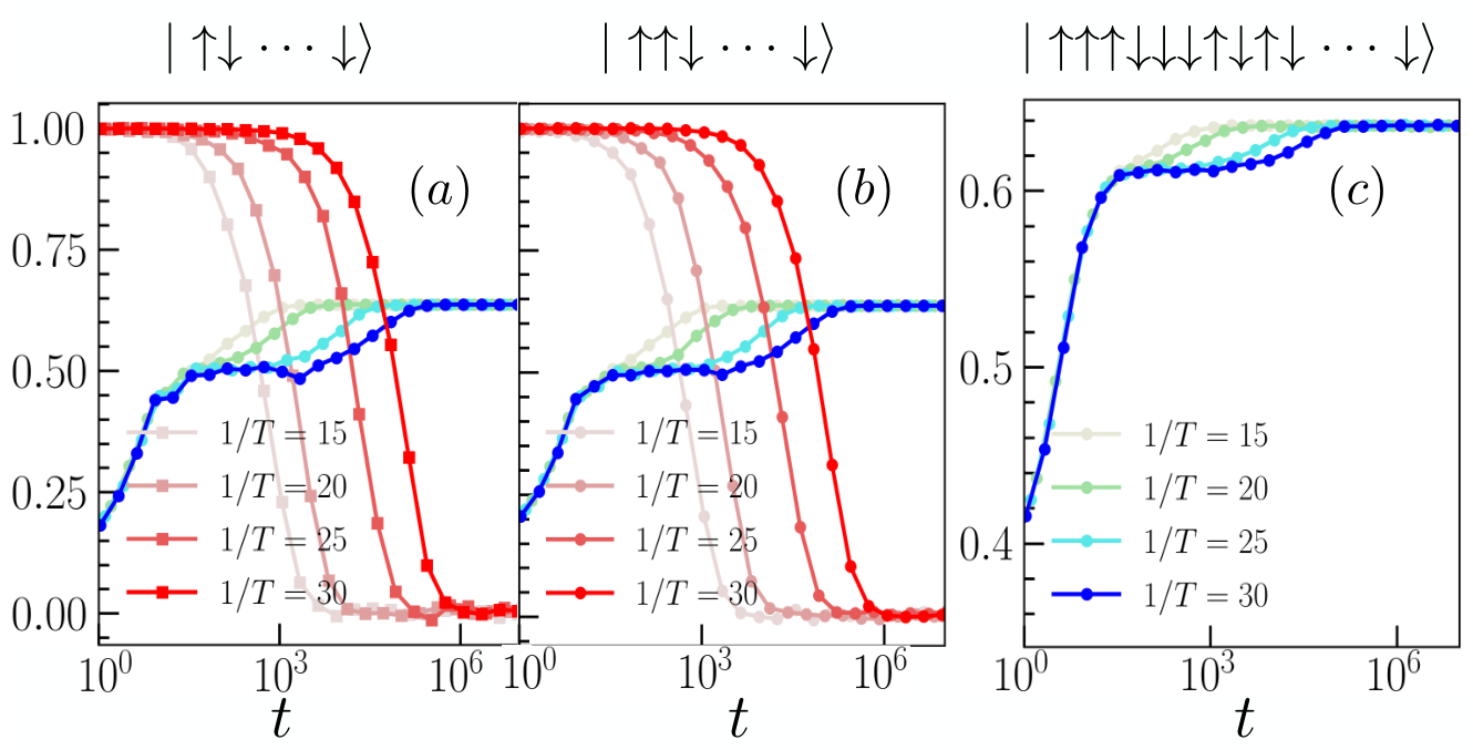

In the main content, the dynamics induced by Thue-Morse drives use all spins pointing down as the initial state. Here, we compare the dynamics for different initial states deviating from the fully polarized state with various numbers of domain walls. The results are plotted in Fig. 7 where we confirm the lack of energy absorption and a prethermal plateau as long as the initial state does not deviate too much from the ferromagnetic state.
The thermalization time are plotted in Fig. 8 on a Log scale, where the exponential dependence on can be clearly seen. The slope of the exponential fitting is insensitive to threshold values. As seen in the panel (c), different thresholds are applied to estimate while the slope of the fitting remain the same.
Appendix E Finite size effect
Here we compare the dynamics obtained for different system sizes. As seen in the right panel in Fig. 9 where the time is plotted on a log scale, one can hardly tell the differences between three results. In the left panel where the energy is plotted on a log scale, for the results show exponential decay and converge well for . In particular, at the mean energy used to determine thermalization time scaling in Fig. 3, , no finite size effect can be observed.

Finite size effect only becomes visible at late times not used for obtaining the scaling relation. There, the mean energy decreases notably for increasing system sizes, which is expected to be zero in the thermodynamic limit.
Appendix F Comparison between and -RMD for weak driving

Appendix G Prethermal DTC with imperfect rotation
Here we discuss the stability of the DTC with respect to imperfect spin flips used in Eq. 9 for a small . The magnetization dynamics for different perturbations are plotted in Fig. 11 (driving rate is ). The prethermal DTC remains stable for small perturbations, for instance . For , the amplitude of the period-doubling oscillation exhibits notable decay. For , no time-crystalline order exists and the oscillations around zero magnetization are induced by finite size effect.

It is not very surprising to see the phase is fragile to rotation imperfections as there is no mechanism to protect the system from thermalization. It will be interesting to investigate if disorder, long-range interactions or dissipation are capable of stabilizing the prethermal DTC further.