On regular and chaotic dynamics of a non- ${\cal{PT}}$ -symmetric Hamiltonian system of a coupled Duffing oscillator with balanced loss and gain

Pijush K. Ghosh Note: email: pijushkanti.ghosh@visva-bharati.ac.in Puspendu Roy Note: email:puspenduroy716@gmail.com

Department of Physics, Siksha-Bhavana,
Visva-Bharati University,
Santiniketan, PIN 731 235, India.

Abstract

A non- ${\cal{PT}}$ -symmetric Hamiltonian system of a Duffing oscillator coupled to an anti-damped oscillator with a variable angular frequency is shown to admit periodic solutions. The result implies that ${\cal{PT}}$ -symmetry of a Hamiltonian system with balanced loss and gain is not necessary in order to admit periodic solutions. The Hamiltonian describes a multistable dynamical system —three out of five equilibrium points are stable. The dynamics of the model is investigated in detail by using perturbative as well as numerical methods and shown to admit periodic solutions in some regions in the space of parameters. The phase transition from periodic to unbounded solution is to be understood without any reference to ${\cal{PT}}$ -symmetry. The numerical analysis reveals chaotic behaviour in the system beyond a critical value of the parameter that couples the Duffing oscillator to the anti-damped harmonic oscillator, thereby providing the first example of Hamiltonian chaos in a system with balanced loss and gain. The method of multiple time-scales is used for investigating the system perturbatively. The dynamics of the amplitude in the leading order of the perturbation is governed by an effective dimer model with balanced loss and gain that is non- ${\cal{PT}}$ -symmetric Hamiltonian system. The dimer model is solved exactly by using the Stokes variables and shown to admit periodic solutions in some regions of the parameter space.

Keywords: System with balanced loss and gain, Duffing oscillator, Chaos, Dimer Model

1 Introduction

The ${\cal{PT}}$ -symmetric classical Hamiltonian of coupled harmonic oscillators with balanced loss and gain admits periodic solution in the unbroken ${\cal{PT}}$ phase of the system[1]. The bounded solution becomes unbounded as a result of phase-transition from an unbroken to a broken ${\cal{PT}}$ phase. The change in the nature of solutions accompanied by the ${\cal{PT}}$ phase-transition has important physical consequences[2]. Further, the corresponding quantum system is well defined in appropriate Stokes wedges and admits bound states in the same unbroken ${\cal{PT}}$ phase[1]. This has lead to introduction of many ${\cal{PT}}$ -symmetric Hamiltonian systems with balanced loss and gain [3, 4, 5, 6, 7, 8, 9, 10]. The examples include many-particle systems[3, 7, 8, 9], systems with nonlinear interaction[4, 5, 6, 7, 8, 9], systems with space-dependent loss-gain terms[8], systems with Lorentz interaction[10] etc.. The important results which are common to all these models is that ${\cal{PT}}$ -symmetric Hamiltonian systems with balanced loss and gain may admit bounded and periodic solutions in some regions of the space of parameters. The bounded and unbounded solutions exist in the unbroken and broken ${\cal{PT}}$ -phases of the system, respectively. The corresponding quantum system admits bound states in well defined Stokes wedges. A few ${\cal{PT}}$ symmetric, but non-Hamiltonian classical systems with balanced loss and gain are also known to share the above properties[11, 12].

The investigations on classical Hamiltonian systems with balanced loss and gain are mostly restricted to ${\cal{PT}}$ symmetric models. One plausible reason is that ${\cal{PT}}$ -symmetric non-hermitian quantum systems admit entirely real spectra and unitary time-evolution in unbroken ${\cal{PT}}$ -phase[13]. The same result is valid for a non- ${\cal{PT}}$ -symmetric Hamiltonian provided it is pseudo-hermitian with respect to a positive-definite similarity operator[14] and/or admits an antilinear symmetry. A few examples of non- ${\cal{PT}}$ symmetric non-hermitian Hamiltonian admitting entirely real spectra and unitary time evolution may be found in the Refs.[14, 15, 16, 17, 18, 19, 20, 21]. It is known[7, 8] that systems involving a non-conventional ${\cal{T}}$ -symmetry also share the same properties. In classical mechanics, there is no notion of pseudo-hermiticity or anti-linear symmetry and the time-reversal symmetry is unique. Consequently, the criterion for a classical system with balanced loss and gain to admit periodic solution is solely based on ${\cal{PT}}$ -symmetry.

There are no compelling reasons to accept that only ${\cal{PT}}$ -symmetric classical Hamiltonian system with balanced loss and gain may admit periodic solutions. There should be enough provision for accommodating non- ${\cal{PT}}$ -symmetric classical Hamiltonian in the investigations on systems with balanced loss and gain, which upon quantization may lead to a pseudo-hermitian system and/or a Hamiltonian with an anti-linear symmetry different from the ${\cal{PT}}$ -symmetry. It may be noted here that the Hamiltonian formulation of generic systems with balanced loss and gain does not require any assumption on an underlying discrete or continuous symmetry[7, 8, 9, 10]. In particular, a Hamiltonian system in its standard formulation is necessarily non-dissipative, since the flow in the position-velocity state space preserves the volume. Thus, a system for which individual degrees of freedom are subjected to loss or gain is Hamiltonian only if the net loss-gain is zero[10]. This condition for the case of constant loss and gain essentially implies ${\cal{PT}}$ symmetry of the term $H_{0}=(P_{x}+\gamma y)(P_{y}-\gamma x)$ that appears in the Hamiltonian $H=H_{0}+V(x,y)$ , where $P_{x}$ and $P_{y}$ are canonical conjugate momenta corresponding to the coordinates $x$ and $y$ , respectively and $\gamma$ is the gain-loss parameter[1, 3, 4, 5, 6, 7, 8, 9, 10]. The Hamiltonian $H_{0}$ is not even required to be ${\cal{PT}}$ symmetric for the case of space-dependent loss-gain terms, i.e. $\gamma\equiv\gamma(x,y)$ [9, 10]. The most important point is that the potential $V(x,y)$ need not be ${\cal{PT}}$ -symmetric as far as the Hamiltonian formulation of systems with balanced loss and gain is considered[7, 8, 9, 10]. Further, there is no general result in a model independent way to suggest that ${\cal{PT}}$ -symmetry of $V(x,y)$ and hence, of $H$ is necessary in order to have periodic solutions. On the contrary, it is known that non-Hamiltonian dimer model without any ${\cal{PT}}$ symmetry due to imbalanced loss and gain admits stable nonlinear supermodes[22]. Similarly, within the mean field description of Bose-Einstein condensate, stationary ground state is obtained for non- ${\cal{PT}}$ -symmetric confining potential[23]. This raises the possibility that non- ${\cal{PT}}$ -symmetric Hamiltonian system with balanced loss and gain may admit periodic solutions with possible applications. It seems that non- ${\cal{PT}}$ symmetric Hamiltonian with balanced loss and gain has not been investigated so far for system with finite degrees of freedom.

The purpose of this article is to investigate regular as well as chaotic dynamics of a non- ${\cal{PT}}$ symmetric Hamiltonian system with balanced loss and gain. In particular, one of the objectives is to show that transition from periodic to unbounded solutions may be present in non- ${\cal{PT}}$ symmetric Hamiltonian systems with balanced loss and gain. The system is non- ${\cal{PT}}$ symmetric to start with and there is no question of attributing existence of these solutions to broken or unbroken ${\cal{PT}}$ -phases. Such transitions are quite common in generic dynamical systems with or without any specific symmetry and/or an underlying Hamiltonian structure. The inclusion of loss-gain terms with a Hamiltonian description of the system does not make much difference. The standard techniques may determine the region in the parameter space in which periodic solutions are obtained.

The second objective is to investigate chaotic dynamics of a non- ${\cal{PT}}$ symmetric Hamiltonian system with balanced loss and gain. It may be noted in this regard that chaos in ${\cal{PT}}$ symmetric systems has been studied earlier in different contexts[24, 25, 26]. Classical chaos has been studied in complex phase space for the kicked rotor and the double pendulum in Ref. [24], while the emphasis is on quantum kicked rotor and top in Ref. [25]. Chaotic behaviour in ${\cal{PT}}$ -symmetric models in optomechanics and magnomechanics has also been investigated[26]. No generic feature relating chaotic regime with that of broken or unbroken ${\cal{PT}}$ symmetry of the system is apparent from these investigations in a model independent way. Within this background, the requirement of ${\cal{PT}}$ symmetry appears to be too restrictive to explore chaotic behaviour in a larger class of systems with balanced loss and gain which may have possible technological applications. Thus, the emphasis is on non- ${\cal{PT}}$ -symmetric Hamiltonian system with balanced loss and gain.

The Duffing oscillator is a prototype example in the study of nonlinear dynamics[27, 28, 29]. It describes a damped harmonic oscillator with an additional cubic nonlinear term. The system admits different types of solutions in different regions of the space of parameters, including chaotic behaviour if the system is subjected to an external forcing. A Hamiltonian formulation for the Duffing oscillator is not known for non-vanishing damping term. However, following the methods described in Refs. [7, 9, 10], a Hamiltonian may be obtained for a system where the Duffing oscillator is coupled to an anti-damped harmonic oscillator in a nontrivial way. The coupling to the anti-damped oscillator effectively acts as a forcing term, thereby preparing the ground for investigating chaotic behaviour in the system. The dynamics of the Duffing oscillator completely decouples from the system in a particular limit, while the dynamics of the anti-damped oscillator is unidirectionally coupled to it. It should be emphasised here that even in this limit the anti-damped oscillator is not a time-reversed version of the Duffing oscillator. The system as a whole is non- ${\cal{PT}}$ -symmetric by construction. This is the Hamiltonian system of balanced loss and gain that will be studied in detail in this article for regular and chaotic dynamics.

The coupled Duffing oscillator with balanced loss and gain is analyzed by perturbative as well as numerical methods. The method of multiple scales[27, 30] is used to find approximate solutions in the leading order of perturbation parameter. The solutions are periodic in a region which is also obtained by linear stability analysis for the existence of periodic solution. It should be mentioned here that the linear stability analysis may or may not be valid for a Hamiltonian system with nonlinear interaction. However, periodic solutions are also obtained in the same region by numerically solving the equations of motions. There are unbounded solutions outside this region. This is one of the main results of this article —a non- ${\cal{PT}}$ -symmetric Hamiltonian system with balanced loss and gain admits periodic solution. The phase transition from periodic to unbounded solutions is specific to the model without any reference to ${\cal{PT}}$ -symmetry. The Hamiltonian is a multistable system —three out of the five equilibrium points are stable. The phase-space of the system has a rich structure. The bifurcation diagram of the system also shows chaotic behaviour beyond a critical value of the parameter that couples Duffing oscillator to the anti-damped oscillator. The role of this coupling term is similar to the forcing term of the standard forced Duffing oscillator, albeit in a nontrivial way. The chaotic behaviour of the system is confirmed independently by various methods. The chaotic behaviour in the coupled Duffing oscillator system with balanced loss and gain is another important result.

The present article also deals with a solvable non- ${\cal{PT}}$ -symmetric dimer Hamiltonian with balanced loss and gain which admits periodic solutions. The model of dimer arises as a byproduct of the perturbative analysis of the coupled Duffing oscillator model. In particular, different choices of the small parameters for implementing the perturbation scheme lead to different sets of equation for the time-evolution of the amplitude which may be interpreted as models of dimers. It is shown within this context that a model of non- ${\cal{PT}}$ -symmetric dimer with balanced loss and gain is exactly solvable and admits periodic solution in some regions of the parameter space. It seems that this is the first example of a non- ${\cal{PT}}$ -symmetric Hamiltonian dimer model with balanced loss and gain that admits periodic solution.

The plan of the article is the following. The model is introduced in Sec. 2. along with discussions on ${\cal{PT}}$ -symmetric limit of the system and linear stability analysis. A perturbative analysis of the system by using the method of multiple-scale analysis is presented in Sec. 3. The numerical result for the coupled Duffing-oscillator system is presented in Sec. 4. Non- ${\cal{PT}}$ -symmetric Hamiltonian of a dimer with balanced loss and gain is presented in Sec. 5. Finally, discussions on the results are presented in Sec. 6. Perturbative analysis of the model by treating the gain-loss coefficient and the coupling constant of the nonlinear interaction as small parameters are presented in Appendix-I in Sec. 8.

2 The Model

The system described by the equations of motion,

	$\displaystyle\ddot{x}+2\gamma\dot{x}+\omega^{2}x+\beta_{1}y+gx^{3}=0,$
	$\displaystyle\ddot{y}-2\gamma\dot{y}+\omega^{2}y+\beta_{2}x+3gx^{2}y=0,$		(1)

is a model of coupled oscillators with nonlinear interaction and subjected to gain and loss. The parameters $\gamma,\omega$ and $g$ correspond to the loss-gain strength, angular frequency of the harmonic trap and the nonlinear coupling strength, respectively. The linear coupling between the $x$ and $y$ degrees of freedom is denoted by the real constants $\beta_{1}$ and $\beta_{2}$ . The linear coupling is asymmetric for $\beta_{1}\neq\beta_{2}$ . The above equation describes a system of balanced loss and gain in the sense that the flow in the position-velocity state space preserves the volume, although individual degrees of freedom are subjected to gain or loss. The system admits a Hamiltonian,

\displaystyle H=P_{x}P_{y}+\gamma\left(yP_{y}-xP_{x}\right)+\left(\omega^{2}-{\gamma^{2}}\right)xy+\frac{1}{2}\left(\beta_{2}x^{2}+\beta_{1}y^{2}\right)+gx^{3}y,\

(2)

where $P_{x}$ and $P_{y}$ are canonical momenta,

\displaystyle P_{x}=\dot{y}-\gamma y,\ \ P_{y}=\dot{x}+\gamma x.

(3)

The equations of motion (1) may be obtained from $H$ . The Hamiltonian $H$ reduces to a system of coupled harmonic oscillators with balanced loss and gain for $g=0$ and $\beta_{1}=\beta_{2}$ which admits periodic solutions[1] in the unbroken ${\cal{PT}}$ phase of the system. Generalisations of the coupled oscillators model of Ref. [1] have been considered earlier by including cubic nonlinearity and preserving the ${\cal{PT}}$ -symmetry[4, 6] of the system. As will be shown below, the Hamiltonian $H$ for $g\neq 0$ is not ${\cal{PT}}$ -symmetric and there is no question of a broken or unbroken ${\cal{PT}}$ phases of it. However, the system admits periodic solutions in restricted region of the parameter space. This is a major difference from previous investigations on models of coupled oscillators with balanced loss and gain, where the periodic solutions are attributed to unbroken ${\cal{PT}}$ -phases.

The system described by Eqs. (1,2) has an interesting limit $\beta_{1}=0$ for which the $x$ degree of freedom completely decouples from the $y$ degree of freedom and describes an unforced Duffing oscillator. The Hamiltonian $H$ for $\beta_{1}=0$ corresponds to the Hamiltonian of Duffing oscillator in an ambient space of two dimensions, where the auxiliary system is described in terms of $y$ degree of freedom and corresponds to a forced anti-damped harmonic oscillator with time-dependent frequency. The time-dependence of the frequency $\omega^{2}+3gx^{2}$ is implicit via its dependence on $x$ . Similarly, the time-dependence of the forcing term $\beta_{2}x$ is determined by the solutions of the unforced Duffing oscillator. This paves the way for using well known tools and techniques associated with a Hamiltonian system to analyse Duffing oscillator analytically. For example, methods of canonical perturbation theory, canonical quantization, integrability, Hamiltonian chaos etc. can be used for investigating Duffing oscillator. The present article deals with only the dynamical behaviour of the system for $\beta_{1}\neq 0$ .

The distinction between ambient and target spaces ceases to exist for $\beta_{1}\neq 0$ and $H$ constitutes a new class of system with balanced loss and gain. The system governed by $H$ with generic values of the parameters may be interpreted as describing a non-standard forced Duffing oscillator with the identification of $\beta_{1}y$ in the first equation of (1) as the ‘forcing term’. The forcing term in case of standard Duffing oscillator can be chosen. However, for the case of non-standard Duffing oscillator it is determined in a nontrivial way from the second equation of (1) which is also coupled to the first equation. Eq. (1) can be also interpreted as two coupled undamped, unforced Duffing oscillators with velocity as well as space mediated coupling terms. In particular, Eq. (1) can be rewritten as,

	$\displaystyle\ddot{u}+\Omega_{+}u+gu^{3}+\left\{2\gamma\dot{v}+\frac{\beta_{2}-\beta_{1}}{2}v-\frac{g}{2}v\left(v^{2}-3u^{2}\right)\right\}=0,$
	$\displaystyle\ddot{v}+\Omega_{-}v+gv^{3}+\left\{2\gamma\dot{u}-\frac{\beta_{2}-\beta_{1}}{2}u-\frac{g}{2}u\left(u^{2}-3v^{2}\right)\right\}=0,\ \Omega_{\pm}\equiv\omega^{2}\pm\frac{\beta_{1}+\beta_{2}}{2}$		(4)

in the rotated co-ordinate system $(u,v)$ defined by the relations,

\displaystyle u=\frac{x+y}{\sqrt{2}},\ v=\frac{x-y}{\sqrt{2}},\ \ P_{u}=\frac{P_{x}+P_{y}}{\sqrt{2}},\ P_{v}=\frac{P_{x}-P_{y}}{\sqrt{2}}.

(5)

In general, the coefficients $\Omega_{\pm}$ of the harmonic terms are different and becomes identical, $\Omega_{+}=\Omega_{-}=\omega^{2}$ for $\beta_{1}=-\beta_{2}$ . Moreover, either $\Omega_{+}$ or $\Omega_{-}$ can be chosen to be zero for $\omega^{2}=-\frac{\beta_{1}+\beta_{2}}{2}$ or $\omega^{2}=\frac{\beta_{1}+\beta_{2}}{2}$ , respectively. The loss and gain terms are hidden in the $(u,v)$ co-ordinate system and give rise to velocity mediated coupling between the two Duffing oscillators. The space mediated coupling between the oscillators comprise of linear as well as nonlinear terms. The linear term vanishes for $\beta_{1}=\beta_{2}$ and in the limit of vanishing strength of the nonlinear coupling between the Duffing oscillators, i.e. $g\rightarrow 0$ , the system describes a linear system that has been studied earlier[1]. The Hamiltonian in the $(u,v)$ co-ordinate system has the following form:

\displaystyle H_{u}=\frac{1}{2}\left(P_{u}-\gamma v\right)^{2}-\frac{1}{2}\left(P_{v}+\gamma u\right)^{2}+\frac{\Omega_{+}}{2}u^{2}-\frac{\Omega_{-}}{2}v^{2}+\frac{g}{4}\left(u^{4}-v^{4}\right)+\frac{uv}{2}\left[\beta_{2}-\beta_{1}+g(u^{2}-v^{2})\right].

(6)

It is expected that some of the behaviours of the standard forced Duffing oscillator will persist for the model under investigation. The $(u,v)$ co-ordinates are used solely for the purpose of interpreting the model as coupled Duffing oscillators. The rest of the discussions in this article will be based on $(x,y)$ co-ordinates.

2.1 Scale-transformation

The following transformations are employed,

\displaystyle t\rightarrow\omega^{-1}t,\ x\rightarrow{|\beta_{2}|}^{-\frac{1}{2}}x,\ y\rightarrow{|\beta_{1}|}^{-\frac{1}{2}}y,\ \beta_{1}\neq 0,\beta_{2}\neq 0,

(7)

in order to fix the independent scales in the system. This allows a reduction in total number of independent parameters which is convenient for analyzing the system. The model can be described in terms of three independent parameters $\Gamma,\beta$ and $\alpha$ defined as,

\displaystyle\Gamma=\frac{\gamma}{\omega},\beta=\frac{\sqrt{{|{\beta_{1}}|}{|{\beta_{2}}|}}}{\omega^{2}},\alpha=\frac{g}{{|\beta_{2}|}\omega^{2}},

(8)

and the equations of motion have the following expressions:

	$\displaystyle\ddot{x}+2\Gamma\dot{x}+x+\sgn(\beta_{1})\ \beta y+\alpha x^{3}=0,$
	$\displaystyle\ddot{y}-2\Gamma\dot{y}+y+\sgn(\beta_{2})\ \beta x+3\alpha x^{2}y=0.$		(9)

The sign-function $\sgn(x)$ is defined for $x\neq 0$ as $\sgn(x)=\frac{x}{|x|},\ x\in\mathbb{R}$ . The limit to the linear system $g\rightarrow 0$ now corresponds to $\alpha\rightarrow 0$ . The linear coupling between the two oscillator modes with the strength $\beta$ comprises of two distinct cases:

•

Linear Symmetric Coupling(LSC): The signs of the linear coupling terms in Eq. (9) are same for this case and it occurs either for (a) $\beta_{1},\beta_{2}>0$ or (b) $\beta_{1},\beta_{2}<0$ . It may be noted that the linear coupling terms $(\ \sgn(\beta_{1})\ \beta y,\ \sgn(\beta_{2})\ \beta x)$ appearing in Eq. (9) reduce to $(\beta y,\beta x)$ and $(-\beta y,-\beta x)$ for the case (a) and the case (b), respectively. These two cases correspond to positive and negative linear coupling strengths, since $\beta>0$ . It is apparent that Eq. (9) for the case (a) is related to the same equation with case (b) via the transformation $\beta\rightarrow-\beta$ . Thus, it is suffice to consider the positive LSC only from which the results for the negative LSC may be obtained by taking $\beta\rightarrow-\beta$ . The effect of the asymmetric linear coupling between the oscillators in Eq. (1) is encoded in the nonlinear coupling $\alpha$ through its dependence on ${|\beta_{2}|}$ .
•

Linear Anti-symmetric Coupling(LAC): A relative sign difference between the linear coupling terms in Eq. (9) is termed as LAC which may be obtained either for $\beta_{1}>0,\beta_{2}<0$ or $\beta_{1}<0,\beta_{2}>0$ . It can be shown that the linear model, i.e. $\alpha=0$ , for the anti-symmetric coupling does not admit any periodic solutions. Numerical analysis for the nonlinear model in a limited region of the parameter space indicates that it may not admit periodic and/or stable solutions. An exhaustive numerical analysis is required to ascertain this which is beyond the scope of this article and LAC will not be pursued further for perturbative and numerical analysis.

The scale transformation (7) implies,

P_{x}\rightarrow\frac{\omega}{\sqrt{\beta_{1}}}\tilde{P}_{x},P_{y}\rightarrow\frac{\omega}{\sqrt{\beta_{2}}}\tilde{P}_{y},H\rightarrow\beta^{-1}\tilde{H},

(10)

where $\tilde{P}_{x}=\dot{y}-\Gamma y,\ \tilde{P}_{y}=\dot{x}+\Gamma x$ and

\displaystyle\tilde{H}=\tilde{P}_{x}\tilde{P_{y}}+\Gamma\left(y\tilde{P}_{y}-x\tilde{P}_{x}\right)+\left(1-\Gamma^{2}\right)xy+\frac{\beta}{2}\left[\sgn(\beta_{2})\ x^{2}+\sgn(\beta_{1})\ y^{2}\right]+\alpha x^{3}y.

(11)

The Hamiltonian $\tilde{H}$ and the equations of motion in (9) will be considered for further analysis and the results in terms of the original variables may be obtained by inverse scale transformations. Defining generalized momenta $\Pi_{x}=\tilde{P}_{x}+\Gamma y,\Pi_{y}=\tilde{P}_{y}-\Gamma x$ , the Hamiltonian can be rewritten as,

\displaystyle\tilde{H}=\Pi_{x}\Pi_{y}+V(x,y),\ \ V(x,y)=xy+\frac{\beta}{2}\left[\sgn(\beta_{2})\ x^{2}+\sgn(\beta_{1})\ y^{2}\right]+\alpha x^{3}y.

(12)

The Hamiltonian $\tilde{H}$ or equivalently the energy $E=\dot{x}\dot{y}+V(x,y)$ is a constant of motion, but neither semi-positive definite nor bounded from below. The energy may be bounded from below for specific orbits in the phase-space to be determined from the equations of motion.

2.2 ${\cal{PT}}$ -Symmetry

The Hamiltonian may be interpreted as a two dimensional system with a single particle or a system of two particles in one dimension. The Hamiltonian $H$ or $\tilde{H}$ is not ${\cal{PT}}$ -symmetric for either of the cases. For example, with the interpretation of $\tilde{H}$ describing a system of two particles in one dimension, the parity( ${\cal{P}}_{1})$ and ${\cal{T}}$ symmetry are defined as,

	$\displaystyle{\cal{T}}:t\rightarrow-t,\ \tilde{P}_{x}\rightarrow-\tilde{P}_{x},\ \tilde{P}_{y}\rightarrow-\tilde{P}_{y}$
	$\displaystyle{\cal{P}}_{1}:\ x\rightarrow-x,\ y\rightarrow-y,\tilde{P}_{x}\rightarrow-\tilde{P}_{x},\ \tilde{P}_{y}\rightarrow-\tilde{P}_{y}.$		(13)

The term linear in $\Gamma$ is not invariant under ${\cal{P}}_{1}{\cal{T}}$ symmetry. Similarly, the system is not invariant under ${\cal{PT}}$ symmetry even if the parity ( ${\cal{P}}$ ) transformation in two dimensions is considered in its most general form:

\displaystyle{\cal{P}}:\begin{pmatrix}{x}\\ {y}\end{pmatrix}\rightarrow\begin{pmatrix}{x^{\prime}}\\ y^{\prime}\end{pmatrix}=\begin{pmatrix}{x\cos\theta+y\sin\theta}\\ {x\sin\theta-y\cos\theta}\end{pmatrix},\ \begin{pmatrix}{\tilde{P}_{x}}\\ {\tilde{P}_{y}}\end{pmatrix}\rightarrow\begin{pmatrix}{\tilde{P}_{x}^{\prime}}\\ \tilde{P}_{y}^{\prime}\end{pmatrix}=\begin{pmatrix}{\tilde{P}_{x}\cos\theta+\tilde{P}_{y}\sin\theta}\\ {\tilde{P}_{x}\sin\theta-\tilde{P}_{y}\cos\theta}\end{pmatrix}

(14)

where $\theta\in(0,2\pi)$ . The first term in $\tilde{H}$ is invariant under ${\cal{T}}$ , while it is invariant under ${\cal{P}}$ only for two distinct values of $\theta$ , namely, $\theta=\frac{\pi}{2},\frac{3\pi}{2}$ . It may be noted that $\theta=\frac{\pi}{2}$ corresponds to ${\cal{P}}:(x,y)\rightarrow(y,x),(\tilde{P}_{x},\tilde{P}_{y})\rightarrow(\tilde{P}_{y},\tilde{P}_{x})$ , while ${\cal{P}}:(x,y)\rightarrow(-y,-x),(\tilde{P}_{x},\tilde{P}_{y})\rightarrow(-\tilde{P}_{y},-\tilde{P}_{x})$ for $\theta=\frac{3\pi}{2}$ . The second, third and the fourth terms of $\tilde{H}$ in Eq. (11) are invariant under ${\cal{PT}}$ symmetry for these two values of $\theta$ and LSC. However, the nonlinear coupling term breaks ${\cal{PT}}$ symmetry for $\alpha\neq 0$ . It may be noted that $H$ in Eq. (2) is not invariant under ${\cal{PT}}$ symmetry for $\beta_{1}\neq\beta_{2}$ even for vanishing nonlinear coupling, i.e. $g=0$ . The scale transformation plays an important role for showing implicit ${\cal{PT}}$ invariance of $H$ with $g=0$ and LSC. The fourth term of $\tilde{H}$ breaks ${\cal{PT}}$ symmetry for the LAC and is related to the result that $H$ is not ${\cal{PT}}$ symmetric for $\beta_{1}\neq\beta_{2}$ . A non-vanishing nonlinear interaction necessarily breaks ${\cal{PT}}$ invariance for $H$ and $\tilde{H}$ irrespective of LSC or LAC.

2.3 Stability Analysis

The Hamilton’s equations of motion,

	$\displaystyle\dot{x}=\tilde{P}_{y}-\Gamma x,\ \ \dot{y}=\tilde{P}_{x}+\Gamma y,$
	$\displaystyle\dot{\tilde{P}}_{x}=-\beta x+\Gamma\tilde{P}_{x}+(\Gamma^{2}-1)y-3\alpha x^{2}y,$
	$\displaystyle\dot{\tilde{P}}_{y}=-\beta y-\Gamma\tilde{P}_{y}+(\Gamma^{2}-1)x-\alpha x^{3},$		(15)

are equivalent to the coupled second order equations (9) with positive LSC. Results for negative LSC may be obtained by taking $\beta\rightarrow-\beta$ . The equilibrium points and their stability may be analyzed by employing standard techniques. In particular, the equilibrium points are determined by the solutions of the algebraic equations obtained by putting the right hand side of Eq. (15) equal to zero. According to the Dirichlet theorem[31], an equilibrium point is stable provided the second variation of the Hamiltonian is definite at that point. This is neither a necessary condition nor the converse is true. If the application of the Dirichlet theorem leads to inconclusive results, a linear stability analysis may be performed, which is an approximate method. The method involves the study of time-evolution of small fluctuations around an equilibrium point by keeping only linear terms. The quadratic and higher order fluctuations are neglected due to its smallness. The resulting linear system of coupled differential equations can be solved to study the time-evolution of the fluctuations. A detailed classification of equilibrium points based on the time-evolution of small fluctuation may be found in any standard reference on nonlinear differential equation, including the Refs. [27, 32]. A Hamiltonian system admits either center i.e. closed orbit in the phase-space surrounding an equilibrium point or hyperbolic point signalling instability[32]. The stable equilibrium point of a Hamiltonian system necessarily corresponds to a center. It should be noted that a center is not asymptotically stable.

2.3.1 Equilibrium Points and the Dirichlet Theorem

The system admits five equilibrium points $P_{0},P_{1}^{\pm},P_{2}^{\pm}$ in the phase-space $(x,y,\tilde{P}_{x},\tilde{P}_{y})$ of the system, which are determined by the solutions of the algebraic equations obtained by putting the right hand side of Eq. (15) equal to zero. The equilibrium points are,

P_{0}=(0,0,0,0),P_{1}^{\pm}=(\pm\delta_{+},\pm\eta_{+},\mp\Gamma\eta_{+},\pm\Gamma\delta_{+}),P_{2}^{\pm}=(\pm\delta_{-},\pm\eta_{-},\mp\Gamma\eta_{-},\pm\Gamma\delta_{-}),

(16)

where $\delta_{\pm}$ and $\eta_{\pm}$ are defined as follows:

\displaystyle\delta_{\pm}=\frac{1}{\sqrt{3\alpha}}\left[-2\pm\sqrt{1+3\beta^{2}}\right]^{\frac{1}{2}},\ \ \eta_{\pm}=-\frac{\delta_{\pm}}{3\beta}\left[1\pm\sqrt{1+3\beta^{2}}\right].

(17)

The points $P_{1}^{\pm}$ are related to each other through the relation $P_{1}^{\pm}=-P_{1}^{\mp}$ . The projections of the points $P_{1}^{\pm}$ on the ‘ $x-y$ ’-plane are related through a rotation by an angle $\pi$ . This is a manifestation of the fact that Eq. (9) remains invariant under the transformation $x\rightarrow-x,y\rightarrow-y$ for fixed $\alpha,\beta,\Gamma$ . Under the same transformation $\tilde{P}_{x}\rightarrow-\tilde{P}_{x},\tilde{P}_{y}\rightarrow-\tilde{P}_{y}$ , and Eq. (15) remains invariant under $(x,y,\tilde{P}_{x},\tilde{P}_{y})\rightarrow(-x,-y,-\tilde{P}_{x},-\tilde{P}_{y})$ . The relation $P_{2}^{\pm}=-P_{2}^{\mp}$ may be explained in the same way.

The equilibrium point $P_{0}$ exists all over the parameter space, while all other points exist in restricted regions in the parameter space. In particular,

•

${\bf\alpha>0}$ : $P_{0},P_{1}^{\pm}$ are equilibrium points for $\beta^{2}>1$ , while $P_{0}$ is the only equilibrium point for $0<\beta^{2}\leq 1$ . Points $P_{2}^{\pm}$ are non-existent, since $\delta_{\pm}$ and $\eta_{\pm}$ are purely imaginary.
•

${\bf\alpha<0}$ : $P_{0},P_{1}^{\pm},P_{2}^{\pm}$ are equilibrium points for $0<\beta^{2}<1$ , while $P_{0},P_{2}^{\pm}$ are equilibrium points for $\beta^{2}\geq 1$ .
•

${\bf\alpha=0}$ : Only $P_{0}$ is the equilibrium point.

The critical points of the Hamiltonian $\tilde{H}$ are also located at $P_{0},P_{1}^{\pm},P_{2}^{\pm}$ , since the equilibrium points correspond to the solutions of the equations $\tilde{H}_{Z}\equiv\frac{\partial\tilde{H}}{\partial Z}=0,Z\equiv(x,y,\tilde{P}_{x},\tilde{P}_{y})$ . However, the Hessian $\tilde{H}_{ZZ}$ of $H$ is not definite at these equilibrium points in any region of the parameter-space. For example, the four eigenvalues of $\tilde{H}_{ZZ}$ at $P_{0}$ are determined as,

\frac{1}{2}\left[\beta+\Gamma^{2}\pm\left\{4(1-\beta)+(\beta+\Gamma^{2})^{2}\right\}^{\frac{1}{2}}\right],\ \frac{1}{2}\left[\beta-\Gamma^{2}\pm\left\{4(1+\beta)+(\beta-\Gamma^{2})^{2}\right\}^{\frac{1}{2}}\right].

(18)

The spectrum always consists of positive as well negative eigenvalues for fixed $\Gamma$ and $\beta$ — all the four eigenvalues are neither semi-positive definite nor negative-definite simultaneously. Thus, the second variation of $\tilde{H}$ is not definite at $P_{0}$ and no conclusion can be drawn about its stability by using the Dirichlet theorem[31]. A similar analytical treatment for the points $P_{1}^{\pm}$ and $P_{2}^{\pm}$ become cumbersome. However, numerical investigations for some chosen values of the parameters indicate that the eigenvalues of the Hessian of $H$ for none of the points are definite.

2.3.2 Linear Stability Analysis

In absence of any definite results on the stability of equilibrium points by the use of Dirichlet theorem, a linear stability analysis may be performed. Considering small fluctuations around an equilibrium point $(x_{0},y_{0},\tilde{P}_{x_{0}},\tilde{P}_{y_{0}})$ in the phase space as $(x=x_{0}+\xi_{1},y=y_{0}+\xi_{2},\tilde{P}_{x}=\tilde{P}_{x_{0}}+\xi_{3},\tilde{P}_{y}=\tilde{P}_{y_{0}}+\xi_{4})$ and keeping only the terms linear in $\xi_{i}$ in Eq. (15), the following equation is obtained,

\displaystyle\dot{\xi}=M\xi,\ \ M=\begin{pmatrix}{-\Gamma}&&{0}&&{0}&&{1}\\ {0}&&{\Gamma}&&{1}&&{0}\\ -(\beta+6\alpha x_{0}y_{0})&&\Gamma^{2}-1-3\alpha x_{0}^{2}&&\Gamma&&0\\ \Gamma^{2}-1-3\alpha x_{0}^{2}&&-\beta&&0&&-\Gamma\end{pmatrix},

(19)

where $\xi=(\xi_{1},\xi_{2},\xi_{3},\xi_{4})^{T}$ and $A^{T}$ denotes transpose of $A$ . The values of $x_{0},y_{0},\tilde{P}_{x_{0}},\tilde{P}_{y_{0}}$ differ for each equilibrium point and may be substituted at an appropriate step of the stability analysis. The characteristic equation of the matrix $M$ and its solutions $\pm i\lambda_{j},j=1,2$ are determined as,

	$\displaystyle\lambda^{4}+2\left(1+3\alpha x_{0}^{2}-2\Gamma^{2}\right)\lambda^{2}+(1+3\alpha x_{0}^{2})^{2}-\beta^{2}-6\alpha\beta x_{0}y_{0}=0,$
	$\displaystyle\lambda_{j}=\left[1-2\Gamma^{2}+3\alpha x_{0}^{2}-(-1)^{j+1}\sqrt{\beta^{2}+4\Gamma^{4}-4\Gamma^{2}(1+3\alpha x_{0}^{2})+6\alpha\beta x_{0}y_{0}}\right]^{\frac{1}{2}}.$		(20)

The stable solutions are obtained in different regions of the parameter space for which $\lambda_{j}\in\mathbb{Re}\ \forall\ j$ . Each equilibrium point is analyzed separately for its stability.

•

Point $P_{0}$ : The equilibrium point $P_{0}$ corresponds to $x_{0}=y_{0}=0$ and is stable in a region of parameter-space defined by the conditions,

$\displaystyle-\frac{1}{\sqrt{2}}<\Gamma<\frac{1}{\sqrt{2}},\ \ 4\Gamma^{2}\left(1-\Gamma^{2}\right)<\beta^{2}<1.$ (21)

These inequalities are equivalent to the following conditions:

$\displaystyle\frac{1}{2}<\beta^{2}<1,\ \ -\Gamma_{0}<\Gamma<\Gamma_{0},\ \Gamma_{0}\equiv\frac{1}{\sqrt{2}}\sqrt{1-\sqrt{1-\beta^{2}}}.$ (22)

The point $P_{0}$ is a stable equilibrium point for any $\alpha$ and restricted values of $\beta$ and $\Gamma$ specified by the condition (21). The system with $\alpha=0$ corresponds to the coupled oscillator model of Ref. [1] and appears as linear part of the coupled Duffing oscillators models[4, 11]. The stable equilibrium point $P_{0}$ with the same stability condition has been found for all these models.

•

Point $P_{1}^{\pm}$ : It may be noted that $x_{0}^{2}=\delta_{+}^{2}$ and $x_{0}y_{0}=\delta_{+}\eta_{+}$ for both the points $P_{1}^{\pm}$ . The eigenvalues $\lambda_{j}$ are same for both the points $P_{1}^{\pm}$ and a simplified expression may be obtained as,

\displaystyle\lambda_{j}^{2}=-1-2\Gamma^{2}+S-\frac{(-1)^{j+1}}{\sqrt{3}}\sqrt{3-S^{2}+12\Gamma^{4}+12\Gamma^{2}-S(12\Gamma^{2}-2)},\ \ \ j=1,2,

(23)

where $S=\sqrt{1+3\beta^{2}}$ . Stable solutions for these two points exist in the same region in parameter space:

\displaystyle\beta^{2}>1,\ \ \Gamma^{2}\leq\frac{\sqrt{2}-1}{2}.

(24)

The equilibrium points $P_{1}^{\pm}$ exist for $\alpha>0,\beta^{2}>1$ and $\alpha<0,0<\beta^{2}<1$ . Thus, $P_{1}^{\pm}$ are stable for $\alpha>0$ and unstable for $\alpha<0$ . The stable equilibrium points $P_{1}^{\pm}$ are specific to the nonlinear interaction of the model.

•

Point $P_{2}^{\pm}$ : It may be noted that $x_{0}^{2}=\delta_{-}^{2}$ and $x_{0}y_{0}=\delta_{-}\eta_{-}$ for both the points $P_{2}^{\pm}$ . Stable solutions for these two points do not exist anywhere in parameter space, since

\displaystyle-\lambda_{j}^{2}=1+2\Gamma^{2}+S+\frac{(-1)^{j+1}}{\sqrt{3}}\sqrt{3-S^{2}+12\Gamma^{4}+12\Gamma^{2}+S(12\Gamma^{2}-2)},\ \ \ j=1,2,

(25)

implies that at least one eigenvalue has a non-vanishing imaginary part.

The Hamiltonian describes a multistable system — the points $P_{0}$ and $P_{1}^{\pm}$ are stable for $\alpha>0$ with the condition (21) for $P_{0}$ and the condition (24) for $P_{1}^{\pm}$ . For $\alpha<0$ , only $P_{0}$ is the stable point. No multistable system within the context of systems with balanced loss and gain has been reported earlier.

All the stable equilibrium points are ‘center’[27, 32], i.e. all the eigenvalues of $M$ are purely imaginary. It should be kept in mind that the linear stability analysis may or may not hold for center and/or a Hamiltonian system when the effect of the nonlinear interaction is considered[32]. The result is only indicative for scanning a large parameter space in order to find bounded solution by using perturbative and/or numerical methods. It will be seen that there are bounded solution for the model under investigation whenever conditions (21) or (24) are satisfied as well as in other regions of the parameter space for which no information can be gained from the linear stability analysis.

3 Perturbative Solution

Introducing the following matrices,

\displaystyle X=\begin{pmatrix}x\\ y\end{pmatrix},\ \ P=\begin{pmatrix}1&&\beta\\ \beta&&1\end{pmatrix},\ \ \tilde{V}(x,y)=\begin{pmatrix}x^{3}\\ 3x^{2}y\end{pmatrix}

(26)

and denoting the Pauli matrices as $\sigma_{a},a=1,2,3$ with $\sigma_{3}$ taken to be diagonal, Eq. (9) with positive LSC can be rewritten as,

\displaystyle\ddot{X}+2\Gamma\sigma_{3}\dot{X}+PX+\alpha\tilde{V}(x)=0.

(27)

Results for negative LSC may be obtained by taking $\beta\rightarrow-\beta$ . The system of coupled linear oscillators with balanced loss-gain corresponds to $\alpha=0$ and is exactly solvable. The nonlinear interaction is treated as perturbation for $\alpha\ll 1$ . The standard perturbation theory fails due to the appearance of secular terms, which are unbounded in time and lead to divergences in the long-time behaviour of the solutions. One of the possible remedies is to use the method of multiple time-scales[30] in which many time-variables are introduced temporarily by multiplying the original time $t$ with different powers of $\alpha$ . In particular, the coordinates are expressed in powers of the small parameter $\alpha$ and multiple time-scales are introduced as follows,

\displaystyle T_{n}=\alpha^{n}t,\ \ X=\sum_{n=0}^{\infty}\alpha^{n}X^{(n)}(T_{0},T_{1},\dots),\ \ X^{(n)}=\begin{pmatrix}x_{n}\\ y_{n}\end{pmatrix}.

(28)

This introduces slow and fast time scales in the system. For example, $T_{n+1}$ is always slower than $T_{n}$ , since $\alpha\ll 1$ . Using Eq. (28) in Eq. (27) and equating the terms with the same coefficient $\alpha^{n}$ to zero, the following equations up to $O(\alpha)$ are obtained as follows:

	$\displaystyle{\cal{O}}(\alpha^{0}):\frac{\partial^{2}X^{(0)}}{\partial T_{0}^{2}}+2\Gamma\sigma_{3}\frac{\partial X^{(0)}}{\partial T_{0}}+PX^{(0)}=0,$		(29)
	$\displaystyle{\cal{O}}(\alpha):\frac{\partial^{2}X^{(1)}}{\partial T_{0}^{2}}+2\Gamma\sigma_{3}\frac{\partial X^{(1)}}{\partial T_{0}}+PX^{(1)}+2\frac{\partial^{2}X^{(0)}}{\partial T_{0}\partial T_{1}}+2\Gamma\sigma_{3}\frac{\partial X^{(0)}}{\partial T_{1}}+\begin{pmatrix}x_{0}^{3}\\ 3x_{0}^{2}y_{0}\end{pmatrix}=0.$		(30)

The unperturbed Eq. (29) has the solution,

\displaystyle X^{(0)}=A_{0}\ e^{-i{\lambda_{1}}T_{0}}\begin{pmatrix}1\\ \eta_{1}\end{pmatrix}+B_{0}\ e^{-i{\lambda_{2}}T_{0}}\begin{pmatrix}1\\ \eta_{2}\end{pmatrix}+c.c.,\ \ \eta_{j}=\frac{1}{\beta}\left(\lambda_{j}^{2}+2i\Gamma\lambda_{j}-1\right),

(31)

where $A_{0}\equiv A_{0}(T_{1},T_{2},\dots)$ and $B_{0}\equiv B_{0}(T_{1},T_{2},\dots)$ are independent of $T_{0}$ , but, depends on slower time scales $T_{1},T_{2},\dots$ and c.c. denotes complex conjugate. The expressions for the eigenvalues $\lambda_{1},\lambda_{2}$ are given by Eq. (20) with $x_{0}=0,y_{0}=0$ , i.e. eigenvalues associated with the stability of the point $P_{0}$ . In order to find dependence of $A_{0}$ and $B_{0}$ on $T_{1}$ , Eq. (30) is to be solved by eliminating secular terms.

The ${\cal{O}}(\alpha)$ Eq. (30) is a linear inhomogeneous equation and the complementary solution is obtained by replacing $(A_{0},B_{0})\rightarrow(A_{1},B_{1})$ in Eq. (31) describing $X^{(0)}$ , where $A_{1}\equiv A_{1}(T_{1},T_{2},\dots)$ and $B_{1}\equiv B_{1}(T_{1},T_{2},\dots)$ are independent of $T_{0}$ . The particular solution $Y^{(1)}$ is determined from the equation,

\displaystyle\frac{\partial^{2}Y^{(1)}}{\partial T_{0}^{2}}+2\Gamma\sigma_{3}\frac{\partial Y^{(1)}}{\partial T_{0}}+PY^{(1)}=B,

(32)

where $-B$ is the inhomogeneous part of Eq. (30). With the introduction of two complex parameters $z_{j}=\Gamma+i\lambda_{j}$ and substituting the solution $X^{(0)}$ , $B$ has the following expression:

$\displaystyle-B$	$\displaystyle=$	$\displaystyle e^{-i{\lambda_{1}}T_{0}}\begin{pmatrix}2z_{1}^{}\frac{\partial A_{0}}{\partial T_{1}}+3A_{0}\left({\|A_{0}\|}^{2}+2{\|B_{0}\|}^{2}\right)\\ -2\eta_{1}z_{1}\frac{\partial A_{0}}{\partial T_{1}}+3A_{0}\left\{{\|A_{0}\|}^{2}\left(2\eta_{1}+\eta_{1}^{}\right)+2{\|B_{0}\|}^{2}\left(\eta_{1}+\eta_{2}+\eta_{2}^{*}\right)\right\}\end{pmatrix}$	(33)
	$\displaystyle+$	$\displaystyle e^{-i{\lambda_{2}}T_{0}}\begin{pmatrix}2z_{2}^{}\frac{\partial B_{0}}{\partial T_{1}}+3B_{0}\left(2{\|A_{0}\|}^{2}+{\|B_{0}\|}^{2}\right)\\ -2z_{2}\eta_{2}\frac{\partial B_{0}}{\partial T_{1}}+3B_{0}\left\{2{\|A_{0}\|}^{2}\left(\eta_{1}+\eta_{1}^{}+\eta_{2}\right)+{\|B_{0}\|}^{2}\left(2\eta_{2}+\eta_{2}^{*}\right)\right\}\end{pmatrix}$
	$\displaystyle+$	$\displaystyle e^{-3i{\lambda_{1}}T_{0}}A_{0}^{3}\begin{pmatrix}1\\ 3\eta_{1}\end{pmatrix}+e^{-3i{\lambda_{2}}T_{0}}B_{0}^{3}\begin{pmatrix}1\\ 3\eta_{2}\end{pmatrix}$
	$\displaystyle+$	$\displaystyle e^{-i({\lambda_{1}}+2{\lambda_{2}})T_{0}}3A_{0}B_{0}^{2}\begin{pmatrix}1\\ \eta_{1}+2\eta_{2}\end{pmatrix}+e^{-i(2{\lambda_{1}}+{\lambda_{2}})T_{0}}3A_{0}^{2}B_{0}\begin{pmatrix}1\\ 2\eta_{1}+\eta_{2}\end{pmatrix}$
	$\displaystyle+$	$\displaystyle e^{-i(2{\lambda_{1}}-{\lambda_{2}})T_{0}}3A_{0}^{2}B_{0}^{}\begin{pmatrix}1\\ 2\eta_{1}+\eta_{2}^{}\end{pmatrix}+e^{-i({\lambda_{1}}-2{\lambda_{2}})T_{0}}3A_{0}(B_{0}^{})^{2}\begin{pmatrix}1\\ \eta_{1}+2\eta_{2}^{}\end{pmatrix}+c.c.$

Eq. (32) is a linear homogeneous equation and solutions for each term in $B$ can be obtained separately. The first two terms of $B$ and their complex conjugates are secular and needs special treatment for obtaining solutions. Using Fredholm Alternative Theorem¹¹ 1 A system of linear equations $O\xi_{s}=B_{s}$ admits solutions only if $V^{\dagger}B_{s}=0$ for all vectors $V$ satisfying the equation $O^{\dagger}V=0$ , where a ^† denotes adjoint. The constant matrix $O$ for the present case is obtained by substituting an ansatz for the particular solution $Y^{(1)}=\xi_{s}e^{-i\lambda_{s}T_{0}},s=1,2$ for a given secular term with the coefficient $e^{-i\lambda_{s}T_{0}}$ in Eq. (32)., the conditions for obtaining particular solutions corresponding to these two secular terms are,

	$\displaystyle\frac{\partial A_{0}}{\partial T_{1}}+3A_{0}\left(Q_{1}{\|A_{0}\|}^{2}+2Q_{2}{\|B_{0}\|}^{2}\right)=0,$
	$\displaystyle\frac{\partial B_{0}}{\partial T_{1}}+3B_{0}\left(2Q_{3}{\|A_{0}\|}^{2}+Q_{4}{\|B_{0}\|}^{2}\right)=0,$		(34)

where the complex constants $Q_{i}$ ’s are given by,

	$\displaystyle Q_{1}=\frac{1+\eta_{1}(2\eta_{1}+\eta_{1}^{})}{2(z_{1}^{}-z_{1}\eta_{1}^{2})},\ Q_{2}=\frac{1+\eta_{1}(\eta_{1}+\eta_{2}+\eta_{2}^{})}{2(z_{1}^{}-z_{1}\eta_{1}^{2})},$
	$\displaystyle Q_{3}=\frac{1+\eta_{2}(\eta_{1}+\eta_{1}^{}+\eta_{2})}{2(z_{2}^{}-z_{2}\eta_{2}^{2})},Q_{4}=\frac{1+\eta_{2}(2\eta_{2}+\eta_{2}^{})}{2(z_{2}^{}-z_{2}\eta_{2}^{2})}.$		(35)

A general solution of Eq. (34) determines the $T_{1}$ dependence of the constants $(A_{0},B_{0})$ which is not known for generic values of the $Q_{i}$ ’s which depend on the $\Gamma$ and $\beta$ . However, it can be shown numerically that the $Q_{i}$ ’s are purely imaginary numbers for values of the $\Gamma$ and $\beta$ satisfying the condition (21) of linear stability.

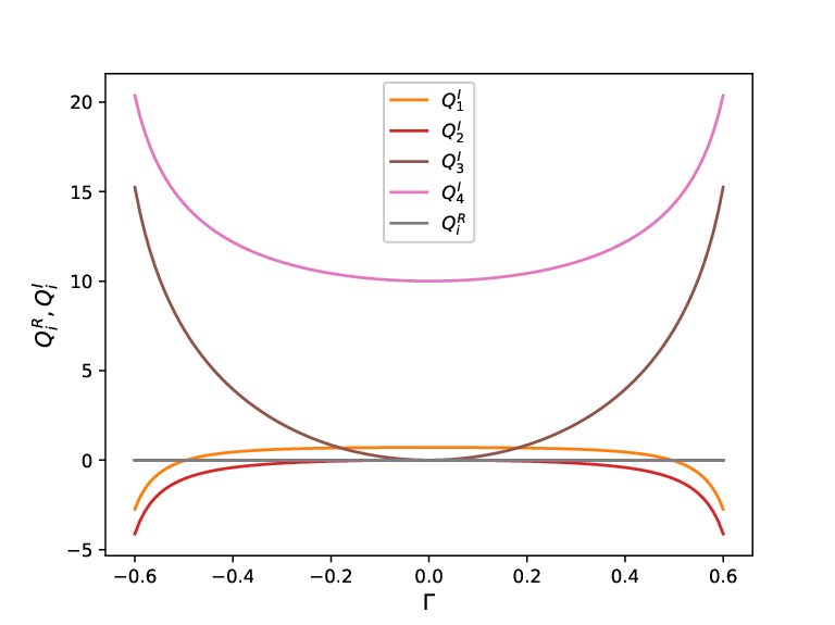
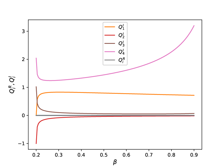
It is observed numerically that the $Q_{i}^{R}\sim{\cal{O}}(10^{-16})\ \forall\ i$ with an upper bound on the computational error of the same order, while the $Q_{i}^{I}$ take non-zero finite values for the fixed $\beta$ and $-\frac{1}{\sqrt{2}}<\Gamma<\frac{1}{\sqrt{2}}$ , where the $Q_{j}$ is written in terms of real and imaginary parts as $Q_{j}=Q_{j}^{R}+iQ_{j}^{I}$ . Plots of the $Q_{i}$ ’s as a function of the $\Gamma$ for fixed $\beta=.99$ is given in the Fig. (1(a)) and the $Q_{i}$ ’s versus $\beta$ for $\Gamma=.1$ is given in the Fig. (1(b)). It has been checked numerically for other values of $\Gamma$ and $\beta$ satisfying (21) that the same results hold. Eq. (34) can be solved analytically by assuming $Q_{i}^{R}=0\ \forall\ i$ for which ${|A_{0}|}$ and ${|B_{0}|}$ are constants of motion. In particular, taking the constant values of $A_{0}$ and $B_{0}$ as their values at $t=0$ , i.e. $A_{0}\equiv A_{0}(0),B_{0}\equiv B_{0}(0)$ , the solutions are obtained as,

	$\displaystyle A_{0}(t)={\|A_{0}(0)\|}e^{-3i\alpha t\left[Q_{1}^{I}{\|A_{0}(0)\|}^{2}+2Q_{2}^{I}{\|B_{0}(0)}^{2}\right]},$
	$\displaystyle B_{0}(t)={\|B_{0}(0)\|}e^{-3i\alpha t\left[2Q_{3}^{I}{\|A_{0}(0)\|}^{2}+Q_{4}^{I}{\|B_{0}(0)}^{2}\right]}.$		(36)

The expressions for $Q_{i}^{I}$ are not reproduced, since they are too long and does not add much qualitative information to the discussions. The values of the constants ${|A_{0}(0)|}$ and ${|B_{0}(0)|}$ may be fixed by using initial conditions. The approximate solution is,

	$\displaystyle X$	$\displaystyle=$	$\displaystyle{\|A_{0}(0)\|}\ e^{-it\left[{\lambda_{1}}+3\alpha\left(Q_{1}^{I}{\|A_{0}(0)\|}^{2}+2Q_{2}^{I}{\|B_{0}(0)\|}^{2}\right)\right]}\begin{pmatrix}1\\ \eta_{1}\end{pmatrix}$		(37)
		$\displaystyle+$	$\displaystyle{\|B_{0}(0)\|}\ e^{-it\left[{\lambda_{2}}+3\alpha\left(2Q_{3}^{I}{\|A_{0}(0)\|}^{2}+Q_{4}^{I}{\|B_{0}(0)\mid}^{2}\right)\right]}\begin{pmatrix}1\\ \eta_{2}\end{pmatrix}+c.c.+{\cal{O}}(\alpha).$		(37)

The solution is bounded and consistent with linear stability analysis. The presence of multiple time scales in the solution is apparent, since phases and the amplitudes vary with different time scales. The solutions are uniform for $t\leq\alpha^{-2}$ . The particular solutions of Eq. (32) can be obtained by substituting $A_{0}(t)$ and $B_{0}(t)$ in $B$ . However, a complete solution which is uniform for $t\leq\alpha^{-3}$ requires to find the time dependence of $A_{1}(T_{1})$ and $B_{1}(T_{1})$ appearing in the complementary solution of $X^{(1)}$ . This involves removing secular terms of differential equations appearing at ${\cal{O}}(\alpha^{2})$ , which is beyond the scope of this article.

A comment is in order regarding the choice of the perturbation terms. There are other possibilities for choosing small parameters to implement a perturbation scheme. A few viable perturbation schemes are, (a) $\beta<<1,\alpha<<1$ , (b) $\Gamma<<1,\alpha<<1$ and (c) $\Gamma<<1,\beta<<1$ .

•

Case (a): A multiple scale analysis does not give any bounded solution. The zeroth order system consists of damped and anti-damped oscillators without any coupling between the two. There are growing as well as decaying modes. This is consistent with the results of linear stability analysis which predicts periodic solutions only for $\Gamma^{2}<\beta^{2}$ . However, this condition is violated if $\beta$ is treated as small parameter, while keeping $\Gamma$ arbitrary.
•

Case (b): A multiple scale analysis gives bounded solution that is consistent with linear stability analysis. The perturbative analysis is valid for weak nonlinear interaction characterized by $\alpha<<1$ and is described in Appendix-I.
•

Case (c): The perturbation analysis is valid for strong as well as weak nonlinearity characterized by $\alpha$ . It may be noted that the discussion of this section as well the case (b) is restricted to weak $\alpha$ only. It also deserves special attention due to its relevance in the context of effective dimer model with balanced loss and gain which is treated separately in Sec. 5.

All three cases correspond to perturbation around the point $P_{0}$ . A perturbation around the points $P_{1}^{\pm}$ is not pursued in this article, since it involves use of the Jacobi elliptic functions and the analysis of the equation governing the dynamics of the amplitude becomes nontrivial. However, numerical solutions around the points $P_{1}^{\pm}$ are provided in the next section.

4 Numerical Solution

The linear stability analysis of Eq. (9) predicts periodic solution in regions of the parameter space defined by Eqs. (21) and (24). The perturbative solution obtained by using multiple time scale analysis is also periodic in the lowest order of the perturbation. In absence of any global stability analysis, stability is not guaranteed for the complete Hamiltonian including nonlinear interaction. Further, the system may admit chaotic solution, since the first equation of Eq. (9) may be interpreted as a forced Duffing oscillator with the identification of $\beta y$ as a forcing term whose profile is determined in a nontrivial way by the system itself. Thus, the system may admit chaotic solution for certain regions in the parameter space. In this section, regular as well as chaotic dynamics of Eq. (9) are studied numerically.

The system is described in terms of three independent parameters $\Gamma,\beta$ and $\alpha$ . Bifurcation diagram may be investigated by varying one of these parameters and keeping the remaining two parameters as fixed. The bifurcation diagram for varying $\beta$ is presented in Fig-2 for $\Gamma=0.01$ and $\alpha=.5$ with the initial values of the dynamical variables near the point $P_{0}$ .

The plot is presented for $\beta\geq 0$ . However, it should be mentioned that the bifurcation diagram is symmetric with respect to $\beta=0$ , if extended to negative values of $\beta$ . The onset of chaos is seen for a critical value $\beta_{c}\sim 1.05$ and persists for $\beta\geq\beta_{c}$ . The crossover from regular to chaotic dynamics as $\beta$ is varied through $\beta_{c}$ may be understood by interpreting the $x$ degree of freedom as describing a forced duffing oscillator with the identification of $\beta y$ as the forcing term. Unlike the standard forced Duffing oscillator, the forcing is determined in a nontrivial way from the solution of the system. The chaotic behaviour of $y$ degree of freedom is induced via its coupling to the $x$ degree of freedom. Regular and the chaotic dynamics of the system are studied in some detail in the next two sections. It should be mentioned here that the numerical investigations have been carried out for very large values of $t(\sim 2,000-20,000)$ starting from $t=0$ . However, for better presentations of the plots, figures are shown for an upper range of $t(\sim 100-2000)$ such that the qualitative features are not lost.

4.1 Regular Dynamics

The time-series of the dynamical variables in the vicinity of the point $P_{0}$ is shown in Fig. (3) for $\Gamma=.2,\beta=.5$ and $\alpha=\pm 1$ . Periodic solutions in Figs.(3(a)) and (3(b)) correspond to $\alpha=1$ , while Figs. (3(c)) and (3(d)) correspond to $\alpha=-1$ .

It may be noted that the time evolution of the dynamical variables with the same initial conditions and fixed $\Gamma,\beta$ show similar oscillatory behaviour for positive as well as negative $\alpha$ . There are minute changes in amplitudes and phases and that too in the limit of large $t$ . It has been checked numerically that the same feature also persists for smaller as well as higher values of $\alpha$ . The periodic solutions in the vicinity of the points $P_{1}^{\pm}$ exist only for $\alpha>0$ , confirming the results of the linear stability analysis. The solutions around $P_{1}^{+}$ are shown in Fig. (4) for $\alpha=1,\beta=1.01,\Gamma=.3$ . The Lyapunov exponents and the autocorrelation functions for the time series representing the periodic solutions in Fig. (4) have been calculated to confirm that these solutions are indeed regular. The transition from regular to chaotic behaviour is seen as $\beta$ is increased beyond $\tilde{\beta}_{c}\sim 1.1$ under similar conditions, i.e. $\alpha=1,\gamma=.3$ and $x(0)=.2,y(0)=-0.1,\dot{x}(0)=.02$ and $\dot{y}(0)=.03$ . It may be noted that the initial conditions for the bifurcation diagram in Fig.-2 is different from the initial conditions used for periodic solutions around the point $P_{1}$ in Fig.-4. Thus, the critical value of $\beta_{c}$ is different for the two cases. The equilibrium points

$P_{1}^{\pm}$ are related to each other as $P_{1}^{-}=-P_{1}^{+}$ for fixed $\alpha$ and $\beta$ . Further, Eq. (9) remains invariant under $x\rightarrow-x,y\rightarrow-y$ . Thus, the solutions around the equilibrium point $P_{1}^{-}$ for the same values of the parameters $\alpha=1,\beta=1.01,\gamma=.3$ , but with the initial conditions $x(0)=-.2,y(0)=0.1,\dot{x}(0)=-.02$ and $\dot{y}(0)=-.03$ may simply be obtained by taking mirror image of the plot in Fig. 4.(a) with respect to $x=0$ and in Fig. 4.(b) with respect to $y=0$ . No separate numerical solution around $P_{1}^{-}$ is presented for this reason.

4.2 Chaotic Dynamics

The bifurcation diagram shows that the system with $\Gamma=0.01$ and $\alpha=.5$ is chaotic for $\beta>\beta_{c}=1.05$ . The sensitivity of the dynamical variables to the initial conditions are studied in different regions of the parameters by considering two sets of initial conditions: (a) $x(0)=.01,y(0)=0.02,\dot{x}(0)=.03,\dot{y}(0)=.04$ and (b) $x(0)=.01,y(0)=0.02,\dot{x}(0)=.03,\dot{y}(0)=.025$ . These two initial conditions are identical except for the values of $\dot{y}(0)$ which differ by $.015$ . The time series of the dynamical variables in the chaotic regime is presented in Fig. 5 for $\beta=1.5$ . The chaotic behaviour in the model has been confirmed by other independent methods also. In this regard, the auto-correlation function, Lyapunov exponent, Poincar $\acute{e}$ section and power spectra are plotted in Fig. (6).

The Lyapunov exponents are $(.13248,.0015691,-.0016145,-.13244)$ . The sum of the Lyapunov exponents are zero for a Hamiltonian system which is valid for the present case if values up to the third decimal places are considered with an error of the order of $10^{-4}$ .

The main emphasis of this article is on Hamiltonian system with balanced loss and gain. However, the Hamiltonian with $\Gamma=0$ , i.e. no gain-loss regime, deserves special attention due to its rich dynamical properties. For $\Gamma=0$ , the point $P_{0}$ is stable for $0<\beta^{2}<1$ , while the points $P_{1}^{\pm}$ are stable for $\beta^{2}>1$ . Further, the quantities $Q_{i}$ ’s are purely imaginary and Eq. (34) is exactly solvable without any assumptions on $Q_{i}$ ’s. It has been checked numerically that periodic solutions of Eq. (9) exist for $\Gamma=0$ near the equilibrium points $P_{0}$ , $P_{1}^{\pm}$ . The most important result is that the Hamiltonian $\tilde{H}$ with $\Gamma=0$ is chaotic. The Poincar $\acute{e}$ section, Lyapunov exponents, autocorrelation functions and power spectra for $\Gamma=0,\alpha=.5,\beta=1.5$ and the initial conditions $x(0)=.01,y(0)=.02,\dot{x}(0)=.03,\dot{y}(0)=.04$ are presented in Fig.-7. The Lyapunov exponents are $(0.22685,0.0043114,-.0043114,-0.22685)$ which may be used to compute other measures of a physical system. The highest Lyapunov exponent for $\Gamma=0$ is greater than the highest Lyapunov exponent for $\Gamma=.01$ with all other conditions remaining the same.

It may be noted that the Duffing oscillator admits chaotic solutions provided both damping and external driving terms are present. However, for the case of coupled Duffing oscillator model of this article, chaotic behaviour is observed for the system without any loss-gain terms. The coupling to the linear oscillator with $x$ -dependent angular frequency provides driving force to the Duffing oscillator. The Hamiltonian $H_{u}$ in Eq. (6) takes a simple form for $\gamma=0,\beta_{1}=\beta_{2}$ :

\displaystyle H_{u}=\left(\frac{1}{2}P_{u}^{2}+\frac{\Omega_{+}}{2}u^{2}+\frac{g}{4}u^{4}\right)-\left(\frac{1}{2}P_{v}^{2}+\frac{\Omega_{-}}{2}v^{2}+\frac{g}{4}v^{4}\right)+\frac{g\ uv}{2}\left(u^{2}-v^{2}\right),\Omega_{\pm}=\omega^{2}\pm\beta_{1}.

(38)

describing two nonlinearly coupled undamped unforced Duffing oscillators. This also provides an example of Hamiltonian chaos within a simple framework which deserves further investigations.

5 Non- ${\cal{PT}}$ -symmetric Dimer with balanced loss and gain

Different types of dimer models play an important role in many areas of physics and in particular, in the context of ${\cal{PT}}$ symmetric systems[4, 6, 12, 22, 23]. In this section, an exactly solvable non- ${\cal{PT}}$ -symmetric Hamiltonian describing a dimer model with balanced loss and gain is shown to admit periodic solutions. A standard route to the occurrence of dimer models is via different approximation methods, including the multiple time scale analysis. The time-evolution of the amplitude in the leading order of the perturbation is described by dimer models. For the case of the coupled Duffing oscillator model, the resulting dimer models for $\alpha\ll 1$ in Eq. (34) and for $\gamma\ll 1,\alpha\ll 1$ in Eq. (61) do not contain any loss-gain terms. A dimer model with balanced loss and gain is obtained for $\Gamma\ll 1,\beta\ll 1$ that is described in this section.

Both $\Gamma$ and $\beta$ are treated as small parameters with the identification of $\Gamma\equiv\epsilon^{2}\Gamma_{0},\beta\equiv\epsilon^{2}\beta_{0},\ \epsilon\ll 1$ . The strength of the nonlinear interaction $\alpha$ is kept arbitrary. The time scales and power series expansion of the space co-ordinates in terms of $\epsilon$ are chosen as,

\displaystyle T_{0}=t,T_{2n}=\epsilon^{2n}t,n=1,2,\dots,\ \ X=\sum_{n=0}^{\infty}\epsilon^{2n+1}X^{(2n+1)},

(39)

so that there is no contribution from the nonlinear interaction in the lowest order. In particular, after using Eq. (39), the lowest two orders of the equations of motion (27) read,

	$\displaystyle{\cal{O}}(\epsilon):\ \ \frac{\partial^{2}X^{(1)}}{\partial T_{0}^{2}}+X^{(1)}=0,$		(40)
	$\displaystyle{\cal{O}}(\epsilon^{3}):\ \ \frac{\partial^{2}X^{(3)}}{\partial T_{0}^{2}}+X^{(3)}+2\frac{\partial^{2}X^{(1)}}{\partial T_{0}\partial_{2}}+2\Gamma_{0}\sigma_{3}\frac{\partial{X}^{(1)}}{\partial T_{0}}+\beta_{0}\sigma_{1}X^{(1)}+\alpha\begin{pmatrix}{x_{1}}^{3}\\ 3{x_{1}}^{2}y_{1}\end{pmatrix}=0.$		(41)

The ${\cal{O}}(\epsilon)$ equation describes two decoupled isotropic harmonic oscillators and the general solution has the form

\displaystyle X^{(1)}=A(T_{2},T_{4},\dots)e^{iT_{0}}+c.c.,\ \ A\equiv\begin{pmatrix}A_{1}(T_{2},\dots)\\ B_{1}(T_{2},\dots)\end{pmatrix},

(42)

where the amplitude $A$ depends on slower time scales. The time-evolution of $A$ as a function of $T_{2}$ is determined by the equation²² 2 A detailed derivation is skipped in order to avoid repetition. The necessary steps as outlined in Sec. 3 for the case of $\alpha\ll 1$ may be followed to derive this equation.,

\displaystyle 2i\frac{\partial A}{\partial T_{2}}+\left(2i\Gamma_{0}\sigma_{3}+\beta_{0}\sigma_{1}\right)A+3\alpha\begin{pmatrix}{|A_{1}|}^{2}A_{1}\\ 2{|A_{1}|}^{2}B_{1}+A_{1}^{2}B_{1}^{*}\end{pmatrix}=0,

(43)

which is obtained by substituting $X^{(1)}$ in Eq. (41) and removing the secular terms. Eq. (43) describes a coupled dimer model with nonlinear interaction. The amplitudes $A_{i}$ ’s may be identified as wave propagating along the $i^{th}$ wave-guide.

Eq. (43) may also be derived from the Lagrangian ${\cal{L}}$ or the corresponding Hamiltonian ${\cal{H}}$ ,

	$\displaystyle{\cal{L}}=\frac{i}{2}\left(A^{\dagger}\sigma_{1}\dot{A}-\dot{A}^{\dagger}\sigma_{1}A\right)-2\Gamma_{0}A^{\dagger}\sigma_{2}A-\beta_{0}A^{\dagger}A-3\alpha{\|A_{1}\|}^{2}\left(A_{1}B_{1}^{}+A_{1}^{}B_{1}\right),$
	$\displaystyle{\cal{H}}=2\Gamma_{0}A^{\dagger}\sigma_{2}A+\beta_{0}A^{\dagger}A+3\alpha{\|A_{1}\|}^{2}\left(A_{1}B_{1}^{}+A_{1}^{}B_{1}\right).$		(44)

The canonically conjugate variables are $(A_{1},iB_{1}^{*})$ . The Hamiltonian system describes a nonlinear Schr $\ddot{o}$ dinger dimer with balanced loss and gain. The parameter $\Gamma_{0}$ measures the strength of the loss-gain, while $\alpha$ is the coupling of the nonlinear interaction. The system differs with most of the previous studies on Hamiltonian dimer model with balanced loss and gain in one respect, it is not ${\cal{PT}}$ symmetric. The parity and time-reversal transformation are defined as, ${\cal{P}}:A\rightarrow\sigma_{1}A,\ {\cal{T}}:T_{2}\rightarrow-T_{2},i\rightarrow-i$ . The Hamiltonian is ${\cal{PT}}$ symmetric for $\alpha=0$ . The nonlinear interaction breaks ${\cal{PT}}$ symmetry and ${\cal{H}}$ is non- ${\cal{PT}}$ -symmetric for $\alpha\neq 0$ .

The Hamiltonian dimer is an integrable system. Introducing the Stokes variables,

\displaystyle Z_{a}=2A^{\dagger}\sigma_{a}A,\ R=2A^{\dagger}A=\sqrt{Z_{1}^{2}+Z_{2}^{2}+z_{3}^{2}},\ a=1,2,3,

(45)

it immediately follows from Eq. (43) that $Z_{1}$ is the second integral of motion, i.e. $\dot{Z_{1}}=0$ . The constant $Z_{1}$ is fixed to its initial value at $T_{2}=0$ , i.e. $Z_{1}(0)\equiv C_{1}$ . The dimer equations are transformed into a set of coupled linear differential equation,

\displaystyle\dot{Z}=NZ,\ \ Z\equiv\begin{pmatrix}Z_{2}\\ Z_{3}\\ R\end{pmatrix},\ \ N\equiv\begin{pmatrix}0&&a&&b\\ -a&&0&&-c\\ b&&-c&&0\end{pmatrix},

(46)

where the parameters $a,b,c$ are defined as,

\displaystyle a=\beta_{0}+\frac{3\alpha C_{1}}{4},\ b=\frac{3\alpha C_{1}}{4},\ c=2\Gamma_{0}.

(47)

One of the eigenvalues of the matrix $N$ is zero and the remaining two eigenvalues are purely imaginary numbers and complex conjugate of each other for real $\eta$ :

\displaystyle\eta_{1}=0,\eta_{2}=i\eta,\eta_{3}=-i\eta,\ \ \eta\equiv\sqrt{a^{2}-b^{2}-c^{2}}=\sqrt{\left(\beta_{0}^{2}+\frac{3}{2}\alpha\beta_{0}C_{1}\right)-4\Gamma_{0}^{2}}.

(48)

There are growing as well as decaying modes whenever $\eta$ becomes imaginary. The parameter $\eta$ is real for the following condition,

\displaystyle\beta_{0}^{2}+\frac{3}{2}\alpha\beta_{0}C_{1}-4\Gamma_{0}^{2}\geq 0.

(49)

It is interesting to note that for a fixed set of parameters the integration constant $C_{1}$ may be always chosen such that $\eta$ is real. The general solutions has the expression,

\displaystyle Z=C_{2}\begin{pmatrix}-\frac{c}{a}\\ -\frac{b}{a}\\ 1\end{pmatrix}+C_{3}\begin{pmatrix}i\frac{-a(ab-ic\eta)+b(b^{2}+c^{2})}{(b^{2}+c^{2})\eta}\\ -\frac{ab-ic\eta}{b^{2}+c^{2}}\\ 1\end{pmatrix}e^{-i\eta\epsilon^{2}t}+C_{4}\begin{pmatrix}i\frac{a(ab+ic\eta)-b(b^{2}+c^{2})}{(b^{2}+c^{2})\eta}\\ -\frac{ab+ic\eta}{b^{2}+c^{2}}\\ 1\end{pmatrix}e^{i\eta\epsilon^{2}t},

(50)

where $C_{2},C_{3},C_{4}$ are integration constants. The solutions for $A_{1}$ and $A_{2}$ may be obtained as,

\displaystyle A_{1}=\frac{1}{2}\sqrt{R+Z_{3}}\ e^{i\theta_{1}},\ A_{2}=\frac{1}{2}\sqrt{R-Z_{3}}\ e^{i\theta_{2}},

(51)

where the phases are determined from the equations,

\displaystyle\frac{d\theta_{1}}{dT_{2}}=\frac{\beta_{0}}{2}\frac{Z_{1}}{R+Z_{3}}+\frac{3}{4}(R+Z_{3}),\ \ \theta_{2}=\theta_{1}+\tan^{-1}\frac{Z_{2}}{Z_{1}}.

(52)

The expressions for the amplitudes ${|A_{i}|}$ and the relative phase $\theta_{1}-\theta_{2}$ are derived from the defining relations for the Stokes variables. On the other hand, time-evolution of $\theta_{1}$ is determined from Eq. (43) by using $A_{j}={|A_{j}|}e^{i\theta_{j}},j=1,2$ . The four integration constants $C_{i}$ may be chosen appropriately to implement a variety of initial conditions. There may be restrictions on the parameters for specified initial conditions such that ${|A_{1}|},{|A_{2}|}$ are semi-positive definite and phases are well defined.

The system admits a stationary mode for which $A_{1},A_{2}$ are periodic in time with constant amplitudes. In particular, the amplitudes ${|A_{1}|},{|A_{2}|}$ are independent of time, while the phases depend on time. The stationary solution is obtained by choosing the integration constants as $C_{2}=\frac{a}{\eta}C_{1},C_{3}=C_{4}=0$ for which $Z^{T}=\frac{C_{1}}{\eta}(-c,-b,a)$ and the integration constant $C_{1}$ may be fixed through appropriate initial condition. The expressions for $A_{1},A_{2}$ corresponding to this particular solution of $Z$ are obtained by using Eqs. (51) and (52),

	$\displaystyle A_{1}$	$\displaystyle=$	$\displaystyle\sqrt{\frac{C_{1}\beta_{0}}{\eta}}\ e^{i\frac{2\eta^{2}+3C_{1}\beta_{0}}{4\eta}\epsilon^{2}t},$
	$\displaystyle A_{2}$	$\displaystyle=$	$\displaystyle\sqrt{\frac{C_{1}}{2\eta}(2\beta_{0}+3\alpha C_{1})}\ \ e^{i\left[\frac{2\eta^{2}+3C_{1}\beta_{0}}{4\eta}-\tan^{-1}\left(\frac{2\Gamma_{0}}{\eta}\right)\right]\epsilon^{2}t}.$		(53)

These solutions are physically acceptable in regions of the parameter-space determined by Eq.(49) along with the additional conditions:

\displaystyle\textrm{For}\ \ \alpha\geq 0:C_{1}\beta_{0}>0,\ \ \textrm{For}\ \ \alpha<0:0<C_{1}\beta_{0}<\frac{2\beta_{0}^{2}}{3{|\alpha|}}.

(54)

It may be noted that $C_{1}$ can always be chosen satisfying these conditions for any given set of values for $\alpha,\beta_{0},\Gamma_{0}$ . The power $P_{i}={|A_{i}|}^{2}$ for the $i^{th}$ wave-guide remains the same throughout the time-evolution, without being effected by the loss gain terms. Such a stationary mode, which exists for ${\cal{PT}}$ -symmetric dimer models, is also seen in this non- ${\cal{PT}}$ -symmetric Hamiltonian system. Moreover, the allowed ranges of $\Gamma_{0}$ can be varied at ease by choosing appropriate value of the integration constant $C_{1}$ for a fixed set of parameters $\alpha$ and $\beta$ . This is an advantage over the previous models.

Solutions with time-dependent amplitude as well as phase can also be constructed. For example, the initial profile $Z(0)^{T}=(0,0,1)$ may be implemented by choosing $C_{1}=\frac{2}{3\alpha\Gamma_{0}}(1-2\Gamma_{0}\beta_{0}),C_{2}=\frac{a^{2}}{\eta^{2}},C_{3}=C_{4}=-\frac{b^{2}+c^{2}}{2\eta^{2}}$ for which $Z(t)$ has the following expression:

\displaystyle Z(t)=\frac{1}{\eta^{2}}\begin{pmatrix}1\\ ab\\ \eta^{2}-a^{2}\end{pmatrix}\cos(\eta\epsilon^{2}t)-\frac{1}{\eta^{2}}\begin{pmatrix}1\\ ab\\ -a^{2}\end{pmatrix}+\frac{1}{\eta}\begin{pmatrix}b\\ -c\\ 0\end{pmatrix}\sin(\eta\epsilon^{2}t).

(55)

The solution for $A_{1},A_{2}$ may be determined by using the Eqs. (51) and (52). The Hamiltonian ${\cal{H}}$ is not ${\cal{PT}}$ symmetric, yet it admits periodic solutions. This ascertains that systems with balanced loss and gain may admit periodic solutions without any ${\cal{PT}}$ symmetry of the governing Hamiltonian. The periodic solutions become unbounded for the values of the parameter for which $\eta$ is imaginary. The corresponding solutions in terms of hyperbolic functions may be obtained by taking the limit $\eta\rightarrow i\eta$ in $Z(t)$ .

6 Conclusions $\&$ Discussions

It has been shown that a non- ${\cal{PT}}$ symmetric Hamiltonian system with balanced loss and gain may admit stable periodic solutions in some regions of the parameter-space. The result is important from the viewpoint that all previous investigations are mainly based on ${\cal{PT}}$ -symmetric systems in which the existence of stable periodic solution is attributed to the unbroken ${\cal{PT}}$ -phase. The requirement of ${\cal{PT}}$ symmetry is too restrictive and there is no compelling reason for a system with balanced loss and gain to be ${\cal{PT}}$ -symmetric in order to admit stable periodic solutions. The result of this article paves the way for accommodating a large class of non- ${\cal{PT}}$ symmetric Hamiltonian in the mainstream of investigations on systems with balanced loss and gain. Further, all the advantages associated with a Hamiltonian system may be used to explore such a model in detail.

A coupled Duffing oscillator Hamiltonian system with balanced loss and gain has been considered as an example to present the results. The Duffing oscillator is coupled to an anti-damped harmonic oscillator such that the coupling term effectively acts as a forcing term, albeit in a non-trivial way. The frequency of the anti-damped oscillator depends on the degree of freedom corresponding to the Duffing oscillator. There is an interesting limit in which the dynamics of the Duffing oscillator completely decouples from the system, while the anti-damped oscillator is unidirectionally coupled to it. This limit corresponds to a Hamiltonian formulation for the standard Duffing oscillator. It should be emphasized that even in this limit the anti-damped oscillator is not a time-reversed version of the standard Duffing oscillator. This opens the possibility of investigating the dynamics of the standard Duffing oscillator using techniques associated with a Hamiltonian system. Further, the quantum Duffing oscillator may also be introduced and investigated within the canonical quantization scheme.

It has been shown that the coupled Duffing oscillator model admits stable periodic solution in some regions of the parameter-space. The Hamiltonian is non- ${\cal{PT}}$ -symmetric and there is no question of attributing these periodic solutions to an unbroken ${\cal{PT}}$ -phase. These solutions are investigated by using perturbative as well as numerical methods. It is known that the driven Duffing oscillator admits chaotic behaviour. The coupled Duffing oscillator model investigated in this article also admits chaotic behaviour in some regions of the parameter-space where the coupling to the anti-damped oscillator effectively acts as a driving term. This is an example of a Hamiltonian chaos for systems with balanced loss and gain which has not been observed earlier.

The method of multiple scale analysis has been used to investigate the system perturbatively. The amplitude depends on a slower time-scale than the phase and the dynamics of the amplitude is determined by a set of coupled nonlinear equations which describe a dimer system. The resulting dimer model in the leading order of the perturbation for small coupling $\beta$ and loss-gain parameter $\Gamma$ is also Hamiltonian and non- ${\cal{PT}}$ symmetric. Further, it is exactly solvable and admits stable periodic solutions in some regions of the parameters space. This provides an example of a non- ${\cal{PT}}$ -symmetric dimer model admitting stable periodic solution. It should be mentioned here that the dimer model obtained by considering the nonlinear coupling $\alpha$ as a small parameter is also non- ${\cal{PT}}$ symmetric and no exact solutions can be found for the generic values of $\beta$ and $\Gamma$ . However, stable periodic solutions are obtained for $\Gamma$ and $\beta$ within a range specified by the linear stability analysis. It is known that dimer models with balanced loss and gain are important in the field of optics and provide many counter-intuitive results. The examples provided in this article suggest that non- ${\cal{PT}}$ -symmetric systems should be included within the ambit of the investigations on dimer models with balanced loss and gain

It is worth recalling some of the results pertaining to ${\cal{PT}}$ -symmetric quantum systems [13, 14, 15, 16, 20, 21] to place the results obtained in this article in proper perspective. The general understanding on non-hermitian quantum system is that it may admit entirely real spectra with unitary time-evolution provided at least one of the following conditions is satisfied:

•

The Hamiltonian is ${\cal{PT}}$ symmetric and unbroken ${\cal{PT}}$ -phase exists[13]. It may be noted in this context that, unlike in the case of classical mechanics, the time-reversal symmetry is not unique for quantum system. The non-conventional representation of the time-reversal operator ${\cal{T}}$ has been used in the literature[7, 8].
•

The Hamiltonian $H$ is pseudo-hermitian with respect to a positive-definite similarity operator $\eta$ , i.e. $H^{\dagger}=\eta H\eta^{-1}$ [14], where $H^{\dagger}$ denotes the hermitian adjoint of $H$ . The system admits an anti-linear symmetry[14] which may be identified as ${\cal{PT}}$ symmetry for some special cases. This allows to include non- ${\cal{PT}}$ -symmetric Hamiltonians with pseudo-hermiticity or with specific anti-linear symmetry in the main stream of investigations on non-hermitian systems admitting entirely real spectra and unitary time-evolution[20, 21].

The situation changes significantly for a classical system for which the time-reversal symmetry is unique and there is no analogue of pesudo-hermiticity or anti-linear symmetry for the classical Hamiltonian. It appears that the criterion based on ${\cal{PT}}$ -symmetry alone is not sufficient to predict the existence of periodic solution in a classical balanced loss-gain system. A possible resolution of the problem may be to fix the criterion based on the corresponding quantum system so that anti-linear symmetry and/or pseudo-hermiticity of the quantized Hamiltonian is used. However, an implementation of the scheme is tricky and nontrivial, since there may be more than one quantum system for a given classical Hamiltonian based on the quantization condition. A unique identification of the quantized Hamiltonian corresponding to a given classical system with balanced loss and gain that admits periodic solution requires additional conditions to be imposed. The problem to fix an appropriate criterion for the existence of periodic solution in classical system with balanced loss and gain remains unresolved and requires further investigations.

7 Acknowledgements

This work of PKG is supported by a grant (SERB Ref. No. MTR/2018/001036) from the Science & Engineering Research Board(SERB), Department of Science & Technology, Govt. of India under the MATRICS scheme. The work of PR is supported by CSIR-NET fellowship(CSIR File No.: 09/202(0072)/2017-EMR-I) of Govt. of India.

8 Appendix-I: Perturbative solution for $\Gamma\ll 1,\alpha\ll 1$

Introducing a small parameter $\epsilon\ll 1$ and defining $\Gamma=\epsilon\Gamma_{0},\alpha=\epsilon\alpha_{0}$ , Eq. (27) can be rewritten as,

\displaystyle\ddot{X}+PX+\epsilon\left[2\Gamma_{0}\sigma_{3}\dot{X}+\alpha_{0}\tilde{V}(x)\right]=0.

(56)

The unperturbed part of the system is described by coupled harmonic oscillators satisfying the equation $\ddot{X}+PX=0$ . The terms with the coefficient $\epsilon$ in Eq. (56) is treated as perturbation, which contain the effect of loss-gain and nonlinear coupling. The standard perturbation theory fails and the method of multiple time-scales will be employed to analyse Eq. (56). The coordinates are expressed in powers of the small parameter $\epsilon$ and multiple time-scales are introduced as follow,

\displaystyle T_{n}=\epsilon^{n}t,\ \ X=\sum_{n=0}^{\infty}\epsilon^{n}X^{(n)}(T_{0},T_{1},\dots).

(57)

Using Eq. (57) in Eq. (56) and equating the terms with same coefficient $\epsilon^{n}$ to zero, the following equations up to $O(\epsilon)$ are obtained as follows:

	$\displaystyle{\cal{O}}(\epsilon^{0}):$		$\displaystyle\frac{\partial^{2}X^{(0)}}{\partial T_{0}^{2}}+PX^{(0)}=0,$		(58)
	$\displaystyle{\cal{O}}(\epsilon):$		$\displaystyle\frac{\partial^{2}X^{(1)}}{\partial T_{0}^{2}}+PX^{(1)}+2\frac{\partial^{2}X^{(0)}}{\partial T_{0}\partial T_{1}}+2\Gamma_{0}\sigma_{3}\frac{\partial X^{(0)}}{\partial T_{0}}+\alpha_{0}\begin{pmatrix}x_{0}^{3}\\ 3x_{0}^{2}y_{0}\end{pmatrix}=0.$		(59)

These equations are to be solved consistently to get the perturbative results.

The unperturbed Eq. (58) has the solution,

\displaystyle X^{(0)}=A_{0}\ e^{-i{\chi_{1}}T_{0}}\begin{pmatrix}1\\ \beta\end{pmatrix}+B_{0}\ e^{-i{\chi_{2}}T_{0}}\begin{pmatrix}1\\ -\beta\end{pmatrix}+c.c.,\ \chi_{1}=\sqrt{1+\beta},\ \chi_{2}=\sqrt{1-\beta}.

(60)

The $T_{1}$ dependence of $A_{0}$ and $B_{0}$ are determined by the equations,

\displaystyle\frac{\partial A_{0}}{\partial T_{1}}=-\frac{3i\alpha_{0}}{\chi_{1}}{|A_{0}|}^{2}A_{0},\ \ \frac{\partial B_{0}}{\partial T_{1}}=-\frac{3i\alpha_{0}}{\chi_{2}}{|B_{0}|}^{2}B_{0},\ \

(61)

which have been obtained by eliminating secular terms of Eq. (59). These two equations define a Hamiltonian system,

\displaystyle{\cal{H}}_{1}=3\alpha_{0}\left[\frac{{|A_{0}|}^{4}}{\chi_{1}}+\frac{{|B_{0}|}^{4}}{\chi_{2}}\right],

(62)

with the canonical conjugate pairs as $(A_{0},iA_{0}^{*})$ and $(B_{0},iB_{0}^{*})$ . It immediately follows that both ${|A_{0}|}$ and ${|B_{0}|}$ are constants of motion and the constant values are chosen to be their value at $t=0$ . The approximate solution of $X$ is obtained as,

\displaystyle X={|A_{0}(0)|}\ e^{-it\left[{\chi_{1}}+\frac{3\alpha{|A_{0}(0)|}^{2}}{\chi_{1}}\right]}\begin{pmatrix}1\\ \beta\end{pmatrix}+{|B_{0}(0)|}\ e^{-it\left[{\chi_{2}}+\frac{3\alpha{|B_{0}(0)|}^{2}}{\chi_{2}}\right]}\begin{pmatrix}1\\ -\beta\end{pmatrix}+c.c.+{\cal{O}}(\epsilon),

(63)

which is periodic and has uniform expansion for $t\leq\epsilon^{-2}$ . It may be noted that $\alpha=\alpha_{0}\left(\frac{\Gamma}{\Gamma_{0}}\right)$ and the solution inherits the effect of both the loss-gain and nonlinear interaction.

References

[1] C. M. Bender, M. Gianfreda, S. K. Ozdemir, B. Peng, and L. Yang, Twofold transition in PT-symmetric coupled oscillators, Phys. Rev. A 88, 062111 (2013).
[2] B. Peng, S. K. Ozdemir, F. Lei, F. Monifi, M. Gianfreda, G. L. Long, S. Fan, F. Nori, C. M. Bender, and L. Yang, Parity–time-symmetric whispering-gallery microcavities, Nature Physics, 10 394 (2014).
[3] C. M. Bender, M. Gianfreda and S. P. Klevansky, Systems of coupled PT-symmetric oscillators, Phys. Rev A90, 022114 (2014).
[4] I. V. Barashenkov and M. Gianfreda, An exactly solvable $\mathcal{PT}$ -symmetric dimer from a Hamiltonian system of nonlinear oscillators with gain and loss, J. Phys. A: Math. Theor. 47, 282001(2014).
[5] D. Sinha, P. K. Ghosh, ${\cal{PT}}$ -symmetric rational Calogero model with balanced loss and gain, Eur. Phys. J. Plus, 132: 460 (2017), arXiv:1705:03426.
[6] A. Khare, A. Saxena, Integrable oscillator type and Schr $\ddot{o}$ dinger type dimers, J. Phys. A: Math. Theor. 50, 055202 (2017).
[7] P. K. Ghosh and Debdeep Sinha, Hamiltonian formulation of systems with balanced loss-gain and exactly solvable models, Annals of Physics 388, 276 (2018).
[8] D. Sinha, P. K. Ghosh, On the bound states and correlation functions of a class of Calogero-type quantum many-body problems with balanced loss and gain, J. Phys. A: Math. Theor. 52, 505203 (2019).
[9] D. Sinha and P. K. Ghosh, Integrable coupled Li $\acute{e}$ nard-type systems with balanced loss and gain, Annals of Physics 400, 109 (2019).
[10] P. K. Ghosh, Taming Hamiltonian systems with balanced loss and gain via Lorentz interaction : General results and a case study with Landau Hamiltonian, J. Phys. A: Math. Theor. 52, 415202(2019).
[11] Jes $\acute{u}$ s Cuevas, Panayotis G. Kevrekidis, Avadh Saxena and Avinash Khare, PT-symmetric dimer of coupled nonlinear oscillators, Phys. Rev. A 88, 032108 (2013).
[12] D. A. Zezyulin and V. V. Konotop, Nonlinear Modes in Finite-Dimensional ${\cal PT}$ -Symmetric Systems, Phys. Rev. Lett. 108, 213906 (2012).
[13] C. M. Bender and Stefan Boettcher, Real Spectra in Non-Hermitian Hamiltonians Having ${\cal{PT}}$ Symmetry, Phys. Rev. Lett. 80, 5243 (1998).
[14] A. Mostafazadeh, Pseudo-Hermitian representation of quantum mechanics, Int. J. Geom. Methods in Mod. Phys. 7, 1191 (2010).
[15] P. K. Ghosh, On the construction of pseudo-hermitian quantum system with a pre-determined metric in the Hilbert space, J. Phys. A:Math. Theor. 43, 125203, (2010).
[16] M. S. Swanson, Transition elements for a non-Hermitian quadratic Hamiltonian, J. Math. Phys.45, 585 (2004); A. Fring and M. H. Y. Moussa, Non-Hermitian Swanson model with a time-dependent metric, Phys. Rev. A 94, 042128 (2016).
[17] T. Deguchi and P. K. Ghosh, Exactly Solvable Quasi-hermitian Transverse Ising Model, J. Phys. A: Math. Theor. 42, 475208 (2009); T. Deguchi, P. K. Ghosh and Kazue Kudo, Level statistics of a pseudo-Hermitian Dicke model, Phys. Rev. E 80, 026213 (2009); T. Deguchi and P. K. Ghosh, Quantum Phase Transition in a Pseudo- hermitian Dicke model, Phys. Rev. E80, 021107 (2009).
[18] P. K. Ghosh, A note on topological insulator phase in non-hermitian quantum system, J. Phys.: Condens. Matter 24, 145302 (2012); Deconstructing non-dissipative non-Dirac-hermitian relativistic quantum systems, Phys. Lett. A375, 3250 (2011); Deconstructing non-Dirac-hermitian supersymmetric quantum systems, J. Phys. A:Math. Theor. 44, 215307 (2011); Exactly solvable non-hermitian Jaynes-Cummings-type Hamiltonian admitting entirely real spectra from supersymmetry, Journal of Physics A: Mathematical & General 38, 7313 (2005).
[19] P. K. Ghosh, Constructing Exactly Solvable Pseudo-hermitian Many- particle Quantum Systems by Isospectral Deformation, Int. J. Theo. Phys. 50, 1143 (2011).
[20] Rosas-Ortiz, O. Casta $\tilde{n}$ os and D. Schuch, New supersymmetry-generated complex potentials with real spectra, J. Phys. A 48, 445302 (2015); Z. Blanco-Garcia, O. Rosas-Ortiz and K. Zelaya, Interplay between Riccati, Ermakov, and Schr $\ddot{o}$ dinger equations to produce complex-valued potentials with real energy spectrum, Math. Methods Appl. Sci. 42, 4925 (2019).
[21] R. Ramírez and M. Reboiro, Dynamics of finite dimensional non-hermitian systems with indefinite metric, J. Math. Phys. 60, 012106 (2019); R. Ramírez and M. Reboiro, Squeezed states from a quantum deformed oscillator Hamiltonian, Phys. Lett. A 380, 1117 (2016).
[22] Y. Kominis, T. Bountis and S. Flach, The Asymmetric Active Coupler: Stable Nonlinear Supermodes and Directed Transport, Sci. Rep. 6, 33699 (2016).
[23] P. Lunt, D. Haag, D. Dast, H. Cartarius, and G. Wunner, Balanced gain and loss in Bose-Einstein condensates without ${\cal{PT}}$ symmetry, Phys. Rev. A 96, 023614(2017).
[24] C. M. Bender, J. Feinberg, D. W. Hook and D. J. Weir, Chaotic systems in complex phase space. Pramana 73i, 453(2009).
[25] C. T. West, T. Kottos and T. Prosen, ${\cal{PT}}$ symmetric wave chaos, Phys.Rev.Lett. 104, 054102 (2010); S. Mudute-Ndumbe and E.-M. Graefe, Quantum chaos in a non-Hermitian PT-symmetric kicked top, arXiv:1912.09412.
[26] Xin-You L $\ddot{u}$ , Hui Jing, Jin-Yong Ma and Ying Wu, ${\cal{PT}}$ -Symmetry-Breaking Chaos in Optomechanics, Phys. Rev. Lett. 114, 253601 (2015); M. Wang, D. Zhnag, X. Li, Y. Wu, Z. Sun, Magnon Chaos in ${\cal{PT}}$ -symmetric cavity Magnomechanics, IEEE Photonics Journal 11, 5300108 (2019).
[27] S. H. Strogartz, Nonlinear Dynamics and Chaos: With Applications to Physics, Biology, Chemistry and Engineering, CRC Press.
[28] The Duffing Equation: Nonlinear Oscillators and their Behaviour, Edited by I. Kovacic and M. J. Brennan, John Wiley & Sons Ltd., UK.
[29] G. Zhao et. al, Active nonlinear inerter damper for vibration mitigation of Duffing oscillators, Journal of Sound and Vibration 473, 115236 (2020); Q. X. Liu, J.K. Liu, and Y.M. Chen, An analytical criterion for alternate stability switches in nonlinear oscillators with varying time delay, International Journal of Non-Linear Mechanics 126, 103563 (2020); G. M. Moatimid, Stability analysis of a parametric Duffing Oscillator, Journal of Engineering Mechanics 146, 05020001 (2020).
[30] A. H. Nayfeh, Perturbation Methods, Wiley, 1973; P. K. Jakobsen, Introduction to the method of multiple scales, arXiv:1312.3651.
[31] P. G. L. Dirichlet, $\ddot{U}$ ber die Stabilit $\ddot{a}$ t des Gleichgewichts, Crelle 32, 85(1846); R. Krechetnikov and J. E. Marsden, Dissipation-induced instabilities in finite dimensions, Rev. Mod. Phys. 79, 519 (2007).
[32] M. W. Hirsch, S. Smale and R. L. Devany, Differential Equations, Dynamical Systems, and Introduction to chaos, Academic Press (2013); N. R. Lebovitz, Ordinary Differential Equations, Brook/Cole, 1999 (http://people.cs.uchicago.edu/ lebovitz/odes.html).

On regular and chaotic dynamics of a non-𝒫𝒯{\cal{PT}}-symmetric Hamiltonian system of a coupled Duffing oscillator with balanced loss and gain