Jet-based measurements of Sivers and Collins asymmetries
at the future Electron-Ion ColliderPreprint: JLAB-PHY-20-3223
Abstract
We present predictions and projections for hadron-in-jet measurements and electron-jet azimuthal correlations at the future Electron-Ion Collider (EIC). These observables directly probe the three-dimensional (3D) structure of hadrons, in particular, the quark transversity and Sivers parton distributions and the Collins fragmentation functions. We explore the feasibility of these experimental measurements by detector simulations and discuss detector requirements. We conclude that jet observables have the potential to enhance the 3D imaging EIC program.
Keywords:
Electron-Ion Collider, Jets, Three-Dimensional Hadron Structure, Sivers asymmetry, Collins asymmetry, JLAB-PHY-20-3223I Introduction
Jets, collimated sprays of particles, observed in high-energy particle collisions, offer a unique opportunity to study quantum chromodynamics (QCD). Measurements of jets at the Large Hadron Collider (LHC) have triggered the development of new theoretical and experimental techniques for detailed studies of QCD Larkoski:2017jix.
Jet observables can probe the three-dimensional (3D) hadron structure encoded in transverse-momentum-dependent parton-distribution functions (TMD PDFs) and fragmentation functions (TMD FFs). For example, Higgs-plus-jet production at the LHC gives access to the gluon TMD PDF Boer:2014lka, while the hadron transverse-momentum distribution inside jets probes TMD FFs Aad:2011sc; Aaij:2019ctd; Kang:2019ahe. Recently, jet production in deep-inelastic scattering (DIS) regime was proposed as a key channel for TMD studies Gutierrez-Reyes:2018qez; Gutierrez-Reyes:2019vbx; Liu:2018trl; Kang:2020xyq. Jets produced in polarized proton-proton collisions probe the Sivers Boer:2003tx; Abelev:2007ii; Bomhof:2007su, transversity and Collins TMDs Adamczyk:2017wld; Kang:2017btw; DAlesio:2017bvu.
The advent of the Electron-Ion Collider Accardi:2012qut with its high luminosity and polarized beams will unlock the full potential of jets as tools for TMD studies. Measurements of jets in DIS make it possible to control parton kinematics in a way that is not feasible in hadronic collisions. The measurement of jets in DIS will complement semi-inclusive DIS (SIDIS) observables. Generally, jets are better proxies of parton-level dynamics, and they allow for a clean separation of the target and current-fragmentation regions, which is difficult for hadrons Boglione:2016bph; Boglione:2019nwk; Aschenauer:2019kzf; Arratia:2019vju. The measurement of both SIDIS and jet observables is critical to test universality aspects of TMDs within QCD factorization and probe TMD-evolution effects.
The TMD factorization for SIDIS involves a convolution of TMD PDFs and TMD FFs. The observed hadron transverse momentum, , receives contributions from both TMD PDFs () and TMD FFs (). Here is the longitudinal-momentum fraction of the quark momentum carried by the hadron. Therefore, it is not possible to separately extract TMD PDFs and TMD FFs in SIDIS alone. Instead, one has to rely on additional processes, such as annihilation and Drell-Yan production. One of the major advantages of jet measurements is that they separate TMD PDFs from TMD FFs.
We consider back-to-back electron-jet production in the laboratory frame (see Figure 1),
| (1) |
where is the imbalance of the transverse momentum of the final-state electron and jet (rather than the jet transverse momentum itself), and additionally the transverse momentum of hadrons inside the jet with respect to the jet axis. Here is the transverse spin vector of the incoming proton. The imbalance is only sensitive to TMD PDFs Liu:2018trl; Buffing:2018ggv, while the is sensitive to TMD FFs alone Bain:2016rrv; Kang:2017glf; Kang:2019ahe. As a consequence, independent constraints of both TMD PDFs and TMD FFs can be achieved through a single measurement of jets in DIS. In addition, the process considered in this work can be related to similar cross sections accessible in proton-proton collisions, see for example Refs. Sun:2015doa; Sun:2018icb.

An alternative way to isolate TMD PDFs was proposed in Refs. Gutierrez-Reyes:2018qez; Gutierrez-Reyes:2019vbx, using the Breit frame. In this case, the final state TMD dynamics contribute, but they can be evaluated purely perturbatively and TMD FFs are not required.
The use of jets at the EIC will further benefit from the developments at the LHC and RHIC such as jet reclustering with a recoil-free jet axis Bertolini:2013iqa; Chien:2020hzh or jet-grooming techniques Dasgupta:2013ihk; Larkoski:2014wba which can test QCD-factorization Gutierrez-Reyes:2019msa, probe TMD evolution Makris:2017arq; Cal:2019gxa and explore novel hadronization effects Neill:2016vbi; Neill:2018wtk.
At RHIC, the first and only polarized proton-proton collider, the STAR collaboration pioneered the use of jets for TMD studies. In particular, measurements of the azimuthal asymmetries of hadrons with respect to the jet axis in transversely polarized proton-proton collisions probe the Collins fragmentation functions and the collinear transversity distribution Adamczyk:2017wld. As shown in Yuan:2007nd; Kang:2017btw, the in-jet dynamics or the final-state TMD FFs is decoupled from the purely collinear initial state, which provides direct constraints for the Collins TMD FF. The STAR data agree with theoretical predictions Kang:2017btw which rely on transversity functions extracted from SIDIS and data. The current precision of STAR measurements, however, does not allow for clear tests Kang:2017btw of TMD-evolution effects; future measurements will help in this respect Aschenauer:2016our.
Previous work on EIC projections of TMD measurements focused mainly on SIDIS observables involving either single hadrons or di-hadrons as well as charmed mesons to access gluon TMDs Anselmino:2011ay; Accardi:2012qut; Matevosyan:2015gwa. The feasibility of a gluon Sivers function measurement with di-jets from photon-gluon fusion process at the EIC was explored in Ref. Zheng:2018awe.
In this work, we consider the process in Eq. (1) in transversely polarized electron-proton collisions, which probes the quark Sivers function, the transversity distribution, and the Collins fragmentation function. We present the first prediction of hadron-in-jet asymmetries at the EIC. In addition, we estimate the precision of EIC data and compare to the uncertainties of predicted asymmetries. We use parametrized detector simulations to estimate resolution effects and discuss requirements for the EIC detectors.
This paper is organized as follows. First we introduce the perturbative QCD framework in Section II. We then describe the Pythia8 simulations used for this study in Section III. In Section IV, we present predictions and statistical projections. We discuss jet kinematics as well as detector requirements in Section V and we conclude in Section VI.
II Perturbative QCD framework
We consider both Sivers and Collins asymmetries at the EIC which can be accessed through jet-based measurements. At the parton level, we consider the leading-order DIS process . The cross section is differential in the electron rapidity and the transverse momentum , which is defined relative to the beam direction in the laboratory frame. The leading-order cross section can be written as
| (2) |
where the scale is chosen at the order of the hard scale of the process . The prefactor is given by
| (3) |
The Bjorken variable can be expressed as:
| (4) |
Also the partonic Mandelstam variables in Eq. (3) can be expressed in terms of the kinematical variables of the electron and the center-of-mass energy. We have
| (5) | ||||
| (6) | ||||
| (7) |
where and denote the jet transverse momentum and rapidity, respectively. From Eq. (6), we see that a cut on translates to an allowed range of the observed . The event inelasticity , can be written as
| (8) |
which is an important quantity for experimental considerations as discussed below.
II.1 The Sivers asymmetry and electron-jet decorrelation
To access TMD dynamics we study back-to-back electron-jet production,
| (9) |
where we require a small imbalance Liu:2018trl. For an incoming transversely polarized proton, the transverse spin vector is correlated with the imbalance momentum , which leads to a modulation of the electron-jet cross section Liu:2018trl. The spin-dependent differential cross section can be written as
| (10) |
where , and and are the unpolarized and transversely-polarized structure functions. The Sivers asymmetry is then given by
| (11) |
Using TMD factorization in Fourier-transform space, the unpolarized differential cross section for electron-jet production can be written as
| (12) |
where is the hard function taking into account virtual corrections at the scale . The jet function takes into account the collinear dynamics of the jet formation which depends on the jet algorithm and the jet radius. Throughout this work we use the anti- algorithm Cacciari:2008gp and . The quark TMD PDF includes the appropriate soft factor to make it equal to the one that appears in the SIDIS factorization Collins:2011zzd. The remaining soft function includes the contributions from the global soft function which depends on Wilson lines in the beam and jet direction, as well as the collinear-soft function that takes into account soft radiation along the jet direction. We summarize the fixed order results for the different functions in Appendix A. In addition, we include non-global logarithms Dasgupta:2001sh to achieve next-to-leading logarithmc (NLL′) accuracy. See also Refs. Banfi:2003jj; Liu:2018trl; Buffing:2018ggv; Chien:2019gyf for more details.
The Sivers structure function can be obtained from Eq. (II.1) by replacing the usual unpolarized TMD PDF with the quark Sivers distribution in the momentum space and by performing the corresponding Fourier transform to -space
| (13) |
where is the mass of the incoming proton. The remaining soft function is the same in the polarized and unpolarized case. Therefore, its nonperturbative contributions largely cancel in the Sivers asymmetry in Eq. (11). In addition, the nonperturbative contribution of is expected to be subleading compared to the TMD PDF. Final-state hadronization effects are also expected to be small for the jet radius of , which we choose for our numerical results presented below. The numerical size of the non-global logarithms is relatively small in the unpolarized case and is expected to largely cancel out for the asymmetries we consider. Therefore, we expect that the cross section here provides a very clean handle on the quark TMD Sivers function.
II.2 The Collins asymmetry and jet substructure
Next, we consider the measurement of hadrons inside jets which is sensitive to the Collins TMD FF in the polarized case. In back-to-back electron-jet production, we now also include the hadron distribution inside the jet,
| (14) |
Here we consider both the longitudinal momentum fraction and the transverse momentum of the hadron with respect to the jet axis. In this case, the spin-vector of the incoming proton correlates with , which leads to a modulation usually referred to as the Collins asymmetry for hadron in-jet production. Following the work of Kaufmann:2015hma; Kang:2016ehg; Bain:2016rrv; Kang:2017glf; Ellis:2010rwa; Yuan:2007nd; Kang:2017btw; Kang:2019ahe; Kang:2020xyq, the relevant cross section can be written as
| (15) |
where is the azimuthal angle of the transverse spin of the incoming proton relative to the reaction plane and is the azimuthal angle of the hadron inside the jet. The Collins asymmetry for hadron in-jet is then given by
| (16) |
The unpolarized structure function for hadron in-jet production is given by
| (17) |
Here is a TMD fragmenting jet function Kang:2017glf; Kang:2019ahe; Procura:2009vm which captures the dependence on the jet substructure measurement. It replaces the jet function in Eq. (II.1) and satisfies the same renormalization group evolution equation. At the jet scale , up to NLL we can write in Fourier space as Kang:2019ahe; Kang:2017glf
| (18) |
Here is the unpolarized TMD FF evaluted at the jet scale. The superscript “TMD” indicates that we have included the proper soft function to make it equal to the standard TMD FFs as probed in SIDIS and/or in back-to-back dihadron production in annihilation. We use the Fourier variable to indicate that this integration is independent of the TMD PDF in Eq. (II.2).
The spin-dependent structure function is obtained from Eq. (II.2) by replacing the unpolarized TMD PDF with the TMD quark transversity distribution , the unpolarized TMD FF with the Collins TMD fragmentation function , and using the appropriate polarized cross section . We thus have
| (19) | ||||
| (20) | ||||
| (21) |
where is the mass of the observed hadron in the jet. See Ref. Kang:2017btw for more details.
III Simulation
We use simulations to explore the kinematic reach and statistical precision subject to the expected acceptance of EIC experiments, as well as to estimate the impact of the detector resolution. We use Pythia8 Sjostrand:2007gs to generate neutral-current DIS events in unpolarized electron-proton collisions, see Fig. 1. Pythia8 uses leading-order matrix elements matched to the DIRE dipole shower Hoche:2015sya, and subsequent Lund string hadronization. For consistency with the calculations presented in Section II, we do not include QED radiative corrections in the simulation.
We set the energies of the electron and proton to 10 GeV and 275 GeV, respectively. These beam-energy values, which yield a center-of-mass energy of GeV, correspond to the operation point that maximizes the luminosity in the eRHIC design EICdesign. We consider yields that correspond to an integrated luminosity of 100 fb-1, which can be collected in about a year of running at 1034 cm-2s-1.
We select events with and . The lower elasticity limit avoids the region where the experimental resolution of the DIS kinematic variables and diverges and the upper limit avoids the phase space in which QED radiative corrections are significant.
We do not simulate jet photo-production, which is a negligible contribution at high Abelof:2016pby; Frank. By lowering and including photo-production, the jet rate would increase, but at the cost of sensitivity to photon PDFs Matevosyan:2015gwa. See, for example, Refs. Jager:2008qm; Aschenauer:2019uex for EIC studies of jets in photo-production events and Refs. Kang:2011jw; Hinderer:2015hra; Abelof:2016pby where the entire range is considered.
We use the Fastjet3.3 package Cacciari:2011ma to cluster jets with the anti- algorithm and radius parameter . HERA studies showed that such a large value of reduced hadronization corrections for inclusive jet spectra to the percent level Newman:2013ada. The input for the jet clustering algorithm are stable particles that have transverse momentum MeV and pseudorapidity in the laboratory frame11 1 Throughout this paper, we follow the HERA convention to define the coordinate system. The direction is defined along the proton beam axis and the electron beam goes toward negative . The polar angle is defined with respect to the proton (ion) direction., excluding neutrinos and the scattered electron22 2 We identify the scattered electron as the electron with the largest in the event..
Unlike most projection studies for the EIC, we do not use the Breit frame but instead use the laboratory frame. This approach was advocated for by Liu et al. Liu:2018trl in order to have a close connection to results from hadron colliders, such as di-jet studies Abelev:2007ii; Boer:2009nc. As discussed in Ref. Arratia:2019vju, this is not a trivial change of reference frame because a low threshold would suppress most of leading-order DIS events (called “quark-parton-model background” in most HERA jet studies Newman:2013ada).
We impose a minimum cutoff of 5 GeV in transverse momentum for both the electron and jet to ensure a reasonable prospect of reconstruction efficiency as well as to provide a scale to control perturbative QCD calculations.
Figure 2 shows the differential yield of electrons and jets and the probed average value as a function of in the lab frame. The yield of electrons and jets are similar at high , as expected from leading-order DIS, whereas they differ at low due to parton branching processes or out-of-jet emission, and hadronization effects. We have verified that the Pythia8 cross section is within 5 of next-to-next-to-leading order pQCD calculations Abelof:2016pby; Frank, which is sufficient for our estimates.
The sea-quark-dominated region is probed with low- jets, at GeV. The valence region, , is reached with GeV and the region , which remains unconstrained for transversely-polarized collisions Anselmino:2020vlp, is probed with GeV.
While 100 fb-1 of integrated luminosity would provide more than enough statistics for precise cross-section measurements over the entire range, the high luminosity will be critical for for multi-dimensional measurements and to constrain the small transverse-spin asymmetries expected for EIC kinematics, as we show in the next section.
IV Numerical results and statistical projections
In this section, we present numerical results using the theoretical framework presented in Section II and we estimate the statistical precision of future measurements at the EIC.
IV.1 Unpolarized production of jets
and jet substructure
Before presenting the results for the asymmetry measurements, we first compare our numerical results for jets and jet substructure in unpolarized electron-proton collisions to Pythia8 simulations.
We start with the electron-jet production. Figure 3 shows the normalized distribution of the transverse momentum for jets produced in unpolarized electron-proton collisions. We integrate over the event inelasticity and electron transverse momentum GeV. The distribution shows the expected Gaussian-like behavior at small values of GeV, which is driven by the TMD PDF and soft gluon radiation, and a tail to intermediate values of , which is driven by perturbative QCD radiation. We observe a reasonable agreement with the Pythia8 results.
We now turn to the jet substructure results, for which we impose a selection cut of to ensure the applicability of the TMD framework. Fig. 4 shows the hadron-in-jet distributions as a function of integrated over , as well as the distribution integrated over . We use the DSS fit of the collinear FFs of Ref. deFlorian:2007aj, while the TMD parametrization is taken from Ref. Kang:2015msa. We observe a very good agreement for the distribution and the Pythia8 simulation, and a reasonable agreement for the distribution. In the absence of experimental data, these results provide confidence in our theoretical framework.
IV.2 Spin asymmetries
Here, we study spin asymmetries in the collisions of electrons and transversely-polarized protons. Given that most of the systematic uncertainties cancel in the asymmetry measurements, statistical uncertainties will likely dominate the total uncertainties. We estimate the impact of detector resolution and other requirements in Section V.
We estimate the statistical uncertainties of the asymmetry measurements assuming an integrated luminosity of 100 fb-1 and an average proton-beam polarization of , following the EIC specifications Accardi:2012qut. We also assume a conservative value of 50 for the overall efficiency due to the trigger efficiency, data quality selection, and reconstruction of electrons, and jets. For small values of the asymmetry, the absolute statistical uncertainty can be approximated as ), with is the average nucleon polarization and the yield summed over polarization states. For the Collins asymmetry, we also include a penalty factor of , which arises from the statistical extraction of simultaneous modulations of the hadron azimuthal distribution Anselmino:2011ay. We also estimate the increase of statistical uncertainty due to “dilution factors” caused by smearing in either the Sivers angle (azimuthal direction of ) or the Collins angle (azimuthal direction of ); these are described in Section V.
IV.2.1 Electron-jet azimuthal correlations
We start with the Sivers asymmetry which is accessed through the measurement of the electron-jet correlation. Fig. 5 shows numerical results for the Sivers asymmetry in Eq. (11) including an uncertainty band according to the extraction of Ref. Echevarria:2014xaa. In addition, we show the projected statistical uncertainty of the Sivers asymmetry measurement as a function of . We integrate again over GeV and , and thus the probed range for the quark Sivers function is integrated over. The theoretical uncertainty is calculated solely based on the uncertainty of the extracted quark Sivers function Echevarria:2014xaa from current SIDIS measurements; other extractions of the Sivers function Bacchetta:2020gko are expected to lead to similar uncertainty. The projected statistical uncertainty is much smaller than the theoretical uncertainty, which implies that the EIC jet measurements will help to better constrain the quark Sivers function.
While most systematic uncertainties cancel in the ratio of the asymmetry, including jet-energy scale and jet-energy resolution uncertainties, the differential measurement of the Sivers asymmetry demands resolution on the measurement. We address this issue in Section V.
The hard scale at which the jet-based Sivers measurement can be performed is much closer to analogous Drell-Yan measurements at RHIC Aschenauer:2016our. This would lead to a better handle on TMD evolution effects, which ultimately can help confirm the sign-change of the Sivers function between SIDIS and Drell-Yan reactions Brodsky:2002cx; Collins:2002kn; Boer:2003cm.
IV.2.2 Hadron-in-jet asymmetries
Next, we are going to study the Collins asymmetry via the distribution of hadrons inside the jet. Figure 6 shows the projected precision for three intervals: , , and , along with our theoretical calculations for the in-jet Collins asymmetry for and as a function of . The projected precision assumes a fully-efficient identification for with negligible misidentification with other hadron species; we discuss the requirements for particle-identification systems in Section V. The theory uncertainty bands are obtained from the quark transversity and Collins fragmentation functions extracted in Ref. Kang:2015msa. The extraction from Ref. Kang:2015msa is based on a simultaneous fit of the SIDIS Collins asymmetry and the Collins asymmetry in back-to-back hadron pair production in collisions. The projected statistical uncertainties at the EIC are much smaller than the uncertainties obtained from current extractions. Therefore, future in-jet Collins asymmetry measurements at the EIC will provide important constraints on both the quark transversity and the Collins fragmentation functions.
The region (relevant for sea quarks) is not well known from current SIDIS measurements. The measurements at the EIC will provide excellent constraining power for the sea-quark distribution. The projected uncertainties in the valence-dominated region are larger, but still provide enough sensitivity compared to the predicted asymmetries. These measurements will complement future measurements from SoLID Chen:2014psa and the STAR Aschenauer:2015eha experiment.
Impact studies of the projected EIC data on quark transversity, similar to Ref. Ye:2016prn, are beyond the scope of this work but will be addressed in future publications.
V Detector performance
In this section, we estimate the detector performance for electron-jet and hadron-in-jet measurements. The measurement of the scattered electron defines the inclusive DIS measurement and has been discussed in detail EICHandbook, so we focus on jets.
V.1 Jet kinematics
Figure 7 shows the momentum and pseudorapidity distribution of electrons (upper half plane), the struck quark and jets (lower half plane). The jet distribution matches the struck-quark kinematics to a remarkable degree. The polar plot on the right includes initial and final-state radiation, hadronization, and the beam remnants.
For this very asymmetric beam-energy configuration (10 GeV electron and 275 GeV proton) jets are predominantly produced around . The larger the of the event, the more forward is the jet. While some of the jets are at mid-rapidity , they are predominantly produced in the challenging region between the barrel and endcap of a typical collider detector. Given that large- jets are preferred to minimize hadronization corrections associated with the jet clustering algorithm, this will impose a challenge for the detector design. While acceptance gaps and dead material due to services are inevitable, they should be limited to not compromise the acceptance of large- events, which is where the Sivers and transversity functions have maximums. Gaps in acceptance, particularly in calorimeters, would lead to a mismeasurement of the jet energy that would require corrections sensitive to modeling of hadronization (event generator) and detector effects (detailed geometry and material description).
V.2 Fast simulations


We use the Delphes package of Ref. deFavereau:2013fsa for fast detector simulations. We consider the geometry of a general-purpose collider detector: tracking, electromagnetic and hadronic calorimeters with hermetic coverage in pseudorapidity up to and full azimuthal coverage. The parametrization of momentum and energy resolutions used as input for Delphes are shown in Table 1. These values closely follow the requirements for a general-purpose detector at the EIC EICHandbook, and are the same as used in Ref. Arratia:2020azl. While these parameters are preliminary and subject to change given ongoing studies, they are a reasonable choice for our feasibility studies.
| Tracker, | 0.5% 0.05% for |
|---|---|
| 1.0% 0.05% for | |
| 2.0% 0.01% for | |
| EMCAL, | 2.0%/ 1% for 3.52.0 |
| 7.0%/ 1% for 2.01.0 | |
| 10.0%/ 2% for 1.01.0 | |
| 12%/ 2% for 1.03.5 | |
| HCAL, | 100%/ 10 for 1.0 |
| 50%/ 10 for 1.04.0 |
Delphes implements a simplified version of the particle-flow algorithm to reconstruct jets, missing-energy, electrons, and other high-level objects. This algorithm combines the measurements from all subdetectors. While the fast simulation in Delphes lacks a detailed description of hadronic and electromagnetic showers, it approximates well the jet and missing-transverse-energy performance obtained with a Geant-based simulation of the CMS detector Agostinelli:2002hh, even down to 20 GeV.
Table 2 shows the granularity used in the Delphes simulation. At mid rapidity, the granularity follows that of the sPHENIX hadronic calorimeter Aidala:2017rvg, which is currently under construction. In the forward-rapidity region (), we consider a granularity that roughly corresponds to cm2 towers positioned at 3.5 m; the tower size follows the STAR forward-calorimeter technology Tsai_2015. No longitudinal segmentation is considered for the calorimeters, as it is currently beyond the scope of Delphes.
| EMCAL | for 1.0 |
|---|---|
| for for 1.04.0 | |
| HCAL | for 1.0 |
| for |
The calorimetric energy thresholds are set to 200 MeV for the EMCAL and 500 MeV for the HCAL, which is possible for the expected noise levels Tsai_2015. A minimum significance, , is required. A minimum track of 200 MeV is considered. The tracking efficiency is assumed to be 100 with negligible fake rate.
Delphes simulates the bending of charged particles in a solenoidal field, which is set to 1.5 T. The volume of the magnetic field is assumed to cover a radius of 1.4 m and a half-length of 1 m, which roughly follows the dimensions of the BaBar solenoid magnet that is currently being used for the sPHENIX detector Adare:2015kwa.


Jets are reconstructed using Delphes particle-flow objects as inputs to the anti- algorithm Cacciari:2008gp with implemented in Fastjet Cacciari:2011ma. Given the relatively low energy of jets at the EIC and the superior tracking momentum resolution over the HCAL energy resolution, jets reconstructed with purely calorimetry information yield worse performance and are not considered here.
Figure 8 shows an event display for a neutral-current DIS event reconstructed with the detector geometry described above. The signal for our studies is an isolated electron and a jet back-to-back in the transverse plane. The displayed event is representative for the particle multiplicity expected in high- DIS events at the EIC Page:2019gbf; Arratia:2019vju. Very clean jet measurements will be possible given that underlying event and pileup will be negligible. As shown in Ref. Arratia:2019vju, the average number of particles in jets ranges from about 5 at GeV to about 12 at GeV.
The jet performance is estimated by comparing jets “at the generator level” and at the “reconstructed level”. The input for the jet clustering at the generator level are final-state particles in Pythia8, whereas the input for the reconstructed level are particle-flow objects from Delphes. Reconstructed jets are matched to the generated jets with an angular-distance selection of , which is fully efficient for jets with GeV.
Figure 9 shows the jet resolution, which is defined by a Gaussian fit to the relative difference between generated and reconstructed jet momentum. The resolution is driven by the response of the calorimeters. The non-Gaussian tails of the detector response are quantified by comparing the jet-energy resolution estimated by computing a standard deviation instead of the Gaussian fits. The difference is about 1–4, which indicates that the response matrix does not have large non-diagonal elements, which appear in detector designs that do not consider a hadronic calorimeter in the barrel region, as noted by Page et al. Page:2019gbf. A diagonal response matrix (i.e. a Gaussian-like resolution) will enable accurate jet and missing-transverse energy measurements, see also Ref. Arratia:2020azl.
Figure 10 shows the expected resolution on the electron-jet azimuthal imbalance normalized by . This resolution informs the bin-widths presented in Figure 5 to ensure controllable bin-migration; we leave detailed unfolding studies for future work.
A better resolution could be achieved by defining with charged particles only, which would require us to introduce track-jet functions Chang:2013iba; Chang:2013rca in the theoretical framework as done in Ref. Chien:2020hzh.
We find that the resolution of the Sivers angle (azimuthal direction of ) is about 0.3–0.45 radians depending on the jet energy. We use a Monte Carlo method to estimate the resulting “dilution factors” due to smearing on the amplitude of the sine modulation. We find multiplicative factors of about 1.03, which is negligible for the purposes of this study.
The resolution of the Collins angle (azimuthal direction of ) is driven by the interplay between the hadron momentum and jet-energy resolutions; however, the jet-energy resolution always dominates for EIC energies (for the tracking resolution shown in Table 1). Depending on the , the relative resolution on the Collins angle ranges from 0.06 to 0.25 rad for GeV, from 0.05 to 0.20 rad for and from 0.05 to 0.10 rad for . These resolutions compare favorably to the performance achieved in the hadron-in-jet measurements by STAR in both the charged-pion channel Adkins:2017iys and neutral-pion channel Pan:2014bea. We find that the associated “dilution factors” are negligible.
V.3 Particle ID requirements
The hadron-in-jet measurement requires particle identification (PID) to provide the flavor sensitivity that is critical for the interpretation of the data in terms of the Collins FF and quark transversity. While Delphes does have the capability of emulating PID detectors, we do not use that feature as estimates for a momentum-dependent performance are not yet available. Instead, we perform a study that illuminates the PID requirements for the studies presented in Section IV.2.2.
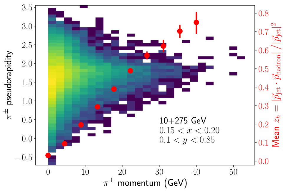
Figure 11 shows the momentum and pseudorapdity distribution of charged pions in jets for events with , as well as the average value sampled in each momentum interval. Positive particle identification of pions up to 40 GeV at 1.5–2.0 is required to reach . Smaller ranges yield smaller jet momentum and thus less stringent requirements.
V.4 Systematic uncertainties
Most sources of systematic uncertainties in jet measurements, including jet-energy scale (JES) and jet-energy resolution (JER) uncertainties, cancel in the spin-asymmetry ratios. Time drifts in the detectors response can be suppressed to a negligible level with the bunch-to-bunch control of the beam polarization pioneered at RHIC, which will transfer to EIC.
While the JES uncertainty does not affect the scale of the asymmetry, it affects the definition of (the jet momentum appears in the denominator) or (proportional to jet momentum), so it translates to a horizontal uncertainty in the differential asymmetry measurements. We show that a conservative estimate of 3 for the JES uncertainty would still allow us to sample the predicted -dependence of the Collins asymmetries shown in Figure 6 or the Sivers asymmetry shown in Figure 5.
While the asymmetry measurements have the potential to be very accurate, the unpolarized cross section measurement will be much more challenging due to the JES uncertainty. HERA experiments ultimately achieved a JES uncertainty of about 1% Newman:2013ada, but there are several challenges for the EIC. The accelerator design that leads to an improvement of the instantaneous luminosity compared to HERA requires focusing magnets closer to the interaction point. This limits the space for detectors, which will result in “thin” hadronic calorimeters that motivate the constant terms in Table 1; this will also lead to more difficult JES estimates.
While difficult, the measurement of the unpolarized cross sections is crucial to constrain nonperturbative aspects of TMD-evolution which is not only motivated by the need to understand the hadronization process itself but ultimately improves the accuracy of the extractions of the Sivers function Echevarria:2014xaa.
Estimations of the jet energy scale uncertainty are notoriously difficult and involve several studies that cover beam-test data, in-situ calibrations, and Monte-Carlo simulations (e.g. Ref. Khachatryan:2016kdb), which are outside the scope of this work.
Systematic uncertainties that do not cancel in the asymmetry ratio are the ones associated with the relative luminosity for each polarization state and the beam polarization. The relative luminosity uncertainty will be , as demonstrated at RHIC. The relative uncertainty on the hadron polarization is expected to be at the EIC. Given the absolute magnitude of the Sivers and Collins asymmetries we predict, neither of these uncertainties will be a limiting factor.
The systematic uncertainties associated with the underlying event, which were dominant at low in Sivers- and Collins-asymmetry studies at RHIC Abelev:2007ii; Adamczyk:2017wld, will be negligible given that high DIS is essentially free from ambiguities due to the beam-remnant (as illustrated in Figure 7).
VI Conclusions
We have presented predictions and projections for measurements of the Sivers asymmetry with electron-jet azimuthal correlations and the Collins asymmetry with hadron-in-jet measurements at the EIC. In particular, we have presented for the first time predictions for Collins asymmetries using hadrons inside jets and we argued that it will be a key channel to access quark transversity, Collins fragmentation functions, and to study their evolution.
We have explored the feasibility of these measurements based on fast simulations implemented with the Delphes package and found that the expected performance of a hermetic EIC detector with reasonable parameters is sufficient to perform these measurements. We have discussed detector requirements and suggested further studies to go along with dedicated detector simulations to inform the design of future EIC experiments, which we argue should include jet capabilities from day one.
While jet-based measurements of Sivers and transversity functions are powerful and novel ways to achieve some of the main scientific goals of the EIC, the potential of jets transcends these two examples. A promising case are novel jet substructure studies for TMD observables, which we leave for future work. This work represents a new direction for the rapidly emerging field of jet studies at the future EIC Arratia:2020azl; Arratia:2020ssx; Borsa:2020ulb; Peccini:2020tpj; Guzey:2020gkk; Guzey:2020zza; Kang:2020xyq; Arratia:2019vju; Page:2019gbf; Li:2020sru; Gutierrez-Reyes:2019vbx; Gutierrez-Reyes:2019msa; Zhang:2019toi; Aschenauer:2019uex; Hatta:2019ixj; Mantysaari:2019csc; DAlesio:2019qpk; Kishore:2019fzb; Kang:2019bpl; Roy:2019cux; Roy:2019hwr; Salazar:2019ncp; Gutierrez-Reyes:2018qez; Boughezal:2018azh; Klasen:2018gtb; Dumitru:2018kuw; Liu:2018trl; Zheng:2018ssm; Sievert:2018imd; Klasen:2017kwb; Hinderer:2017ntk; Chu:2017mnm; Aschenauer:2017jsk; Abelof:2016pby; Hatta:2016dxp; Dumitru:2016jku; Boer:2016fqd; Dumitru:2015gaa; Hinderer:2015hra; Altinoluk:2015dpi; Kang:2013nha; Pisano:2013cya; Kang:2012zr; Kang:2011jw; Boer:2010zf.
Code availability
The Delphes configuration file for the EIC general-purpose detector considered in this work can be found at: https://github.com/miguelignacio/delphes_EIC/blob/master/delphes_card_EIC.tcl
Acknowledgements
We thank Oleg Tsai for insightful discussions on calorimetry technology for EIC detectors. We thank Elke Aschenauer, Barbara Jacak, Kyle Lee, Brian Page and Feng Yuan for enlightening discussions about jet physics at the EIC and Anselm Vossen, Feng Yuan, Sean Preins, and Sebouh Paul for feedback on our manuscript. We thank the members of the EIC User Group for many insightful discussions during the Yellow Report activities. M.A and A.P. acknowledges support through DOE Contract No. DE-AC05-06OR23177 under which Jefferson Science Associates, LLC operates the Thomas Jefferson National Accelerator Facility. Z.K. is supported by the National Science Foundation under Grant No. PHY-1720486 and CAREER award PHY-1945471. A.P. is supported by the National Science Foundation under Grant No. PHY-2012002. F.R. is supported by LDRD funding from Berkeley Lab provided by the U.S. Department of Energy under Contract No. DE-AC02-05CH11231 as well as the National Science Foundation under Grant No. ACI-1550228.
Appendix A Relevant perturbative results at one-loop
Here we summarize the different functions that appear in the factorization formulas in Eqs. (II.1) and (II.2). We work in Fourier-transform space where all the associated renormalization group equations are multiplicative. They can be derived from the fixed-order result along with the relevant anomalous dimensions. In the unpolarized case we have
| (22) | ||||
| (23) | ||||
| (24) |
where . The factorization here holds for . Note that all terms cancel at fixed order.
The unpolarized TMD PDF and FF can be matched onto the collinear PDFs at low values of as
| (25) | ||||
| (26) |
where according to Ref. Meng:1995yn; Nadolsky:1999kb; Koike:2006fn; Kang:2015msa,
| (27) | ||||
| (28) | ||||
| (29) | ||||
| (30) |
with the usual splitting functions and given by
| (31) | ||||
| (32) |
The energy evolution of TMDs from the scale to the scale is encoded in the exponential factor, , with the Sudakov-like form factor, the perturbative part of which can be written as
| (33) |
Here the coefficients and can be expanded as a perturbative series , . In our calculations, we take into account , and to achieve NLL accuracy. Because this part is spin-independent, these coefficients are the same for the polarized and unpolarized cross sections Collins:1984kg and are given by Kang:2011mr; Aybat:2011zv; Echevarria:2012pw; Collins:1984kg; Qiu:2000ga; Landry:2002ix:
| (34) |
In order to avoid the Landau pole , we use the standard -prescription that introduces a cutoff value and allows for a smooth transition from the perturbative to the nonperturbative region,
| (35) |
where is a parameter of the prescription. From the above definition, is always in the perturbative region where was chosen Kang:2015msa to be 1.5 GeV-1. When is introduced in the Sudakov form factor, the total Sudakov-like form factor can be written as the sumof the perturbatively calculable part and a nonperturbative contribution
| (36) |
where is defined as the difference between the original form factor and the perturbative one. Eventually, we have
| (37) | ||||
| (38) |
In our calculations we use the prescriptions for the nonperturbative functions and the treatment of the Collins fragmentation and Sivers functions of Refs. Kang:2015msa; Echevarria:2014xaa.
Bibliography
- (1) A. J. Larkoski, I. Moult, and B. Nachman, “Jet Substructure at the Large Hadron Collider: A Review of Recent Advances in Theory and Machine Learning,” Phys. Rept. 841 (2020) 1–63, arXiv:1709.04464 [hep-ph].
- (2) D. Boer and C. Pisano, “Impact of gluon polarization on Higgs boson plus jet production at the LHC,” Phys. Rev. D 91 no. 7, (2015) 074024, arXiv:1412.5556 [hep-ph].
- (3) ATLAS Collaboration, G. Aad et al., “Measurement of the jet fragmentation function and transverse profile in proton-proton collisions at a center-of-mass energy of 7 TeV with the ATLAS detector,” Eur. Phys. J. C 71 (2011) 1795, arXiv:1109.5816 [hep-ex].
- (4) LHCb Collaboration, R. Aaij et al., “Measurement of charged hadron production in -tagged jets in proton-proton collisions at TeV,” Phys. Rev. Lett. 123 no. 23, (2019) 232001, arXiv:1904.08878 [hep-ex].
- (5) Z.-B. Kang, K. Lee, J. Terry, and H. Xing, “Jet fragmentation functions for -tagged jets,” Phys. Lett. B 798 (2019) 134978, arXiv:1906.07187 [hep-ph].
- (6) D. Gutierrez-Reyes, I. Scimemi, W. J. Waalewijn, and L. Zoppi, “Transverse momentum dependent distributions with jets,” Phys. Rev. Lett. 121 no. 16, (2018) 162001, arXiv:1807.07573 [hep-ph].
- (7) D. Gutierrez-Reyes, I. Scimemi, W. J. Waalewijn, and L. Zoppi, “Transverse momentum dependent distributions in and semi-inclusive deep-inelastic scattering using jets,” JHEP 10 (2019) 031, arXiv:1904.04259 [hep-ph].
- (8) X. Liu, F. Ringer, W. Vogelsang, and F. Yuan, “Lepton-jet Correlations in Deep Inelastic Scattering at the Electron-Ion Collider,” Phys. Rev. Lett. 122 no. 19, (2019) 192003, arXiv:1812.08077 [hep-ph].
- (9) Z.-B. Kang, K. Lee, and F. Zhao, “Polarized jet fragmentation functions,” arXiv:2005.02398 [hep-ph].
- (10) D. Boer and W. Vogelsang, “Asymmetric jet correlations in p p uparrow scattering,” Phys. Rev. D 69 (2004) 094025, arXiv:hep-ph/0312320.
- (11) STAR Collaboration, B. I. Abelev et al., “Measurement of transverse single-spin asymmetries for di-jet production in proton-proton collisions at s**(1/2) = 200-GeV,” Phys. Rev. Lett. 99 (2007) 142003, arXiv:0705.4629 [hep-ex].
- (12) C. Bomhof, P. Mulders, W. Vogelsang, and F. Yuan, “Single-Transverse Spin Asymmetry in Dijet Correlations at Hadron Colliders,” Phys. Rev. D 75 (2007) 074019, arXiv:hep-ph/0701277.
- (13) STAR Collaboration, L. Adamczyk et al., “Azimuthal transverse single-spin asymmetries of inclusive jets and charged pions within jets from polarized-proton collisions at GeV,” Phys. Rev. D97 no. 3, (2018) 032004, arXiv:1708.07080 [hep-ex].
- (14) Z.-B. Kang, A. Prokudin, F. Ringer, and F. Yuan, “Collins azimuthal asymmetries of hadron production inside jets,” Phys. Lett. B774 (2017) 635–642, arXiv:1707.00913 [hep-ph].
- (15) U. D’Alesio, F. Murgia, and C. Pisano, “Testing the universality of the Collins function in pion-jet production at RHIC,” Phys. Lett. B 773 (2017) 300–306, arXiv:1707.00914 [hep-ph].
- (16) A. Accardi et al., “Electron Ion Collider: The Next QCD Frontier,” Eur. Phys. J. A52 no. 9, (2016) 268, arXiv:1212.1701 [nucl-ex].
- (17) M. Boglione, J. Collins, L. Gamberg, J. O. Gonzalez-Hernandez, T. C. Rogers, and N. Sato, “Kinematics of Current Region Fragmentation in Semi-Inclusive Deeply Inelastic Scattering,” Phys. Lett. B766 (2017) 245–253, arXiv:1611.10329 [hep-ph].
- (18) M. Boglione, A. Dotson, L. Gamberg, S. Gordon, J. O. Gonzalez-Hernandez, A. Prokudin, T. C. Rogers, and N. Sato, “Mapping the Kinematical Regimes of Semi-Inclusive Deep Inelastic Scattering,” JHEP 10 (2019) 122, arXiv:1904.12882 [hep-ph].
- (19) E. C. Aschenauer, I. Borsa, R. Sassot, and C. Van Hulse, “Semi-inclusive Deep-Inelastic Scattering, Parton Distributions and Fragmentation Functions at a Future Electron-Ion Collider,” Phys. Rev. D99 no. 9, (2019) 094004, arXiv:1902.10663 [hep-ph].
- (20) M. Arratia, Y. Song, F. Ringer, and B. Jacak, “Jets as precision probes in electron-nucleus collisions at the Electron-Ion Collider,” Phys. Rev. C 101 (2020) 065204, arXiv:1912.05931 [nucl-ex].
- (21) M. G. Buffing, Z.-B. Kang, K. Lee, and X. Liu, “A transverse momentum dependent framework for back-to-back photon+jet production,” arXiv:1812.07549 [hep-ph].
- (22) R. Bain, Y. Makris, and T. Mehen, “Transverse Momentum Dependent Fragmenting Jet Functions with Applications to Quarkonium Production,” JHEP 11 (2016) 144, arXiv:1610.06508 [hep-ph].
- (23) Z.-B. Kang, X. Liu, F. Ringer, and H. Xing, “The transverse momentum distribution of hadrons within jets,” JHEP 11 (2017) 068, arXiv:1705.08443 [hep-ph].
- (24) P. Sun, C. P. Yuan, and F. Yuan, “Transverse Momentum Resummation for Dijet Correlation in Hadronic Collisions,” Phys. Rev. D 92 no. 9, (2015) 094007, arXiv:1506.06170 [hep-ph].
- (25) P. Sun, B. Yan, C.-P. Yuan, and F. Yuan, “Resummation of High Order Corrections in Boson Plus Jet Production at the LHC,” Phys. Rev. D 100 no. 5, (2019) 054032, arXiv:1810.03804 [hep-ph].
- (26) D. Bertolini, T. Chan, and J. Thaler, “Jet Observables Without Jet Algorithms,” JHEP 04 (2014) 013, arXiv:1310.7584 [hep-ph].
- (27) Y.-T. Chien, R. Rahn, S. S. van Velzen, D. Y. Shao, W. J. Waalewijn, and B. Wu, “Azimuthal angle for boson-jet production in the back-to-back limit,” arXiv:2005.12279 [hep-ph].
- (28) M. Dasgupta, A. Fregoso, S. Marzani, and G. P. Salam, “Towards an understanding of jet substructure,” JHEP 09 (2013) 029, arXiv:1307.0007 [hep-ph].
- (29) A. J. Larkoski, S. Marzani, G. Soyez, and J. Thaler, “Soft Drop,” JHEP 05 (2014) 146, arXiv:1402.2657 [hep-ph].
- (30) D. Gutierrez-Reyes, Y. Makris, V. Vaidya, I. Scimemi, and L. Zoppi, “Probing Transverse-Momentum Distributions With Groomed Jets,” JHEP 08 (2019) 161, arXiv:1907.05896 [hep-ph].
- (31) Y. Makris, D. Neill, and V. Vaidya, “Probing Transverse-Momentum Dependent Evolution With Groomed Jets,” JHEP 07 (2018) 167, arXiv:1712.07653 [hep-ph].
- (32) P. Cal, D. Neill, F. Ringer, and W. J. Waalewijn, “Calculating the angle between jet axes,” arXiv:1911.06840 [hep-ph].
- (33) D. Neill, I. Scimemi, and W. J. Waalewijn, “Jet axes and universal transverse-momentum-dependent fragmentation,” JHEP 04 (2017) 020, arXiv:1612.04817 [hep-ph].
- (34) D. Neill, A. Papaefstathiou, W. J. Waalewijn, and L. Zoppi, “Phenomenology with a recoil-free jet axis: TMD fragmentation and the jet shape,” JHEP 01 (2019) 067, arXiv:1810.12915 [hep-ph].
- (35) F. Yuan, “Azimuthal asymmetric distribution of hadrons inside a jet at hadron collider,” Phys. Rev. Lett. 100 (2008) 032003, arXiv:0709.3272 [hep-ph].
- (36) E.-C. Aschenauer et al., “The RHIC Cold QCD Plan for 2017 to 2023: A Portal to the EIC,” arXiv:1602.03922 [nucl-ex].
- (37) M. Anselmino et al., “Transverse Momentum Dependent Parton Distribution/Fragmentation Functions at an Electron-Ion Collider,” Eur. Phys. J. A47 (2011) 35, arXiv:1101.4199 [hep-ex].
- (38) H. H. Matevosyan, A. Kotzinian, E.-C. Aschenauer, H. Avakian, and A. W. Thomas, “Predictions for Sivers single spin asymmetries in one- and two-hadron electroproduction at CLAS12 and EIC,” Phys. Rev. D92 no. 5, (2015) 054028, arXiv:1502.02669 [hep-ph].
- (39) L. Zheng, E. C. Aschenauer, J. H. Lee, B.-W. Xiao, and Z.-B. Yin, “Accessing the gluon Sivers function at a future electron-ion collider,” Phys. Rev. D98 no. 3, (2018) 034011, arXiv:1805.05290 [hep-ph].
- (40) M. Cacciari, G. P. Salam, and G. Soyez, “The anti- jet clustering algorithm,” JHEP 04 (2008) 063, arXiv:0802.1189 [hep-ph].
- (41) J. Collins, Foundations of perturbative QCD, vol. 32. Cambridge University Press, 11, 2013.
- (42) M. Dasgupta and G. Salam, “Resummation of nonglobal QCD observables,” Phys. Lett. B 512 (2001) 323–330, arXiv:hep-ph/0104277.
- (43) A. Banfi and M. Dasgupta, “Dijet rates with symmetric E(t) cuts,” JHEP 01 (2004) 027, arXiv:hep-ph/0312108.
- (44) Y.-T. Chien, D. Y. Shao, and B. Wu, “Resummation of Boson-Jet Correlation at Hadron Colliders,” JHEP 11 (2019) 025, arXiv:1905.01335 [hep-ph].
- (45) T. Kaufmann, A. Mukherjee, and W. Vogelsang, “Hadron Fragmentation Inside Jets in Hadronic Collisions,” Phys. Rev. D 92 no. 5, (2015) 054015, arXiv:1506.01415 [hep-ph]. [Erratum: Phys.Rev.D 101, 079901 (2020)].
- (46) Z.-B. Kang, F. Ringer, and I. Vitev, “Jet substructure using semi-inclusive jet functions in SCET,” JHEP 11 (2016) 155, arXiv:1606.07063 [hep-ph].
- (47) S. D. Ellis, C. K. Vermilion, J. R. Walsh, A. Hornig, and C. Lee, “Jet Shapes and Jet Algorithms in SCET,” JHEP 11 (2010) 101, arXiv:1001.0014 [hep-ph].
- (48) M. Procura and I. W. Stewart, “Quark Fragmentation within an Identified Jet,” Phys. Rev. D 81 (2010) 074009, arXiv:0911.4980 [hep-ph]. [Erratum: Phys.Rev.D 83, 039902 (2011)].
- (49) T. Sjostrand, S. Mrenna, and P. Z. Skands, “A Brief Introduction to PYTHIA 8.1,” Comput. Phys. Commun. 178 (2008) 852–867, arXiv:0710.3820 [hep-ph].
- (50) S. Höche and S. Prestel, “The midpoint between dipole and parton showers,” Eur. Phys. J. C75 no. 9, (2015) 461, arXiv:1506.05057 [hep-ph].
- (51) BNL, “An electron-ion collider study.” https://wiki.bnl.gov/eic/upload/EIC.Design.Study.pdf, January, 2020.
- (52) G. Abelof, R. Boughezal, X. Liu, and F. Petriello, “Single-inclusive jet production in electron–nucleon collisions through next-to-next-to-leading order in perturbative QCD,” Phys. Lett. B763 (2016) 52–59, arXiv:1607.04921 [hep-ph].
- (53) F. Petriello. Personal communication.
- (54) B. Jager, “Photoproduction of single inclusive jets at future ep colliders in next-to-leading order QCD,” Phys. Rev. D 78 (2008) 034017, arXiv:0807.0066 [hep-ph].
- (55) E.-C. Aschenauer, K. Lee, B. Page, and F. Ringer, “Jet angularities in photoproduction at the Electron-Ion Collider,” Phys. Rev. D 101 no. 5, (2020) 054028, arXiv:1910.11460 [hep-ph].
- (56) Z.-B. Kang, A. Metz, J.-W. Qiu, and J. Zhou, “Exploring the structure of the proton through polarization observables in ,” Phys. Rev. D 84 (2011) 034046, arXiv:1106.3514 [hep-ph].
- (57) P. Hinderer, M. Schlegel, and W. Vogelsang, “Single-Inclusive Production of Hadrons and Jets in Lepton-Nucleon Scattering at NLO,” Phys. Rev. D 92 no. 1, (2015) 014001, arXiv:1505.06415 [hep-ph]. [Erratum: Phys.Rev.D 93, 119903 (2016)].
- (58) M. Cacciari, G. P. Salam, and G. Soyez, “FastJet User Manual,” Eur. Phys. J. C72 (2012) 1896, arXiv:1111.6097 [hep-ph].
- (59) P. Newman and M. Wing, “The Hadronic Final State at HERA,” Rev. Mod. Phys. 86 no. 3, (2014) 1037, arXiv:1308.3368 [hep-ex].
- (60) D. Boer, P. J. Mulders, and C. Pisano, “Dijet imbalance in hadronic collisions,” Phys. Rev. D 80 (2009) 094017, arXiv:0909.4652 [hep-ph].
- (61) M. Anselmino, A. Mukherjee, and A. Vossen, “Transverse spin effects in hard semi-inclusive collisions,” arXiv:2001.05415 [hep-ex].
- (62) D. de Florian, R. Sassot, and M. Stratmann, “Global analysis of fragmentation functions for pions and kaons and their uncertainties,” Phys. Rev. D 75 (2007) 114010, arXiv:hep-ph/0703242.
- (63) Z.-B. Kang, A. Prokudin, P. Sun, and F. Yuan, “Extraction of Quark Transversity Distribution and Collins Fragmentation Functions with QCD Evolution,” Phys. Rev. D 93 no. 1, (2016) 014009, arXiv:1505.05589 [hep-ph].
- (64) M. G. Echevarria, A. Idilbi, Z.-B. Kang, and I. Vitev, “QCD Evolution of the Sivers Asymmetry,” Phys. Rev. D 89 (2014) 074013, arXiv:1401.5078 [hep-ph].
- (65) A. Bacchetta, F. Delcarro, C. Pisano, and M. Radici, “The three-dimensional distribution of quarks in momentum space,” arXiv:2004.14278 [hep-ph].
- (66) S. J. Brodsky, D. S. Hwang, and I. Schmidt, “Final state interactions and single spin asymmetries in semiinclusive deep inelastic scattering,” Phys. Lett. B530 (2002) 99–107, arXiv:hep-ph/0201296 [hep-ph].
- (67) J. C. Collins, “Leading twist single transverse-spin asymmetries: Drell-Yan and deep inelastic scattering,” Phys. Lett. B 536 (2002) 43–48, arXiv:hep-ph/0204004.
- (68) D. Boer, P. Mulders, and F. Pijlman, “Universality of T odd effects in single spin and azimuthal asymmetries,” Nucl. Phys. B 667 (2003) 201–241, arXiv:hep-ph/0303034.
- (69) SoLID Collaboration, J. P. Chen, H. Gao, T. K. Hemmick, Z. E. Meziani, and P. A. Souder, “A White Paper on SoLID (Solenoidal Large Intensity Device),” arXiv:1409.7741 [nucl-ex].
- (70) E.-C. Aschenauer et al., “The RHIC SPIN Program: Achievements and Future Opportunities,” arXiv:1501.01220 [nucl-ex].
- (71) Z. Ye, N. Sato, K. Allada, T. Liu, J.-P. Chen, H. Gao, Z.-B. Kang, A. Prokudin, P. Sun, and F. Yuan, “Unveiling the nucleon tensor charge at Jefferson Lab: A study of the SoLID case,” Phys. Lett. B767 (2017) 91–98, arXiv:1609.02449 [hep-ph].
- (72) E. A. et al., “Electron-ion collider detector requirements and r&d handbook.” http://www.eicug.org/web/sites/default/files/EIC_HANDBOOK_v1.2.pdf, February, 2020.
- (73) DELPHES 3 Collaboration, J. de Favereau, C. Delaere, P. Demin, A. Giammanco, V. Lemaître, A. Mertens, and M. Selvaggi, “DELPHES 3, A modular framework for fast simulation of a generic collider experiment,” JHEP 02 (2014) 057, arXiv:1307.6346 [hep-ex].
- (74) M. Arratia, Y. Furletova, T. Hobbs, F. Olness, and S. J. Sekula, “Charm jets as a probe for strangeness at the future Electron-Ion Collider,” arXiv:2006.12520 [hep-ph].
- (75) GEANT4 Collaboration, S. Agostinelli et al., “GEANT4: A Simulation toolkit,” Nucl. Instrum. Meth. A 506 (2003) 250–303.
- (76) sPHENIX Collaboration, C. A. Aidala et al., “Design and Beam Test Results for the sPHENIX Electromagnetic and Hadronic Calorimeter Prototypes,” IEEE Trans. Nucl. Sci. 65 no. 12, (2018) 2901–2919, arXiv:1704.01461 [physics.ins-det].
- (77) O. D. Tsai, E. Aschenauer, W. Christie, L. E. Dunkelberger, S. Fazio, C. A. Gagliardi, S. Heppelmann, H. Z. Huang, W. W. Jacobs, G. Igo, A. Kisilev, K. Landry, X. Liu, M. M. Mondal, Y. X. Pan, M. Sergeeva, N. Shah, E. Sichtermann, S. Trentalange, G. Visser, and S. Wissink, “Development of a forward calorimeter system for the STAR experiment,” Journal of Physics: Conference Series 587 (Feb, 2015) 012053. https://doi.org/10.1088%2F1742-6596%2F587%2F1%2F012053.
- (78) PHENIX Collaboration, A. Adare et al., “An Upgrade Proposal from the PHENIX Collaboration,” arXiv:1501.06197 [nucl-ex].
- (79) B. Page, X. Chu, and E. Aschenauer, “Experimental Aspects of Jet Physics at a Future EIC,” Phys. Rev. D 101 no. 7, (2020) 072003, arXiv:1911.00657 [hep-ph].
- (80) H.-M. Chang, M. Procura, J. Thaler, and W. J. Waalewijn, “Calculating Track Thrust with Track Functions,” Phys. Rev. D 88 (2013) 034030, arXiv:1306.6630 [hep-ph].
- (81) H.-M. Chang, M. Procura, J. Thaler, and W. J. Waalewijn, “Calculating Track-Based Observables for the LHC,” Phys. Rev. Lett. 111 (2013) 102002, arXiv:1303.6637 [hep-ph].
- (82) J. K. Adkins, Studying Transverse Momentum Dependent Distributions in Polarized Proton Collisions via Azimuthal Single Spin Asymmetries of Charged Pions in Jets. PhD thesis, Kentucky U., 2015. arXiv:1907.11233 [hep-ex].
- (83) Y. Pan, Transverse single spin asymmetry measurements at STAR. PhD thesis, University of California, Los Angeles, 2015.
- (84) CMS Collaboration, V. Khachatryan et al., “Jet energy scale and resolution in the CMS experiment in pp collisions at 8 TeV,” JINST 12 no. 02, (2017) P02014, arXiv:1607.03663 [hep-ex].
- (85) M. Arratia, Y. Makris, D. Neill, F. Ringer, and N. Sato, “Asymmetric jet clustering in deep-inelastic scattering,” arXiv:2006.10751 [hep-ph].
- (86) I. Borsa, D. de Florian, and I. Pedron, “Jet production in Polarized DIS at NNLO,” arXiv:2005.10705 [hep-ph].
- (87) G. Peccini, L. Moriggi, and M. Machado, “Investigating the diffractive gluon jet production in lepton-ion collisions,” arXiv:2003.13882 [hep-ph].
- (88) V. Guzey and M. Klasen, “Diffractive dijet photoproduction at the EIC,” JHEP 05 (2020) 074, arXiv:2004.06972 [hep-ph].
- (89) V. Guzey and M. Klasen, “NLO QCD predictions for dijet photoproduction in lepton-nucleus scattering at the EIC, LHeC, HE-LHeC, and FCC,” arXiv:2003.09129 [hep-ph].
- (90) X. Li et al., “A New Heavy Flavor Program for the Future Electron-Ion Collider,” EPJ Web Conf. 235 (2020) 04002, arXiv:2002.05880 [nucl-ex].
- (91) Y.-Y. Zhang, G.-Y. Qin, and X.-N. Wang, “Parton energy loss in generalized high twist approach,” Phys. Rev. D 100 no. 7, (2019) 074031, arXiv:1905.12699 [hep-ph].
- (92) Y. Hatta, N. Mueller, T. Ueda, and F. Yuan, “QCD Resummation in Hard Diffractive Dijet Production at the Electron-Ion Collider,” arXiv:1907.09491 [hep-ph].
- (93) H. Mäntysaari, N. Mueller, and B. Schenke, “Diffractive Dijet Production and Wigner Distributions from the Color Glass Condensate,” Phys. Rev. D99 no. 7, (2019) 074004, arXiv:1902.05087 [hep-ph].
- (94) U. D’Alesio, F. Murgia, C. Pisano, and P. Taels, “Azimuthal asymmetries in semi-inclusive production at an EIC,” arXiv:1908.00446 [hep-ph].
- (95) R. Kishore, A. Mukherjee, and S. Rajesh, “Sivers Asymmetry in Photoproduction of and Jet at the EIC,” arXiv:1908.03698 [hep-ph].
- (96) D. Kang and T. Maji, “Toward precision jet event shape for future Electron-Ion Collider,” PoS LC2019 (2019) 061, arXiv:1912.10656 [hep-ph].
- (97) K. Roy and R. Venugopalan, “Extracting many-body correlators of saturated gluons with precision from inclusive photon+dijet final states in deeply inelastic scattering,” Phys. Rev. D 101 no. 7, (2020) 071505, arXiv:1911.04519 [hep-ph].
- (98) K. Roy and R. Venugopalan, “NLO impact factor for inclusive photondijet production in DIS at small ,” arXiv:1911.04530 [hep-ph].
- (99) F. Salazar and B. Schenke, “Diffractive dijet production in impact parameter dependent saturation models,” Phys. Rev. D100 no. 3, (2019) 034007, arXiv:1905.03763 [hep-ph].
- (100) R. Boughezal, F. Petriello, and H. Xing, “Inclusive jet production as a probe of polarized parton distribution functions at a future EIC,” Phys. Rev. D98 no. 5, (2018) 054031, arXiv:1806.07311 [hep-ph].
- (101) M. Klasen and K. Kovařík, “Nuclear parton density functions from dijet photoproduction at the EIC,” Phys. Rev. D97 no. 11, (2018) 114013, arXiv:1803.10985 [hep-ph].
- (102) A. Dumitru, V. Skokov, and T. Ullrich, “Measuring the Weizsäcker-Williams distribution of linearly polarized gluons at an electron-ion collider through dijet azimuthal asymmetries,” Phys. Rev. C99 no. 1, (2019) 015204, arXiv:1809.02615 [hep-ph].
- (103) L. Zheng, E. Aschenauer, J. Lee, B.-W. Xiao, and Z.-B. Yin, “Accessing the gluon Sivers function at a future electron-ion collider,” Phys. Rev. D 98 no. 3, (2018) 034011, arXiv:1805.05290 [hep-ph].
- (104) M. D. Sievert and I. Vitev, “Quark branching in QCD matter to any order in opacity beyond the soft gluon emission limit,” Phys. Rev. D98 no. 9, (2018) 094010, arXiv:1807.03799 [hep-ph].
- (105) M. Klasen, K. Kovarik, and J. Potthoff, “Nuclear parton density functions from jet production in DIS at an EIC,” Phys. Rev. D95 no. 9, (2017) 094013, arXiv:1703.02864 [hep-ph].
- (106) P. Hinderer, M. Schlegel, and W. Vogelsang, “Double-Longitudinal Spin Asymmetry in Single-Inclusive Lepton Scattering at NLO,” Phys. Rev. D96 no. 1, (2017) 014002, arXiv:1703.10872 [hep-ph].
- (107) X. Chu, E.-C. Aschenauer, J.-H. Lee, and L. Zheng, “Photon structure studied at an Electron Ion Collider,” Phys. Rev. D96 no. 7, (2017) 074035, arXiv:1705.08831 [nucl-ex].
- (108) E. Aschenauer, S. Fazio, J. Lee, H. Mantysaari, B. Page, B. Schenke, T. Ullrich, R. Venugopalan, and P. Zurita, “The electron–ion collider: assessing the energy dependence of key measurements,” Rept. Prog. Phys. 82 no. 2, (2019) 024301, arXiv:1708.01527 [nucl-ex].
- (109) Y. Hatta, B.-W. Xiao, and F. Yuan, “Probing the Small-x Gluon Tomography in Correlated Hard Diffractive Dijet Production in Deep Inelastic Scattering,” Phys. Rev. Lett. 116 no. 20, (2016) 202301, arXiv:1601.01585 [hep-ph].
- (110) A. Dumitru and V. Skokov, “ azimuthal anisotropy in small- DIS dijet production beyond the leading power TMD limit,” Phys. Rev. D94 no. 1, (2016) 014030, arXiv:1605.02739 [hep-ph].
- (111) D. Boer, P. J. Mulders, C. Pisano, and J. Zhou, “Asymmetries in Heavy Quark Pair and Dijet Production at an EIC,” JHEP 08 (2016) 001, arXiv:1605.07934 [hep-ph].
- (112) A. Dumitru, T. Lappi, and V. Skokov, “Distribution of Linearly Polarized Gluons and Elliptic Azimuthal Anisotropy in Deep Inelastic Scattering Dijet Production at High Energy,” Phys. Rev. Lett. 115 no. 25, (2015) 252301, arXiv:1508.04438 [hep-ph].
- (113) T. Altinoluk, N. Armesto, G. Beuf, and A. H. Rezaeian, “Diffractive Dijet Production in Deep Inelastic Scattering and Photon-Hadron Collisions in the Color Glass Condensate,” Phys. Lett. B758 (2016) 373–383, arXiv:1511.07452 [hep-ph].
- (114) D. Kang, C. Lee, and I. W. Stewart, “Using 1-Jettiness to Measure 2 Jets in DIS 3 Ways,” Phys. Rev. D88 (2013) 054004, arXiv:1303.6952 [hep-ph].
- (115) C. Pisano, D. Boer, S. J. Brodsky, M. G. A. Buffing, and P. J. Mulders, “Linear polarization of gluons and photons in unpolarized collider experiments,” JHEP 10 (2013) 024, arXiv:1307.3417 [hep-ph].
- (116) Z.-B. Kang, S. Mantry, and J.-W. Qiu, “N-Jettiness as a Probe of Nuclear Dynamics,” Phys. Rev. D86 (2012) 114011, arXiv:1204.5469 [hep-ph].
- (117) D. Boer, S. J. Brodsky, P. J. Mulders, and C. Pisano, “Direct Probes of Linearly Polarized Gluons inside Unpolarized Hadrons,” Phys. Rev. Lett. 106 (2011) 132001, arXiv:1011.4225 [hep-ph].
- (118) R. Meng, F. I. Olness, and D. E. Soper, “Semiinclusive deeply inelastic scattering at small q(T),” Phys. Rev. D 54 (1996) 1919–1935, arXiv:hep-ph/9511311.
- (119) P. M. Nadolsky, D. Stump, and C. Yuan, “Semiinclusive hadron production at HERA: The Effect of QCD gluon resummation,” Phys. Rev. D 61 (2000) 014003, arXiv:hep-ph/9906280. [Erratum: Phys.Rev.D 64, 059903 (2001)].
- (120) Y. Koike, J. Nagashima, and W. Vogelsang, “Resummation for polarized semi-inclusive deep-inelastic scattering at small transverse momentum,” Nucl. Phys. B 744 (2006) 59–79, arXiv:hep-ph/0602188.
- (121) J. C. Collins, D. E. Soper, and G. F. Sterman, “Transverse Momentum Distribution in Drell-Yan Pair and W and Z Boson Production,” Nucl. Phys. B 250 (1985) 199–224.
- (122) Z.-B. Kang, B.-W. Xiao, and F. Yuan, “QCD Resummation for Single Spin Asymmetries,” Phys. Rev. Lett. 107 (2011) 152002, arXiv:1106.0266 [hep-ph].
- (123) S. Aybat and T. C. Rogers, “TMD Parton Distribution and Fragmentation Functions with QCD Evolution,” Phys. Rev. D 83 (2011) 114042, arXiv:1101.5057 [hep-ph].
- (124) M. G. Echevarria, A. Idilbi, A. Schäfer, and I. Scimemi, “Model-Independent Evolution of Transverse Momentum Dependent Distribution Functions (TMDs) at NNLL,” Eur. Phys. J. C 73 no. 12, (2013) 2636, arXiv:1208.1281 [hep-ph].
- (125) J.-w. Qiu and X.-f. Zhang, “QCD prediction for heavy boson transverse momentum distributions,” Phys. Rev. Lett. 86 (2001) 2724–2727, arXiv:hep-ph/0012058.
- (126) F. Landry, R. Brock, P. M. Nadolsky, and C. Yuan, “Tevatron Run-1 boson data and Collins-Soper-Sterman resummation formalism,” Phys. Rev. D 67 (2003) 073016, arXiv:hep-ph/0212159.
*