6D SCFTs, 4D SCFTs,
Conformal Matter, and Spin Chains

One of the welcome surprises from string theory is the prediction of entirely new classes of quantum field theories, such as interacting conformal fixed points in six spacetime dimensions (see e.g. [1, 2, 3]). A remarkable feature of all higher-dimensional fixed points is that they are “non-Lagrangian” in the sense that they cannot be constructed from perturbations of a Gaussian fixed point produced from free fields. By the same token, this significantly complicates the study of such theories since many textbook techniques based on perturbation theory are seemingly inapplicable.

In spite of these difficulties, the mere existence of higher-dimensional fixed points provides a useful tool in the study of lower-dimensional systems. For example, compactifications of 6D superconformal field theories (6D SCFTs) produces a wealth of new sorts of lower-dimensional quantum field theories. Additionally, dualities of known 4D quantum field theories can be understood in terms of suitable compactifications of 6D SCFTs (see e.g. [4, 5, 6, 7]). Clearly, it would be desirable to better understand the structure of such systems, both as a subject of interest in its own right, and also in terms of possible lower-dimensional applications.

One of the original ways to construct and study examples of such theories has been through string compactification on singular geometries [1]. Recent progress includes a classification of all singular F-theory backgrounds which can generate a 6D SCFT [8, 9] (see also [10, 11] and [12] for a review). A perhaps surprising outcome of this analysis is that on a partially resolved phase of the singular geometry known as the partial tensor branch, all known theories have a quiver-like structure which typically consists of a single spine of ADE gauge group factors which are connected by 6D conformal matter (see figure 1 for a depiction). The geometric realization provides direct access to the moduli space of these theories.

Complementary methods of study for 6D SCFTs include the use of the conformal bootstrap [13, 14, 15], as well as the construction and study of holographic duals (see e.g. [16, 17, 18, 19, 20]). Both have proven useful in extracting some information on the operator content of 6D SCFTs, though it is fair to say that a more complete understanding is still to be achieved. In particular, extracting the explicit spectrum of operators and scaling dimensions in 6D SCFTs has proven to be quite challenging.

Our aim in this paper will be to better understand the operator content of 6D SCFTs, as well as their 4D descendants obtained from dimensional reduction. We present evidence that in the limit where the length of a generalized quiver becomes sufficiently long, there is a subsector of “nearly-protected” operators which have large R-charge $J$. In a sense we make precise, we find that the scaling dimension for these operators can be organized as a perturbation series above a bare scaling dimension $\Delta_{0}$:

$$\Delta=\Delta_{0}+\frac{\alpha}{J^{2}}+\mathcal{O}(J^{-3}),$$

(1.1)

that is, we identify a perturbative expansion in large R-charge, and use it to extract details of operator mixing in the 6D SCFT. This is very much in the spirit of lower-dimensional examples where large R-charge limits were fruitfully applied, as in reference [21], as well as [22].

The operating assumption we make throughout this paper is that the 6D conformal matter appearing as links in the generalized quiver description of all 6D SCFTs can be used to define a class of operators in the 6D SCFT which trigger Higgs branch deformations. Indeed, this picture was used in [18, 23] to show that complex structure deformations of the F-theory background can be interpreted as vacuum expectation values (vevs) for operators in the accompanying SCFT. For the most part, these rules are quite similar to Higgsing involving weakly coupled hypermultiplets [17, 18, 23, 24, 25, 26], though it was also observed in [23] that the scaling dimensions for these operators are always significantly higher than that of a weakly coupled hypermultiplet.

By assumption, giving a vev to one such operator triggers a Higgs branch deformation, and on the Higgs branch, we can study the resulting Nambu–Goldstone bosons. These bosons transform in a spin $s$ representation of $SU(2)_{\mathcal{R}}$, as dictated by the scaling dimension of the conformal matter operators. In a generalized quiver with $N$ gauge group factors $G_{i}$, and flavor symmetries $G_{0}$ and $G_{N+1}$ denoted via square brackets, which has the form:

$$[G_{0}]-G_{1}-\dots-G_{N}-[G_{N+1}]\,,$$

(1.2)

we can, on the Higgs branch, visualize each link as a collection of Goldstone modes in a representation of $SU(2)_{\mathcal{R}}$ R-symmetry. For the bifundamental between $G_{i}\times G_{i+1}$, we will typically label these modes as $X^{(m_{i})}_{i}$ for $-s\leq m_{i}\leq s$, and for the highest, respectively lowest, weight we shall use the simplified notation $X_{i}$, respectively $Y_{i}^{{\dagger}}$.

Assuming the existence of these operators, we get a tremendous amount of mileage in building gauge invariant combinations which survive as we move to the origin of the tensor branch. As an example, we can construct the gauge invariant composite bifundamental operator:

$$\mathcal{O}_{\mathrm{pure}}=\sqrt{\mathcal{Z}_{N}}X_{0}...X_{N}\,,$$

(1.3)

where the normalization factor, $\mathcal{Z}_{N}$, depends on the number of fields and gauge groups, and is chosen such that the two-point function of $\mathcal{O}_{\text{pure}}$ has coefficient one. Similar protected operators were considered in [20].

Owing to the R-symmetry and flavor symmetry content of $\mathcal{O}_{\mathrm{pure}}$, we expect it to have a protected scaling dimension proportional to $(N+1)$, the number of generalized bifundamentals appearing in the product. We can also consider descending to lower weight states for each $X_{i}$. Doing so we get gauge invariant composite operators such as:

$$\mathcal{O}_{m_{0},...,m_{N}}=\sqrt{\mathcal{Z}_{N}}X^{(m_{0})}_{0}...X^{(m_{N})}_{N},$$

(1.4)

which has the structure of a 1D spin chain with each site a spin $s$ representation of $SU(2)_{\mathcal{R}}$. While the highest weight state is $1/2$-BPS and protected, in 6D and for the analogous operators in 4D, we expect there is operator mixing for other values of the $m_{i}$. This leads to a correspondence between states of a spin chain and local operators:

$$\left|m_{0},...,m_{N}\right>\longleftrightarrow\mathcal{O}_{m_{0},...,m_{N}}.$$

(1.5)

See also figure 2.

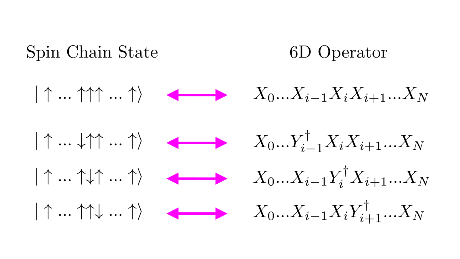
We show that this operator mixing can be phrased in terms of a spin chain with nearest neighbor hopping terms. A perturbative analysis on the tensor branch of the 6D SCFT reveals that the two-point functions for “neighboring” impurity insertions are indeed non-zero, but that in the large $N$ limit, the amount of such mixing is actually quite small. Indeed, in a diagonalized operator basis, we find that the eigenvalues for such hopping terms are of order $g^{2}/N^{2}$, where $g$ denotes a dimensionful coupling constant obtained from working on the tensor branch. One of the main observations that we will make in this paper is that a hopping term of this form will provide an indication that certain subsectors of the theory have operator mixing controlled by a 1D spin chain.

Of course, if our ultimate goal is to study operators at the conformal fixed point, we must find a way to return to strong coupling. To accomplish this, we consider the string theory background obtained from compactifying on a further circle. Retaining all of the Kaluza–Klein modes, we can treat this as a 5D “Kaluza–Klein” (5D KK theory) in which operator dimensions have their 5D values, but in which local operators are allowed to have support on all six spacetime dimensions. Using the embedding of this 5D KK theory in a string compactification, we can fix the value of the gauge coupling and evaluate the resulting hopping terms. This results in a matrix of anomalous dimensions, in accord with similar results obtained in the four-dimensional case where there are marginal coupling constants.

We perform this computation of operator mixing for a variety of 4D and 6D theories, beginning with the cases where we have the most control, i.e. where $G_{i}=SU(K)$ for all $i$. As far as we are aware, the type of operator mixing we consider has not been studied previously even in the 4D case, the closest analog being the “T-dual” computations performed in references [27, 28, 29] which also presented tantalizing hints of integrability in 4D $\mathcal{N}=2$ SCFTs. With this in place, we then consider the case of a 6D SCFT with just $SU(K)$ gauge group factors, illustrating the close similarity with the 4D case. Applying our 5D KK regulator, we show that we again get a controlled perturbative expansion inversely in the R-charge of our operators. In this case, the spin chain in question consists of spin $s=1/2$ excitations and operator mixing is controlled by the Heisenberg spin chain Hamiltonian [30]:

$$H_{A}=-\lambda_{A}\underset{i}{\sum}\left(2\overrightarrow{S}_{i}\cdot\overrightarrow{S}_{i+1}-\frac{1}{2}\right),$$

(1.6)

where the constant $\lambda_{A}$ is computable both in 4D and 6D. The spectrum of energies in this theory corresponds to the spectrum of anomalous dimensions for operators in this subsector. Importantly, this Hamiltonian defines an integrable system and as such the quasi-particle spectrum is amenable to methods such as the Bethe ansatz [31] and its modern incarnations (see e.g. [32]), and has figured prominently in the study of integrability in $\mathcal{N}=4$ super Yang–Mills theory (see e.g. [33] and reference [34] for an overview). So, we immediately gain a great deal of insight into the operator spectrum of 6D SCFTs. One can also consider generalizations of the A-type quivers in which the ranks of the gauge groups are not all constant. This leads to a broader class of spin chain Hamiltonians, and which in turn lead to modified dispersion relations for quasi-particle excitations.

Similar structure persists in the case of generalized quivers with D- and E-type gauge groups, though here, the spin excitations are associated with conformal matter operators, and so we have a more general spin chain with spin $s>1/2$ excitations. The important point for us is that the holographic duals of all these cases are rather similar, being given by the M-theory background $AdS_{7}\times S^{4}/\Gamma_{ADE}$ with $\Gamma_{ADE}$ a finite subgroup of $SU(2)$ (see e.g. [18]). This similarity provides a strong hint that the class of excitations give in (1.4) for the D- and E-series should also be controlled by an integrable spin chain. Making the well-motivated assumption that integrability persists for the D- and E-series, we also show how to extract the related spin chain Hamiltonians for all the other cases. This is in turn controlled by integrability of the $XXX_{s}$ spin chain, and the form of the Hamiltonian is then:

$$H_{G}=-\lambda_{G}\underset{i}{\sum}{Q_{2s}(\overrightarrow{S}_{i}\cdot\overrightarrow{S}_{i+1})},$$

(1.7)

where $Q_{2s}$ is a polynomial of degree $2s$ with relative coefficients fixed by the condition of integrability. In this case, our task reduces to determining the constant $\lambda_{G}$, something we carry out for all of the related 4D and 6D SCFTs.

In all these cases, the spectrum of excitations is again controlled by a spin chain with open boundary conditions. We note that the case of periodic boundary conditions is also of interest and leads to a characterization of some operators in the little string theory (LST) obtained by gauging the diagonal subgroup of $G_{0}\times G_{N+1}$ (see reference [35]). LSTs are especially intriguing because even though they are inherently non-local (at high energies), they have a low energy effective field theory with operator content closely related to their 6D SCFT counterparts.

Though we primarily focus on the operators of line (1.4), the topology of these generalized quivers also permits us to construct related spin chains. As an example, we can consider operators such as:

$$\mathcal{B}_{i}=\sqrt{\mathcal{Z}_{\mathcal{B}_{i}}}X_{0}...X_{i}(Y_{i}X_{i})X_{i+1}...X_{N},$$

(1.8)

and track the movement of the $(Y_{i}X_{i})$ insertion. We can also construct closed loops in a generalized quiver such as:

$$\mathcal{C}_{i,i+L}=\sqrt{\mathcal{Z}_{\mathcal{C}_{i,i+L}}}\mathrm{Tr}(X_{i}...X_{i+L}Y_{i+L}...Y_{i})$$

(1.9)

in the obvious notation. The level of protection from operator mixing is lower in these cases, since there are transitions to multi-trace operators. Such transitions can be suppressed if we also assume that the rank of the gauge groups in the generalized quiver are sufficiently large so that only planar diagrams contribute. Provided the R-charge (i.e. the length of the spin chain) is large enough, we again find a perturbative expansion in inverse powers of the R-charge. This leads to a quite similar analysis for impurity insertions and operator mixing, but with different boundary conditions for the associated spin chain problem.

A pleasant feature of the $\mathcal{C}$ spin chain operators is that in the large $N$ limit, perturbations can also be detected in the holographic dual theories, provided we also take $L\sim N^{1/3}$. Indeed, this leads to the pp-wave limit of the geometry $AdS_{7}\times S^{4}/\Gamma_{ADE}$, the same sort studied in [21, 36]. In the holographic dual with orbifold fixed points of $S^{4}/\Gamma_{ADE}$ at the north and south pole, the original operators of interest correspond to gravitons with large momenta orbiting along a fixed latitude, the precise location of which depends on the values of $i$ and $i+L$ in equation (1.9). Again, we note that unless we also assume that the ranks of the flavor groups scale to large size so as to remain in the planar limit, there is significant mixing with multi-trace operators.

The rest of this paper is organized as follows. We begin in section 2 by reviewing the generalized quiver picture of 6D SCFTs, and in particular present our main hypotheses and assumptions on the properties of 6D conformal matter. With this in place, we turn to some examples of quivers with A-type gauge groups, considering the case of 4D SCFTs in section 3 and 6D SCFTs in section 4. In particular, we establish the existence of a nearly-protected sector of operators with mixing controlled by a matrix of anomalous dimensions which resembles “hopping terms” in a 1D spin chain. Following this, we turn in section 5 to a further generalization of these considerations to generalized quivers with D- and E-type quivers, both for 4D and 6D SCFTs. We present our conclusions in section 6. Some additional technical details are presented in the Appendices.

In this section we briefly review some aspects of 6D SCFTs, in particular the fact that on a partial tensor branch they all resemble generalized quivers. Our aim will be to exploit this structure to extract additional details on the operator content of these fixed points. With this in mind, we first briefly review the construction of these theories, both in F-theory and M-theory. We then turn to an analysis of 6D conformal matter, and in particular the expectation that there are specific operators which can be used to build large composite operators.

Having introduced the main features of generalized quivers in 6D SCFTs, our aim will now be to understand operator mixing in some specific operator subsectors.

As a warmup exercise, and as a subject of interest in its own right, in this section we consider 4D $\mathcal{N}=2$ SCFTs with A-type gauge groups arranged along a linear quiver. We show that, much as in [21] (see also [36, 51]), there are subsectors of operators which exhibit operator mixing as controlled by a 1D spin chain, even when we pass to very large gauge coupling $g$. We accomplish this by constructing an alternative perturbative expansion in the large R-charge, $J$ of our operators. This expansion is valid in the regime where $g^{2}/J^{2}$ is small. It is important to note that the results of [21] do not carry over to the 4D $\mathcal{N}=2$ setup in general [52, 53, 54]. In our case, it is vital that the R-charge, $J$, corresponding to the length of the quiver, is large, and this adds a significant additional suppression beyond that of [21].

As far as we are aware, the specific class of operators we consider has not been previously studied, the closest analog being the analysis of [27] as well as [28] which feature a T-dual quiver gauge theory. We will comment on the relation to the T-dual setup later.

Consider then the specific 4D $\mathcal{N}=2$ quiver gauge theory:

$$[G_{0}]-G_{1}-...-G_{N}-[G_{N+1}],$$

(3.1)

where here, each gauge group factor corresponds to $G_{i}=SU(K)$. In this case, we have bifundamental hypermultiplets $X_{i}\oplus Y_{i}^{{\dagger}}$ between each link. There is a $1/2$-BPS operator of dimension $\Delta=(N+1)$ given by:^dd d This operator is in fact the superconformal primary of a short $B_{1}\overline{B}_{1}[0;0]^{(N+1,0)}$-multiplet [55] (also sometimes referred as $\widehat{\mathcal{B}}_{N+1}$ in the nomenclature of [56]).

$$\mathcal{O}_{\text{pure}}=\sqrt{\mathcal{Z}_{N}}X_{0}...X_{N},$$

(3.2)

in the obvious notation. From this starting point, we can consider inserting “impurities,” by swapping out $X$’s for $Y^{{\dagger}}$’s. For example, we can insert one such impurity, leading to the operator:

$$\mathcal{O}_{i}=\sqrt{\mathcal{Z}_{N}}\,X_{0}...X_{i-1}Y_{i}^{{\dagger}}X_{i+1}...X_{N}\,.$$

(3.3)

One can also consider adding further impurities, and provided the total number is much smaller than $N$, we remain in the dilute gas approximation and can treat the structure of correlation functions in a similar way. We first focus on the case of a single impurity insertion since the generalization to multiple impurities (at least in the dilute gas approximation) follows a similar line of analysis.

We now proceed to the evaluation of operator mixing in this setup. In our conventions, the two-point function for a free scalar will be normalized so that:

$$\left\langle(X_{i}^{{\dagger}})_{B_{i}}^{A_{i+1}}(x)(X_{i})_{B_{i+1}}^{A_{i}}(0)\right\rangle=\frac{\delta_{B_{i+1}}^{A_{i+1}}\delta_{B_{i}}^{A_{i}}}{\left|x\right|^{2\Delta_{X}}},$$

(3.4)

where $\Delta_{X}=1$ for a 4D free field. Here, the $A$ superscript and $B$ subscript indicate the components of the bifundamental representation. With this convention, applying Wick’s theorem to the two-point functions of $\mathcal{O}_{i}$ one ends up with traces over the indices of the gauge groups, each contributing a factor of $K$, so in this case the normalization factor is $\mathcal{Z}_{N}=K^{-N}$.

To begin, we observe that if we switch off the gauge couplings, the scaling dimension of each $\mathcal{O}_{i}$ is simply $\Delta_{i}=(N+1)$. Once we switch on gauge interactions, we can expect the two-point functions for the $\mathcal{O}_{i}$ to non-trivially mix. Our aim will be to determine corrections to the two-point function:

$$\left\langle\mathcal{O}_{i}^{{\dagger}}(x)O_{j}(0)\right\rangle=\frac{1}{\left|x\right|^{2\Delta_{i}}}\times\left(\delta_{ij}-\gamma_{ij}\log\left(\left|x\right|^{2}\Lambda^{2}\right)+...\right).$$

(3.5)

Here, $\gamma_{ij}$ refers to the matrix of anomalous dimensions. The main idea is that in a basis of eigenoperators for the dilatation operator, we can expect a shift in the scaling dimension, and this generates a logarithmic correction term:

$$\frac{1}{\left|x\right|^{2(\Delta+\gamma)}}=\frac{1}{\left|x\right|^{2\Delta}}\times\left(1-\gamma\log\left(\left|x\right|^{2}\Lambda^{2}\right)+...\right).$$

(3.6)

Let us now turn to operator mixing in this quiver gauge theory. We begin by working to leading order in perturbation theory in the gauge couplings $g_{i}^{2}$ but then show that the large R-charge limit allows us to form an improved perturbation series. At first order in perturbation theory, the operator mixing is controlled by the scalar potential of the $\mathcal{N}=2$ theory. To work this out, it is convenient to work in terms of the language of 4D $\mathcal{N}=1$ supersymmetry. In this case, each $X_{i}$ denotes a bifundamental chiral multiplet and each $Y_{i}$ denotes a bifundamental in the conjugate representation. Additionally, there is an adjoint-valued chiral multiplet $Z_{i}$ for each gauge group. The scalar potential is a sum of F-term and D-term contributions:

$$V=V_{F}+V_{D}.$$

(3.7)

For the D-term potential, this is just a sum over each of the gauge group nodes:

	$$\displaystyle V_{D}=\frac{1}{(4\pi^{2})^{2}}\underset{i=1}{\overset{N}{\sum}}\underset{a\in\text{adj}(G_{i})}{\sum}\frac{1}{2}D_{i,a}^{2}\,,$$		(3.8)
	$$\displaystyle D_{i,a}=g_{i}\left(\text{Tr}_{i+1}(X_{i}^{{\dagger}}T_{i,a}X_{i}-Y_{i}T_{i,a}Y_{i}^{{\dagger}})-\text{Tr}_{i-1}(X_{i-1}T_{i,a}X_{i-1}^{{\dagger}}-Y_{i-1}^{{\dagger}}T_{i,a}Y_{i-1})\right)+\cdots\,,$$		(3.9)

where we have dropped contributions from the $Z_{i}$ scalars since they do not contribute at leading order to operator mixing. The overall normalization by $1/(4\pi^{2})^{2}$ is due to our normalization of the $X^{{\dagger}}X$ two-point function.^ee e With canonically normalized kinetic terms for free fields, we would instead have a two point function $$\left\langle(X_{i}^{{\dagger}})_{B_{i}}^{A_{i+1}}(x)(X_{i})_{B_{i+1}}^{A_{i}}(0)\right\rangle=\frac{1}{4\pi^{2}}\frac{\delta_{B_{i+1}}^{A_{i+1}}\delta_{B_{i}}^{A_{i}}}{\left|x\right|^{2\Delta_{X}}},$$ (3.10) with $\Delta_{X}=1$ for a 4D free field. Here, the $T_{i,a}$ are Lie algebra generators for $G_{i}$, Tr_i+1 and Tr_i-1 indicate a further instruction to sum over all of the indices of adjacent nodes in the quiver. We also have the F-term potential contributions from the chiral multiplet $Z_{i}$, which we denote as $F_{i,a}$:

$$V_{F}=\frac{1}{(4\pi^{2})^{2}}\underset{i=1}{\overset{N}{\sum}}\underset{a\in\text{adj}(G_{i})}{\sum}\left|F_{i,a}\right|^{2}+\cdots\,,$$

(3.11)

where the “$...$” refers to contributions from the other chiral multiplets, which again do not influence operator mixing at leading order. Here, we have:

$$F_{i,a}=\sqrt{2}g_{i}\left(\text{Tr}_{i+1}(Y_{i}T_{i,a}X_{i})-\text{Tr}_{i-1}(X_{i-1}T_{i,a}Y_{i-1})\right).$$

(3.12)

From this, we can deduce that operator mixing is indeed possible. Since our scalar potential only contains interaction terms between hypermultiplets on neighboring links, we see that to leading order in perturbation theory the operator $\mathcal{O}_{i}$, can only have a non-trivial two-point function with $\mathcal{O}_{i-1}$, $\mathcal{O}_{i+1}$ and $\mathcal{O}_{i}$.

The computation of the “hopping terms” involves only a contribution from the F-term potential, see figure 4. In the case of hopping between $\mathcal{O}_{i}$ and $\mathcal{O}_{i-1}$, the relevant contribution comes from $\left|F_{i,a}\right|^{2}$. We find the leading order contribution (evaluated in Euclidean signature):

$$\left<\mathcal{O}_{i}^{{\dagger}}(x)\mathcal{O}_{i-1}(0)\right>=\frac{1}{\left|x\right|^{2\Delta_{0}}}\times\left(1+\frac{2g_{i}^{2}\widetilde{C}_{i}}{(4\pi^{2})^{2}}\int d^{4}z\frac{\left|x\right|^{4\Delta_{X}}}{\left|x-z\right|^{4\Delta_{X}}}\frac{1}{\left|z\right|^{4\Delta_{X}}}+\dots\right)\,,$$

(3.13)

where we have suppressed flavor index structure. Here, $\Delta_{0}$ refers to the scaling dimension with all gauge couplings switched off and $\widetilde{C}_{i+1}$ is a combinatorial factor obtained from the quadratic Casimir of the fundamental representation and its dimension, given by evaluating:

$$\widetilde{C}_{i}=\frac{1}{d_{F}}\underset{a\in\text{adj}(G_{i})}{\sum}\text{Tr}_{\text{fund}}(T_{i,a}T_{i,a})=\frac{f_{G_{i}}}{h_{G_{i}}^{\vee}d_{F}}\times\dim G_{i}\,,$$

(3.14)

where $d_{F}$ is the dimension of the fundamental representation of $G_{i}$, and with $h_{G}^{\vee}$ the dual Coxeter number of the group $G$. The righthand side of (3.14) is obtained from evaluating traces in different representations. To fix our normalizations we use the same notation as in [57], and introduce an auxiliary field strength $F$ to relate the various traces in different representations as follows:

$$\mathrm{Tr}_{\mathrm{fund}}F^{2}=f_{G}\mathrm{Tr}F^{2}\,,\qquad\mathrm{Tr}_{\mathrm{adj}}F^{2}=h_{G}^{\vee}\mathrm{Tr}F^{2}\,.$$

(3.15)

For a quiver with all $SU(K)$ factors, we have $f_{G}=1/2$ and $h_{G}^{\vee}=K$. In Appendix B we evaluate the loop integral appearing in (3.13). Setting $\Delta_{X}=1$, there is indeed a logarithmic contribution, and we wind up with:

$$\left\langle\mathcal{O}_{i}^{{\dagger}}(x)\mathcal{O}_{i-1}(0)\right\rangle=\frac{1}{\left|x\right|^{2\Delta_{0}}}\left(1+\frac{g_{i}^{2}\widetilde{C}_{i}}{8\pi^{2}}\times\log(\left|x\right|^{2}\Lambda^{2})+...\right).$$

(3.16)

Closely related to this case is the two-point function $\left\langle\mathcal{O}_{i}^{{\dagger}}(x)\mathcal{O}_{i+1}(0)\right\rangle$. The only contribution comes from $\left|F_{i+1,a}\right|^{2}$. The computation is otherwise the same, so we get:

$$\left\langle\mathcal{O}_{i}^{{\dagger}}(x)\mathcal{O}_{i+1}(0)\right\rangle=\frac{1}{\left|x\right|^{2\Delta_{0}}}\times\left(1+\frac{g_{i+1}^{2}\widetilde{C}_{i+1}}{8\pi^{2}}\times\log(\left|x\right|^{2}\Lambda^{2})+...\right).$$

(3.17)

Finally, we have the “stationary term” associated with the evaluation of $\left\langle\mathcal{O}_{i}^{{\dagger}}(x)\mathcal{O}_{i}(0)\right\rangle$. This case is clearly somewhat more subtle because there are far more contributions, which include contributions both from the scalar potential, as well as t-channel vector boson exchange. On general grounds, we expect there to be a zero mode in the anomalous dimension matrix since we know that one linear combination of the $\mathcal{O}_{i}$ is in the same $SU(2)_{\mathcal{R}}$ R-symmetry multiplet as $\mathcal{O}_{\mathrm{pure}}$. Jumping ahead to equation (3.21), we will indeed find that this is the case, provided we fix the relative strengths of the matrix entries.

In stringy terms we can argue as follows: starting from $K$ D3-branes probing $\mathbb{C}\times\mathbb{C}^{2}$, we can consider the related correlation functions obtained from working in terms of the D3-brane probe of $\mathbb{C}\times\mathbb{C}^{2}/\mathbb{Z}_{N+1}$. Doing so, we generate a circular quiver with $N+1$ gauge group nodes $G_{i}=SU(K)$. We can arrive at this sort of quiver by gauging a diagonal subgroup of $G_{0}\times G_{N+1}$. The evaluation of BMN-like operators is thus quite close to our computation, and for the same reasons as presented there, we conclude that the relevant contribution to the hopping term is essentially the same, at least when all gauge couplings are equal. In that setting, the contribution to the diagonal is a factor of $-2$ relative to the off-diagonal hopping terms.

Another way to argue for this is to observe that if we include all contributions other than those from the F-term contributions, we expect an exact cancellation, much as in the computations of reference [28]. That leaves us to include the contributions from $\left|F_{i,a}\right|^{2}$ and $\left|F_{i+1,a}\right|^{2}$. This leads us to our formula:

$$\left\langle\mathcal{O}_{i}^{{\dagger}}(x)\mathcal{O}_{i}(0)\right\rangle=\frac{1}{\left|x\right|^{2\Delta_{0}}}\times\left(1-\frac{1}{8\pi^{2}}\left(g_{i}^{2}\widetilde{C}_{i}+g_{i+1}^{2}\widetilde{C}_{i+1}\right)\log(\left|x\right|^{2}\Lambda^{2})+...\right).$$

(3.18)

Summarizing, we have extracted the anomalous dimension matrix with non-zero entries:

	$\displaystyle\gamma_{ii}$	$\displaystyle=\frac{1}{8\pi^{2}}\left(g_{i}^{2}\widetilde{C}_{i}+g_{i+1}^{2}\widetilde{C}_{i+1}\right)$		(3.19)
	$\displaystyle\gamma_{i,i+1}$	$\displaystyle=\gamma_{i+1,i}=-\frac{g_{i+1}^{2}\widetilde{C}_{i+1}}{8\pi^{2}},$		(3.20)

for $i=0,...,N$. Setting $g_{i}^{2}=g^{2}$ for $i=1,...,N$ and $g_{0}^{2}=g_{N+1}^{2}=0$, we can also write this as a 1D Lattice Laplacian with non-trivial boundary conditions:

$$\underline{\gamma}=\lambda_{G}\left[\begin{array}[c]{ccccc}1&-1&&&\\ -1&2&-1&&\\ &-1&...&-1&\\ &&-1&2&-1\\ &&&-1&1\end{array}\right],$$

(3.21)

where $\lambda_{G}$ is the overall normalization for the Hamiltonian and is given by:

$$\lambda_{G}=\frac{g^{2}\widetilde{C}_{G}}{8\pi^{2}},$$

(3.22)

for a general gauge group $G$, with $\widetilde{C}_{G}$ as in equation (3.14) evaluated in the special case $G=SU(K)$. Note that equation (3.21) is in accord with having a zero mode.

It is also instructive to extract the linear combination of $\mathcal{O}_{i}$ which are diagonal under the action of the anomalous dimension matrix. We find operators $\widetilde{\mathcal{O}}_{p}$ with scaling dimensions:

	$\displaystyle\widetilde{\mathcal{O}}_{p}$	$\displaystyle=\frac{1}{\sqrt{N+1}}\underset{j=0}{\overset{N}{\sum}}\cos\left(p\left(j+\frac{1}{2}\right)\right)\mathcal{O}_{j}$		(3.23)
	$\displaystyle(\Delta-\Delta_{0})_{p}$	$\displaystyle=4\lambda_{G}\sin^{2}\left(\frac{p}{2}\right)\text{ \ \ with \ }\lambda_{G}=\frac{g^{2}}{8\pi^{2}}\frac{f_{G}\dim G}{h_{G}^{\vee}d_{F}}$		(3.24)

where the original dimension is $\Delta_{0}=(N+1)$ and the eigenoperator, $\widetilde{O}_{p}$, is interpreted as a magnon with quantized momentum, $p=\frac{\pi m}{N+1}\,,m=0,1,\dots,N$. These $\widetilde{O}_{p}$ are the eigenoperators for the operator mixing captured by the one-loop two-point function given in (3.18). The important point for us is that just as in [21], even though we performed a perturbative expansion in $g^{2}$, we can expand at large $N$. In this limit, we observe that even if $g^{2}$ becomes large, we can continue to work to leading order in perturbation theory provided $g^{2}/N^{2}$ remains small.

References

- [1] E. Witten, “Some comments on string dynamics,” in STRINGS 95: Future Perspectives in String Theory, pp. 501–523. 7, 1995. arXiv:hep-th/9507121.
- [2] A. Strominger, “Open p-branes,” Phys. Lett. B 383 (1996) 44–47, arXiv:hep-th/9512059.
- [3] N. Seiberg, “Nontrivial fixed points of the renormalization group in six-dimensions,” Phys. Lett. B 390 (1997) 169–171, arXiv:hep-th/9609161.
- [4] C. Vafa, “Geometric origin of Montonen-Olive duality,” Adv. Theor. Math. Phys. 1 (1998) 158–166, arXiv:hep-th/9707131.
- [5] E. Witten, “Solutions of four-dimensional field theories via M theory,” Nucl. Phys. B 500 (1997) 3–42, arXiv:hep-th/9703166.
- [6] D. Gaiotto, “ Dualities,” JHEP 08 (2012) 034, arXiv:0904.2715 [hep-th].
- [7] S. S. Razamat and G. Zafrir, “ Conformal Dualities,” JHEP 09 (2019) 046, arXiv:1906.05088 [hep-th].
- [8] J. J. Heckman, D. R. Morrison, and C. Vafa, “On the Classification of 6D SCFTs and Generalized ADE Orbifolds,” JHEP 05 (2014) 028, arXiv:1312.5746 [hep-th]. [Erratum: JHEP 06, 017 (2015)].
- [9] J. J. Heckman, D. R. Morrison, T. Rudelius, and C. Vafa, “Atomic Classification of 6D SCFTs,” Fortsch. Phys. 63 (2015) 468–530, arXiv:1502.05405 [hep-th].
- [10] L. Bhardwaj, “Classification of 6d gauge theories,” JHEP 11 (2015) 002, arXiv:1502.06594 [hep-th].
- [11] L. Bhardwaj, “Revisiting the classifications of 6d SCFTs and LSTs,” JHEP 03 (2020) 171, arXiv:1903.10503 [hep-th].
- [12] J. J. Heckman and T. Rudelius, “Top Down Approach to 6D SCFTs,” J. Phys. A 52 no. 9, (2019) 093001, arXiv:1805.06467 [hep-th].
- [13] C. Beem, M. Lemos, L. Rastelli, and B. C. van Rees, “The (2, 0) superconformal bootstrap,” Phys. Rev. D 93 no. 2, (2016) 025016, arXiv:1507.05637 [hep-th].
- [14] C.-M. Chang and Y.-H. Lin, “Carving Out the End of the World or (Superconformal Bootstrap in Six Dimensions),” JHEP 08 (2017) 128, arXiv:1705.05392 [hep-th].
- [15] L. F. Alday and X. Zhou, “All Tree-Level Correlators for M-theory on ,” arXiv:2006.06653 [hep-th].
- [16] F. Apruzzi, M. Fazzi, D. Rosa, and A. Tomasiello, “All AdS7 Solutions of type II supergravity,” JHEP 04 (2014) 064, arXiv:1309.2949 [hep-th].
- [17] D. Gaiotto and A. Tomasiello, “Holography for (1,0) theories in six dimensions,” JHEP 12 (2014) 003, arXiv:1404.0711 [hep-th].
- [18] M. Del Zotto, J. J. Heckman, A. Tomasiello, and C. Vafa, “6d Conformal Matter,” JHEP 02 (2015) 054, arXiv:1407.6359 [hep-th].
- [19] K. Filippas, C. Núñez, and J. Van Gorsel, “Integrability and holographic aspects of six-dimensional superconformal field theories,” JHEP 06 (2019) 069, arXiv:1901.08598 [hep-th].
- [20] O. Bergman, M. Fazzi, D. Rodríguez-Gómez, and A. Tomasiello, “Charges and holography in 6d (1,0) theories,” JHEP 05 (2020) 138, arXiv:2002.04036 [hep-th].
- [21] D. E. Berenstein, J. M. Maldacena, and H. S. Nastase, “Strings in flat space and pp waves from N=4 superYang-Mills,” JHEP 04 (2002) 013, arXiv:hep-th/0202021.
- [22] S. Hellerman, D. Orlando, S. Reffert, and M. Watanabe, “On the CFT Operator Spectrum at Large Global Charge,” JHEP 12 (2015) 071, arXiv:1505.01537 [hep-th].
- [23] J. J. Heckman, “More on the Matter of 6D SCFTs,” Phys. Lett. B 747 (2015) 73–75, arXiv:1408.0006 [hep-th].
- [24] J. J. Heckman, T. Rudelius, and A. Tomasiello, “6D RG Flows and Nilpotent Hierarchies,” JHEP 07 (2016) 082, arXiv:1601.04078 [hep-th].
- [25] J. J. Heckman, T. Rudelius, and A. Tomasiello, “Fission, Fusion, and 6D RG Flows,” JHEP 02 (2019) 167, arXiv:1807.10274 [hep-th].
- [26] F. Hassler, J. J. Heckman, T. B. Rochais, T. Rudelius, and H. Y. Zhang, “T-Branes, String Junctions, and 6D SCFTs,” Phys. Rev. D 101 no. 8, (2020) 086018, arXiv:1907.11230 [hep-th].
- [27] N. Beisert and R. Roiban, “The Bethe ansatz for orbifolds of super Yang-Mills theory,” JHEP 11 (2005) 037, arXiv:hep-th/0510209.
- [28] A. Gadde, E. Pomoni, and L. Rastelli, “Spin Chains in N=2 Superconformal Theories: From the Z_2 Quiver to Superconformal QCD,” JHEP 06 (2012) 107, arXiv:1006.0015 [hep-th].
- [29] E. Pomoni, “4D SCFTs and spin chains,” arXiv:1912.00870 [hep-th].
- [30] W. Heisenberg, “Zur Theorie des Ferromagnetismus,” Z. Phys. 49 no. 9-10, (1928) 619–636.
- [31] H. Bethe, “Zur Theorie der Metalle. I. Eigenwerte und Eigenfunktionen der linearen Atomkette,” Z. Phys. 71 (1931) 205–226.
- [32] L. Faddeev, “How algebraic Bethe ansatz works for integrable model,” in Les Houches School of Physics: Astrophysical Sources of Gravitational Radiation, pp. pp. 149–219. 5, 1996. arXiv:hep-th/9605187.
- [33] J. Minahan and K. Zarembo, “The Bethe Ansatz for Super Yang-Mills,” JHEP 03 (2003) 013, arXiv:hep-th/0212208.
- [34] N. Beisert et al., “Review of AdS/CFT Integrability: An Overview,” Lett. Math. Phys. 99 (2012) 3–32, arXiv:1012.3982 [hep-th].
- [35] L. Bhardwaj, M. Del Zotto, J. J. Heckman, D. R. Morrison, T. Rudelius, and C. Vafa, “F-theory and the Classification of Little Strings,” Phys. Rev. D 93 no. 8, (2016) 086002, arXiv:1511.05565 [hep-th]. [Erratum: Phys.Rev.D 100, 029901 (2019)].
- [36] D. E. Berenstein, E. Gava, J. M. Maldacena, K. S. Narain, and H. S. Nastase, “Open strings on plane waves and their Yang-Mills duals,” arXiv:hep-th/0203249.
- [37] E. Witten, “Toroidal compactification without vector structure,” JHEP 02 (1998) 006, arXiv:hep-th/9712028.
- [38] Y. Tachikawa, “Frozen singularities in M and F theory,” JHEP 06 (2016) 128, arXiv:1508.06679 [hep-th].
- [39] L. Bhardwaj, D. R. Morrison, Y. Tachikawa, and A. Tomasiello, “The frozen phase of F-theory,” JHEP 08 (2018) 138, arXiv:1805.09070 [hep-th].
- [40] J. J. Heckman and L. Tizzano, “6D Fractional Quantum Hall Effect,” JHEP 05 (2018) 120, arXiv:1708.02250 [hep-th].
- [41] M. Bershadsky and A. Johansen, “Colliding Singularities in F-theory and Phase Transitions,” Nucl. Phys. B 489 (1997) 122–138, arXiv:hep-th/9610111.
- [42] P. S. Aspinwall and D. R. Morrison, “Point-like Instantons on K3 Orbifolds,” Nucl. Phys. B 503 (1997) 533–564, arXiv:hep-th/9705104.
- [43] D. R. Morrison and W. Taylor, “Classifying Bases for 6D F-theory Models,” Central Eur. J. Phys. 10 (2012) 1072–1088, arXiv:1201.1943 [hep-th].
- [44] K. Ohmori, H. Shimizu, Y. Tachikawa, and K. Yonekura, “6d theories on and class S theories: Part I,” JHEP 07 (2015) 014, arXiv:1503.06217 [hep-th].
- [45] K. Ohmori, H. Shimizu, Y. Tachikawa, and K. Yonekura, “6d theories on S1 /T2 and class S theories: part II,” JHEP 12 (2015) 131, arXiv:1508.00915 [hep-th].
- [46] F. Apruzzi, J. J. Heckman, D. R. Morrison, and L. Tizzano, “4D Gauge Theories with Conformal Matter,” JHEP 09 (2018) 088, arXiv:1803.00582 [hep-th].
- [47] A. Bourget, S. Cabrera, J. F. Grimminger, A. Hanany, M. Sperling, A. Zajac, and Z. Zhong, “The Higgs mechanism — Hasse diagrams for symplectic singularities,” JHEP 01 (2020) 157, arXiv:1908.04245 [hep-th].
- [48] N. Seiberg, “Five-dimensional SUSY field theories, nontrivial fixed points and string dynamics,” Phys. Lett. B 388 (1996) 753–760, arXiv:hep-th/9608111.
- [49] M. R. Douglas, S. H. Katz, and C. Vafa, “Small instantons, Del Pezzo surfaces and type I-prime theory,” Nucl. Phys. B 497 (1997) 155–172, arXiv:hep-th/9609071.
- [50] D. R. Morrison and N. Seiberg, “Extremal transitions and five-dimensional supersymmetric field theories,” Nucl. Phys. B 483 (1997) 229–247, arXiv:hep-th/9609070.
- [51] D. Berenstein and S. E. Vazquez, “Integrable open spin chains from giant gravitons,” JHEP 06 (2005) 059, arXiv:hep-th/0501078.
- [52] T. Nishioka and T. Takayanagi, “On Type IIA Penrose Limit and N=6 Chern-Simons Theories,” JHEP 08 (2008) 001, arXiv:0806.3391 [hep-th].
- [53] N. Gromov and G. Sizov, “Exact Slope and Interpolating Functions in N=6 Supersymmetric Chern-Simons Theory,” Phys. Rev. Lett. 113 no. 12, (2014) 121601, arXiv:1403.1894 [hep-th].
- [54] V. Mitev and E. Pomoni, “Exact Bremsstrahlung and Effective Couplings,” JHEP 06 (2016) 078, arXiv:1511.02217 [hep-th].
- [55] C. Cordova, T. T. Dumitrescu, and K. Intriligator, “Multiplets of Superconformal Symmetry in Diverse Dimensions,” arXiv:1612.00809 [hep-th].
- [56] F. A. Dolan and H. Osborn, “On short and semi-short representations for four-dimensional superconformal symmetry,” Annals Phys. 307 (2003) 41–89, arXiv:hep-th/0209056.
- [57] K. Ohmori, H. Shimizu, Y. Tachikawa, and K. Yonekura, “Anomaly Polynomial of General 6d SCFTs,” PTEP 2014 no. 10, (2014) 103B07, arXiv:1408.5572 [hep-th].
- [58] Y. Wang, W.-L. Yang, J. Cao, and K. Shi, Off-Diagonal Bethe Ansatz for Exactly Solvable Models. Springer-Verlag, 2015.
- [59] O. Aharony, S. S. Gubser, J. M. Maldacena, H. Ooguri, and Y. Oz, “Large N field theories, string theory and gravity,” Phys. Rept. 323 (2000) 183–386, arXiv:hep-th/9905111.
- [60] M. R. Douglas and G. W. Moore, “D-branes, quivers, and ALE instantons,” arXiv:hep-th/9603167.
- [61] J. D. Blum and K. A. Intriligator, “New phases of string theory and 6-D RG fixed points via branes at orbifold singularities,” Nucl. Phys. B 506 (1997) 199–222, arXiv:hep-th/9705044.
- [62] J. Polchinski, String theory. Vol. 2: Superstring theory and beyond. Cambridge Monographs on Mathematical Physics. Cambridge University Press, 12, 2007.
- [63] J. M. Maldacena, “The Large N limit of superconformal field theories and supergravity,” Int. J. Theor. Phys. 38 (1999) 1113–1133, arXiv:hep-th/9711200.
- [64] E. Witten, “Baryons and branes in anti-de Sitter space,” JHEP 07 (1998) 006, arXiv:hep-th/9805112.
- [65] V. Balasubramanian, M. Berkooz, A. Naqvi, and M. J. Strassler, “Giant gravitons in conformal field theory,” JHEP 04 (2002) 034, arXiv:hep-th/0107119.
- [66] M. Buican, J. Hayling, and C. Papageorgakis, “Aspects of Superconformal Multiplets in ,” JHEP 11 (2016) 091, arXiv:1606.00810 [hep-th].
- [67] H. Babujian, “Exact solution of the one-dimensional isotropic Heisenberg chain with arbitrary spin S,” Phys. Lett. A 90 (1982) 479–482.
- [68] A. Zamolodchikov and V. Fateev, “MODEL FACTORIZED S MATRIX AND AN INTEGRABLE HEISENBERG CHAIN WITH SPIN 1. (IN RUSSIAN),” Sov. J. Nucl. Phys. 32 (1980) 298–303.
- [69] P. Kulish, N. Reshetikhin, and E. Sklyanin, “Yang-Baxter Equation and Representation Theory. 1.,” Lett. Math. Phys. 5 (1981) 393–403.
- [70] P. Kulish and E. Sklyanin, “QUANTUM SPECTRAL TRANSFORM METHOD. RECENT DEVELOPMENTS,” Lect. Notes Phys. 151 (1982) 61–119.
- [71] L. Takhtajan, “The picture of low-lying excitations in the isotropic Heisenberg chain of arbitrary spins,” Phys. Lett. A 87 (1982) 479–482.
- [72] H. M. Babujian, “EXACT SOLUTION OF THE ISOTROPIC HEISENBERG CHAIN WITH ARBITRARY SPINS: THERMODYNAMICS OF THE MODEL,” Nucl. Phys. B 215 (1983) 317–336.
- [73] V. Tarasov, L. Takhtajan, and L. Faddeev, “Local Hamiltonians for integrable quantum models on a lattice,” Theor. Math. Phys. 57 (1983) 1059–1073.
- [74] V. Korepin, “Universality of Entropy Scaling in One Dimensional Gapless Models,” Phys. Rev. Lett. 92 (2004) 096402, arXiv:cond-mat/0311056.
- [75] N. Beisert and M. Staudacher, “The SYM Integrable Super Spin Chain,” Nucl. Phys. B 670 (2003) 439–463, arXiv:hep-th/0307042.
- [76] M. Martins and P. Ramos, “The Algebraic Bethe ansatz for rational braid - monoid lattice models,” Nucl. Phys. B 500 (1997) 579–620, arXiv:hep-th/9703023.
- [77] D. Arnaudon, J. Avan, N. Crampe, A. Doikou, L. Frappat, and E. Ragoucy, “Bethe ansatz equations and exact S matrices for the open super spin chain,” Nucl. Phys. B 687 (2004) 257–278, arXiv:math-ph/0310042.
- [78] K. Costello, “Integrable lattice models from four-dimensional field theories,” Proc. Symp. Pure Math. 88 (2014) 3–24, arXiv:1308.0370 [hep-th].
- [79] K. Costello, “Supersymmetric gauge theory and the Yangian,” arXiv:1303.2632 [hep-th].
- [80] K. Costello, E. Witten, and M. Yamazaki, “Gauge Theory and Integrability, I,” arXiv:1709.09993 [hep-th].
- [81] K. Costello, E. Witten, and M. Yamazaki, “Gauge Theory and Integrability, II,” arXiv:1802.01579 [hep-th].