跳到论文正文
W Papers独立论文阅读器 arXiv:2007.07161 论文正文 计算阅读时间 · 0%
引用这篇论文根据当前论文元数据生成,正式投稿前建议核对。


License: arXiv.org perpetual non-exclusive license
arXiv:2007.07161v2 [cs.DS] 21 Feb 2021

Graph Sparsification
by Universal Greedy Algorithms

Ming-Jun Lai Address: Department of Mathematics, University of Georgia, Athens, GA 30602. U.S.A. Email address: mjlai@uga.edu , Jiaxin Xie Address: School of Mathematical Sciences, Beihang University, Beijing, 100191, China Email address: xiejx@buaa.edu.cn and Zhiqiang Xu Address: LSEC, Inst. Comp. Math., Academy of Mathematics and System Science, Chinese Academy of Sciences, Beijing, 100091, China
School of Mathematical Sciences, University of Chinese Academy of Sciences, Beijing 100049, China
Email address: xuzq@lsec.cc.ac.cn
Abstract.

Graph sparsification is to approximate an arbitrary graph by a sparse graph and is useful in many applications, such as simplification of social networks, least squares problems, numerical solution of symmetric positive definite linear systems and etc. In this paper, inspired by the well-known sparse signal recovery algorithm called orthogonal matching pursuit (OMP), we introduce a deterministic, greedy edge selection algorithm called universal greedy approach (UGA) for graph sparsification. For a general spectral sparsification problem, e.g., positive subset selection problem from a set of mm vectors from ℝn\mathbb{R}^{n}, we propose a nonnegative UGA algorithm which needs O⁡(m​n2+n3/ϵ2)O(mn^{2}+n^{3}/\epsilon^{2}) time to find a 1+ϵ/β1−ϵ/β\frac{1+\epsilon/\beta}{1-\epsilon/\beta}-spectral sparsifier with positive coefficients with sparsity ≤⌈nϵ2⌉\leq\lceil\frac{n}{\epsilon^{2}}\rceil, where β\beta is the ratio between the smallest length and largest length of the vectors. The convergence of the nonnegative UGA algorithm will be established. For the graph sparsification problem, another UGA algorithm will be proposed which can output a 1+O⁡(ϵ)1−O⁡(ϵ)\frac{1+O(\epsilon)}{1-O(\epsilon)}-spectral sparsifier with ⌈nϵ2⌉\lceil\frac{n}{\epsilon^{2}}\rceil edges in O⁡(m+n2/ϵ2)O(m+n^{2}/\epsilon^{2}) time from a graph with mm edges and nn vertices under some mild assumptions. This is a linear time algorithm in terms of the number of edges that the community of graph sparsification is looking for. The best result in the literature to the knowledge of the authors is the existence of a deterministic algorithm which is almost linear, i.e. O⁡(m1+o⁡(1))O(m^{1+o(1)}) for some o⁡(1)=O⁡((log⁡log⁡(m))2/3log1/3⁡(m))o(1)=O(\frac{(\log\log(m))^{2/3}}{\log^{1/3}(m)}). Finally, extensive experimental results, including applications to graph clustering and least squares regression, show the effectiveness of proposed approaches.

1. Introduction

Graph sparsification aims to find a sparse subgraph from a dense graph GG with nn vertices and mm edges (typically m≫nm\gg n) so that the sparsified subgraph can serve as a proxy for GG in numerical computations for graph-based applications. In [4], Batson, Spielman and Srivastava showed that for any undirected graph GG one can find a sparse graph (sparsifier) whose graph Laplacian matrix can well preserve the spectrum of the original graph Laplacian matrix. Such a spectral graph sparsification plays increasingly important roles in many applications areas in mathematics and computer science [23, 28, 36]. A related research, known as Laplacian Paradigm, is illustrated as an emerging paradigm for the design of scalable algorithms in recent years. We refer the reader to [33, 37, 40] for excellent surveys on its background and applications.

Mathematically, we can state the graph sparsification problem as follows. Consider a undirected and weighted graph G=(V,E,𝐰)G=(V,E,{\bf w}), where VV is a set of vertices, EE is a set of edges, and 𝐰{\bf w} is a weight function that assigns a positive weight to each edge. The Laplacian matrix of graph GG is defined by

LG=∑(u,v)∈Ew(u,v)​(𝐞u−𝐞v)​(𝐞u−𝐞v)⊤,L_{G}=\sum\limits_{(u,v)\in E}w_{(u,v)}({\bf e}_{u}-{\bf e}_{v})({\bf e}_{u}-{\bf e}_{v})^{\top},

where w(u,v)≥0w_{(u,v)}\geq 0 is the weight of edge (u,v)(u,v) and 𝐞u∈ℝ|V|{\bf e}_{u}\in\mathbb{R}^{|V|} is the characteristic vector of vertex uu (with a 11 on coordinated uu and zeros elsewhere). In other words, for any 𝐱∈ℝn{\bf x}\in\mathbb{R}^{n},

𝐱⊤​LG​𝐱=∑(u,v)∈Ew(u,v)​(𝐱⁡(u)−𝐱⁡(v))2≥0.{\bf x}^{\top}L_{G}{\bf x}=\sum\limits_{(u,v)\in E}w_{(u,v)}\big({\bf x}(u)-{\bf x}(v)\big)^{2}\geq 0.

That is, LGL_{G} is positive semidefinite. Spectral graph sparsification is the process of approximating the graph GG by a sparse (linear-sized) graph H=(V,E~,𝐰~)H=(V,\tilde{E},\tilde{\bf w}) such that

(1) a​𝐱⊤​LG​𝐱≤𝐱⊤​LH​𝐱≤b​𝐱⊤​LG​𝐱a{\bf x}^{\top}L_{G}{\bf x}\leq{\bf x}^{\top}L_{H}{\bf x}\leq b{\bf x}^{\top}L_{G}{\bf x}

for all 𝐱∈ℝ|V|{\bf x}\in\mathbb{R}^{|V|}, where b≥a>0b\geq a>0. Setting κ:=b/a\kappa:=b/a, HH is called a κ\kappa-approximation of GG or a κ\kappa-sparsifier of GG. Actually, if we restrict the inequality in (1) only for all 𝐱∈{0,1}|V|{\bf x}\in\{0,1\}^{|V|}, one can obtain the cut sparsification [6]. Batson, Spielman and Srivastava [4, Theorem 1.11.1] proved that for every weighted graph GG and every ϵ∈(0,1)\epsilon\in(0,1) there exists a weighted graph HH with at most ⌈(n−1)/ϵ2⌉\lceil(n-1)/\epsilon^{2}\rceil edges which is an (1+ϵ)2(1−ϵ)2\frac{(1+\epsilon)^{2}}{(1-\epsilon)^{2}}-approximation of LGL_{G}. More generally, let V={𝐯1,…,𝐯m}⊂ℝnV=\{{\bf v}_{1},\ldots,{\bf v}_{m}\}\subset\mathbb{R}^{n} be a collection of vectors with m≫nm\gg n. We replace LGL_{G} by

(2) B=∑i=1m𝐯i​𝐯i⊤,B=\sum_{i=1}^{m}{\bf v}_{i}{\bf v}_{i}^{\top},

which is clearly positive semidefinite. In [4, Theorem 1.21.2], the authors proved that for any ϵ∈(0,1)\epsilon\in(0,1), these exists a 𝐬=(s1,…,sm)∈ℝ+m{\bf s}=(s_{1},\ldots,s_{m})\in\mathbb{R}^{m}_{+} with ‖𝐬‖0≤⌈rank​(B)/ϵ2⌉\|{\bf s}\|_{0}\leq\lceil\mbox{rank}(B)/\epsilon^{2}\rceil such that

(3) (1−ϵ)2​B⪯∑i=1msi​𝐯i​𝐯i⊤⪯(1+ϵ)2​B,(1-\epsilon)^{2}B\preceq\sum_{i=1}^{m}s_{i}{\bf v}_{i}{\bf v}_{i}^{\top}\preceq(1+\epsilon)^{2}B,

where ℝ+m\mathbb{R}_{+}^{m} denotes the nonnegative orthant in ℝm\mathbb{R}^{m} and ‖𝐬‖0\|{\bf s}\|_{0} stands for the number of nonzero entries of vector 𝐬{\bf s}.

Our aim is to use the ideas of the well-known orthogonal matching pursuit (OMP) to study spectral sparsification problems. We first focus on the following problem:

(4) min𝐬∈ℝm,𝐬≥0⁡‖𝐬‖0s.t.(1−ϵ)2​B⪯∑i=1msi​𝐯i​𝐯i⊤⪯(1+ϵ)2​B,\min_{{\bf s}\in\mathbb{R}^{m},{\bf s}\geq 0}\|{\bf s}\|_{0}\quad\text{\rm s.t.}\quad(1-\epsilon)^{2}B\preceq\sum_{i=1}^{m}s_{i}{\bf v}_{i}{\bf v}_{i}^{\top}\preceq(1+\epsilon)^{2}B,

where B=∑i=1m𝐯i​𝐯i⊤B=\sum_{i=1}^{m}{\bf v}_{i}{\bf v}_{i}^{\top} and {𝐯1​…,𝐯m}⊂ℝn\{{\bf v}_{1}\ldots,{\bf v}_{m}\}\subset\mathbb{R}^{n}.

We shall call (4) sparse positive subset selection problem and will study it first. For convenience, we shall start with the isotropic case, i.e., when B=InB=I_{n} is the n×nn\times n identity matrix. Such decomposition appear in many areas of mathematics and are also called isotropic sets, tight frames, John’s decompositions (when their mean is zero), etc. We shall also explain how to do with general symmetric positive semidefinite matrix BB. Mainly we shall provide an algorithm called nonnegative UGA algorithm to find such a sparse subset with positive coefficients and establish the convergence of the algorithm. Then we solve graph sparsification problem using a similar UGA algorithm and establish the convergence.

1.1. Related work

In recent years, spectral sparsification is a widely studied topic and has applications to many areas in mathematics and theoretical computer science. Recent work includes [2, 3, 4, 5, 8, 10, 15, 16, 19, 21, 22, 23, 24, 26, 27, 32, 34, 35, 36, 44, 47, 48].

In the seminal paper [35], Spielman and Teng first introduced the notion of spectral sparsification and showed that any undirected graph GG of nn vertices and mm edges has a spectral sparsifier with O⁡(n​logc​n)O(n\log^{c}n) edges that can be computed in O⁡(m​logc​(m))O(m\log^{c}(m)) time for some positive constant cc. In terms of the number of vertices nn with assumption of the number of edges mm being O⁡(n2)O(n^{2}), the Spielman and Teng’s algorithm need O⁡(n2​2c​log2⁡(n))O(n^{2}2^{c}\log^{2}(n)) time. Some progresses had been made by the work of Spielman and Srivastava [34] and Lee and Sun [26], who showed how to find the spectral sparsifiers with O⁡(n​log⁡n)O(n\log n) and O⁡(n)O(n) edges, respectively, in O⁡(m​logc​(m))O(m\log^{c}(m)) time. We remark that all of this type of algorithms requires random sampling or random projection.

A celebrated result of Batson, Spielman and Srivastava [4] states that for any undirected graph GG of nn vertices and mm edges and a given parameter ϵ∈(0,1)\epsilon\in(0,1), there exists a spectral sparsifer with O⁡(n/ϵ2)O(n/\epsilon^{2}) edges. They further provided a polynomial time, deterministic algorithm that in each iteration one edge is chosen deterministically to optimize the change of some ‘barrier’ potential functions, however such algorithm and subsequent algorithms by [49] require O⁡(m​n3/ϵ2)O(mn^{3}/\epsilon^{2}) and O⁡(m​n2/ϵ2+n4/ϵ2)O(mn^{2}/\epsilon^{2}+n^{4}/\epsilon^{2}) time respectively. When a graph has m=O⁡(n2)m=O(n^{2}) edges, the computational time is O⁡(n5)O(n^{5}) or O⁡(n4)O(n^{4}). Most recently, the work [10] solves a big unsettled problem by showing that there exist a deterministic algorithm to find the spectral sparsification in almost-linear time, i.e. O⁡(m1+o⁡(1))O(m^{1+o(1)}) with o⁡(1)=O⁡((log⁡log⁡(m))2/3log1/3⁡(m))o(1)=O(\frac{(\log\log(m))^{2/3}}{\log^{1/3}(m)}). Again, in terms of the number of vertices, the time is O⁡(n2+o⁡(1))O(n^{2+o(1)}). Table 1 is a summary of various algorithms for graph sparsification.

Table 1. Summary of various algorithms for graph sparsification with nn and mm being the number of nodes and edges of the input graph GG, respectively. D/R stands for deterministic or randomized algorithms.
Algorithms Sparsifier Size Approximation Flops Count D/R
Theorem 6.16.1 in [22] [35] O⁡(n​logc​n)O(n\log^{c}n) 1+ϵ1−ϵ\frac{1+\epsilon}{1-\epsilon}-approx. O⁡(m​logc​(m))O(m\log^{c}(m)) Random.
Theorem 1.11.1 in [4] O⁡(n)O(n) (1+ϵ1−ϵ)2\big(\frac{1+\epsilon}{1-\epsilon}\big)^{2}-approx. O⁡(m​n3/ϵ2)O(mn^{3}/\epsilon^{2}) Determ.
Corollary 7.37.3 in [10] O⁡(n​log2​n)O(n\log^{2}n) no⁡(1)n^{o(1)}-approx. O⁡(m1+o⁡(1))O(m^{1+o(1)}) Determ.
Theorem 1.11.1 in [26] O⁡(n)O(n) 1+ϵ1−ϵ\frac{1+\epsilon}{1-\epsilon}-approx. O⁡(m​logc​(m))O(m\log^{c}(m)) Random.
Theorem 11 in [34] O⁡(n​log⁡n)O(n\log n) 1+ϵ1−ϵ\frac{1+\epsilon}{1-\epsilon}-approx. O⁡(m​logc​(m))O(m\log^{c}(m)) Random.
Algorithm 2 O⁡(n/ϵ2)O(n/\epsilon^{2}) 1+O⁡(ϵ)1−O⁡(ϵ)\frac{1+O(\epsilon)}{1-O(\epsilon)}-approx. O⁡(m+n2/ϵ)O(m+n^{2}/\epsilon) Determ.

1.2. Our motivation and contribution

In this paper, we propose a simple and efficient algorithm based on a universal greedy approach (UGA) to solve these graph sparsification problems to have at most n/ϵ2n/\epsilon^{2} vectors or edges for any given ϵ∈(0,1)\epsilon\in(0,1). Our motivation can be explained as follows. Let us consider (4) as an example. Denote by ϕi∈ℝn2\phi_{i}\in{\mathbb{R}}^{n^{2}} the vectorization of matrix 𝐯i​𝐯i⊤{\bf v}_{i}{\bf v}_{i}^{\top} for i=1,…,mi=1,\ldots,m, and let Φ=[ϕ1,…,ϕm]\Phi=[\phi_{1},\ldots,\phi_{m}] be the sensing matrix and denote by 𝐛∈ℝn2{\bf b}\in{\mathbb{R}}^{n^{2}} the vetorization of BB. We can rewrite (2) as the following underdetermined linear system

Φ​𝐞=𝐛,\Phi{\bf e}={\bf b},

where 𝐞∈ℝm{\bf e}\in\mathbb{R}^{m} is the vector with 11 for all entries. We can formulate the problem (4) as a compressive sensing [13, 18] problem: Find a sparse solution 𝐬≥0{\bf s}\geq 0 with ‖𝐬‖0≪m\|{\bf s}\|_{0}\ll m such that

(5) min⁡‖𝐬‖0s.t.‖Φ​𝐬−𝐛‖2≤ϵ,𝐬≥0.\min\|{\bf s}\|_{0}\quad\mbox{s.t.}\quad\|\Phi{\bf s}-{\bf b}\|_{2}\leq\epsilon,{\bf s}\geq 0.

Thus, the sparsification problem in (4) is a constrained compressive sensing problem.

In the standard compressive sensing approach, i.e. the problem in (5) without 𝐬≥0{\bf s}\geq 0 or the following version (6), one efficient way to solve it is to use a greedy algorithm, which is called orthogonal matching pursuit (OMP) [31]:

(6) min⁡‖Φ​𝐬−𝐛‖22s.t.‖𝐬‖0≤s.\min\|\Phi{\bf s}-{\bf b}\|_{2}^{2}\quad\mbox{s.t.}\quad\|{\bf s}\|_{0}\leq s.

OMP is a very popular algorithm and has been studied by many researchers. See, e.g., [11, 31, 38, 39, 45, 46] and many variations of the OMP. We refer to [14] and [17] for an approach for (5). Besides, the OMP procedure is also very efficient in completing a low rank matrix with given partial known entries (see [41, 42]). To deal with positive subset selection problem (4), we have to enforce the nonnegativity in the OMP algorithm. To deal with the graph sparsification problem (1), we have to improve the efficiency of the OMP algorithm. In this paper, we mainly extend the ideas in the orthogonal rank 11 matrix pursuit (OR1MP) algorithm in [41, 42], especially, the economical OR1MP to the settings of the computation for the positive subset selection and graph sparsification.

Our main results can be summarized as follows. For the sparse positive subset selection problem, under some mild assumptions, our Algorithm 1 will produce a subset {𝐯jℓ,ℓ=1,⋯,s}\{{\bf v}_{j_{\ell}},\ell=1,\cdots,s\} from (2) and positive coefficients c⁡(jℓ)c(j_{\ell}) such that

(7) (1−ϵ/β)​B⪯∑ℓ=1sc⁡(jℓ)​𝐯jℓ​𝐯jℓ⊤⪯(1+ϵ/β)​B,(1-\epsilon/\beta)B\preceq\sum_{\ell=1}^{s}c(j_{\ell}){\bf v}_{j_{\ell}}{\bf v}_{j_{\ell}}^{\top}\preceq(1+\epsilon/\beta)B,

with s≤rank​(B)/ϵ2s\leq\hbox{rank}(B)/\epsilon^{2}, where β\beta denotes the ratio between the smallest length and largest length of the vectors given in (22). Our computational time is O⁡(m​n2/ϵ2)O(mn^{2}/\epsilon^{2}) which is faster than the one in [4] which needs O⁡(m​n3/ϵ2)O(mn^{3}/\epsilon^{2}).

For the graph sparsification problem, under the some mild assumptions, our Algorithm 2 will output a sparsified graph HiH_{i} with n/ϵ2n/\epsilon^{2} edges in O⁡(m+n2/ϵ2)O(m+n^{2}/\epsilon^{2}) time such that

(8) (1−O⁡(ϵ))​LG⪯LHi⪯(1+O⁡(ϵ))​LG.(1-O(\epsilon))L_{G}\preceq L_{H_{i}}\preceq(1+O(\epsilon))L_{G}.

Our computational time O⁡(m+n2/ϵ2)O(m+n^{2}/\epsilon^{2}) is linear in the number of edges. The best result in the literature to our knowledge is the recent study in [10] as mentioned above, where the researchers show that there is a deterministic algorithm for finding graph sparsification in a near-linear time O⁡(m1+o⁡(1))O(m^{1+o(1)}) with o⁡(1)=O⁡((log⁡log⁡(m))2/3log1/3⁡(m))o(1)=O(\frac{(\log\log(m))^{2/3}}{\log^{1/3}(m)}).

In addition, the sparse subset selection problem can provide a linear sketching method for solving least squares problem according to literature [7, 29, 43]. The main ideas of linear sketching are to compress the data matrix AA and observation vector 𝐛{\bf b} as small as possible before doing linear regression. Once we use Algorithm 1 to find a linear sketching A~\tilde{A} and 𝐛~\tilde{{\bf b}}, we propose a new method to solve the linear regression instead of the linear sketching method. We shall provide a theorem and numerical results to justify our new method.

1.3. Notation and organization

Let A=(a1,…,an)∈ℝn×nA=(a_{1},\ldots,a_{n})\in\mathbb{R}^{n\times n} be an n×nn\times n real matrix. We use A⁡(i,j)A(i,j) to denote the (i,j)(i,j)-th component of AA. The operator norm and the Frobenius norm of AA is defined as ‖A‖2\|A\|_{2} and ‖A‖F:=∑i,jA​(i,j)2\|A\|_{F}:=\sqrt{\sum_{i,j}A(i,j)^{2}}, respectively. For any 𝐱∈ℝn{\bf x}\in\mathbb{R}^{n}, we use ‖𝐱‖2\|{\bf x}\|_{2} to denote the ℓ2\ell_{2}-norm of 𝐱{\bf x}. For any subset Λ\Lambda, we use AΛA_{\Lambda} to denote the sub-matrix of AA obtained by extracting the columns of AA indexed by Λ\Lambda. Let v​e​c​(A):=(a1⊤,…,an⊤)⊤vec(A):=(a_{1}^{\top},\ldots,a_{n}^{\top})^{\top} denote a vector reshaped from matrix AA by concatenating all its column vectors. The inner product of two matrices AA and BB is defined as ⟨A,B⟩:=⟨v​e​c​(A),v​e​c​(B)⟩\langle A,B\rangle:=\langle vec(A),vec(B)\rangle. We call a matrix AA positive semidefinite if 𝐱⊤​A​𝐱≥0{\bf x}^{\top}A{\bf x}\geq 0 holds for any 𝐱∈ℝn{\bf x}\in\mathbb{R}^{n}, and a matrix AA positive definite if 𝐱⊤​A​𝐱>0{\bf x}^{\top}A{\bf x}>0 holds for any nonzero 𝐱∈ℝn{\bf x}\in\mathbb{R}^{n}. For any two matrices AA and BB, we write A⪯BA\preceq B to represent B−AB-A is positive semidefinite, and A≺BA\prec B to represent B−AB-A is positive definite. Finally, for any b1,b2∈ℝb_{1},b_{2}\in\mathbb{R}, we often use b1=O⁡(b2)b_{1}=O(b_{2}) if |b1/b2||b_{1}/b_{2}| is bounded from the above.

The paper is organized as follows. In the next section, we shall first discuss the problem (4) to produce a subset S⊂{1,⋯,m}S\subset\{1,\cdots,m\} with nonnegative coefficients si>0,i∈Ss_{i}>0,i\in S and establish the convergence of the nonnegative UGA algorithm together with computational complexity. Then we will study the problem of (1) in Section 3 to show an universal greedy approach (UGA) algorithm will find a desired graph sparsifier. We shall begin with the computational complexity of Algorithm 2 and then establish the convergence to justify that the sparsified graph satisfies (8). In the end of this paper, we shall present some numerical results on graph sparsification and least squares regression, where we show that our new method is more accurate than the standard linear sketching method.

2. The nonnegative UGA algorithm for isotropic subsets

In this section, we shall propose an universal greedy approach (UGA) to find a sparse positive subset 𝐬=(s1,…,sm)∈ℝ+m{\bf s}=(s_{1},\ldots,s_{m})\in\mathbb{R}^{m}_{+} with ‖𝐬‖0≤⌈n/ϵ2⌉\|{\bf s}\|_{0}\leq\lceil n/\epsilon^{2}\rceil and V𝐬={𝐯si,i=1,⋯,|𝐬|}V_{\bf s}=\{{\bf v}_{s_{i}},i=1,\cdots,|{\bf s}|\} from the given set V={𝐯1,⋯,𝐯m}V=\{{\bf v}_{1},\cdots,{\bf v}_{m}\} satisfying ∑i=1m𝐯i​𝐯i⊤=In\displaystyle\sum_{i=1}^{m}{\bf v}_{i}{\bf v}_{i}^{\top}=I_{n} such that (4) holds with BB being replaced by InI_{n}. Our UGA strategy follows from the ideas of the economical OR1MP in [42] which will significantly speed up the computation as stated in Theorem 2.1 below. As this technique can be used to speed up all OMP like algorithms, we call it the universal greedy approach (UGA) instead.

Algorithm 1 The nonnegative UGA for subset selection
V={𝐯1,𝐯2,…,𝐯m}⊂ℝnV=\{{\bf v}_{1},{\bf v}_{2},\ldots,{\bf v}_{m}\}\subset\mathbb{R}^{n} with ∑i=1m𝐯i​𝐯i⊤=In\sum\limits_{i=1}^{m}{\bf v}_{i}{\bf v}_{i}^{\top}=I_{n}, and ϵ∈(0,1)\epsilon\in(0,1).
  1. 1:

    R0:=InR_{0}:=I_{n}, Λ0:=∅\Lambda_{0}:=\emptyset, L0:=0L_{0}:=0, c0:=0∈ℝmc_{0}:=0\in\mathbb{R}^{m} and i:=1i:=1.

  2. 2:

    Find the index jij_{i} such that

    (9) 𝐯ji⊤​Ri−1​𝐯ji=max𝐯∈V⁡𝐯⊤​Ri−1​𝐯,{\bf v}_{j_{i}}^{\top}R_{i-1}{\bf v}_{j_{i}}=\max_{{\bf v}\in V}{\bf v}^{\top}R_{i-1}{\bf v},

    and update Λi=Λi−1∪{ji}\Lambda_{i}=\Lambda_{i-1}\cup\{j_{i}\}.

  3. 3:

    Compute the optimal weights

    (α1i,α2i)=arg⁡min(α1,α2)∈ℝ2⁡‖In−α1​Li−1−α2​𝐯ji​𝐯ji⊤‖F2.(\alpha_{1}^{i},\alpha_{2}^{i})=\arg\min\limits_{(\alpha_{1},\alpha_{2})\in\mathbb{R}^{2}}\big\|I_{n}-\alpha_{1}L_{i-1}-\alpha_{2}{\bf v}_{j_{i}}{\bf v}_{j_{i}}^{\top}\big\|^{2}_{F}.
  4. 4:

    Update

    Li=α1i​Li−1+α2i​𝐯ji​𝐯ji⊤L_{i}=\alpha_{1}^{i}L_{i-1}+\alpha^{i}_{2}{\bf v}_{j_{i}}{\bf v}_{j_{i}}^{\top}

    and

    Ri=In−Li.R_{i}=I_{n}-L_{i}.
  5. 5:

    Update the coefficient ci=α1i​ci−1c_{i}=\alpha_{1}^{i}c_{i-1} and ci​(ji)=α2i+ci−1​(ji)c_{i}(j_{i})=\alpha_{2}^{i}+c_{i-1}(j_{i}).

  6. 6:

    If i>⌈nϵ2⌉i>\lceil\frac{n}{\epsilon^{2}}\rceil, stop and go to output. Otherwise, set i=i+1i=i+1 and return to Step 22.

The sparsifier L⌈nϵ2⌉L_{\lceil\frac{n}{\epsilon^{2}}\rceil}, the selected index Λ=Λi\Lambda=\Lambda_{i} and the coefficient c=cic=c_{i}.

Mainly, we update Step 22 by using (9) instead of

|𝐯ji⊤​Ri−1​𝐯ji|=max𝐯∈V⁡|𝐯⊤​Ri−1​𝐯||{\bf v}_{j_{i}}^{\top}R_{i-1}{\bf v}_{j_{i}}|=\max_{{\bf v}\in V}|{\bf v}^{\top}R_{i-1}{\bf v}|

in Algorithm 2. This will ensure the non-negativity of the coefficients of subsets in all iterations. See Section 2.2 after the discussion of the computational complexity.

2.1. Computational complexity

We shall first establish the following result for the running time of Algorithm 1.

Theorem 2.1.

The computational complexity of Algorithm 1 is O⁡(m​n2/ϵ2)O(mn^{2}/\epsilon^{2}).

Proof.

The running time of Algorithm 1 is dominated by Steps 22 and 33. We first show that the total cost of Step 22 is O⁡(m​n2/ϵ2)O(mn^{2}/\epsilon^{2}). In order to find the index jij_{i}, by Step 22 for all 𝐯∈{𝐯1,𝐯2,…,𝐯m}{\bf v}\in\{{\bf v}_{1},{\bf v}_{2},\ldots,{\bf v}_{m}\}, one has to compute

𝐯⊤​Ri−1​𝐯=𝐯⊤​(In−Li−1)​𝐯=‖𝐯‖22−𝐯⊤​Li−1​𝐯=‖𝐯‖22−𝐯⊤​(α1i−1​Li−2+α2i−1​𝐯ji−1​𝐯ji−1⊤)​𝐯=‖𝐯‖22−α1i−1​𝐯⊤​Li−2​𝐯−α2i−1​(𝐯ji−1⊤​𝐯)2.\begin{array}[]{ll}{\bf v}^{\top}R_{i-1}{\bf v}&={\bf v}^{\top}(I_{n}-L_{i-1}){\bf v}=\|{\bf v}\|_{2}^{2}-{\bf v}^{\top}L_{i-1}{\bf v}\\ &=\|{\bf v}\|_{2}^{2}-{\bf v}^{\top}(\alpha_{1}^{i-1}L_{i-2}+\alpha_{2}^{i-1}{\bf v}_{j_{i-1}}{\bf v}_{j_{i-1}}^{\top}){\bf v}\\ &=\|{\bf v}\|_{2}^{2}-\alpha_{1}^{i-1}{\bf v}^{\top}L_{i-2}{\bf v}-\alpha_{2}^{i-1}({\bf v}_{j_{i-1}}^{\top}{\bf v})^{2}.\end{array}

In the first iteration, we need O⁡(m​n)O(mn) flops to compute all ‖𝐯‖22\|{\bf v}\|_{2}^{2} with 𝐯∈V{\bf v}\in V. For i≥2i\geq 2, since we have already computed 𝐯⊤​Li−2​𝐯{\bf v}^{\top}L_{i-2}{\bf v} in the (i−2)(i-2)-th iteration, so in the ii-th iteration one only has to compute 𝐯ji−1⊤​𝐯{\bf v}_{j_{i-1}}^{\top}{\bf v} which need O⁡(m​n)O(mn) flops per-iteration. After ⌈nϵ2⌉\lceil\frac{n}{\epsilon^{2}}\rceil iterations, the total cost would be O⁡(m​n2/ϵ2)O(mn^{2}/\epsilon^{2}).

Next we will show that the total cost of Step 33 is O⁡(n2/ϵ2)O(n^{2}/\epsilon^{2}). Indeed, each iteration needs to solve a 2×22\times 2 linear system Bi​αi=biB_{i}\alpha^{i}=b_{i} with

Bi=(⟨Li−1,Li−1⟩⟨Li−1,𝐯ji​𝐯ji⊤⟩⟨𝐯ji​𝐯ji⊤,Li−1⟩‖𝐯ji‖24)andbi=(⟨In,Li−1⟩⟨In,𝐯ji​𝐯ji⊤⟩),B_{i}=\left(\begin{array}[]{cc}\langle L_{i-1},L_{i-1}\rangle&\langle L_{i-1},{\bf v}_{j_{i}}{\bf v}_{j_{i}}^{\top}\rangle\\ \langle{\bf v}_{j_{i}}{\bf v}_{j_{i}}^{\top},L_{i-1}\rangle&\|{\bf v}_{j_{i}}\|^{4}_{2}\\ \end{array}\right)\ \ \mbox{and}\ \ b_{i}=\left(\begin{array}[]{cc}\langle I_{n},L_{i-1}\rangle\\ \langle I_{n},{\bf v}_{j_{i}}{\bf v}^{\top}_{j_{i}}\rangle\end{array}\right),

which can be efficiently solved if BiB_{i} and bib_{i} are given. Note that ⟨Li−1,𝐯ji​𝐯ji⊤⟩\langle L_{i-1},{\bf v}_{j_{i}}{\bf v}_{j_{i}}^{\top}\rangle and ‖𝐯ji‖2\|{\bf v}_{j_{i}}\|_{2} had been already computed in Step 22, and ⟨In,Li−1⟩\langle I_{n},L_{i-1}\rangle can be computed in O⁡(n)O(n) flops. Next, we show that ⟨Li−1,Li−1⟩\langle L_{i-1},L_{i-1}\rangle can also be computed efficiently. Indeed, according to Step 44 of Algorithm 1, we have

⟨Li−1,Li−1⟩=(α1i−1)2​⟨Li−2,Li−2⟩+2​α1i−1​α2i−1​⟨Li−2,𝐯ji−1​𝐯ji−1⊤⟩+(α2i−1)2​‖𝐯ji−1‖24\langle L_{i-1},L_{i-1}\rangle=(\alpha_{1}^{i-1})^{2}\langle L_{i-2},L_{i-2}\rangle+2\alpha_{1}^{i-1}\alpha_{2}^{i-1}\langle L_{i-2},{\bf v}_{j_{i-1}}{\bf v}_{j_{i-1}}^{\top}\rangle+(\alpha_{2}^{i-1})^{2}\|{\bf v}_{j_{i-1}}\|_{2}^{4}

As we have already computed ⟨Li−2,Li−2⟩,⟨Li−2,𝐯ji−1​𝐯ji−1⊤⟩\langle L_{i-2},L_{i-2}\rangle,\langle L_{i-2},{\bf v}_{j_{i-1}}{\bf v}_{j_{i-1}}^{\top}\rangle and ‖𝐯ji−1‖2\|{\bf v}_{j_{i-1}}\|_{2}, so we can compute ⟨Li−1,Li−1⟩\langle L_{i-1},L_{i-1}\rangle in O⁡(1)O(1) time. Hence the cost in Step 33 is O⁡(n2/ϵ2)O(n^{2}/\epsilon^{2}) for total iteration number ⌈nϵ2⌉\lceil\frac{n}{\epsilon^{2}}\rceil. ∎

Remark 2.2.

The computational time for Algorithm 1 is O⁡(m​n2/ϵ2)O(mn^{2}/\epsilon^{2}) which is a good improvement to the twice Ramanujan sparifiers in [4] based on “barrier” potential function to guide the choice of indices as its computational time is O⁡(m​n3/ϵ2)O(mn^{3}/\epsilon^{2}). We remark that the computational time can be reduced if massive parallel processors are used. For example, if a GPU with mm processes is used, the computational time will be O⁡(n2)O(n^{2}). In addition, if 𝐯i{\bf v}_{i} are sparse vectors, then the computational time can also be reduced. For example, if ‖𝐯i‖0=O⁡(log⁡n)\|{\bf v}_{i}\|_{0}=O(\log n), the computational time will be O⁡(m​n​log⁡n)O(mn\log n).

2.2. Nonnegativity of LiL_{i}

We next explain that LiL_{i} obtained at each step in Algorithm 1 has nonnegative coefficients. Indeed, we have the following theorem.

Theorem 2.3.

Let LiL_{i} be the symmetric matrix obtained from Algorithm 1. Then

(10) Li=∑ℓ=1ici​(jℓ)​𝐯jℓ​𝐯jℓ⊤L_{i}=\sum_{\ell=1}^{i}c_{i}(j_{\ell}){\bf v}_{j_{\ell}}{\bf v}_{j_{\ell}}^{\top}

with ci(jℓ)≥0,ℓ=1,⋯,ic_{i}(j_{\ell})\geq 0,\ell=1,\cdots,i for any i≥1i\geq 1.

In the next subsection, we will show that LiL_{i} is the desired approximation of the identity matrix InI_{n} satisfying (7) for i≥n/ϵ2i\geq n/\epsilon^{2}. In fact we will show that the residual matrix Ri=In−LiR_{i}=I_{n}-L_{i} in Algorithm 1 satisfying ‖Ri‖2≤ϵ/β\|R_{i}\|_{2}\leq\epsilon/\beta for i≥n/ϵ2i\geq n/\epsilon^{2}. To prove Theorem 2.3, let us begin with the following lemma.

Lemma 2.4.

⟨Ri,𝐯ji​𝐯ji⊤⟩=0\langle R_{i},{\bf v}_{j_{i}}{\bf v}_{j_{i}}^{\top}\rangle=0 and ⟨Ri,Li−1⟩=0\langle R_{i},L_{i-1}\rangle=0. Hence, ⟨Ri,Li⟩=0\langle R_{i},L_{i}\rangle=0.

Proof.

The first two equations are simply the properties of the minimizer LiL_{i}. Since LiL_{i} is a linear combination of 𝐯ji{\bf v}_{j_{i}} and Li−1L_{i-1}, thus we have the last equation. ∎

Lemma 2.5.

Suppose that Ri≠0R_{i}\neq 0 for some i≥1i\geq 1. Then 𝐯ji+1​𝐯ji+1⊤{\bf v}_{j_{i+1}}{\bf v}_{j_{i+1}}^{\top} is linearly independent of LiL_{i}.

Proof.

Suppose that 𝐯ji+1​𝐯ji+1⊤{\bf v}_{j_{i+1}}{\bf v}_{j_{i+1}}^{\top} is linearly dependent of LiL_{i}. Then there exists a nonzero coefficient θ\theta, such that 𝐯ji+1​𝐯ji+1⊤=θ​Li{\bf v}_{j_{i+1}}{\bf v}_{j_{i+1}}^{\top}=\theta L_{i} which impiles

𝐯ji+1⊤​Ri​𝐯ji+1=⟨Ri,𝐯ji+1​𝐯ji+1⊤⟩=θ⁡⟨Ri,Li⟩=0,{\bf v}_{j_{i+1}}^{\top}R_{i}{\bf v}_{j_{i+1}}=\langle R_{i},{\bf v}_{j_{i+1}}{\bf v}_{j_{i+1}}^{\top}\rangle=\theta\langle R_{i},L_{i}\rangle=0,

where the last equality follows from Lemma 2.4. We claim that this indicates that Ri=0R_{i}=0. Indeed, by (9), we have 𝐯ji+1⊤​Ri​𝐯ji+1=0{\bf v}_{j_{i+1}}^{\top}R_{i}{\bf v}_{j_{i+1}}=0 which implies 𝐯⊤​Ri​𝐯=0{\bf v}^{\top}R_{i}{\bf v}=0 for all 𝐯∈{𝐯1,⋯,𝐯n}{\bf v}\in\{{\bf v}_{1},\cdots,{\bf v}_{n}\} and hence, ⟨Ri,In⟩=0\langle R_{i},I_{n}\rangle=0 since ∑i≤m𝐯i​𝐯i⊤=In\sum_{i\leq m}{\bf v}_{i}{\bf v}_{i}^{\top}=I_{n}. Together with ⟨Ri,Li⟩=0\langle R_{i},L_{i}\rangle=0, we have ⟨Ri,In−Li⟩=⟨Ri,Ri⟩=0\langle R_{i},I_{n}-L_{i}\rangle=\langle R_{i},R_{i}\rangle=0, hence Ri=0R_{i}=0. However, this contradicts the assumption that Ri≠0R_{i}\neq 0. This completes the proof. ∎

Now we are ready to establish the nonnegativity of the coefficients of LiL_{i}, i.e., to prove Theorem 2.3.

Proof of Theorem 2.3.

Indeed, it suffices for us to show that αk1,αk2≥0\alpha^{1}_{k},\alpha^{2}_{k}\geq 0 for any k=1,…,ik=1,\ldots,i. Our discussion is based on induction. For i=1i=1, we have L1=α21​𝐯j1​𝐯j1⊤L_{1}=\alpha_{2}^{1}{\bf v}_{j_{1}}{\bf v}_{j_{1}}^{\top} and α11=0\alpha^{1}_{1}=0. To see α21≥0\alpha_{2}^{1}\geq 0, we expand the minimization in Step 33 of Algorithm 1 to have

‖In−α​𝐯j1​𝐯j1⊤‖F2\displaystyle\|I_{n}-\alpha{\bf v}_{j_{1}}{\bf v}_{j_{1}}^{\top}\|^{2}_{F} =\displaystyle= n−2​α​⟨𝐯j1​𝐯j1⊤,In⟩+α2​⟨𝐯j1​𝐯j1⊤,𝐯j1​𝐯j1⊤⟩\displaystyle n-2\alpha\langle{\bf v}_{j_{1}}{\bf v}_{j_{1}}^{\top},I_{n}\rangle+\alpha^{2}\langle{\bf v}_{j_{1}}{\bf v}_{j_{1}}^{\top},{\bf v}_{j_{1}}{\bf v}_{j_{1}}^{\top}\rangle
=\displaystyle= n−2​α​‖𝐯j1‖22+α2​‖𝐯j1‖24.\displaystyle n-2\alpha\|{\bf v}_{j_{1}}\|_{2}^{2}+\alpha^{2}\|{\bf v}_{j_{1}}\|_{2}^{4}.

Hence α21\alpha_{2}^{1} satisfies −2​‖𝐯j1‖22+2​α​‖𝐯j1‖24=0-2\|{\bf v}_{j_{1}}\|_{2}^{2}+2\alpha\|{\bf v}_{j_{1}}\|_{2}^{4}=0 or α21=1/‖𝐯j1‖22>0\alpha_{2}^{1}=1/\|{\bf v}_{j_{1}}\|_{2}^{2}>0.

We now assume that Li−1=∑k=1i−1ci−1​(jk)​𝐯jk​𝐯jk⊤L_{i-1}=\displaystyle\sum_{k=1}^{i-1}c_{i-1}(j_{k}){\bf v}_{j_{k}}{\bf v}_{j_{k}}^{\top} with nonnegative coefficients ci−1​(jk)c_{i-1}(j_{k}) for k=1,⋯,i−1k=1,\cdots,i-1. Now let us take a look at the coefficients of LiL_{i} from Step 44 of Algorithm 1. The coefficients α1i,α2i\alpha_{1}^{i},\alpha_{2}^{i} satisfy the following system of linear equations:

(11) α1​‖Li−1‖F2+α2​⟨Li−1,𝐯ji​𝐯ji⊤⟩\displaystyle\alpha_{1}\|L_{i-1}\|_{F}^{2}+\alpha_{2}\langle L_{i-1},{\bf v}_{j_{i}}{\bf v}_{j_{i}}^{\top}\rangle =\displaystyle= ∑k=1i−1ci−1​(jk)​‖𝐯jk‖22,\displaystyle\sum_{k=1}^{i-1}c_{i-1}(j_{k})\|{\bf v}_{j_{k}}\|_{2}^{2},
(12) α1​⟨Li−1,𝐯ji​𝐯ji⊤⟩+α2​‖𝐯ji‖24\displaystyle\alpha_{1}\langle L_{i-1},{\bf v}_{j_{i}}{\bf v}_{j_{i}}^{\top}\rangle+\alpha_{2}\|{\bf v}_{j_{i}}\|_{2}^{4} =\displaystyle= ‖𝐯ji‖22.\displaystyle\|{\bf v}_{j_{i}}\|_{2}^{2}.

If 𝐯ji{\bf v}_{j_{i}} is linearly dependent of Li−1L_{i-1}, by Lemma 2.5, we know Ri=0R_{i}=0 which means that we have already found the desired subset. Otherwise, it is clear that the coefficient matrix is nonsingular since the determinant is

D=‖Li−1‖F2​‖𝐯ji‖24−(⟨Li−1,𝐯ji​𝐯ji⊤⟩)2>0,D=\|L_{i-1}\|_{F}^{2}\|{\bf v}_{j_{i}}\|_{2}^{4}-(\langle L_{i-1},{\bf v}_{j_{i}}{\bf v}_{j_{i}}^{\top}\rangle)^{2}>0,

where we have used Cauchy-Schwarz inequality as 𝐯ji​𝐯ji⊤{\bf v}_{j_{i}}{\bf v}_{j_{i}}^{\top} is linearly independent of Li−1L_{i-1} by Lemma 2.5. Using the Cramer’s rule, we see that

(13) α1i\displaystyle\alpha^{i}_{1} =\displaystyle= D−1​(‖𝐯ji‖24​∑k=1i−1ci−1​(jk)​‖𝐯jk‖22−⟨Li−1,𝐯ji​𝐯ji⊤⟩​‖𝐯ji‖22),\displaystyle D^{-1}\bigg(\|{\bf v}_{j_{i}}\|_{2}^{4}\sum_{k=1}^{i-1}c_{i-1}(j_{k})\|{\bf v}_{j_{k}}\|_{2}^{2}-\langle L_{i-1},{\bf v}_{j_{i}}{\bf v}_{j_{i}}^{\top}\rangle\|{\bf v}_{j_{i}}\|_{2}^{2}\bigg),
(14) α2i\displaystyle\alpha^{i}_{2} =\displaystyle= D−1(−⟨Li−1,𝐯ji𝐯ji⊤⟩∑k=1i−1ci−1(jk)∥𝐯jk∥22+∥Li−1∥F2∥𝐯ji∥22).\displaystyle D^{-1}\bigg(-\langle L_{i-1},{\bf v}_{j_{i}}{\bf v}_{j_{i}}^{\top}\rangle\sum_{k=1}^{i-1}c_{i-1}(j_{k})\|{\bf v}_{j_{k}}\|_{2}^{2}+\|L_{i-1}\|_{F}^{2}\|{\bf v}_{j_{i}}\|_{2}^{2}\bigg).

It is easy to see that

α1i=D−1​‖𝐯ji‖22​∑k=1i−1ci−1​(jk)​(‖𝐯ji‖22​‖𝐯jk‖22−⟨𝐯jk​𝐯jk,𝐯ji​𝐯ji⊤⟩)≥0.\alpha_{1}^{i}=D^{-1}\|{\bf v}_{j_{i}}\|_{2}^{2}\sum_{k=1}^{i-1}c_{i-1}(j_{k})\big(\|{\bf v}_{j_{i}}\|_{2}^{2}\|{\bf v}_{j_{k}}\|_{2}^{2}-\langle{\bf v}_{j_{k}}{\bf v}_{j_{k}},{\bf v}_{j_{i}}{\bf v}_{j_{i}}^{\top}\rangle\big)\geq 0.

It remains to show that α2i\alpha_{2}^{i} is nonnegative. Let us take a close look at the right-hand side of α2i\alpha_{2}^{i} in (13). By Lemma 2.4, we always have

(15) ⟨In−Li−1,Li−1⟩=0​ or ​‖Li−1‖F2=⟨Li−1,In⟩.\langle I_{n}-L_{i-1},L_{i-1}\rangle=0\hbox{ or }\|L_{i-1}\|_{F}^{2}=\langle L_{i-1},I_{n}\rangle.

Thus, we have

D​α2i\displaystyle D\alpha_{2}^{i} =\displaystyle= −⟨Li−1,𝐯ji𝐯ji⊤⟩∑k=1i−1ci−1(jk)∥𝐯jk∥22+∥Li−1∥F2∥𝐯ji∥22\displaystyle-\langle L_{i-1},{\bf v}_{j_{i}}{\bf v}_{j_{i}}^{\top}\rangle\sum_{k=1}^{i-1}c_{i-1}(j_{k})\|{\bf v}_{j_{k}}\|_{2}^{2}+\|L_{i-1}\|_{F}^{2}\|{\bf v}_{j_{i}}\|_{2}^{2}
=\displaystyle= −⟨Li−1,𝐯ji​𝐯ji⊤⟩​‖Li−1‖F2+‖Li−1‖F2​⟨In,𝐯ji​𝐯ji⊤⟩\displaystyle-\langle L_{i-1},{\bf v}_{j_{i}}{\bf v}_{j_{i}}^{\top}\rangle\|L_{i-1}\|_{F}^{2}+\|L_{i-1}\|_{F}^{2}\langle I_{n},{\bf v}_{j_{i}}{\bf v}_{j_{i}}^{\top}\rangle
=\displaystyle= 𝐯ji⊤​Ri−1​𝐯ji​‖Li−1‖F2,\displaystyle{\bf v}_{j_{i}}^{\top}R_{i-1}{\bf v}_{j_{i}}\|L_{i-1}\|_{F}^{2},

where we have used the fact (15). So α2i\alpha_{2}^{i} will be nonnegative if 𝐯ji⊤​Ri−1​𝐯ji≥0{\bf v}_{j_{i}}^{\top}R_{i-1}{\bf v}_{j_{i}}\geq 0.

We claim that this is true for all i≥1i\geq 1. For i=1i=1, we have 𝐱⊤​R0​𝐱≥0{\bf x}^{\top}R_{0}{\bf x}\geq 0 since R0=InR_{0}=I_{n}. For i=2i=2, it is easy to see that c1​(j1)=1/‖𝐯j1‖22c_{1}(j_{1})=1/\|{\bf v}_{j_{1}}\|_{2}^{2}. We have

𝐯j2⊤​R1​𝐯j2=𝐯j2⊤​𝐯j2−(𝐯j1⊤​𝐯j2)2‖𝐯j1‖22≥0.{\bf v}_{j_{2}}^{\top}R_{1}{\bf v}_{j_{2}}={\bf v}_{j_{2}}^{\top}{\bf v}_{j_{2}}-\frac{({\bf v}_{j_{1}}^{\top}{\bf v}_{j_{2}})^{2}}{\|{\bf v}_{j_{1}}\|_{2}^{2}}\geq 0.

We show that 𝐯ji+1⊤​Ri​𝐯ji+1≥0{\bf v}_{j_{i+1}}^{\top}R_{i}{\bf v}_{j_{i+1}}\geq 0 for all i≥2i\geq 2. In fact, it is easy to see that

𝐯ji⊤​Ri​𝐯ji=‖𝐯ji‖22−α1i​𝐯ji⊤​Li−1​𝐯ji−α2i​‖𝐯ji‖24=0{\bf v}_{j_{i}}^{\top}R_{i}{\bf v}_{j_{i}}=\|{\bf v}_{j_{i}}\|_{2}^{2}-\alpha_{1}^{i}{\bf v}_{j_{i}}^{\top}L_{i-1}{\bf v}_{j_{i}}-\alpha_{2}^{i}\|{\bf v}_{j_{i}}\|_{2}^{4}=0

by using (11). By the definition of 𝐯ji+1{\bf v}_{j_{i+1}}, we have

𝐯ji+1⊤​Ri​𝐯ji+1=max𝐯∈V⁡𝐯⊤​Ri​𝐯≥𝐯ji⊤​Ri​𝐯ji=0.{\bf v}_{j_{i+1}}^{\top}R_{i}{\bf v}_{j_{i+1}}=\max_{{\bf v}\in V}{\bf v}^{\top}R_{i}{\bf v}\geq{\bf v}_{j_{i}}^{\top}R_{i}{\bf v}_{j_{i}}=0.

By (15), we have α2i≥0\alpha_{2}^{i}\geq 0. We have therefore proved Theorem 2.3. ∎

2.3. Convergence of Algorithm 1

To establish the convergence of Algorithm 1, let us first introduce some notations and concepts. Set γ:=mink⁡‖𝐯k‖22maxk⁡‖𝐯k‖22\gamma:=\frac{\min_{k}\|{\bf v}_{k}\|_{2}^{2}}{\max_{k}\|{\bf v}_{k}\|_{2}^{2}}. Since

m​β​maxk​‖𝐯k‖22≤∑k=1m‖𝐯k‖22=n,m\beta\max_{k}\|{\bf v}_{k}\|_{2}^{2}\leq\sum_{k=1}^{m}\|{\bf v}_{k}\|_{2}^{2}=n,

we have

(16) maxk⁡‖𝐯k‖22≤1γ​nm.\max_{k}\|{\bf v}_{k}\|_{2}^{2}\leq\frac{1}{\gamma}\frac{n}{m}.

Next define

ℱ={S:S⊂{1,⋯,m},∑i∈Ssi𝐯i𝐯i⊤=In,si>0,i∈S}\mathcal{F}=\bigg\{S:S\subset\{1,\cdots,m\},\sum_{i\in S}s_{i}{\bf v}_{i}{\bf v}_{i}^{\top}=I_{n},s_{i}>0,i\in S\big\}

to be the feasible set of all possible isotropic subsets in VV. It is clear that ℱ\mathcal{F} is not empty since the whole set {1,⋯,m}∈ℱ\{1,\cdots,m\}\in\mathcal{F}. We set

(17) K:=minS∈ℱ⁡KSK:=\min_{S\in\mathcal{F}}K_{S}

where KS=∑i∈Ssi.K_{S}=\sum_{i\in S}s_{i}. Since {1,⋯,m}∈ℱ\{1,\cdots,m\}\in\mathcal{F}, K≤mK\leq m.

To establish the convergence of Algorithm 1, we begin with the following two lemmas.

Lemma 2.6.

‖Ri‖F2≤‖Ri−1‖F2−(𝐯ji⊤​Ri−1​𝐯ji)2‖𝐯ji‖24\|R_{i}\|_{F}^{2}\leq\|R_{i-1}\|_{F}^{2}-\frac{({\bf v}_{j_{i}}^{\top}R_{i-1}{\bf v}_{j_{i}})^{2}}{\|{\bf v}_{j_{i}}\|_{2}^{4}} for all i≥1i\geq 1.

Proof.

For all i≥1i\geq 1, we have

‖Ri‖F2\displaystyle\|R_{i}\|_{F}^{2} =minα1,α2⁡‖Ri−1−(α1−1)​Li−1−α2​𝐯ji​𝐯ji⊤‖F2\displaystyle=\min\limits_{\alpha_{1},\alpha_{2}}\|R_{i-1}-(\alpha_{1}-1)L_{i-1}-\alpha_{2}{\bf v}_{j_{i}}{\bf v}_{j_{i}}^{\top}\|^{2}_{F}
≤minα2⁡‖Ri−1−α2​𝐯ji​𝐯ji⊤‖F2=‖Ri−1‖F2−(𝐯ji⊤​Ri−1​𝐯ji)2‖𝐯ji‖24.\displaystyle\leq\min_{\alpha_{2}}\|R_{i-1}-\alpha_{2}{\bf v}_{j_{i}}{\bf v}_{j_{i}}^{\top}\|_{F}^{2}=\|R_{i-1}\|_{F}^{2}-\frac{({\bf v}_{j_{i}}^{\top}R_{i-1}{\bf v}_{j_{i}})^{2}}{\|{\bf v}_{j_{i}}\|_{2}^{4}}.

∎

Next we need a classic elementary lemma. For the completeness, we include an elementary induction proof here.

Lemma 2.7 (DeVore and Temlyakov, 1996 [12]).

Suppose we have two sequences of nonnegative numbers {ak,k≥1}\{a_{k},k\geq 1\} and {βk,k≥1}\{\beta_{k},k\geq 1\} satisfying βk>0\beta_{k}>0 and a1=1a_{1}=1 and

ak+1≤ak​(1−ak​βk), for any ​k≥1.a_{k+1}\leq a_{k}(1-a_{k}\beta_{k}),\quad\text{ for any }k\geq 1.

Then

ai+1≤11+∑k=1iβk, for any ​i≥0.a_{i+1}\leq\frac{1}{1+\sum_{k=1}^{i}\beta_{k}},\quad\text{ for any }i\geq 0.
Proof.

We prove the conclusion by induction. Suppose that we have

ai≤11+∑k=1i−1βka_{i}\leq\frac{1}{1+\sum_{k=1}^{i-1}\beta_{k}}

for some i≥1i\geq 1. Then

ai+1−1≥ai−1​(1−ai​βi)−1≥ai−1​(1+ai​βi)=ai−1+βi≥1+∑k=1i−1βk+βi,a_{i+1}^{-1}\geq a_{i}^{-1}(1-a_{i}\beta_{i})^{-1}\geq a_{i}^{-1}(1+a_{i}\beta_{i})=a_{i}^{-1}+\beta_{i}\geq 1+\sum_{k=1}^{i-1}\beta_{k}+\beta_{i},

which implies the conclusion. ∎

We are finally ready to establish the main result in this section.

Theorem 2.8.

Let KK be the size of subset given in (17). Then each step in Algorithm 1 satisfies

(18) ‖Ri+1‖F2≤K2K2/n+∑k=1i1/‖𝐯jk‖24,∀i≥1.\|R_{i+1}\|^{2}_{F}\leq\frac{K^{2}}{K^{2}/n+\sum_{k=1}^{i}1/\|{\bf v}_{j_{k}}\|_{2}^{4}},\ \ \forall i\geq 1.
Proof.

By Lemma 2.4, we have

‖Ri‖F2=⟨Ri,Ri⟩=⟨Ri,In⟩=∑k∈Ssk​𝐯k⊤​Ri​𝐯k.\|R_{i}\|_{F}^{2}=\langle R_{i},R_{i}\rangle=\langle R_{i},I_{n}\rangle=\sum_{k\in S}s_{k}{\bf v}_{k}^{\top}R_{i}{\bf v}_{k}.

where S∈ℱS\in\mathcal{F} satisfying K=KSK=K_{S}.

Since 𝐯ji+1⊤​Ri​𝐯ji+1≥0{\bf v}_{j_{i+1}}^{\top}R_{i}{\bf v}_{j_{i+1}}\geq 0, by Step 22 of Algorithm 1, we have

‖Ri‖F2≤K​𝐯ji+1⊤​Ri​𝐯ji+1.\|R_{i}\|_{F}^{2}\leq K{\bf v}_{j_{i+1}}^{\top}R_{i}{\bf v}_{j_{i+1}}.

It follows from Lemma 2.6 that

‖Ri‖F2≤‖Ri−1‖F2−(𝐯ji⊤​Ri−1​𝐯ji)2‖𝐯ji‖24≤‖Ri−1‖F2−‖Ri−1‖F4‖𝐯ji‖24​K2=‖Ri−1‖F2​(1−1‖𝐯ji‖24​K2​‖Ri−1‖F2).\begin{array}[]{ll}\|R_{i}\|_{F}^{2}&\leq\|R_{i-1}\|_{F}^{2}-\frac{({\bf v}_{j_{i}}^{\top}R_{i-1}{\bf v}_{j_{i}})^{2}}{\|{\bf v}_{j_{i}}\|_{2}^{4}}\\ &\leq\|R_{i-1}\|_{F}^{2}-\frac{\|R_{i-1}\|_{F}^{4}}{\|{\bf v}_{j_{i}}\|_{2}^{4}K^{2}}\\ &=\|R_{i-1}\|_{F}^{2}\big(1-\frac{1}{\|{\bf v}_{j_{i}}\|_{2}^{4}K^{2}}\|R_{i-1}\|_{F}^{2}\big).\end{array}

Taking ak=‖Rk‖F2na_{k}=\frac{\|R_{k}\|_{F}^{2}}{n} and βk=n‖𝐯jk‖24​K2\beta_{k}=\frac{n}{\|{\bf v}_{j_{k}}\|_{2}^{4}K^{2}} in Lemma 2.7, we arrive at the conclusion. ∎

Corollary 2.9.

Suppose that KK satisfies K≤m/nK\leq m/\sqrt{n}. Then when i≥nϵ2i\geq\frac{n}{\epsilon^{2}}, we have

‖Ri+1‖F≤ϵ/γ,\|R_{i+1}\|_{F}\leq\epsilon/\gamma,

where γ\gamma is defined in (16).

Proof.

Recall from (16) we have

maxk⁡‖𝐯k‖24≤(nγ​m)2.\max_{k}\|{\bf v}_{k}\|_{2}^{4}\leq\left(\frac{n}{\gamma m}\right)^{2}.

The right-hand side of (18) can be estimated as follows:

K2K2/n+∑k=1i1/‖𝐯jk‖24\displaystyle\frac{K^{2}}{K^{2}/n+\sum_{k=1}^{i}1/\|{\bf v}_{j_{k}}\|_{2}^{4}} ≤\displaystyle\leq K2K2/n+i/maxk⁡‖𝐯k‖24≤K2​(nβ​m)2/i\displaystyle\frac{K^{2}}{K^{2}/n+i/\max_{k}\|{\bf v}_{k}\|_{2}^{4}}\leq K^{2}\left(\frac{n}{\beta m}\right)^{2}/i
≤\displaystyle\leq K2​(1β​m)2​n​ϵ2≤ϵ2/γ2.\displaystyle K^{2}\left(\frac{1}{\beta m}\right)^{2}n\epsilon^{2}\leq\epsilon^{2}/\gamma^{2}.

It follows that ‖Ri+1‖F≤ϵ/γ\|R_{i+1}\|_{F}\leq\epsilon/\gamma. ∎

Once ‖Ri+1‖F≤ϵ/γ\|R_{i+1}\|_{F}\leq\epsilon/\gamma, we have ‖Ri+1‖2≤ϵ/γ\|R_{i+1}\|_{2}\leq\epsilon/\gamma immediately which leads to the sparse subset satisfying a desired estimate similar to (4). Indeed, recalling Ri+1=In−Li+1R_{i+1}=I_{n}-L_{i+1} with Li+1L_{i+1} being the sparsifier which is given in (10), we have

𝐱⊤​Li+1​𝐱=𝐱⊤​𝐱+𝐱⊤​(Li+1−In)​𝐱≤(1+ϵ/γ)​𝐱⊤​𝐱.{\bf x}^{\top}L_{i+1}{\bf x}={\bf x}^{\top}{\bf x}+{\bf x}^{\top}(L_{i+1}-I_{n}){\bf x}\leq(1+\epsilon/\gamma){\bf x}^{\top}{\bf x}.

Similarly, we can have the other hand side of the estimate 𝐱⊤​Li+1​𝐱≥(1−ϵ/γ)​𝐱⊤​𝐱{\bf x}^{\top}L_{i+1}{\bf x}\geq(1-\epsilon/\gamma){\bf x}^{\top}{\bf x}. These estimates are desired estimates when γ=1\gamma=1. Even γ≠1\gamma\not=1, these estimates show that LiL_{i} is a good sparsifier satisfying the following

(19) (1−ϵ/γ)​In⪯Li+1⪯(1+ϵ/γ)​In,(1-\epsilon/\gamma)I_{n}\preceq L_{i+1}\preceq(1+\epsilon/\gamma)I_{n},

where ϵ>0\epsilon>0 is small enough such that 1−ϵ/γ>01-\epsilon/\gamma>0.

In general, we do not know when K≤m/nK\leq m/\sqrt{n} happens. Instead, we have only K≤mK\leq m as explained above. Assuming K=mK=m, using a similar proof of Corollary 2.9 we have

‖Ri+1‖F2≤n​ϵ2/γ2​ or ​‖Ri+1‖F≤n​ϵ/γ\|R_{i+1}\|_{F}^{2}\leq n\epsilon^{2}/\gamma^{2}\hbox{ or }\|R_{i+1}\|_{F}\leq\sqrt{n}\epsilon/\gamma

after i≥n/ϵ2i\geq n/\epsilon^{2} iterations. Since ‖Ri+1‖F≤n​‖Ri+1‖2\|R_{i+1}\|_{F}\leq\sqrt{n}\|R_{i+1}\|_{2}, we heuristically expect ‖Ri+1‖2≈ϵ/γ\|R_{i+1}\|_{2}\approx\epsilon/\gamma although the this estimate has not been proved when the case K=mK=m. Let us present an example K<mK<m to show that the assumption in Corollary 2.9 can happen.

Example 2.10.

Let 𝐞i∈ℝn{\bf e}_{i}\in\mathbb{R}^{n} be the standard unit vector with 11 on the iith entry and zero otherwise, where i=1,2,⋯,ni=1,2,\cdots,n. We first choose 𝐞i/2,i=1,⋯,n{\bf e}_{i}/\sqrt{2},i=1,\cdots,n and then choose (n−1)(n-1) copies of {𝐞i/2​(n−1)\{{\bf e}_{i}/\sqrt{2(n-1)} to form VV. Then

In=∑i=1n12​𝐞i​𝐞i⊤+∑k=1n−1∑i=1n12​(n−1)​𝐞i​𝐞i⊤.I_{n}=\sum_{i=1}^{n}\frac{1}{2}{\bf e}_{i}{\bf e}_{i}^{\top}+\sum_{k=1}^{n-1}\sum_{i=1}^{n}\frac{1}{2(n-1)}{\bf e}_{i}{\bf e}_{i}^{\top}.

We can easily see that m=n2m=n^{2} and K=2​nK=2n which is less than m/nm/\sqrt{n} for n≥4n\geq 4.

2.4. Subset selection for general matrix BB

We now return to the original problem for finding a sparse positive subset for general symmetric positive semidefinite matrix B=∑i=1m𝐯i​𝐯i⊤B=\displaystyle\sum_{i=1}^{m}{\bf v}_{i}{\bf v}_{i}^{\top}. Since BB is symmetric, we can write B=L​D​L⊤B=LDL^{\top} with DD being the diagonal matrix. Indeed, let us first consider the case that BB is invertible. Then D=InD=I_{n} and LL can be a low-triangular matrix (Cholesky decomposition), thus

(20) In=∑k=1mL−1​𝐯k​(L−1​𝐯k)⊤.I_{n}=\sum_{k=1}^{m}L^{-1}{\bf v}_{k}(L^{-1}{\bf v}_{k})^{\top}.

We remark that the factorization of B=L​L⊤B=LL^{\top} needs a computational time O⁡(n3)O(n^{3}) and form the new vectors L−1​𝐯k,k=1,⋯,mL^{-1}{\bf v}_{k},k=1,\cdots,m is O⁡(m​n2)O(mn^{2}) which is similar to the computational complexity O⁡(m​n2/ϵ2)O(mn^{2}/\epsilon^{2}) of Algorithm 1 as m≥nm\geq n. That is, the order of computational complexity for a general symmetric positive definite matrix BB does not increase.

Next let us consider the case that BB is not full rank and assume rank​(B)=r\mbox{rank}(B)=r. We can still find a factorization B=L​D​L⊤B=LDL^{\top} with DD being a diagonal matrix. Indeed, if B=A⊤​AB=A^{\top}A for AA of size m×nm\times n, we can use the thin SVD in O⁡(m​r2)O(mr^{2}) time to find U​S​V⊤USV^{\top} of rectangular matrix AA so that B=L​D​L⊤B=LDL^{\top} with L=V∈ℝn×rL=V\in\mathbb{R}^{n\times r} and D=S⊤​S∈ℝr×rD=S^{\top}S\in\mathbb{R}^{r\times r}. Note that L⊤​L=V⊤​V=IrL^{\top}L=V^{\top}V=I_{r}, then we can rewrite B=∑i=1m𝐯i​𝐯i⊤B=\sum\limits_{i=1}^{m}{\bf v}_{i}{\bf v}_{i}^{\top} as

(21) Ir=∑k=1mS−1​V⊤​𝐯k​(S−1​V⊤​𝐯k)⊤,I_{r}=\sum_{k=1}^{m}S^{-1}V^{\top}{\bf v}_{k}(S^{-1}V^{\top}{\bf v}_{k})^{\top},

where IrI_{r} is the identity matrix of size r×rr\times r. The computational cost of S−1​V⊤​𝐯k,k=1,…,mS^{-1}V^{\top}{\bf v}_{k},k=1,\ldots,m is O⁡(m​n​r)O(mnr). Applying Algorithm 1 to those new vectors S−1​V⊤​𝐯k,k=1,⋯,mS^{-1}V^{\top}{\bf v}_{k},k=1,\cdots,m, the computational complexity is O⁡(m​r2/ϵ2)O(mr^{2}/\epsilon^{2}). That is, the total computational cost will not increase as r≤nr\leq n.

Now we can define γ\gamma and KK similarly as in the subsection above. Letting 𝐮k=L−1​𝐯k{\bf u}_{k}=L^{-1}{\bf v}_{k} or 𝐮k=S−1​V⊤​𝐯k{\bf u}_{k}=S^{-1}V^{\top}{\bf v}_{k}, define

(22) γ=mink⁡‖𝐮k‖2maxk⁡‖𝐮k‖2​ and ​K=min⁡∑i∈SS∈ℱ⁡si,\gamma=\frac{\min_{k}\|{\bf u}_{k}\|_{2}}{\max_{k}\|{\bf u}_{k}\|_{2}}\hbox{ and }K=\min_{S\in\mathcal{F}}\sum_{i\in S}s_{i},

where ℱ={S:S⊂{1,…,m},∑i∈Ssi𝐮i𝐮i⊤=I,si>0,i∈S}\mathcal{F}=\{S:S\subset\{1,\ldots,m\},\sum\limits_{i\in S}s_{i}{\bf u}_{i}{\bf u}_{i}^{\top}=I,s_{i}>0,i\in S\}. Armed with these β\beta and KK, we are able to prove the following

Theorem 2.11.

Suppose that 𝐯1,⋯,𝐯m∈ℝn{\bf v}_{1},\cdots,{\bf v}_{m}\in\mathbb{R}^{n} with B=∑i=1m𝐯i​𝐯i⊤B=\displaystyle\sum_{i=1}^{m}{\bf v}_{i}{\bf v}_{i}^{\top}. Suppose that K≤m/rank​(B)K\leq m/\sqrt{\mbox{rank}(B)}. Then for any ϵ>0\epsilon>0, Algorithm 1 can find si≥0s_{i}\geq 0 with |{i:si≠0}|≤rank​(B)/ϵ2|\{i:s_{i}\not=0\}|\leq\hbox{rank}(B)/\epsilon^{2} such that

(23) (1−ϵ/γ)​B⪯∑i=1msi​𝐯i​𝐯i⊤⪯(1+ϵ/γ)​B.(1-\epsilon/\gamma)B\preceq\sum_{i=1}^{m}s_{i}{\bf v}_{i}{\bf v}_{i}^{\top}\preceq(1+\epsilon/\gamma)B.
Proof.

As explained above, we are able to have (20) or (21). Then we apply Algorithm 1 to have positive coefficients ci​(jℓ)c_{i}(j_{\ell}) and sub-indices jℓj_{\ell} such that

‖In−∑ℓ=1ici​(jℓ)​𝐮jℓ​𝐮jℓ⊤‖F≤ϵ/γ\|I_{n}-\sum_{\ell=1}^{i}c_{i}(j_{\ell}){\bf u}_{j_{\ell}}{\bf u}_{j_{\ell}}^{\top}\|_{F}\leq\epsilon/\gamma

by Corollary 2.9 and hence, for all 𝐱∈ℝrank​(B){\bf x}\in\mathbb{R}^{\mbox{rank}(B)},

(1−ϵ/γ)​𝐱⊤​𝐱≤𝐱⊤​∑ℓ=1ici​(jℓ)​𝐮jℓ​𝐮jℓ⊤​𝐱≤(1+ϵ/γ)​𝐱⊤​𝐱(1-\epsilon/\gamma){\bf x}^{\top}{\bf x}\leq{\bf x}^{\top}\sum_{\ell=1}^{i}c_{i}(j_{\ell}){\bf u}_{j_{\ell}}{\bf u}_{j_{\ell}}^{\top}{\bf x}\leq(1+\epsilon/\gamma){\bf x}^{\top}{\bf x}

as explained in the previous subsection. If BB is invertible, letting 𝐱=L⊤​𝐲{\bf x}=L^{\top}{\bf y}, we have

(1−ϵ/γ)​𝐲⊤​B​𝐲≤𝐲⊤​L​∑ℓ=1ici​(jℓ)​(L−1​𝐯jℓ)​(L−1​𝐯jℓ)⊤​L⊤​𝐲≤(1+ϵ/γ)​𝐲⊤​B​𝐲,(1-\epsilon/\gamma){\bf y}^{\top}B{\bf y}\leq{\bf y}^{\top}L\sum_{\ell=1}^{i}c_{i}(j_{\ell})(L^{-1}{\bf v}_{j_{\ell}})(L^{-1}{\bf v}_{j_{\ell}})^{\top}L^{\top}{\bf y}\leq(1+\epsilon/\gamma){\bf y}^{\top}B{\bf y},

which is (23). If BB is not full rank, letting 𝐱=(V​S)⊤​𝐲{\bf x}=(VS)^{\top}{\bf y}, we have

(24) (1−ϵ/γ)​𝐲⊤​B​𝐲≤𝐲⊤​∑ℓ=1ici​(jℓ)​(V​V⊤​𝐯jℓ)​(V​V⊤​𝐯jℓ)⊤​𝐲≤(1+ϵ/γ)​𝐲⊤​B​𝐲.(1-\epsilon/\gamma){\bf y}^{\top}B{\bf y}\leq{\bf y}^{\top}\sum_{\ell=1}^{i}c_{i}(j_{\ell})(VV^{\top}{\bf v}_{j_{\ell}})(VV^{\top}{\bf v}_{j_{\ell}})^{\top}{\bf y}\leq(1+\epsilon/\gamma){\bf y}^{\top}B{\bf y}.

Note that V​V⊤VV^{\top} is the projection onto the range of [𝐯1,…,𝐯m][{\bf v}_{1},\ldots,{\bf v}_{m}], hence V​V⊤​𝐯jℓ=𝐯jℓVV^{\top}{\bf v}_{j_{\ell}}={\bf v}_{j_{\ell}} which implies that (24) is indeed (23). These complete the proof. ∎

3. The UGA algorithm for sparsifiers

In this section, we consider the graph sparsification problem. Following the ideas in [4], we can use the result of Theorem 2.11 to compute the sparsifier HiH_{i} of a given graph GG in O⁡(m​n2/ϵ2)O(mn^{2}/\epsilon^{2}) time. Instead, we propose another algorithm to compute a graph sparsifier which can be done in O⁡(m+n2/ϵ2)O(m+n^{2}/\epsilon^{2}) which is much faster. We shall first present our computational algorithm in this section. Then we explain its computational complexity. Next we present the convergence analysis of the algorithm. Finally, we shall show that the subgraph obtained from the UGA algorithm is indeed a graph sparsifier.

3.1. An UGA for graph sparsification

Let G=(V,E,𝐰)G=(V,E,{\bf w}) be a weighted undirected graph. To state conveniently, we define

ϕ(u,v):=(𝐞u−𝐞v)​(𝐞u−𝐞v)⊤,\phi_{(u,v)}:=({\bf e}_{u}-{\bf e}_{v})({\bf e}_{u}-{\bf e}_{v})^{\top},

where 𝐞u∈ℝn{\bf e}_{u}\in\mathbb{R}^{n} is a standard basis vector which is zero everywhere except for the uu-th component which is 11. Then the Laplacian LGL_{G} can be simple described as

LG=∑(u,v)∈Ew(u,v)​ϕ(u,v).L_{G}=\sum\limits_{(u,v)\in E}w_{(u,v)}\phi_{(u,v)}.

Note that if w(u,v)=1w_{(u,v)}=1, then LGL_{G} is the standard graph Laplacian for an undirected graph G=(V,E)G=(V,E), and if w(u,v)>0w_{(u,v)}>0, LGL_{G} is a weighted graph Laplacian.

The UGA for spectral sparsification is given in Algorithm 2.

Algorithm 2 Universal greedy approach (UGA) for graph sparsification
Laplacian matrix LG∈ℝn×nL_{G}\in\mathbb{R}^{n\times n}, ϵ∈(0,1)\epsilon\in(0,1).
  1. 1:

    R0:=LGR_{0}:=L_{G}, Λ0:=∅\Lambda_{0}:=\emptyset, LH0:=0L_{H_{0}}:=0, C0:=0∈ℝ|E|C_{0}:=0\in\mathbb{R}^{|E|} and i:=1i:=1.

  2. 2:

    Find an edge (ui,vi)(u_{i},v_{i}) such that

    |⟨ϕ(ui,vi),Ri−1⟩|=max(u,v)∈E⁡|⟨ϕ(u,v),Ri−1⟩|,\big|\langle\phi_{(u_{i},v_{i})},R_{i-1}\rangle\big|=\max_{(u,v)\in E}\big|\langle\phi_{(u,v)},R_{i-1}\rangle\big|,

    and update Λi=Λi−1∪{(ui,vi)}\Lambda_{i}=\Lambda_{i-1}\cup\{(u_{i},v_{i})\}.

  3. 3:

    Compute the optimal weights

    (25) (α1i,α2i)=arg⁡min(α1,α2)∈ℝ2⁡‖LG−α1​LHi−1−α2​ϕ(ui,vi)‖F2.(\alpha_{1}^{i},\alpha_{2}^{i})=\arg\min\limits_{(\alpha_{1},\alpha_{2})\in\mathbb{R}^{2}}\big\|L_{G}-\alpha_{1}L_{H_{i-1}}-\alpha_{2}\phi_{(u_{i},v_{i})}\big\|^{2}_{F}.
  4. 4:

    Update

    (26) LHi=α1i​LHi−1+α2i​ϕ(ui,vi)L_{H_{i}}=\alpha_{1}^{i}L_{H_{i-1}}+\alpha^{i}_{2}\phi_{(u_{i},v_{i})}

    and

    (27) Ri=LG−LHi.R_{i}=L_{G}-L_{H_{i}}.
  5. 5:

    Update the coefficient Ci=α1i​Ci−1C_{i}=\alpha_{1}^{i}C_{i-1} and set Ci​(ui,vi)=α2i+α1i​Ci−1​(ui,vi)C_{i}(u_{i},v_{i})=\alpha_{2}^{i}+\alpha_{1}^{i}C_{i-1}(u_{i},v_{i}).

  6. 6:

    If i>⌈nϵ2⌉i>\lceil\frac{n}{\epsilon^{2}}\rceil, stop and go to output. Otherwise, set i=i+1i=i+1 and return to Step 22.

The sparsifier L⌈nϵ2⌉L_{\lceil\frac{n}{\epsilon^{2}}\rceil}, the selected edges E~=Λi\tilde{E}=\Lambda_{i} and the weight function 𝐰~=Ci\tilde{\bf w}=C_{i}.

3.2. Computational complexity

The running time of Algorithm 2 is dominated by Steps 22 and 33, whose total cost is O⁡(m+n2/ϵ2)O(m+n^{2}/\epsilon^{2}). In terms of the number mm of edges, the total cost is O⁡(m)O(m) if m=O⁡(n2)m=O(n^{2}).

Theorem 3.1.

The computational complexity of Algorithm 2 for graph GG with nn vertices and mm edges is O⁡(m+n2/ϵ2)O(m+n^{2}/\epsilon^{2}).

Proof.

We first show that the total cost of Step 22 is O⁡(m+n2/ϵ2)O(m+n^{2}/\epsilon^{2}). By Step 22, we have

⟨ϕ(u,v),Ri⟩=⟨ϕ(u,v),LG−LHi⟩=⟨ϕ(u,v),LG⟩−⟨ϕ(u,v),LHi⟩.\big\langle\phi_{(u,v)},R_{i}\big\rangle=\big\langle\phi_{(u,v)},L_{G}-L_{H_{i}}\big\rangle=\big\langle\phi_{(u,v)},L_{G}\big\rangle-\big\langle\phi_{(u,v)},L_{H_{i}}\big\rangle.

Since each ϕ(u,v)\phi_{(u,v)} has only four nonzeor entries, so in the first iteration, we need O⁡(m)O(m) flops to compute all ⟨ϕ(u,v),LG⟩\big\langle\phi_{(u,v)},L_{G}\big\rangle with (u,v)∈E(u,v)\in E. Note that

⟨ϕ(u,v),LHi⟩=α1i​⟨ϕ(u,v),LHi−1⟩+α2i​⟨ϕ(u,v),ϕ(ui,vi)⟩,\big\langle\phi_{(u,v)},L_{H_{i}}\big\rangle=\alpha_{1}^{i}\big\langle\phi_{(u,v)},L_{H_{i-1}}\big\rangle+\alpha^{i}_{2}\big\langle\phi_{(u,v)},\phi_{(u_{i},v_{i})}\big\rangle,

hence one only need to compute the last term ⟨ϕ(u,v),ϕ(ui,vi)⟩\big\langle\phi_{(u,v)},\phi_{(u_{i},v_{i})}\big\rangle with using an incremental method. Noting that

⟨ϕ(u,v),ϕ(ui,vi)⟩={0,ifu≠uiandv≠vi,4,ifu=uiandv=vi,1,ifu=uiandv≠vi,1,ifu≠uiandv=vi,\langle\phi_{(u,v)},\phi_{(u_{i},v_{i})}\big\rangle=\left\{\begin{array}[]{ll}0,\ \ \ \ \ \mbox{if}\ \ u\neq u_{i}\ \ \mbox{and}\ \ v\neq v_{i},\\ 4,\ \ \ \ \ \mbox{if}\ \ u=u_{i}\ \ \mbox{and}\ \ v=v_{i},\\ 1,\ \ \ \ \ \mbox{if}\ \ u=u_{i}\ \ \mbox{and}\ \ v\neq v_{i},\\ 1,\ \ \ \ \ \mbox{if}\ \ u\neq u_{i}\ \ \mbox{and}\ \ v=v_{i},\end{array}\right.

hence the ii-th subsequent iteration need O⁡(n)O(n) flops to calculate all ⟨ϕ(u,v),ϕ(ui,vi)⟩\langle\phi_{(u,v)},\phi_{(u_{i},v_{i})}\big\rangle. Thus the total computational cost of Step 22 is O⁡(m+n2/ϵ2)O(m+n^{2}/\epsilon^{2}) as the total number of iterations is ⌈nϵ2⌉\lceil\frac{n}{\epsilon^{2}}\rceil.

Now let us discuss the computational cost of Step 33. Set

Bi=(⟨LHi−1,LHi−1⟩⟨LHi−1,ϕ(ui,vi)⟩⟨LHi−1,ϕ(ui,vi)⟩⟨ϕ(ui,vi),ϕ(ui,vi)⟩)B_{i}=\left(\begin{array}[]{cc}\big\langle L_{H_{i-1}},L_{H_{i-1}}\big\rangle&\big\langle L_{H_{i-1}},\phi_{(u_{i},v_{i})}\big\rangle\\ \big\langle L_{H_{i-1}},\phi_{(u_{i},v_{i})}\big\rangle&\big\langle\phi_{(u_{i},v_{i})},\phi_{(u_{i},v_{i})}\big\rangle\\ \end{array}\right)

and bi=(⟨LG,LHi−1⟩,⟨LG,ϕ(ui,vi)⟩)⊤b_{i}=(\big\langle L_{G},L_{H_{i-1}}\big\rangle,\big\langle L_{G},\phi_{(u_{i},v_{i})}\big\rangle)^{\top}. Then in Step 33, αi\alpha^{i} can be compute by solving the following 2×22\times 2 system of linear equations

Bi​αi=bi.B_{i}\alpha^{i}=b_{i}.

Similar to the arguments of Theorem 2.1, it can be efficiently solved in O⁡(n)O(n) time. After running ⌈nϵ2⌉\lceil\frac{n}{\epsilon^{2}}\rceil iterations, the time complexity for Step 33 is O⁡(n2/ϵ2)O(n^{2}/\epsilon^{2}). ∎

3.3. Convergence analysis

In this subsection, we show that Algorithm 2 is convergent and the output matrix is a well approximation of LGL_{G}. For convenience, let S⊆ES\subseteq E and C∈ℝ+|S|C\in\mathbb{R}_{+}^{|S|}, define

LS,C:=∑(u,v)∈SC⁡(u,v)​ϕ(u,v).L_{S,C}:=\sum\limits_{(u,v)\in S}C(u,v)\phi_{(u,v)}.

For any fixed ϵ\epsilon with ϵ∈(0,1)\epsilon\in(0,1) and ⌈nϵ2⌉≤|E|\lceil\frac{n}{\epsilon^{2}}\rceil\leq|E|, let Ln,ϵL_{n,\epsilon} be set of the best approximation of LGL_{G} having at most ⌈nϵ2⌉\lceil\frac{n}{\epsilon^{2}}\rceil edges. That is,

(28) Ln,ϵ:={∑(u,v)∈SϵCϵ​(u,v)​ϕ(u,v):(Sϵ,Cϵ)∈Θ}L_{n,\epsilon}:=\bigg\{\sum\limits_{(u,v)\in S_{\epsilon}}C_{\epsilon}(u,v)\phi_{(u,v)}:(S_{\epsilon},C_{\epsilon})\in\Theta\bigg\}

with

Θ:=argminS,C{‖LG−LS,C‖F:(1−ϵ)2​LG⪯LS,C⪯(1+ϵ)2​LG,|S|≤⌈nϵ2⌉ and C≥0}.\begin{array}[]{ll}\Theta:=\hbox{arg}\min\limits_{S,C}\big\{&\big\|L_{G}-L_{S,C}\big\|_{F}:\ (1-\epsilon)^{2}L_{G}\preceq L_{S,C}\preceq(1+\epsilon)^{2}L_{G},\\ &|S|\leq\lceil\frac{n}{\epsilon^{2}}\rceil\hbox{ and }C\geq 0\big\}.\end{array}

Based on the result on graph sparsification in [4], there is an Lϵ∈Ln,ϵL_{\epsilon}\in L_{n,\epsilon}, it achieves the (1+ϵ)2(1−ϵ)2\frac{(1+\epsilon)^{2}}{(1-\epsilon)^{2}}-approximation of GG. The following result states that LHiL_{H_{i}} can approximate LϵL_{\epsilon} well.

Theorem 3.2.

Let RiR_{i} be the residual matrix defined in (27) of Algorithm 2. Then for any Lϵ∈Ln,ϵL_{\epsilon}\in L_{n,\epsilon}, either ‖Ri‖F≤‖LG−Lϵ‖F\|R_{i}\|_{F}\leq\|L_{G}-L_{\epsilon}\|_{F} or

(29) ‖LHi−Lϵ‖F≤2​‖LG−Lϵ‖F+δi​‖LG‖F,∀i≥0,\|L_{H_{i}}-L_{\epsilon}\|_{F}\leq 2\|L_{G}-L_{\epsilon}\|_{F}+\delta^{i}\|L_{G}\|_{F},\quad\forall\ i\geq 0,

where δ=min⁡{1−12​|E|,1−ϵ24​n}\delta=\min\bigg\{\sqrt{1-\frac{1}{2|E|}},\sqrt{1-\frac{\epsilon^{2}}{4n}}\bigg\} is a constant belongs to (0,1)(0,1).

Before we pass to the proof of this theorem, let us state several useful properties of Algorithm 2.

Lemma 3.3.

⟨Ri,ϕ(ui,vi)⟩=0\langle R_{i},\phi_{(u_{i},v_{i})}\rangle=0 and ⟨Ri,LHi−1⟩=0\langle R_{i},L_{H_{i-1}}\rangle=0.

Proof.

Recall that αi\alpha^{i} is the optimal solution of problem (25). By the first-order optimality condition according to ϕ(ui,vi)\phi_{(u_{i},v_{i})} and LHi−1L_{H_{i-1}}, we have

⟨LG−α1i​LHi−1−α2i​ϕ(ui,vi),LHi−1⟩=0\langle L_{G}-\alpha_{1}^{i}L_{H_{i-1}}-\alpha^{i}_{2}\phi_{(u_{i},v_{i})},L_{H_{i-1}}\rangle=0

and

⟨LG−α1i​LHi−1−α2i​ϕ(ui,vi),ϕ(ui,vi)⟩=0\langle L_{G}-\alpha_{1}^{i}L_{H_{i-1}}-\alpha^{i}_{2}\phi_{(u_{i},v_{i})},\phi_{(u_{i},v_{i})}\rangle=0

which together with Ri=LG−α1i​LHi−1−α2i​ϕ(ui,vi)R_{i}=L_{G}-\alpha_{1}^{i}L_{H_{i-1}}-\alpha^{i}_{2}\phi_{(u_{i},v_{i})} implies that ⟨Ri,ϕ(ui,vi)⟩=0\langle R_{i},\phi_{(u_{i},v_{i})}\rangle=0 and ⟨Ri,LHi−1⟩=0\langle R_{i},L_{H_{i-1}}\rangle=0. ∎

Lemma 3.4.

‖Ri‖F2=‖LG‖F2−‖LHi‖F2\|R_{i}\|_{F}^{2}=\|L_{G}\|_{F}^{2}-\|L_{H_{i}}\|_{F}^{2} for all i≥0i\geq 0.

Proof.

For i≥0i\geq 0,

‖LG‖F2=‖Ri+LHi‖F2=‖Ri‖F2+‖LHi‖F2+2​⟨Ri,LHi⟩=‖Ri‖F2+‖LHi‖F2,\begin{array}[]{ll}\|L_{G}\|_{F}^{2}&=\|R_{i}+L_{H_{i}}\|^{2}_{F}=\|R_{i}\|^{2}_{F}+\|L_{H_{i}}\|^{2}_{F}+2\langle R_{i},L_{H_{i}}\rangle=\|R_{i}\|^{2}_{F}+\|L_{H_{i}}\|^{2}_{F},\end{array}

the last equality follows from Lemma 3.3 that

⟨Ri,LHi⟩=α1i​⟨Ri,LHi−1⟩+α2i​⟨Ri,ϕ(ui,vi)⟩=0.\langle R_{i},L_{H_{i}}\rangle=\alpha_{1}^{i}\langle R_{i},L_{H_{i-1}}\rangle+\alpha_{2}^{i}\langle R_{i},\phi_{(u_{i},v_{i})}\rangle=0.

This completes the proof of this lemma. ∎

Lemma 3.5.

If LHi−1=β​ϕ(ui,vi)L_{H_{i-1}}=\beta\phi_{(u_{i},v_{i})} with nonzero β\beta, then ‖Ri‖F=‖Ri−1‖F\|R_{i}\|_{F}=\|R_{i-1}\|_{F}.

Proof.

If LHi−1=β​ϕ(ui,vi)L_{H_{i-1}}=\beta\phi_{(u_{i},v_{i})} for some β≠0\beta\neq 0, we get

(30) ‖Ri‖F2=minα∈ℝ2⁡‖LG−α1​LHi−1−α2​ϕ(ui,vi)‖F2=minα∈ℝ2⁡‖LG−(α1+α2/β)​LHi−1‖F2=minγ∈ℝ⁡‖LG−γ​LHi−1‖F2=minγ∈ℝ⁡‖LG−γ​α1i−1​LHi−2−γ​α2i−1​ϕ(ui−1,vi−1)‖F2≤min(γ1,γ2)∈ℝ2⁡‖LG−γ1​LHi−2−γ2​ϕ(ui−1,vi−1)‖F2=‖LG−LHi−1‖F2=‖Ri−1‖F2\begin{array}[]{ll}\|R_{i}\|_{F}^{2}&=\min\limits_{\alpha\in\mathbb{R}^{2}}\big\|L_{G}-\alpha_{1}L_{H_{i-1}}-\alpha_{2}\phi_{(u_{i},v_{i})}\big\|^{2}_{F}\\ &=\min\limits_{\alpha\in\mathbb{R}^{2}}\big\|L_{G}-(\alpha_{1}+\alpha_{2}/\beta)L_{H_{i-1}}\big\|^{2}_{F}\\ &=\min\limits_{\gamma\in\mathbb{R}}\big\|L_{G}-\gamma L_{H_{i-1}}\big\|^{2}_{F}\\ &=\min\limits_{\gamma\in\mathbb{R}}\big\|L_{G}-\gamma\alpha_{1}^{i-1}L_{H_{i-2}}-\gamma\alpha_{2}^{i-1}\phi_{(u_{i-1},v_{i-1})}\big\|^{2}_{F}\\ &\leq\min\limits_{(\gamma_{1},\gamma_{2})\in\mathbb{R}^{2}}\big\|L_{G}-\gamma_{1}L_{H_{i-2}}-\gamma_{2}\phi_{(u_{i-1},v_{i-1})}\big\|^{2}_{F}\\ &=\|L_{G}-L_{H_{i-1}}\|^{2}_{F}=\|R_{i-1}\|_{F}^{2}\end{array}

and hence the conclusion ‖Ri‖F≤‖Ri−1‖F\|R_{i}\|_{F}\leq\|R_{i-1}\|_{F} holds in this case. In general,

‖Ri−1‖F2=‖LG−α1i−1​LHi−2−α2i−1​ϕ(ui−1,vi−1)‖F2≥minα∈ℝ2⁡‖LG−α1​(α1i−1​LHi−2+α2i−1​ϕ(ui−1,vi−1))−α2​ϕ(ui,vi)‖F2=minα∈ℝ2⁡‖LG−α1​LHi−1−α2​ϕ(ui,vi)‖F2=‖Ri‖F2.\begin{array}[]{ll}\|R_{i-1}\|_{F}^{2}&=\big\|L_{G}-\alpha^{i-1}_{1}L_{H_{i-2}}-\alpha_{2}^{i-1}\phi_{(u_{i-1},v_{i-1})}\big\|^{2}_{F}\\ &\geq\min\limits_{\alpha\in\mathbb{R}^{2}}\big\|L_{G}-\alpha_{1}(\alpha^{i-1}_{1}L_{H_{i-2}}+\alpha_{2}^{i-1}\phi_{(u_{i-1},v_{i-1})})-\alpha_{2}\phi_{(u_{i},v_{i})}\big\|^{2}_{F}\\ &=\min\limits_{\alpha\in\mathbb{R}^{2}}\big\|L_{G}-\alpha_{1}L_{H_{i-1}}-\alpha_{2}\phi_{(u_{i},v_{i})}\big\|^{2}_{F}=\|R_{i}\|_{F}^{2}.\end{array}

This completes the proof. ∎

Lemma 3.6.

Suppose that Ri−1≠0R_{i-1}\neq 0 for some i≥1i\geq 1. Then, LHi−1≠β​ϕ(ui,vi)L_{H_{i-1}}\neq\beta\phi_{(u_{i},v_{i})} for all β≠0\beta\neq 0.

Proof.

If LHi−1=β​ϕ(ui,vi)L_{H_{i-1}}=\beta\phi_{(u_{i},v_{i})} with β≠0\beta\neq 0, similar to (30) we have

‖Ri‖F2=minγ∈ℝ⁡‖LG−γ​LHi−1‖F2=‖LG−γi−1∗​LHi−1‖F2=‖Ri−1‖F2=‖LG−LHi−1‖F2,\begin{array}[]{ll}\|R_{i}\|_{F}^{2}&=\min\limits_{\gamma\in\mathbb{R}}\big\|L_{G}-\gamma L_{H_{i-1}}\big\|^{2}_{F}\\ &=\big\|L_{G}-\gamma_{i-1}^{*}L_{H_{i-1}}\big\|^{2}_{F}=\|R_{i-1}\|_{F}^{2}=\|L_{G}-L_{H_{i-1}}\|^{2}_{F},\end{array}

where γi−1∗\gamma_{i-1}^{*} denotes the optimal solution of the minimization in terms of γ\gamma and the third equality follows from Lemma 3.5. As Ri−1≠0R_{i-1}\neq 0 , we have LHi−1≠LGL_{H_{i-1}}\neq L_{G}. Then from the above equality, we conclude that γi−1∗=1\gamma_{i-1}^{*}=1 is the unique optimal solution. While by its first-order optimality condition, we have

⟨LHi−1−LG,LHi−1⟩=0, i.e.,⟨Ri−1,LHi−1⟩=0.\big\langle L_{H_{i-1}}-L_{G},L_{H_{i-1}}\big\rangle=0,\hbox{ i.e.},\ \big\langle R_{i-1},L_{H_{i-1}}\big\rangle=0.

However, this contradicts

|⟨Ri−1,LHi−1⟩|=|β⁡⟨Ri−1,ϕ(ui,vi)⟩|=|β|​max(u,v)∈E|⟨ϕ(u,v),Ri−1⟩|≠0.\big|\big\langle R_{i-1},L_{H_{i-1}}\big\rangle\big|=\big|\beta\big\langle R_{i-1},\phi_{(u_{i},v_{i})}\big\rangle\big|=|\beta|\max_{(u,v)\in E}\big|\langle\phi_{(u,v)},R_{i-1}\rangle\big|\neq 0.

This completes the proof. ∎

Similar to Lemma 2.6, we can build the following relationship for the residuals ‖Ri‖F\|R_{i}\|_{F} and ‖Ri−1‖F\|R_{i-1}\|_{F}.

Lemma 3.7.

‖Ri‖F2≤‖Ri−1‖F2−⟨Ri−1,ϕ(ui,vi)⟩24\|R_{i}\|_{F}^{2}\leq\|R_{i-1}\|^{2}_{F}-\frac{\langle R_{i-1},\phi_{(u_{i},v_{i})}\rangle^{2}}{4} for all i≥1i\geq 1.

Proof.

Using the similar argument of Lemma 2.6 and together with the fact that ⟨ϕ(ui,vi),ϕ(ui,vi)⟩=4\langle\phi_{(u_{i},v_{i})},\phi_{(u_{i},v_{i})}\rangle=4, one can easily have this lemma. ∎

To prove Theorem 3.2, we still need several technique lemmas. To state conveniently, let

ΦE={ϕ(u,v):(u,v)∈E}\Phi_{E}=\{\phi_{(u,v)}:(u,v)\in E\}

be the collection of all matrices, we write

⟨ΦE,ΦE⟩=[⟨ϕ(u,v),ϕ(u^,v^)⟩](u,v),(u^,v^)∈E\langle\Phi_{E},\Phi_{E}\rangle=[\langle\phi_{(u,v)},\phi_{(\hat{u},\hat{v})}\rangle]_{(u,v),(\hat{u},\hat{v})\in E}

to be the Grammian matrix of ΦE\Phi_{E}, where the inner product of two matrices is the standard trace of the product of two matrices. It is easy to see that the collection of matrices ϕ(u,v),(u,v)∈E\phi_{(u,v)},(u,v)\in E are linearly independent and hence, the Grammian matrix is of full rank and so, the smallest eigenvalue λmin​(⟨ΦE,ΦE⟩)>0\lambda_{\min}(\langle\Phi_{E},\Phi_{E}\rangle)>0. The following lemma shows that λmin​(⟨ΦE,ΦE⟩)≥2\lambda_{\min}(\langle\Phi_{E},\Phi_{E}\rangle)\geq 2 which is essential in our argument, and we believe that it is of independent interest.

Lemma 3.8.

Let ⟨ΦE,ΦE⟩\langle\Phi_{E},\Phi_{E}\rangle be the Grammian matrix of ΦE\Phi_{E}. Then the smallest eigenvalue of ⟨ΦE,ΦE⟩\langle\Phi_{E},\Phi_{E}\rangle is at least 22.

Proof.

We reshape the matrices ϕ(u,v)\phi_{(u,v)} in to vectors m(u,v)m_{(u,v)}, let

M=[⋯,m(u,v),⋯]|(u,v)∈EM=[\cdots,m_{(u,v)},\cdots]\big|_{(u,v)\in E}

be an |V|2×|E||V|^{2}\times|E| matrix formed by all reshaped basis vectors. For convenience, we enumerate vertices by indices u=1,…,nu=1,\ldots,n and (u,v)∈E(u,v)\in E is the same as the ut​hu^{th} vertex and vt​hv^{th} vertex has an edge in EE. By the definition of ⟨ΦE,ΦE⟩\langle\Phi_{E},\Phi_{E}\rangle, we know that

⟨ΦE,ΦE⟩=M⊤​M.\langle\Phi_{E},\Phi_{E}\rangle=M^{\top}M.

Let M⁡(i,j)M(i,j) denote the (i,j)(i,j)-th component of MM, then

M⁡(i,j)={−1,ifi=(u−1)​n+vandj=∑i=1v−1(n−i)+u−v,−1,ifi=(v−1)​n+uandj=∑i=1v−1(n−i)+u−v,1,ifi=(u−1)​n+uandj=∑i=1v−1(n−i)+u−v,1,ifi=(v−1)​n+vandj=∑i=1v−1(n−i)+u−v,0,otherwise.M(i,j)=\left\{\begin{array}[]{ll}-1,\ \ \ \ \ \mbox{if}\ \ i=(u-1)n+v\ \ \mbox{and}\ \ j=\sum\limits_{i=1}^{v-1}(n-i)+u-v,\\ -1,\ \ \ \ \ \mbox{if}\ \ i=(v-1)n+u\ \ \mbox{and}\ \ j=\sum\limits_{i=1}^{v-1}(n-i)+u-v,\\ 1,\ \ \ \ \ \ \ \mbox{if}\ \ i=(u-1)n+u\ \ \mbox{and}\ \ j=\sum\limits_{i=1}^{v-1}(n-i)+u-v,\\ 1,\ \ \ \ \ \ \ \mbox{if}\ \ i=(v-1)n+v\ \ \mbox{and}\ \ j=\sum\limits_{i=1}^{v-1}(n-i)+u-v,\\ 0,\ \ \ \ \ \ \ \mbox{otherwise}.\end{array}\right.

So for any 𝐱={x(u,v),(u,v)∈E}{\bf x}=\{x_{(u,v)},(u,v)\in E\}, we have

(M​𝐱)i={−x(u,v),ifi=(u−1)​n+vori=(v−1)​n+u,∑u,v(x(u,j)+x(j,v)),ifi=(j−1)​n+j,(M{\bf x})_{i}=\left\{\begin{array}[]{ll}-x_{(u,v)},\ \ \ \ \ \ \ \ \ \ \ \ \ \ \ \ \ \ \mbox{if}\ \ i=(u-1)n+v\ \ \mbox{or}\ \ i=(v-1)n+u,\\ \sum\limits_{u,v}(x_{(u,j)}+x_{(j,v)}),\ \ \ \ \ \mbox{if}\ \ i=(j-1)n+j,\end{array}\right.

where (M​𝐱)i(M{\bf x})_{i} denotes the ii-th component of M​𝐱M\bf x. Therefore,

𝐱⊤​⟨ΦE,ΦE⟩​𝐱=‖M​𝐱‖22=2​∑(u,v)∈Ex(u,v)2+∑j=1n(∑u,v(x(u,j)+x(j,v)))2≥2​‖𝐱‖22.{\bf x}^{\top}\langle\Phi_{E},\Phi_{E}\rangle{\bf x}=\|M{\bf x}\|^{2}_{2}=2\sum_{(u,v)\in E}x_{(u,v)}^{2}+\sum_{j=1}^{n}\bigg(\sum_{u,v}\big(x_{(u,j)}+x_{(j,v)}\big)\bigg)^{2}\geq 2\|{\bf x}\|_{2}^{2}.

Hence, the smallest eigenvalue λmin​(⟨ΦE,ΦE⟩)≥2\lambda_{\min}(\langle\Phi_{E},\Phi_{E}\rangle)\geq 2. ∎

We also need the following lemma. For convenience, let τ=‖LG−Lϵ‖F2\tau=\|L_{G}-L_{\epsilon}\|^{2}_{F}.

Lemma 3.9.

If ‖Ri‖F2>τ\|R_{i}\|^{2}_{F}>\tau, then

(31) ‖Ri‖F2−τ≤(1−12​|Sϵ∪Ei−1|)​(‖Ri−1‖F2−τ).\|R_{i}\|_{F}^{2}-\tau\leq\bigg(1-\frac{1}{2|S_{\epsilon}\cup E_{i-1}|}\bigg)(\|R_{i-1}\|_{F}^{2}-\tau).
Proof.

To state conveniently, define Cϵ​(u,v)=0C_{\epsilon}(u,v)=0 for (u,v)∈E∖Sϵ(u,v)\in E\setminus S_{\epsilon}, then Lϵ=ΦE​CϵL_{\epsilon}=\Phi_{E}C_{\epsilon}. Similarly, LHi−1=ΦE​Ci−1L_{H_{i-1}}=\Phi_{E}C_{i-1} with vector Ci−1∈ℝ|E|C_{i-1}\in\mathbb{R}^{|E|} whose zero entries is in E∖Ei−1E\setminus E_{i-1}. It follows from Lemma 3.3 that LHi−1L_{H_{i-1}} is orthogonal to Ri−1R_{i-1}, so we have

(32) |⟨Lϵ,Ri−1⟩|=|⟨Lϵ−LHi−1,Ri−1⟩|=|∑(u,v)∈E(Ci−1​(u,v)−Cϵ​(u,v))​⟨ϕ(u,v),Ri−1⟩|≤‖Cϵ−Ci−1‖1⋅max(u,v)∈E⁡|⟨ϕ(u,v),Ri−1⟩|≤|Sϵ∪Ei−1|​‖Cϵ−Ci−1‖2⋅|⟨Ri−1,ϕ(ui,vi)⟩|,\begin{array}[]{ll}|\langle L_{\epsilon},R_{i-1}\rangle|&=|\langle L_{\epsilon}-L_{H_{i-1}},R_{i-1}\rangle|\\[5.69046pt] &=|\sum_{(u,v)\in E}(C_{i-1}(u,v)-C_{\epsilon}(u,v))\langle\phi_{(u,v)},R_{i-1}\rangle|\\[8.5359pt] &\leq\|C_{\epsilon}-C_{i-1}\|_{1}\cdot\max_{(u,v)\in E}|\langle\phi_{(u,v)},R_{i-1}\rangle|\\[8.5359pt] &\leq\sqrt{|S_{\epsilon}\cup E_{i-1}|}\|C_{\epsilon}-C_{i-1}\|_{2}\cdot|\langle R_{i-1},\phi_{(u_{i},v_{i})}\rangle|,\end{array}

and by Lemma 3.8, we have

(33) ‖Lϵ−LHi−1‖F2=‖ΦE​(Cϵ−Ci−1)‖F2≥‖Cϵ−Ci−1‖22​λmin​(⟨ΦE,ΦE⟩)≥2​‖Cϵ−Ci−1‖22.\|L_{\epsilon}-L_{H_{i-1}}\|_{F}^{2}=\|\Phi_{E}(C_{\epsilon}-C_{i-1})\|_{F}^{2}\geq\|C_{\epsilon}-C_{i-1}\|_{2}^{2}\lambda_{\min}(\langle\Phi_{E},\Phi_{E}\rangle)\geq 2\|C_{\epsilon}-C_{i-1}\|_{2}^{2}.

We claim that

(34) ‖Ri−1‖F2−τ=‖Ri−1‖F2−‖LG−Lϵ‖F2≤|⟨Lϵ,Ri−1⟩|2‖Lϵ−LHi−1‖F2.\|R_{i-1}\|_{F}^{2}-\tau=\|R_{i-1}\|_{F}^{2}-\|L_{G}-L_{\epsilon}\|_{F}^{2}\leq\frac{|\langle L_{\epsilon},R_{i-1}\rangle|^{2}}{\|L_{\epsilon}-L_{H_{i-1}}\|_{F}^{2}}.

Indeed, using the inequality a​b≤12​(a2+b2)ab\leq\frac{1}{2}(a^{2}+b^{2}) and Lemma 3.3 we have

‖LHi−1−Lϵ‖F\displaystyle\|L_{H_{i-1}}-L_{\epsilon}\|_{F} ‖Ri−1‖F2−τ2≤12​(‖LHi−1−Lϵ‖F2+‖Ri−1‖F2−‖LG−Lϵ‖F2)\displaystyle\sqrt{\|R_{i-1}\|_{F}^{2}-\tau^{2}}\leq\frac{1}{2}(\|L_{H_{i-1}}-L_{\epsilon}\|_{F}^{2}+\|R_{i-1}\|_{F}^{2}-\|L_{G}-L_{\epsilon}\|_{F}^{2})
=12​(‖LHi−1−Lϵ‖F2+‖Ri−1‖F2−‖LHi−1−Lϵ+Ri−1‖F2)\displaystyle=\frac{1}{2}(\|L_{H_{i-1}}-L_{\epsilon}\|_{F}^{2}+\|R_{i-1}\|_{F}^{2}-\|L_{H_{i-1}}-L_{\epsilon}+R_{i-1}\|_{F}^{2})
≤|⟨LHi−1−Lϵ,Ri−1⟩|=|⟨Lϵ,Ri−1⟩|.\displaystyle\leq|\langle L_{H_{i-1}}-L_{\epsilon},R_{i-1}\rangle|=|\langle L_{\epsilon},R_{i-1}\rangle|.

Combining (32) and (33), (34) can be estimated as

‖Ri−1‖F2−τ≤|⟨Lϵ,Ri−1⟩|2‖Lϵ−LHi−1‖F2≤|Sϵ∪Ei−1|​|⟨Ri−1,ϕ(ui,vi)⟩|22.\|R_{i-1}\|_{F}^{2}-\tau\leq\frac{|\langle L_{\epsilon},R_{i-1}\rangle|^{2}}{\|L_{\epsilon}-L_{H_{i-1}}\|_{F}^{2}}\leq\frac{|S_{\epsilon}\cup E_{i-1}||\langle R_{i-1},\phi_{(u_{i},v_{i})}\rangle|^{2}}{2}.

On the other hand, by Lemma 3.7 we have

‖Ri‖F2≤‖Ri−1‖F2−|⟨Ri−1,ϕ(ui,vi)⟩|2/4\|R_{i}\|_{F}^{2}\leq\|R_{i-1}\|_{F}^{2}-|\langle R_{i-1},\phi_{(u_{i},v_{i})}\rangle|^{2}/4

or

‖Ri‖F2−τ\displaystyle\|R_{i}\|_{F}^{2}-\tau ≤‖Ri−1‖F2−τ−|⟨Ri−1,ϕ(ui,vi)⟩|2/4\displaystyle\leq\|R_{i-1}\|_{F}^{2}-\tau-|\langle R_{i-1},\phi_{(u_{i},v_{i})}\rangle|^{2}/4
≤‖Ri−1‖F2−τ−12​|Sϵ∪Ei−1|​(‖Ri−1‖F2−τ)\displaystyle\leq\|R_{i-1}\|_{F}^{2}-\tau-\frac{1}{2|S_{\epsilon}\cup E_{i-1}|}(\|R_{i-1}\|_{F}^{2}-\tau)
=(1−12​|Sϵ∪Ei−1|)​(‖Ri−1‖F2−τ)\displaystyle=\bigg(1-\frac{1}{2|S_{\epsilon}\cup E_{i-1}|}\bigg)(\|R_{i-1}\|_{F}^{2}-\tau)

where we have used (34). We have thus obtained the desired result. ∎

Proof of Theorem 3.2.

If ‖Ri‖F2>τ\|R_{i}\|^{2}_{F}>\tau, let δ=min⁡{1−12​|E|,1−ϵ24​n}\delta=\min\bigg\{\sqrt{1-\frac{1}{2|E|}},\sqrt{1-\frac{\epsilon^{2}}{4n}}\bigg\}, then by Lemma 3.9 we have

‖Ri‖F2−τ≤δ2​i​(‖LG‖F2−τ)≤δ2​i​‖LG‖F2.\|R_{i}\|_{F}^{2}-\tau\leq\delta^{2i}(\|L_{G}\|_{F}^{2}-\tau)\leq\delta^{2i}\|L_{G}\|_{F}^{2}.

which togethers with ‖Ri‖F−τ≤‖Ri‖F2−τ\|R_{i}\|_{F}-\sqrt{\tau}\leq\sqrt{\|R_{i}\|^{2}_{F}-\tau} implies

‖Ri‖F≤τ+δi​‖LG‖F=‖LG−Lϵ‖F+δi​‖LG‖F.\|R_{i}\|_{F}\leq\sqrt{\tau}+\delta^{i}\|L_{G}\|_{F}=\|L_{G}-L_{\epsilon}\|_{F}+\delta^{i}\|L_{G}\|_{F}.

Hence

‖LHi−Lϵ‖F≤‖LG−LHi‖F+‖LG−Lϵ‖F=‖Ri‖F+‖LG−Lϵ‖F≤2​‖LG−Lϵ‖F+δi​‖LG‖F.\begin{array}[]{ll}\|L_{H_{i}}-L_{\epsilon}\|_{F}&\leq\|L_{G}-L_{H_{i}}\|_{F}+\|L_{G}-L_{\epsilon}\|_{F}\\ &=\|R_{i}\|_{F}+\|L_{G}-L_{\epsilon}\|_{F}\\ &\leq 2\|L_{G}-L_{\epsilon}\|_{F}+\delta^{i}\|L_{G}\|_{F}.\end{array}

This completes the proof. ∎

3.4. Spectral Sparsification

This subsection aims to discuss that the sparsifier output by Algorithm 2 is a good spectral sparsification. It is well known that the Laplacian matrix LGL_{G} has an eigenvalue 00 and the eigenvalue 00 will be a multiple linearly independent eigenvalue vectors 𝐮1,⋯,𝐮k{\bf u}_{1},\cdots,{\bf u}_{k} if GG has kk clusters. Let us write λ1≤⋯≤λn\lambda_{1}\leq\cdots\leq\lambda_{n} to be the eigenvalues of LGL_{G} and λk+1>0\lambda_{k+1}>0 be the first nonzero eigenvalue. Then we have

Theorem 3.10.

Suppose that the graph GG has kk clusters so that the eigenvalue λk+1>0\lambda_{k+1}>0 is the first nonzero eigenvalue of LGL_{G}. Let RiR_{i} be the residual matrix defined in (27) of Algorithm 2 for spectral sparsification. Then

(35) (1−‖Ri‖2λk+1)​LG⪯LHi⪯(1+‖Ri‖2λk+1)​LG\bigg(1-\frac{\|R_{i}\|_{2}}{\lambda_{k+1}}\bigg)L_{G}\preceq L_{H_{i}}\preceq\bigg(1+\frac{\|R_{i}\|_{2}}{\lambda_{k+1}}\bigg)L_{G}

if ‖Ri‖2λk+1<1\frac{\|R_{i}\|_{2}}{\lambda_{k+1}}<1.

To prove this result, we need a preparation result below.

Lemma 3.11.

Assume that HH is a subgraph of GG. Then the null space of LHL_{H} contains the null space of LGL_{G}.

Proof.

It is enough to show that LH​𝐱=0L_{H}{\bf x}=0 if LG​𝐱=0L_{G}{\bf x}=0. Suppose that LG​𝐱=0L_{G}{\bf x}=0 for nonzero vector 𝐱{\bf x}. Then 𝐱⊤​LG​𝐱=0{\bf x}^{\top}L_{G}{\bf x}=0 which implies that

𝐱⊤​(𝐞u−𝐞v)​(𝐞u−𝐞v)⊤​𝐱=0{\bf x}^{\top}({\bf e}_{u}-{\bf e}_{v})({\bf e}_{u}-{\bf e}_{v})^{\top}{\bf x}=0

for all (u,v)∈E(u,v)\in E. It follows that (𝐞u−𝐞v)⊤​𝐱=0({\bf e}_{u}-{\bf e}_{v})^{\top}{\bf x}=0. Hence, for E′⊂EE^{\prime}\subset E, we have

LH​𝐱=∑(u,v)∈E′c(u,v)​(𝐞u−𝐞v)​(𝐞u−𝐞v)⊤​𝐱=0.L_{H}{\bf x}=\sum_{(u,v)\in E^{\prime}}c_{(u,v)}({\bf e}_{u}-{\bf e}_{v})({\bf e}_{u}-{\bf e}_{v})^{\top}{\bf x}=0.

This completes the proof. ∎

Now we are ready to prove Theorem 3.10.

Proof of Theorem 3.10.

Let 𝒩⁡(LG)\mathcal{N}(L_{G}) be the null space of LGL_{G}. For any 𝐱∈𝒩⁡(LG){\bf x}\in\mathcal{N}(L_{G}), we have

(1−‖Ri‖2/λk+1)​𝐱⊤​LG​𝐱=𝐱⊤​LHi​𝐱=(1+‖Ri‖2/λk+1)​𝐱⊤​LG​𝐱=0(1-\|R_{i}\|_{2}/\lambda_{k+1}){\bf x}^{\top}L_{G}{\bf x}={\bf x}^{\top}L_{H_{i}}{\bf x}=(1+\|R_{i}\|_{2}/\lambda_{k+1}){\bf x}^{\top}L_{G}{\bf x}=0

by using Lemma 3.11. Next we know

λk+1=min𝐱∈ℝn\𝒩⁡(LG)⁡𝐱⊤​LG​𝐱𝐱⊤​𝐱≤𝐱⊤​LG​𝐱𝐱⊤​𝐱\lambda_{k+1}=\min_{{\bf x}\in\mathbb{R}^{n}\backslash\mathcal{N}(L_{G})}\frac{{\bf x}^{\top}L_{G}{\bf x}}{{\bf x}^{\top}{\bf x}}\leq\frac{{\bf x}^{\top}L_{G}{\bf x}}{{\bf x}^{\top}{\bf x}}

for any 𝐱∉𝒩⁡(LG){\bf x}\not\in\mathcal{N}(L_{G}). In other words, for such vector 𝐱{\bf x}, we have 𝐱⊤​𝐱≤𝐱⊤​LG​𝐱/λk+1{\bf x}^{\top}{\bf x}\leq{\bf x}^{\top}L_{G}{\bf x}/\lambda_{k+1}. Hence, for any 𝐱∉𝒩⁡(LG){\bf x}\not\in\mathcal{N}(L_{G}),

𝐱⊤​LHi​𝐱=𝐱⊤​LG​𝐱+𝐱⊤​(LHi−LG)​𝐱=𝐱⊤​LG​𝐱−𝐱⊤​Ri​𝐱≥𝐱⊤​LG​𝐱−‖Ri‖2​𝐱⊤​𝐱≥𝐱⊤​LG​𝐱−‖Ri‖2​𝐱⊤​LG​𝐱/λk+1≥(1−‖Ri‖2/λk+1)​𝐱⊤​LG​𝐱.\begin{array}[]{ll}{\bf x}^{\top}L_{H_{i}}{\bf x}&={\bf x}^{\top}L_{G}{\bf x}+{\bf x}^{\top}(L_{H_{i}}-L_{G}){\bf x}\\ &={\bf x}^{\top}L_{G}{\bf x}-{\bf x}^{\top}R_{i}{\bf x}\\ &\geq{\bf x}^{\top}L_{G}{\bf x}-\|R_{i}\|_{2}{\bf x}^{\top}{\bf x}\\ &\geq{\bf x}^{\top}L_{G}{\bf x}-\|R_{i}\|_{2}{\bf x}^{\top}L_{G}{\bf x}/\lambda_{k+1}\\ &\geq(1-\|R_{i}\|_{2}/\lambda_{k+1}){\bf x}^{\top}L_{G}{\bf x}.\end{array}

if ‖Ri‖2λk+1<1\frac{\|R_{i}\|_{2}}{\lambda_{k+1}}<1. That is, we have the left-hand side of (35). Similarly, we have the right-hand side of (35). These complete the proof. ∎

By Theorem 3.10, we know that if

(36) ‖Ri‖2λk+1≤O⁡(ϵ),\frac{\|R_{i}\|_{2}}{\lambda_{k+1}}\leq O(\epsilon),

then we find the desired 1−O⁡(ϵ)1+O⁡(ϵ)\frac{1-O(\epsilon)}{1+O(\epsilon)}–spectral sparsifier. Next, we will establish (36). Let us first establish another convergence result.

Theorem 3.12.

Suppose that RiR_{i} is the residual matrix defined in (27) of Algorithm 2. Then

‖Ri+1‖F2≤‖LG‖F21+i​‖LG‖F2/(Tr​(LG))2,∀i≥1,\|R_{i+1}\|_{F}^{2}\leq\frac{\|L_{G}\|_{F}^{2}}{1+i\|L_{G}\|_{F}^{2}/(\mbox{Tr}(L_{G}))^{2}},\ \ \forall i\geq 1,

where Tr​(LG)\mbox{Tr}(L_{G}) stands for the trace of matrix LGL_{G}.

Proof.

First by Lemma 3.3,

(37) ‖Ri−1‖F2=⟨Ri−1,Ri−1⟩=⟨Ri−1,LG⟩=∑(u,v)∈Ew(u,v)​⟨Ri−1,ϕ(u,v)⟩≤‖𝐰‖1​|⟨Ri−1,ϕ(ui,vi)⟩|=Tr​(LG)2​|⟨Ri−1,ϕ(ui,vi)⟩|,\begin{array}[]{ll}\|R_{i-1}\|_{F}^{2}&=\langle R_{i-1},R_{i-1}\rangle=\langle R_{i-1},L_{G}\rangle\\ &=\sum\limits_{(u,v)\in E}w_{(u,v)}\langle R_{i-1},\phi_{(u,v)}\rangle\\ &\leq\|{\bf w}\|_{1}|\langle R_{i-1},\phi_{(u_{i},v_{i})}\rangle|=\frac{\mbox{Tr}(L_{G})}{2}|\langle R_{i-1},\phi_{(u_{i},v_{i})}\rangle|,\end{array}

where the inequality follows from Step 22 of Algorithm 2. It now follows from Lemma 3.7 that

‖Ri‖F2≤‖Ri−1‖F2−‖Ri−1‖F4(Tr​(LG))2.\|R_{i}\|_{F}^{2}\leq\|R_{i-1}\|_{F}^{2}-\frac{\|R_{i-1}\|_{F}^{4}}{(\mbox{Tr}(L_{G}))^{2}}.

We next use Lemma 2.7 with ak=‖Rk‖F2/‖LG‖F2a_{k}=\|R_{k}\|_{F}^{2}/\|L_{G}\|_{F}^{2} and βk=‖LG‖F2/(Tr​(LG))2\beta_{k}=\|L_{G}\|_{F}^{2}/(\mbox{Tr}(L_{G}))^{2} to conclude the desired result. ∎

Theorem 3.13.

Suppose that the graph GG has kk clusters so that the eigenvalue λk+1>0\lambda_{k+1}>0 is the first nonzero eigenvalue of LGL_{G}. Let LHiL_{H_{i}} be the iterative matrix defined in (26) of Algorithm 2. If the iteration i≥nϵ2i\geq\frac{n}{\epsilon^{2}} and ‖Ri+1‖22≤O⁡(1n−k)​‖Ri+1‖F2\|R_{i+1}\|_{2}^{2}\leq O(\frac{1}{n-k})\|R_{i+1}\|_{F}^{2}, then

(38) (1−O⁡(ϵ))​LG⪯LHi+1⪯(1+O⁡(ϵ))​LG(1-O(\epsilon))L_{G}\preceq L_{H_{i+1}}\preceq(1+O(\epsilon))L_{G}

provided that Tr​(LG)λk+1≤O⁡(n⁡(n−k))\frac{\mbox{Tr}(L_{G})}{\lambda_{k+1}}\leq O(\sqrt{n(n-k)}).

Proof.

Recall from Theorem 3.12, we have

(39) ‖Ri+1‖F2≤‖LG‖F21+i​‖LG‖F2/(Tr​(LG))2≤(Tr​(LG))2i≤O⁡((n−k)​λk+12​ϵ2)\|R_{i+1}\|_{F}^{2}\leq\frac{\|L_{G}\|_{F}^{2}}{1+i\|L_{G}\|_{F}^{2}/(\mbox{Tr}(L_{G}))^{2}}\leq\frac{(\mbox{Tr}(L_{G}))^{2}}{i}\leq O((n-k)\lambda^{2}_{k+1}\epsilon^{2})

for i≥n/ϵ2i\geq n/\epsilon^{2}. Hence,

‖Ri+1‖2λk+1≤O⁡(1n−k)​‖Ri+1‖Fλk+1≤O⁡(ϵ).\frac{\|R_{i+1}\|_{2}}{\lambda_{k+1}}\leq O(\frac{1}{\sqrt{n-k}})\frac{\|R_{i+1}\|_{F}}{\lambda_{k+1}}\leq O(\epsilon).

This together with Theorem 3.10 implies this theorem. ∎

Remark 3.14.

The assumption Tr​(LG)λk+1≤O⁡(n⁡(n−k))\frac{\mbox{Tr}(L_{G})}{\lambda_{k+1}}\leq O(\sqrt{n(n-k)}) in Theorem 3.13 is satisfied for a large class of graphs. Indeed, since Tr​(LG)λk+1=λn+⋯+λk+1λk+1≤(n−k)​λnλk+1\frac{\mbox{Tr}(L_{G})}{\lambda_{k+1}}=\frac{\lambda_{n}+\cdots+\lambda_{k+1}}{\lambda_{k+1}}\leq(n-k)\frac{\lambda_{n}}{\lambda_{k+1}}, the assumption requires λnλk+1≤O⁡(nn−k)=O⁡(1)\frac{\lambda_{n}}{\lambda_{k+1}}\leq O\big(\sqrt{\frac{n}{n-k}}\big)=O(1). In general, there are several models of random graph whose eigenvalues of LGL_{G} satisfy the condition λnλk+1=O⁡(1)\frac{\lambda_{n}}{\lambda_{k+1}}=O(1) with high probability. One may refer to, for example [1, 9, 20, 25], for more details on graph theory.

For the assumption ‖Ri+1‖22≤O⁡(1n−k)​‖Ri+1‖F2\|R_{i+1}\|_{2}^{2}\leq O(\frac{1}{n-k})\|R_{i+1}\|_{F}^{2}, we know that if the nonzero eigenvalues of Ri+1R_{i+1} are very close to each other, then one can conclude this assumption. For the random graph, we know that λnλk+1=O⁡(1)\frac{\lambda_{n}}{\lambda_{k+1}}=O(1) which implies that the nonzero eigenvalues of LGL_{G} are very close. By (35), nonzero eigenvalues of the output matrix LHi+1L_{H_{i+1}} are also very close to each other, then we can expect this assumption. However, one will not be able to prove it for a general matrix Ri+1R_{i+1}. Without using the assumption, we are not able to establish the estimate in (38). On the other hand side, as our numerical experiment has shown that we do have this estimate so far for various random graphs, we leave it to be an open problem to the community and to our future study.

4. Numerical experiments

The purpose of this section is to demonstrate that both UGA algorithms are powerful for graph sparsification and sparse positive subset selection. It also shows that the sparse approximation produced by the algorithms have the potential to improve the performance of graph clustering and least squares regression. All experiments were performed on a PC with the processor Intel(R) Core(TM) I5-1035G4 CPU @ 1.50GHz and 8GB memory. All programs were written in Matlab R2019b.

4.1. Performance of the UGA algorithms

The main empirical question is whether the UGA algorithms can find the desired sparifiers correctly. The following examples demonstrate that UGA algorithm for graph sparsifiers has good performance. Note that the algorithms stop if the iteration i>⌈nϵ2⌉.i>\lceil\frac{n}{\epsilon^{2}}\rceil. This ensures that the output sparse approximation has at most ⌈nϵ2⌉\lceil\frac{n}{\epsilon^{2}}\rceil edges or vectors. So if the output matrix LL by Algorithm 1 or LHL_{H} by Algorithm 2 satisfies

(40) (1−ϵ)2​In⪯L⪯(1+ϵ)2​In(1-\epsilon)^{2}I_{n}\preceq L\preceq(1+\epsilon)^{2}I_{n}

or

(41) (1−ϵ)2​LG⪯LH⪯(1+ϵ)2​LG,(1-\epsilon)^{2}L_{G}\preceq L_{H}\preceq(1+\epsilon)^{2}L_{G},

then we conclude that UGA finds the desired sparse approximation successfully.

Example 4.1.

We first report the performance of Algorithm 2. The experiment is described as follows. We first generate random graph G=(V,E,𝐰)G=(V,E,{\bf w}) with weights generated from i.i.d.i.i.d. Poisson distribution or exponential distribution with parameter (or expectation) λ\lambda. We experiment with λ=1\lambda=1 and 1010. Parameter ϵ\epsilon is varied from 0.20.2 to 0.950.95 with the step size 0.050.05 as well as ϵ=0.99\epsilon=0.99. For each ϵ\epsilon, we repeat 100100 times and calculate the averaged successful rates. A trial is successful when the output Laplacian matrix LHL_{H} satisfies (41). The results for λ=1\lambda=1 and λ=10\lambda=10 are summarized in Figure 1, where one can see that Algorithm 2 can achieve a successful rate of 100%100\% when ϵ≤0.55\epsilon\leq 0.55.

Refer to caption
(a) Poisson distribution with λ=1\lambda=1
Refer to caption
(b) Poisson distribution with λ=10\lambda=10
Refer to caption
(c) Exponential distribution with λ=1\lambda=1
Refer to caption
(d) Exponential distribution with λ=10\lambda=10
Figure 1. Success rate experiments. (1) Poisson distribution; (2) Exponential distribution.
Example 4.2.

This example consists of experiments on graphs sparsification for graphs subject to stochastic block model (SBM) [1, 25]. That is, all the vertices of a graph GG are divided into a few clusters, say kk clusters, C1,…,CkC_{1},\ldots,C_{k} and there is a probability matrix P=[pi​j]1≤i,j≤kP=[p_{ij}]_{1\leq i,j\leq k} associated with GG with pi​j∈[0,1]p_{ij}\in[0,1] such that possible edges among vertices in CiC_{i} are subject to pi​ip_{ii}, i=1,…,ki=1,\ldots,k and possible edge between a vertex in CiC_{i} and a vertex in CjC_{j} is subject to the probability pi​jp_{ij}. Since there are more edges within a cluster than among clusters, we have pi​j<min⁡{pi​i,pj​j}p_{ij}<\min\{p_{ii},p_{jj}\} for all i≠ji\not=j. We run the experiments with pi​i=p=0.1,i=1,…,kp_{ii}=p=0.1,i=1,\ldots,k and pi,j=q=0.01,i≠jp_{i,j}=q=0.01,i\not=j for numbers of vertices =500,1000,1500=500,1000,1500 with kk clusters for k=2,4,6k=2,4,6. The results are summarized in Figure 2, where a trial is successful when the output graph Laplacian LHL_{H} satisfies (41).

Refer to caption
Figure 2. Success rate experiments for SBM.

The figure shows that for ϵ≤0.55\epsilon\leq 0.55, Algorithm 2 can exactly find the desired sparifiers. It is also interesting to see that for an fixed vertex number, the larger the cluster kk, the higher the successful rate of Algorithm 2.

Example 4.3.

We now show the performance of Algorithm 1. We randomly generate the isotropic sets V={𝐯1,…,𝐯m}⊂ℝnV=\{{\bf v}_{1},\ldots,{\bf v}_{m}\}\subset\mathbb{R}^{n}, where V=QT∈ℝn×mV=Q^{T}\in\mathbb{R}^{n\times m} with QQ being obtained by QR factorization on a m×nm\times n Gaussian matrix. So we have V​V⊤=∑i=1n𝐯i​𝐯i⊤=InVV^{\top}=\sum\limits_{i=1}^{n}{\bf v}_{i}{\bf v}_{i}^{\top}=I_{n}. The first test was done for fixed n=100n=100 with different m=n2,2​n2,4​n2,8​n2,16​n2m=n^{2},2n^{2},4n^{2},8n^{2},16n^{2}. In the second test, we set m=n2m=n^{2} for n=100,200,⋯,500n=100,200,\cdots,500. For each pair (n,m)(n,m), we repeat the experiments for 100 trials and calculate the averaged successful rate based on (40). Figure 3 shows the numerical results. The figure shows Algorithm 1 performs very well. In addition, it is interesting to note that the probability of success is descending first and then ascending with respect to the parameter ϵ\epsilon. For example, it can be see that the probability of success with ϵ=0.99\epsilon=0.99 is higher than that with ϵ=0.95\epsilon=0.95 which can be explained as follows. From the stopping criterion (40), we know that when the parameter ϵ\epsilon is closing to 11, there is a dramatic increment of the ratio of (1+ϵ)2/(1−ϵ)2(1+\epsilon)^{2}/(1-\epsilon)^{2}, but only a slight decrement of the size of the selected set by Algorithm 1.

Refer to caption
(a) n=100n=100
Refer to caption
(b) m=n2m=n^{2}
Figure 3. Successful rate experiments. (a) We take fixed n=100n=100 and change m=n2,2​n2,4​n2,8​n2,16​n2m=n^{2},2n^{2},4n^{2},8n^{2},16n^{2}; (b) We set m=n2m=n^{2} for n=100,200,300,400,500n=100,200,300,400,500.

4.2. Graph sparsification for graph clustering

This subsection aims to show that the sparsifiers produced by Algorithm 2 improve the performance of graph clustering. Graph clustering is one of the major research activities in graph data analysis. It has many applications in communities detection, social network analysis, and etc. Mainly, given a weighted or unweighted adjacency matrix AA associated with a graph G=(V,E)G=(V,E), one needs to find clusters, i.e. V=C1∪⋯∪CkV=C_{1}\cup\cdots\cup C_{k} so that the adjacency matrix AA permuted according to the order of the indices in C1C_{1}, then C2,⋯,CkC_{2},\cdots,C_{k} is an almost blockly diagonal matrix. In following examples, we demonstrate that the computation of graph clustering can be simplified in time of computation and the accuracy of the clustering can be improved. We shall use a standard graph model called stochastic block model (SMB)(cf. [1, 25]) to generate graphs.

Example 4.4.
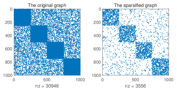
Refer to caption
Refer to caption
Figure 4. Adjacency matrices of an original and sparsifier graph: two experiments.

We have run the experiments with p=0.1p=0.1 and q=0.008q=0.008 for various number n>1n>1 of vertices, e.g. n=1000n=1000 with kk clusters for various k>1k>1, e.g. k=4k=4. In Figure 4, we present two adjacency matrices together with their sparsifiers obtained from UGA for graph sparsifiers with ϵ=0.75\epsilon=0.75. Two experiments are shown with k=4k=4 and n=1000n=1000 that the structure of clusters is well preserved.

Example 4.5.

Next we consider random adjacency matrices and then use our graph sparsification algorithm. Again we use the stochastic block model to generate graphs as in Example 4.4. After permuting the columns and rows of the adjacency matrix AA randomly, we apply a standard spectral clustering method [30] to find clusters with known number of clusters. Also, we first apply the UGA algorithm for graph sparsifiers and then apply the spectral clustering method to find clusters. We demonstrate that the accuracy of clusters obtained from sparsified graph can be better than that from the original graph. Here the accuracy is computed based on the following formula

ci=|Ci∩Ci#|ni,c_{i}=\frac{|C_{i}\cap C_{i}^{\#}|}{n_{i}},

where nin_{i} is the known size of cluster CiC_{i} and Ci#C_{i}^{\#} is the cluster found by the spectral clustering method. Note in our case, C1,⋯,CkC_{1},\cdots,C_{k} are pre-planted index sets and thus are known. We use the average of the accuracies c1,⋯,ckc_{1},\cdots,c_{k} to report the performance of our computation.

In Figure 5, we use n=800n=800 and p=0.08p=0.08 while q=0.008q=0.008, k=4k=4 to generate a graph GG. Then the spectral clustering method to find all clusters of GG using the original adjacency matrix and sparsified adjacency matrix by Algorithm 2. We repeat the experiment 100 times and report the accuracies of clusters for both graphs for each time. The mean of successful rates of finding members of each cluster correctly from the original graphs is 88.73%88.73\% while the mean of successful rates from the sparsified graphs is 93.13%93.13\%. That is, the graph sparsification can improve the accuracy.

Refer to caption
Figure 5. Accuracies in percentage from both graphs over 100100 runs.

4.3. A linear sketching for least squares regression

In many applications in statistical data-analysis and inverse problems, we need to solve a least squares problem. That is, we are given an m×nm\times n matrix AA and an m×1m\times 1 vector 𝐛{\bf b} with m≫nm\gg n. The least squares regression problem is to find an 𝐱o​p​t∈ℝn{\bf x}_{opt}\in\mathbb{R}^{n} such that

(42) 𝐱o​p​t∈arg⁡min𝐱⁡‖A​𝐱−𝐛‖22.{\bf x}_{opt}\in\arg\min_{{\bf x}}\|A{\bf x}-{\bf b}\|^{2}_{2}.

This subsection aims to show that the sparse approximations produced by Algorithm 1 can be useful for least squares regression. Firstly, we consider the case that the coefficient matrix AA is fixed and bb are variable measurements. It has many applications in signal processing and image processing, where AA is a fixed signal sensor with many observations bb. Indeed, for a given

B=A⊤​A=∑i=1m𝐚i⊤​𝐚i,B=A^{\top}A=\sum_{i=1}^{m}{\bf a}_{i}^{\top}{\bf a}_{i},

where A=[𝐚1⊤,⋯,𝐚m⊤]⊤∈ℝm×nA=[{\bf a}_{1}^{\top},\cdots,{\bf a}_{m}^{\top}]^{\top}\in\mathbb{R}^{m\times n} with m≫nm\gg n and for any ϵ>0\epsilon>0, we use Algorithm 1 to find a sparse solution di≥0,i=1,⋯,sd_{i}\geq 0,i=1,\cdots,s with s=O⁡(n/ϵ2)s=O(n/\epsilon^{2}) such that

(43) (1−ϵ)​B≤∑k=1sdk​𝐚jk​𝐚jk⊤≤(1+ϵ)​B.\big(1-\epsilon\big)B\leq\sum_{k=1}^{s}d_{k}{\bf a}_{j_{k}}{\bf a}_{j_{k}}^{\top}\leq\big(1+\epsilon\big)B.

Then we solve A~​𝐱~=𝐛~\tilde{A}\tilde{{\bf x}}=\tilde{{\bf b}} instead of the original least squares problem, where

A~=[d1​𝐚j1ds​𝐚js]​ and ​𝐛~=[bj1bjs].\tilde{A}=\left[\begin{matrix}\sqrt{d_{1}}{\bf a}_{j_{1}}\cr\vdots\cr\sqrt{d_{s}}{\bf a}_{j_{s}}\end{matrix}\right]\hbox{ and }\tilde{{\bf b}}=\left[\begin{matrix}b_{j_{1}}\cr\vdots\cr b_{j_{s}}\end{matrix}\right].

Then we claim that 𝐱~≈𝐱\tilde{{\bf x}}\approx{\bf x} if ‖A⊤​𝐛−A~⊤​𝐛~‖2≈0\|A^{\top}{\bf b}-\tilde{A}^{\top}\tilde{{\bf b}}\|_{2}\approx 0. Indeed, we have the following

Theorem 4.6.

Let 𝐱{\bf x} be the least squares solution satisfying B​𝐱=A⊤​𝐛B{\bf x}=A^{\top}{\bf b} and 𝐱~\tilde{{\bf x}} be the solution A~​𝐱~=𝐛~\tilde{A}\tilde{{\bf x}}=\tilde{{\bf b}} from the above. Suppose that 1−κ⁡(B)​‖B−A~⊤​A~‖2‖B‖2>01-\kappa(B)\frac{\|B-\tilde{A}^{\top}\tilde{A}\|_{2}}{\|B\|_{2}}>0, where κ⁡(B)\kappa(B) stands for the condition number of BB. Then

(44) ‖𝐱−𝐱~‖2‖𝐱‖2≤κ⁡(B)1−κ⁡(B)​‖B−A~⊤​A~‖2‖B‖2​(‖B−A~⊤​A~‖2‖B‖2+‖A⊤​𝐛−A~⊤​𝐛~‖2‖A⊤​𝐛‖2).\frac{\|{\bf x}-\tilde{{\bf x}}\|_{2}}{\|{\bf x}\|_{2}}\leq\frac{\kappa(B)}{1-\kappa(B)\frac{\|B-\tilde{A}^{\top}\tilde{A}\|_{2}}{\|B\|_{2}}}\left(\frac{\|B-\tilde{A}^{\top}\tilde{A}\|_{2}}{\|B\|_{2}}+\frac{\|A^{\top}{\bf b}-\tilde{A}^{\top}\tilde{{\bf b}}\|_{2}}{\|A^{\top}{\bf b}\|_{2}}\right).
Proof.

We mainly use the stability of linear system B​𝐱=A⊤​A​𝐱=A⊤​𝐛B{\bf x}=A^{\top}A{\bf x}=A^{\top}{\bf b} to establish (44). ∎

By (43), we have ‖B−A~⊤​A~‖2=max‖𝐱‖2=1⁡𝐱⊤​(B−A~⊤​A~)​𝐱≤O⁡(ϵ​‖B‖2).\|B-\tilde{A}^{\top}\tilde{A}\|_{2}=\max\limits_{\|{\bf x}\|_{2}=1}{\bf x}^{\top}(B-\tilde{A}^{\top}\tilde{A}){\bf x}\leq O(\epsilon\|B\|_{2}). If ‖A⊤​𝐛−A~⊤​𝐛~‖2→0\|A^{\top}{\bf b}-\tilde{A}^{\top}\tilde{{\bf b}}\|_{2}\to 0, then the right-hand side of (44) is very small, and hence, the approximating solution 𝐱~\tilde{{\bf x}} is close to the true solution 𝐱{\bf x}.

Such a computational method is similar to the linear sketching approach discussed in [7, 29, 43] by compressing the data AA and 𝐛{\bf b} as small as possible before doing linear regression. So our Algorithm 1 provides another approach for linear sketching. Instead of using the linear sketching method to find 𝐲=A~\𝐛~{\bf y}=\tilde{A}\backslash\tilde{{\bf b}} we propose to solve 𝐳=(A~)⊤​A~\A⊤​𝐛{\bf z}=(\tilde{A})^{\top}\tilde{A}\backslash A^{\top}{\bf b} directly. The reason for this new solution can be seen from (44) that the solution will make the second term on the right-hand side to be zero. In the following example, we compare two solutions to demonstrate numerically that our new method is more accurate.

Example 4.7.

We use Algorithm 1 to find a linear sketching A~\tilde{A} and 𝐛~\tilde{{\bf b}} with various ϵ∈(0,1)\epsilon\in(0,1). Once we find the linear sketching, we repeatedly solve a linear squares regression by using the linear sketching method: 𝐲=A~\𝐛~{\bf y}=\tilde{A}\backslash\tilde{{\bf b}} and our new method over 100100 times and compute the averaged times and errors. Let Time-LS, Time-New and Time-O denote the computational times for the two methods as well as the method using Matlab backslash, i.e. 𝐱=A\𝐛{\bf x}=A\backslash{\bf b}, respectively. We use RE-LS to denote the averaged relative residual error, i.e. ‖𝐲−𝐱‖2/‖𝐱‖2\|{\bf y}-{\bf x}\|_{2}/\|{\bf x}\|_{2} by the linear sketching solution method. Similarly, RE-New denotes the relative residual error, ‖𝐳−𝐱‖2/‖𝐱‖2\|{\bf z}-{\bf x}\|_{2}/\|{\bf x}\|_{2}. In Table 2, we use n=300,m=90000n=300,m=90000.

Table 2. Performance of the linear sketching method and our new method
ϵ\epsilon RE-LS RE-New Time-O Time-LS Time-New BE
0.90 2.7487 15.5786 2.5359 0.0013 0.0123 2
0.80 2.0325 4.6479 2.7808 0.0014 0.0130 2
0.70 1.7395 2.1582 2.7758 0.0014 0.0127 2
0.60 1.5517 1.1918 2.6825 0.0017 0.0130 3
0.50 1.4372 0.6701 2.6087 0.0020 0.0128 6
0.40 1.3603 0.3807 2.7778 0.0023 0.0132 7
0.30 1.2931 0.2045 2.6791 0.0026 0.0121 14
0.20 1.1968 0.0917 2.7881 0.0028 0.0140 29

The numbers in the last column are the numbers of the columns in the right-hand side of the least squares problem to break even (BE) of the computational time of our new method with Matlab least squares method, i.e. 𝐱=A\𝐛{\bf x}=A\backslash{\bf b}. That is, if there are 3030 columns or more on the right-hand side of least squares regression, we should use Algorithm 1 to find A~\tilde{A} and use our new method to solve them with ϵ=0.2\epsilon=0.2.

References

  • [1] E. Abbe, Community detection and stochastic block models: Recent developments, Foundations and Trends in Communications and Information Theory, 14 (2017), pp. 1–162.
  • [2] Z. Allen-Zhu, Z. Liao, and L. Orecchia, Spectral sparsification and regret minimization beyond matrix multiplicative updates, in Proceedings of the 47th Annual ACM Symposium on Theory of Computing, 2015, pp. 237–245.
  • [3] N. Bansal, O. Svensson, and L. Trevisan, New notions and constructions of sparsification for graphs and hypergraphs, in 2019 IEEE 60th Annual Symposium on Foundations of Computer Science (FOCS), IEEE, 2019, pp. 910–928.
  • [4] J. Batson, D. A. Spielman, and N. Srivastava, Twice-Ramanujan sparsifiers, SIAM Review, 56 (2014), pp. 315–334.
  • [5] J. Batson, D. A. Spielman, N. Srivastava, and S.-H. Teng, Spectral sparsification of graphs: Theory and algorithms, Communications of the ACM, 56 (2013), pp. 87–94.
  • [6] A. A. Benczúr and D. R. Karger, Approximating ss-tt minimum cuts in O⁡(n2)O(n^{2}) time, in Proceedings of the 28th annual ACM Symposium on Theory of Computing, 1996, pp. 47–55.
  • [7] C. Boutsidis, P. Drineas, and M. Magdon-Ismail, Near-optimal coresets for least-squares regression, IEEE Trans. Inform. Theory, 59 (2013), pp. 6880–6892.
  • [8] T. Chu, Y. Gao, R. Peng, S. Sachdeva, S. Sawlani, and J. Wang, Graph sparsification, spectral sketches, and faster resistance computation via short cycle decompositions, SIAM J. Comput., (2020), pp. FOCS18–85.
  • [9] F. Chung and M. Radcliffe, On the spectra of general random graphs, The Electronic Journal of Combinatorics, (2011), pp. P215–P215.
  • [10] J. Chuzhoy, Y. Gao, J. Li, D. Nanongkai, R. Peng, and T. Saranurak, A deterministic algorithm for balanced cut with applications to dynamic connectivity, flows, and beyond, preprint arXiv:1910.08025, (2019).
  • [11] A. Cohen, W. Dahmen, and R. DeVore, Orthogonal matching pursuit under the restricted isometry property, Constr. Approx., 45 (2017), pp. 113–127.
  • [12] R. A. Devore and V. N. Temlyakov, Some remarks on greedy algorithms, Adv. Comput. Math., 5 (1996), pp. 173–187.
  • [13] D. L. Donoho, Compressed sensing, IEEE Trans. Inform. Theory, 52 (2006), pp. 1289–1306.
  • [14] D. L. Donoho and J. Tanner, Sparse nonnegative solution of underdetermined linear equations by linear programming, Proceedings of the National Academy of Sciences, 102 (2005), pp. 9446–9451.
  • [15] Z. Feng, Spectral graph sparsification in nearly-linear time leveraging efficient spectral perturbation analysis, in Proceedings of the 53rd Annual Design Automation Conference, 2016, pp. 1–6.
  • [16] Z. Feng, Similarity-aware spectral sparsification by edge filtering, in 2018 55th ACM/ESDA/IEEE Design Automation Conference (DAC), IEEE, 2018, pp. 1–6.
  • [17] S. Foucart and D. Koslicki, Sparse recovery by means of nonnegative least squares, IEEE Signal Process. Lett., 21 (2014), pp. 498–502.
  • [18] S. Foucart and H. Rauhut, A mathematical introduction to compressive sensing, 2013.
  • [19] O. Friedland and P. Youssef, Approximating matrices and convex bodies, Int. Math. Res. Not., 2019 (2019), pp. 2519–2537.
  • [20] A. Frieze and M. Karoński, Introduction to random graphs, Cambridge University Press, 2016.
  • [21] G. B. Hermsdorff and L. Gunderson, A unifying framework for spectrum-preserving graph sparsification and coarsening, in Advances in Neural Information Processing Systems, 2019, pp. 7736–7747.
  • [22] A. Jambulapati and A. Sidford, Efficient O~​(n/ϵ)\tilde{O}(n/\epsilon) spectral sketches for the laplacian and its pseudoinverse, in Proceedings of the 29th Annual ACM-SIAM Symposium on Discrete Algorithms, SIAM, 2018, pp. 2487–2503.
  • [23] R. Kyng, Y. T. Lee, R. Peng, S. Sachdeva, and D. A. Spielman, Sparsified cholesky and multigrid solvers for connection laplacians, in Proceedings of the 48th Annual ACM Symposium on Theory of Computing, 2016, pp. 842–850.
  • [24] R. Kyng, J. Pachocki, R. Peng, and S. Sachdeva, A framework for analyzing resparsification algorithms, in Proceedings of the 28th Annual ACM-SIAM Symposium on Discrete Algorithms, SIAM, 2017, pp. 2032–2043.
  • [25] M.-J. Lai and D. Mckenzie, Compressive sensing for cut improvement and local clustering, SIAM J. Math. Data Sciences, 2 (2020), pp. 368–395.
  • [26] Y. T. Lee and H. Sun, An SDP-based algorithm for linear-sized spectral sparsification, in In 49th Annual ACM Symposium on Theory of Computing, 2017, pp. 678–687.
  • [27] Y. T. Lee and H. Sun, Constructing linear-sized spectral sparsification in almost-linear time, SIAM J. Comput., 47 (2018), pp. 2315–2336.
  • [28] H. Li, R. Peng, L. Shan, Y. Yi, and Z. Zhang, Current flow group closeness centrality for complex networks, in The World Wide Web Conference, 2019, pp. 961–971.
  • [29] L. Mor-Yosef and H. Avron, Sketching for principal component regression, SIAM J. Matrix Anal. Appl., 40 (2019), pp. 454–485.
  • [30] A. Ng, M. Jordan, and Y. Weiss, On spectral clustering: Analysis and an algorithm, Advances in Neural Information Processing Systems, 14 (2001), pp. 849–856.
  • [31] Y. C. Pati, R. Rezaiifar, and P. S. Krishnaprasad, Orthogonal matching pursuit: Recursive function approximation with applications to wavelet decomposition, in Proceedings of 27th Asilomar Conference on Signals, Systems and Computers, IEEE, 1993, pp. 40–44.
  • [32] M. Silva, N. Harvey, and C. M. Sato, Sparse sums of positive semidefinite matrices, ACM Transactions on Algorithms (TALG), 12 (2015), pp. 1–17.
  • [33] D. A. Spielman, Spectral and algebraic graph theory, 2019. http://cs-www.cs.yale.edu/homes/spielman/sagt/.
  • [34] D. A. Spielman and N. Srivastava, Graph sparsification by effective resistances, SIAM J. Comput., 40 (2011), pp. 1913–1926.
  • [35] D. A. Spielman and S.-H. Teng, Spectral sparsification of graphs, SIAM J. Comput., 40 (2011), pp. 981–1025.
  • [36] D. A. Spielman and S.-H. Teng, Nearly linear time algorithms for preconditioning and solving symmetric, diagonally dominant linear systems, SIAM J. Matrix Anal. Appl., 35 (2014), pp. 835–885.
  • [37] S.-H. Teng, Scalable algorithms for data and network analysis, Found. Trends Theor. Comput. Sci., 12 (2016), pp. 1–274.
  • [38] J. A. Tropp, Greed is good: Algorithmic results for sparse approximation, IEEE Trans. Inform. theory, 50 (2004), pp. 2231–2242.
  • [39] J. A. Tropp and A. C. Gilbert, Signal recovery from random measurements via orthogonal matching pursuit, IEEE Trans. Inform. Theory, 53 (2007), pp. 4655–4666.
  • [40] N. K. Vishnoi, Lx=b. Laplacian solvers and their algorithmic applications, Found. Trends Theor. Comput. Sci., 8 (2013), pp. 1–141.
  • [41] Z. Wang, M. J. Lai, Z. Lu, W. Fan, H. Davulcu, and J. Ye, Rank-one matrix pursuit for matrix completion, in International Conference on Machine Learning, 2014, pp. 91–99.
  • [42] Z. Wang, M. J. Lai, Z. Lu, W. Fan, H. Davulcu, and J. Ye, Orthogonal rank-one matrix pursuit for low rank matrix completion, SIAM J. Sci. Comput., 37 (2015), pp. A488–A514.
  • [43] D. P. Woodruff, Sketching as a tool for numerical linear algebra, Found. Trends Theor. Comput. Sci., 10 (2014), pp. 1–157.
  • [44] H. Wu and Y. Chen, Graph sparsification with generative adversarial network, preprint arXiv: 2009.11736, (2020).
  • [45] Z. Xu, The performance of orthogonal multi-matching pursuit under RIP, J. Comp. Math., 33 (2015), pp. 495–516.
  • [46] T. Zhang, Sparse recovery with orthogonal matching pursuit under RIP, IEEE Trans. Inform. Theory, 57 (2011), pp. 6215–6221.
  • [47] Y. Zhang, Z. Zhao, and Z. Feng, SF-GRASS: Solver-free graph spectral sparsification, in 2020 IEEE/ACM International Conference On Computer Aided Design (ICCAD), 2020, pp. 1–8.
  • [48] Z. Zhao, Y. Wang, and Z. Feng, Nearly-linear time spectral graph reduction for scalable graph partitioning and data visualization, preprint arXiv:1812.08942, (2018).
  • [49] A. Zouzias, A matrix hyperbolic cosine algorithm and applications, in International Colloquium on Automata, Languages, and Programming, 2012, pp. 846–858.