PrivColl: Practical Privacy-Preserving Collaborative Machine Learning

Gradient descent is by far the most commonly used optimization strategy among various machine learning and deep learning algorithms. It is used to find the values of coefficients that minimize a cost function as far as possible. Given a defined cost function $J$, the coefficient matrix $W$ is derived by the optimization $\argmin_{W}J$, and is updated as:

Given a particular training dataset $X$ and a label matrix $y$, the cost function $J$ can be defined as $J(\sigma(XW),y,W)$, where $\sigma$ is determined by the learning model. For example, in logistic regression, $\sigma$ is usually a sigmoid function $1/(1+e^{-z})$, while in neural network, $\sigma$ is a composite function that is known as forward propagation. According to the chain rule in calculus, the gradient with respect to $W$ is computed as $\frac{\partial{J}}{\partial{\sigma}}\frac{\partial{\sigma}}{\partial{XW}}\frac{\partial{XW}}{\partial{W}}+\tau$, where $\tau$ is the gradient with respect to the regularization term, which is independent to $X$. Let $\Delta$ be $\frac{\partial{J}}{\partial{\sigma}}\frac{\partial{\sigma}}{\partial{XW}}$, and $\frac{\partial{XW}}{\partial{W}}$ equals to $X$, then the gradient with respect to $W$ can be written as:

As such, we can decompose the gradient descent optimization into $\Delta$ , $X$ and $\tau$, in which $\Delta$ is a function of $XW$. This provides an algorithmic foundation for PrivColl’s distribution of learning algorithms.

Secret sharing schemes aim to securely distribute secret values amongst a group of participants. PrivColl employs the secret sharing scheme proposed by [4], which uses additive sharing over $\mathbb{Z}_{2^{32}}$. In this scheme, a secret value $srt$ is split to $s$ shares $E^{1}_{srt},...,E^{s}_{srt}\in\mathbb{Z}_{2^{32}}$ such that

and any $s-1$ elements $E^{i_{1}}_{srt},...,E^{i_{s-1}}_{srt}$ are uniformly distributed. This prevents any participant who has part of the shares from deriving the value of $srt$, unless all participants join their shares.

In addition, the scheme has a homomorphic property that allows efficient and secure addition on a set of secret values $srt_{1},...,srt_{s}$ held by corresponding participants $S_{1},...,S_{s}$. To do this, each participant $S_{i}$ executes a randomised sharing algorithm $Shr(srt_{i},S)$ to split its secret $srt_{i}$ into shares $E^{1}_{srt_{i}},...,E^{s}_{srt_{i}}$, and distributes each $E^{j}_{srt_{i}}$ to the participant $S_{j}$. Then, each $S_{i}$ locally adds the shares it holds, $E^{i}_{srt_{1}},...,E^{i}_{srt_{s}}$, to produce $\sum_{j=1}^{s}E^{i}_{srt_{j}}$ (denoted by $E^{i}$ for brevity). After that, a reconstruction algorithm $Rec(\{(E^{i},S_{i})\}_{S_{i}\in S})$, which takes $E^{i}$ from each participant and add them together, can be executed by an aggregator to reconstruct the $\sum_{i=1}^{s}srt_{i}$ without revealing any secret addends $srt_{i}$.

The involved parties in PrivColl are a set of local nodes (i.e., data owners) $S_{1},...,S_{s}$ and an aggregation node $Agg$. Each local node holds part of features of the training samples, denoted by $X^{l}$ $(l\in\{1,...,s\})$, and the corresponding local model $W^{l}$ $(l\in\{1,...,s\})$ trained on $X^{l}$. Each $X^{l}\in\mathbb{R}^{m\times d_{l}}$ is a $m\times d_{l}$ matrix representing $m$ training samples with $d_{l}$ features, and $W^{l}\in\mathbb{R}^{d_{l}\times k}$ is a matrix of coefficients, where $k$ is the number of output classes. In PrivColl, $m$ and $k$ are public and known by every party, and $d_{l}$ is private and only known by the corresponding data owner $S_{l}$. We use $X$ to denote the vertical concatenation of the local training datasets $X^{1},...,X^{s}$. Then we know that $X$ is a $m\times n$ matrix where $n=\sum_{l=1}^{s}d_{l}$ (i.e., the total number of features in $X$). Since $d_{l}$ is private, $n$ is unknown unless all of the local nodes join their views.

PrivColl aims to defend against an honest-but-curious adversary $\mathcal{A}$, who follows the collaboration protocols and training procedures, but is intending to obtain the datasets of other local nodes (i.e., $X^{l}$) and/or the model parameters trained out of them (i.e., $W^{l}$). The adversary may control $Agg$, and $t$ out of $s$ local nodes. Here, we conservatively assume $t<s-1$, which implies that at least two local nodes need to be out of the adversary’s control, as $s-1$ comprised local nodes who has the sum of their shares, colluding with $Agg$ who has the sum of all shares, will be able to obtain the share of the remaining node by a simple subtraction (detailed in Section 4).

Keeping local data/model private and providing functional correctness are the main properties PrivColl aims to achieve. Below we present the definitions of these two properties.

Figure 1 illustrates the end-to-end workflow of PrivColl, which is divided into the following steps.

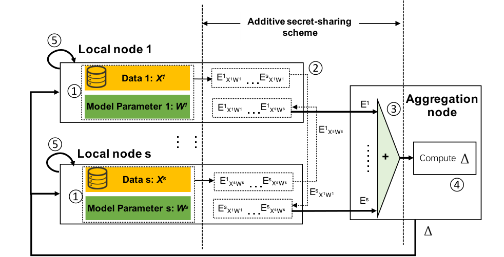
Initialization: Each local node $S_{l}$ holds its own training dataset $X^{l}\in\mathbb{R}^{m\times d_{l}}$, and randomly initializes its coefficient matrix $W^{l}\in\mathbb{R}^{d_{l}\times k}$.

Step 1: In each iteration of gradient descent, each $S_{l}$ multiplies $X^{l}$ by $W^{l}$ locally, resulting in a $X^{l}W^{l}\in\mathbb{R}^{m\times k}$. The value of $d_{l}$, i.e., the number of features in $X^{l}$, is removed by such a matrix multiplication.

Step 2: Each $S_{l}$ executes the sharing algorithm $Shr$ to split $X^{l}W^{l}$ into $s$ shares using the additive secret sharing scheme.

in which $Shr$ takes as input a secret $X^{l}W^{l}$ and a set $S$ of local nodes, and produces a set of shares $E^{i}_{X^{l}W^{l}}(i\in\{1,...,s\})$, each of which is distributed to a different $S_{i}\in S$. Then, each $S_{l}$ calculates the sum of all shares it receives, and gets $E^{l}=\sum_{j=1}^{s}E_{X^{j}W^{j}}^{l}$.

Step 3: $Agg$ collects all $E^{l}$ from local nodes and add them together. Since

this addition reconstructs the homomorphic addition result $XW$ (equals $\sum\limits_{l=1}^{s}X^{l}W^{l}$).

Step 4: $Agg$ computes $\Delta=\frac{\partial{J}}{\partial{\sigma}}\frac{\partial{\sigma}}{\partial{XW}}$ (c.f., Equation 2), and sends $\Delta$ back to the local nodes.

Step 5: With the received $\Delta$, each $S_{l}$ updates its local coefficient matrix $W^{l}$.

Step 1-5 are repeated for the next training iteration until convergence.

We start with the following lemma that is soon used in our proof.

We define the party knowledge as the overall knowledge that can be learned by adversary parties. It includes the parties’ own inputs, and the additional knowledge that can be inferred from the training iterations. We prove that the party knowledge in PrivColl is bounded within a certain range. In particular, we demonstrate that the overall party knowledge of adversary party $I$ in PrivColl is a set of $\{X^{l^{\prime}}\mid_{l^{\prime}\in I},W^{l^{\prime}}\mid_{l^{\prime}\in I},XW,\sum X^{l}W^{l}\mid_{l\in S\setminus I},\sum X^{l}(X^{l})^{T}\mid_{l\in S\setminus I},XX^{T}\}$, where $\{X^{l^{\prime}}\mid_{l^{\prime}\in I},W^{l^{\prime}}\mid_{l^{\prime}\in I},XW\}$ are the adversary’s own input in the workflow, and $\{\sum X^{l}W^{l}\mid_{l\in S\setminus I},\sum X^{l}(X^{l})^{T}\mid_{l\in S\setminus I},XX^{T}\}$ are the additional information that can be inferred from the training iterations. The party knowledge we derive in this Section will be used in Section 4.3 to prove the privacy preservation of PrivColl.

We use the simulation paradigm (also known as the real/ideal model) [15] to prove such a bound of party knowledge. The simulation paradigm compares what an adversary can do in a real protocol execution $REAL$ to what it can do in an ideal setting with a trusted functionality (simulation) $SIM$ [15]. Formally, the protocol $\mathcal{P}$ securely computes a functionality $\mathcal{F}_{\mathcal{P}}$ if for every adversary in $REAL$, there exists an adversary in $SIM$, such that the view of the adversary from $REAL$ is indistinguishable from the view of the adversary from $SIM$. A perfect indistinguishability [6] between the view of $REAL$ and $SIM$ guarantees that the adversary, without error probability, can learn nothing more than their own inputs and the information required by $SIM$ for the simulation.

We introduce some notations used in our proof. We use $X^{S^{\prime}}=\{X^{l}|S_{l}\in S^{\prime}\}$ to indicate the inputs of any subset of local nodes $S^{\prime}\subseteq S$. Given any subset $I_{0}\subseteq S$ of the parties without the knowledge of $XW$, and subset $I_{1}\subseteq S\cup\{Agg\}$ of the parties with the knowledge of $XW$, let $REAL(X^{S},XW,S,t,\mathcal{P},I)$ denote the combined views of all parties in $I=I_{0}\cup I_{1}$ from the execution of a real protocol $\mathcal{P}$, where $t$ is the adversary threshold (recall that $t<s-1$). Let $SIM(X^{I},Z,S,t,\mathcal{F}_{\mathcal{P}},I)$ denote the views of $I$ from an ideal execution, where $Z$ is the information required by $SIM$ for the simulation. In other words, the $Z$ indicates the party knowledge that the adversary can and only can learn other than their own inputs.

With lemma introduced in Section 4.1, and party knowledge discussed in Section 4.2, we give our theorem of privacy preservation guarantee.

With Theorem 4.2, we demonstrate that, with a sufficient rank of the training dataset of honest parties, e.g. $\geq$ 35, which is common in real-world datasets, PrivColl achieves $10^{-40}$-privacy.

The following theorem demonstrates that if a non-distributed gradient descent optimization algorithm taking $X$ as input, denoted by $\mathcal{F}_{GD}(X)$, converges to a local/global minima $\eta$, then executing PrivColl with the same hyper settings (such as cost function, step size, and model structure) on $X^{1},...,X^{s}$, denoted by $\mathcal{F}^{\prime}_{GD}(\{(S_{l},X^{l}),Agg\}_{S_{l}\in S})$, also converges to $\eta$.

Figure 2 shows an example of a two-layer feed-forward recurrent neural network (RNN). Every neural layer is attached with a time subscript $c$. The weight matrix $W$ maps the input vector $X^{(c)}$ to the hidden layer $h^{(c)}$. The weight matrix $V$ propagates the hidden layer to the output layer $\hat{y}^{(c)}$. The weight matrix $U$ maps the previous hidden layer to the current one.

References

- [1] Abadi, M., Chu, A., Goodfellow, I., McMahan, H.B., Mironov, I., Talwar, K., Zhang, L.: Deep learning with differential privacy. In: Proceedings of the 2016 ACM SIGSAC Conference on Computer and Communications Security. pp. 308–318 (2016)
- [2] Abuadbba, S., Kim, K., Kim, M., Thapa, C., Camtepe, S.A., Gao, Y., Kim, H., Nepal, S.: Can we use split learning on 1d cnn models for privacy preserving training? arXiv preprint arXiv:2003.12365 (2020)
- [3] Albrecht, M., Chase, M., Chen, H., Ding, J., Goldwasser, S., Gorbunov, S., Halevi, S., Hoffstein, J., Laine, K., Lauter, K., Lokam, S., Micciancio, D., Moody, D., Morrison, T., Sahai, A., Vaikuntanathan, V.: Homomorphic encryption security standard. Tech. rep., HomomorphicEncryption.org (2018)
- [4] Bogdanov, D., Laur, S., Willemson, J.: Sharemind: A framework for fast privacy-preserving computations. In: European Symposium on Research in Computer Security. pp. 192–206. Springer (2008)
- [5] Bonawitz, K., Ivanov, V., Kreuter, B., Marcedone, A., McMahan, H.B., Patel, S., Ramage, D., Segal, A., Seth, K.: Practical secure aggregation for privacy-preserving machine learning. In: Proceedings of the 2017 ACM SIGSAC Conference on Computer and Communications Security. pp. 1175–1191. ACM (2017)
- [6] Canetti, R.: Theory of cryptography. Springer (2008)
- [7] Chen, Y.R., Rezapour, A., Tzeng, W.G.: Privacy-preserving ridge regression on distributed data. Information Sciences 451, 34–49 (2018)
- [8] Dwork, C., Roth, A., et al.: The algorithmic foundations of differential privacy. Foundations and Trends® in Theoretical Computer Science 9(3–4), 211–407 (2014)
- [9] Esposito, C., Su, X., Aljawarneh, S.A., Choi, C.: Securing collaborative deep learning in industrial applications within adversarial scenarios. IEEE Transactions on Industrial Informatics 14(11), 4972–4981 (2018)
- [10] Fredrikson, M., Jha, S., Ristenpart, T.: Model inversion attacks that exploit confidence information and basic countermeasures. In: Proceedings of the 22nd ACM SIGSAC Conference on Computer and Communications Security. pp. 1322–1333 (2015)
- [11] Gascón, A., Schoppmann, P., Balle, B., Raykova, M., Doerner, J., Zahur, S., Evans, D.: Secure linear regression on vertically partitioned datasets. IACR Cryptology ePrint Archive 2016, 892 (2016)
- [12] Gascón, A., Schoppmann, P., Balle, B., Raykova, M., Doerner, J., Zahur, S., Evans, D.: Privacy-preserving distributed linear regression on high-dimensional data. Proceedings on Privacy Enhancing Technologies 2017(4), 345–364 (2017)
- [13] Gentry, C.: Fully homomorphic encryption using ideal lattices. In: Proceedings of the forty-first annual ACM symposium on Theory of computing. pp. 169–178 (2009)
- [14] Gilad-Bachrach, R., Dowlin, N., Laine, K., Lauter, K., Naehrig, M., Wernsing, J.: Cryptonets: Applying neural networks to encrypted data with high throughput and accuracy. In: International Conference on Machine Learning. pp. 201–210 (2016)
- [15] Goldreich, O., Micali, S., Wigderson, A.: How to play any mental game, or a completeness theorem for protocols with honest majority. In: Providing Sound Foundations for Cryptography: On the Work of Shafi Goldwasser and Silvio Micali, pp. 307–328 (2019)
- [16] Golub, G., Van Loan, C.: Matrix computations 3rd edition the john hopkins university press. Baltimore, MD (1996)
- [17] Guennebaud, G., Jacob, B., et al.: Eigen v3. http://eigen.tuxfamily.org (2010)
- [18] Gupta, O., Raskar, R.: Distributed learning of deep neural network over multiple agents. Journal of Network and Computer Applications 116, 1–8 (2018)
- [19] Hagestedt, I., Zhang, Y., Humbert, M., Berrang, P., Tang, H., Wang, X., Backes, M.: Mbeacon: Privacy-preserving beacons for dna methylation data. In: NDSS (2019)
- [20] Hardy, S., Henecka, W., Ivey-Law, H., Nock, R., Patrini, G., Smith, G., Thorne, B.: Private federated learning on vertically partitioned data via entity resolution and additively homomorphic encryption. arXiv preprint arXiv:1711.10677 (2017)
- [21] Hintjens, P.: ZeroMQ: messaging for many applications. ” O’Reilly Media, Inc.” (2013)
- [22] Horn, R.A., Johnson, C.R.: Matrix analysis. Cambridge university press (2012)
- [23] Hu, Y., Niu, D., Yang, J., Zhou, S.: Fdml: A collaborative machine learning framework for distributed features. In: Proceedings of the 25th ACM SIGKDD International Conference on Knowledge Discovery & Data Mining. pp. 2232–2240 (2019)
- [24] Jia, Q., Guo, L., Jin, Z., Fang, Y.: Privacy-preserving data classification and similarity evaluation for distributed systems. In: 2016 IEEE 36th International Conference on Distributed Computing Systems (ICDCS). pp. 690–699. IEEE (2016)
- [25] Ko, R.K., Russello, G., Nelson, R., Pang, S., Cheang, A., Dobbie, G., Sarrafzadeh, A., Chaisiri, S., Asghar, M.R., Holmes, G.: Stratus: Towards returning data control to cloud users. In: International Conference on Algorithms and Architectures for Parallel Processing. pp. 57–70. Springer (2015)
- [26] Kwabena, O.A., Qin, Z., Zhuang, T., Qin, Z.: Mscryptonet: Multi-scheme privacy-preserving deep learning in cloud computing. IEEE Access 7, 29344–29354 (2019)
- [27] LeCun, Y., Cortes, C.: MNIST handwritten digit database (2010), http://yann.lecun.com/exdb/mnist/
- [28] Liu, J., Juuti, M., Lu, Y., Asokan, N.: Oblivious neural network predictions via minionn transformations. In: Proceedings of the 2017 ACM SIGSAC Conference on Computer and Communications Security. pp. 619–631 (2017)
- [29] Marc, T., Stopar, M., Hartman, J., Bizjak, M., Modic, J.: Privacy-enhanced machine learning with functional encryption. In: European Symposium on Research in Computer Security. pp. 3–21. Springer (2019)
- [30] Melis, L., Song, C., De Cristofaro, E., Shmatikov, V.: Exploiting unintended feature leakage in collaborative learning. In: 2019 IEEE Symposium on Security and Privacy (SP). pp. 691–706. IEEE (2019)
- [31] Mohassel, P., Zhang, Y.: Secureml: A system for scalable privacy-preserving machine learning. In: 2017 IEEE Symposium on Security and Privacy (SP). pp. 19–38. IEEE (2017)
- [32] Papernot, N., McDaniel, P., Sinha, A., Wellman, M.: Towards the science of security and privacy in machine learning. arXiv preprint arXiv:1611.03814 (2016)
- [33] Papernot, N., Song, S., Mironov, I., Raghunathan, A., Talwar, K., Erlingsson, Ú.: Scalable private learning with pate. arXiv preprint arXiv:1802.08908 (2018)
- [34] Ryffel, T., Trask, A., Dahl, M., Wagner, B., Mancuso, J., Rueckert, D., Passerat-Palmbach, J.: A generic framework for privacy preserving deep learning. arXiv preprint arXiv:1811.04017 (2018)
- [35] Sadat, M.N., Aziz, M.M.A., Mohammed, N., Chen, F., Wang, S., Jiang, X.: Safety: Secure gwas in federated environment through a hybrid solution with intel sgx and homomorphic encryption. arXiv preprint arXiv:1703.02577 (2017)
- [36] Sharma, S., Chen, K.: Confidential boosting with random linear classifiers for outsourced user-generated data. In: European Symposium on Research in Computer Security. pp. 41–65. Springer (2019)
- [37] Shokri, R., Shmatikov, V.: Privacy-preserving deep learning. In: Proceedings of the 22nd ACM SIGSAC conference on computer and communications security. pp. 1310–1321 (2015)
- [38] Song, S., Chaudhuri, K., Sarwate, A.D.: Stochastic gradient descent with differentially private updates. In: 2013 IEEE Global Conference on Signal and Information Processing. pp. 245–248. IEEE (2013)
- [39] Vepakomma, P., Gupta, O., Swedish, T., Raskar, R.: Split learning for health: Distributed deep learning without sharing raw patient data. arXiv preprint arXiv:1812.00564 (2018)
- [40] Wang, S., Pi, A., Zhou, X.: Scalable distributed dl training: Batching communication and computation. In: Proceedings of the AAAI Conference on Artificial Intelligence. vol. 33, pp. 5289–5296 (2019)
- [41] Will, M.A., Nicholson, B., Tiehuis, M., Ko, R.K.: Secure voting in the cloud using homomorphic encryption and mobile agents. In: 2015 International Conference on Cloud Computing Research and Innovation (ICCCRI). pp. 173–184. IEEE (2015)
- [42] Yao, A.C.C.: How to generate and exchange secrets. In: 27th Annual Symposium on Foundations of Computer Science (sfcs 1986). pp. 162–167. IEEE (1986)
- [43] Yuan, J., Yu, S.: Privacy preserving back-propagation neural network learning made practical with cloud computing. IEEE Transactions on Parallel and Distributed Systems 25(1), 212–221 (2014)
- [44] Zhang, J., Chen, B., Yu, S., Deng, H.: Pefl: A privacy-enhanced federated learning scheme for big data analytics. In: 2019 IEEE Global Communications Conference (GLOBECOM). pp. 1–6. IEEE (2019)
- [45] Zhang, X., Ji, S., Wang, H., Wang, T.: Private, yet practical, multiparty deep learning. In: 2017 IEEE 37th International Conference on Distributed Computing Systems (ICDCS). pp. 1442–1452. IEEE (2017)
- [46] Zhang, Y., Bai, G., Zhong, M., Li, X., Ko, R.: Differentially private collaborative coupling learning for recommender systems. IEEE Intelligent Systems (2020)
- [47] Zhang, Y., Zhao, X., Li, X., Zhong, M., Curtis, C., Chen, C.: Enabling privacy-preserving sharing of genomic data for gwass in decentralized networks. In: Proceedings of the Twelfth ACM International Conference on Web Search and Data Mining. pp. 204–212. ACM (2019)
- [48] Zheng, H., Ye, Q., Hu, H., Fang, C., Shi, J.: Bdpl: A boundary differentially private layer against machine learning model extraction attacks. In: European Symposium on Research in Computer Security. pp. 66–83. Springer (2019)
- [49] Zheng, Y., Duan, H., Wang, C.: Towards secure and efficient outsourcing of machine learning classification. In: European Symposium on Research in Computer Security. pp. 22–40. Springer (2019)