Theoretical investigation of twin boundaries in WO₃: Structure, properties and implications for superconductivity

Tungsten trioxide, $\text{WO}{\vphantom{\text{X}}}_{\smash[t]{\text{3}}}$, is a functionally versatile material with possible applications based on electrochromism (smart windows), gasochromism (gas sensors) and photocatalysis Granqvist 2000; Zheng et al. 2011; Santato et al. 2001. The high-symmetry structure of $\text{WO}{\vphantom{\text{X}}}_{\smash[t]{\text{3}}}$ is that of a perovskite with a vacant A site (see Fig. 1), and it exhibits a series of lower symmetry phases at lower temperature. Both its structure and its properties depend on and can be tuned by doping Hagenmuller 1973. For instance, while pure $\text{WO}{\vphantom{\text{X}}}_{\smash[t]{\text{3}}}$ is an insulator, it becomes metallic upon occupation of the A sites with alkali metal ions. In addition, superconductivity was reported as early as 1964 for Na-doped $\text{WO}{\vphantom{\text{X}}}_{\smash[t]{\text{3}}}$, and $\text{M}{\vphantom{\text{X}}}_{\smash[t]{\text{x\/}}}\text{WO}{\vphantom{\text{X}}}_{\smash[t]{\text{3\hskip 0.90417pt--\hskip 0.90417ptx\/}}}$ systems are now well established as superconductors (with M usually an alkali metal) Raub et al. 1964; Sweedler et al. 1965a; Sweedler et al. 1965b; Hubble et al. 1971; Shanks 1974; Skokan et al. 1979; Cadwell et al. 1981; Garif’yanov et al. 1996; Salje et al. 1997; Brusetti et al. 2002; Reich et al. 2009; Bocarsly et al. 2013; Haldolaarachchige et al. 2014a. The reported superconducting critical temperatures ($T_{c}$) for bulk $\text{M}{\vphantom{\text{X}}}_{\smash[t]{\text{x\/}}}\text{WO}{\vphantom{\text{X}}}_{\smash[t]{\text{3\hskip 0.90417pt--\hskip 0.90417ptx\/}}}$ systems are generally less than $2\text{\,}\mathrm{K}$ Shanks 1974; Garif’yanov et al. 1996, and, interestingly, tend to decrease with increasing doping above the lowest doping level at which superconductivity is observed Shanks 1974; Haldolaarachchige et al. 2014b; Pellegrini et al. 2019. Moreover, different dopants result in superconductivity in different structural phases. More recently, non-bulk high-temperature superconductivity was reported on the surface of dopant-rich islands in $\text{Na}{\vphantom{\text{X}}}_{\smash[t]{\text{x\/}}}\text{WO}{\vphantom{\text{X}}}_{\smash[t]{\text{3\hskip 0.90417pt--\hskip 0.90417ptx\/}}}$ Reich and Tsabba 1999. Around the same time, superconductivity was discovered in reduced $\text{WO}{\vphantom{\text{X}}}_{\smash[t]{\text{3\hskip 0.90417pt--\hskip 0.90417ptx\/}}}$ with a superconducting critical temperature of around $3\text{\,}\mathrm{K}$ Aird et al. 1998; Aird and Salje 1998; Aird and Salje 2000. In this case, the bulk sample was not superconducting, but sheet superconductivity occurred along the ferroelastic domain walls of the reduced $\text{WO}{\vphantom{\text{X}}}_{\smash[t]{\text{3\hskip 0.90417pt--\hskip 0.90417ptx\/}}}$ crystals.

At room temperature, $\text{WO}{\vphantom{\text{X}}}_{\smash[t]{\text{3}}}$ shows two types of ferroelastic domain walls which correspond to two successive ferroelastic transitions at higher temperatures. Fig. 2 shows the sequence of structural phases of $\text{WO}{\vphantom{\text{X}}}_{\smash[t]{\text{3}}}$ as a function of temperature and doping Aird et al. 1998; Locherer et al. 1998; Salje and Lee 2004; Kim et al. 2010. The high-symmetry cubic $Pm\overline{3}m$ reference structure of $\text{WO}{\vphantom{\text{X}}}_{\smash[t]{\text{3}}}$ does not form under standard conditions as $\text{WO}{\vphantom{\text{X}}}_{\smash[t]{\text{3}}}$ sublimes before reaching it Vogt et al. 1999; Crichton et al. 2003. Therefore there are no ferroelastic domain walls resulting from a cubic $Pm\overline{3}m$ to tetragonal $P4/nmm$ ($\alpha_{1}$) transition. Additionally, the subsequent $\alpha_{1}-\alpha_{2}$ transition does not form domain walls since it does not change the point symmetry Locherer et al. 1999a; Howard et al. 2001.
As temperature is further reduced, the next structural phase transition, and the first ferroelastic transition, is from the tetragonal $\alpha_{2}$ (space group $P4/ncc$) to the orthorhombic $\beta$ phase ($Pbcn$). In terms of distortions from the cubic phase, the tetragonal $\alpha_{2}$ phase is characterized by two normal modes of the cubic perovskite structure with representations (and wave vectors) $M_{2}^{-}$ ($\frac{1}{2},\frac{1}{2},0$) and $R_{5}^{-}$ ($\frac{1}{2},\frac{1}{2},\frac{1}{2}$), respectively (see Fig. 2 and 3), we refer to these as the cubic $M_{2}^{-}$ and the cubic $R_{5}^{-}$ modes below. The cubic $M_{2}^{-}$ mode (Fig. 3 (a)) consists of antipolar displacements of the W atoms, and the cubic $R_{5}^{-}$ mode (Fig. 3 (b)) of out-of-phase rotations of the O octahedra with $a^{0}a^{0}b^{-}$ Glazer notation. The transition from the $\alpha_{2}$ to the $\beta$ phase then introduces in addition mainly the cubic $X_{5}^{+}$ ($\frac{1}{2},0,0$) and the cubic $M_{2}^{+}$ ($\frac{1}{2},\frac{1}{2},0$) modes and reorients the already present cubic $M_{2}^{-}$ mode from along the $a$ axis to the $(a,b)$ diagonal spatial direction. The $X_{5}^{+}$ mode causes further antipolar displacements of the W atoms and the $M_{2}^{+}$ mode introduces in-phase rotations of the O octahedra (Glazer notation $a^{0}a^{0}b^{+}$). The primary order parameter with respect to the tetragonal $\alpha_{2}$ phase is an $M_{1}$ ($\frac{1}{2},\frac{1}{2},0$) mode, which causes a doubling of the unit cell along the rotation axis, along with antipolar displacements. We refer to the domain walls that form between different orientations of the $\beta$ phase at this transition as $\beta$ domain walls.

Upon further reduction of temperature, the second ferroelastic transition corresponds to the transformation from the orthorhombic $\beta$ phase to the monoclinic $\gamma$ phase ($P2_{1}/n$). In addition to the monoclinic distortion of the lattice, this transition introduces additional directional components to the already present cubic $X_{5}^{+}$ and $R_{5}^{-}$ modes, however the additional amplitude of the $X_{5}^{+}$ is very small. These changes require no further doubling of the unit cell, so the order parameter of this second transition is an orthorhombic $\Gamma$ mode: $\Gamma_{2}^{+}$ ($0,0,0$). We refer to the domain walls that form between different orientations of the $\gamma$ phase at this transition as $\gamma$ domain walls.

In experiments, the two types of domain walls create a pattern in which the $\gamma$ domain walls (blue in Fig. 4) form in a zig-zag manner between the $\beta$ domain walls (red in Fig. 4) Aird and Salje 2000; Salje and Lee 2004; Yun et al. 2015. The $\gamma$ domain walls in different $\beta$ domains meet at 90 degree angles, and the $\beta$ and $\gamma$ domain walls are oriented at 45 degrees with respect to each other. Atomic force microscopy (AFM) measurements of epitaxially grown $\text{WO}{\vphantom{\text{X}}}_{\smash[t]{\text{3}}}$ films have shown that the two types of domain walls correspond to crystallographic $\left(100\right)$ ($\gamma$) and $\left(110\right)$ ($\beta$) planes Yun et al. 2015. The same orientations are implied by a strain analysis of the respective ferroelastic transitions Salje 1991; Aizu 1970; Sapriel 1975: The planes of vanishing strain for a ferroelastic transition of type 4/mmmFmmm (which is the type of the $\alpha_{2}-\beta$ transition) correspond to $\left(110\right)$ planes and a transition of type mmF2/m (which the $\beta-\gamma$ transition corresponds to) has $\left(100\right)$ vanishing strain planes.

In this work, we investigate theoretically the structure and properties of the $\beta$ domain walls in $\text{WO}{\vphantom{\text{X}}}_{\smash[t]{\text{3}}}$. We start by constructing the Landau-Ginzburg free energy densities using parameters obtained from electronic structure calculations based on density functional theory (DFT), and use these Landau-Ginzburg expressions to calculate the structure and properties of the walls with and without doping. We benchmark our model calculations by also calculating the structure of the $\beta$ domain wall directly from first-principles using a large supercell. Our calculations allow us to extract both the structural and electrostatic changes associated with domain wall formation. We find that the structure at the $\beta$ domain wall resembles that of the bulk tetragonal $\alpha_{1}$ phase, and that the electrostatic changes cause a local accumulation of electronic charge at the wall. Motivated by these results, we calculate the doping dependence of the critical temperature for electron-phonon mediated superconductivity in the bulk tetragonal $\alpha_{1}$ structure, and find that Bardeen-Cooper-Schrieffer (BCS) theory reproduces the experimentally observed decrease in $T_{c}$ with increasing doping in the $\alpha_{1}$ phase.

Next we extend the Landau-Ginzburg free energy density to study the effect of additional charge, $\rho(z)$, introduced by reduction or doping.

The properties of $\text{WO}{\vphantom{\text{X}}}_{\smash[t]{\text{3}}}$ are unusually sensitive to the choice of exchange-correlation functional, with many studies in the literature suggesting different choices. Consistently good matches of relaxed structures to experimental structures have been reported using the B1-WC hybrid functional by Hamdi et al. Hamdi et al. 2016; García-Fernández et al. 2012, as well as by Wang et al. using HSE-06 albeit not to the same degree Wang et al. 2017, but use of a hybrid functional is prohibitively expensive for our calculations. We found that the generalized gradient approximation (GGA) in the PBEsol implementation grossly underestimates the amplitude of the tetragonal $M_{1}$ mode; a similar underestimation of the oxygen rotations in GGA(PBE)-relaxed monoclinic $\text{WO}{\vphantom{\text{X}}}_{\smash[t]{\text{3}}}$ has also been reported Krüger et al. 2012. A more detailed comparison with published calculations is often problematic, since in many cases only the lattice parameters of relaxed $\text{WO}{\vphantom{\text{X}}}_{\smash[t]{\text{3}}}$ bulk structures are reported but not the internal coordinates Wijs et al. 1999; Walkingshaw et al. 2004; Huda et al. 2008; Valdés and Kroes 2009; Wang et al. 2011; Lambert-Mauriat et al. 2012; Ping et al. 2013; Le et al. 2014; Ping and Galli 2014; Saadi et al. 2014; Alvarez-Quiceno et al. 2015; Gerosa et al. 2015; Mehmood et al. 2016; Pellegrini et al. 2019.

In this work we use the local-density approximation (LDA) description of the exchange-correlation functional. Our motivation is its good description of the amplitude of the tetragonal $M_{1}$ mode, which is the order parameter $Q$ of the $\alpha_{2}-\beta$ transition that we study in detail here. The lattice constants and phonon mode amplitudes of $\text{WO}{\vphantom{\text{X}}}_{\smash[t]{\text{3}}}$ bulk structures that we calculate within the LDA in this work are listed in TABLES 1 and 2.

We note, however, that our chosen LDA implementation is not suitable for describing the $\gamma$ domain walls because it does not yield a pronounced and necessary decrease in energy from the $\beta$ to the $\gamma$ phase as for instance reported by Hamdi et alHamdi et al. 2016. A detailed discussion of this point is provided in the appendix section VII.3.

The calculations to obtain the parameters of the Landau-Ginzburg free energies in Eqns. (3) and (4) were performed using the Quantum Espresso (version 6.2.1) plane-wave pseudopotential DFT implementation Giannozzi et al. 2009; Giannozzi et al. 2017. The choice of DFT implementation was made to be consistent with the electron-phonon coupling calculations, which we describe later. This forced us to use norm-conserving pseudopotentials as these were the only available option for electron-phonon calculations when this work was started. The norm-conserving LDA pseudopotentials were generated with the ONCVPSP program and the input parameters provided by the PseudoDojo pseudopotential repository Hamann 2013; Hamann 2019; van Setten et al. 2018; Pse 2019. A high cutoff energy of 120 Ry was necessary to converge the parameters in the Landau potentials, due to the use of norm-conserving pseudopotentials and the small core of the available W pseudopotential. We used valence electron configurations of $4f^{14}5s^{2}5p^{6}5d^{4}6s^{2}$ for the W atoms and $2s^{2}2p^{4}$ for the O atoms. The $k$- and $q$-point grid sizes were set to $12\times 12\times 12$ and $4\times 4\times 4$ respectively in the cubic phase, and scaled down relatively for larger unit cells, ensuring that they were always commensurate with each other as required for the electron-phonon calculations.

The Landau parameters were determined by calculating the energies of structures with different amplitudes of the $Q$ ($q_{1}$ and/or $q_{2}$) and/or $R$ distortions frozen into the reference $\alpha_{2}$ structure in the range from $01.2\text{\,}\mathrm{\SIUnitSymbolAngstrom}$ per unit cell. We calculated the energies of a total of 360 distinct $(R,q_{1},q_{2})$ points, with the size of the unit cells allowed to relax in each case to satisfy the condition of energy-minimizing strain.

Parameters to sixth order (eighth order for the $R2Q$) were calculated for all described terms, with higher-order terms, constrained to be small and positive, included in the fit in each case to prevent unphysical negative divergence. To calculate the change of the parameters on charge doping, we repeated the set of calculations for a total of four different amounts of additional electrons up to 0.25 electrons per f.u. The cell parameters were set to those obtained from relaxations that did not contain additional charge and they were not allowed to relax further. The changes in the parameters were then fitted up to quadratic order of the charge density $\rho$ (see TABLE 3).

We fitted the chemical potential $\mu(\rho)$ of the $\alpha_{2}$ reference structure with a quadratic dependence on the charge density $\rho$ in the free energy density (see TABLE 3). To accurately extract a value for the quadratic term, which is small compared to the linear term, a total of 80 energies for charge densities between 0 and 0.25 electrons per f.u. were calculated.

Finally, the gradient parameters $s$ and $t$ were obtained with the procedure described in the appendix section VII.2. The inter-atomic force constants of the $\alpha_{2}$ phase in real space were calculated by interpolating the dynamical matrices on a $q$-grid. Force constant matrices were then interpolated for $q$-points on the $q$-paths $(1/2,1/2,0)\rightarrow(1/2+\delta,1/2+\delta,0)$ for the $M_{1}$ and $(0,0,0)\rightarrow(\delta,\delta,0)$ for the $\Gamma_{2}^{+}$ mode (the corresponding $\alpha_{2}-\beta$ domain walls correspond to the $\left(110\right)$ crystallographic plane). The path length $\delta$ was set to 0.04. The branches belonging to the transition modes $M_{1}$ and $\Gamma_{2}^{+}$ in the force constant matrix dispersion were determined by symmetry combined with visual analysis of the respective displacements $\eta$. The corresponding gradient parameters $s$ and $t$ were finally obtained by performing a quadratic fit to the determined force constant branch as shown in equation (18). To describe the change of the gradient parameters with charge, calculations of $s(\rho)$ and $t(\rho)$ were performed in the $\alpha_{2}$ cell with three values of $\rho$, and then fitted to fourth order in $\rho$ with the third order term omitted (see TABLE 3).

In addition to our Landau-Ginzburg calculations of the $\beta$ domain wall, we also performed direct calculations by explicitly relaxing the domain wall structure using DFT. We constructed a supercell containing two $\beta$ domain walls corresponding to $\left(110\right)$ crystallographic planes for subsequent relaxation (see Fig. 5). The supercell was generated as follows: First, the bulk structures were relaxed and one domain was constructed with the resulting relaxed structure. The second domain was then created by application of the point-group symmetry operations on the first domain that are lost during the transition. The supercell for the $\beta$ domain wall calculation contained 512 atoms and had dimensions of approximately $84\times 11\times 8$$\text{\,}\mathrm{\SIUnitSymbolAngstrom}$.

We then relaxed the supercell structure with some atoms fixed to the bulk structure (see Fig. 5) as releasing the bulk cells causes a relaxation back to a single domain state. The relaxed structures were analyzed in terms of distortion modes. Additional charge was then introduced to the relaxed cells to determine if there was an accumulation of charge at the domain walls.

All calculations for the large domain wall supercells were performed with the GPU-accelerated VASP (version 5.4.4) DFT implementation Kresse and Furthmüller 1996a; Kresse and Furthmüller 1996b; Hacene et al. 2012; Hutchinson and Widom 2012. The wave functions were expanded with a basis set of plane waves and their cutoff energy was set to $800\text{\,}\mathrm{eV}$ for the bulk structures but was decreased to $600\text{\,}\mathrm{eV}$ for the supercell relaxations. The core electrons were treated with projector-augmented waves, allowing for a lower plane-wave cutoff energy compared to the norm-conserving pseudopotentials employed for the rest of this work Kresse and Hafner 1994; Kresse and Joubert 1999. The valence electron configurations were $5p^{6}5d^{4}6s^{2}$ and $2s^{2}2p^{4}$ for the W and O atoms, respectively. The $k$-point grid sizes were chosen relative to a $10\times 10\times 10$ grid for the cubic phase. The relaxation convergence criterion was ${10}^{-3}\text{\,}\mathrm{eV}\text{\,}{\mathrm{\SIUnitSymbolAngstrom}}^{-1}$ in the residual forces. Phonon mode amplitudes in the supercells were determined with the ISODISTORT program from the ISOTROPY Software suite Campbell et al. 2006; Stokes et al. 2019.

First-principles calculations of electron-phonon coupling were performed for electron-doped 8-atom $\alpha_{1}$ and 16-atom $\alpha_{2}$ cells. Electron doping was achieved by adding electrons with a compensating background charge rather than explicit inclusion of point defects; this method has been shown to describe well the charge-induced structural distortions in $\text{WO}{\vphantom{\text{X}}}_{\smash[t]{\text{3}}}$ Walkingshaw et al. 2004. For reasons discussed in the next subsection III.5, we only relaxed the internal coordinates and the cell parameters were manually set by linear interpolation between the calculated values for the tetragonal $\text{WO}{\vphantom{\text{X}}}_{\smash[t]{\text{3}}}$ and the cubic $\text{NaWO}{\vphantom{\text{X}}}_{\smash[t]{\text{3}}}$ cells.

We used the EPW package in conjunction with Quantum Espresso Giustino et al. 2007; Ponce et al. 2016. The cutoff energy had to be kept at an extremely large value of 120 Ry to converge the calculations, as tested by the convergence behaviour of the total electron-phonon coupling strength $\lambda$ in the cubic phase. Coarse $k$- and $q$-point grids were set relative to $12\times 12\times 12$ and $4\times 4\times 4$ grids of the cubic phase. Additionally, fine grid sizes for the $k$- and $q$-point grids were set relative to 200,000 and 100,000 random points for the cubic phase, respectively. W $5d_{xy}$, $5d_{xz}$ and $5d_{yz}$ orbitals were chosen for the wannierization procedure, which was performed using the wannier90 package Mostofi et al. 2014.

Superconducting critical temperatures were then extracted using the usual Eliashberg formalism of Bardeen-Cooper-Schriefer (BCS) theory, as described in Appendix section VII.4. The temperature for the Fermi occupations in Eqn. (20) was set to $0.075\text{\,}\mathrm{K}$ and the Fermi surface energy window of considered electron states was set to $3\text{\,}\mathrm{eV}$. The Coulomb pseudopotential parameter $\mu$ was set to 0.10. All results are given for smearings of $0.05\text{\,}\mathrm{meV}$ for the delta functions in Eqn. (22) and $0.25\text{\,}\mathrm{eV}$ for the frequency delta functions in Eqn. (26), respectively. None of the calculations were performed with the double-delta approximation.

As the calculated stresses in charged unit cells with a constant background charge are not well-defined in DFT implementations, we did not relax the volumes of our unit cells and supercells in the calculations for which we include additional electronic charge Bruneval et al. 2015.

To determine the validity of keeping the lattice parameters fixed in our Landau model, we compared our Landau parameters calculated using the relaxed lattice parameters of the undoped cells with calculations in which the cell parameters of the $\alpha_{2}$ cells were interpolated to those of the cubic $\text{NaWO}{\vphantom{\text{X}}}_{\smash[t]{\text{3}}}$ cell. We found that the changes in the Landau curves caused by the volume change were negligible compared to those caused by the introduction of charge into the uncharged cells. Thus, the change in volume caused by doping within the doping range used here can be safely disregarded.

In the case of the electron-phonon calculations for the $\alpha_{1}$ phase, the change in cell size on doping could not be disregarded, as the phonon dispersions depend strongly on the cell volume. For example rotational modes are artifically stabilized if the cell volume is not allowed to increase, whereas antipolar modes are artifically destabilized. Thus, we opted for the compromise of linearly interpolating the lattice parameters between those calculated for the tetragonal $\text{WO}{\vphantom{\text{X}}}_{\smash[t]{\text{3}}}$ and for the cubic $\text{NaWO}{\vphantom{\text{X}}}_{\smash[t]{\text{3}}}$ unit cells. We found this approximation to be sufficient to describe the correct general trends of the modes upon doping in the $\alpha_{1}$ phase. In particular, the rotational $R_{5}^{-}$ mode became softer with decreasing charge $x$ so that the $\alpha_{2}-\alpha_{1}$ transition occurred at a doping value close to the experimentally observed transition value of $x=0.2$ in $\text{Na}{\vphantom{\text{X}}}_{\smash[t]{\text{x\/}}}\text{WO}{\vphantom{\text{X}}}_{\smash[t]{\text{3\hskip 0.90417pt--\hskip 0.90417ptx\/}}}$ Shanks 1974. Also, the amplitude of the antipolar cubic $M_{2}^{-}$ mode decreased with increasing $x$ consistent with the literature Walkingshaw et al. 2004.

Using the Landau-Ginzburg parameters obtained as described in Section III.2, we calculated the profiles of the order parameters across the domain walls by numerically minimizing the total free energy density functional given in equation (4). The spatial grid of the order parameter fields, $z$, consisted of 251 points, spaced by $\Delta z=$ $0.6\text{\,}\mathrm{\SIUnitSymbolAngstrom}$. Self-consistent solutions were found as follows: For given $q_{1}(z)$ and $q_{2}(z)$ profiles at a specific total charge, the minimum energy charge distribution $\rho(z)$ was calculated. For this $\rho(z)$, the minimum energy $R(z)$ and subsequently $q_{1}(z)$ and $q_{2}(z)$ were obtained, after which the cycle was repeated. Self-consistency was achieved when the change in the total $z$-integrated energy density between steps was less than ${10}^{-4}\text{\,}\mathrm{meV}\text{\,}{\mathrm{\SIUnitSymbolAngstrom}}^{-2}$.

We checked our numerical approach for the simplified potential of eq. (7) by comparing with the analytical solutions of equations (9) and (12), and found excellent agreement between the numerical and analytical results.

The calculated evolution of the order parameters across the energetically minimized $\beta$ domain walls for various doping levels is shown in Fig. 6. For clarity, we plot the magnitude $|Q|=\sqrt{q_{1}^{2}+q_{2}^{2}}$ and the angle $\phi=\arctan{q_{1}/q_{2}}$ of the order parameter. Panel (a) shows the angle $\phi$ (solid lines) with respect to the $z$-axis along the wall. We see that, for the undoped case (blue line), the wall shows characteristic Néel-like behavior. The order parameter $Q$ retains 80 % of its bulk amplitude across the wall and the reorientation is achieved by rotation of $Q$ along the wall as represented by $\phi$. The small reduction in amplitude at the wall can be explained by the bidirectional coupling of $Q$ (that is $q_{1}$ to $q_{2}$) which results in an energy reduction when the amplitude of $Q$ decreases. We extracted the wall width $2\xi$ by fitting $Q(z)$ to a $|\tanh(z/\xi)|$ curve as in eq. (9) and obtained a value of $\sim$$1.35\text{\,}\mathrm{nm}$ for the undoped case. As can be seen from equations (10) and (14), the widths are mostly determined by the gradient parameter $s$ of the order parameter $Q$ which is an order of magnitude larger than the Landau terms (see TAB. 3). This value lies well within the general range of ferroelastic domain wall widths, which are generally between 0.2 and $2\text{\,}\mathrm{nm}$ at low temperatures Salje 2020.

A distinct change in behavior is seen on introduction of electrons. At the most strongly doped example studied, 0.24 electrons per formula unit (yellow line), the wall is strongly Ising like, with the amplitude of $Q$ suppressed to zero in the wall region. At this highest doping level, the domain wall width is widened by a factor of around $3.6$ relative to the width in the undoped wall as measured by the fitting of the $\phi$ curves to $|\arctan(\exp(z/\xi))|$ curves. The crossover from undoped behavior to doped behavior, as well as the wall broadening, are gradual, with intermediate dopings (purple, red and orange colors) having intermediate behavior.

The origin of the evolution with doping is clear in Fig. 6 panel (b) which shows the charge density as a function of position across the wall. We see that, for all doping levels, the charge accumulates in the wall region, and no additional charge remains in the bulk of the domains.

As discussed earlier, electron doping causes a reduction in the amplitude of the $Q$ order parameter, moving the structure towards the $\alpha_{2}$ phase. In addition, it causes a decrease of the $Z_{3}^{+}$ mode, parametrized by $|R_{5}^{-}|$ as shown in Fig. 6 panel (c). As a result the structure within the domain wall approaches that of the $\alpha_{1}$ phase. Note that we calculated Landau-Ginzburg parameters only for concentrations up to $-2.5\text{\,}\mathrm{me}\text{\,}{\mathrm{\SIUnitSymbolAngstrom}}^{-3}$. This is the origin of the forced cutoff of $\rho$ in the yellow curve in Fig. 6 panel (b). However, we expect that $|R_{5}^{-}|$ would decrease to 0 with increasing doping.

Motivated by our estimation of the domain wall widths of $\sim$14 Å from our Landau-Ginzburg model, we next performed a full density functional calculation of the domain wall structure shown in Fig. 5.

Our calculated layer-resolved order parameter angle $\phi$ and its amplitude $|Q|$ are shown in Fig. 7 panel (a) as a function of position perpendicular to the wall plane, $z$. Consistent with our results from Landau-Ginzburg theory, we find the domain wall to be predominantly of the Néel type as represented by the gradual transition in $\phi$. In Fig. 7 panel (b) we show the calculated charge density distribution obtained by adding an additional but small electronic charge of $1.6\times 10^{-2}e$ to the supercell. We find that, as in our Landau-Ginzburg simulations, the charge accumulates at the walls. While the macroscopic planar charge density shows an alternating behaviour from site to site, there is a clear depletion of charge from the bulk towards the domain wall structure as indicated by the top and bottom envelopes of the density. We note that a definitive study would require further relaxation of the wall after the introduction of the charge. In addition, a systematic study of larger supercells would be desirable to ensure that there are no interactions between the walls and that full convergence to the bulk values is achieved in the intermediate regions. The supercells used here were barely large enough to host two domain walls as we observe no clear bulk plateau in the order parameters.

A clear difference compared to the Landau-Ginzburg model can be found in the amplitude of the $Q$ ($M_{1}$) mode in the domain walls. In the DFT-calculated walls we observe a slight increase in $Q$, whereas it decreased in the walls obtained from Landau-Ginzburg theory. The reason for this is the limitation of the phase space used in the Landau-Ginzburg model. When comparing fully relaxed structures of the $Pbcn$ ($\beta$) (with order parameter direction $Q(a,0)$) and the $P\overline{4}2_{1}c$ (corresponding to order parameter direction $Q(a,a)$) phases we observe that the latter has a lower energy and a higher total $Q$ amplitude than the former. Thus, we expect that including additional order parameters in the Landau-Ginzburg model would also lead to an increase in $Q$ in the center of the domain wall. However, this would lead to a highly increased dimension of the phase space, making the Landau-Ginzburg parameterization unfeasible. Due to the small amplitude of these additional distortions, it is reasonable to assume that the difference in domain wall width would be minor if they were included.
Furthermore, we expect the inaccuracy in the $Q$ displacement to be less relevant in the charged domain walls, as the charge reduces the amplitude of both $Q$ and $R_{5}^{-}$ at the domain wall.

In summary, we investigated the structure of the $\beta$-type domain walls that form during the phase transition from the tetragonal $\alpha_{2}$ phase to the orthorhombic $\beta$ phase in WO₃ in the framework of Landau-Ginzburg and density functional theories. Our Landau-Ginzburg calculations showed that the ferroelastic walls in the undoped case are mostly Néel-like, with the amplitude of the order parameter $Q$ retaining ${\sim}80\%$ of its bulk value. We found the domain wall width $2\xi$ to be around 14 Å in the undoped case. Electronic doping increased our calculated domain wall width and led to an accumulation of the additional charge in the domain wall. The domain wall width of $\text{WO}{\vphantom{\text{X}}}_{\smash[t]{\text{3}}}$ $\beta$ domain walls at very low temperatures has been reported to be around $2w=$ $1.2\text{\,}\mathrm{nm}$ in experiments Locherer et al. 1998; Salje and Lee 2004, which is very close to the value suggested by our Landau-Ginzburg model. We found that the charge accumulation at the walls caused an increasingly large Ising-type component, indicated by the drop in the order parameter amplitude $|Q|$ across the wall. The accumulated charge also reduced the magnitude of the $|R_{5}^{-}|$ order parameter, so that the structure approached that of the $\alpha_{1}$ phase in the wall region. Using DFT calculations on supercells, we were able to confirm the Néel-type character of the domain walls, as well as the predicted accumulation of charge at the domain walls.

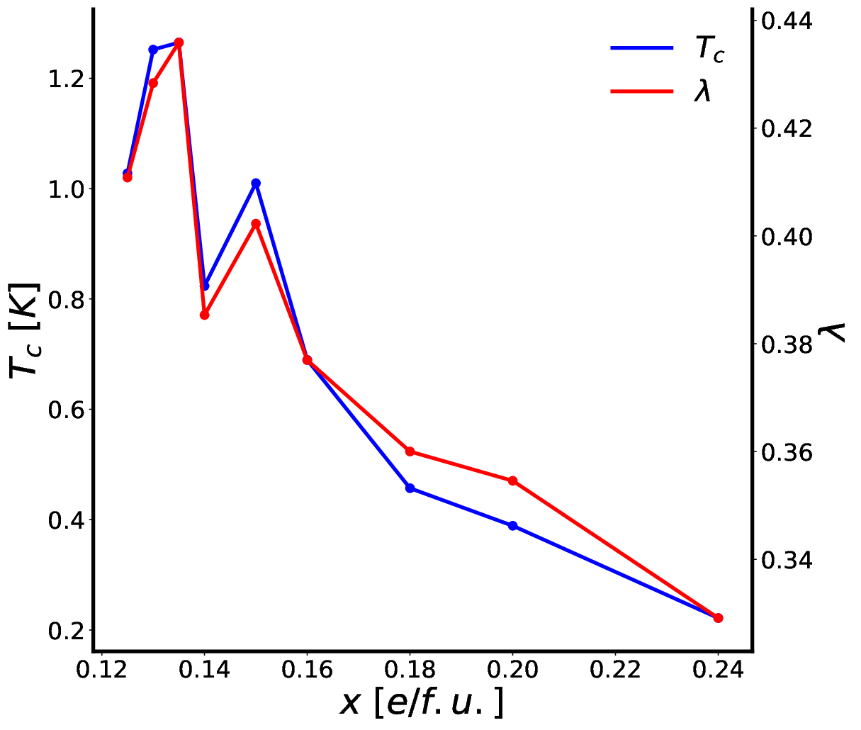
We begin by calculating the superconducting $T_{c}$ for the $\alpha_{1}$ phase, to see whether the measured decrease in $T_{c}$ with increasing doping is correctly captured within BCS theory. The $\alpha_{1}$ structure is stable for calculated electron concentrations larger than $x\approx 0.125$ (for lower concentrations, it has an unstable $Z_{3}^{+}$ mode, indicating the transition to the lower-energy $\alpha_{2}$ structure), which is therefore the lowest doping concentration that we consider. Our calculated electron bands, phonon bands, phonon linewidths, phonon density of states and Eliashberg spectral function $\alpha^{2}F$ for $x=0.125$ are shown in Fig. 8, where the soft $Z_{3}^{+}$ mode is the lowest frequency $Z$ mode in the phonon bands close to zero frequency. Interestingly, while there is some electron-phonon coupling at low frequency, it is considerably stronger at higher frequencies, with the highest values of $\alpha^{2}F$ occuring at around 600 - 800 cm^-1. This suggests that, at least in the BCS picture, the soft mode is not the most relevant in determining the superconducting $T_{c}$. The subsequent changes in the phonon bands and $\alpha^{2}F$ upon increase of $x$ are presented in Fig. 9. We see that, as expected, the $Z_{3}^{+}$ soft mode hardens with increasing doping, leading to a reduction of $\alpha^{2}F$ at low frequency with increasing doping. Interestingly, the high energy phonons shift to lower frequencies as doping is increased, with corresponding shifts of the peaks in $\alpha^{2}F$ to lower frequency. Finally, the calculated superconducting critical temperature, $T_{c}$, and density of states at the Fermi level, $n(E_{F})$, are shown in Fig. 10 as a function of doping concentration, $x$ ¹¹ 1 Note that we excluded the imaginary frequencies around $M$ ($q=[1/2,1/2,0]$) in our calculation of $\alpha^{2}F$ in the integration in equation (26). We also checked the influence of the adjacent real values that are close to zero by excluding the real part of the branch within a window bounded by a maximum frequency of $50\text{\,}{\mathrm{cm}}^{-1}$ and a box around $M$ defined by $\Delta q=0.2$ in each direction. We found that including or excluding the phonons in this window causes only a small change in the calculated $\alpha^{2}F$ (see appendix Fig. 14) between the two cases.. The first points in Fig. 10 (at $x=0.125$) correspond to the band structures shown in Fig. 8.

Fig. 10 clearly illustrates that our BCS-theory calculations reproduce the experimental trend of decreasing $T_{c}$ with increasing doping, with the calculated maximum in $T_{c}$ at $x=0.125$ coinciding with the calculated $\alpha_{1}-\alpha_{2}$ transition, where the transition $Z_{3}^{+}$ mode starts to become imaginary. In addition, our calculated $T_{c}$’s are comparable to the reported values ($\lesssim$ $2\text{\,}\mathrm{K}$ in bulk samples), although we emphasize that their actual magnitudes should not be over-interpreted, since they are sensitive to the spreads in $\alpha^{2}F$ integration in equation (26) and the value of the screened Coulomb potential $\mu$ in the Allen-Dynes formula (6). The trend of a decreasing $T_{c}$, however, is robust to these parameters. Therefore we conclude from our calculations that conventional BCS theory captures the observed evolution of $T_{c}$ with doping in the $\alpha_{1}$ phase of WO₃.²² 2 We note that a recent paper Pellegrini et al. 2019 using ostensibly similar methods obtained an increase in $T_{c}$ with increasing doping. We have been unable to reproduce the results of their work or understand the origin of the difference with our calculations. Note that they do reproduce the experimental behavior when they dope by introducing point defects rather than with electrostatic doping.

Given the good agreement of our computational BCS theory results with experiments, we next analyze them to rationalize the behavior. In particular, the decreasing $T_{c}$ with $x$ was unexpected within a simple BCS picture, since the electron density of states at the Fermi level, $n(E_{F})$, has been reported from photoemission measurements to increase with increasing $x$ in tetragonal $\text{Na}{\vphantom{\text{X}}}_{\smash[t]{\text{x\/}}}\text{WO}{\vphantom{\text{X}}}_{\smash[t]{\text{3\hskip 0.90417pt--\hskip 0.90417ptx\/}}}$ Höchst et al. 1982; Egdell and Hill 1982. Since the BCS Cooper-pair binding energy scales as $\exp\left[-1/(n(E_{F})V_{ep})\right]$ ($V_{ep}$ is the inter-electronic attraction caused by the electron-phonon coupling), an increase in $n(E_{F})$ should in turn lead to an increase in $T_{c}$, provided that the electron-phonon coupling strength remains constant with electron density. Our calculations of $n(E_{F})$ (Fig. 10) in fact indicate that, within the $\alpha_{1}$ phase, $n(E_{F})$ (red line) at first decreases with increasing doping (as does $T_{c}$). Note that there is no inconsistency with Refs. Höchst et al. 1982 and  Egdell and Hill 1982, which provided measured $n(E_{F})$ values only above $x=0.25$. At higher dopings (above $x=0.18$) $n(E_{F})$ starts to increase, while $T_{c}$ continues to decrease. This lack of correlation between $T_{c}$ and $n(E_{F})$ points to a doping dependence of the electron-phonon matrix elements.

In Fig. 11 we show our calculated doping dependence of $T_{c}$ and total coupling strength, $\lambda$, as defined in equation (25). First we note that, over the whole range, the coupling strength, $\lambda$, has a substantial value, consistent with the measurable superconductivity. Second, as we expected, it is clear that the value of $\lambda$ decreases with increasing doping, explaining the corresponding decrease in $T_{c}$ according to the Allen-Dynes formula given in equation 6. In particular, the calculated $T_{c}$ tracks closely the calculated value of $\lambda$.

Finally, to understand the change in superconductivity across the $\alpha_{1}-\alpha_{2}$ transition, we performed a calculation of $T_{c}$ in the $\alpha_{2}$ phase where experimentally superconductivity has not been measured. We chose a value of $x=0.125$ for the $T_{c}$ calculation in the $\alpha_{2}$ phase, and adjusted the lattice constants as outlined in section III.5 for the $\alpha_{1}$ phase, so that the resulting system in the $\alpha_{2}$ phase was quite far from the $\alpha_{1}-\alpha_{2}$ transition. (The amplitude of the transition mode $Z_{3}^{+}$ was $0.51\text{\,}\mathrm{\SIUnitSymbolAngstrom}$, compared with the amplitude of $0.76\text{\,}\mathrm{\SIUnitSymbolAngstrom}$ in the undoped $\alpha_{2}$ phase). As expected, our calculated $T_{c}$ dropped sharply from the calculated $\alpha_{1}$ value, to $0.018\text{\,}\mathrm{K}$, consistent with a sharp drop in the calculated $\lambda$ value to 0.25. The bands and linewidths for the $\alpha_{2}$ case are shown in appendix Fig. 15.

While our calculations indicate that the superconducting behavior of WO₃ can be reproduced within standard BCS theory, this is of course not definitive evidence that WO₃ is a BCS superconductor. In this section we discuss two other models for superconductivity – based on soft modes and bipolarons respectively – that have been discussed in the literature.

We begin with a discussion of the importance of the soft mode, whose strong change in frequency with doping was originally proposed to account for the apparently paradoxical behaviour of $T_{c}$ upon doping Shanks 1974, in spite of its absence in inelastic neutron scattering experiments Ngai and Silberglitt 1976; Ngai and Reinecke 1978. As mentioned above, our calculated phonon linewidths and doping dependence of $\alpha^{2}F$ point to a small, if any, role of the soft mode at the BCS level; here we quantify its contribution. In Fig. 12, we plot the calculated $T_{c}$ as a function of the maximum frequency of the phonons included in the calculation, for a range of doping values within the $\alpha_{1}$ phase. We see that the modes below $200\text{\,}{\mathrm{cm}}^{-1}$, which include the soft mode, contribute negligibly to $T_{c}$. As noted above, the modes above around $600\text{\,}{\mathrm{cm}}^{-1}$, which had the largest phonon bandwidth and the strongest frequency shifts on doping, contribute most to $T_{c}$ at every doping concentration.³³ 3 We note that again our findings are in contrast to those of Ref.  Pellegrini et al. 2019, who report that 60 % of the electron-phonon coupling comes from the lowest quarter of the spectrum. While our calculations were performed for tetragonal structures, we note that Brusetti et al. have attributed the increase in $T_{c}$ with decreasing $x$ in hexagonal $\text{Rb}{\vphantom{\text{X}}}_{\smash[t]{\text{x\/}}}\text{WO}{\vphantom{\text{X}}}_{\smash[t]{\text{3\hskip 0.90417pt--\hskip 0.90417ptx\/}}}$ to changes in electron-phonon coupling for phonons with a frequency of more than $240\text{\,}{\mathrm{cm}}^{-1}$ Brusetti et al. 2007.

Before leaving the topic of soft-mode superconductivity, we point out that the superconductivity in WO₃ is somewhat reminiscent of that in SrTiO₃, for which a model of superconductivity mediated by fluctuations associated with the ferroelectric quantum critical point has been proposed Edge et al. 2015. The quantum criticality model had considerable success in reproducing the measured behavior, as well as in making rather bold predictions about strain and isotope effects that were subsequently verified experimentally Stucky et al. 2016; Dunnett et al. 2018; Herrera et al. 2019; Schumann et al. 2020. An important difference is that SrTiO₃ has a superconducting dome as a function of doping, whereas in WO₃ an analogous picture would have the left side of the dome cut off due to the absence of superconductivity in the $\alpha_{2}$ phase. If this mechanism is relevant in WO₃, a large and anomalous oxygen isotope effect on $T_{c}$ should be observed.

Second, we note that electronic carriers in doped WO₃ have been shown, using optical absorption, conductivity and electron spin-resonance data, to form both polarons – in some cases in combination with free carriers Salje et al. 1979; Salje and Güttler 1984; Ruscher et al. 1988 – and bipolarons Schirmer and Salje 1980a; Schirmer and Salje 1980b. While it was speculated that bipolarons could be responsible for the high temperature surface superconductivity in H_xWO₃ Reich and Tsabba 1999, their role in mediating superconductivity in tungsten-based oxides was subsequently largely neglected until a recent measurement of sheet superconductivity in the shear planes of the $\text{WO}{\vphantom{\text{X}}}_{\smash[t]{\text{2.90}}}$ Magneli phase Shengelaya et al. 2020. The remarkably high reported $T_{c}$ of $80\text{\,}\mathrm{K}$ in this system was attributed to W⁵⁺-W⁵⁺ bipolarons, which were identified using electron paramagnetic resonance. A recent density functional study of self-trapped polarons in $\text{WO}{\vphantom{\text{X}}}_{\smash[t]{\text{3}}}$ succeeded in capturing a polaronic state, with substantial lattice distortions, in the simulations Bousquet et al. 2020, although the polaron was at higher energy than the delocalized electron. The role of electron localization and its coupling to the lattice is clearly an important area for future study Salje 2020.

To link our bulk $\text{WO}{\vphantom{\text{X}}}_{\smash[t]{\text{3}}}$ results to the sheet superconductivity reported at the $\text{WO}{\vphantom{\text{X}}}_{\smash[t]{\text{3}}}$ $\beta$ domain walls Aird et al. 1998; Aird and Salje 1998, we revisit the $\beta$ domain walls that we obtained from Landau-Ginzburg theory and our density functional calculations. We can make three main inferences. First, from both studies we see that it is lower energy for electronic charge to be at the domain than in the surrounding $\beta$ bulk structure leading to local charge accumulation at the walls. Second, this local increase in charge induces a local transition to the tetragonal bulk $\alpha_{1}$ phase in the domain walls. And third, the additional charge, combined with the presence of the $\alpha_{1}$ phase, leads to strong enough electron-phonon coupling to enable superconductivity in the domain walls.

Many of the samples in which domain wall superconductivity was measured showed a stripe pattern of parallel ferroelastic domain walls of only one type (see for example Ref. Aird and Salje 1998). Since similar samples were characterized in detail and shown to consist of $\beta$ domain walls Locherer et al. 1998, it is likely that the superconducting samples contained only $\beta$ domain walls. Whether $\gamma$ domain walls are also superconducting, and if so by what mechanism, is an interesting open question for future study.

References

- Granqvist (2000) C. Granqvist, Sol. Energy Mater. Sol. Cells 60, 201 (2000).
- Zheng et al. (2011) H. Zheng, J. Z. Ou, N. S. Strano, R. B. Kaner, A. Mitchell, and K. Kalantar-zadeh, Adv. Funct. Mater. 21, 2175 (2011).
- Santato et al. (2001) C. Santato, M. Odziemkowski, M. Ulmann, and J. Augustynski, J. Am. Chem. Soc. 123, 10639 (2001).
- Hagenmuller (1973) P. Hagenmuller, in Non-Stoichiometric Compounds (Pergamon, 1973) pp. 541 – 605.
- Raub et al. (1964) C. J. Raub, A. R. Sweedler, M. A. Jensen, S. Broadston, and B. T. Matthias, Phys. Rev. Lett. 13, 746 (1964).
- Sweedler et al. (1965a) A. Sweedler, C. Raub, and B. Matthias, Phys. Lett. 15, 108 (1965a).
- Sweedler et al. (1965b) A. Sweedler, J. Hulm, B. Matthias, and T. Geballe, Phys. Lett. 19, 82 (1965b).
- Hubble et al. (1971) F. Hubble, J. M. Gulick, and W. Moulton, J. Phys. Chem. Solids 32, 2345 (1971).
- Shanks (1974) H. R. Shanks, Solid State Commun. 15, 753 (1974).
- Skokan et al. (1979) M. R. Skokan, W. G. Moulton, and R. C. Morris, Phys. Rev. B 20, 3670 (1979).
- Cadwell et al. (1981) L. H. Cadwell, R. C. Morris, and W. G. Moulton, Phys. Rev. B 23, 2219 (1981).
- Garif’yanov et al. (1996) N. N. Garif’yanov, S. Y. Khlebnikov, I. S. Khlebnikov, and I. A. Garifullin, Czech. J. Phys. 46, 855 (1996).
- Salje et al. (1997) E. K. H. Salje, S. Rehmann, F. Pobell, D. Morris, K. S. Knight, T. Herrmannsdörfer, and M. T. Dove, J. Phys. Condens 9, 6563 (1997).
- Brusetti et al. (2002) R. Brusetti, P. Haen, and J. Marcus, Phys. Rev. B 65, 144528 (2002).
- Reich et al. (2009) S. Reich, G. Leitus, R. Popovitz-Biro, A. Goldbourt, and S. Vega, J. Supercond. Nov. Magn. 22, 343 (2009).
- Bocarsly et al. (2013) J. D. Bocarsly, D. Hirai, M. N. Ali, and R. J. Cava, EPL 103, 17001 (2013).
- Haldolaarachchige et al. (2014a) N. Haldolaarachchige, Q. Gibson, J. Krizan, and R. J. Cava, Phys. Rev. B 89, 104520 (2014a).
- Haldolaarachchige et al. (2014b) N. Haldolaarachchige, Q. Gibson, J. Krizan, and R. J. Cava, Phys. Rev. B 89, 104520 (2014b).
- Pellegrini et al. (2019) C. Pellegrini, H. Glawe, and A. Sanna, Phys. Rev. Materials 3, 064804 (2019).
- Reich and Tsabba (1999) S. Reich and Y. Tsabba, Eur. Phys. J. B 9, 1 (1999).
- Aird et al. (1998) A. Aird, M. C. Domeneghetti, F. Mazzi, V. Tazzoli, and E. K. H. Salje, J. Phys. Condens 10, L569 (1998).
- Aird and Salje (1998) A. Aird and E. K. H. Salje, J. Phys. Condens 10, L377 (1998).
- Aird and Salje (2000) A. Aird and E. K. H. Salje, Eur. Phys. J. B 15, 205 (2000).
- Locherer et al. (1998) K. Locherer, J. Chrosch, and E. K. H. Salje, Phase Transit. 67, 51 (1998).
- Salje and Lee (2004) E. K. H. Salje and W. T. Lee, Nat. Mater. 3, 425 (2004).
- Kim et al. (2010) Y. Kim, M. Alexe, and E. K. H. Salje, Appl. Phys. Lett. 96, 032904 (2010).
- Vogt et al. (1999) T. Vogt, P. M. Woodward, and B. A. Hunter, J. Solid State Chem. 144, 209 (1999).
- Crichton et al. (2003) W. A. Crichton, P. Bouvier, and A. Grzechnik, Mater. Res. Bull. 38, 289 (2003).
- Locherer et al. (1999a) K. R. Locherer, I. P. Swainson, and E. K. H. Salje, J. Phys. Condens. Matter 11, 6737 (1999a).
- Howard et al. (2001) C. J. Howard, V. Luca, and K. S. Knight, J. Phys. Condens. Matter 14, 377 (2001).
- Yun et al. (2015) S. Yun, C.-S. Woo, G.-Y. Kim, P. Sharma, J. H. Lee, K. Chu, J. H. Song, S.-Y. Chung, J. Seidel, S.-Y. Choi, and C.-H. Yang, Appl. Phys. Lett. 107, 252904 (2015).
- Salje (1991) E. K. H. Salje, in Phase Transitions in Ferroelastic and Co-elastic Crystals (Cambridge University Press, 1991) pp. 13–14.
- Aizu (1970) K. Aizu, J. Phys. Soc. Japan 28, 706 (1970).
- Sapriel (1975) J. Sapriel, Phys. Rev. B 12, 5128 (1975).
- Hatch and Stokes (2003) D. M. Hatch and H. T. Stokes, J. Appl. Crystallogr. 36, 951 (2003).
- Stokes et al. (2019) H. T. Stokes, D. M. Hatch, , and B. J. Campbell, “Isotropy software suite,” https://iso.byu.edu/iso/isotropy.php (2019).
- Walkingshaw et al. (2004) A. D. Walkingshaw, N. A. Spaldin, and E. Artacho, Phys. Rev. B 70, 165110 (2004).
- Wang et al. (2017) W. Wang, A. Janotti, and C. G. Van de Walle, J. Chem. Phys. 146, 214504 (2017).
- Hamdi et al. (2016) H. Hamdi, E. K. H. Salje, P. Ghosez, and E. Bousquet, Phys. Rev. B 94, 245124 (2016).
- García-Fernández et al. (2012) P. García-Fernández, S. Ghosh, N. J. English, and J. A. Aramburu, Phys. Rev. B 86, 144107 (2012).
- Krüger et al. (2012) P. Krüger, I. Koutiri, and S. Bourgeois, Phys. Rev. B 86, 224102 (2012).
- Wijs et al. (1999) G. A. d. Wijs, P. K. d. Boer, R. A. d. Groot, and G. Kresse, Phys. Rev. B 59, 2684 (1999).
- Huda et al. (2008) M. N. Huda, Y. Yan, C.-Y. Moon, S.-H. Wei, and M. M. Al-Jassim, Phys. Rev. B 77, 195102 (2008).
- Valdés and Kroes (2009) A. Valdés and G.-J. Kroes, J. Chem. Phys. 130, 114701 (2009).
- Wang et al. (2011) F. Wang, C. Di Valentin, and G. Pacchioni, J. Phys. Chem. C 115, 8345 (2011).
- Lambert-Mauriat et al. (2012) C. Lambert-Mauriat, V. Oison, L. Saadi, and K. Aguir, Surf. Sci. 606, 40 (2012).
- Ping et al. (2013) Y. Ping, D. Rocca, and G. Galli, Phys. Rev. B 87, 165203 (2013).
- Le et al. (2014) H. M. Le, N. H. Vu, and B.-T. Phan, Comput. Mater. Sci. 90, 171 (2014).
- Ping and Galli (2014) Y. Ping and G. Galli, J. Phys. Chem. C 118, 6019 (2014).
- Saadi et al. (2014) L. Saadi, C. Lambert-Mauriat, V. Oison, H. Ouali, and R. Hayn, Appl. Surf. Sci. 293, 76 (2014).
- Alvarez-Quiceno et al. (2015) J. C. Alvarez-Quiceno, G. M. Dalpian, and J. M. Osorio-Guillén, Phys. Status Solidi B 252, 2290 (2015).
- Gerosa et al. (2015) M. Gerosa, C. E. Bottani, L. Caramella, G. Onida, C. Di Valentin, and G. Pacchioni, Phys. Rev. B 91, 155201 (2015).
- Mehmood et al. (2016) F. Mehmood, R. Pachter, N. R. Murphy, W. E. Johnson, and C. V. Ramana, J. Appl. Phys. 120, 233105 (2016).
- Giannozzi et al. (2009) P. Giannozzi, S. Baroni, N. Bonini, M. Calandra, R. Car, C. Cavazzoni, D. Ceresoli, G. L. Chiarotti, M. Cococcioni, I. Dabo, A. D. Corso, S. de Gironcoli, S. Fabris, G. Fratesi, R. Gebauer, U. Gerstmann, C. Gougoussis, A. Kokalj, M. Lazzeri, L. Martin-Samos, N. Marzari, F. Mauri, R. Mazzarello, S. Paolini, A. Pasquarello, L. Paulatto, C. Sbraccia, S. Scandolo, G. Sclauzero, A. P. Seitsonen, A. Smogunov, P. Umari, and R. M. Wentzcovitch, J. Phys. Condens. Matter 21, 395502 (2009).
- Giannozzi et al. (2017) P. Giannozzi, O. Andreussi, T. Brumme, O. Bunau, M. B. Nardelli, M. Calandra, R. Car, C. Cavazzoni, D. Ceresoli, M. Cococcioni, N. Colonna, I. Carnimeo, A. D. Corso, S. de Gironcoli, P. Delugas, R. A. DiStasio, A. Ferretti, A. Floris, G. Fratesi, G. Fugallo, R. Gebauer, U. Gerstmann, F. Giustino, T. Gorni, J. Jia, M. Kawamura, H.-Y. Ko, A. Kokalj, E. Küçükbenli, M. Lazzeri, M. Marsili, N. Marzari, F. Mauri, N. L. Nguyen, H.-V. Nguyen, A. O. de-la Roza, L. Paulatto, S. Poncé, D. Rocca, R. Sabatini, B. Santra, M. Schlipf, A. P. Seitsonen, A. Smogunov, I. Timrov, T. Thonhauser, P. Umari, N. Vast, X. Wu, and S. Baroni, J. Phys. Condens. Matter 29, 465901 (2017).
- Hamann (2013) D. R. Hamann, Phys. Rev. B 88, 085117 (2013).
- Hamann (2019) D. R. Hamann, “Mat-sim research,” http://www.mat-simresearch.com (2019).
- van Setten et al. (2018) M. van Setten, M. Giantomassi, E. Bousquet, M. Verstraete, D. Hamann, X. Gonze, and G.-M. Rignanese, Comput. Phys. Commun. 226, 39 (2018).
- Pse (2019) “Pseudodojo github repository,” http://www.pseudo-dojo.org (2019).
- Kresse and Furthmüller (1996a) G. Kresse and J. Furthmüller, Comput. Mater. Sci 6, 15 (1996a).
- Kresse and Furthmüller (1996b) G. Kresse and J. Furthmüller, Phys. Rev. B 54, 11169 (1996b).
- Hacene et al. (2012) M. Hacene, A. Anciaux-Sedrakian, X. Rozanska, D. Klahr, T. Guignon, and P. Fleurat-Lessard, J. Comput. Chem. 33, 2581 (2012).
- Hutchinson and Widom (2012) M. Hutchinson and M. Widom, Comput. Phys. Commun. 183, 1422 (2012).
- Kresse and Hafner (1994) G. Kresse and J. Hafner, J. Phys. Condens. Matter 6, 8245 (1994).
- Kresse and Joubert (1999) G. Kresse and D. Joubert, Phys. Rev. B 59, 1758 (1999).
- Campbell et al. (2006) B. J. Campbell, H. T. Stokes, D. E. Tanner, and D. M. Hatch, J. Appl. Crystallogr. 39, 607 (2006).
- Giustino et al. (2007) F. Giustino, M. L. Cohen, and S. G. Louie, Phys. Rev. B 76, 165108 (2007).
- Ponce et al. (2016) S. Ponce, E. Margine, C. Verdi, and F. Giustino, Comput. Phys. Commun. 209, 116 (2016).
- Mostofi et al. (2014) A. A. Mostofi, J. R. Yates, G. Pizzi, Y.-S. Lee, I. Souza, D. Vanderbilt, and N. Marzari, Comput. Phys. Commun. 185, 2309 (2014).
- Bruneval et al. (2015) F. Bruneval, C. Varvenne, J.-P. Crocombette, and E. Clouet, Phys. Rev. B 91, 024107 (2015).
- Locherer et al. (1999b) K. R. Locherer, I. P. Swainson, and E. K. H. Salje, J. Phys. Condens. Matter 11, 4143 (1999b).
- Salje (2020) E. K. H. Salje, Condens. Matter 5 (2020), 10.3390/condmat5020032.
- Triantafyllou et al. (1997) S. Triantafyllou, P. Christidis, and C. Lioutas, J. Solid State Chem. 133, 479 (1997).
- Ngai and Silberglitt (1976) K. L. Ngai and R. Silberglitt, Phys. Rev. B 13, 1032 (1976).
- Bardeen et al. (1957) J. Bardeen, L. N. Cooper, and J. R. Schrieffer, Phys. Rev. 108, 1175 (1957).
- Stanley et al. (1979) R. K. Stanley, R. C. Morris, and W. G. Moulton, Phys. Rev. B 20, 1903 (1979).
- Reich et al. (2000) S. Reich, G. Leitus, Y. Tssaba, Y. Levi, A. Sharoni, and O. Millo, J. Supercond. Nov. Magn. 13, 855 (2000).
- Ngai and Reinecke (1978) K. L. Ngai and T. L. Reinecke, J. Phys. F. Met. Phys. 8, 151 (1978).
- Brusetti et al. (2007) R. Brusetti, P. Bordet, J. Bossy, H. Schober, and S. Eibl, Phys. Rev. B 76, 174511 (2007).
- Baroni et al. (2001) S. Baroni, S. de Gironcoli, A. Dal Corso, and P. Giannozzi, Rev. Mod. Phys. 73, 515 (2001).
- Allen and Dynes (1975) P. B. Allen and R. C. Dynes, Phys. Rev. B 12, 905 (1975).
- (82) Note that we excluded the imaginary frequencies around () in our calculation of in the integration in equation (26). We also checked the influence of the adjacent real values that are close to zero by excluding the real part of the branch within a window bounded by a maximum frequency of and a box around defined by in each direction. We found that including or excluding the phonons in this window causes only a small change in the calculated (see appendix Fig. 14) between the two cases.
- (83) We note that a recent paper Pellegrini et al. 2019 using ostensibly similar methods obtained an increase in with increasing doping. We have been unable to reproduce the results of their work or understand the origin of the difference with our calculations. Note that they do reproduce the experimental behavior when they dope by introducing point defects rather than with electrostatic doping.
- Höchst et al. (1982) H. Höchst, R. D. Bringans, and H. R. Shanks, Phys. Rev. B 26, 1702 (1982).
- Egdell and Hill (1982) R. Egdell and M. Hill, Chem. Phys. Lett. 85, 140 (1982).
- (86) We note that again our findings are in contrast to those of Ref. \rev@citealpnumPellegrini2019, who report that 60 % of the electron-phonon coupling comes from the lowest quarter of the spectrum.
- Edge et al. (2015) J. M. Edge, Y. Kedem, U. Aschauer, N. A. Spaldin, and A. V. Balatsky, Phys. Rev. Lett. 115, 247002 (2015).
- Stucky et al. (2016) A. Stucky, G. W. Scheerer, Z. Ren, D. Jaccard, J.-M. Poumirol, C. Barreteau, E. Giannini, and D. van der Marel, Sci. Rep. 6, 37582 (2016).
- Dunnett et al. (2018) K. Dunnett, A. Narayan, N. A. Spaldin, and A. V. Balatsky, Physical Review B 97, 144506 (2018).
- Herrera et al. (2019) C. Herrera, J. Cerbin, A. Jayakody, K. Dunnett, A. V. Balatsky, and I. Sochnikov, Phys. Rev. Materials 3, 124801 (2019).
- Schumann et al. (2020) T. Schumann, L. Galletti, H. Jeong, K. Ahadi, W. M. Strickland, S. Salmani-Rezaie, and S. Stemmer, Phys. Rev. B 101, 100503 (2020).
- Salje et al. (1979) E. Salje, A. Carley, and M. Roberts, J. Solid State Chem. 29, 237 (1979).
- Salje and Güttler (1984) E. Salje and B. Güttler, Philos. Mag. B 50, 607 (1984).
- Ruscher et al. (1988) C. Ruscher, E. Salje, and A. Hussain, J. Phys. C: Solid State Phys. 21, 4465 (1988).
- Schirmer and Salje (1980a) O. Schirmer and E. Salje, Solid State Commun. 33, 333 (1980a).
- Schirmer and Salje (1980b) O. F. Schirmer and E. Salje, J. Phys. C 13, L1067 (1980b).
- Shengelaya et al. (2020) A. Shengelaya, K. Conder, and K. A. Müller, J. Supercond. Nov. Magn. 33, 301 (2020).
- Bousquet et al. (2020) E. Bousquet, H. Hamdi, P. Aguado-Puente, E. K. H. Salje, E. Artacho, and P. Ghosez, Phys. Rev. Research 2, 012052 (2020).
- Artyukhin et al. (2014) S. Artyukhin, K. T. Delaney, N. A. Spaldin, and M. Mostovoy, Nat. Mater. 13, 42 (2014).
- Migdal (1958) A. Migdal, Sov. Phys. JETP 34, 996 (1958).
- McMillan (1968) W. L. McMillan, Phys. Rev. 167, 331 (1968).
- Noffsinger et al. (2010) J. Noffsinger, F. Giustino, B. D. Malone, C.-H. Park, S. G. Louie, and M. L. Cohen, Comput. Phys. Commun. 181, 2140 (2010).