Engineering spatial coherence in lattices of polariton condensates

In our study of synchronisation in networks of coupled polariton condensates we are interested in the correlations between pairs of condensates which are described by their mutual coherence function

where the brackets denote ensemble averaging and $\psi_{i}(t)$ is the complex-valued amplitude of the $i$th condensate node. The expectation value of the condensate’s particle number (occupation) is given by the diagonal elements $\Gamma_{ii}(t)$, and the presence of non-zero off-diagonal elements $|\Gamma_{ij}(t)|>0$ for $i\neq j$ indicates long-range order in the coupled condensate network. For nonstationary systems (such as for polariton condensates generated under pulsed excitation) the coherence function $\Gamma_{ij}(t)$ depends on time $t$. We note that pulsed excitation ($\approx 150\;\mathrm{fs}$ pulse width) of ballistically coupled condensate nodes leads to polariton photoluminescence with typical emission signal full-width-at-half-maximum (FWHM) of $18\;\mathrm{ps}$ (see Appendix G). A normalised form of the mutual coherence function is given by the complex coherence factor

where for a fully coherent pair of condensates $|\mu_{ij}|$ = 1. Considering measurements with time integration over many pulses we define the integrated complex coherence factor

as an averaged measure for the mutual coherence properties of condensates in polariton networks. Throughout this manuscript time-integrated variables are marked with the tilde diacritic. For stationary ergodic systems (such as polariton condensates under constant pumping) the complex coherence factor $\mu_{ij}(t)$ does not depend on time and time-integrated measurements of correlations fully determine the coherence properties, i.e. $\mu_{ij}(t)=\tilde{\mu}_{ij}$. In case of pulsed excitation of polariton condensates the modulus of the time-integrated factor $|\tilde{\mu}_{ij}|$ represents a lower bound for the maximum value of the complex coherence factor $|\mu_{ij}(t)|$. We note that the argument of the integrated complex coherence factor represents the average condensate node phase difference $\tilde{\theta}_{ij}=\arg(\tilde{\mu}_{ij})$ and the integrated particle number $\int\Gamma_{ii}(t)\mathrm{d}t$ of each condensate node is proportional to its measurable average emission intensity $\tilde{I}_{i}$.

In this manuscript we present networks of ballistically coupled polariton condensates for which the pumping geometry has been adjusted using a reflective SLM (see Fig. 1) such as to equalise the emission power of each condensate node at condensation threshold. The algorithm used to calculate the holograms which are applied to the SLM is a modified version of the Gerchberg-Saxton (GS) algorithm Gerchberg and Saxton 1972 and takes into account feedback from the recorded PL. This iterative algorithm is similar to the schemes presented in Refs. [Nogrette et al. 2014,Tamura et al. 2016] applied to trapping of cold atoms. In our case the recorded PL of the condensates is not directly proportional to the pump power of each node but depends on the coupling-topology of the network, i.e. ballistic coupling between spatially separated condensate nodes affects the gain of each condensate.

The algorithm is schematically illustrated in Fig. 7(a) and begins with the initialisation of a 2D complex field of amplitude $A^{(0)}(\mathbf{r})$ and phase $\phi^{(0)}(x,y)$ representing the amplitude of the pump laser and the phase hologram in pixel coordinates of the SLM, respectively. As an initial guess we assume a constant phase pattern $\phi^{(0)}=0$ and a Gaussian field amplitude, whose width matches the pump laser width. In each iteration step $n$ propagation of the complex field $A^{(0)}e^{i\phi^{(n)}(\mathbf{r})}$ from the SLM plane to the focal plane is computed by a fast Fourier transform (FFT) yielding a complex-valued target field with amplitude $\tilde{A}^{(n)}(\mathbf{r})$ and phase $\phi_{\mathrm{GS}}^{(n)}(\mathbf{r})$. We add the output phase pattern $\phi_{\mathrm{GS}}^{(n)}$ with a device dependent correction term $\phi_{c}$, which can also take into account optical aberrations in the experimental setup, and a blazed grating $\phi_{g}$ to offset the modulated laser beam from its unmodulated reflected part. The sum of these terms modulo the $2\pi$ bitlevel is applied to the SLM and defines the pump laser geometry. In a next step we record the near-field photoluminescence of the polariton system excited by the current pump laser geometry and extract the emission power $I_{\mathrm{C}}^{(n)}$ of each condensate by integrating the recorded signal within the FWHM ($\approx 2\;\mathrm{\upmu m}$) of each node. We update the target power $I_{\mathrm{T}}^{\mathrm{(n+1)}}$ for the next iteration step of the algorithm for each condensate node utilising the non-linear function

where $\epsilon$ is an adjustable feedback parameter and $\langle I^{(n)}_{C}\rangle$ denotes the mean of the measured condensate node emission distribution. The non-linear mapping given by Eq. (10) lowers (raises) the target pump power $I^{(n+1)}_{T}$ of nodes with measured emission power $I^{(n)}_{C}$ larger (lower) than the mean value $\langle I^{(n)}_{C}\rangle$. The parameter $\epsilon$ controls the speed of the feedback loop but cannot be set too large to avoid destabilisation of the algorithm. For $\epsilon=0$ the algorithm represents the conventional form of the GS algorithm with no iterative adjustment of target spot intensities, i.e. $I^{(n+1)}_{T}=I^{(n)}_{T}$. Next, a complex-valued target field with amplitude $\sqrt{I_{\mathrm{T}}}(\mathbf{r})$ and phase $\phi_{\mathrm{GS}}^{(n)}(\mathbf{r})$ is constructed. Hereby, the field amplitude $\sqrt{I_{\mathrm{T}}}(\mathbf{r})$ consists of the superposition of Gaussian spots representing the position of each condensate node. The amplitude of each Gaussian peak is given by the square root of the updated spot power, i.e. $\sqrt{I_{\mathrm{T}}^{\mathrm{(n+1)}}}$ and the width is related to the width of the Gaussian profile of the pump laser by means of a Fourier transform. Back-propagation of this complex field to the SLM plane is computed by an inverse fast Fourier transform (IFFT) yielding a phase pattern $\phi^{(n+1)}$ which replaces the initial phase pattern for the next iteration step, i.e. $\phi^{(n+1)}\rightarrow\phi^{(n)}$. The amplitude field at the SLM plane is kept constant as the initial field $A^{(0)}$ for each iteration step. We quit execution of the algorithm once the measured spot power distribution $I_{\mathrm{C}}^{(n)}$ shows a spread which is smaller than a certain threshold level (usually $1\%\;\mathrm{(RSD)}$ reached within $<100\;$iterations).

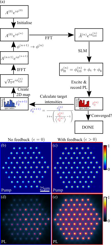
We find good results for stabilising the intensity distribution in ballistically coupled polariton networks ($\mathrm{RMS}\leq 1\%$) pumped at condensation threshold $P\gtrsim P_{\mathrm{thr}}$ by choosing $\epsilon$ to be in the range $10^{-2}-10^{-1}$. Stabilisation at larger pump powers $P\gg P_{\mathrm{thr}}$ is impeded using the presented technique - which operates at a typical rate of $60\;\mathrm{Hz}$ - because of stronger nonlinear effects resulting in unstable regimes Wouters and Carusotto 2007; Bobrovska et al. 2014; Baboux et al. 2018 and/or excitement of polaritons to higher energy states Wertz et al. 2010, with subsequent nonstationary condensate dynamics on a picosecond timescale.

In Fig. 7(b) we show the recorded laser (pump) profile for a triangular lattice of 61 nodes (lattice constant $a=14.9\;\mathrm{\upmu m}$) using a phase hologram computed with the conventional GS algorithm ($\epsilon=0;100\;\mathrm{iterations}$). Although the target image is a laser pattern with homogeneous spot intensities, due to limited accuracy of the algorithm as well as unavoidable optical aberrations due to misalignment and device imperfections, the resultant experimentally obtained pump spot intensity distribution deviates from the homogeneous target. We measure a spread of $\approx 17\%$ (RSD) for the distribution of pump spot powers. Using the same pump profile to excite a triangular lattice of polariton condensates at condensation threshold ($P\approx P_{\mathrm{thr}}$) we record the near-field PL as shown in Fig. 7(d) and find an increased spread of condensate node densities of $\approx 37\%\;\mathrm{(RSD)}$. While sample disorder can have an impact on the spatially dependent condensation threshold pump power and emission intensity for each condensate node, the main reason for the increased spread in the condensate emission power distribution is due to the system’s nonlinear input-output-power characteristics and the finite size of the system. Nodes that are positioned at the edge of the condensate network are coupled to fewer nearest-neighbours (NN) than nodes in the bulk. Since coherent coupling between ballistically expanding polariton condensates results in a reduced condensation threshold Cristofolini et al. 2013, nodes coupled to fewer NNs will typically have a higher threshold pump power than nodes with a greater number of NNs (see section B). As a result, condensate nodes in the bulk of the network generally have a larger occupation number (emission) than condensate nodes at the edges when pumped with the same excitation pump power Kalinin and Berloff 2018. This is a consequence of polariton waves radiating to the outside continuum and escaping the network which can be regarded as an effective flux-induced potential Ostrovskaya et al. 2013.
In Figs. 7(c,e) we show the recorded pump laser and corresponding near-field polariton emission profiles at threshold $P\approx P_{\mathrm{thr}}$ after applying the intensity stabilisation feedback loop and terminating it with spread in condensate node densities of $\approx 1\%\;\mathrm{(RSD)}$. Comparison of the density spread and the spatial coherence in both polariton lattices without ($\epsilon=0$) and with ($\epsilon>0$) is shown in Fig. 1.

The time-averaged far-field interference pattern $\tilde{I}(\mathbf{k})$ of a set of $N$ partially coherent, narrow-bandwidth and point-like light sources positioned in one plane can be written in the basis of spatial frequencies $\mathbf{k}$ as (see Appendix J)

For each pair $\{i,j\}$ of point sources $\mathbf{d}_{ij}$ denotes their in-plane spatial separation vector and $\tilde{\mu}_{ij}$ their respective integrated complex coherence factor. For an incoherent system ($\tilde{\mu}_{ij}=0$ for $i\neq j$) the resulting homogeneous far-field radiation pattern is the incoherent superposition of light sources with individual intensities $\tilde{I}_{i}$. However, for non-vanishing off-diagonal coherence elements ($|\tilde{\mu}_{ij}|>0$) the radiation pattern $\tilde{I}(\mathbf{k})$ described in Eq. (11) becomes inhomogeneous and is formed by the sum over discrete Fourier-components $\exp{(i\mathbf{k}\cdot\mathbf{d}_{ij})}$ weighted by the integrated complex coherence factor $\tilde{\mu}_{ij}$.

Hence, in analogy to beam interference measurements of coupled laser arrays Mahler et al. 2020, we can investigate the far-field emission of the coupled polariton condensate network to gain information about the system’s spatial coherence properties. To remove residual PL coming from polaritons outside the condensation (gain-)centres we spatially filter the emission of each condensation center and measure the interference of the masked condensate emission in the far field. As schematically illustrated in Fig. 8(a) we project the near-field PL onto a programmable aperture which allows to selectively mask the real space field $\Psi(\mathbf{r},t)\rightarrow A(\mathbf{r})\Psi(\mathbf{r},t)$ with amplitude function $A(\mathbf{r})\in(0,1)$. Subsequently we image the diffraction pattern (far field) onto a charge-coupled device (CCD) sensor. The programmable aperture consists of a digitally controllable reflective liquid-crystal SLM as described in reference Lousberg et al. 2006. With the use of an additional wave plate and linear polariser the apparatus transmits only circular polarised light which is chosen to be the same as the polarisation of the pump laser beam. By projecting the near-field PL of the polariton condensate lattice (Fig. 8(b)) onto an aperture that transmits only the central $\mathrm{FWHM}\approx 2\;\mathrm{\upmu m}$ of each condensation centre (Fig. 8(c)) we record the corresponding far-field emission (Fig. 8(d)) that consists of the interference of all condensate nodes. According to the Fraunhofer diffraction formula the measured far-field intensity distribution for a fully coherent wave is proportional to the squared modulus of the Fourier transform of the optical field at the aperture location, which is obtained from Eq. (11) for $|\tilde{\mu}_{ij}|=1$ for all pairs $\{i,j\}$. Indeed, the appearance of the reciprocal triangular lattice, shown in Fig. 8(d), indicates long-range coherence across the triangular lattice of polariton condensates.

Far field measurements shown in Fig. 8 give information about the global coherence properties of the coupled condensate network and are analogous to time-of-flight experiments used in cold atom systems Hadzibabic et al. 2006. However, precise information about the local complex coherence factor $\mu_{ij}$ can not be obtained. The programmable aperture in our experiment (see Fig. 8) overcomes this problem and allows for selective interference between any pair $\left\{i,j\right\}$ of condensates, such that the complex coherence factor $\mu_{ij}$ can be spatially reconstructed Lousberg et al. 2006; Lundeberg et al. 2007. In particular, the far-field interference of the emission of two spatially filtered condensate nodes $\psi_{i}(\mathbf{r},t)$ and $\psi_{j}(\mathbf{r},t)$ centred around their respective positions $\mathbf{r}_{i}$ and $\mathbf{r}_{j}$ yields the measurable intensity pattern $\tilde{I}_{i+j}(\mathbf{k})$ in $\mathbf{k}$-space as, Thompson and Wolf 1957

where we explicitly take into account non-homogeneous intensity distributions $\tilde{I}_{i,j}(\mathbf{k})$ due to the finite aperture sizes. In Fig. 9 we project the triangular lattice of 61 condensates (a) onto three different apertures filtering the emission of the central-most condensate (b), of one of its nearest-neighbours (c) and of both condensates simultaneously (d). The corresponding measured far-field diffraction patterns $\tilde{I}_{1}(\mathbf{k})$, $\tilde{I}_{2}(\mathbf{k})$ and $\tilde{I}_{1+2}(\mathbf{k})$ are shown in Figs. 9(e-g) respectively. We extract 1D intensity profiles $\tilde{I}(k_{\parallel})$ along the direction vector $\mathbf{k}_{\parallel}$, which is defined as co-parallel to $\mathbf{d}_{12}$ such that $\mathbf{k}_{\parallel}\cdot\mathbf{d}_{12}=k_{\parallel}|\mathbf{d}_{12}|$. Equation (12) can be rewritten as,

and is fitted to the experimentally extracted intensity profiles $\tilde{I}_{1}(k_{\parallel})$, $\tilde{I}_{2}(k_{\parallel})$ and $\tilde{I}_{1,2}(k_{\parallel})$ to yield $|\tilde{\mu}_{12}|$ and $\tilde{\theta}_{12}$ as shown in Fig. 9(h). By extracting $|\tilde{\mu}_{12}|$ for varying pump power we identify the threshold-like behaviour of coherence shown in Fig. 9(i) with vanishing coherence between the two nodes below threshold and a sharp increase at threshold. The observed decrease of coherence for larger pump powers $P>1.2P_{\mathrm{thr}}$ is attributed to effects involving dephasing due to increased particle interactions, reservoir induced noise, enhanced proliferation of topological defects, as well as to the emergence of multi-mode emission Ohadi et al. 2016 reducing the fringe visibility in time-integrated measurements.

Repeating the interference measurement for the central condensate node $1$ and each other condensate node $j$ we fully characterise the spatial coherence properties of the central condensate node within the triangular lattice (see Figs. 9(j,k) or Figs. 1(e,f)).

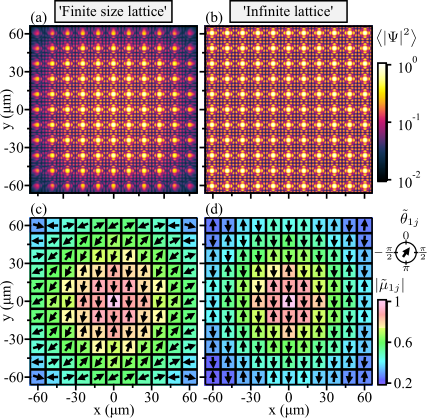
In experiment finite-size effects cannot be avoided whereas in theory they can by applying periodic boundary conditions. In Fig. 10 we investigate the difference of finite and periodic systems through simulation of Eq. (9). In agreement with experiment, and previous theoretical observations Kalinin and Berloff 2018, the pseudo-spin of $\tilde{\mu}_{ij}$ tilts as one approaches the edges of the finite (damped boundary condition) condensate lattice (see Fig. 10(c)). This effect is expected due to the non-zero flux of particles through the boundaries of the lattice resulting in a phase gradient differing from standing wave solutions of $\tilde{\theta}_{ij}=0,\pi$. When the system has periodic boundary conditions (see Fig. 10(d)) the pseudo-spin tilt vanishes and the lattice is characterised by a homogeneous standing wave solution (zero net-flux along $x$ and $y$ directions). The simulation in both cases uses a lattice constant of $a=12$ $\upmu$m and is performed on a $16a\times 16a$ grid but we only plot the innermost $11a\times 11a$ of the grid. Therefore, removing finite size effects results in a homogeneous power distribution among all condensate nodes and thus the phases-differences stay homogeneously $0$ or $\pi$.

We point out that by simulating a periodic system the coherence has dropped by a small amount. This can be understood from the fact that each pulse proliferates vortex solitons Neshev et al. 2004 which, in a finite system, can decay out through the boundary of the system (i.e., damped boundary conditions destroy such defects). In the absence of such a decay channel, these defect states can survive much longer in a periodic system leading to a drop in coherence.

In this section we describe the pump power dependence of the stabilised triangular lattice of 61 ballistically coupled polariton condensates with lattice constant $a=14.9\;\mathrm{\upmu m}$ shown in Figs. 1 and 2. For the case of pulsed excitation the pump power $P$ is a time-averaged value and a change of $P$ is equivalent to changing the peak amplitude of the sub-picosecond laser pulse. The recorded emission patterns for pump power $P=1.2P_{\mathrm{thr}}$ in near-field, far-field and energy resolved far-farfield along the symmetry axis $k_{x}=0$ are illustrated in Figs. 11(a,c,e). The pump power geometry was adjusted using the described iterative feedback algorithm to stabilise the emission power of all condensates at threshold such that the spread of measured condensate emission powers shows a minimum of $1\%$ (RSD) for $P=P_{\mathrm{thr}}$. In Fig. 11(b) we show the spread of condensate emission powers for varying total excitation pump power while keeping the relative pump power between different nodes constant. An increase of the spread above condensation threshold to about $20\%$ at $P=1.2P_{\mathrm{thr}}$ originates from the different number of coupled neighbouring sites between condensates in the centre and at the edge of the lattice structure leading to different additional gain from coherent coupling between condensate nodes.

In Fig. 11(d) we illustrate the pump power dependence of the total integrated PL demonstrating a threshold level with non-linear increase of PL intensity which we define as condensation threshold $P_{\mathrm{thr}}$. An increase in pump power from condensation threshold $P_{\mathrm{thr}}$ to the operational point $P=1.2P_{\mathrm{thr}}$ leads to a 9-fold increase of total PL power.

The spectrally resolved PL in reciprocal space along the symmetry axis $k_{x}=0$ in Fig. 11(e) demonstrates PL emission at one dominant mode with $\mathrm{FWHM}\approx 250\;\mathrm{\upmu eV}$. In agreement with the threshold-like behaviour of the integrated PL we can see a sharp narrowing of polariton linewidth at condensation threshold which is shown in Fig. 11(f) .

The time-resolved formation of coherence in polariton condensates under non-resonant pulsed excitation has been investigated for single- Nardin et al. 2009; Belykh et al. 2013 and two-condensate systems Christmann et al. 2014; Ohadi et al. 2016. In the latter case, however, a full description of the synchronisation process between two condensates in terms of their complex coherence factor has not been reported. Here, we explicitly measure the (time-resolved) complex coherence factor $\mu_{12}(t)$ of two ballistically coupled condensation centres. Pulsed excitation of two condensates with separation distance $d_{12}=8\;\mathrm{\upmu m}$ leads to the time-averaged near-field photoluminescence displayed in Fig. 12(a). The pump power $P\approx 1.2P_{\mathrm{thr}}$ is the same as for the distance-dependence shown in Fig. 3 in the main manuscript. One bright interference peak located in-between the two condensation centres at $x,y=0$ indicates synchronisation with vanishing phase-difference, i.e. $\tilde{\theta}_{12}=0$. To reveal the coherence properties between the two condensates we record their far-field interference by spatially filtering the emission of both condensation centres (red-dashed circles) as shown in Fig. 12(b). The modulus of the integrated coherence factor from this time-averaged interference pattern is extracted as $|\tilde{\mu}_{12}|=0.94$. By projecting the far-field pattern onto the entrance slit of a streak camera (time resolution $\Delta t\approx 2\;\mathrm{ps}$) we resolve the interference and emission of each individual condensate node in time as shown in Figs. 12(c-e). We extract the time-dynamics of the mutual complex degree of coherence $\mu_{12}(t)$ from the measured interference and reference signals and illustrate its phase $\theta_{12}(t)$ and modulus $|\mu_{12}(t)|$ in Figs. 12(f) and (g), respectively. The time-resolved occupation $\Gamma_{11}(t)+\Gamma_{22}(t)$ with $\Gamma_{ii}(t)=\langle|\psi_{i}(t)|^{2}\rangle$ of both condensates is shown in Fig. 12(h) and reveals pulsed polariton emission with temporal width $\approx 18\;\mathrm{ps}$ (FWHM) and peak signal at $50\;\mathrm{ps}$ after excitation with the pump laser. We find complete synchronisation with $\theta_{12}=0$ and a maximum degree of coherence $|\mu_{12}|=1$ appearing earlier than the peak PL signal at $t=41\;\mathrm{ps}$ still during the condensate growth time. The subsequent temporal decay of mutual coherence is slower than the decay of total condensate population with fitted $1/e$ decay times of $80\;\mathrm{ps}$ and $13\;\mathrm{ps}$, respectively.

We compare the results of mutual coherence between two ballistically expanding polariton condensates pumped under sub-picosecond excitation shown in Fig. 3 to the case of pumping using continuous wave (cw) monomode laser excitation. To prevent heating of the microcavity sample under cw excitation, the excitation laser is modulated by an acousto-optic modulator to generate square wave packets of $5\;\mathrm{\upmu s}$ duration at a frequency of $10\;\mathrm{kHz}$. In Figs. 13(a) and (b) we illustrate the recorded near-field and far-field photoluminescence of two condensate with separation distance $d=12\;\mathrm{\upmu m}$. The system is pumped at $P=1.6P_{\mathrm{thr}}$ with a threshold pump power $P_{\mathrm{thr}}\approx 10\;\mathrm{mW}$ per condensate node as shown in Fig. 13(c). We note that the near-field and far-field excitation pattern in (a) and (b) are different to the emission patterns shown in Fig. 3(a) and (b) under pulsed excitation despite a small difference in pump spot separation distance of less than $1\;\mathrm{\upmu m}$. In both cases the emission patterns indicate synchronisation in a state with $\pi$ phase-difference between the two condensate nodes. However, the outflow wavevector (or alternatively in-plane momentum) of polaritons under pulsed excitation is larger than under cw excitation leading to a smaller interference fringe periodicity in both real- and momentum-space.

The extracted decay of the complex coherence factor $\mu_{12}$ with increasing condensate separation distance under cw excitation is illustrated in Fig. 13(d). In the same plot we show the dependency of the integrated complex coherence factor $\tilde{\mu}_{12}$ on the separation distance $d_{12}$ of two condensates under pulsed excitation condition (as presented in Fig. 3). While both systems demonstrate similar coherence properties for condensate separation distances $d_{12}\leq 20\;\mathrm{\upmu m}$, the stationary system’s coherence $|\mu_{12}|$ is enhanced for distances larger than $20\;\mathrm{\upmu m}$ as compared to the nonstationary system under sub-picosecond pulsed excitaiton. A Gaussian fit (see Eq. 2) of the decay of coherence $|\mu_{12}(d_{12})|$ with increasing condensate spacing under cw excitation yields an effective coherence length $L_{C}=40\;\mathrm{\upmu m}$. We argue that the build-up of coherence $|\mu_{12}(t)|$ between the two ballistically coupled condensates under pulsed excitation (as described in Appendix G) is fast enough for small distances $d_{12}\leq 20\;\mathrm{\upmu m}$ as to synchronise and reach the same coherence $|\mu_{12}|$ as in steady-state operation. For larger distances, however, the increased time-of-flight of particles travelling in-between the two condensate nodes Töpfer et al. 2020 becomes noticeable and reduces the coherence factor $|\tilde{\mu}_{12}|$ of the nonstationary system with finite life-time.

Let us consider the continuous-wave excitation regime where $n_{c}(\mathbf{r})=P(\mathbf{r})$ is taken time-independent. We will also consider the ideal case of no stochasticity by setting $dW=0$. Assuming that the reservoir $n_{x}$ follows the dynamics of the condensate we can perform an adiabatic elimination of Eq. (9b) and keeping terms to the first order in $R$ in Eq. (9a) we have,

where $n_{s}=\Gamma_{R}/R$. Performing the standard Bogoliubov treatment where the condensate wavefunction $\Psi$ is expanded around a fixed point solution of Eq. (14) $\Psi_{0}$ with energy $\hbar\nu$ we write,

We wish to scrutinise the dispersion of elementary excitations (Lyapunov exponents) with complex energies $\lambda_{n}$. Substitution of Eq. (15) into (14) and keeping only terms linear in $u_{n,\mathbf{q}}$ and $v_{n,\mathbf{q}}$ we obtain a linearised set of equations of motion for the disturbances. We assume that the potential $V$ and condensate $\Psi_{0}$ are infinite and periodic such that $P(\mathbf{r})=P(\mathbf{r}+\mathbf{a})$ and $|\Psi_{0}(\mathbf{r})|^{2}=|\Psi_{0}(\mathbf{r}+\mathbf{a})|^{2}$, where $\mathbf{a}=n_{1}\mathbf{a}_{1}+n_{2}\mathbf{a}_{2}$ is the translational symmetry vector defined in the bases of primitive lattice vectors $\mathbf{a}_{1,2}$ for some integers $n_{1,2}$. We can then apply Bloch’s theorem where we write the disturbances wavefunction in the factorised form of crystal momentum $\mathbf{q}=(q_{x},q_{y})$ and Bloch states in the $n$th band $u_{n,\mathbf{q}}(\mathbf{r})=u_{n,\mathbf{q}}(\mathbf{r}+\mathbf{a})$ and $v_{n,\mathbf{q}}(\mathbf{r})=v_{n,\mathbf{q}}(\mathbf{r}+\mathbf{a})$.

By Fourier transforming periodic terms into the basis of reciprocal lattice vectors we can easily solve the energies $\lambda_{n}$ belonging to $u_{n,\mathbf{q}}$ and $v_{n,\mathbf{q}}$,

where $\mathcal{L}$ is our Bogoliubov (Lyapunov) matrix in the crystal momentum representation,

The solution $\Psi_{0}$ satisfying Eq. (14) can be obtained numerically using periodic boundary conditions. Plugging the obtained solution $\Psi_{0}$, which corresponds to observed condensate patterns in experiment, into the eigenvalue problem for $\mathbf{B}_{n,\mathbf{q}}$ we can finally diagonalise our system.

Let us assume the narrow bandwith optical field $\Psi(\mathbf{r},t)=\psi(\mathbf{r,t})\exp{(-i2\pi ct/\bar{\lambda})}$ with mean wavelength $\bar{\lambda}$ is being truncated by a thin aperture with transmittance function $P(\mathbf{r})$ in the plane $\mathcal{A}$ such that the field directly after the aperture is given by the product $P(\mathbf{r})\Psi(\mathbf{r},t)$. The signal’s bandwidth $\Delta\nu$ is assumed to be much smaller than the central frequency $\bar{\nu}=c/\bar{\lambda}$ such that the complex amplitude $\psi(\mathbf{r},t)$ is a slowly varying envelope in time. The average intensity distribution $\tilde{I}(\mathbf{q})$ of the resulting far-field diffraction pattern described in coordinate basis $\mathbf{q}$ - realised at the back focal plane of a thin Fourier-transforming lens with focal length $f$ - in analogy to Schell’s theorem Goodman 2015 can be approximated as

with distance vector $\mathbf{d}_{12}=\mathbf{r}_{1}-\mathbf{r}_{2}$, integrated complex coherence factor $\tilde{\mu}(\mathbf{r}_{1},\mathbf{r}_{2})$ and average intensity $\tilde{I}(\mathbf{r}_{1,2})$ of the optical field $\psi(\mathbf{r_{1,2},t})$ at locations $\mathbf{r}_{1,2}$ in the input plane $\mathcal{A}$. We further approximate a distribution of point-like holes in the aperture, i.e.

where $A_{0}$ corresponds to the finite physical size of each hole, and we transform into the basis of spatial frequencies $\mathbf{k}(\mathbf{q})=2\pi\mathbf{q}/\bar{\lambda}f$ yielding

Under the assumption of a fully coherent field with constant coherence factor $\tilde{\mu}(\mathbf{r}_{i},\mathbf{r}_{j})=1$ the resultant far-field diffraction pattern (Eq. (21)) reduces to the well-known Fraunhofer diffraction formula,

It is apparent from Eq. (22) that in case of a periodic arrangement (lattice) of aperture holes at locations $\mathbf{r}_{i}$ the resultant intensity distribution $\tilde{I}(\mathbf{k})$ is formed by the squared modulus of the discrete Fourier-transform of the optical field sampled at locations $\mathbf{r}_{i}$.

References

- Pikovsky et al. (2003) A. Pikovsky, J. Kurths, M. Rosenblum, and J. Kurths, Synchronization: a universal concept in nonlinear sciences, Vol. 12 (Cambridge university press, 2003).
- Strogatz et al. (2005) S. H. Strogatz, D. M. Abrams, A. McRobie, B. Eckhardt, and E. Ott, Nature 438, 43 (2005).
- Gray et al. (1989) C. M. Gray, P. König, A. K. Engel, and W. Singer, Nature 338, 334 (1989).
- Davis et al. (1995) K. B. Davis, M. O. Mewes, M. R. Andrews, N. J. van Druten, D. S. Durfee, D. M. Kurn, and W. Ketterle, Phys. Rev. Lett. 75, 3969 (1995).
- Bennett et al. (2002) M. Bennett, M. F. Schatz, H. Rockwood, and K. Wiesenfeld, Proceedings of the Royal Society of London. Series A: Mathematical, Physical and Engineering Sciences 458, 563 (2002).
- Soriano et al. (2013) M. C. Soriano, J. García-Ojalvo, C. R. Mirasso, and I. Fischer, Rev. Mod. Phys. 85, 421 (2013).
- Watts and Strogatz (1998) D. J. Watts and S. H. Strogatz, 393, 3 (1998).
- Strogatz (2001) S. H. Strogatz, nature 410, 268 (2001).
- Motter et al. (2013) A. E. Motter, S. A. Myers, M. Anghel, and T. Nishikawa, Nature Physics 9, 191 (2013).
- Romera et al. (2018) M. Romera, P. Talatchian, S. Tsunegi, F. A. Araujo, V. Cros, P. Bortolotti, J. Trastoy, K. Yakushiji, A. Fukushima, H. Kubota, et al., Nature 563, 230 (2018).
- Kao et al. (2016) T.-Y. Kao, J. L. Reno, and Q. Hu, Nature Photonics 10, 541 (2016).
- Morsch and Oberthaler (2006) O. Morsch and M. Oberthaler, Rev. Mod. Phys. 78, 179 (2006).
- Struck et al. (2011) J. Struck, C. Ölschläger, R. Le Targat, P. Soltan-Panahi, A. Eckardt, M. Lewenstein, P. Windpassinger, and K. Sengstock, Science 333, 996 (2011).
- Bloch et al. (2012) I. Bloch, J. Dalibard, and S. Nascimbène, Nature Physics 8, 267 (2012).
- Dung et al. (2017) D. Dung, C. Kurtscheid, T. Damm, J. Schmitt, F. Vewinger, M. Weitz, and J. Klaers, Nature Photonics 11, 565 (2017).
- Amo and Bloch (2016) A. Amo and J. Bloch, Comptes Rendus Physique 17, 934 (2016).
- Berloff et al. (2017) N. G. Berloff, M. Silva, K. Kalinin, A. Askitopoulos, J. D. Töpfer, P. Cilibrizzi, W. Langbein, and P. G. Lagoudakis, Nature Materials 16, 1120 (2017).
- Ballarini et al. (2020) D. Ballarini, A. Gianfrate, R. Panico, A. Opala, S. Ghosh, L. Dominici, V. Ardizzone, M. De Giorgi, G. Lerario, G. Gigli, T. C. H. Liew, M. Matuszewski, and D. Sanvitto, Nano Letters (2020), 10.1021/acs.nanolett.0c00435.
- Hadzibabic et al. (2006) Z. Hadzibabic, P. Krüger, M. Cheneau, B. Battelier, and J. Dalibard, Nature 441, 1118 (2006).
- Kasprzak et al. (2006) J. Kasprzak, M. Richard, S. Kundermann, A. Baas, P. Jeambrun, J. M. J. Keeling, F. M. Marchetti, M. H. Szymanska, R. André, J. L. Staehli, V. Savona, P. B. Littlewood, B. Deveaud, and L. S. Dang, Nature 443, 409 (2006).
- Deng et al. (2007) H. Deng, G. S. Solomon, R. Hey, K. H. Ploog, and Y. Yamamoto, Phys. Rev. Lett. 99, 126403 (2007).
- Krizhanovskii et al. (2009) D. N. Krizhanovskii, K. G. Lagoudakis, M. Wouters, B. Pietka, R. A. Bradley, K. Guda, D. M. Whittaker, M. S. Skolnick, B. Deveaud-Plédran, M. Richard, R. André, and L. S. Dang, Phys. Rev. B 80, 045317 (2009).
- Manni et al. (2011) F. Manni, K. G. Lagoudakis, B. Pietka, L. Fontanesi, M. Wouters, V. Savona, R. André, and B. Deveaud-Plédran, Phys. Rev. Lett. 106, 176401 (2011).
- Roumpos et al. (2012) G. Roumpos, M. Lohse, W. H. Nitsche, J. Keeling, M. H. Szymańska, P. B. Littlewood, A. Löffler, S. Höfling, L. Worschech, A. Forchel, and Y. Yamamoto, Proceedings of the National Academy of Sciences 109, 6467 (2012).
- Wertz et al. (2010) E. Wertz, L. Ferrier, D. D. Solnyshkov, R. Johne, D. Sanvitto, A. Lemaître, I. Sagnes, R. Grousson, A. V. Kavokin, P. Senellart, G. Malpuech, and J. Bloch, Nature Physics 6, 860 (2010).
- Caputo et al. (2018) D. Caputo, D. Ballarini, G. Dagvadorj, C. Sánchez Muñoz, M. De Giorgi, L. Dominici, K. West, L. N. Pfeiffer, G. Gigli, F. P. Laussy, M. H. Szymańska, and D. Sanvitto, Nature Materials 17, 145 (2018).
- Ohadi et al. (2018) H. Ohadi, Y. del Valle-Inclan Redondo, A. J. Ramsay, Z. Hatzopoulos, T. C. H. Liew, P. R. Eastham, P. G. Savvidis, and J. J. Baumberg, Phys. Rev. B 97, 195109 (2018).
- Askitopoulos et al. (2019) A. Askitopoulos, L. Pickup, S. Alyatkin, A. Zasedatelev, K. G. Lagoudakis, W. Langbein, and P. G. Lagoudakis, arXiv e-prints , arXiv:1911.08981 (2019), arXiv:1911.08981 [cond-mat.quant-gas] .
- Baboux et al. (2018) F. Baboux, D. D. Bernardis, V. Goblot, V. N. Gladilin, C. Gomez, E. Galopin, L. L. Gratiet, A. Lemaître, I. Sagnes, I. Carusotto, M. Wouters, A. Amo, and J. Bloch, Optica 5, 1163 (2018).
- Richard et al. (2005) M. Richard, J. Kasprzak, R. Romestain, R. André, and L. S. Dang, Phys. Rev. Lett. 94, 187401 (2005).
- Töpfer et al. (2020) J. Töpfer, H. Sigurdsson, L. Pickup, and P. Lagoudakis, Communications Physics 3, 1 (2020).
- Tosi et al. (2012) G. Tosi, G. Christmann, N. G. Berloff, P. Tsotsis, T. Gao, Z. Hatzopoulos, P. G. Savvidis, and J. J. Baumberg, Nature Physics 8, 190 (2012).
- Cristofolini et al. (2013) P. Cristofolini, A. Dreismann, G. Christmann, G. Franchetti, N. G. Berloff, P. Tsotsis, Z. Hatzopoulos, P. G. Savvidis, and J. J. Baumberg, Phys. Rev. Lett. 110, 186403 (2013).
- Ohadi et al. (2016) H. Ohadi, R. L. Gregory, T. Freegarde, Y. G. Rubo, A. V. Kavokin, N. G. Berloff, and P. G. Lagoudakis, Phys. Rev. X 6, 031032 (2016).
- Alyatkin et al. (2020) S. Alyatkin, J. D. Töpfer, A. Askitopoulos, H. Sigurdsson, and P. G. Lagoudakis, Phys. Rev. Lett. 124, 207402 (2020).
- Gerchberg and Saxton (1972) R. Gerchberg and W. Saxton, Optik 35, 227 (1972).
- Kalinin and Berloff (2018) K. P. Kalinin and N. G. Berloff, New Journal of Physics 20, 113023 (2018).
- Wouters et al. (2008) M. Wouters, I. Carusotto, and C. Ciuti, Phys. Rev. B 77, 115340 (2008).
- Wouters and Savona (2009) M. Wouters and V. Savona, Phys. Rev. B 79, 165302 (2009).
- Szymańska et al. (2006) M. H. Szymańska, J. Keeling, and P. B. Littlewood, Phys. Rev. Lett. 96, 230602 (2006).
- Golshani et al. (1999) A. Golshani, H. Pier, E. Kapon, and M. Moser, Journal of Applied Physics 85, 2454 (1999).
- Pier et al. (2000) H. Pier, E. Kapon, and M. Moser, Nature 407, 880 (2000).
- Zhang et al. (2015) M. Zhang, S. Shah, J. Cardenas, and M. Lipson, Phys. Rev. Lett. 115, 163902 (2015).
- Fridman et al. (2010) M. Fridman, M. Nixon, N. Davidson, and A. A. Friesem, Opt. Lett. 35, 1434 (2010).
- Wouters and Carusotto (2007) M. Wouters and I. Carusotto, Phys. Rev. Lett. 99, 140402 (2007).
- Chiocchetta and Carusotto (2013) A. Chiocchetta and I. Carusotto, EPL (Europhysics Letters) 102, 67007 (2013).
- Pier and Kapon (1997) H. Pier and E. Kapon, Opt. Lett. 22, 546 (1997).
- Cilibrizzi et al. (2014) P. Cilibrizzi, A. Askitopoulos, M. Silva, F. Bastiman, E. Clarke, J. M. Zajac, W. Langbein, and P. G. Lagoudakis, Appl. Phys. Lett. 105, 191118 (2014).
- Singer et al. (2012) A. Singer, F. Sorgenfrei, A. P. Mancuso, N. Gerasimova, O. M. Yefanov, J. Gulden, T. Gorniak, T. Senkbeil, A. Sakdinawat, Y. Liu, D. Attwood, S. Dziarzhytski, D. D. Mai, R. Treusch, E. Weckert, T. Salditt, A. Rosenhahn, W. Wurth, and I. A. Vartanyants, Opt. Express 20, 17480 (2012).
- Gao et al. (2015) T. Gao, C. Antón, T. C. H. Liew, M. D. Martín, Z. Hatzopoulos, L. Viña, P. S. Eldridge, and P. G. Savvidis, Applied Physics Letters 107, 011106 (2015).
- Nogrette et al. (2014) F. Nogrette, H. Labuhn, S. Ravets, D. Barredo, L. Béguin, A. Vernier, T. Lahaye, and A. Browaeys, Phys. Rev. X 4, 021034 (2014).
- Tamura et al. (2016) H. Tamura, T. Unakami, J. He, Y. Miyamoto, and K. Nakagawa, Optics express 24, 8132 (2016).
- Bobrovska et al. (2014) N. Bobrovska, E. A. Ostrovskaya, and M. Matuszewski, Phys. Rev. B 90, 205304 (2014).
- Ostrovskaya et al. (2013) E. A. Ostrovskaya, J. Abdullaev, M. D. Fraser, A. S. Desyatnikov, and Y. S. Kivshar, Phys. Rev. Lett. 110, 170407 (2013).
- Mahler et al. (2020) S. Mahler, M. L. Goh, C. Tradonsky, A. A. Friesem, and N. Davidson, Phys. Rev. Lett. 124, 133901 (2020).
- Lousberg et al. (2006) G. P. Lousberg, L. D. Lundeberg, D. L. Boiko, and E. Kapon, Opt. Lett. 31, 990 (2006).
- Lundeberg et al. (2007) L. D. A. Lundeberg, G. P. Lousberg, D. L. Boiko, and E. Kapon, Applied Physics Letters 90, 021103 (2007).
- Thompson and Wolf (1957) B. J. Thompson and E. Wolf, J. Opt. Soc. Am. 47, 895 (1957).
- Neshev et al. (2004) D. N. Neshev, T. J. Alexander, E. A. Ostrovskaya, Y. S. Kivshar, H. Martin, I. Makasyuk, and Z. Chen, Phys. Rev. Lett. 92, 123903 (2004).
- Nardin et al. (2009) G. Nardin, K. G. Lagoudakis, M. Wouters, M. Richard, A. Baas, R. André, L. S. Dang, B. Pietka, and B. Deveaud-Plédran, Phys. Rev. Lett. 103, 256402 (2009).
- Belykh et al. (2013) V. V. Belykh, N. N. Sibeldin, V. D. Kulakovskii, M. M. Glazov, M. A. Semina, C. Schneider, S. Höfling, M. Kamp, and A. Forchel, Phys. Rev. Lett. 110, 137402 (2013).
- Christmann et al. (2014) G. Christmann, G. Tosi, N. G. Berloff, P. Tsotsis, P. S. Eldridge, Z. Hatzopoulos, P. G. Savvidis, and J. J. Baumberg, New Journal of Physics 16, 103039 (2014).
- Goodman (2015) J. W. Goodman, Statistical optics (John Wiley & Sons, 2015).