Inferring the Age of the Universe with Globular Clusters
Abstract
We present an estimate of the absolute age of 68 galactic globular clusters obtained by exploiting the distribution of stars in the full color-magnitude diagram. In particular, we jointly estimate the absolute age, distance, reddening, metallicity ([Fe/H]) and [/Fe] of each cluster, imposing priors motivated by independent observations; we also estimate possible systematics from stellar modeling. Our derived distances for the globular cluster sample are in agreement with those obtained from GAIA using main-sequence dwarf stars (where available), and the inferred ages are in good agreement with those previously published. The novelty of our approach is that, with the adopted priors, we are able to estimate robustly these parameters from the globular cluster color-magnitude diagram. We find that the average age of the oldest globular clusters is , at 68% confidence level, including systematic uncertainties from stellar modeling. These measurements can be used to infer the age of the Universe, largely independently of the cosmological parameters: we find an age of the Universe at 68% confidence level, accounting for the formation time of globular clusters and its uncertainty. This value is compatible with Gyr, the cosmological model-dependent value inferred by the Planck mission assuming the CDM model.
1 Introduction
The color magnitude diagram of co-eval stellar populations in the Milky Way can be used to infer the age of its oldest stars. The age can also be estimated for individual stars if their metallicity and the distance to them are known. For resolved stellar populations, however, an independent measurement of the distance is not strictly necessary as the full morphology of the color-magnitude diagram can, in principle, provide a determination of the absolute age. There is extensive literature on this subject; reviews can be found in e.g., Refs. [1, 2, 3].
Historically, the age of the oldest stellar populations in the Milky Way has been measured using the luminosity of the main-sequence turn off point (MSTOP) in the color-magnitude diagram of globular clusters (GCs). Globular clusters are (almost– more on this below) single stellar populations of stars (see e.g., Ref. [3]). It has long been recognized that they are among the most metal poor ( of the solar metallicity) stellar systems in the Milky Way, and exhibit color-magnitude diagrams characteristic of old ( Gyr) stellar populations [4, 1, 3].
In fact, the first quantitative attempt to compute the age of the globular cluster M3 was made by Haselgrove and Hoyle more than 60 years ago [5]. In this work, stellar models were computed on the early Cambridge mainframe computer and its results compared ‘‘by eye” to the observed color-magnitude diagram. A few stellar phases were computed by solving the equations of stellar structure; this output was compared to observations. Their estimated age for M3 is only 50% off from its current value.11 1 Their low age estimate is due to the use of an incorrect distance to M3, since the stellar model used deviated just 10% from current models’ prediction of the effective temperature and gravity of stars, with their same, correct assumptions [3]. This was the first true attempt to use computer models to fit resolved stellar populations and thus obtain cosmological parameters: the age of the Universe in this case. Previous estimates of the ages of GCs involved just analytic calculations, which significantly impacted the accuracy of the results, given the complexity of the stellar structure equations (see e.g., Ref. [6]).
The absolute age of a GC inferred using only the MSTOP luminosity is degenerate with other properties of the GC. As already shown in the pioneering work of Ref. [5], the distance uncertainty to the GC entails the largest contribution to the error budget: a given % level of relative uncertainty in the distance determination involves roughly the same level of uncertainty in the inference of the age. Other sources of uncertainty are: the metallicity content, the Helium fraction, the dust absorption [3] and theoretical systematics regarding the physics and modeling of stellar evolution.
However, there is more information enclosed in the full-color magnitude diagram of a GC than that enclosed in its MSTOP. As first pointed out in Refs. [7, 8], the full color-magnitude diagram has features that allow for a joint fit of the distance scale and the age (see Appendix A for a visual rendering of this). On the one hand, figure 2 in Ref. [9] shows how the different portions of the color-magnitude diagram constrain the corresponding physical quantities. On the other, figure 1 in Ref. [8] and figure 3 in Ref. [9] show how the luminosity function is not a pure power law but has features that contain information about the different physical parameters of the GC. This technique enabled the estimation of the ages of the GCs M68 [7], M5 and M55 [9]. Moreover, in principle, exploiting the morphology of the horizontal branch makes it possible to determine the ages of GCs independently of the distance [10].
Further, on the observational front, the gathering of Hubble Space Telescope (HST) photometry for a significant sample of galactic GCs has been a game changer. HST has provided very accurate photometry with a very compact point spread function, thus easing the problems of crowding when attempting to extract the color-magnitude diagram for a GC and making it much easier to control contamination from foreground and background field stars.
For these reasons, a precise and robust determination of the age of a GC requires a global fit of all these quantities from the full color-magnitude diagram of the cluster. In order to exploit this information, and due to degeneracies among GC parameters, we need a suitable statistical approach. Bayesian techniques, which have recently become the workhorse of cosmological parameter inference, are of particular interest. In the perspective of possibly using the estimated age of the oldest stellar populations in a cosmological context as a route to constrain the age of the Universe, it is of value to adopt Bayesian techniques in this context too.
There are only a few recent attempts at using Bayesian techniques to fit GCs’ color-magnitude diagrams, albeit only using some of their features (see e.g., Ref. [11]). Other attempts to use Bayesian techniques to age-date individual stars from the GAIA catalog can be found in Ref. [12]. A limitation with the methodology presented in Ref [11] is the large number of parameters needed in their likelihood. Actually, for a GC of there are, in principle, model’s parameters (effectively ), where the variables for each star are: initial stellar mass, photometry, ratio of secondary to primary initial stellar masses (fixed to 0 in Ref. [11]) and cluster membership indicator. In addition, there are 5 (4) additional GC variables, namely: age, metallicity (fixed in the analysis of Ref. [11]), distance modulus, absorption and Helium fraction. For a cluster of 10,000 or more stars, the computational cost of this approach is very high. To overcome this issue Ref. [11] randomly selected a subsample of 3000 stars, half above and half below the MSTOP of the cluster, “to ensure a reasonable sample of stars on the sub-giant and red-giant branches”. Another difficulty arises from the fact that the cluster membership indicator variable can take only the value of 0 or 1 (i.e., whether a star belongs to the cluster or not). This creates a sample of two populations referred to as a finite mixture distributions [11].
Capitalizing on the wide availability and potential of current observations, the aim of this paper is to present a Bayesian approach to exploit features in the color-magnitude diagram beyond the MSTOP and determine robustly the absolute age, jointly with all other relevant quantities such as metallicity, distance, dust absorption and abundance of -enhanced elements, of each GC. In addition to statistical errors, we estimate systematic theoretical uncertainties regarding the stellar model. We bypass the computational challenge of the approach explored in Ref. [11] by introducing some simplifications and by coarse-graining the information in the GC color-magnitude diagram, which greatly reduces the dimensionality of the problem without significant loss of information.
Our paper is organized as follows. In § 2 we describe the HST GC data; the stellar model used to fit the data and the calibration of the GC data is shown in §3. The approach developed to obtain the parameters of GCs is introduced in § 4 where we describe the likelihood adopted and how we explore the posterior with Monte Carlo Markov chains. Results, the age of the oldest GCs and the corresponding inferred age of the Universe are presented in § 5. We expose our conclusions in § 6. A series of appendixes cover the technical details of our method.
2 Data and stellar model
2.1 Globular cluster catalogs: defining our sample
We use the HST-ACS catalog of 65 globular clusters [13] plus additional ones from Ref. [14]. Out of 71 clusters, two were removed because of high differential reddening and a lack of red giant branch stars [11], one more was removed because of a lack of reasonable extinction prior from the literature, leaving 68 clusters in total. The data are available in two different Vega filters: F606W and F814W.
In order to clean the data of stars with poorly determined photometry, we use the same prescriptions as in Ref. [11]. First, we remove stars for which photometric errors,22 2 Each photometric error has been rescaled depending on the number of observations according to the catalog instructions in the readme file. in both filters, fall into the outer 5% tail of the distribution. Then, we also remove stars in the outer 2.5% tails of the distributions of X and Y pixel location errors. Indeed, large pixel location errors indicate a non-reliable measurement of the properties of the star.
Similarly, we also expect measurements to be less robust at very low magnitudes. Moreover, the photometric error corresponding to these stars becomes very large, reducing drastically the information content of this part of the color-magnitude diagram.
Hence, for each cluster we define a “functional” magnitude interval between the lowest apparent magnitude of the brightest stars and a magnitude cut arbitrarily defined at , to include most of the main sequence stars for every cluster.
Only stars that satisfy all the conditions listed above and belong to the defined functional magnitude interval are considered further.33 3 A further cut at low magnitudes is introduced in Sec. 3. The cut described here is motivated by the survey limitations; the cut in Sec. 3 is to speed up the analysis without removing significant signal. For readers interested in the number and percentage of stars retained, details are reported in Tab. 2 of appendix B.
2.2 Software and stellar models
For the theoretical modeling of the data, we choose to work with a modified version of the software package isochrones44 4 https://github.com/timothydmorton/isochrones, version 1.1-dev. [15]. This software reads synthetic photometry files provided by stellar models and then interpolates magnitudes along isochrones (points in the stellar evolutionary track at same age) correcting for absorption, given the input parameters. Even though a new version is currently under development (isochrones2.0), and that in the main text of this paper we only use one model, we decided to use a modified version of the previous release as it enables us to consider different stellar models. The two stellar models already implemented are MIST [16, 17] and DSED [18]. Each stellar model comprises a set of photometry files that correspond to (discretized) isochrones in a color magnitude diagram. However, it is important to note that only in the photometry files of DSED several different abundances (parameterised by [/Fe]) of -enhanced elements, other than the solar abundance, are provided. These are elements like O, Ne, Mg, Si, S, Ca and Ti that are created via particle (helium nucleus) capture; [/Fe] is fixed to 0 in the photometry files corresponding to the MIST model. This is important as GCs do have non-solar-scaled abundances. As we will show below (see Appendix A) the abundance [/Fe] is partially (but only partially) degenerate with variations of the GC’s age and metallicity, so that it must be considered as a free parameter in the analysis to avoid biasing the results and to infer the correct statistical uncertainties. Therefore, we consider [/Fe] as an independent parameter and limit our analysis to the DSED model; the ranges in parameter space covered by the DSED model photometry files in isochrones are specified in Tab. 1.
| Stellar model | DSED | |
|---|---|---|
| initial rotation rate | 0.0 | |
| Age range | 0.250-15 Gyr | |
| Age sampling | 0.5 Gyr | |
| number of EEPs per isochrone | 270 | |
| Metallicity range [Fe/H] | -2.5 to 0.5 dex | |
|
= 0.245†, 0.33, 0.40 ‡ | |
| [/Fe] | -0.2 to 0.8+ |
- †
The varying Helium fraction configurations, , are defined in photometry files as where is the metal mass fraction and is the starting value.
- ‡
Fixed Helium fraction configurations and 0.40 are only available for [Fe/H] 0.
- +
For the fixed Helium fraction configurations, only two options [/Fe] or are available.
The modifications we made to the code include:
- •
change of the cubic interpolation process, going from (Mass, Age, Metallicity) to (EEP, Age, Metallicity) where EEPs are equivalent isochrone evolutionary points.55 5 EEPs were introduced in Refs. [19, 20, 21]. EEPs are a uniform basis which simplifies greatly the interpolation among evolutionary tracks. Each phase of stellar evolution is represented by a given number of points, each point in one track has a comparable interpretation in another track. EEPs are provided by isochrones, we only modify the interpolation interface, following the implementation of isochrones2.0,
- •
implementation of a standard magnitude correction to account for extinction in the selected filters according to the Fitzpatrick extinction curve (see e.g., Ref. [22]) in the selected (here HST and ) and V band filter,
- •
interpolation on the [/Fe] parameter.
The set of fitted parameters for each GC are age, distance modulus, metallicity, [/Fe] and absorption. Note that there are different photometry files corresponding to different values of metallicity [Fe/H] and Helium fraction, .66 6 The Helium fraction of a GC is not necessarily identical to the cosmological one. If Population III stars have enriched the medium with Helium, it is the resulting Helium fraction that matters here. Hence, in principle there could be object by object (GC) variations of . These, however, are not two fully independent quantities: both quantities are a function of the stellar and (proto)-solar metal mass fraction, denoted by and , respectively. Consequently, they are highly correlated. We are interested in the Age-Metallicity relation, hence for our purposes we can use only one of them, the [Fe/H] fraction77 7 The metallicity is related to [Fe/H] fraction in the usual way: [Fe/H] = 1.024 log(Z) + 1.739, see Ref. [21]. in our case, as the independent variable. We vary [/Fe] independently of [Fe/H] and .
3 Color-magnitude diagram-based likelihood for globular clusters
As mentioned in Sec. 1, the traditional Bayesian analysis of this kind of data sets attempts to model each star independently, which implies a significant computational cost due to the large number of parameters to explore. A common approach is to fit the initial mass of each of the stars in the color-magnitude diagram as an independent parameter (along all other stellar parameters). Then, the posterior is marginalized over all individual star parameters to infer the parameters describing the GC.
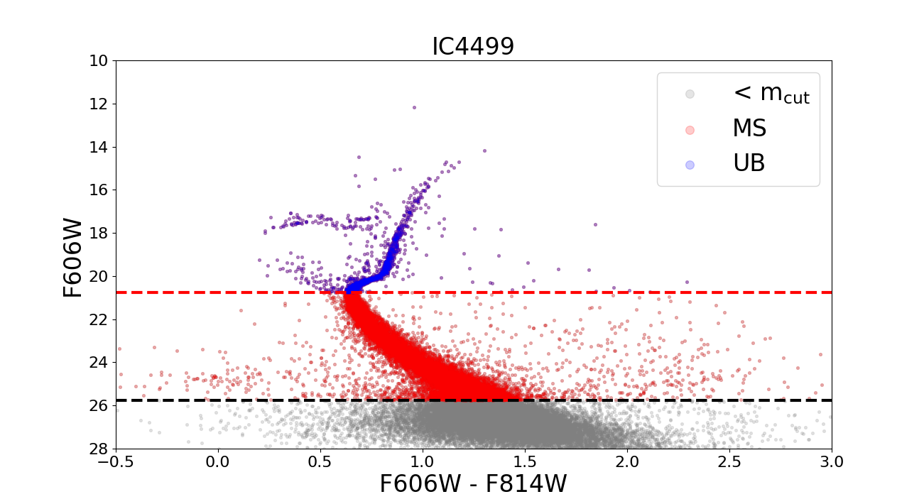
Here we attempt to reduce the high dimensionality of the parameter space using a different approach. While the large number of stars can be a liability in terms of computational cost for traditional Bayesian approaches, we turn it to our advantage, especially in the most populated part of the color-magnitude diagram. For each isochrone of the stellar model, there are a number of equivalent evolutionary points (EEPs) (see line 5 of Table 1) associated with an initial stellar mass. Each EEP has a counterpart in every isochrone, making it possible to identify specific points in the color-magnitude diagram across different isochrones, e.g., the MSTOP. In other words, the isochrone profile in the color-magnitude diagram is sampled by EEPs (which are “universal” across different isochrones) obtained for different adopted values of the parameters of interest. This is the reason why, as it is well known, the interpolation between evolution tracks is greatly simplified by interpolating instead directly between EEPs. Since we are not interested in the initial mass of stars, we do not model each star independently and exploit the benefits of the EEPs working directly with them, as provided by the relevant photometry files. This reduces the dimensionality of our analysis to just the five GC parameters described in the previous section.
We divide the “functional” magnitude interval into two parts as illustrated in Figure 1: the part below the MSTOP, which we refer to as MS for main sequence, and the part above, which we refer to as UB for upper branch. The large spread of colors at low magnitudes introduces a lot of noise, which slows down significantly the convergence of our algorithm without adding, in practice, any useful additional signal. For this reason, on top of the selection cuts described in Sec. 2, we apply a potentially more stringent upper magnitude cut. In practice, for the 68 clusters in our catalog we choose an upper cut magnitude value
| (3.1) |
where is the magnitude corresponding to the MSTOP. In fact, for some GCs going 5 magnitudes below the MSTOP would cause to include noisy data. With this choice we limit the cut for those GCs to . Our findings are not sensitive to the details of this cut as long as the noisy, dim part of the color-magnitude diagram is removed, and enough EEPs in the main sequence are retained, which is what we ensure here.
3.1 Main sequence
We proceed to bin in magnitude the sample of stars belonging to the main sequence; these bins should be thin enough so that the isochrone can be approximated as linear in each bin, yet with number of stars per bin large enough to satisfy the central limit theorem. Given the large number of stars in the MS (as illustrated in the bottom panel of Figure 1), these two conditions are fulfilled for all GCs. In practice, we use bins in the magnitude interval for the MS with constant width of 0.2 mag, which yields a maximum of 25 bins and a minimum of 20 for the GCs in our catalog. The number of stars per bin is proportional to the number of stars in the GC and ranges from several hundreds to several thousands. It is then justified to assume that the scatter in color of stars inside each magnitude bin follows a Gaussian distribution centered on the true underlying isochrone. This simplification (akin to a coarse-graining in the color-magnitude diagram, and thus to a data-compression) alone allows us to decrease the effective size of the data set, and thus, compared to previous approaches, to reduce the number of model parameters for this part of the analysis: we have 5 parameters, and number of data points. The main peak of the distribution of star positions along the color axis in each bin, indexed by , should be, and is, well approximated by a Gaussian distribution (see Figure 9 in Appendix C for an illustration). Bins where the distribution cannot be fit by a unimodal Gaussian – a possible sign of multiple populations – are removed from the analysis. This always happens at the faint end of the main sequence (except for three clusters for which one to two bins are removed), even after the cut from Equation (3.1). For this reason we use instead the median of the distribution. It allows us to keep the maximum of 25 bins while taking into account the effect of the multiple population. The median value is almost identical to the Gaussian mean and larger error bars are a reasonable trade-off for outliers. More details are presented in Appendix C. The color at bin center for each magnitude bin is defined by the median. Since the main sequence in the color-magnitude diagram is not perfectly vertical, we rescale the error by where is the standard error of the median and is the angle between the data orientation and the vertical axis inside bin as detailed in Appendix C (in particular see Figure 10 in the Appendix). This correction is very small and always well below 4%. Figure 2 shows an example of this binning for GC IC4499, along with the corresponding and .
Assuming that bins are uncorrelated (which given the small observational errors in the star magnitudes is a fair assumption), the logarithm of the likelihood is defined as
| (3.2) |
where is the theoretical isochrone color interpolated at the center of bin , and is the number of bins considered in the analysis (i.e., after removing the bins with bimodal color distributions).

3.2 Upper branch
In addition to the main sequence, we consider stars belonging to the Upper Branch (UB) i.e., stars brighter than the MSTOP. We bin the magnitude interval as we did for the main sequence. However, in this case, the number of stars is not large enough to support the central limit theorem for small magnitude bins; in addition we expect that the measurement will be highly sensitive to outliers. Therefore, we cannot fit the color distribution to a Gaussian function as done for the MS. Instead, we apply these three prescriptions:
- •
Since DSED isochrones do not include stages beyond the tip of the red giant branch –i.e., do not include EEPs belonging to the Horizontal branch and the asymptotic giant branch–, we mask out all the bins which correspond to stars (and EEP) that do not belong to either the sub-giant branch or the red giants.
- •
Since the estimation of the mean is easily contaminated by outliers, we use the median color instead in each bin as an estimate for . In fact, we expect that the color errors follow a Gaussian distribution, and that the outliers are stars that are not part of the GC main sequence of upper branch (our target sample). If we could select only stars that belong to our target sample, they would follow a Gaussian distribution. In practice, using the median down weights the contribution of outliers on the estimate of the central value of the distribution. Therefore, it provides a good estimate of the mean value of the distribution of the target sample; here we assume that the resulting distribution matches the target distribution and can be assumed to be Gaussian.
- •
We use the error of the median for normal distributions , where is the regular standard deviation in bin .
This is illustrated in Figure 3. In this figure, for a representative GC, IC4999, the stars in the color-magnitude diagram are shown as grey points, the excluded bins are shaded, the red points show the , and the error bars show the .
Finally the likelihood is also taken to be Gaussian as in Eq. 3.2, with the only differences of being the median value at bin center, and the associated error for bin . We are aware that this choice of Gaussian likelihood is not as well motivated as for the MS. Nevertheless we note here that other systematic uncertainties (see section 4.1) are likely larger than the one introduced by this approximation.
3.3 Multiple populations and magnitude cut
For the sake of simplicity in the analysis, we assume that parameters such as age, metallicity and distance are common to all stars belonging to the GC. Nonetheless, GCs can be more complex and host distinct populations. Multiple populations in GCs is an active research area (see e.g., [23] for a review). It is important to note that multiple populations do not necessarily have different ages, they may have e.g., different element abundances. Moreover, the effects of multiple populations are minimized for the filters used to create the catalog ( and ; see Ref. [23] and references therein). When we apply our analysis to GCs known to host multiple populations to quantify the effect that this might have in the inferred constraints, we find that having multiple populations introduces an additional widening in the marginalized inferred age, as well as multiple peaks for the metallicities. GCs with multiple populations have a manifestly multi-modal posterior distribution where additional local maxima may appear. We find that the magnitude cut (see Equation 3.1) we impose helps to reduce the sensitivity to secondary populations, i.e., it suppresses the secondary local maxima, but leave the global maximum unaffected. This is because it is easier to see multiple population in the faint end of the MS; at brighter magnitudes, the two populations blend. Nevertheless, the posterior distributions obtained for some GCs are still multi-modal. Masking out bins where the distribution is markedly multimodal further minimize this effect. Any residual multi-modality is blended with the main maximum and thus effectively contributes to growing the errors. The way we deal in practice with the multi-modality of these secondary local maxima is developed further in Sec. 4.
4 Parameter inference
We assume that the two parts (MS and UB) of the “functional” magnitude interval considered are independent. The total log-likelihood, , is then .
The parameters that we vary are: age, metallicity [Fe/H], absorption, distance and enhancement [/Fe]. In order to ensure that we remain inside the interpolation domain of the stellar model, we use uniform priors corresponding to the intersection of the parameter-space volumes of the stellar model (in our case this corresponds to the prior region of DSED see Table 1). These are: [1,15] Gyr for the age, [-2.5,0.5] dex for metallicity, (0,3] for absorption, (0,) for distance and [-0.2,0.8] for [/Fe].
In addition, we adopt gaussian priors on the metallicity, distance modulus, absorption and [/Fe] as follows. For the metallicity, enhancement and distance the priors are centered around estimates from the literature for each globular cluster (see Ref. [14]). For 65 clusters the extinction estimates are based on the two catalogs of Refs [24, 25]; however, for three globular clusters (NGC 6121, NGC 6144, NGC 6723) we use instead values from more recent literature (Refs [26, 27, 28] respectively) since the quality of the fit and the posterior were unacceptable when using the catalogs estimates.
We adopt dex for the width of the Gaussian priors for the metallicity, based on spectroscopic measurements, corresponding to twice the typical errors reported in Ref. [3]).88 8 In principle, this prior could be more stringent, following Ref. [29]. However we decide not to do this here, and explore a wider range in metallicy. The width adopted for the distance modulus prior is from Gaia/Hipparcos indirect distances, 2-3 times the typical errors reported in Ref. [3, 4]. We assume a dispersion on the reddening , in agreement with Ref. [4], which translates into Gaussian priors on absorption with following the Cardelli et al. [30] relation. For [/Fe] we adopt a prior of which is equivalent to the sampling step of the DSED stellar grid.
Unlike the priors on metallicity or distance which are conservative compared to recent literature, the prior on absorption needs to be restrictive to reduce the degeneracy between age and absorption. Even though it may appear narrow, one should bear in mind that this parameter is usually kept fixed in other analyses in the literature.99 9 We have also explored relaxing the metallicity prior by increasing the width of the gaussian by a factor few. We find that this more conservative choice does not affect the final results of the inferred age (, ) as statistical errors remain below the systematic ones.
For some clusters, the posterior distribution is cut by the 15 Gyr age limit imposed by the grid of the stellar models, but even in these cases the peak of the distribution is always well determined and the cut happens at the level, hence the effect on the results can be kept under control.
Given the nature of the problem (degeneracy between the age, distance and the metallicity), the nature of the data (possible presence of multiple populations), and the nature of the likelihood calibration (we fit, at the same time, the MS and the UB, where, in principle, each might favor a different region of the parameter space and be affected by different degeneracies), we expect that the posterior distribution might be multi-modal. In this case, the standard emcee sampler may be inefficient.
Existing methodologies to handle multi-modal distributions include slicing the parameter space and combining the results afterwards, or techniques like parallel-tempering Monte Carlo Markov chains where the chains are run at different temperatures, which makes it easier to the chains to communicate and thus “move” between peaks and low likelihood regions. The first approach is expensive in terms of computational cost and we found the second one not efficient in our case. Parallel tempering MCMC will move the “coldest” chains to a formal global maximum which is however in a non-physical region of parameter space (ages 15 Gyr and very low metallicities [Fe/H] -2.3 dex). We explain this tendency as follows. At high ages and low metallicities the evolutionary tracks in the color magnitude diagram become very similar to each other (as shown in Figure 8 in Appendix A). In other words, there is a lot of prior volume to explore, and therefore the chains tend to spend a lot of time there. This is an artifact of the prior probability distribution chosen.
One of the consequences of having multi-modal posterior distributions with several local maxima of the likelihood and one global maximum, and using the standard affine invariant emcee sampler, is a low acceptance fraction. This is especially significant if the modes are well separated, i.e., if the separation between modes is much larger than the width of the distribution around the maxima. Indeed, only a small fraction of MCMC steps, close to the likelihoods peaks are accepted. One possibility to bypass this technical difficulty may involve re-parametrization [31] or non-uniform priors, in addition to using stronger Gaussian priors on the metallicity.
We decided to stick to the standard emcee sampler and increased the number of chains to improve the number of accepted steps. We run 100 chains (or walkers for emcee) for 5000 steps (several times the autocorrelation length) with a burn-in phase of 500 steps. This set up returns a suitable and stable acceptance rate. For multimodal distribution, the initialization of the chains can be a important factor. We tested two configurations (a tiny Gaussian ball centered on estimates from the literature see Ref. [14] and a uniform distribution with boundaries matching the uniform priors. Both gave consistent results and we kept the second configurations as it is more objective. We have also made several convergence tests on a subset of clusters varying the number of walkers and increasing the steps of each of them (from 100 to 700 walkers for up to 100,000 steps) and found that this does not change the results.
We report the error on the parameters as the highest posterior density interval (also sometimes referred to as minimum credible interval) at a given confidence level. Note that for non-symmetric distributions (such as those we have here) these errors are not necessarily symmetric.
4.1 Systematic uncertainties
In our approach, all the parameters that describe the GCs (age, distance, metallicity, [/Fe] and extinction) are determined directly from the data. While HST photometry does have some remaining systematic uncertainty, this is minute compared to the uncertainty associated with the theoretical stellar model (see below). We estimate the systematic uncertainties in the ages of GCs induced by the theoretical stellar model using the recipe in Table 2 of Ref. [4]. To our knowledge, this is the most rigorous approach among stellar model-building to estimate the systematic uncertainties using the “known-unknowns”. Inspection of Table 2 in Ref. [4] shows that the main systematic uncertainty is due to the use of mixing length theory to model convection in the 1D stellar models. The other dominant systematic uncertainty is related to reaction rates and opacities.1010 10 Rotation is another source of systematic uncertainty, as the rotation speed of stars in GCs is unknown. However, the main effect of rotation is to alter the depth of the convection zone. Given that we have explored a wide range of values of the mixing length parameters, the effect of rotation is effectively included in our systematic budget estimation. Everything else is subdominant, thus the combined effect these two components captures well the extent of systematic errors.
Mixing-length theory1111 11 In Appendix D we give a brief description of mixing-length theory. has two parameters: the mixing-length parameter (i.e., roughly how much the convection cells travel before they break up), and the overshoot parameter (how much the convective cell travels beyond the equilibrium condition). Of these two, the second one is unimportant for low-mass stars such as those in GCs. These two parameters dominate the uncertainty in stellar model building; the uncertainties in nuclear reactions are at the % level.
In principle, changes in the mixing length do not alter the lifetime of the star, see discussion in page 725, of Ref. [32]. The effect on the inferred age arises from degeneracies with metallicity. In this work the metallicity is strongly constrained so that, in principle, the effect of mixing length uncertainties could be reduced significantly.
In fact, the mixing length parameter is usually calibrated from fits to the Sun, but astro-seismology from other stars at different evolutionary stages indicates a spread of values between 1.0 and 1.7. Thus, the results from observations of the Sun are extrapolated to stars belonging to GCs, but adopting the full spread of mixing length parameter values to quantify the systematic uncertainties. However, a better estimation of systematic uncertainties related with the mixing length parameter is possible. As shown in Ref. [10], not only the morphology of the red giant branch can be used to constrain the value of the mixing length, but also all the GCs analysed in Ref. [10], had the same value for the mixing length and showed no star-to-star variation of the mixing length parameter. Therefore, the morphology of the red giant branch is sufficient to constrain the mixing length, once the metallicity is constrained, without the need to rely on the solar calibration. Thus, potentially, for the present study, as the metallicity can be constrained from the lower main sequence as well as the sub-giant branch (see Figure 8), the upper giant branch could be used to determine the value of the mixing length as done in Ref. [10]. This approach would require adding the mixing length parameter as an extra free parameter in our analysis; we leave this for future work.
Here instead we prefer to be conservative and use the full range for the mixing length considered in Ref. [4] (i.e., between 1.0 and 1.7), which is conservative because the study of Ref. [10] showed that fits to the position of the red giant branch with known metallicity indicate no significant spread in mixing length parameter. These fits recover a value of 1.6, well in agreement with results from calibration to the Sun. To estimate the error in ages due to mixing length variations over the full conservative interval, we use the stellar models of Ref. [32], and in particular the fitting formulas therein. This yields a 0.3 Gyr age uncertainty.
In addition to this we add an extra 0.2 Gyr to account for uncertainties in reaction rates and opacities, as from Table 2 of Ref. [4]. In total, we have a 0.5 Gyr uncertainty budget due to systematic effects in stellar modeling.
Note that in the standard MSTOP approach, another systematic uncertainty to account for would be the value of [/Fe], which in general is not known and is assumed to be between . However, in our approach, this is not the case as this is a parameter of the model: its value is directly constrained by the analysis and its uncertainty is therefore already included in our marginalized errors.
5 Results
We apply the methodology presented in previous sections to our catalog of 68 GCs. Two-dimensional marginalized posteriors for all pairs of parameters can be found for a representative GC in Appendix F. Figure 4 shows our main results (see also Appendix E and Tables 3 and 4). We present marginalized constraints on the absolute age, metallicity, distance, absorption and [/Fe] of each GC assuming the DSED model. The -axis in each panel shows the cluster id following the same order as in table 3. The gray horizontal areas show the hard priors imposed by the stellar models domain in parameter space and the gray vertical band (when reported) illustrates the width the gaussian prior adopted (see Sec. 4). We find no correlation between age and distances, absorption or [/Fe]. In particular the absorption values are low and the distribution presents a scatter that is not correlated with the age. On an individual cluster-basis the constraints on [/Fe] are very weak, however values of [/Fe] are typically disfavored. A comparison with Dotter et al. [14] spectroscopic measurements can be found in Appendix F.
In Figure 5 we compare our inferred constraints with the findings of Ref. [4] for the 22 GCs in common. It is interesting to note the good agreement obtained for the metallicity estimates of [Fe/H]. Our distances, using information from the color-magnitude diagram and only very weak priors, are in reasonable agreement with those obtained Ref. [4], which rely on external information (GAIA parallaxes and accurate distance to nearby dwarf stars). However, we find a small shift as our determination of distances is pc smaller on average. This small discrepancy arises because the analysis in Ref. [4] assumes a fixed extinction value, while we treat extinction as a free parameter to be constrained by the data and marginalized over. For the ages determination the agreement is within 68% confidence level uncertainties. From the first panel of Figure 5 it is possible to appreciate that the errors from this study are smaller that those of Ref. [4] even when Ref. [4] uses additional external information, not used here. This illustrates the advantage of considering regions of the color-magnitude diagram beyond the main sequence.
The use of the full color-magnitude diagram, along with the adoption of the priors motivated in sec. 4, enables us to break the age–distance–metallicity degeneracy. In particular, the breaking of the age-metallicity degeneracy is visualized in Appendix A where we show how the isochrones and the color magnitude diagram change in response to variations of these parameters.
5.1 The age of the oldest GCs

On average, the oldest GCs are those expected to be more metal poor. Here we consider two metallicity cuts as a way to select the oldest GCs: [Fe/H] as adopted in Ref. [33] – leaving 11 clusters – and [Fe/H] – leaving 38 clusters– . We estimate the age distribution for these two samples by multiplying the individual bayesian posteriors (see Fig. 6).
For [Fe/H] this yields , while for [Fe/H] we obtain . The first uncertainty is the statistical uncertainty while the second uncertainty is the systematic one, as calculated in Sec. 4.1. The results for the two cuts are very consistent; as expected, the additional 27 clusters in the [Fe/H] cut reduce the statistical error significantly; here we therefore adopt the [Fe/H] cut due to the increased statistical power.
5.2 From globular cluster ages to the age of the Universe
The age of the oldest stars sets a lower limit for the age of the Universe. These stars and the oldest GCs formed at a redshift . Hence, it is possible to estimate the age of the Universe from the age of the oldest GCs adding a formation time , corresponding to the look back time at .
As argued in Ref. [33], it is possible to estimate the probability distribution of by considering that the first galaxies are found at and a significant number of galaxies are found at . Many of these galaxies contain stellar populations that indicate that star formation started at [34, 35, 36]; is thus assumed to be . Both theoretically [37, 38, 39, 40, 41] and observationally [42] GC seem to form at . On the other hand, GCs could not have formed before the start of reionization which is estimated to happen around . Ref. [33] includes a computation of the probability distribution of marginalizing over , and , with varying between and . The resulting distribution depends very weakly on cosmology for reasonable values of the cosmological parameters, and very weakly on the choice of provided . Here we estimate the full probability distribution of by performing a convolution of the posterior probability distribution for as provided in § 5.1 and the probability distribution of from Ref. [33] for which we provide a fitting formula in appendix G.
We find at 68% confidence level. The resulting posterior distribution for the age of the Universe is presented in Figure 7. The solid black line is the result including only statistical errors, the dashed line is obtained by fitting this distribution with two gaussians with the same maximum but independent variances for the two sides (dotted line), and then adding the systematic error in quadrature (dashed line). For reference the blue thin line shows the constraint inferred from CMB observations from Planck, assuming the CDM model [43].
6 Summary and Conclusions
Resolved stellar populations of GCs provide an excellent data set to constrain the age of the Universe, which in turn is a key parameter in cosmology governing the background expansion history of the Universe. Since the mid 90’s, estimates of the ages of GCs have been in the range Gyr consistently (see e.g. Ref. [10]). With current improvements in observational data and stellar modeling, it is possible to decrease the uncertainty on the ages by a factor 4. Given the high-quality of data obtained by HST and the improvement in the accuracy of stellar models, we have attempted to estimate the physical parameters of GCs including their age, using as many features as possible in their color-magnitude diagrams.
It is well known that the MSTOP is very sensitive to the GC’s age; however, it is also sensitive to distance, metallicity, and other parameters, due to significant degeneracies in parameter space. However, degeneracies can be in large part lifted if other features of the color-magnitude diagram are exploited (see Appendix A). In this paper, we have analyzed a sample of 68 ACS/HST globular clusters using most of the information in the color-magnitude diagram: specifically, the main sequence and red giant branch. We have developed a Bayesian approach to perform an analysis of each GC, varying simultaneously their age, distance, metallicity, [/Fe] and reddening adopting physically-motivated priors based on independent measurements of distances, metallicities and extinctions found in recent literature. Our obtained posteriors yield constraints that are fully compatible with previous, and independent, values in the literature.
The average age of the oldest (and most metal poor) GCs is Gyr. The systematic errors are due to theoretical stellar model uncertainties and in particular uncertainties in the mixing length, reaction rates and opacities. Systematic errors are now bigger than the statistical error, once constraints from several objects are combined. Hence, to make further progress, uncertainties in stellar model-building should be addressed.
This determination can be used to estimate the Universe absolute age by taking into account the look back time at the likely redshift of formation of these objects. We find the age of the Universe as determined from stellar objects to be at 68% confidence level. The statistical error is 1.2%; the error budget is dominated by systematic uncertainties on the stellar modeling. The prospect of determining the age of the Universe with an accuracy competitive with current cosmology standards, may serve to motivate an effort to reduce uncertainties in stellar-model building. This will be addressed in future work. The statistical uncertainty in is now sufficiently small to warrant comparison to the CMB model-dependent inferred age, which is one of the most accurately quantities inferred from the CMB [44]. Thus comparing the CMB derived value to independent astrophysical estimates can yield precious insights into possible new physics, or support the CDM model. Our determined value of is fully compatible with the inferred value from the Planck mission observations assuming the CDM model.
Acknowledgments
We thank the stellar modelers for making their stellar models publicly available. We thank the anonymous referee for an useful and constructive report. We also thank David Nataf for very useful feedback. This work is supported by MINECO grant PGC2018-098866-B-I00 FEDER, UE. JLB is supported by the Allan C. and Dorothy H. Davis Fellowship. JLB has been supported by the Spanish MINECO under grant BES-2015-071307, co-funded by the ESF, during part of the development of this project. LV acknowledges support by European Union’s Horizon 2020 research and innovation program ERC (BePreSySe, grant agreement 725327). The work of BDW is supported by the Labex ILP (reference ANR-10-LABX-63) part of the Idex SUPER, received financial state aid managed by the Agence Nationale de la Recherche, as part of the programme Investissements d’avenir under the reference ANR-11-IDEX-0004-02; and by the ANR BIG4 project, grant ANR-16-CE23-0002 of the French Agence Nationale de la Recherche. The Center for Computational Astrophysics is supported by the Simons Foundation.
References
- [1] M. Catelan, The ages of (the oldest) stars, in Rediscovering Our Galaxy, C. Chiappini, I. Minchev, E. Starkenburg and M. Valentini, eds., vol. 334 of IAU Symposium, pp. 11–20, Aug., 2018, DOI [1709.08656].
- [2] D. R. Soderblom, The Ages of Stars, ARAA 48 (2010) 581 [1003.6074].
- [3] D. A. Vandenberg, M. Bolte and P. B. Stetson, The Age of the Galactic Globular Cluster System, ARAA 34 (1996) 461.
- [4] E. M. O’Malley, C. Gilligan and B. Chaboyer, Absolute Ages and Distances of 22 GCs Using Monte Carlo Main-sequence Fitting, ApJ 838 (2017) 162 [1703.01915].
- [5] C. B. Haselgrove and F. Hoyle, A preliminary determination of the age of type II stars, MNRAS 116 (1956) 527.
- [6] A. R. Sandage and M. Schwarzschild, Inhomogeneous Stellar Models. II. Models with Exhausted Cores in Gravitational Contraction., ApJ 116 (1952) 463.
- [7] R. Jimenez and P. Padoan, A New Self-consistency Check on the Ages of Globular Clusters, ApJL 463 (1996) L17.
- [8] P. Padoan and R. Jimenez, Ages of Globular Clusters: Breaking the Age-Distance Degeneracy with the Luminosity Function, ApJ 475 (1997) 580 [astro-ph/9603060].
- [9] R. Jimenez and P. Padoan, The Ages and Distances of Globular Clusters with the Luminosity Function Method: The Case of M5 and M55, ApJ 498 (1998) 704 [astro-ph/9701141].
- [10] R. Jimenez, P. Thejll, U. G. Jorgensen, J. MacDonald and B. Pagel, Ages of globular clusters: a new approach, MNRAS 282 (1996) 926 [astro-ph/9602132].
- [11] R. Wagner-Kaiser, A. Sarajedini, T. von Hippel, D. C. Stenning, D. A. van Dyk, E. Jeffery et al., The ACS survey of Galactic globular clusters - XIV. Bayesian single-population analysis of 69 globular clusters, MNRAS 468 (2017) 1038 [1702.08856].
- [12] C. L. Sahlholdt, S. Feltzing, L. Lindegren and R. P. Church, Benchmark ages for the Gaia benchmark stars, MNRAS 482 (2019) 895 [1810.02829].
- [13] A. Sarajedini, L. R. Bedin, B. Chaboyer, A. Dotter, M. Siegel, J. Anderson et al., The ACS Survey of Galactic Globular Clusters. I. Overview and Clusters without Previous Hubble Space Telescope Photometry, AJ 133 (2007) 1658 [astro-ph/0612598].
- [14] A. Dotter, A. Sarajedini, J. Anderson, A. Aparicio, L. R. Bedin, B. Chaboyer et al., The ACS Survey of Galactic Globular Clusters. IX. Horizontal Branch Morphology and the Second Parameter Phenomenon, ApJ 708 (2010) 698 [0911.2469].
- [15] T. D. Morton, isochrones: Stellar model grid package, Mar., 2015.
- [16] A. Dotter, MESA Isochrones and Stellar Tracks (MIST) 0: Methods for the Construction of Stellar Isochrones, ApJS 222 (2016) 8 [1601.05144].
- [17] J. Choi, A. Dotter, C. Conroy, M. Cantiello, B. Paxton and B. D. Johnson, Mesa Isochrones and Stellar Tracks (MIST). I. Solar-scaled Models, ApJ 823 (2016) 102 [1604.08592].
- [18] A. Dotter, B. Chaboyer, D. Jevremović, V. Kostov, E. Baron and J. W. Ferguson, The Dartmouth Stellar Evolution Database, ApJS 178 (2008) 89 [0804.4473].
- [19] E. Simpson, R. E. Hills, W. Hoffman, S. A. Kellman, J. Morton, Erwin, F. Paresce et al., Studies in Stellar Evolution.IX. Theoretical Isochrones for Early-Type Clusters, ApJ 159 (1970) 895.
- [20] G. Bertelli, R. Betto, A. Bressan, C. Chiosi, E. Nasi and A. Vallenari, Theoretical isochrones with convective overshoot., A&ASS 85 (1990) 845.
- [21] G. Bertelli, A. Bressan, C. Chiosi, F. Fagotto and E. Nasi, Theoretical isochrones from models with new radiative opacities., A&ASS 106 (1994) 275.
- [22] E. L. Fitzpatrick, Correcting for the Effects of Interstellar Extinction, PASP 111 (1999) 755 [astro-ph/9809387].
- [23] N. Bastian and C. Lardo, Multiple Stellar Populations in Globular Clusters, ARAA 56 (2018) 83 [1712.01286].
- [24] W. E. Harris, A Catalog of Parameters for Globular Clusters in the Milky Way, Aj 112 (1996) 1487.
- [25] C. M. Dutra and E. Bica, Foreground and background dust in star cluster directions, aap 359 (2000) 347 [astro-ph/0005108].
- [26] B. Hendricks, P. B. Stetson, D. A. VandenBerg and M. Dall’Ora, A New Reddening Law for M4, Aj 144 (2012) 25 [1204.5719].
- [27] R. K. Neely, A. Sarajedini and D. H. Martins, CCD Photometry of the Galactic Globular Cluster NGC 6144, Aj 119 (2000) 1793.
- [28] J.-W. Lee, M. López-Morales, K. Hong, Y.-W. Kang, B. L. Pohl and A. Walker, Toward a Better Understanding of the Distance Scale from RR Lyrae Variable Stars: A Case Study for the Inner Halo Globular Cluster NGC 6723, Apjs 210 (2014) 6 [1311.2054].
- [29] E. Carretta, A. Bragaglia, R. Gratton, V. D’Orazi and S. Lucatello, Intrinsic iron spread and a new metallicity scale for globular clusters, aap 508 (2009) 695 [0910.0675].
- [30] J. A. Cardelli, G. C. Clayton and J. S. Mathis, The Relationship between Infrared, Optical, and Ultraviolet Extinction, ApJ 345 (1989) 245.
- [31] A. Kosowsky, M. Milosavljevic and R. Jimenez, Efficient cosmological parameter estimation from microwave background anisotropies, PRD 66 (2002) 063007 [astro-ph/0206014].
- [32] R. Jimenez and J. MacDonald, Stellar evolutionary tracks for low-mass stars, MNRAS 283 (1996) 721.
- [33] R. Jimenez, A. Cimatti, L. Verde, M. Moresco and B. Wandelt, The local and distant Universe: stellar ages and H0, JCAP 2019 (2019) 043 [1902.07081].
- [34] T. Hashimoto, N. Laporte, K. Mawatari, R. S. Ellis, A. K. Inoue, E. Zackrisson et al., The onset of star formation 250 million years after the Big Bang, Nature 557 (2018) 392 [1805.05966].
- [35] V. Strait, M. Bradač, D. Coe, L. Bradley, B. Salmon, B. C. Lemaux et al., Stellar Properties of z 8 Galaxies in the Reionization Lensing Cluster Survey, ApJ 888 (2020) 124 [1905.09295].
- [36] C. Binggeli, E. Zackrisson, X. Ma, A. K. Inoue, A. Vikaeus, T. Hashimoto et al., Balmer breaks in simulated galaxies at , MNRAS 489 (2019) 3827 [1908.11393].
- [37] P. Padoan, R. Jimenez, Raul and B. Jones, On star formation in primordial protoglobular clouds, MNRAS 285 (1997) 711 [astro-ph/9604055].
- [38] M. Trenti, P. Padoan, R. Jimenez, The Relative and Absolute Ages of Old Globular Clusters in the LCDM Framework, ApJL 808 (2015) L35 [1502.02670].
- [39] N. Choksi, O. Gnedin and H. Li, Formation of globular cluster systems: from dwarf galaxies to giants,MNRAS 480 (2018) 2343 [1801.03515].
- [40] M. Reina-Campos,The origin of metal-poor and metal-rich globular clusters in E-MOSAICS, , Proceedings of the International Astronomical Union14 (2019) 147 [astro-ph/0109232].
- [41] J. M. D. Kruijssen, The minimum metallicity of globular clusters and its physical origin – implications for the galaxy mass–metallicity relation and observations of proto-globular clusters at high redshift, MNRASL486 (2019) L20 [1904.09987].
- [42] D. A. Forbes, N. Pastorello, A.J. Romanowsky, C. Usher, J.P. Brodie, J. Strader, SLUGGS survey: inferring the formation epochs of metal-poor and metal-rich globular clusters,MNRASL452 (2015) 1045 [1506.06820].
- [43] Planck Collaboration, N. Aghanim, Y. Akrami, M. Ashdown, J. Aumont, C. Baccigalupi et al., Planck 2018 results. VI. Cosmological parameters, arXiv e-prints (2018) arXiv:1807.06209 [1807.06209].
- [44] L. Knox, N. Christensen and C. Skordis, The Age of the Universe and the Cosmological Constant Determined from Cosmic Microwave Background Anisotropy Measurements, ApJL 563 (2001) L95 [astro-ph/0109232].
- [45] R. Kippenhahn and A. Weigert, Stellar Structure and Evolution. 1990.
Appendix A Test of sensitivity of the color-magnitude diagram to model parameters
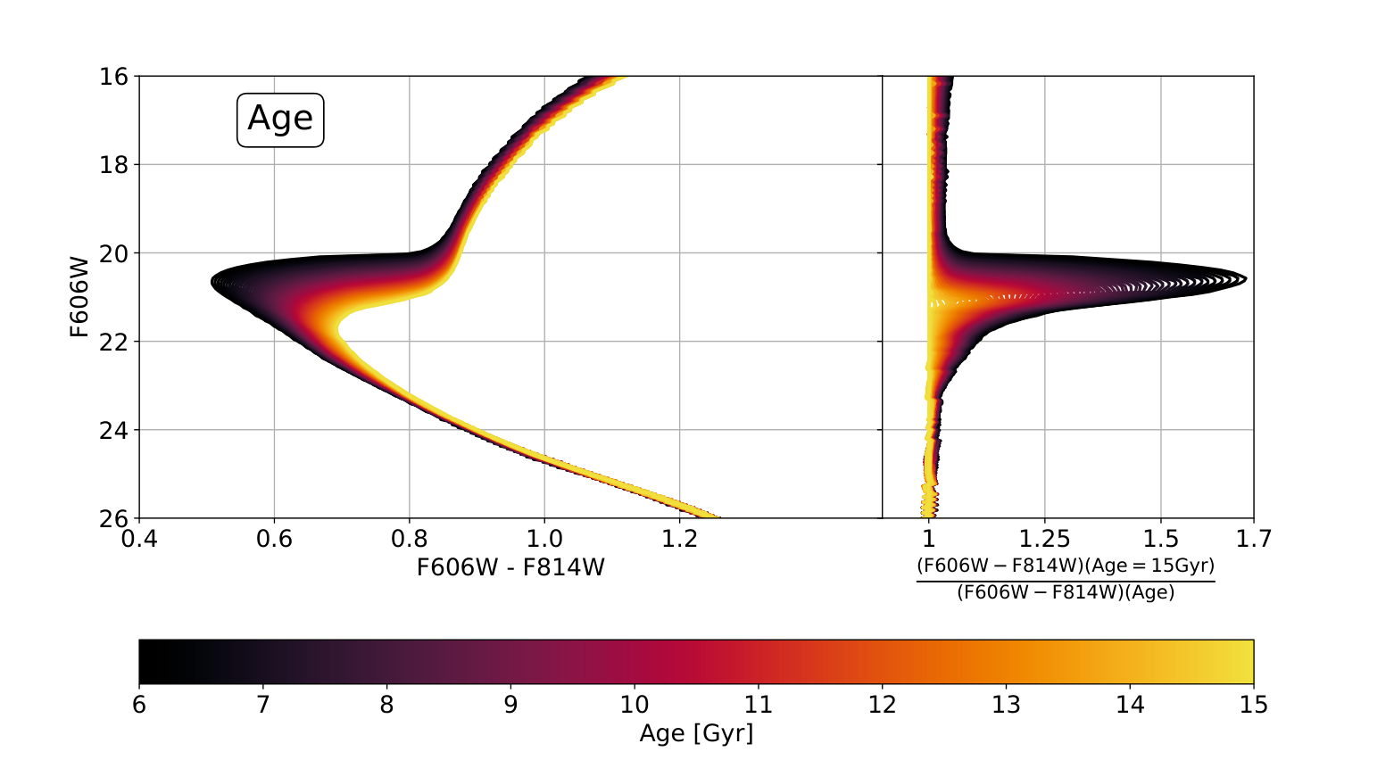
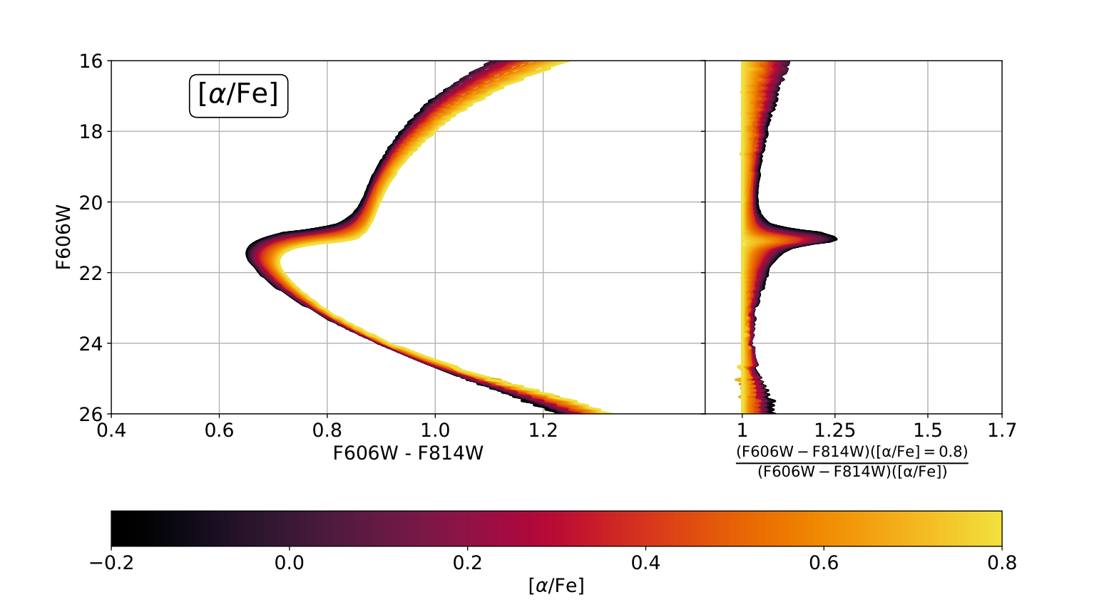
In this appendix we explore the dependence of the isochrones in the color-magnitude diagram of a GC on the model parameters. On top of illustrating the sensitivity of different sections of the evolutionary track to these parameters, this exercise will allow us to convey how parameter degeneracies can be lifted by considering regions above the main sequence. We start from a common set of parameters (based on estimates from literature, see Ref. [14]) and vary one parameter at a time, while we keep the others fixed. As we vary the parameter of interest, we compare the color at the interpolated magnitudes for each isochrone.
We show the corresponding comparison as function of age, metallicity, and [/Fe] in Figure 8. The figure clearly shows that most of the sensitivity to age is around the MSTOP, but if only this point is used, age is degenerate with metallicity. However, both the red giant branch and the lower main sequence are sensitive to metallicity, significantly more than to age. This explains why using more features of the color-magnitude diagram breaks the degeneracy. Further, the whole color-magnitude diagram has a different sensitivity to [/Fe] than to [Fe/H]. Thus, with enough signal-to-noise, both quantities can be constrained in a joint analysis.

Appendix B Globular clusters properties after the cuts
| Cluster name | Total number of stars | Stars with magnitude | percentage of remaining stars |
|---|---|---|---|
| arp2 | 23010 | 10611 | 46 |
| ic4499 | 61931 | 33938 | 54 |
| lynga7 | 44927 | 27496 | 61 |
| ngc0104 | 140016 | 113700 | 81 |
| ngc0288 | 26814 | 14465 | 53 |
| ngc0362 | 111393 | 71978 | 64 |
| ngc1261 | 97780 | 61767 | 63 |
| ngc1851 | 130655 | 82732 | 63 |
| ngc2298 | 20288 | 13453 | 66 |
| ngc2808 | 277727 | 214443 | 77 |
| ngc3201 | 31908 | 17056 | 53 |
| ngc4147 | 19717 | 13977 | 70 |
| ngc4590 | 60058 | 33182 | 55 |
| ngc4833 | 60889 | 41720 | 68 |
| ngc5024 | 222899 | 132605 | 59 |
| ngc5053 | 23957 | 11104 | 46 |
| ngc5139 | 300622 | 206535 | 68 |
| ngc5272 | 161342 | 106494 | 66 |
| ngc5286 | 190379 | 131490 | 69 |
| ngc5466 | 29776 | 13660 | 45 |
| ngc5904 | 108602 | 73235 | 67 |
| ngc5927 | 96349 | 69333 | 71 |
| ngc5986 | 148963 | 100314 | 67 |
| ngc6093 | 125128 | 88784 | 70 |
| ngc6101 | 67032 | 33715 | 50 |
| ngc6121 | 11975 | 7070 | 59 |
| ngc6144 | 22485 | 15612 | 69 |
| ngc6205 | 138295 | 97673 | 70 |
| ngc6218 | 29767 | 20840 | 70 |
| ngc6254 | 54662 | 38462 | 70 |
| ngc6304 | 100830 | 58706 | 58 |
| ngc6341 | 129969 | 83376 | 64 |
| ngc6352 | 25779 | 14784 | 57 |
| ngc6362 | 30541 | 17724 | 58 |
| ngc6366 | 10567 | 4427 | 41 |
| ngc6388 | 310630 | 257049 | 82 |
| ngc6397 | 14277 | 9404 | 65 |
| ngc6426 | 57321 | 30576 | 53 |
| ngc6441 | 340872 | 299187 | 87 |
| ngc6496 | 22938 | 14486 | 63 |
| ngc6535 | 9590 | 3640 | 37 |
| ngc6541 | 111010 | 71816 | 64 |
| ngc6584 | 62694 | 35346 | 56 |
| ngc6624 | 62637 | 40960 | 65 |
| ngc6637 | 61801 | 44484 | 71 |
| ngc6652 | 29936 | 16586 | 55 |
| ngc6656 | 92090 | 57379 | 62 |
| ngc6681 | 48442 | 32417 | 66 |
| ngc6715 | 345989 | 270157 | 78 |
| ngc6717 | 15209 | 8235 | 54 |
| ngc6723 | 60289 | 42353 | 70 |
| ngc6752 | 47657 | 31250 | 65 |
| ngc6779 | 79381 | 47224 | 59 |
| ngc6809 | 42870 | 24095 | 56 |
| ngc6838 | 14504 | 7582 | 52 |
| ngc6934 | 81104 | 47218 | 58 |
| ngc6981 | 44154 | 29154 | 66 |
| ngc7006 | 72056 | 46216 | 64 |
| ngc7078 | 243929 | 152629 | 62 |
| ngc7089 | 227533 | 159739 | 70 |
| ngc7099 | 67053 | 37756 | 56 |
| palomar1 | 9330 | 685 | 7 |
| palomar12 | 7915 | 1981 | 25 |
| palomar15 | 22790 | 6648 | 29 |
| pyxis | 11311 | 6281 | 55 |
| ruprecht106 | 23800 | 13285 | 55 |
| terzan7 | 21637 | 7752 | 35 |
| terzan8 | 39847 | 16477 | 41 |
Appendix C Main sequence calibration
We fit the histogram of the color distribution within each magnitude bin with a unimodal Gaussian with the curve_fit routine of Scipy, for a maxfev=950000.1212 12 maxfev is set to a very large value to make sure of the non convergence of the unimodal fit. If the routine cannot find a fit to the color distribution, the bin is ignored. Otherwise, the bin is retained and the resulting Gaussian distribution is adopted. A typical example of a small contamination is shown in Figure 9: the fitting procedure captures the distribution of the main “population”.
Once the central value of the distribution is obtained (see Figure 9), we rescale the error on the distribution due to the inclination of the observed stars in the color-magnitude diagram. The orientation of the data in a MS magnitude bin is obtained by linear regression the median of the data in sub-bins, and is compared to a vertical line passing through the color of the central value (see Figure 10). The resulting angle is referred to as and it ranges between [ 0 - 10∘].
Appendix D Mixing Length Theory
Uncertainties in the modeling of convection in the envelopes of low mass stars are the main contributor to systematic uncertainties in determining stellar parameters (see Table 2 in Ref. [4]). Given the broad audience which this paper (hopefully) reaches, it is worth to briefly review mixing length theory (MLT), to understand the origin of these uncertainties.
The envelopes (about the outer 30% radius) of low mass ( M⊙) stars are fully convective and turbulent, with Reynolds number . Modeling these systems is highly challenging: in principle, a full hydro-dynamical solution should be obtained. Instead, the standard solution is to model the gradient of convective transport by the so-called MLT. Conceptually, it is a very simple approach: it assumes that a blob of gas starts at a point and continues moving until it dissolves after a certain length, the mixing length .
Consider a sphere of radius and an element of the envelope (a blob of gas) located there. After has traveled a mixing length , its increase in temperature will be
| (D.1) |
where the scale height is , is the pressure, denotes the gradient in the environment and is the gradient in the blob. Now, combining this with the equations of stellar structure, it is possible to obtain a system of five differential equations for five independent variables, namely: pressure, temperature, density, and the advective and radiative gradients. Then is an extra free parameter which needs to be determined from observations. The usual parameter that stellar modelers fit is ; this has a typical value of from fits to the Sun and to the position of red giant branch in the color-magnitude diagram of GCs [10]. The interested reader can consult the textbook by Kippenhahn & Weigert for a detailed account of all equations of stellar structure [45]. Changes for this parameter from the typical value would propagate into systematic shifts in the metallicity and age determinations.
Appendix E Parameter constraints: globular clusters
The table shows the best-fit parameters for the GC sample considered in this paper and the one-dimensional marginalized statistical uncertainties at 68% confidence level.
| Cluster name | Age [Gyr] | [Fe/H] | Distance [kpc] | [/Fe] | |
|---|---|---|---|---|---|
| arp2 | |||||
| ic4499 | |||||
| lynga7 | |||||
| ngc0104 | |||||
| ngc0288 | |||||
| ngc0362 | |||||
| ngc1261 | |||||
| ngc1851 | |||||
| ngc2298 | |||||
| ngc2808 | |||||
| ngc3201 | |||||
| ngc4147 | |||||
| ngc4590 | |||||
| ngc4833 | |||||
| ngc5024 | |||||
| ngc5053 | |||||
| ngc5139 | |||||
| ngc5272 | |||||
| ngc5286 | |||||
| ngc5466 | |||||
| ngc5904 | |||||
| ngc5927 | |||||
| ngc5986 | |||||
| ngc6093 | |||||
| ngc6101 | |||||
| ngc6121 | |||||
| ngc6144 | |||||
| ngc6205 | |||||
| ngc6218 | |||||
| ngc6254 | |||||
| ngc6304 |
| Cluster name | Age [Gyr] | [Fe/H] | Distance [kpc] | [/Fe] | |
|---|---|---|---|---|---|
| ngc6341 | |||||
| ngc6352 | |||||
| ngc6362 | |||||
| ngc6366 | |||||
| ngc6388 | |||||
| ngc6397 | |||||
| ngc6426 | |||||
| ngc6441 | |||||
| ngc6496 | |||||
| ngc6535 | |||||
| ngc6541 | |||||
| ngc6584 | |||||
| ngc6624 | |||||
| ngc6637 | |||||
| ngc6652 | |||||
| ngc6656 | |||||
| ngc6681 | |||||
| ngc6715 | |||||
| ngc6717 | |||||
| ngc6723 | |||||
| ngc6752 | |||||
| ngc6779 | |||||
| ngc6809 | |||||
| ngc6838 | |||||
| ngc6934 | |||||
| ngc6981 | |||||
| ngc7006 | |||||
| ngc7078 | |||||
| ngc7089 | |||||
| ngc7099 | |||||
| palomar1 | |||||
| palomar12 | |||||
| palomar15 | |||||
| pyxis | |||||
| ruprecht106 | |||||
| terzan7 | |||||
| terzan8 |
Appendix F Fits to ACS globular clusters
In this appendix we show fits for typical Globular clusters in the ACS sample as an illustration of the adopted methodology. For each GC the upper row of Figure 12 shows the color-magnitude diagram for the globular cluster. The gray points correspond to the individual stars, the red points show the best fit isochrone for the DSED model. The bottom row shows the marginalized posteriors of the model parameters obtained applying our analysis. The contours indicate the two-dimensional 68%, 95% and 99.7% confidence levels constraints, while the panels in the diagonal show the one-dimensional marginalized posteriors.
We also show the comparison between the best fit of the 68 Globular clusters and spectroscopic values from Dotter et al. catalog [14]. We find a very good agreement. For alsmost all the clusters, the spectroscopic value is within the 1- range of the best fit.


Appendix G Fitting formula for the distribution of
The distribution of shown in the right panel of Figure 1 of Ref. [33] can be well approximated by the following fitting formula (see Fig 13). Let indicate , and , , , , then
| (G.1) | |||||
| (G.2) | |||||
| (G.3) | |||||
| (G.4) |
