Tensor-based techniques for fast discretization and solution
of 3D elliptic equations with
random coefficients
Abstract
In this paper, we propose and analyze the numerical algorithms for fast solution of periodic elliptic problems in random media in , . We consider the stochastic realizations using checkerboard configuration of the equation coefficients built on a large lattice, where is the size of representative volume elements. The Kronecker tensor product scheme is introduced for fast generation of the stiffness matrix for FDM discretization on a tensor grid. We describe tensor techniques for the construction of the low Kronecker rank spectrally equivalent preconditioner in periodic setting to be used in the framework of PCG iteration. In our construction the diagonal matrix of the discrete Laplacian inverse represented in the Fourier basis is reshaped into a 3D tensor, which is then approximated by a low-rank canonical tensor, calculated by the multigrid Tucker-to-canonical tensor transform. The FDM discretization scheme on a tensor grid is described in detail, and the computational characteristics in terms of for the 3D Matlab implementation of the PCG iteration are illustrated. The present work continues the developments in [22], where the numerical primer to study the asymptotic convergence rate vs. for the homogenized matrix for 2D elliptic PDEs with random coefficients was investigated numerically. The presented elliptic problem solver can be applied for calculation of long sequences of stochastic realizations in numerical analysis of 3D stochastic homogenization problems for ergodic processes, for solving 3D quasi-periodic geometric homogenization problems, as well as in the numerical simulation of dynamical many body interaction processes and multi-particle electrostatics.
Key words: 3D elliptic problem solver, PDE with random coefficients, PCG iteration, low-rank tensor product approximation, Kronecker product, stochastic homogenization.
AMS Subject Classification: 65F30, 65F50, 65N35, 65F10
1 Introduction
Stochastic homogenization methods provide means for calculating the average characteristics of the structural and geometric properties of random composites. The numerical schemes for solving elliptic partial differential equations (PDEs) with random input in the form of stochastic/parametric elliptic equations have been intensively discussed in the literature [12, 2, 28, 30, 4, 5, 6, 11, 22, 31]. The theoretical analysis of quisi-periodic and stochastic/parametric problems can be found in [3, 29, 18, 10, 7] and in references therein. The rank structured tensor methods for quasi-periodic geometric homogenization methods and for the elliptic equations with highly oscillating coefficients were considered in [27, 20]. Data sparse and tensor methods for stochastic/parametric elliptic problems have been considered in [26, 28, 25, 33, 8, 9].
The main computational challenge in stochastic homogenization techniques is that the exhausting of the important information from the stochastic PDE (say, homogenized coefficient matrix or solution, and other important quantities of the stochastic process) requires a huge number of realizations, i.e. solving the target PDE many times for different stochastic input. In this respect, the valuable 3D stochastic simulations presuppose the strong requirements to the numerical efficiency of the chosen 3D elliptic problem solver.
This paper continues the development of efficient algorithms initiated by a numerical primer in [22] for fast solution of the 2D elliptic PDEs in random media, where the computational scheme for stochastic realizations using the general overlapping-type coefficient profile has been developed. The numerical study in [22] confirmed the theoretical convergence rate for the homogenized coefficients matrix in the size of representative volume element (RVE), presented in [13, 14, 16, 15]. Recall that the algorithms described in [22] are capable for 2D calculations with the number of realizations limited by the order of , implemented for coefficient configuration built on lattices with the RVE size up to . However, the 3D calculations by using a general overlapping-type profile for generation of random coefficients seem to be prohibitive for the large number of coefficient realizations over lattice structures.
In this paper, we describe the numerical scheme for discretization and solution of the -dimensional stochastic homogenization problems for , which employs the realizations over a checkerboard type configuration of the stochastic coefficient on the or lattice, respectively. In 3D case, we use the product piecewise linear finite elements on the Cartesian grids with , , assuming that the jumps in the equation coefficient are resolved by non-overlapping square subdomains (unit cells). We introduce a tensor-based scheme for fast generation of the stiffness matrix for both 2D and 3D problems by using the Kronecker product construction for assembling of the FEM stiffness matrix and for the design of the rank-structured preconditioner. In the 3D case, we construct the spectrally equivalent preconditioner by employing the explicit representation (approximation) of the 3D periodic Laplacian operator inverse in the Fourier basis in a form of a short sum of the three-fold Kronecker products of matrices, similar to [17] where the Laplacian with Dirichlet boundary conditions was considered. Algorithmically, in our construction the diagonal matrix of the discrete Laplacian inverse represented in the Fourier basis is reshaped into a 3D tensor, which is then approximated by a low-rank canonical tensor, see Lemma 4.2. This approximation is calculated by using the multigrid Tucker-to-canonical tensor transform introduced in [23, 21].
The presented numerical scheme with the checkerboard type coefficients in 2D leads to a much faster method as compared with that for overlapping coefficients [22]. This allows us to perform computations with RVE size up to for 2D problems and for the number of realizations of the order of . For 3D case the large number realizations, , for RVE size up to , discretized on grids can be calculated. The proposed tensor-based numerical techniques enable computations of the descriptive series of stochastic realizations for and problems in a wide range of the RVE size , using MATLAB on a moderate computer cluster.
The proposed elliptic problem solver can be applied for the numerical analysis of 3D stochastic homogenization problems for ergodic processes with variable contrast in random coefficients, for solving numerically stochastic elliptic PDEs in random heterogeneous materials in , for fast solution of quasi-periodic (multi-scale) geometric homogenization problems for elliptic equations, in the computer simulation of dynamical many body interaction processes and multi-particle electrostatics, as well as for numerical analysis of optimal control problems in random media.
The rest of the paper is organized as follows. In Section 2, we describe the problem setting and specify the particular schemes for random generation of stochastic coefficients. Section 3 presents the main computational approach, where §3.1 describes the discretization scheme, §3.2 outlines the matrix generation by using Kronecker product sums and §3.3 sketches the method for fast matrix assembling of the stochastic part. Section 4 describes the construction of the efficient low Kronecker-rank spectrally close preconditioner in the PCG iteration for solving elliptic problems with variable coefficients arising for stochastic realizations with fixed value of RVE size, , and the univariate grid size . Section 5 presents the results of numerical experiments demonstrating the asymptotic complexity and timing of the Matlab implementation. In the spirit of [22], we also verify numerically the standard estimates on the asymptotic convergence rate for the simple average (standard deviation) of the homogenized coefficient matrix for 2D and 3D stochastic simulations with the checkerboard-type realization of coefficients.
2 General problem setting
For given such that , we consider the model elliptic boundary value problems on , for ,
| (2.1) |
endorsed with periodic boundary conditions on . The diagonal coefficient matrix is defined by
where the scalar piecewise constant function is generated randomly for every stochastic realization defined by the size of RVE, such that it has many jumps in , see Figure 2.1 for the example in 2D case. There are many computational approaches for solving elliptic PDEs with random input, see [2, 6, 31, 22] and references therein. In particular, in [22] the fast elliptic problem solver in 2D case was applied to study numerically the convergence properties of the stochastic homogenization techniques, providing means to substitute the stochastic coefficient by its simple homogenized version , such that for large values of RVE size the average quantities over the long sequence of stochastic realizations will be very close to its homogenized version.


In this paper, we describe the new discretization and solution scheme for solving the -dimensional problems with checkerboard type of random coefficients configuration for . We consider the sequence of stochastic realizations specifying the variable part in the coefficient matrix , . For ease of exposition, we discuss the 3D problems, , and first, consider the case of constant scaling parameter . Fixed coefficient and the scaling parameter , we solve the periodic elliptic problems in ,
| (2.2) |
where the matrix-valued equation coefficient is specified by
with , and the diagonal entry in is defined by
| (2.3) |
Notice that in the application to numerical estimation of the homogenized matrix, see [22], the triple of elliptic equation has to be solved for every stochastic realization. Specifically, for the periodic elliptic problems in ,
| (2.4) |
where , and the unit vectors , , are given by
The right-hand side in (2.2), rewritten in the canonical form (2.1), is represented by
where the diagonal coefficient is defined in terms of the scalar function , . Hence, we arrive at the representations for the right-hand sides
| (2.5) |
Figure 2.1 shows an example of stochastic realizations, which specify the locations of jumps in the equation coefficient in 2D case for .
In the previous simple model, we determine randomly the positions of jumps in the coefficients and use the constant length for the stochastic inclusions , which we call by the contrast constant. Our scheme also applies to the case of varying contrast constant that may vary in the interval , , randomly for each realization. Figures 2.2 and 2.3 illustrate the stochastic realizations of coefficients with two contrast parameters and , which are randomly distributed or have layer type structure.
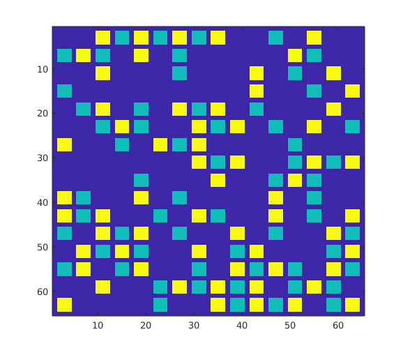


We are interested in the construction of fast numerical solution of the equation (2.4) with coefficients , generated in the course of stochastic realizations. In this problem setting the bottleneck task is fast generation of the (large) FEM stiffness matrix in a sparse format, see [22], which should be re-calculated many thousands times for long sequences of stochastic realizations. Here the computational challenges are twofold:
- (A)
Fine -grids required for the resolution of coefficients on large lattice.
- (B)
Large number of stochastic realizations of the order of that are necessary for reliable estimation of desired stochastic quantities.
In item (A) the construction of new FEM discretization and then generation of large stiffness matrix in data sparse format is required for every stochastic realization. Item (B) requires the fast iterative solver for the arising linear systems of equations, which should be robust with respect to the main model parameters , , and the random equation coefficients. Our techniques suggest the effective approach for solving both problems (A) and (B).


Figure 2.4 illustrates the configuration of the matrix coefficient visualized for an example of 3D realizations on the lattice, with , The number of inclusions is about .
In what follows, we describe both fast and memory-efficient discretization and solution method for the class of stochastic PDEs specified above, which allows the reliable numerical estimate of the mean (homogenized) constant coefficient in the system (2.4) for for rather large value of RVE and various model parameters at the limit of large , see [14, 15, 22]. This approach also allows to effectively estimate the average solution of the 3D stochastic PDE (2.1) with the given right-hand side by using the precomputed homogenized coefficient matrix.
3 Computational scheme for the stochastic average
3.1 Galerkin FEM discretization scheme
The discretization scheme for the -dimensional problem is constructed by FEM on tensor grid in similar to the 2D case described in [22]. We consider the RVE approximation specified by the checkerboard-type realizations of the random coefficient field on the tensor product lattice11 1 That is lattice for , and lattice for .. This lattice is composed of unit cells such that
In 2D case the FEM discretization and the construction of the Galerkin matrix can be viewed as a special case of the more general scheme in [22] based on the “overlapping” type random realizations of the coefficient field.
Given the number with , of the grid intervals specifying the size a unit cell, we introduce the uniform rectangular grid in with the grid size , such that , i.e., . We assume that the “unit cell” , , includes the square “unit sub-cell” of size (that is for ) which adjusts the square grid , such that the center of is located at the center of . The sub-cell denotes the region where the stochastic realization is allowed to generate the jumping coefficient. The number of unit cells where the coefficient is perturbed varies for different stochastic realizations. The overlap factor may take values depending on the choice of . In this construction the univariate size of the unit sub-cell varies as
In the presented numerical examples we normally use the overlap constant or . For , the maximal size of the unit sub-cell is given by , which contains grid points in each spacial direction leading to rectangular grid with .
Fixed , the FEM discretization of the elliptic PDE in (2.2) can be constructed, in general, on a sequence of dyadic refined grids by choosing , so that the increase of the parameter improves the accuracy of FEM approximation.
Given a finite dimensional space of tensor product piecewise linear finite elements associated with the grid , with , , incorporating periodic boundary conditions, we are looking for the traditional FEM Galerkin approximation of the exact solution in the form
where denotes the unknown coefficients vector. Fixed realization of the coefficient , we define the Galerkin-FEM discretization in of the variational formulation of equation (2.2) by
| (3.1) |
where the Galerkin-FEM stiffness matrix generated by the equation coefficient is calculated by using the associated bilinear form
| (3.2) |
and .
In specific application to numerical estimation of the homogenized coefficient matrix the corresponding right-hand side is defined
| (3.3) |
Corresponding to (2.3) and (3.2), we represent the stiffness matrix in the additive form
| (3.4) |
where represents the FEM Laplacian matrix in periodic setting that has the standard -term Kronecker product form. Here matrix provides the FEM approximation to the ”stochastic part” in the elliptic operator corresponding to the coefficient , see (2.3). The latter is determined by the sequence of random coefficient distributions in the course of stochastic realizations, numbered by .
In the case of complicated jumping coefficients the stiffness matrix generation in the elliptic FEM usually constitutes the dominating part of the overall solution cost. The asymptotic convergence of the stochastic homogenization process presupposes that the equation (3.1) has to be solved many hundred or even thousand times, so that for every realization one has to update the stiffness matrix and the right-hand side .
Our discretization scheme computes all matrix entries at a low cost by assembling the local Kronecker products of sparse matrices obtained by representation of as a sum of separable functions. This allows to store the resultant stiffness matrix in the sparse matrix format. Such a construction only includes the pre-computing of small tri-diagonal matrices representing 1D elliptic operators with jumping coefficients in periodic setting. In the following sections, we shall describe the efficient construction of the ”stochastic” term to be updated for every realization.
3.2 Matrix generation by using Kronecker product sums
To enhance the time consuming matrix assembling process we apply the FEM Galerkin discretization (3.2) of equation (2.2) by means of the tensor-product piecewise linear finite elements
for where are the univariate piecewise linear hat functions. Notice that the univariate grid size is of the order of , where the small homogenization parameter is given by , designating the total problem size
The stiffness matrix is constructed by the standard mapping of the multi-index into the long univariate index for the active degrees of freedom in periodic setting. For instance, we use the so-called big-endian convention for and
respectively. We first consider the case in more detail.
We calculate the stiffness matrix by assembling of the local Kronecker product terms by using representation of the “stochastic part” in the coefficient as an -term sum of separable functions. This leads to the linear system of equations
| (3.5) |
constructed for the general -term separable coefficient with .
By simple algebraic transformations (e.g. by lamping of the mass matrices) the matrix can be represented in the form (without loss of approximation order)
| (3.6) |
where are the diagonal matrices with positive entries, and means the Kronecker product of matrices, see the discussion in [22]. This representation applies, in particular, to the periodic Laplacian. For example, in the case of anisotropic Laplacian the representation in (3.6) can be further simplified to
which will be used as a prototype preconditioner for solving the target linear system (3.5).
Taking into account the rectangular structure of the grid, we use the simple finite-difference (FD) scheme for the matrix representation of the Laplacian operator . The scaled discrete Laplacian incorporating periodic boundary conditions takes the form
| (3.7) |
where, say, in the variable we have
such that the entries of the ”periodization” matrix are all zeros except
see (3.8), right. Here is the identity matrix, and are the 1D finite difference Laplacians in variables and , respectively (endorsed with the Neumann boundary conditions). We say that the Kronecker rank of the matrix in (3.7) equals to , .
For the assembling of the stiffness we also need the 1D Laplacian with Neumann boundary conditions. To that end we notice that the Laplacian matrices for the Neumann and periodic boundary conditions in the first 1D variable read as
| (3.8) |
respectively.
In the -dimensional setting we have the similar Kronecker rank- representations. For example, in the case the ”periodic” Laplacian matrix takes a form
| (3.9) |
such that its Kronecker rank equals to , while for the arbitrary , we have .
3.3 Fast matrix assembling for the stochastic part
The Kronecker form representation of the ”stochastic” term in (3.2) further denoted by is more involved. For the ease of exposition we, first, discuss the case , and assume that .
For given stochastically chosen distribution of non-overlapping cells , , where the constant coefficient is perturbed, we introduce the full covered grid domain colored by black in Figure 2.1 and 5.1. We obtain a union of non-overlapping “covered” square cells , , , each of the grid-size ,
| (3.10) |
where the number varies for different realizations. By construction, we have for and for . Here , for some , is fixed as above by the chosen overlap constant , see §3.1. In this construction, the non-overlapping elementary cells for different are allowed to have the only common edges of size .
Notice that in the case of non-overlapping decomposition (3.10) the set of cells may coincide with the initial set that allows to maximize the size of each , , to the largest possible, i.e. to . We refer to [22] for the construction in the case of general overlapping coefficients.
To finalize the matrix generation procedure for , we define the local matrices representing the discrete Laplacian with Neumann boundary conditions,
and the diagonal matrix
see the visualization in (3.8), left. Here, we may select that corresponds to the choice . In the case of matrix with minimal size , both discrete Laplacians in (3.8) simplify to
| (3.11) |
Let the subdomain be supported by the index set of size for . Introduce the block-diagonal matrices and by inserting matrices and , defined above, as diagonal blocks into zero matrix in the positions and , respectively. Now the stiffness matrix is represented in the form of a Kronecker product sum as follows,
| (3.12) |
where
is the ”periodization” matrix in 2D.
In a -dimensional case the representation (3.12) generalizes to a sum of -factor Kronecker products
| (3.13) |
where is the ”periodization” matrix in dimensions, constructed as the -term Kronecker sum similar to the case .
The Kronecker product form of (3.12) and (3.13) leads to the corresponding Kronecker sum representation for the total stiffness matrix . This allows an efficient implementation of the matrix assembly and low storage request for the stiffness matrix preserving the Kronecker sparsity. In general, for 2D case the number of elementary cells22 2 For example, for cells of minimal size, with , as in (3.11), we have . does not exceed , and it may coincides with only in the case of non-overlapping decomposition with maximal size , where different patches are allowed to have joint pieces of boundary, but no overlapping area.
The technical assumption that all sub-cells are supposed to be cell-centered is not essential for the presented construction. The approach also applies to the case of general location of inside of the corresponding unit cell .
For the above constructions, which apply to any dimension , we are able to prove the following storage complexity and Kronecker rank estimates for the stiffness matrix .
Lemma 3.1
The storage size for the stiffness matrix is bounded by
In the general case the Kronecker rank of the matrix is bounded by
In the case of cell-centered locations of subdomains (special case of geometric homogenization) there holds
Proof. The first two estimates directly follow from the construction. To justify the improved rank estimate in 2D case we notice that the -term sum in (3.12) can be simplified as follows. Introduce the horizontal grid strips , , each of width and agglomerate all the summands in (3.12) with into one matrix . It can be seen that . Hence the equation
proves the result for . The rank estimate in the case can be derived completely similar.
The discretized equation (2.2) takes a form
| (3.14) |
where the FEM-Galerkin matrix generated by the equation coefficient is calculated as described above (see [22] for the case of overlapping decompositions).
Notice that in application to RVE approximation of the homogenized matrix one has to solve linear systems of equations with different right-hand sides. The corresponding vector representation , , of the right-hand side is computed by scalar multiplication of with the corresponding Galerkin basis function and integration by parts, see (3.3).
Specifically, given the grid-point , the corresponding value of the diagonal coefficient is defined by , see (2.3). In case the variable part , describing the jumping coefficient, is assigned by for interior points in , by for interface points (the angle equals to ), and by for the ”exterior” corner of (the angle equals to ), see points (d), (b), (c) and (a) in Figure 3.1 (left), respectively. Figure 3.1 (left) corresponds to , the discretization parameter and the periodic completion of the geometry.
The corresponding illustration for the 3D case is presented in Figure 3.1 (right). In case of large number of representative volume elements, , one observes the complicated interface defining the strongly jumping coefficients.
3.4 The RVE approximation of homogenized matrix
For given size of the RVE, , we consider the sequence of problems for stochastic realizations specifying the variable part in the coefficient matrix , ,
| (3.15) |
for .
Fixed and the particular realization , the averaged coefficient matrix , , with the constant entries is conventionally defined by the equation
| (3.16) |
which implies the representation for matrix elements
The latter leads to the entry-wise representation of the homogenized matrix , ,
| (3.17) |
The representation (3.4) ensures the symmetry of the homogenized matrix , i.e. , taking into account the equations (2.4), see [22], §4.2, for the detailed argument.
In numerical implementation, we apply the same variational scheme for calculation (by numerical integration) of as for the FEM discretization of the operator and the right-hand side in the initial elliptic PDE, thus preserving the symmetry of the matrix inherited from the initial variational formulation.
Furthermore, integrals over in (3.4), as they are written for the exact matrix entries , , are calculated (approximately) by using the discrete representation of integrand on the grid .
4 Construction of preconditioner for PCG iteration
4.1 Spectral equivalent preconditioner
Let the right-hand side in (2.1) satisfy , then for a fixed realization , the equation
| (4.1) |
where is the periodic Laplacian, has the unique solution. We solve this equation by the preconditioned conjugate gradient (PCG) iteration with the preconditioner obtained as inverse of the (perturbed) periodic Laplacain
where is the identity matrix and is a small regularization parameter introduced for stability reasons in the case of direct inversion of (that is too costly in 3D case). In what follows, for 3D case, we set up and use the explicit low Kronecker rank approximation of the pseudo-inverse matrix as the preconditioner for solving the algebraic system of equations (4.1) on the subspace . Notice that by the conventional definition we have for all such that , while . Since the pre-factor does not effect the condition number of the preconditioned matrix, in the following discussion we set up it as .
It can be proven that the condition number of preconditioned matrix is uniformly bounded in and . The following Lemma proves the spectral equivalence of the preconditioner, see also [22].
Lemma 4.1
Given the matrix with , then for any stochastic realization the condition number of the preconditioned matrix on the kernel of the stiffness matrix , , is uniformly bounded in , and , such that
Proof. The particular bound on the condition number in terms of a parameter can be derived by introducing the average coefficient
where and are chosen as majorants and minorants of in (2.3), respectively. Indeed, the preconditioner generated by the coefficient allows the condition number estimate
on the subspace . With the choice , the preconditioner corresponds to and , hence, we obtain and the result follows.
The PCG solver for the system of equations (3.14) with the pseudo-inverse of the discrete Laplacian as the preconditioner demonstrates robust convergence with the rate almost uniformly in the model and discretization parameters and the grid size .
Recall that the periodic Laplacian obeys the Kronecker rank- representation, that is the -level circulant matrix, and, hence, it can be diagonalized by the Fourier transform. In particular, in the 2D case the periodic Laplacian takes form (3.7). In the case , the ”periodic” Laplacian matrix is the three-term Kronecker sum (3.9) and similar for the -term representation in the general case .
In the rest of this section, we discuss the main details of our reconditioned PCG scheme for periodic setting that relies on the low Kronecker rank approximation of the pseudo-inverse matrix . In this scheme the CG iteration applies to the preconditioned system of equations in (4.1) as follows
| (4.2) |
that is solved on the subspace due to periodic setting.
4.2 Low Kronecker rank approximation of the preconditioner
The rank-structured preconditioner presented here for periodic setting is obtained by a modification of the construction described in [17] for the Dirichlet boundary conditions, see also [32] where the case of anisotropic Laplacian is considered.
In the periodic setting, the matrix can be diagonalized in the -dimensional Fourier basis, which implies the factorization (for example, in 2D case)
| (4.3) |
with the diagonal matrix
Furthermore, in 3D case we have
| (4.4) |
with the diagonal matrix given by
| (4.5) |
Here the diagonal matrices , , are defined by the Fourier transform of the first column vector
in the circulant matrix in (3.8), diagonalized by the Fourier transform
| (4.6) |
Here , , denote the eigenvalues of the periodic Laplacian , such that . The latter property introduces the significant difference between the periodic case and the case of Dirichlet boundary conditions considered in [17].
The representations (4.3) and (4.4) give rise to the eigenvalue decomposition of . Therefore, for a function applied to the matrix , we arrive at
| (4.7) |
and
| (4.8) |
for 2D and 3D cases, respectively. In our application we have to approximate the diagonal matrix in the case of periodic Laplacian, where has zero eigenvalue.
To construct the efficient preconditioner for the system matrix , we are particularly interested in the low Kronecker rank approximation of the pseudo-inverse matrix that provides the spectrally close approximation to . Since in the case of periodic boundary conditions the matrix has zero eigenvalue corresponding to the constant vector, one has to consider the pseudo-inverse matrix instead of the standard inverse that means the matrix should be defined by setting the first element in to zero.
We discuss two different solution strategies for multiple solving the target algebraic system of linear equations in (4.1).
The first approach is based on the FFT diagonalization of pseudo-inverse preconditioning matrix by using the pseudo-inverse . In this case the system matrix is stored in the standard sparse matrix format and the PCG solution process is performed in the exact matrix arithmetics.
In the second approach, we represent both the system matrix and preconditioner in the low Kronecker rank form and store both large matrices and as a small set of thin Kronecker factor matrices which allows to implement the PCG iteration on the low parametric manifold of low-rank discretized functions.
Here we briefly discuss the second approach. In the 3D case, the elements of the core diagonal matrix in (4.5) can be represented as a three-tensor
where
implying that has the exact rank- decomposition. Here the periodicity conditions imply such that . In the case we have the two-term sum representation, . We further set .
In the 3D case we consider the low-rank decomposition of the reciprocal core tensor obtained by folding of the pseudo-inverse matrix ,
| (4.9) |
with entries defined for , by plugging zero value in the element , and leaving the rest of the elements in the reciprocal tensor unchanged,
| (4.10) |
The theory on the low-rank tensor approximation of the target tensor is based on the integral Laplace transform representation of the discrete function for
| (4.11) |
under the conditions
| (4.12) |
which is satisfied for our construction.
Given , under the condition (4.12) there exist the rank- canonical -approximation of the tensor with , see for example [24] for more details. Then we split the target tensor into the sum
where
while
Now applying the result for tensors of the type to each of components separately we easily obtain the rank bounds
thus implying the desired upper bound on the canonical rank
This argument proves the following
Lemma 4.2
Given , under the condition (4.12) there exist the rank- canonical -approximation of the tensor . The target tensor can be approximated by a rank canonical decomposition with accuracy , where .
From the algorithmic point of view, the rank-structured approximation to the discrete periodic Laplacian inverse operators is performed by using the multigrid Tucker decomposition of the 3D tensors obtained by reshaping of the diagonal system matrix represented in the Fourier basis into a 3D tensor . The subsequent Tucker-to-canonical decomposition, see [23], transforms the Tucker core tensor to a canonical one with a small rank, preserving the approximation precision of the Tucker decomposition.
Now assume that can be expressed approximately by a short-term linear combination of Kronecker rank- matrices. Then, the low-rank approximation of is reduced to approximation of the diagonal matrix . Assume we have a decomposition (in 2D case)
with vectors and . Now let be a vector given in a low-rank format, i.e.
with vectors and . Then a matrix-vector product can be calculated by using only 1D matrix-vector operations
| (4.13) |
where denotes the componentwise (Hadamard) product of 1D vectors. Using the FFT, the expression (4.13) can be computed in factored form in flops, where .
In the case , equation (4.13) takes a form
| (4.14) |
and similar in the general case of . Notice that the total number of terms in (4.14), that is , does not depend on the number of dimensions .
The numerical performance of the PCG iteration with the rank-structured preconditioner described above will be discussed in section 5.
5 Numerical study
5.1 Fast solvers using matrix generation combined with tensor-product preconditioner
Here, we consider the beneficial properties of the presented elliptic problem solver applied to the case of checkerboard type coefficients profile compared with the previous scheme with more general overlapping-type configurations [22]. Figure 5.1 illustrates the configuration of the stochastic realization for checkerboard type coefficient with large RVE size, .


Table 5.1 compares the CPU times (sec.) for matrix generation, calculation of the loading vector in the right-hand side, and for the PCG iteration in the course of solving equation (4.1) for the general case of overlapping-type realizations of coefficients considered in [22] (marked by (1)), and for the approach presented in this paper and based on the low-rank preconditioner (marked by (2)). Here we set , (see Figure 5.1, top), such that the vector size on the finest grid is about . The iteration stopping criteria is chosen by .
| / | matr. (1) | matr. (2) | RHS (1) | RHS (2) | solve (1) | solve (2) | |
| 17/289 | 0.012 | 0.006 | 0.01 | 0.007 | 0.006 | 0.01 | |
| 33/1089 | 0.06 | 0.007 | 0.045 | 0.003 | 0.137 | 0.027 | |
| 65/4225 | 0.34 | 0.014 | 0.19 | 0.010 | 0.11 | 0.15 | |
| 129/16641 | 3.0 | 0.038 | 0.8 | 0.014 | 0.5 | 0.6 | |
| 257/66049 | 36 | 0.24 | 3.7 | 0.069 | 2.6 | 2.2 | |
| 513/263169 | 561 | 1.4 | 22 | 0.38 | 13.8 | 11.9 | |
| 1025/ | – | 11.3 | – | 2.84 | – | 66.8 | |
| 2049/ | – | 105.6 | – | 1.2 | – | 360.0 |
Solver (1) corresponding to overlapping coefficients profile displays limitations in the matrix generation times (dominating part in the calculations) for , which exceeds seconds. Matrix generation time for the solver (2) using checkerboard-type coefficient is essentially smaller ( seconds), which is important taking into account the required large number of realizations (up to ) to be performed for analyzing important quantities of stochastic problem in random media. For larger the solver (2) might be limited by the solution time, which is about seconds for .
The latter limitation can be relaxed by using the low Kronecker rank (LKR) preconditioner described in the previous section. In this case we observe the balance between the matrix generation cost and that for the PCG iteration. Table 5.2 represents CPU times (sec.) for PCG iteration with a regularized preconditioner (RP) and with the LKR preconditioner by using the rank-structured approximation of the pseudo-inverse matrix , both applied with parameters , and tolerance . The number of inclusions varies from to .
| RP | 0.007 | 0.04 | 0.14 | 0.6 | 3.4 | 12.4 | 59.4 | 382.0 |
| LKRP | 0.008 | 0.02 | 0.02 | 0.8 | 0.27 | 0.9 | 6.1 | 11.0 |
Finally we notice that our numerical tests confirm Lemma 4.1 which proves uniform spectral equivalence of the preconditioned in both the grid-size and the RVE size . Indeed, fixed the stopping criteria, the number of PCG iterations was almost the same for numerical experiments in 2D and 3D cases.
5.2 Fast solver for the 3D stochastic problem
Numerical simulations for 3D stochastic homogenization require much larger computational resources compared with 2D case. Notice that fixed , the problem size (i.e., vector size ) in the 3D case for and equals to and , respectively, where . The assembling of the corresponding huge system matrix is performed by fast tensor based techniques as described in section 3.3, see also [22]. The system matrix has to be recomputed for large number of stochastic realizations , that might be of the order of several tens of thousand and more.


Figure 5.2 (left) illustrates the configuration of the matrix coefficient visualized for the 3D realization on the lattice, with , and the density parameter . The number of inclusions is about . Figure 5.2 (right) presents the example of random coefficient with two different values of contrast.
| / | matr. | RHS | solver | |||
| 17/ 4913 | 6.25e-02 | 32 | 0.012 | 0.013 | 0.04 | |
| 33/ 35937 | 3.13e-02 | 238 | 0.02 | 0.015 | 0.13 | |
| 65/ 274625 | 1.56e-02 | 2048 | 0.1 | 0.05 | 0.62 | |
| 129/ 2.1+06 | 7.81e-03 | 16338 | 2.4 | 0.38 | 11.2 | |
| 257/ 16.9e+06 | 3.90e-03 | 131494 | 28.9 | 2.7 | 35.1 | |
| 513/ 135e+06 | 1.95e-03 | 1049066 | 431.7 | 20.6 | 425 |


We demonstrate the computational complexity of the robust iterative solver for 3D elliptic problems applying the stopping criteria . In all cases the number of PCG iterations did not exceed uniformly in the problem size.
Table 5.3 displays the computation times for one solve of the 3D stochastic problem for increasing RVE size of , and respectively increasing vector size in the linear system of equations, as well as the number of stochastic samples, , for the fixed realization For example, the vector size for is about , and the corresponding number of stochastic samples exceeds . This huge problem is solved in about minutes (425 sec) in Matlab. Figure 5.3 (right) visualizes the data presented in Table 5.3.
We point out that the main time consuming steps include the matrix generation and the solution of the discrete elliptic problem for every of three dimensions by calling the “PCG” iteration routine with the rank-structured preconditioner in the form of periodic Laplacian pseudo inverse. We observe the well balanced complexity of both time consuming steps of the algorithms.
5.3 Example of application to numerical estimation of the homogenized coefficient matrix
The set of numerical approximations to the homogenized matrix is calculated by (3.16) for the sequence of realizations, where is large enough, and the artificial period defines the size of RVE. For a fixed , the approximation is computed as the empirical average of the sequence ,
| (5.1) |
By the law of large numbers we have that the empirical average converges almost surely to the ensemble average (expectation)
| (5.2) |
Furthermore, by qualitative homogenization theory, as the artificial period , this converges to the homogenized matrix, see [16],
| (5.3) |
In some cases, we use the entry-wise notation for matrices , , for example, and , etc.
As an example for application of our techniques, we numerically study the asymptotic of the random part of the error (standard deviation) for fixed of moderate size, to confirm the theoretical convergence rate in , see [16],
| (5.4) |
In numerical experiments the theoretical value of standard deviation is approximated by the commonly used computable quantity calculated for a long enough sequence of realizations by
The numerical results are illustrated in Figure 5.4. The calculations for 2D case, depicted in the left panel can be compare with the similar results in [22] obtained for the case of overlapping coefficients sampling. Figure 5.4, right, confirms the asymptotic estimate in (5.4) for 3D case.
6 Conclusions
We present the numerical techniques for discretization and fast solution of the 2D and 3D elliptic equations with strongly varying piecewise constant coefficients arising in numerical analysis of stochastic homogenization problems for multi-scale composite materials. We use random checkerboard coefficient configurations with the large size of the RVE, . For a fixed , our method allows to avoid the generation of the new FEM space at each stochastic realization. For every realization, fast assembling of the FEM stiffness matrix is performed by agglomerating the Kronecker tensor products of 1D FEM discretization matrices.
The spectrally close preconditioner is constructed by using the low Kronecker rank approximation to the pseudo-inverse of discrete 2D and 3D periodic Laplacian. The resulting large linear system of equations is solved by the preconditioned CG iteration with the convergence rate that is independent of and the grid size, as well as of the variation in jumping coefficients. The numerical tests illustrate the performance of the Matlab implementation in both 2D and 3D cases.
The proposed elliptic problem solver can be applied in the numerical analysis of 3D stochastic homogenization problems for ergodic processes with variable contrast in random coefficients, for solving numerically the 3D stochastic elliptic PDEs in random heterogeneous materials, for solution of quasi-periodic (multi-scale) geometric homogenization problems, in the computer simulation of dynamical many body interaction processes and multi-particle electrostatics, as well as for numerical analysis of optimal control problems in random media.
Acknowledgements
The authors are thankful to Prof. Felix Otto for useful discussions and motivation to develop an efficient solution scheme for the 3D elliptic PDEs with random coefficients in relation to numerical simulations for stochastic homogenization problems.
References
- [1] G. Allaire. Shape optimization by the homogenization method. Springer Science & Business Media, Band 146, 2012.
- [2] A. Anantharaman, R. Costaouec, C. Le Bris, F. Legoll and F. Thomines. Introduction to numerical stochastic homogenization and the related computational challenges: some recent developments. In Lecture Notes Series, Institute for Mathematical Sciences, Vol. 22, eds. Weizhu Bao and Qiang Du (National University of Singapore), 2011, pp 197–272.
- [3] A. Bensoussan, J.-L. Lions, and G. Papanicolaou. Asymptotic Analysis for Periodic Structures. American Mathematical Society, 1978.
- [4] E. Cances, V. Ehrlacher, F. Legoll, and B. Stamm. An embedded corrector problem to approximate the homogenized coefficients of an elliptic equation. C. R. Acad. Sci. Paris, Série I, 353:801-806, 2015.
- [5] Eric Cances, Virginie Ehrlacher, Frederic Legoll, Benjamin Stamm, Shuyang Xiang. An embedded corrector problem for homogenization. Part I: Theory. E-preprint arXiv:1807.05131, 2018.
- [6] Eric Cances, Virginie Ehrlacher, Frederic Legoll, Benjamin Stamm, Shuyang Xiang. An embedded corrector problem for homogenization. Part II: Algorithms and discretization. arXiv: http://arxiv.org/abs/1810.09885v1, 2018.
- [7] A. Cohen, R. Devore, C. Schwab. Analytic regularity and polynomial approximation of parametric and stochastic elliptic PDE’s. Analysis and Applications 9 (01), 11-47, 2011.
- [8] S. Dolgov, B. N. Khoromskij, A. Litvinenko, H. G. Matthies. Polynomial chaos expansion of random coefficients and the solution of stochastic partial differential equations in the tensor train format. SIAM/ASA Journal on Uncertainty Quantification 3 (1), 1109-1135, 2015.
- [9] S. Dolgov, R. Scheichl. A Hybrid Alternating Least Squares–TT-Cross Algorithm for Parametric PDEs. SIAM/ASA Journal on Uncertainty Quantification 7 (1), 260-291, 2019.
- [10] B. Engquist and P.E. Souganidis. Asymptotic and numerical homogenization. Acta Numerica,17:147–190, 2008.
- [11] Julian Fischer. The choice of representative volumes in the approximation of the effective properties of random materials. E-preprint, arXiv:1807.00834, 2018.
- [12] P. Frauenfelder, C. Schwab, R. A. Todor. Finite elements for elliptic problems with stochastic coefficients. Computer methods in applied mechanics and engineering 194 (2-5), 205-228, 2005.
- [13] A. Gloria and F. Otto. An optimal variance estimate in stochastic homogenization of discrete elliptic equations. Ann. Probab., 39:779–856, 2011.
- [14] Antoine Gloria and Felix Otto: An optimal error estimate in stochastic homogenization of discrete elliptic equations. In: The annals of applied probability, 22 (2012) 1, p. 1-28.
- [15] Antoine Gloria and Felix Otto. The corrector in stochastic homogenization: near-optimal rates with optimal stochastic integrability. arXiv: http://arxiv.org/abs/1510.08290, 2016.
- [16] Antoine Gloria and Felix Otto. Quantitative estimates on the periodic approximation of the corrector in stochastic homogenization In: ESAIM / Proceedings, 48 (2015), p. 80-97. DOI: 10.1051/proc/201448003.
- [17] G. Heidel, V. Khoromskaia, B. Khoromskij, and V. Schulz. Tensor approach to optimal control problems with fractional -dimensional elliptic operator in constraints. E-preprint, arXiv:1809.01971v2, 2018.
- [18] V. Jikov, S. Kozlov, and O. Oleinik. Homogenization of differential operators and integral functionals. Springer, Berlin, 1995.
- [19] T. Kanit, S. Forest, I. Galliet, V. Mounoury and D. Jeulin. Determination of the size of the representative volume element for random composites: statistical and numerical approach. Int. J. of Solids and Structures, 40, 2003, 3647-3679.
- [20] V. Kazeev, I. Oseledets, M. Rakhuba, C. Schwab. Quantized tensor FEM for multiscale problems: diffusion problems in two and three dimensions. E-preprint arXiv:2006.01455, 2020.
- [21] V. Khoromskaia and B. N. Khoromskij. Tensor numerical methods in quantum chemistry. De Gruyter, Berlin, 2018.
- [22] V. Khoromskaia, B. N. Khoromskij, and F. Otto. Numerical study in stochastic homogenization for elliptic partial differential equations: Convergence rate in the size of representative volume elements. Numer. Lin. Algebra Appl., 27 (3), e2296, 2020.
- [23] B. N. Khoromskij and V. Khoromskaia. Multigrid Tensor Approximation of Function Related Arrays. SIAM J. Sci. Comp., 31(4), 3002-3026 (2009).
- [24] Boris N. Khoromskij. Tensor Numerical Methods in Scientific Computing. Research monograph, De Gruyter Verlag, Berlin, 2018.
- [25] B.N. Khoromskij, and I. Oseledets. Quantics-TT collocation approximation of parameter-dependent and stochastic elliptic PDEs. Comp. Meth. in Applied Math., 10(4):34-365, 2010.
- [26] B.N. Khoromskij, A. Litvinenko, and H.G. Matthies. Application of hierarchical matrices for computing the Karhunen-Loéve expansion. Computing 84: 49-67 (2009).
- [27] B.N. Khoromskij and S. Repin. Rank structured approximation method for quasi–periodic elliptic problems. Comput. Methods in Appl. Math. 2017; 17 (3):457-477.
- [28] B. N. Khoromskij and Ch. Schwab. Tensor-structured Galerkin approximation of parametric and stochastic elliptic PDEs. SIAM J. Sci. Comput. 33 (1), 364-385, 2011.
- [29] S.M. Kozlov. Averaging of random operators. Matematicheskii Sbornik, 151(2):188-202, 1979.
- [30] F. Y. Kuo, C. Schwab, I. H. Sloan. Quasi-Monte Carlo finite element methods for a class of elliptic partial differential equations with random coefficients. SIAM Journal on Numerical Analysis 50 (6), 3351-3374, 2012.
- [31] C. Le Bris and F. Legoll. Examples of computational approaches for elliptic possibly multiscale PDEs with random inputs. J Comp. Phys., 328 (2017) 455-473.
- [32] B. Schmitt, B. Khoromskij, V. Khoromskaia, and V. Schulz. Tensor Method for Optimal Control Problems Constrained by Fractional 3D Elliptic Operator with Variable Coefficients. E-preprint, arXiv:2006.09314, 2020.
- [33] C. Schwab, C. J. Gittelson. Sparse tensor discretizations of high-dimensional parametric and stochastic PDEs. Acta Numerica 20, 291-467, 2011.