Efficient Optimistic Exploration in Linear-Quadratic Regulators
via Lagrangian Relaxation

Marc Abeille Affiliation: Criteo AI Lab Correspondence to: m.abeille@criteo.com Alessandro Lazaric Affiliation: Facebook AI Research

Abstract

We study the exploration-exploitation dilemma in the linear quadratic regulator (LQR) setting. Inspired by the extended value iteration algorithm used in optimistic algorithms for finite MDPs, we propose to relax the optimistic optimization of OFU-LQ and cast it into a constrained extended LQR problem, where an additional control variable implicitly selects the system dynamics within a confidence interval. We then move to the corresponding Lagrangian formulation for which we prove strong duality. As a result, we show that an $\epsilon$ -optimistic controller can be computed efficiently by solving at most $O\big(\log(1/\epsilon)\big)$ Riccati equations. Finally, we prove that relaxing the original OFU problem does not impact the learning performance, thus recovering the $\widetilde{O}(\sqrt{T})$ regret of OFU-LQ. To the best of our knowledge, this is the first computationally efficient confidence-based algorithm for LQR with worst-case optimal regret guarantees.

Keywords:

LQR, Optimism, exploration, reinforcement learning

1 Introduction

Exploration-exploitation in Markov decision processes (MDPs) with continuous state-action spaces is a challenging problem: estimating the parameters of a generic MDP may require many samples, and computing the corresponding optimal policy may be computationally prohibitive. The linear quadratic regulator (LQR) model formalizes continuous state-action problems, where the dynamics is linear and the cost is quadratic in state and action variables. Thanks to its specific structure, it is possible to efficiently estimate the parameters of the LQR by least-squares regression and the optimal policy can be computed by solving a Riccati equation. As a result, several exploration strategies have been adapted to the LQR to obtain effective learning algorithms.

Confidence-based exploration. Bittanti et al. 2006 introduced an adaptive control system based on the “bet on best” principle and proved asymptotic performance guarantees showing that their method would eventually converge to the optimal control. Abbasi-Yadkori & Szepesvári 2011 later proved a finite-time $\widetilde{O}(\sqrt{T})$ regret bound for OFU-LQ, later generalized to less restrictive stabilization and noise assumptions by Faradonbeh et al. 2017. Unfortunately, neither exploration strategy comes with a computationally efficient algorithm to solve the optimistic LQR, and thus they cannot be directly implemented. On the TS side, Ouyang et al. 2017 proved a $\widetilde{O}(\sqrt{T})$ regret for the Bayesian regret, while Abeille & Lazaric 2018 showed that a similar bound holds in the frequentist case but restricted to 1-dimensional problems. While TS-based approaches require solving a single (random) LQR, the theoretical analysis of Abeille & Lazaric 2018 suggests that a new LQR instance should be solved at each time step, thus leading to a computational complexity growing linearly with the total number of steps. On the other hand, OFU-based methods allow for “lazy” updates, which require solving an optimistic LQR only a logarithmic number of times w.r.t. the total number of steps. A similar lazy-update scheme is used by Dean et al. 2018, who leveraged robust control theory to devise the first learning algorithm with polynomial complexity and sublinear regret. Nonetheless, the resulting adaptive algorithm suffers from a $\widetilde{O}(T^{2/3})$ regret, which is significantly worse than the $\widetilde{O}(\sqrt{T})$ achieved by OFU-LQ.

To the best of our knowledge, the only efficient algorithm for confidence-based exploration with $\widetilde{O}(\sqrt{T})$ regret has been recently proposed by Cohen et al. 2019. Their method, called OSLO, leverages an SDP formulation of the LQ problem, where an optimistic version of the constraints is used. As such, it translates the original non-convex OFU-LQ optimization problem into a convex SDP. While solving an SDP is known to have polynomial complexity, no explicit analysis is provided and it is said that the runtime may scale polynomially with LQ-specific parameters and the time horizon $T$ (Cor. 5), suggesting that OSLO may become impractical for moderately large $T$ . Furthermore, OSLO requires an initial system identification phase of length $\widetilde{O}(\sqrt{T})$ to properly initialize the method. This strong requirement effectively reduces OSLO to an explore-then-commit strategy, whose regret is dominated by the length of the initial phase.

Perturbed certainty equivalence exploration. A recent stream of research (Faradonbeh et al. 2018b; Mania et al. 2019; Simchowitz & Foster 2020) studies variants of the perturbed certainty equivalence (CE) controller (i.e., the optimal controller for the estimated LQR) and showed that this simple exploration strategy is sufficient to reach worst-case optimal regret $\widetilde{O}(\sqrt{T})$ . Since the CE controller is not recomputed at each step (i.e., lazy updates) and the perturbation is obtained by sampling from a Gaussian distribution, the resulting methods are computationally efficient. Nonetheless, these methods rely on an isotropic perturbation (i.e., all control dimensions are equally perturbed) and they require the variance to be large enough so as to eventually reduce the uncertainty on the system estimate along the dimensions that are not naturally “excited” by the CE controller and the environment noise. Being agnostic to the uncertainty of the model estimate and its impact on the average cost, may lead this type of approaches to have longer (unnecessary) exploration and larger regret. On the other hand, confidence-based methods relies on exploration controllers that are explicitly designed to excite more the dimensions with higher uncertainty and impact on the performance. As a result, they are able to perform more effective exploration. We further discuss this difference in Sect. 6.

In this paper, we introduce a novel instance of OFU, for which we derive a computationally efficient algorithm to solve the optimistic LQR with explicit computational complexity and $\widetilde{O}(\sqrt{T})$ regret guarantees. Our approach is inspired by the extended value iteration (EVI) used to solve a similar optimistic optimization problem in finite state-action MDPs (Jaksch et al. 2010, e.g.). Relying on an initial estimate of the system obtained after a finite number of system identification steps, we first relax the confidence ellipsoid constraints and we cast the OFU optimization problem into a constrained LQR with extended control. We show that the relaxation of the confidence ellipsoid constraint does not impact the regret and we recover a $\widetilde{O}(\sqrt{T})$ bound. We then turn the constrained LQR into a regularized optimization problem via Lagrangian relaxation. We prove strong duality and show that we can compute an $\epsilon$ -optimistic and $\epsilon$ -feasible solution for the constrained LQR by solving only $O(\log(1/\epsilon))$ algebraic Riccati equations. As a result, we obtain the first efficient worst-case optimal confidence-based algorithm for LQR. In deriving these results, we introduce a novel derivation of explicit conditions on the accuracy of the system identification phase leveraging tools from Lyapunov stability theory that may be of independent interest.

2 Preliminaries

We consider the discrete-time linear quadratic regulator (LQR) problem. At any time $t$ , given state $x_{t}\in\mathbb{R}^{n}$ and control $u_{t}\in\mathbb{R}^{d}$ , the next state and cost are obtained as

	$\displaystyle x_{t+1}$	$\displaystyle=A_{}x_{t}+B_{}u_{t}+\epsilon_{t+1};$		(1)
	$\displaystyle c(x_{t},u_{t})$	$\displaystyle=x_{t}^{\mathsf{T}}Qx_{t}+u_{t}^{\mathsf{T}}Ru_{t},$		(1)

where $A_{*}$ , $B_{*}$ , $Q$ , $R$ are matrices of appropriate dimension and $\{\epsilon_{t+1}\}_{t}$ is the process noise. Let $\mathcal{F}_{t}=\sigma(x_{0},u_{0},\dots,x_{t},u_{t})$ be the filtration up to time $t$ , we rely on the following assumption on the noise.¹¹ 1 As shown by Faradonbeh et al. 2017, this can be relaxed to Weibull distributions with known covariance.

Assumption 1.

The noise $\{\epsilon_{t}\}_{t}$ is a martingale difference sequence w.r.t. the filtration $\mathcal{F}_{t}$ and it is componentwise conditionally sub-Gaussian, i.e., there exists $\sigma>0$ such that $\mathbb{E}(\exp(\gamma\epsilon_{t+1,i})|\mathcal{F}_{t})\leq\exp(\gamma^{2}\sigma^{2}/2)$ for all $\gamma\in\mathbb{R}$ . Furthermore, we assume that the covariance of $\epsilon_{t}$ is the identity matrix.

The dynamics parameters are summarized in $\theta_{*}^{\mathsf{T}}=(A_{*},B_{*})$ and the cost function can be written as $c(x_{t},u_{t})=z_{t}^{\mathsf{T}}Cz_{t}$ with $z_{t}=(x_{t},u_{t})^{\mathsf{T}}$ and the cost matrix

C=\begin{pmatrix}Q&0\\ 0&R\end{pmatrix}.

(2)

The solution to an LQ is a stationary deterministic policy $\pi:\mathbb{R}^{n}\rightarrow\mathbb{R}^{d}$ mapping states to controls minimizing the infinite-horizon average expected cost

J_{\pi}(\theta_{*})=\limsup_{T\rightarrow\infty}\frac{1}{T}\mathbb{E}\bigg[\sum_{t=0}^{T}c(x_{t},u_{t})\bigg],

(3)

with $x_{0}=0$ and $u_{t}=\pi(x_{t})$ . We assume that the LQR problem is “well-posed”.

Assumption 2.

The cost matrices $Q$ and $R$ are symmetric p.d. and known, and $(A_{*},B_{*})$ is stabilizable, i.e., there exists a controller $K$ , such that $\rho(A_{*}+B_{*}K)<1$ .²² 2 $\rho(A)$ is the spectral radius of the matrix $A$ , i.e., the largest absolute value of the eigenvalues of $A$ .

In this case, Thm.16.6.4 in (Lancaster & Rodman 1995) guarantees the existence and uniqueness of an optimal policy $\pi_{*}=\arg\min_{\pi}J_{\pi}(\theta_{*})$ , which is linear in the state, i.e., $\pi_{*}(x)=K(\theta_{*})x$ , where,

	$\displaystyle K(\theta_{*})$	$\displaystyle=-\big(R+B_{}^{\mathsf{T}}P(\theta_{})B_{}\big)^{-1}B_{}^{\mathsf{T}}P(\theta_{})A_{},$		(4)
	$\displaystyle P(\theta_{*})$	$\displaystyle=Q+A_{}^{\mathsf{T}}P(\theta_{})A_{}+A_{}^{\mathsf{T}}P(\theta_{})B_{}K(\theta_{*}).$		(4)

For convenience, we will denote $P_{*}=P(\theta_{*})$ . The optimal average cost is $J_{*}=J_{\pi_{*}}(\theta_{*})=\text{Tr}(P_{*})$ . Further, let $L(\theta_{*})^{\mathsf{T}}=\big(I\;K(\theta_{*})^{\mathsf{T}}\big)$ , then the closed-loop matrix $A^{\mathsf{c}}(\theta_{*})=A_{*}+B_{*}K(\theta_{*})=\theta_{*}^{\mathsf{T}}L(\theta_{*})$ is asymptotically stable.

While Asm. 2 guarantees the existence of an optimal linear controller, its optimal cost $J_{*}$ may still grow unbounded when $\theta_{*}$ is nearly unstable. A popular solution is to introduce a “strong” stability assumption (i.e., $\rho(A^{\mathsf{c}}(\theta_{*}))\leq\overline{\rho}<1$ ). Nonetheless, this imposes stability uniformly over all state dimensions, whereas, depending on the cost matrices $Q$ and $R$ , some dimensions may be less sensitive than others in terms of their impact on the cost. Here we prefer imposing an assumption directly on the optimal cost.³³ 3 An alternative assumption may bound the operator norm of $P_{*}$ , (see e.g., Simchowitz & Foster 2020).

Assumption 3.

There exists $D>0$ such that $J_{*}=\text{Tr}(P_{*})\leq D$ and $D$ is known.

Finally, we introduce $\kappa=D/\lambda_{\min}(C)$ , a quantity that will characterize the complexity of many aspects of the learning problem in the following. Intuitively, $\kappa$ measures the cost of controlling w.r.t. the minimum cost incurred if the uncontrolled system was perfectly stable.

The learning problem. We assume that $Q$ and $R$ are known, while $\theta_{*}$ needs to be estimated from data. We consider the online learning problem where at each step $t$ the learner observes the current state $x_{t}$ , it executes a control $u_{t}$ and it incurs the associated cost $c(x_{t},u_{t})$ ; the system then transitions to the next state $x_{t+1}$ according to Eq. 1. The learning performance is measured by the cumulative regret over $T$ steps defined as $\mathcal{R}_{T}(\theta_{*})=\sum_{t=0}^{T}\big(c_{t}-J_{*}(\theta_{*})\big).$ Exploiting the linearity of the dynamics, the unknown parameter $\theta_{*}$ can be directly estimated from data by regularized least-squares (RLS). For any sequence of controls $(u_{0},\ldots,u_{t})$ and the induced states $(x_{0},x_{1},\ldots,x_{t+1})$ , let $z_{t}=(x_{t},u_{t})^{\mathsf{T}}$ , the RLS estimator with a regularization bias $\theta_{0}$ and regularization parameter $\lambda\in\mathbb{R}_{+}^{*}$ defined as⁴⁴ 4 For $\theta_{0}=0$ , this reduces to the standard estimator. The need for a “centered” regularization term is explained in the next section.

	$\displaystyle\widehat{\theta}_{t}$	$\displaystyle=\argmin_{\theta\in\mathbb{R}^{(n+d)\times n}}\sum_{s=0}^{t-1}\\|x_{s+1}-\theta^{\mathsf{T}}z_{s}\\|^{2}+\lambda\\|\theta-\theta_{0}\\|^{2}_{F}$		(5)
		$\displaystyle=V_{t}^{-1}\Big(\lambda\theta_{0}+\sum_{s=0}^{t-1}z_{s}x_{s+1}^{\mathsf{T}}\Big),$		(5)

where $V_{t}=\lambda I+\sum_{s=0}^{t-1}z_{s}z_{s}^{\mathsf{T}}$ is the design matrix. The RLS estimator concentrates as follows (see section C.3).

Proposition 1 (Thm. 1 in Abbasi-Yadkori & Szepesvári 2011).

For any $\delta\in(0,1)$ and any $\mathcal{F}_{t}$ -adapted sequence $(z_{0},\ldots,z_{t})$ , the RLS estimator $\hat{\theta}_{t}$ is such that

		$\displaystyle\\|\theta_{*}-\widehat{\theta}_{t}\\|_{V_{t}}\leq\beta_{t}(\delta)\quad\quad\text{where}$		(6)
		$\displaystyle\beta_{t}(\delta)=\sigma\sqrt{2n\log\Big(\frac{\det(V_{t})^{1/2}n}{\det(\lambda I)^{1/2}\delta}\Big)}+\lambda^{1/2}\\|\theta_{0}-\theta_{*}\\|_{F},$

w.p. $1-\delta$ (w.r.t. the noise $\{\epsilon_{t+1}\}_{t}$ and any randomization in the choice of the control).

Finally, we recall a standard result of RLS.

Proposition 2 (Lem. 10 in Abbasi-Yadkori & Szepesvári 2011).

Let $\lambda\geq 1$ , for any arbitrary $\mathcal{F}_{t}$ -adapted sequence $(z_{0},z_{1},\ldots,z_{t})$ , let $V_{t+1}$ be the corresponding design matrix, then

\sum_{s=0}^{t}\min\big(\|z_{s}\|_{V_{s}^{-1}}^{2},1\big)\leq 2\log\frac{\det(V_{t+1})}{\det(\lambda I)}.

Moreover when $\|z_{t}\|\leq Z$ for all $t\geq 0$ , then

\sum_{s=0}^{t}\|z_{s}\|_{V_{s}^{-1}}^{2}\leq\left(\!1\!+\!\frac{Z^{2}}{\lambda}\!\right)(n\!+\!d)\log\Big(1+\frac{(t\!+\!1)Z^{2}}{\lambda(n\!+\!d)}\Big).

(7)

3 A Sequentially Stable Variant of OFU-LQ

In this section we introduce a variant of the original OFU-LQ of Abbasi-Yadkori & Szepesvári 2011 that we refer to as OFU-LQ++. Similar to (Faradonbeh et al. 2017), we use an initial system identification phase to initialize the system and we provide explicit conditions on the accuracy required to guarantee sequential stability thereafter. This result is obtained leveraging tools from Lyapunov stability theory which may be of independent interest.

Faradonbeh et al. 2018a showed that it is possible to construct a set $\Theta_{0}=\{\theta:\|\theta-\theta_{0}\|\leq\epsilon_{0}\}$ containing the true parameters $\theta^{*}$ with high probability, through a system identification phase where a randomized sequence of linear controllers is used to accurately estimate the dynamics. In particular, they proved that a set $\Theta_{0}$ with accuracy $\epsilon_{0}$ can be obtained by running the system identification phase for as long as $T_{0}=\Omega(\epsilon_{0}^{-2})$ steps.⁵⁵ 5 An alternative scheme for system identification requires access to a stable controller $K_{0}$ and to perturb the corresponding controls to returned a set $\Theta_{0}$ of desired accuracy $\epsilon_{0}$ (see e.g., Simchowitz & Foster 2020).

After the initial phase, OFU-LQ++ uses the estimate $\theta_{0}$ to regularize the RLS as in (5) and it proceeds through episodes. At the beginning of episode $k$ it computes a parameter

\displaystyle\theta_{k}=\arg\min_{\theta\in\mathcal{C}_{k}}J(\theta),

(8)

where $t_{k}$ is the step at which episode $k$ begins and the constrained set $\mathcal{C}_{k}$ is defined as

\displaystyle\mathcal{C}_{k}=\mathcal{C}(\beta_{t_{k}},V_{t_{k}}):=\{\theta:\|\theta-\widehat{\theta}_{t_{k}}\|_{V_{t_{k}}}\leq\beta_{t_{k}}\},

(9)

where $\beta_{t}=\beta_{t}(\delta/4)$ is defined in (6). Then the corresponding optimal control $K(\theta_{k})$ is computed (4) and the associated policy is executed until $\det(V_{t})\geq 2\det(V_{t_{k}})$ .

Lemma 1.

Let $\Theta_{0}=\{\theta:\|\theta-\theta_{0}\|\leq\epsilon_{0}\}$ be the output of the initial system identification phase of Faradonbeh et al. 2018a. For all $t\geq 0$ , consider the confidence ellipsoid $\mathcal{C}_{t}:=\{\theta:\|\theta-\widehat{\theta}_{t}\|_{V_{t}}\leq\beta_{t}\}$ , where $\widehat{\theta}_{t}$ and $V_{t}$ are defined in eq. 5 with regularization bias $\theta_{0}$ (the center of $\Theta_{0}$ ), regularization parameter

\displaystyle\lambda\!=\!\frac{2n\sigma^{2}}{\epsilon_{0}^{2}}\!\Big(\!\log(4n/\delta)\!+\!(n+d)\!\log\Big(\!1+\!\kappa X^{2}T\Big)\!\Big),

(10)

and $\beta_{t}$ is defined in (6) where $\|\theta-\theta_{*}\|$ is replaced by its upper-bound $\epsilon_{0}$ . Let $\{K(\theta_{t})\}_{t\geq 1}$ be the sequence of optimistic controllers generated by OFU-LQ++ and let $\{x_{t}\}_{t\geq 0}$ be the induced state process (Eq. 1). If $\epsilon_{0}\leq O(1/\kappa^{2})$ , then with probability at least $1-\delta/2$ , for all $t\leq T$ ,

\left\{\begin{aligned} &\theta_{*}\in\mathcal{C}_{t}\\ &\|x_{t}\|\leq X\!:=\!20\sigma\sqrt{\kappa\|P_{*}\|_{2}\log(4T/\delta)/\lambda_{\min}(C)}.\end{aligned}\right.

(11)

OFU-LQ++ has some crucial differences w.r.t. the original algorithm. OFU-LQ receives as input a $\Theta_{0}$ such that for any $\theta\in\Theta_{0}$ the condition $\|\theta^{\mathsf{T}}L(\theta)\|<1$ holds. While this condition ensures that all the LQ systems in $\Theta_{0}$ are indeed stable, it does not immediately imply that the optimal controllers $K(\theta)$ stabilize the true system $\theta_{*}$ . Nonetheless, Abbasi-Yadkori & Szepesvári 2011 proved that the sequence of controllers generated by OFU-LQ naturally defines a state process $\{x_{t}\}_{t}$ which remains bounded at any step $t$ with high probability. Unfortunately, their analysis suffers from several drawbacks: 1) the state bound scales exponentially with the dimensionality, 2) as $\theta_{*}$ is required to belong to $\Theta_{0}$ , it should satisfy itself the condition $\|\theta_{*}^{\mathsf{T}}L(\theta_{*})\|<1$ , which significantly restricts the type of LQR systems that can be solved by OFU-LQ, 3) the existence of $\Theta_{0}$ is stated by assumption and no concrete algorithm to construct it is provided.

Furthermore, OFU-LQ requires solving (8) under the constraint that $\theta$ belongs to the intersection $\mathcal{C}_{k}\cap\Theta_{0}$ , while OFU-LQ++ only uses the confidence set $\mathcal{C}_{k}$ to guarantee that the controllers $K(\widetilde{\theta}_{k})$ generated through the episodes induces a sequentially stable state process. Although the resulting optimization problem is still non-convex and difficult to solve directly, removing the constraint of $\Theta_{0}$ enables the relaxation that we introduce in the next section. Finally, we notice that our novel analysis of the sequential stability of OFU-LQ++ leads to a tighter bound on the state, more explicit conditions on $\epsilon_{0}$ , and lighter assumptions than Faradonbeh et al. 2018a.

As a result, we can refine the analysis of OFU-LQ and obtain a much sharper regret bound for OFU-LQ++.

Lemma 2.

For any LQR $(A_{*},B_{*},Q,R)$ satisfying Asm. 1, 2, and 3, after $T$ steps OFU-LQ++, if properly initialized and tuned as in lemma 1, suffers a regret

\displaystyle\mathcal{R}(T)\!=\!\widetilde{O}\Big(\!\big(\kappa\|P_{*}\|_{2}^{2}\!+\!\sqrt{\kappa}\|P_{*}\|^{3/2}_{2}(n\!+\!d)\!\sqrt{n}\big)\sqrt{T}\Big).

(12)

4 An Extended Formulation of OFU-LQ++

The optimization in (8) is non-convex and it cannot be solved directly. In this section we introduce a relaxed constrained formulation of (8) and show that its solution is an optimistic controller with similar regret as OFU-LQ++ at the cost of requiring a slightly more accurate initial exploration phase (i.e., smaller $\epsilon_{0}$ ).

4.1 The Extended Optimistic LQR with Relaxed Constraints

Our approach is directly inspired by the extended value iteration (EVI) used to solve a similar optimistic optimization problem in finite state-action MDPs (Jaksch et al. 2010, e.g.). In EVI, the choice of dynamics $\theta$ from $\mathcal{C}$ is added as an additional control variable, thus obtaining an extended policy $\widetilde{\pi}$ . Exploiting the specific structure of finite MDPs, it is shown that optimizing over policies $\widetilde{\pi}$ through value iteration is equivalent to solving a (finite) MDP with the same state space and an extended (compact) control space and the resulting optimal policy, which prescribes both actions and a choice of the model $\theta$ , is indeed optimistic w.r.t. the original MDP. Leveraging a similar idea, we “extend” the LQR with estimated parameter $\widehat{\theta}_{t}$ by introducing an additional control variable $w$ corresponding to a specific choice of $\theta\in\mathcal{C}_{k}$ . In the following we remove the dependency of $\widehat{\theta}$ , $\beta$ , $V$ , and $\mathcal{C}$ on the learning step $t_{k}$ and episode $k$ , while we use a generic time $s$ to formulate the extended LQR.

Let $\theta\in\mathcal{C}$ such that $\theta=\widehat{\theta}+\delta_{\theta}=(A,B)=(\widehat{A}+\delta_{A},\widehat{B}+\delta_{B})$ , then the dynamics of the corresponding LQR is

$\displaystyle x_{s+1}$	$\displaystyle=Ax_{s}+Bu_{s}+\epsilon_{s+1}$	(13)
	$\displaystyle=\widehat{A}x_{s}+\widehat{B}u_{s}+\delta_{A}x_{s}+\delta_{B}u_{s}+\epsilon_{s+1},$
	$\displaystyle=\widehat{A}x_{s}+\widehat{B}u_{s}+\delta_{\theta}z_{s}+\epsilon_{s+1},$

where we isolate the “perturbations” $\delta_{A}$ and $\delta_{B}$ applied to the current estimates. We replace the perturbation associated to $\theta$ with a novel control variable $w_{s}$ , the perturbation control variable, which effectively plays the role of “choosing” the parameters of the perturbed LQR, thus obtaining

	$\displaystyle x_{s+1}$	$\displaystyle=\widehat{A}x_{s}+\widehat{B}u_{s}+w_{s}+\epsilon_{s+1},$		(14)
		$\displaystyle=\widehat{A}x_{s}+\widetilde{B}\widetilde{u}_{s}+\epsilon_{s+1},$		(14)

where we conveniently introduced $\widetilde{B}=[\widehat{B},I]$ and $\widetilde{u}_{s}=[u_{s},w_{s}]$ .⁶⁶ 6 In the following we use tilde-notation such as $\widetilde{\pi}$ and $wtB$ to denote quantities in the extended LQR. This extended system has the same state variables as the original LQ, while the number of control variables moves from $d$ to $n+d$ . Since perturbations $\delta_{\theta}$ are such that $\theta=\widehat{\theta}+\delta_{\theta}\in\mathcal{C}$ , we introduce a constraint on the perturbation control such that $\|w_{s}\|=\|\delta_{\theta}^{\mathsf{T}}z_{s}\|\leq\beta\|z_{s}\|_{V^{-1}}$ (see proposition 1). We refer to the resulting system as the extended LQR with hard constraints. Unfortunately, this constrained system is no longer a “standard” LQR structure, as the constraint should be verified at each step. To overcome this difficulty, we relax the previous constraint and define

g_{\widetilde{\pi}}(\widehat{\theta},\beta,V)\!=\!\lim_{S\rightarrow\infty}\frac{1}{S}\mathbb{E}\Big(\sum_{s=0}^{S}\|w_{s}\|^{2}-\beta^{2}\|z_{s}\|^{2}_{V^{-1}}\Big),

(15)

where $\widetilde{\pi}=(\pi^{u},\pi^{w})$ is an extended policy defining both standard and perturbation controls, so that $u_{s}=\pi^{u}(x_{s})$ and $w_{s}=\pi^{w}(x_{s})$ , the expectation is w.r.t. the noise $\epsilon_{s+1}$ , and the dynamics of $x_{s}$ follows (14). As a result, we translate the original constraint $\theta\in\mathcal{C}$ , which imposed a per-step condition on $w_{s}$ to $g_{\widetilde{\pi}}(\widehat{\theta},\beta,V)\leq 0$ , which considers the asymptotic average behavior of $w_{s}$ . We are now ready to define the extended LQR with relaxed constraints as

$\displaystyle\min_{\widetilde{\pi}}\mathcal{J}_{\widetilde{\pi}}(\widehat{\theta},\beta,V)$	$\displaystyle\!\!\!\!\!:=$	$\displaystyle\limsup_{S\rightarrow\infty}\frac{1}{S}\mathbb{E}\bigg[\sum_{s=0}^{S}c(x_{s},\pi^{u}(x_{s}))\bigg]$
subject to		$\displaystyle x_{s+1}=\widehat{A}x_{s}+\widetilde{B}\widetilde{u}_{s}+\epsilon_{s+1}$	(16)
$\displaystyle g_{\widetilde{\pi}}(\widehat{\theta},\beta,V)\leq 0,$

where $\mathcal{J}_{\widetilde{\pi}}$ is the average cost of (14) when controlled with $\widetilde{\pi}$ and $c$ is the cost of the original LQ. We also denote by $\mathcal{J}_{*}(\widehat{\theta},\beta,V)$ the minimum of (4.1). Once the constrained LQR is solved, the component $\widetilde{\pi}^{u}$ relative to the variable $u$ is used to control the real system for the whole episode until the termination condition is met. When $\widetilde{\pi}$ is linear, we denote by $\widetilde{K}$ the associated gain (i.e., $\widetilde{\pi}(x)=\widetilde{K}x$ ), and we use $K_{u}$ (resp. $K_{w}$ ) to refer to the block of $\widetilde{K}$ corresponding to the control $u$ (resp. the perturbation control $w$ ).

4.2 Optimism and Regret

We show that the optimization in (4.1) preserves the learning guarantees of the original OFU-LQ algorithm at the cost of a slightly stronger requirement on $\epsilon_{0}$ . This is not obvious as (4.1) is relaxing the constraints imposed by the confidence set used in (8) and solving the extended LQR might lead to a perturbation control $\widetilde{\pi}^{w}$ that does not actually correspond to any feasible model $\theta$ in $\mathcal{C}$ . Intuitively, we need the constraint $g_{\widetilde{\pi}}$ to be loose enough so as to guarantee optimism and tight enough to preserve good regret performance. We start by showing that optimizing (4.1) gives an optimistic solution.

Lemma 3.

Under Asm. 2, and 3, whenever $\theta_{*}\in\mathcal{C}$ , the optimal solution to (4.1) is optimistic, i.e.,

\mathcal{J}_{*}(\widehat{\theta},\beta,V)\leq J_{*},

(17)

The lemma above shows that the optimal controller in the extended LQR has an average cost (in the extended LQR) that is smaller than the true optimal average cost, thus certifying its optimistic nature of (4.1). This is expected, since (4.1) is a relaxed version of the original OFU-LQ++ problem, which returns optimistic solutions by definition. Then we show that applying the optimistic extended controllers induce a sequentially stable state process.

Lemma 4.

Given the same system identification phase and RLS estimator of OFU-LQ++ (see lemma 1), let $\{\widetilde{K}_{t}\}_{t\geq 1}$ be the sequence of extended optimistic controllers generated by solving section 4.1 and $\{x_{t}\}_{t\geq 0}$ be the state process (Eq. 1) induced when by the sequence of controllers $\{K_{u,t}\}_{t\geq 0}$ . If $\epsilon_{0}\leq O(1/\kappa^{3/2})$ , then with probability at least $1-\delta/2$ , for all $t\leq T$ ,

\left\{\begin{aligned} &\theta_{*}\in\mathcal{C}_{t}\\ &\|x_{t}\|\leq X\!:=\!20\sigma\sqrt{\kappa\|P_{*}\|_{2}\log(4T/\delta)/\lambda_{\min}(C)}\end{aligned}\right.

(18)

This lemma is the counterpart of lemma 1 for the extended LQR and it illustrates that, due to the relaxed constraint, the condition on $\epsilon_{0}$ is tighter by a factor $1/\sqrt{\kappa}$ , while the bound on the state remains the same and this, in turn, leads to the same regret as OFU-LQ++ (lemma 2) but for problem dependent constants.

Theorem 1.

Let $(A_{*},B_{*},Q,R)$ be any LQR satisfying Asm. 1, 2, and 3. If the conditions in lemma 4 are satisfied and the extended LQR with relaxed constrained (4.1) is solved exactly at each episode, then w.p. at least $1-\delta$ ,

\mathcal{R}(T)=\widetilde{O}\big((n+d)\sqrt{n}\kappa^{3/2}\|P_{*}\|_{2}^{2}\sqrt{T}\big).

(19)

5 Efficient Solution to the Constrained Extended LQR via Lagrangian Relaxation

We introduce the Lagrangian formulation of (4.1). Let $\mu\in\mathbb{R}$ be the Lagrangian parameter, we define

\mathcal{L}_{\widetilde{\pi}}(\widehat{\theta},\beta,V;\mu):=\mathcal{J}_{\widetilde{\pi}}(\widehat{\theta},\beta,V)+\mu g_{\widetilde{\pi}}(\widehat{\theta},\beta,V).

(20)

Since both average cost $\mathcal{J}_{\widetilde{\pi}}$ and constraint $g_{\widetilde{\pi}}$ measure asymptotic average quantities, we can conveniently define the matrices ( $C_{\dagger}$ being the bordering of matrix $C$ in (2))

\displaystyle C_{\dagger}=\begin{pmatrix}Q&0&0\\ 0&R&0\\ 0&0&0\end{pmatrix};\quad C_{g}=\begin{pmatrix}-\beta^{2}V^{-1}&0\\ 0&I\end{pmatrix},

and write the Lagrangian as

\displaystyle\mathcal{L}_{\widetilde{\pi}}(\widehat{\theta},\beta,V;\mu)=\lim_{S\rightarrow\infty}\frac{1}{S}\mathbb{E}\bigg[\sum_{s=0}^{S-1}\begin{pmatrix}x_{s}^{\mathsf{T}}&\tilde{u}_{s}^{\mathsf{T}}\end{pmatrix}C_{\mu}\begin{pmatrix}x_{s}\\ \tilde{u}_{s}\end{pmatrix}\bigg],

with $C_{\mu}=C_{\dagger}+\mu C_{g}$ . This formulation shows that $\mathcal{L}_{\widetilde{\pi}}(\mu)$ can be seen as the average cost of an extended LQR problem with state $x_{s}$ , control $\widetilde{u}_{s}$ , linear dynamics $(\widehat{A},\widetilde{B})$ and quadratic cost with matrix $C_{\mu}$ . As a result, we introduce the Lagrangian extended LQR problem associated to the extended LQR with relaxed constraints of (4.1) as

\begin{aligned} &\mathcal{L}_{*}(\widehat{\theta},\beta,V)=\sup_{\mu\in\mathcal{M}}\min_{\widetilde{\pi}}\mathcal{L}_{\widetilde{\pi}}(\widehat{\theta},\beta,V;\mu)\\ &\text{subject to}\quad x_{s+1}=\widehat{A}x_{s}+\widetilde{B}\widetilde{u}_{s}+\epsilon_{s+1}\end{aligned}\;,

(21)

where $\mathcal{M}=[0,\widetilde{\mu})$ is the domain of the Lagrangian parameter (more details on $\widetilde{\mu}$ are reported in App. G.2). We prove the following fundamental result.

Theorem 2.

For any extended LQR parametrized by $\widehat{\theta}$ , $V$ , $\beta$ , and psd cost matrices $Q,R$ , there exists a domain $\mathcal{M}=[0,\widetilde{\mu})$ with $\widetilde{\mu}\in\mathbb{R}_{+}$ , such that strong duality between the relaxed optimistic optimization in (4.1) and its Lagrangian formulation (21) holds:

\mathcal{J}_{*}(\widehat{\theta},\beta,V)=\mathcal{L}_{*}(\widehat{\theta},\beta,V).

Supported by the strong duality above, we provide a more detailed characterization of $\mathcal{L}_{\widetilde{\pi}}(\widehat{\theta},\beta,V;\mu)$ , which motivates the design of an efficient algorithm to optimize over $\widetilde{\pi}$ , $\mu$ . For ease of notation, in the following we consider $\widehat{\theta}$ , $\beta$ , and $V$ as fixed and we drop them from the definition of $\mathcal{L}_{\widetilde{\pi}}(\mu)$ , which we study as a function of $\widetilde{\pi}$ and $\mu$ .

5.1 The Lagrangian Dual Function

We introduce the Lagrangian dual function, for any $\mu\in\mathbb{R}_{+}$ ,

\begin{aligned} \mathcal{D}(\mu)=&\min_{\widetilde{\pi}}\mathcal{L}_{\widetilde{\pi}}(\mu)\\ &\text{s.t.}\;\;x_{s+1}=\widehat{A}x_{s}+\widetilde{B}\widetilde{u}_{s}+\epsilon_{s+1}\end{aligned},

(22)

and we denote by $\widetilde{\pi}_{\mu}$ the corresponding extended optimal policy. For small enough $\mu$ , the cost matrix $C_{\mu}$ is p.d., which allows solving (22) using standard Riccati theory. The main technical challenge arises for larger values of $\mu$ when the solution of the dual Lagrangian function may not be computable by Riccati equations or it may not even be defined. Fortunately, the following lemma shows that within the domain $\mathcal{M}$ where Thm. 2 holds, there always exists a Riccati solution for (22).

Lemma 5.

For any extended LQR parametrized by $\widehat{\theta}$ , $V$ , $\beta$ , and psd cost matrices $Q,R$ , consider the domain $\mathcal{M}=[0,\widetilde{\mu})$ where Thm. 2 holds, then for any $\mu\in\mathcal{M}$

The extended LQ in (22) is controllable and it admits a unique solution

\widetilde{\pi}_{\mu}=\arg\min_{\widetilde{\pi}}\mathcal{L}_{\widetilde{\pi}}(\mu),

(23)

obtained by solving the generalized discrete algebraic Riccati equation (DARE) (Molinari 1975)⁷⁷ 7 The need for generalized DARE is due to the fact that for some $\mu\in\mathcal{M}$ , the associated cost $C_{\mu}$ may not be p.s.d. associated with the Lagrange LQR $(\widehat{A},\widetilde{B},C_{\mu})$ . Let $C_{\mu}=(R_{\mu}\;N_{\mu};N_{\mu}\;Q_{\mu})$ be the canonical formulation for the cost matrix, then

$\displaystyle D_{\mu}$	$\displaystyle=R_{\mu}+\tilde{B}^{\mathsf{T}}P_{\mu}\tilde{B}$	(24)
$\displaystyle P_{\mu}$	$\displaystyle=Q_{\mu}+A^{\mathsf{T}}P_{\mu}A$
	$\displaystyle\;\;-[A^{\mathsf{T}}P_{\mu}\tilde{B}+N_{\mu}^{\mathsf{T}}]D_{\mu}^{-1}[\tilde{B}^{\mathsf{T}}P_{\mu}A+N_{\mu}],$

and the optimal control is $\widetilde{K}_{\mu}=-D_{\mu}^{-1}[\tilde{B}^{\mathsf{T}}P_{\mu}A+N_{\mu}]$ , while the dual function is $\mathcal{D}(\mu)=\text{Tr}(P_{\mu})$ .

2.

$\mathcal{D}(\mu)$ is concave and continuously differentiable.

The derivative $\mathcal{D}^{\prime}(\mu)=g_{\widetilde{\pi}_{\mu}}$ , i.e., it is equal to the constraint evaluated at the optimal extended policy for $\mu$ . As a result, the Lagrangian dual can be written as

\displaystyle\mathcal{L}_{\widetilde{\pi}_{\mu}}(\mu)=\mathcal{D}(\mu)=\mathcal{J}_{\widetilde{\pi}_{\mu}}+\mu\mathcal{D}^{\prime}(\mu).

(25)

The previous lemma implies that in order to solve (21) we may need to evaluate the dual function $\mathcal{D}(\mu)$ only where the the optimal control can be computed by solving a DARE.

Since $\mathcal{D}(\mu)$ is concave and smooth, we can envision using a simple dichotomy approach to optimize $\mathcal{D}(\mu)$ over $\mathcal{M}$ and solve (21). Nonetheless, we notice that theorem 2 only provides strong duality in a sup/min sense, which means that the optimum may not be attainable within $\mathcal{M}$ . Furthermore, even when there exists a maximum, computing an $\epsilon$ -optimal solution in terms of the Lagrangian formulation, i.e., finding a pair $\mu,\widetilde{\pi}$ such that $|\mathcal{L}_{\widetilde{\pi}}(\mu)-\mathcal{L}_{*}|\leq\epsilon$ , may not directly translate in a policy with desirable performance in terms of its average cost $\mathcal{J}_{\widetilde{\pi}}$ and feasibility w.r.t. the constraint $g_{\widetilde{\pi}}$ .

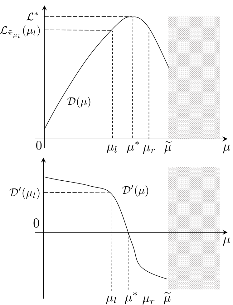
We illustrate this issue in the example in Fig. 2. We display a qualitative plot of the Lagrangian dual $\mathcal{D}(\mu)$ and its derivative $\mathcal{D}^{\prime}(\mu)$ when (21) admits a maximum at $\mu^{*}$ and the dichotomy search returned values $\mu_{l}$ and $\mu_{r}$ that are $\epsilon$ -close and $\mu^{*}\in[\mu_{l},\mu_{r}]$ . We consider the case where the algorithm returns $\mu_{l}$ as the candidate solution. By concavity and the fact that $\mathcal{D}^{\prime}(0)>0$ , the function $\mathcal{D}(\mu)$ is Lipschitz in the interval $[0,\mu^{*})$ with constant bounded by $\mathcal{D}^{\prime}(0)$ . Thus the accuracy $\mu^{*}-\mu_{l}\leq\epsilon$ translates into an equivalent $\epsilon$ -optimality in $\mathcal{D}$ (i.e., $\mathcal{D}(\mu^{*})-\mathcal{D}(\mu_{l})=\mathcal{L}^{*}-\mathcal{L}_{\widetilde{\pi}_{\mu_{l}}}(\mu_{l})\leq\mathcal{D}^{\prime}(0)\epsilon$ ). Nonetheless, this does not imply a similar guarantee for $D^{\prime}(\mu)$ . If the second derivative of $\mathcal{D}(\mu)$ (i.e., the curvature of the function) is large close to $\mu^{*}$ , the original error $\epsilon$ can be greatly amplified when evaluating $\mathcal{D}^{\prime}(\mu_{l})$ . For instance, if $\mathcal{D}^{\prime\prime}(\mu)\gg 1/\epsilon$ , then $\mathcal{D}^{\prime}(\mu_{l})=\Omega(1)$ . Given the last point of lemma 5, this means that despite returning an $\epsilon$ -optimal solution in the sense of (21), $\widetilde{\pi}_{\mu_{l}}$ may significantly violate the constraint (as $\mathcal{D}^{\prime}(\mu_{l})=g_{\widetilde{\pi}_{\mu_{l}}}=\Omega(1)$ ). While Eq. (25) implies that $\widetilde{\pi}_{\mu_{l}}$ is still optimistic (i.e., $\mathcal{J}_{\widetilde{\pi}_{\mu_{l}}}\leq J^{\star}$ , as in lemma 3), the regret accumulated by $\widetilde{\pi}_{\mu_{l}}$ cannot be controlled anymore, since the pertubration control $w_{s}$ may be arbitrarily outside the confidence interval. Interestingly, the curvature becomes larger and larger as the optimum shifts to the extremum of $\mathcal{M}$ and, in the limit, (21) only admits a supremum. In this case, no matter how close $\mu_{l}$ is to $\mu^{*}$ , the associated policy $\widetilde{\pi}_{\mu_{l}}$ may perform arbitrarily bad.

More formally, we have the following lemma (the explicit value of $\alpha$ is reported in Lem. 14).

Lemma 6.

For any LQR parametrized by $\widehat{\theta}$ , $V$ , $\beta$ , and psd cost matrices $Q,R$ , consider the domain $\mathcal{M}=[0,\widetilde{\mu})$ where Thm. 2 holds. Let $\mathcal{M}_{+}$ be a subset of $\mathcal{M}$ such that $\mathcal{M}_{+}=\{\mu\in\mathcal{M}\text{ s.t. }\mathcal{D}^{\prime}(\mu)\geq 0\}.$ Then, $\mathcal{D}$ has Lipschitz gradient, i.e., there exists a constant $\alpha$ depending on $\widehat{\theta}$ , $V$ , $\beta$ , and the cost matrices $Q,R$ , such that for all $(\mu_{1},\mu_{2})\in\mathcal{M}_{+}^{2}$ ,

|\mathcal{D}^{\prime}(\mu_{1})-\mathcal{D}^{\prime}(\mu_{2})|\leq|\mu_{1}-\mu_{2}|\frac{\alpha}{\lambda_{\min}(D_{\mu_{1}})},

where $D_{\mu}$ is defined in (24).

This result shows that even when $|\mu_{1}\!-\!\mu_{2}|\leq\epsilon$ , the difference in gradients may be arbitrarily large when $\lambda_{\min}(D_{\mu})\ll\epsilon$ (i.e., large curvature). In the next section, we build on this lemma to craft an adaptive stopping condition for the dichotomy search and to detect that case of large curvature.

5.2 An Efficient Dichotomy Search

Refer to caption — Figure 1: Qualitative plots of $\mathcal{D}(\mu)$ and its derivative $\mathcal{D}^{\prime}(\mu)$ .

The algorithm we propose, DS-OFU, seeks to find a value of $\mu$ of zero gradient $\mathcal{D}^{\prime}(\mu)$ by dichotomy search. While $\mathcal{D}(\mu)$ is a 1-dim function and Lem. 5 guarantees that it is concave in $\mathcal{M}$ , there are three major challenges to address: 1) Thm. 2 does not provide any explicit value for $\widetilde{\mu}$ ; 2) The algorithm needs to evaluate $\mathcal{D}^{\prime}(\mu)$ ; 3) For any $\epsilon$ , DS-OFU must return a policy $\widetilde{\pi}_{\epsilon}$ that is $\epsilon$ -optimistic and $\epsilon$ -feasible for the extended LQR with relaxed constraints (4.1).

DS-OFU starts by checking the sign of the gradient $\mathcal{D}^{\prime}(0)$ . If $\mathcal{D}^{\prime}(0)\leq 0$ , the algorithm ends and outputs the optimal policy $\widetilde{\pi}_{0}$ since by concavity $0$ is the arg-max of $\mathcal{D}$ and $\widetilde{\pi}_{0}$ is the exact solution to (21). If $\mathcal{D}^{\prime}(0)>0$ , the dichotomy starts with accuracy $\epsilon$ and a valid⁸⁸ 8 We say that $[\mu_{l},\mu_{r}]$ is valid if $\mathcal{D}^{\prime}(\mu_{l})\geq 0$ and $\mathcal{D}^{\prime}(\mu_{r})\leq 0$ . search interval $[0,\mu_{\max}]$ , where $\mu_{\max}$ is defined as follows.

Lemma 7.

Let $\mu_{\max}:=\beta^{-2}\lambda_{\max}\big(C\big)\lambda_{\max}(V)$ , then $\mathcal{D}^{\prime}(\mu_{\max})<0$ .

The previous lemma does not imply that $[0,\mu_{\max}]\supseteq\mathcal{M}$ , but it provides an explicit value of $\mu$ with negative gradient, thus defining a bounded and valid search interval for the dichotomy process. At each iteration, DS-OFU updates either $\mu_{l}$ or $\mu_{r}$ so that the interval $[\mu_{l},\mu_{r}]$ is always valid.

The second challenge is addressed in the following proposition, which illustrates how the derivative $\mathcal{D}^{\prime}(\mu)$ (equivalently the constraint $g_{\widetilde{\pi}_{\mu}}$ ) can be efficiently computed.

Proposition 3.

For any $\mu\in\mathcal{M}$ , let $\widetilde{\pi}_{\mu}$ (Eq. 23) have an associated controller $\widetilde{K}_{\mu}$ that induces a closed-loop dynamics $A^{\mathsf{c}}(\widetilde{K}_{\mu})=\widehat{A}+\widetilde{B}\widetilde{K}_{\mu}$ then $\mathcal{D}^{\prime}(\mu)=g_{\widetilde{\pi}_{\mu}}=\text{Tr}\big(G_{\mu}\big)$ , where $G_{\mu}$ is the unique solutions of the Lyapunov equation

G_{\mu}=\big(A^{\mathsf{c}}(\widetilde{K}_{\mu})\big)^{\mathsf{T}}G_{\mu}A^{\mathsf{c}}(\widetilde{K}_{\mu})+\begin{pmatrix}I\\ \widetilde{K}_{\mu}\end{pmatrix}^{\mathsf{T}}C_{g}\begin{pmatrix}I\\ \widetilde{K}_{\mu}\end{pmatrix},

This directly from the fact that $g_{\widetilde{\pi}}$ is an asymptotic average quadratic quantity (as much as the average cost $J$ ), and it is thus the solution of a Lyapunov equation of dimension $n$ .

The remaining key challenge is to design an adaptive stopping condition that is able to keep refining the interval $[\mu_{l},\mu_{r}]$ until either an accurate enough solution is returned, or, the curvature is too large (or even infinite). In the latter case, the algorithm switches to a failure mode, for which we design an ad-hoc solution.

Since the objective is to achieve an $\epsilon$ -feasible solution (i.e., $g_{\widetilde{\pi}_{\overline{\mu}}}\leq\epsilon$ ), we leverage lemma 6 and we interrupt the dichotomy process whenever $(\mu_{r}-\mu_{l})\alpha/\lambda_{\min}(D_{\mu_{l}})\leq\epsilon$ . Nonetheless, when the optimum of (21) is not attainable in $\mathcal{M}$ , the previous stopping condition may never be verified and the algorithm would never stop. As a result, we interrupt the dichotomy process when $\lambda_{\min}(D_{\mu_{l}})\leq\lambda_{0}\epsilon^{2}$ for a given constant $\lambda_{0}$ . In this case, the dichotomy fails to return a viable solution and we need to revert to a backup strategy, which consists in either modifying the controller found at $\mu_{l}$ or applying a suitable perturbation to the original cost matrix $C_{\dagger}$ . In the latter case, we design a perturbation such that 1) the optimization problem (21) associated to the system with the perturbed cost $C_{\dagger}^{\prime}$ admits a maximum and can be efficiently solved by the same dichotomy process illustrated before and 2) the corresponding solution $\widetilde{\pi}^{\prime}$ is $\epsilon$ -optimistic and $\epsilon$ -feasible in the original system. The explicit backup strategy is reported in App. I.

Theorem 3.

For any LQR parametrized by $\widehat{\theta}$ , $V$ , $\beta$ , and psd cost matrices $Q,R$ , and any accuracy $\epsilon\in(0,1/2)$ , there exists values of $\alpha$ and $\lambda_{0}$ and a backup strategy such that

1.

DS-OFU outputs an $\epsilon$ -optimistic and $\epsilon$ -feasible policy $\widetilde{\pi}_{\epsilon}$ given by the linear controller $\widetilde{K}_{\epsilon}$ such that

$\mathcal{J}_{\widetilde{\pi}_{\epsilon}}\leq\mathcal{J}_{*}+\epsilon\quad\text{ and }\quad g_{\widetilde{\pi}_{\epsilon}}\leq\epsilon.$
2.

DS-OFU terminates within at most $N=O\big(\log(\mu_{\max}/\epsilon)\big)$ iterations, each solving one Riccati and one Lyapunov equation for the extended Lagrangian LQR, both with complexity $O\big(n^{3}\big)$ .

This result shows that DS-OFU returns a solution to (4.1) at any level of accuracy $\epsilon$ in a total runtime $O(n^{3}\log(1/\epsilon))$ . We refer to the algorithm resulting by plugging DS-OFU into the OFU-LQ++ learning scheme as LagLQ (Lagrangian-LQ). By running DS-OFU with $\epsilon=1/\sqrt{t}$ provides the regret guarantee of theorem 1.

6 Discussion

We investigate the difference between confidence-based and isotropic exploration in term of complexity, bounds and empirical performance. While not conclusive, we believe this discussion sheds light on how confidence-based methods may be better at adapting to the structure of the problem. As a representative for isotropic exploration, we refer to CECCE (Simchowitz & Foster 2020), which offers the tightest regret guarantee among the CE strategies. For confidence-based exploration, we discuss the guarantee of both OFU-LQ++ and LagLQ, but limit the computational and experiment comparisons with LagLQ only.

Computational complexity. Both LagLQ and CECCE proceeds through episodes of increasing length. LagLQ relies on the standard determinant-based rule ( $\det(V_{t})\geq 2\det(V_{t_{k}})$ ) to decide when to stop, while in CECCE the length of each episode is twice longer than the previous one. In both cases, the length of the episodes is increasing exponentially over time, thus leading to $O(\log T)$ updates. Given the complexity analysis in theorem 3, we notice that DS-OFU and computing the CE controller have the same order of complexity, where CECCE solves one Riccati equation, while DS-OFU solves as many as $\log(1/\epsilon)$ Riccati and Lyapunov equations. On systems of moderate side and given the small number of recomputations, the difference between the two approaches is relatively narrow.

Regret. We limit the comparison to the main order term $\widetilde{O}(\sqrt{T})$ and the dependencies on dimensions $n$ and $d$ , and problem-dependent constants such as $\kappa$ and $\|P^{*}\|_{2}$ ,

	$\displaystyle\mathcal{R}_{{\small\textsc{CECCE}}}$	$\displaystyle=\widetilde{O}\big(\\|P^{*}\\|_{2}^{11/2}d\sqrt{nT}\big),$
	$\displaystyle\mathcal{R}_{{\small\textsc{OFU-LQ++}}}$	$\displaystyle=\widetilde{O}\big(\kappa^{1/2}\\|P_{*}\\|^{3/2}_{2}(n+d)\!\sqrt{n}\sqrt{T}\big),$
	$\displaystyle\mathcal{R}_{{\small\textsc{LagLQ}}}$	$\displaystyle=\widetilde{O}\big(\kappa^{3/2}\\|P_{*}\\|_{2}^{2}(n+d)\sqrt{n}\sqrt{T}\big).$

The first difference is that CECCE has worst-case optimal dependency $d\sqrt{n}$ on the dimension of the problem, while optimistic algorithms OFU-LQ++ and LagLQ are slightly worse, scaling with $(n+d)\sqrt{n}$ . While this shows that OFU-LQ++ and LagLQ are worst-case optimal when $n\approx d$ , it is an open question whether $\epsilon-$ greedy is by nature superior to confidence-based method when $d\ll n$ or whether it is due to a loose analysis. In fact, those dependencies are mostly inherited from the confidence intervals in (1) which is treated differently in (Simchowitz & Foster 2020), thanks to a refined bound and a different regret decomposition. This suggests that a finer analysis for OFU-LQ++ and LagLQ may close this gap.

The main difference lies in the dependency on complexity-related quantities $\kappa$ and $\|P^{*}\|_{2}$ . While there is no strict ordering between them,⁹⁹ 9 The definition of $\kappa=D/\lambda_{\min}{Q}$ , with $D\geq\text{Tr}(P^{*})$ may suggest $\kappa>\|P^{*}\|_{2}$ , but the smallest eigenvalue of $Q$ may be large enough so that $\kappa\leq\|P^{*}\|_{2}$ . they both measure the cost of controlling the system. In this respect, CECCE suffers from a significantly larger dependency than optimistic algorithms: OFU-LQ++ offers the best performance while LagLQ is slightly worse than OFU-LQ++, due to the use of a relaxed constraint to obtain tractability. We believe this difference in performance may be intrinsic in the fact that methods based on isotropic perturbations of the CE are less effective in adapting to the actual structure of the problem. As the isotropic perturbation is tuned to guarantee a sufficient estimation in all directions of the state-control space, it leads to over-exploration w.r.t. some directions as soon as there is an asymmetry in the cost sensitivity in the estimation error. On the other hand, OFU-LQ++ and LagLQ further leverage this asymmetry from the confidence set, and by optimism, do not waste exploration to learn accurately directions which have little to no impact on the performance.

Empirical comparison. We conclude with a simple numerical simulation (details in App. J). We compare CECCE with the variance parameter ( $\sigma_{in}^{2}$ ) set as suggested in the original paper and a tuned version where we shrink it by a factor $\sqrt{\|P_{*}\|_{2}}$ , and LagLQ where the confidence interval is set according to (1). Both algorithms receive the same set $\Theta_{0}$ obtained from an initial system identification phase. In Fig. 3 we see that LagLQ performs better than both the original and tuned versions of CECCE. More interestingly, while CECCE is “constrained” to have a $O(\sqrt{T})$ regret by the definition of the perturbation itself, which scales as $1/\sqrt{t}$ , it seems LagLQ’s regret is $o(\sqrt{T})$ , suggesting that despite the worst-case lower bound $\Omega(\sqrt{T})$ , LagLQ may be adapt to the structure of the problem and achieve better regret.

References

Abbasi-Yadkori & Szepesvári (2011) Abbasi-Yadkori, Y. and Szepesvári, C. Regret bounds for the adaptive control of linear quadratic systems. In COLT, pp. 1–26, 2011.
Abbasi-Yadkori et al. (2011) Abbasi-Yadkori, Y., Pál, D., and Szepesvári, C. Online least squares estimation with self-normalized processes: An application to bandit problems. arXiv preprint arXiv:1102.2670, 2011.
Abeille & Lazaric (2018) Abeille, M. and Lazaric, A. Improved regret bounds for thompson sampling in linear quadratic control problems. In Proceedings of the 35th International Conference on Machine Learning, ICML 2018, Stockholmsmässan, Stockholm, Sweden, July 10-15, 2018, pp. 1–9, 2018.
Bittanti et al. (2006) Bittanti, S., Campi, M., et al. Adaptive control of linear time invariant systems: the “bet on the best” principle. Communications in Information & Systems, 6(4):299–320, 2006.
Cohen et al. (2019) Cohen, A., Koren, T., and Mansour, Y. Learning linear-quadratic regulators efficiently with only $\sqrt{T}$ regret. CoRR, abs/1902.06223, 2019. URL http://arxiv.org/abs/1902.06223.
Dean et al. (2018) Dean, S., Mania, H., Matni, N., Recht, B., and Tu, S. Regret bounds for robust adaptive control of the linear quadratic regulator. CoRR, abs/1805.09388, 2018. URL http://arxiv.org/abs/1805.09388.
Faradonbeh et al. (2017) Faradonbeh, M. K. S., Tewari, A., and Michailidis, G. Finite time analysis of optimal adaptive policies for linear-quadratic systems. CoRR, abs/1711.07230, 2017. URL http://arxiv.org/abs/1711.07230.
Faradonbeh et al. (2018a) Faradonbeh, M. K. S., Tewari, A., and Michailidis, G. Finite time adaptive stabilization of LQ systems. CoRR, abs/1807.09120, 2018a. URL http://arxiv.org/abs/1807.09120.
Faradonbeh et al. (2018b) Faradonbeh, M. K. S., Tewari, A., and Michailidis, G. Input perturbations for adaptive regulation and learning. CoRR, abs/1811.04258, 2018b. URL http://arxiv.org/abs/1811.04258.
Jaksch et al. (2010) Jaksch, T., Ortner, R., and Auer, P. Near-optimal regret bounds for reinforcement learning. J. Mach. Learn. Res., 11:1563–1600, August 2010.
Lancaster & Rodman (1995) Lancaster, P. and Rodman, L. Algebraic riccati equations. Oxford University Press, 1995.
Mania et al. (2019) Mania, H., Tu, S., and Recht, B. Certainty Equivalent Control of LQR is Efficient. arXiv e-prints, art. arXiv:1902.07826, Feb 2019.
Molinari (1975) Molinari, B. P. The stabilizing solution of the discrete algebraic riccati equation. Automatic Control, IEEE Transactions on, 20(3):396–399, Jun 1975.
Ouyang et al. (2017) Ouyang, Y., Gagrani, M., and Jain, R. Learning-based control of unknown linear systems with thompson sampling. CoRR, abs/1709.04047, 2017. URL http://arxiv.org/abs/1709.04047.
Rockafellar (1970) Rockafellar, R. T. Convex analysis. Number 28. Princeton university press, 1970.
Rugh (1996) Rugh, W. J. Linear system theory, volume 2. prentice hall Upper Saddle River, NJ, 1996.
Simchowitz & Foster (2020) Simchowitz, M. and Foster, D. J. Naive Exploration is Optimal for Online LQR. arXiv e-prints, art. arXiv:2001.09576, Jan 2020.
Van Dooren (1981) Van Dooren, P. A generalized eigenvalue approach for solving riccati equations. SIAM Journal on Scientific and Statistical Computing, 2(2):121–135, 1981.

Appendix A Notation

We recall the basic notation defined in the paper and introduce additional convenient notation.

Linear algebra.

•

$\lambda(A)$ : the spectrum of the matrix $A$
•

$\rho(A)$ : the spectral radius of a matrix $A$ , $\rho(A)=\max|\lambda(A)|$
•

$\lambda_{\min}(M)$ , $\lambda_{\max}(M)$ : the minimum and maximum eigenvalue of a symmetric matrix $M$
•

$Im(A)$ , $\ker(A)$ : the row and null space of a matrix $A$
•

$|x|$ : the absolute value (resp. the modulus) of $x\in\mathbb{R}$ (resp. $x\in\mathbb{C}$ )
•

$\|x\|$ : the euclidian norm of a vector $x$
•

$\|A\|_{2}$ : the $2-$ norm of a matrix $A$ , $\|A\|_{2}=\max_{\|x\|=1}\|Ax\|$
•

$\|A\|_{F}$ : the Frobenius norm of a matrix $A$ , $\|A\|_{F}=\sqrt{\text{Tr}(A^{\mathsf{T}}A)}$
•

$\|A\|_{M}$ : the weighted Frobenius norm of $A$ wrt to a psd matrix $M$ , $\|A\|_{M}=\|M^{1/2}A\|_{F}$

Original LQR problem.

•

$n,d$ : the dimensions of the state and input variables
•

$x_{t},u_{t},\epsilon_{t}$ : the state/input/noise variables at time $t$
•

$z_{t}$ : aggregated state and input variable at time $t$ , $z_{t}^{\mathsf{T}}=(x_{t}^{\mathsf{T}},u_{t}^{\mathsf{T}})$
•

$A_{*},B_{*}$ : ground truth for the state dynamics parameters
•

$Q,R$ : cost matrices of the LQR
•

$C$ : aggregated cost matrix, $C=(Q,0;0,R)$
•

$\pi$ , $K$ : an arbitrary linear policy mapping states to inputs, and its matrix representation.
•

$\theta$ : aggregated state dynamics parametrization, $\theta^{\mathsf{T}}=(A,B)$
•

$P(\theta)$ : solution of the Riccati equation associated with the LQR system parametrized by $\theta$ and $C$
•

$K(\theta)$ : optimal controller for the LQR system parametrized by $\theta$ and $C$
•

$A^{\mathsf{c}}(\theta,K)$ : the closed-loop matrix of a dynamical system parametrized by $\theta$ controlled by $K$ , $A^{\mathsf{c}}(\theta,K)=\theta^{\mathsf{T}}\begin{pmatrix}I\\ K\end{pmatrix}$
•

$A^{\mathsf{c}}(\theta)$ : the closed-loop matrix of a dynamical system parametrized by $\theta$ controlled by $K(\theta)$ , $A^{\mathsf{c}}(\theta)=A^{\mathsf{c}}(\theta,K(\theta))$
•

$\Sigma(\theta,K)$ : The steady-state covariance of the state process driven by $A^{\mathsf{c}}(\theta,K)$
•

$J_{\pi}(\theta)$ : the infinite horizon cost of an LQR parametrized by $\theta$ and controlled by $\pi$
•

$J(\theta)$ : the infinite horizon cost of an LQR parametrized by $\theta$ and optimally controlled by $K(\theta)$
•

$J_{*}$ : the optimal infinite horizon cost for the true LQR system, $J_{*}=J(\theta_{*})$

Extended/Lagrangian LQR problem.

•

$w_{t}$ : the input perturbation at time $t$
•

$\widetilde{u}_{t}$ : the extended input at time $t$ , $\widetilde{u}_{t}^{\mathsf{T}}=(u_{t}^{\mathsf{T}},w_{t}^{\mathsf{T}})$
•

$C_{\dagger}$ , $C_{g}$ : the cost matrices of the extended LQR objective and constraint
•

$\widetilde{B}$ : the extended input matrix, $\widetilde{B}=(B,I)$
•

$\widetilde{\pi}$ , $\widetilde{K}$ : an arbitrary linear extended policy mapping states to extended inputs, and its matrix representation
•

$\mathcal{J}_{\widetilde{\pi}}(\theta,\beta,V)$ : the infinite horizon cost of the constrained extended LQR parametrized by $(\theta,\beta,V)$ and controlled by $\widetilde{\pi}$
•

$\mathcal{J}_{*}$ : the optimal infinite horizon cost of the constrained extended LQR.
•

$g_{\widetilde{\pi}}(\theta,\beta,V)$ : the infinite horizon constraint value of the constrained extended LQR parametrized by $(\theta,\beta,V)$ and controlled by $\widetilde{\pi}$
•

$\mathcal{L}_{\widetilde{\pi}}(\theta,\beta,V;\cdot)$ : the Lagrangian function associated with the extended constrained LQR
•

$\mathcal{D}(\cdot)$ : the dual function associated with the Lagrangian relaxation

Appendix B Structure of the Appendix

The appendix is organized over different sections:

•

appendix C recalls elements of Lyapunov stability theory and concentration inequality (high-probability events) (proposition 1).
•

appendix D contains the proofs of OFU-LQ++ (sequential stability lemma 1 and regret lemma 2).
•

appendix E contains the proofs of LagLQ (optimism lemma 3, sequential stability lemma 4, and regret theorem 1) .
•

Appendices F,G, H reports the strong-duality proofs (theorem 2, lemma 5, lemma 6, lemma 7, proposition 3).
•

appendix I details the algorithms and the proof of theorem 3.
•

appendix J details the experimental protocol used to obtain Fig. 3.

At the beginning of each part we recall and complement the notation used in that specific part.

Appendix C Preliminaries

C.1 Lyapunov Stability

We recall basic results from Lyapunov stability theory. Most of the definitions below are adapted from Rugh 1996. We consider a general discrete-time deterministic linear dynamical process $\{\overline{x}_{t}\}_{t\geq 0}$ with dynamics $A$ and initial state $\xi$ defined as

\displaystyle\overline{x}_{t+1}=A\overline{x}_{t},\quad\overline{x}_{0}=\xi.

(26)

We recall the following definition of stability.

Definition 1.

A deterministic process (26) is uniformly exponentially stable (UES) if there exists a constant $\gamma>0$ and a constant $0\leq\lambda<1$ such that for any $t\geq s\geq 0$ ,

\displaystyle\|\overline{x}_{t}\|\leq\gamma\lambda^{t-s}\|\overline{x}_{s}\|.

(27)

The stability of the deterministic process (26) can be translated into stability properties of the transition matrix $A$ . The following propositions provide spectral characterizations.

Proposition 4 (Thm. 22.1 (Rugh 1996)).

A time-invariant deterministic process (26) is uniformly exponentially stable if and only if all eigenvalues of $A$ have magnitude strictly smaller than 1, i.e., $\rho(A)<1$ .

Proposition 5 (Thm. 22.7 (Rugh 1996)).

The process (26) is uniformly exponentially stable (UES) if and only if there exists a constant $\gamma>0$ and a constant $0\leq\lambda<1$ such that for all $t\geq s$ , $\|A^{t-s}\|\leq\gamma\lambda^{t-s}$ .

An alternative characterization is provided by Lyapunov stability theory.

Proposition 6 (Thm. 23.3 (Rugh 1996)).

A deterministic process (26) is uniformly exponentially stable if and only if there exists a symmetric p.s.d. matrix $\Sigma$ such that

\Sigma=A\Sigma A^{\mathsf{T}}+I.

(28)

Further, let $\rho$ be finite positive constants such that $\Sigma\preccurlyeq\rho I$ , then for any $t\geq s\geq 0$ , we have $\|A^{t-s}\|\leq\gamma\lambda^{t-s}$ with

\gamma=\sqrt{\rho},\quad\lambda=1-1/\rho.

(29)

Uniform exponential stability for a deterministic process directly implies boundedness for a perturbed version of the process with bounded perturbations.

Proposition 7.

Consider the perturbed instance $\{\widetilde{x}_{t}\}_{t\geq 0}$ of the deterministic process (26), defined as

\widetilde{x}_{t+1}=A\widetilde{x}_{t}+\epsilon_{t},\quad\widetilde{x}_{0}=\xi,\quad\text{ for all }t\geq 0.

(30)

where $\{\epsilon_{t}\}_{t\geq 0}$ is a martingale difference sequence with zero-mean, $\sigma-$ subGaussian increments. If the deterministic process is UES associated with a psd matrix $\Sigma$ given in eq. 28, the perturbed process $\{\widetilde{x}_{t}\}_{t\geq 0}$ is uniformly bounded, that is, with probability at least $1-\delta$ ,

\text{for all }t\geq 0,\quad\|\widetilde{x}_{t}-A^{t}\xi\|^{2}\leq 8\sigma^{2}\text{Tr}(\Sigma)\log(1/\delta).

(31)

Proof of Prop. 7.

First we use eq. 30 to reformulate the perturbed process as

\widetilde{x}_{t}=A^{t}\xi+\sum_{s=1}^{t}A^{t-s}\epsilon_{s-1}.

(32)

Then, we follow similar steps as in Abbasi-Yadkori et al. 2011: we begin by constructing an exponential super-martingale. Formally, for all $\alpha\in\mathbb{R}^{n}$ ,

M_{t}^{\alpha}=\exp\left(\alpha^{\mathsf{T}}(\widetilde{x}_{t}-A^{t}\xi)-\frac{\sigma^{2}}{2}\|\alpha\|^{2}_{\sum_{s=1}^{t}A^{t-s}(A^{t-s})^{\mathsf{T}}}\right),

is a super-martingale, and $\mathbb{E}(M^{\alpha}_{t})\leq 1$ . By eq. 32, we have for any $s\geq 0$ ,

\mathbb{E}(M^{\alpha}_{s}|\mathcal{F}_{s-1})=M_{s-1}^{\alpha}\mathbb{E}\left(\alpha^{\mathsf{T}}A^{t-s}\epsilon_{s-1}-\frac{\sigma^{2}}{2}\alpha^{\mathsf{T}}A^{t-s}\big(A^{t-s}\big)^{\mathsf{T}}\alpha\Big|\mathcal{F}_{s-1}\right)\leq M_{s-1}^{\alpha},

which ensures that $M^{\alpha}_{t}$ is a super-martingale while $M^{\alpha}_{0}=1$ ensures that $\mathbb{E}(M^{\alpha}_{t})\leq 1$ . Further, recursively applying eq. 28 ensures that:

\text{for all }t\geq 0,\quad\sum_{s=1}^{t}A^{t-s}\big(A^{t-s}\big)^{\mathsf{T}}\preccurlyeq\Sigma.

Following Abbasi-Yadkori et al. 2011, we consider the random variable $\mathcal{A}\sim\mathcal{N}(0,\sigma^{-2}\lambda_{\max}(\Sigma)^{-1}I)$ , independent of the noise sequence $\{\epsilon_{s}\}_{s\geq 0}$ and obtain, by the tower rule, that for all $t\geq 0$ , $M_{t}=\mathbb{E}_{\mathcal{A}}(M^{\mathcal{A}}_{t})$ is such that $\mathbb{E}(M_{t})\leq 1$ . Further,

	$\displaystyle M_{t}$	$\displaystyle\geq\sqrt{\frac{\det\left(\sigma^{2}\lambda_{\max}(\Sigma)I\right)}{(2\pi)^{n}}}\int_{\alpha\in\mathbb{R}^{n}}\exp\left(\alpha^{\mathsf{T}}(\widetilde{x}_{t}-A^{t}\xi)-\frac{\sigma^{2}}{2}\\|\alpha\\|^{2}_{\Sigma+\lambda_{\max}(\Sigma)I}\right)$
		$\displaystyle=\exp\left(\frac{1}{2\sigma^{2}}\\|\widetilde{x}_{t}-A^{t}\xi\\|^{2}_{(\Sigma+\lambda_{\max}(\Sigma)I)^{-1}}\right)\sqrt{\frac{\det\left(\sigma^{2}\lambda_{\max}(\Sigma)I\right)}{\det\left(\sigma^{2}(\Sigma+\lambda_{\max}(\Sigma)I)\right)}}$
		$\displaystyle=\exp\left(\frac{1}{2\sigma^{2}}\\|\widetilde{x}_{t}-A^{t}\xi\\|^{2}_{(\Sigma+\lambda_{\max}(\Sigma)I)^{-1}}\right)\sqrt{\frac{\det\left(\lambda_{\max}(\Sigma)I\right)}{\det\left(\Sigma+\lambda_{\max}(\Sigma)I\right)}}$

We conclude as in Cor. 1 in (Abbasi-Yadkori et al. 2011) using Markov inequality and a stopping time construction to obtain that with probability at least $1-\delta$ ,

\text{for all }t\geq 0,\;\;\;\;\|\widetilde{x}_{t}-A^{t}\xi\|^{2}\leq 2\sigma^{2}\lambda_{\max}(\Sigma)\log\left(\frac{\det\left(\Sigma+\lambda_{\max}(\Sigma)I\right)}{\det\left(\lambda_{\max}(\Sigma)I\right)}\right)+4\sigma^{2}\lambda_{\max}(\Sigma)\log(1/\delta).

Finally, from $\log(1+x)\leq x$ , we obtain

\lambda_{\max}(\Sigma)\log\left(\frac{\det\left(\Sigma+\lambda_{\max}(\Sigma)I\right)}{\det\left(\lambda_{\max}(\Sigma)I\right)}\right)\leq\text{Tr}(\Sigma),\quad\lambda_{\max}(\Sigma)\leq\text{Tr}(\Sigma),

which leads to, with probability at least $1-\delta$ ,

\text{for all }t\geq 0,\;\;\;\;\|\widetilde{x}_{t}-A^{t}\xi\|^{2}\leq 8\sigma^{2}\text{Tr}(\Sigma)\log(1/\delta).

∎

C.2 Technical results on Lyapunov stability

We recall useful technical results on Lyapunov manipulations.

Proposition 8 (Thm. 23.7 (Rugh 1996)).

Given a $n\times n$ matrix $A$ , if there exists symmetric positive definite $n\times n$ matrices $M$ and $P$ satisfying the discrete time Lyapunov equation

A^{\mathsf{T}}PA-P=-M

(33)

then all eigenvalues of $A$ have magnitude strictly smaller than 1 (i.e., $\rho(A)<1$ ) and $A$ is stable. Conversely, if $\rho(A)<1$ , then for every p.s.d. matrix $M$ , the solution of Eq. 33 exists and is unique.

While the above theorem is stated for some matrix $A$ , in the following we rely extensively on a similar characterization but for $A^{\mathsf{T}}$ . As $A^{\mathsf{T}}$ and $A$ have the same spectrum, Prop. 8 can be rephrased in term of $A^{\mathsf{T}}$ .

Corollary 1.

Given a $n\times n$ matrix $A$ , if there exists a symmetric, positive definite $n\times n$ matrices $M$ and $\Sigma$ satisfying the discrete time Lyapunov equation

A\Sigma A^{\mathsf{T}}-\Sigma=-M

(34)

then all eigenvalues of $A$ have magnitude strictly less than one (i.e., $\rho(A)<1$ ) and $A$ is stable. Conversely, if $\rho(A)<1$ , then for every p.s.d. matrix $M$ , the solution of Eq. 33 exists and is unique.

Proposition 9.

Let $A$ be stable and $(\Sigma_{1},M_{1})$ , and $(\Sigma_{2},M_{2})$ be pairs of p.s.d. matrices satisfying the Lyapunov equations

A\Sigma_{1}A^{\mathsf{T}}-\Sigma_{1}=-M_{1};\quad\quad A\Sigma_{2}A^{\mathsf{T}}-\Sigma_{2}=-M_{2}.

If $M_{1}\preccurlyeq M_{2}$ , then $\Sigma_{1}\preccurlyeq\Sigma_{2}$ .

Proposition 10.

Let $A$ be stable and $(\Sigma_{1},M)$ , and $(\Sigma_{2},\alpha M)$ be pairs of p.s.d. matrices satisfying the Lyapunov equations

A\Sigma_{1}A^{\mathsf{T}}-\Sigma_{1}=-M;\quad\quad A\Sigma_{2}A^{\mathsf{T}}-\Sigma_{2}=-\alpha M.

Then, $\Sigma_{2}=\alpha\Sigma_{1}$ .

Proposition 11.

Let $A$ be stable and $M$ be a psd matrix. Let $P$ and $\Sigma$ be solution the Lyapunov equations

A^{\mathsf{T}}PA-P=-M;\quad\quad A\Sigma A^{\mathsf{T}}-\Sigma=-I.

Then, $\text{Tr}(P)=\text{Tr}(\Sigma M)$ .

We finally provide a technical result that we will intensively use in sections D.1 and E.2. This proposition shows that the stability property of some matrix $A_{0}$ will be preserved for all matrix $A_{1}$ sufficiently close to $A_{0}$ , where the distance between $A_{0}$ and $A_{1}$ is measured according to a Lyapunov metric associated with $A_{0}$ .

Proposition 12.

Let $A_{0}\in\mathbb{R}^{n\times n}$ be a stable matrix, and let $\Sigma_{0}$ be the steady-state covariance associated with $A_{0}$ satisfying the Lyapunov:

\Sigma_{0}=A_{0}\Sigma_{0}A_{0}^{\mathsf{T}}+I.

For any matrix $A_{1}$ such that $\|(A_{0}-A_{1})^{\mathsf{T}}\|_{\Sigma_{0}}\leq\eta c_{0}$ where $c_{0}^{2}\eta(\eta+2)<1$ and $c_{0}\geq\|A_{0}^{\mathsf{T}}\|_{\Sigma_{0}}$ , then,

1.

$A_{1}$ is stable, and we denote by $\Sigma_{1}$ its steady-state covariance matrix defined as the unique solution of

$\Sigma_{1}=A_{1}\Sigma_{1}A_{1}^{\mathsf{T}}+I,$
2.

$\Sigma_{1}\preccurlyeq\frac{1}{1-c_{0}^{2}\eta(\eta+2)}\Sigma_{0}$ .

Proof.

We first prove that $A_{1}$ is stable by corollary 1. Algebraic manipulations lead to

	$\displaystyle A_{1}\Sigma_{0}A_{1}^{\mathsf{T}}$	$\displaystyle=A_{0}\Sigma_{0}A_{0}^{\mathsf{T}}+(A_{1}-A_{0})\Sigma_{0}(A_{1}-A_{0})^{\mathsf{T}}+A_{0}\Sigma_{0}(A_{1}-A_{0})^{\mathsf{T}}+(A_{1}-A_{0})\Sigma_{0}A_{0}^{\mathsf{T}}$
		$\displaystyle=\Sigma_{0}-I+M,$

where $M=(A_{1}-A_{0})\Sigma_{0}(A_{1}-A_{0})^{\mathsf{T}}+A_{0}\Sigma_{0}(A_{1}-A_{0})^{\mathsf{T}}+(A_{1}-A_{0})\Sigma_{0}A_{0}^{\mathsf{T}}$ . As a result, corollary 1 guarantees the stability of $A_{1}$ whenever $\|M\|_{2}<1$ . Further, this is asserted since

	$\displaystyle\\|M\\|_{2}$	$\displaystyle\leq\\|\Sigma_{0}^{1/2}(A_{1}-A_{0})^{\mathsf{T}}\\|^{2}_{2}+2\\|\Sigma_{0}^{1/2}(A_{1}-A_{0})^{\mathsf{T}}\\|_{2}\\|\Sigma_{0}^{1/2}A_{0}^{\mathsf{T}}\\|_{2}\leq\\|(A_{1}-A_{0})^{\mathsf{T}}\\|^{2}_{\Sigma_{0}}+2\\|(A_{1}-A_{0})^{\mathsf{T}}\\|_{\Sigma_{0}}\\|A_{0}^{\mathsf{T}}\\|_{\Sigma_{0}}$
		$\displaystyle\leq c_{0}^{2}\big(\eta^{2}+2\eta\big)<1.$

We now characterize the distance in term of stability between $A_{0}$ and $A_{1}$ , showing how $\Sigma_{1}$ relates to $\Sigma_{0}$ (in a psd sense). Let $\Delta=\Sigma_{1}-\Sigma_{0}$ . Then, algebraic manipulations leads to

	$\displaystyle\Delta$	$\displaystyle=A_{1}\Delta A_{1}^{\mathsf{T}}+(A_{1}-A_{0})\Sigma_{0}(A_{1}-A_{0})^{\mathsf{T}}+(A_{1}-A_{0})\Sigma_{0}A_{0}^{\mathsf{T}}+A_{0}\Sigma_{0}(A_{1}-A_{0})^{\mathsf{T}}$
		$\displaystyle=A_{1}\Delta A_{1}^{\mathsf{T}}+M.$

From $M\preccurlyeq\|M\|_{2}I$ , we obtain that $\Delta\preccurlyeq Z$ where $Z=A_{1}ZA_{1}^{\mathsf{T}}+\|M\|_{2}I$ by proposition 9 which can be expressed as $Z=\|M\|_{2}\Sigma_{1}$ by proposition 10. As a result, we have

\Delta\preccurlyeq\|M\|_{2}\Sigma_{1}\quad\quad\Rightarrow\quad\quad\Sigma_{1}\preccurlyeq\frac{1}{1-\|M\|_{2}}\Sigma_{0},

which concludes the proof since $\|M\|_{2}\leq c_{0}^{2}\big(\eta^{2}+2\eta\big)$ .

∎

C.3 High-probability events

All the derivations provided in appendices D and E will be conducted under the high-probability events that $\theta_{*}$ belongs to the confidence ellipsoid associated with the RLS procedure. Formally, we consider the event

E_{t}=\Big\{\forall\hskip 2.84526pts\leq t,\hskip 2.84526pt\theta_{*}\in C_{s}\Big\},

where $\mathcal{C}_{t}$ is defined in eq. 9. By proposition 1 and from $\beta_{t}=\beta_{t}(\delta/4)$ , $E_{T}$ holds with probability at least $1-\delta/4$ . This result is standard and we report the proofs here for sake of completeness.

Proof of proposition 1.

The proof of proposition 1 is essentially the same as the one of Abbasi-Yadkori & Szepesvári 2011 but for the way the RLS is regularized. We provide it for sake of completeness.
Using the expression of $\widehat{\theta}_{t}$ , one gets:

\displaystyle\widehat{\theta}_{t}

\displaystyle=V_{t}^{-1}\left(\theta_{0}+\sum_{s=0}^{t-1}z_{s}x_{s+1}^{\mathsf{T}}\right)=V_{t}^{-1}\left(\lambda\theta_{0}+\sum_{s=0}^{t-1}z_{s}z_{s}^{\mathsf{T}}\theta_{*}+\sum_{s=0}^{t-1}z_{s}\epsilon_{s+1}^{\mathsf{T}}\right)=V_{t}^{-1}\left(\lambda\theta_{0}+(V_{t}-\lambda I)\theta_{*}+\sum_{s=0}^{t-1}z_{s}\epsilon_{s+1}^{\mathsf{T}}\right)

which leads to

\|\widehat{\theta}_{t}-\theta_{*}\|_{V_{t}}\leq\lambda\|\theta_{0}-\theta_{*}\|_{V_{t}^{-1}}+\|S_{t}\|_{V_{t}^{-1}},

where $S_{t}=\sum_{s=0}^{t-1}z_{s}\epsilon_{s+1}^{\mathsf{T}}$ . We decompose $S_{t}=(S_{t}^{1},\dots,S_{t}^{n})$ as

S_{t}^{i}=\sum_{s=0}^{t-1}z_{s}\epsilon_{s+1}^{i},\hskip 8.53581pt\forall i\in\{1,\dots,n\}

where $\{\epsilon_{s}^{i}\}_{s\geq 0}$ is a martingale difference sequence, with zero-mean $\sigma$ -subGaussian increment. From Cor. 1 in (Abbasi-Yadkori et al. 2011), for any $0<\delta<1$ , we have with probability at least $1-\delta$ :

\forall t\geq 0,\hskip 8.53581pt\|S_{t}^{i}\|_{V_{t}^{-1}}\leq\sigma\sqrt{2\log\Big(\frac{\det(V_{t})^{1/2}}{\det(\lambda I)^{1/2}\delta}\Big)}.

Finally, a union bound argument leads to:

\forall t\geq 0,\hskip 8.53581pt\|S_{t}\|_{V_{t}^{-1}}\leq\sigma\sqrt{2n\log\Big(\frac{\det(V_{t})^{1/2}n}{\det(\lambda I)^{1/2}\delta}\Big)}.

which concludes the proof. ∎

Appendix D Sequential Stability and Regret of OFU-LQ++

This section is dedicated to the proofs of lemma 1 and lemma 2. We first address the sequential stability of OFU-LQ++ (section D.1) and then show how it translates in a regret bound that scales polynomially with the dimension and the problem dependent constant $\kappa$ ( section D.2). All the results in the section are derived under 1, 2 and 3.

Notations. We recall the LQR notation used in this section. We consider LQR systems of the form eq. 1, whose dynamics is characterized by matrices $A\in\mathbb{R}^{n\times n}$ and $B\in\mathbb{R}^{n\times d}$ and cost matrix characterized by $C=\begin{pmatrix}Q&0\\ 0&R\end{pmatrix}$ . We summarize these parameters as $\theta^{\mathsf{T}}=(A\;\;B)\in\mathbb{R}^{n\times(n+d)}$ .
Given an arbitrary control matrix $K\in\mathbb{R}^{d\times n}$ , we denote by $A^{\mathsf{c}}(\theta,K)=A+BK\in\mathbb{R}^{n\times n}$ the associated closed-loop matrix. We often use $L^{\mathsf{T}}=\big(I\;\;K^{\mathsf{T}}\big)\in\mathbb{R}^{n\times(n+d)}$ , so that the closed-loop matrix can be written as $A^{\mathsf{c}}(\theta,K)=\theta^{\mathsf{T}}L$ .

Whenever $A^{c}(\theta,K)$ is stable, we denote as $P(\theta,K)$ the (unique) p.s.d. matrix satisfying the Lyapunov equation (see (33))

P(\theta,K)=A^{\mathsf{c}}(\theta,K)^{\mathsf{T}}P(\theta,K)A^{c}(\theta,K)+Q+K^{\mathsf{T}}RK.

(35)

Notice that $\text{Tr}(P(\theta,K))$ represents the average cost of the LQ problem parametrized with $\theta$ under control $K$ . In a similar fashion, we denote as $\Sigma(\theta,K)$ the steady-state covariance satisfying (see (34))

\Sigma(\theta,K)=A^{\mathsf{c}}(\theta,K)\Sigma(\theta,K)A^{\mathsf{c}}(\theta,K)^{\mathsf{T}}+I.

(36)

Furthermore, whenever $\theta$ is stabilizable, we denote by $K(\theta)$ the associated optimal control and $L(\theta)^{\mathsf{T}}=\big(I\;K(\theta)^{\mathsf{T}}\big)$ . When $\theta$ is controlled by $K(\theta)$ we often use the shorthand notation $A^{\mathsf{c}}(\theta)=A^{\mathsf{c}}(\theta,K(\theta))$ , $\Sigma(\theta)=\Sigma(\theta,K(\theta))$ and $P(\theta)=P(\theta,K(\theta))$ .
The parameters of the true system are summarized in $\theta_{*}^{\mathsf{T}}=(A_{*}\;\;B_{*})\in\mathbb{R}^{n\times(n+d)}$ and we denote as $K_{*}$ , $L_{*}$ , $P_{*}$ and $\Sigma_{*}$ the optimal quantities $K(\theta_{*})$ , $L(\theta_{*})$ , $P(\theta_{*},K_{*})$ and $\Sigma(\theta_{*},K_{*})$ respectively.

OFU-LQ++. At each time step $t\geq 0$ , OFU-LQ++ maintains an estimates $\widehat{\theta}_{t}$ of $\theta_{*}$ together with a confidence set $\mathcal{C}_{t}$ as given eqs. 5 and 9. OFU-LQ++ proceeds in episodes, triggered when $\det(V_{t})\geq 2\det(V_{t_{k}})$ , and at the beginning of each episode $k$ , OFU-LQ++ selects an optimistic parameters $\theta_{t_{k}}\in\mathcal{C}_{t_{k}}$ and computes the optimal controller $K(\theta_{t_{k}})$ associated with $\theta_{t_{k}}$ . Then, the optimistic controller $K(\theta_{t_{k}})$ is used until the end of the episode.
The optimistic nature of $\theta_{t_{k}}$ and $K(\theta_{t_{k}})$ ensures that for all $k\geq 0$ , $\text{Tr}\big(P(\theta_{t_{k}},K(\theta_{t_{k}}))\big)\leq\text{Tr}(P_{*})\leq D$ on the high-probability event $\theta_{*}\in\mathcal{C}_{t_{k}}$ .

D.1 Sequential stability of OFU-LQ++

The proof of the sequential stability of OFU-LQ++ is derived on the high-probability event $E_{T}$ and is conducted in two steps.
Step 1) We show that OFU-LQ++ outputs a sequence of stable controller $\{K(\theta_{t_{k}})\}_{k\geq 1}$ (i.e., such that $A^{\mathsf{c}}(\theta_{*},K(\theta_{t_{k}}))$ is UES) as long as $\|\theta_{t_{k}}-\theta_{*}\|\leq 2\epsilon_{0}$ for $\epsilon_{0}$ satisfying

\kappa\eta(\epsilon_{0})\leq 1;\quad\quad\eta(\epsilon_{0}):=4\kappa\epsilon_{0}(1+\epsilon_{0})<1,

where $\kappa=D/\lambda_{\min}(C)$ .
Step 2) We prove lemma 1 showing that $\|\theta_{t_{k}}-\theta_{*}\|\leq 2\epsilon_{0}$ does hold for a suitable initialization phase and choice of regularization parameter $\lambda$ , by induction. This allows us to construct recursively a high-probability event over which the state process remains bounded.

D.1.1 Step 1

The following proposition summarizes how optimism translates into stability properties.

Proposition 13.

Assume that $\theta_{*}\in\mathcal{C}_{t}$ for all $t\geq 0$ . Let $\{\theta_{t_{k}}\}_{k\geq 1}$ and $\{K(\theta_{t_{k}})\}_{k\geq 1}$ be the sequence of optimistic parameters/controllers generated by OFU-LQ++ over episodes $k\geq 0$ . Then, under 2 and 3, for all $k\geq 0$ ,

1.

$\theta_{t_{k}}$ is a stabilizable system and $A^{\mathsf{c}}(\theta_{t_{k}},K(\theta_{t_{k}}))$ is stable,

$\|L(\theta_{t_{k}})^{\mathsf{T}}\|_{\Sigma(\theta_{t_{k}},K(\theta_{t_{k}}))}\leq\sqrt{\kappa}$ and $\|\Sigma(\theta_{t_{k}},K(\theta_{t_{k}}))^{1/2}\|_{F}\leq\sqrt{\kappa}$ , where $\kappa=D/\lambda_{\min}(C)$ and

\Sigma(\theta_{t_{k}},K(\theta_{t_{k}}))=A^{\mathsf{c}}(\theta_{t_{k}},K(\theta_{t_{k}}))\Sigma(\theta_{t_{k}},K(\theta_{t_{k}}))A^{\mathsf{c}}(\theta_{t_{k}},K(\theta_{t_{k}}))^{\mathsf{T}}+I.

3.

$\|L(\theta_{t_{k}})\|_{F}\leq\sqrt{\kappa}$ and $\|A^{\mathsf{c}}(\theta_{t_{k}},K(\theta_{t_{k}}))^{\mathsf{T}}\|_{\Sigma(\theta_{t_{k}},K(\theta_{t_{k}}))}\leq\sqrt{\kappa}$ .

Proof.

1.

By construction of $\theta_{t_{k}}$ and $K(\theta_{t_{k}})$ , optimism guarantees stability of the closed-loop matrix $A^{\mathsf{c}}(\theta_{t_{k}},K(\theta_{t_{k}}))$ . Indeed, if $A^{\mathsf{c}}(\theta_{t_{k}},K(\theta_{t_{k}}))$ was unstable, we would have $\text{Tr}(P(\theta_{t_{k}}),K(\theta_{t_{k}})))=+\infty$ , which contradicts the optimistic property $\text{Tr}(P(\theta_{t_{k}}K(\theta_{t_{k}})))\leq\text{Tr}(P_{*})\leq D<+\infty$ . As a result, $A^{\mathsf{c}}(\theta_{t_{k}},K(\theta_{t_{k}}))$ is stable and $\theta_{t_{k}}$ is a stabilizable pair.

By definition, we have

	$\displaystyle P(\theta_{t_{k}},K(\theta_{t_{k}})$	$\displaystyle=A^{\mathsf{c}}(\theta_{t_{k}},K(\theta_{t_{k}}))^{\mathsf{T}}P(\theta_{t_{k}},K(\theta_{t_{k}}))A^{\mathsf{c}}(\theta_{t_{k}},K(\theta_{t_{k}}))+L(\theta_{t_{k}})^{\mathsf{T}}CL(\theta_{t_{k}}),$
	$\displaystyle\Sigma(\theta_{t_{k}},K(\theta_{t_{k}}))$	$\displaystyle=A^{\mathsf{c}}(\theta_{t_{k}},K(\theta_{t_{k}}))\Sigma(\theta_{t_{k}},K(\theta_{t_{k}}))A^{\mathsf{c}}(\theta_{t_{k}},K(\theta_{t_{k}}))^{\mathsf{T}}+I.$

Then, applying proposition 11 with $M=L(\theta_{t_{k}})^{\mathsf{T}}CL(\theta_{t_{k}})$ leads to

D\geq\text{Tr}\big(P(\theta_{t_{k}},K(\theta_{t_{k}}))\big)=\text{Tr}\big(\Sigma(\theta_{t_{k}},K(\theta_{t_{k}}))M).

Noticing that $M\succcurlyeq\lambda_{\min}(C)L(\theta_{t_{k}})^{\mathsf{T}}L(\theta_{t_{k}})$ we obtain that

D\geq\text{Tr}\big(P(\theta_{t_{k}},K(\theta_{t_{k}}))\big)\geq\text{Tr}\big(\Sigma(\theta_{t_{k}},K(\theta_{t_{k}}))L(\theta_{t_{k}})^{\mathsf{T}}L(\theta_{t_{k}})\big)\lambda_{\min}(C)=\lambda_{\min}(C)\|L(\theta_{t_{k}})^{\mathsf{T}}\|^{2}_{\Sigma(\theta_{t_{k}},K(\theta_{t_{k}}))}.

Similarly, from $M\succcurlyeq Q+K(\theta_{t_{k}})^{\mathsf{T}}RK(\theta_{t_{k}})\succcurlyeq Q\succcurlyeq\lambda_{\min}(C)I$ we obtain

D\geq\text{Tr}\big(P(\theta_{t_{k}},K(\theta_{t_{k}}))\big)\geq\text{Tr}\big(\Sigma(\theta_{t_{k}},K(\theta_{t_{k}}))\big)\lambda_{\min}(C)=\lambda_{\min}(C)\|\Sigma(\theta_{t_{k}},K(\theta_{t_{k}}))^{1/2}\|_{F}^{2}.

We conclude using that $\kappa=D/\lambda_{\min}(C)$ .

3.

The last assertions come directly from the previous one, noticing that $\Sigma(\theta_{t_{k}},K(\theta_{t_{k}}))\succcurlyeq I$ and $A^{\mathsf{c}}(\theta_{t_{k}},K(\theta_{t_{k}}))\Sigma(\theta_{t_{k}},K(\theta_{t_{k}}))A^{\mathsf{c}}(\theta_{t_{k}},K(\theta_{t_{k}}))^{\mathsf{T}}\preccurlyeq\Sigma(\theta_{t_{k}},K(\theta_{t_{k}}))$ .

∎

Equipped with those properties, we now show that for any $k\geq 0$ , the optimistic controller $K(\theta_{t_{k}})$ stabilizes the true system parameterized by $\theta_{*}$ , as long as $\theta_{t_{k}}$ is sufficiently close to $\theta_{*}$ and characterize the stability margin in term of steady-state covariance and cost.

Proposition 14.

Let $k\geq 0$ and assume that $\theta_{*}\in\mathcal{C}_{t_{k}}$ . Let $\theta_{t_{k}}$ and $K(\theta_{t_{k}})$ be an optimistic parameter/control pair. Then, if $\|\theta_{t_{k}}-\theta_{*}\|_{F}\leq 2\epsilon_{0}$ where $\epsilon_{0}$ is such that $\eta(\epsilon_{0}):=4\kappa\epsilon_{0}(1+\epsilon_{0})<1$ , under 2 and 3,

1.

$A^{\mathsf{c}}(\theta_{*},K(\theta_{t_{k}}))$ is stable,
2.

$\Sigma(\theta_{*},K(\theta_{t_{k}}))\preccurlyeq\frac{1}{1-\eta(\epsilon_{0})}\Sigma(\theta_{t_{k}},K(\theta_{t_{k}}))$ ,
3.

$\big\|P\big(\theta_{*},K(\theta_{t_{k}})\big)\big\|_{2}\preccurlyeq\big\|P\big(\theta_{*},K(\theta_{*}))\big\|_{2}+\frac{D\eta(\epsilon_{0})}{1-\eta(\epsilon_{0})}$ ,
4.

$\big\|P\big(\theta_{t_{k}},K(\theta_{t_{k}})\big)\|_{2}\leq\big\|P\big(\theta_{*},K(\theta_{*}))\big\|_{2}(1+\kappa\eta(\epsilon_{0})/2)+\frac{D\eta(\epsilon_{0})}{1-\eta(\epsilon_{0})}(1+\kappa\eta(\epsilon_{0})/2)$ .

Proof.

The first two assertions directly follows from propositions 13 and 12. From

\left\|\left(A^{\mathsf{c}}(\theta_{*},K(\theta_{t_{k}}))-A^{\mathsf{c}}(\theta_{t_{k}},K(\theta_{t_{k}}))\right)^{\mathsf{T}}\right\|_{\Sigma(\theta_{t_{k}},K(\theta_{t_{k}}))}\leq\|\theta_{*}-\theta_{t_{k}}\|_{F}\|L(\theta_{t_{k}})^{\mathsf{T}}\|_{\Sigma(\theta_{t_{k}},K(\theta_{t_{k}}))}\leq 2\epsilon_{0}\sqrt{\kappa}

and

\left\|A^{\mathsf{c}}(\theta_{t_{k}},K(\theta_{t_{k}}))^{\mathsf{T}}\right\|_{\Sigma(\theta_{t_{k}},K(\theta_{t_{k}}))}\leq\sqrt{\kappa},

we can apply proposition 12 with $A_{0}=A^{\mathsf{c}}(\theta_{t_{k}},K(\theta_{t_{k}}))$ , $A_{1}=A^{\mathsf{c}}(\theta_{*},K(\theta_{t_{k}}))$ , $\eta=2\epsilon_{0}$ and $c_{0}=\sqrt{\kappa}$ , which leads to the desired result.

Let $\Delta=P\big(\theta_{*},K(\theta_{t_{k}})\big)-P\big(\theta_{*},K(\theta_{*})\big)$ and $\eta(\epsilon_{0})=4\kappa\epsilon_{0}(1+\epsilon_{0})$ . We have

	$\displaystyle\\|\Delta\\|_{2}=\lambda_{\max}(\Delta)$	$\displaystyle\leq\text{Tr}\Big(P\big(\theta_{},K(\theta_{t_{k}})\big)\Big)-\text{Tr}\Big(P\big(\theta_{},K(\theta_{*})\big)\Big)$
		$\displaystyle=\text{Tr}\Big(P\big(\theta_{},K(\theta_{t_{k}})\big)\Big)-\text{Tr}\Big(P\big(\theta_{t_{k}},K(\theta_{t_{k}})\big)\Big)+\text{Tr}\Big(P\big(\theta_{t_{k}},K(\theta_{t_{k}})\big)\Big)-\text{Tr}\Big(P\big(\theta_{},K(\theta_{*})\big)\Big)$
		$\displaystyle\leq\text{Tr}\Big(P\big(\theta_{*},K(\theta_{t_{k}})\big)\Big)-\text{Tr}\Big(P\big(\theta_{t_{k}},K(\theta_{t_{k}})\big)\Big),$

where we used that by optimism, $\text{Tr}\big(P(\theta_{t_{k}},K(\theta_{t_{k}}))\big)-\text{Tr}\big(P(\theta_{*},K(\theta_{*}))\big)\leq 0$ . Using that

	$\displaystyle\text{Tr}\left(P\big(\theta_{*},K(\theta_{t_{k}})\big)\right)$	$\displaystyle=\text{Tr}\left(L(\theta_{t_{k}})^{\mathsf{T}}CL(\theta_{t_{k}})\Sigma(\theta_{*},K(\theta_{t_{k}}))\right)$
	$\displaystyle\text{Tr}\left(P\big(\theta_{t_{k}},K(\theta_{t_{k}})\big)\right)$	$\displaystyle=\text{Tr}\left(L(\theta_{t_{k}})^{\mathsf{T}}CL(\theta_{t_{k}})\Sigma(\theta_{t_{k}},K(\theta_{t_{k}}))\right)$

we obtain

\lambda_{\max}(\Delta)\leq\text{Tr}\left(L(\theta_{t_{k}})^{\mathsf{T}}CL(\theta_{t_{k}})\big(\Sigma(\theta_{*},K(\theta_{t_{k}}))-\Sigma(\theta_{t_{k}},K(\theta_{t_{k}}))\big)\right).

Finally, from $\Sigma(\theta_{*},K(\theta_{t_{k}}))-\Sigma(\theta_{t_{k}},K(\theta_{t_{k}}))\preccurlyeq\frac{\eta(\epsilon_{0})}{1-\eta(\epsilon_{0})}\Sigma(\theta_{t_{k}},K(\theta_{t_{k}}))$ we have

\lambda_{\max}(\Delta)\leq\frac{\eta(\epsilon_{0})}{1-\eta(\epsilon_{0})}\text{Tr}\left(L(\theta_{t_{k}})^{\mathsf{T}}CL(\theta_{t_{k}})\Sigma(\theta_{t_{k}},K(\theta_{t_{k}}))\right)=\frac{\eta(\epsilon_{0})}{1-\eta(\epsilon_{0})}\text{Tr}\big(P(\theta_{t_{k}},K(\theta_{t_{k}}))\big)\leq\frac{D\eta(\epsilon_{0})}{1-\eta(\epsilon_{0})}.

Let $\Delta=P\big(\theta_{t_{k}},K(\theta_{t_{k}})\big)-P\big(\theta_{*},K(\theta_{t_{k}})\big)$ and $\eta(\epsilon_{0})=4\kappa\epsilon_{0}(1+\epsilon_{0})$ . We have

	$\displaystyle\Delta$	$\displaystyle=A^{\mathsf{c}}(\theta_{t_{k}},K_{t_{k}})^{\mathsf{T}}\Delta A^{\mathsf{c}}(\theta_{t_{k}},K_{t_{k}})+A^{\mathsf{c}}(\theta_{t_{k}},K_{t_{k}})^{\mathsf{T}}P\big(\theta_{},K(\theta_{t_{k}})\big)A^{\mathsf{c}}(\theta_{t_{k}},K_{t_{k}})-A^{\mathsf{c}}(\theta_{},K_{t_{k}})^{\mathsf{T}}P\big(\theta_{},K(\theta_{t_{k}})\big)A^{\mathsf{c}}(\theta_{},K_{t_{k}})$
		$\displaystyle\leq A^{\mathsf{c}}(\theta_{t_{k}},K_{t_{k}})^{\mathsf{T}}\Delta A^{\mathsf{c}}(\theta_{t_{k}},K_{t_{k}})+\epsilon_{0}^{2}\\|L_{t}\\|_{2}^{2}\\|P\big(\theta_{},K(\theta_{t_{k}})\big)\\|_{2}+2\epsilon_{0}\\|L_{t}\\|_{2}\\|P\big(\theta_{},K(\theta_{t_{k}})\big)\\|_{2}$
		$\displaystyle\leq A^{\mathsf{c}}(\theta_{t_{k}},K_{t_{k}})^{\mathsf{T}}\Delta A^{\mathsf{c}}(\theta_{t_{k}},K_{t_{k}})+(\epsilon_{0}^{2}\kappa+2\epsilon_{0}\sqrt{\kappa})\\|P\big(\theta_{*},K(\theta_{t_{k}})\big)\\|_{2},$
		$\displaystyle\leq A^{\mathsf{c}}(\theta_{t_{k}},K_{t_{k}})^{\mathsf{T}}\Delta A^{\mathsf{c}}(\theta_{t_{k}},K_{t_{k}})+\frac{1}{2}\eta(\epsilon_{0})\\|P\big(\theta_{*},K(\theta_{t_{k}})\big)\\|_{2}.$

which implies that $\|\Delta\|_{2}\leq\kappa\eta(\epsilon_{0})/2\|P\big(\theta_{*},K(\theta_{t_{k}})\big)\|_{2}$ . Combined with the previous point, we obtain,

\big\|P\big(\theta_{t_{k}},K(\theta_{t_{k}})\big)\big\|_{2}\leq\big\|P\big(\theta_{*},K(\theta_{t_{k}})\big)\big\|_{2}(1+\kappa\eta(\epsilon_{0})/2)\leq\big\|P\big(\theta_{*},K(\theta_{*})\big\|_{2}(1+\kappa\eta(\epsilon_{0})/2)+\frac{D\eta(\epsilon_{0})}{1-\eta(\epsilon_{0})}(1+\kappa\eta(\epsilon_{0})/2)

∎

We conclude Step 1) showing that whenever $\theta_{t_{k}}$ is sufficiently close to $\theta_{*}$ for all $t\geq 1$ , the sequence of optimistic controller $\{K(\theta_{t_{k}})\}_{k\geq 1}$ induces a state process $\{x_{t}\}_{t\geq 1}$ for each episode $k$ given by

x_{t+1}=A^{\mathsf{c}}(\theta_{*},K(\theta_{t_{k}}))x_{t}+\epsilon_{t},\quad\quad\forall t\in[t_{k},t_{k+1}-1],

(37)

that is uniformly exponentially stable.

Proposition 15.

Assume that $\theta_{*}\in\mathcal{C}_{t}$ for all $t\geq 0$ . Let $\{\theta_{t_{k}}\}_{k\geq 1}$ and $\{K(\theta_{t_{k}})\}_{k\geq 1}$ be the sequence of optimistic parameters/controls pair. Then, if for all $k\geq 0$ , $\|\theta_{t_{k}}-\theta_{*}\|\leq 2\epsilon_{0}$ where $\epsilon_{0}$ is such that

\kappa\eta(\epsilon_{0})\leq 1;\quad\quad\eta(\epsilon_{0}):=4\kappa\epsilon_{0}(1+\epsilon_{0})\leq 1/2,

(38)

under 1, 2 and 3,

1.

for all $k$ , the state process in eq. 37 is uniformly exponentially stable,

for all $k$ , for any $0<\delta<1$ , with probability at least $1-\delta$ ,

\text{for all }t\in[t_{k},t_{k+1}-1],\quad\begin{aligned} \|x_{t}\|&\leq 4\sigma\sqrt{\kappa\log(1/\delta)}+\sqrt{\kappa}(1-1/\kappa)^{t}\|x_{t_{k}}\|\\ \|x_{t}\|&\leq 4\sigma\sqrt{\kappa\log(1/\delta)}+2\sqrt{\big\|P(\theta_{*},K(\theta_{*}))\big\|_{2}/\lambda_{\min}(C)}\|x_{t_{k}}\|.\end{aligned}

(39)

Proof.

By propositions 13 and 14, it exists $\Sigma_{k}=\Sigma(\theta_{*},K(\theta_{t_{k}}))$ such that

\Sigma_{k}=A^{\mathsf{c}}(\theta_{*},K(\theta_{t_{k}}))\Sigma_{k}A^{\mathsf{c}}(\theta_{*},K(\theta_{t_{k}}))^{\mathsf{T}}+I,\quad\quad\text{Tr}(\Sigma_{k})\leq\kappa.

As a result, proposition 6 ensures that the process in eq. 37 is uniformly exponentially stable.

Noticing that $t_{k+1}=\inf\{t\geq t_{k}\text{ s.t. }\det(V_{t})>2\det(V_{t_{k}})\}$ is a stopping time, we obtain the first bound in the second assertion directly by applying propositions 6 and 7. To obtain the second bound, we use proposition 14

	$\displaystyle\\|A^{\mathsf{c}}(\theta_{*},K(\theta_{t_{k}}))^{t}\xi\\|$	$\displaystyle\leq\\|A^{\mathsf{c}}(\theta_{},K(\theta_{t_{k}}))^{t}\\|_{2}\\|\xi\\|\leq\big\\|\sqrt{P(\theta_{},K(\theta_{t_{k}}))\big\\|_{2}/\lambda_{\min}(C)}\\|\xi\\|$
		$\displaystyle\leq\sqrt{\big\\|P(\theta_{},K(\theta_{}))\big\\|_{2}/\lambda_{\min}(C)+1}\\|\xi\\|$
		$\displaystyle\leq 2\sqrt{\big\\|P(\theta_{},K(\theta_{}))\big\\|_{2}/\lambda_{\min}(C)}\\|\xi\\|.$

∎

D.1.2 Step 2. Proof of lemma 1

Let $X:=20\sigma\sqrt{\kappa\log(4T/\delta)}\sqrt{\big\|P(\theta_{*},K(\theta_{*}))\big\|_{2}/\lambda_{\min}(C)}$ , we are now ready to construct recursively a sequence of high-probability events

F_{t}=\Big\{\forall\hskip 2.84526pts\leq t,\hskip 2.84526pt\|x_{s}\|\leq X\Big\}

over which the state process remains bounded. We work on $\{E_{t}\}_{t\leq T}$ and we proceed by episode on the increasing sequence of probability events $\{E_{t_{k}}\cap F_{t_{k}}\}_{k\geq 1}$ .

Proof of lemma 1.

We assume that OFU-LQ++ is initialized with a stabilizing set $\Theta_{0}=\{\theta:\|\theta-\theta_{0}\|\leq\epsilon_{0}\}$ such that $\epsilon_{0}$ satisfies

\kappa\eta(\epsilon_{0}^{\prime})\leq 1;\quad\quad\eta(\epsilon_{0}^{\prime}):=4\kappa\epsilon_{0}^{\prime}(1+\epsilon_{0}^{\prime})\leq 1/2;\quad\quad\epsilon_{0}^{\prime}=2\epsilon_{0}.

Further, we assume that the RLS estimation in eq. 6 is instantiated with

\lambda=\frac{2n\sigma^{2}}{\epsilon_{0}^{2}}\Big(\log(4n/\delta)+(n+d)\log\Big(1+\kappa X^{2}T\Big)\Big).

Setting $\epsilon_{0}\leq\frac{1}{32\kappa^{2}}$ ensures that $\eta(\epsilon_{0}^{\prime})\leq 1/2$ , $\kappa\eta(\epsilon_{0}^{\prime})\leq 1$ and that $\lambda\geq 4^{3}\sigma^{2}\kappa^{4}\log(4T/\delta)/\log(2)$ .

We now proceed by induction, for sake of simplicity, we assume that $x_{0}=0$ . We show that w.h.p.

1)

$\|x_{t}\|\leq X:=20\sigma\sqrt{\kappa\log(4T/\delta)}\sqrt{\big\|P(\theta_{*},K(\theta_{*}))\big\|_{2}/\lambda_{\min}(C)}$ for all $t\in[t_{k},t_{k+1}]$
2)

$\|x_{t_{k+1}}\|\leq 8\sigma\sqrt{\kappa\log(4T/\delta)}$ .

•

At $k=0$ , $\theta_{t_{0}}\in\mathcal{C}_{0}$ implies that

\|\theta_{t_{0}}-\theta_{*}\|\leq 2\beta_{t_{0}}\big/\sqrt{\lambda_{\min}(V_{t_{0}})}=2\big(\epsilon_{0}+\sigma\sqrt{2n\log(4n/\delta)}/\sqrt{\lambda}\big)\leq 4\epsilon_{0}:=2\epsilon_{0}^{\prime}.

As a result, proposition 15 guarantees that with probability at least $1-\delta/4T$ ,

\text{for all }s\leq t_{1},\quad\|x_{s}\|\leq 4\sigma\sqrt{\kappa\log(4T/\delta)}+2\sqrt{\big\|P(\theta_{*},K(\theta_{*}))\big\|_{2}/\lambda_{\min}(C)}\|x_{0}\|\leq X\quad\text{ and }\quad\|x_{t_{1}}\|\leq 8\sigma\sqrt{\kappa\log(4T/\delta)}.

Hence, $\mathbb{P}(F_{t_{1}}|E_{t_{0}})\geq 1-\delta/4T$ .

•

At $k+1$ , assume that $E_{t_{k}}\cap F_{t_{k}}$ holds. From $\|x_{s}\|\leq X$ for all $s\leq t_{k+1}$ , we obtain that

	$\displaystyle\beta_{t_{k+1}}$	$\displaystyle=\sigma\sqrt{2n\log\Big(\frac{\det(V_{t_{k+1}})^{1/2}4n}{\det(\lambda I)^{1/2}\delta}\Big)}+\lambda^{1/2}\\|\theta_{0}-\theta_{*}\\|_{F}$
		$\displaystyle\leq\sigma\sqrt{2n\log(4n/\delta)+2n(n+d)\log\Big(1+\sup_{s\leq t_{k+1}-1}\\|z_{s}\\|^{2}T\Big)}+\lambda^{1/2}\epsilon_{0}$
		$\displaystyle\leq\sigma\sqrt{2n\log(4n/\delta)+2n(n+d)\log\Big(1+\kappa X^{2}T\Big)}+\lambda^{1/2}\epsilon_{0}$
		$\displaystyle\leq 2\epsilon_{0}\sqrt{\lambda},$

where we used that $z_{s}=L(\theta_{s})x_{s}$ and $\|L(\theta_{s})\|_{2}\leq\sqrt{\kappa}$ by proposition 13, and the definition of $\lambda$ . As a result, $\|\theta_{t_{k+1}}-\theta_{*}\|\leq 2\epsilon_{0}^{\prime}$ and we can apply proposition 15. Using that $\|x_{t_{k}}\|\leq 8\sigma\sqrt{\kappa\log(4T/\delta)}$ we obtain with probability at least $1-\delta/4T$ ,

	$\displaystyle\text{for all }t_{k}\leq s\leq t_{k+1},\quad\\|x_{s}\\|$	$\displaystyle\leq 4\sigma\sqrt{\kappa\log(4T/\delta)}+2\sqrt{\big\\|P(\theta_{},K(\theta_{}))\big\\|_{2}/\lambda_{\min}(C)}\\|x_{t_{k}}\\|$
		$\displaystyle\leq 4\sigma\sqrt{\kappa\log(4T/\delta)}(1+4\sqrt{\big\\|P(\theta_{},K(\theta_{}))\big\\|_{2}/\lambda_{\min}(C)}$
		$\displaystyle\leq X.$

Hence, $\mathbb{P}(F_{t_{k+1}}|E_{t_{k}},F_{t_{k}})\geq 1-\delta/4T$ . Further, on this event,

\|x_{t_{k+1}}\|\leq 4\sigma\sqrt{\kappa\log(4T/\delta)}(1+\sqrt{\kappa}(1-1/\kappa)^{t_{k+1}-t_{k}+1})\leq 8\sigma\sqrt{\kappa\log(4T/\delta)}

which concludes the induction. To obtain the last inequality, we used that $t_{k+1}-t_{k}+1\geq\kappa\log(\kappa)/2$ since otherwise it enters in contradiction with the update rule: suppose that $t_{k+1}-t_{k}+1\leq\kappa\log(\kappa)/2$ ,

	$\displaystyle\det(V_{t_{k+1}})$	$\displaystyle\leq\det(V_{t_{k}})\prod_{t=t_{k}}^{t_{k+1}-1}(1+\\|z_{t}\\|^{2}_{V^{-1}_{t}})\leq\det(V_{t_{k}})\prod_{t=t_{k}}^{t_{k+1}-1}\big(1+\\|x_{t}\\|^{2}\kappa/\lambda\big)$
		$\displaystyle\leq\det(V_{t_{k}})\exp\Big(\frac{\kappa}{\lambda}\sum_{t=t_{k}}^{t_{k+1}-1}\\|x_{t}\\|^{2}\Big)\leq\det(V_{t_{k}})\exp\Big(32\sigma^{2}\kappa^{2}\log(4T/\delta)\big((t_{k+1}-t_{k}+1)+\kappa^{2}\big)/\lambda\Big)$
		$\displaystyle\leq\det(V_{t_{k}})\exp\Big(4^{3}\sigma^{2}\kappa^{4}\log(4T/\delta)/\lambda\Big)\leq 2\det(V_{t_{k}}),$

where we used that $\lambda\geq 4^{3}\sigma^{2}\kappa^{4}\log(4T/\delta)/\log(2)$ .

Overall, we showed that the sequence of event $F_{t}$ is such that $\mathbb{P}(F_{t_{k+1}}|F_{t_{k}},E_{t_{k}})\geq 1-\delta/4T$ for all $k\geq 0$ . As a result, we have

\mathbb{P}(F_{T}\cap E_{T})\geq\mathbb{P}(E_{T}\bigcap\cap_{k\geq 0}F_{t_{k}}|F_{t_{k-1}},E_{t_{k-1}})\geq 1-\mathbb{P}(E_{T}^{c})-\sum_{k\geq 0}\mathbb{P}\Big((F_{t_{k}}|F_{t_{k-1}},E_{t_{k-1}})^{c}\big)\geq 1-\delta/2.

∎

D.2 Regret bound for OFU-LQ++

The proof of lemma 2 follows from carefully using lemma 1 in the analysis of Abbasi-Yadkori & Szepesvári 2011. We provide it for sake of completeness. In line with Abbasi-Yadkori & Szepesvári 2011, we perform a regret decomposition on the sequence of events $\{E_{t}\cap F_{t}\}_{t\geq 0}$ and obtain

$\displaystyle R(T)=\sum_{t=0}^{T}x_{t}^{\mathsf{T}}Qx_{t}+u_{t}^{\mathsf{T}}Ru_{t}-J_{*}=$	$\displaystyle\sum_{t=0}^{T}J(\theta_{t})-J_{*}$	(40)
	$\displaystyle+\sum_{t=0}^{T}x_{t}^{\mathsf{T}}P_{t}x_{t}-\mathbb{E}\big(x_{t+1}^{\mathsf{T}}P_{t+1}x_{t+1}\|\mathcal{F}_{t}\big)$
	$\displaystyle+\sum_{t=0}^{T}\mathbb{E}\big(x_{t+1}^{\mathsf{T}}(P_{t+1}-P_{t})x_{t+1}\|\mathcal{F}_{t}\big)$
	$\displaystyle+\sum_{t=0}^{T}\big(\theta_{t}^{\mathsf{T}}z_{t}\big)^{\mathsf{T}}P_{t}\big(\theta_{t}^{\mathsf{T}}z_{t}\big)-\big(\theta_{}^{\mathsf{T}}z_{t}\big)^{\mathsf{T}}P_{t}\big(\theta_{}^{\mathsf{T}}z_{t}\big).$

where $\theta_{t}=\theta_{t_{k}}$ and $P_{t}=P(\theta_{t_{k}})$ for all $[t_{k},t_{k+1}-1]$ . $\theta_{t_{k}}$ is the optimistic parameter chosen by OFU-LQ++ at the beginning of episode $k$ . Each regret terms are then bounded separately as in Abbasi-Yadkori & Szepesvári 2011 but for the last term.

Bounding $R^{opt}(T)=\sum_{t=0}^{T}J(\theta_{t})-J_{*}$ .

Since $\theta_{t}$ is optimistic, on $E_{t}$ , $J(\theta_{t})\leq J_{*}$ . As a result, $R^{opt}(T)\leq 0$ . Further, by proposition 14 and the tuning of $\epsilon_{0}$ , $\|P_{t}\|_{2}=O\big(\|P(\theta_{*})\|_{2}\big)$ .

Bounding $R^{mart}(T)=\sum_{t=0}^{T}x_{t}^{\mathsf{T}}P_{t}x_{t}-\mathbb{E}\big(x_{t+1}^{\mathsf{T}}P_{t+1}x_{t+1}|\mathcal{F}_{t}\big)$ .

On $E_{t}\cap F_{t}$ , Lem. 1 guarantees that $\|x_{t}\|\leq X$ where $X=20\sigma\sqrt{\kappa\log(4T/\delta)}\sqrt{\big\|P(\theta_{*},K(\theta_{*}))\big\|_{2}/\lambda_{\min}(C)}$ . Thus, $R^{mart}(T)$ is a bounded martingale sequence and applying Azuma’s inequality leads to

R^{mart}(T)=\widetilde{O}\big(X^{2}\|P(\theta_{*})\|_{2}\sqrt{T}\big)=\widetilde{O}\big(\kappa\|P(\theta_{*})\|^{2}_{2}\sqrt{T}\big).

Bounding $R^{lazy}(T)=\sum_{t=0}^{T}\mathbb{E}\big(x_{t+1}^{\mathsf{T}}(P_{t+1}-P_{t})x_{t+1}|\mathcal{F}_{t}\big)$ .

The lazy update scheme used to re-evaluate the controllers $K_{t}$ s, ensures that the number of updates scales logarithmically. Hence, $R^{lazy}(T)=\widetilde{O}\big(X^{2}\|P(\theta_{*})\|_{2}(n+d)\big)$ .

Bounding $R^{pred}(T)=\sum_{t=0}^{T}\big(\theta_{t}^{\mathsf{T}}z_{t}\big)^{\mathsf{T}}P_{t}\big(\theta_{t}^{\mathsf{T}}z_{t}\big)-\big(\theta_{}^{\mathsf{T}}z_{t}\big)^{\mathsf{T}}P_{t}\big(\theta_{}^{\mathsf{T}}z_{t}\big)$ .

From the triangular inequality, we have:

	$\displaystyle R^{pred}(T)=\sum_{t=0}^{T}\\|\theta_{t}^{\mathsf{T}}z_{t}\\|^{2}_{P_{t}}-\\|\theta_{*}^{\mathsf{T}}z_{t}\\|_{P_{t}}^{2}$	$\displaystyle=\sum_{t=0}^{T}\big(\\|\theta_{t}^{\mathsf{T}}z_{t}\\|_{P_{t}}-\\|\theta_{}^{\mathsf{T}}z_{t}\\|_{P_{t}}\big)\big(\\|\theta_{t}^{\mathsf{T}}z_{t}\\|_{P_{t}}+\\|\theta_{}^{\mathsf{T}}z_{t}\\|_{P_{t}}\big)$
		$\displaystyle\leq\sum_{t=0}^{T}\\|(\theta_{t}-\theta_{})^{\mathsf{T}}z_{t}\\|_{P_{t}}\big(\\|\theta_{t}^{\mathsf{T}}z_{t}\\|_{P_{t}}+\\|\theta_{}^{\mathsf{T}}z_{t}\\|_{P_{t}}\big).$

Further, $\|\theta_{t}^{\mathsf{T}}z_{t}\|_{P_{t}}=\|A^{\mathsf{c}}(\theta_{t},K(\theta_{t})))x_{t}\|_{P_{t}}\leq\|x_{t}\|_{P_{t}}\leq\|P_{t}\|_{2}^{1/2}X$ . Similarly, on $E_{t}\cap F_{t}$ ,

	$\displaystyle\\|\theta_{*}^{\mathsf{T}}z_{t}\\|_{P_{t}}$	$\displaystyle\leq\\|\theta_{t}^{\mathsf{T}}z_{t}\\|_{P_{t}}+\\|A^{\mathsf{c}}(\theta_{*},K(\theta_{t}))x_{t}-A^{\mathsf{c}}(\theta_{t},K(\theta_{t}))x_{t}\\|_{P_{t}}$
		$\displaystyle\leq\\|P_{t}\\|_{2}^{1/2}X+4\\|P_{t}\\|_{2}^{1/2}X\sqrt{\kappa}\epsilon_{0}$
		$\displaystyle\leq 2X\\|P_{t}\\|_{2}^{1/2}.$

where we used $\|\theta_{t}-\theta_{*}\|\leq 2\epsilon_{0}$ from line 1 to 2, and the condition on $\epsilon_{0}$ from line 2 to 3. Thus,

R^{pred}(T)\leq 3X\|P_{t}\|_{2}\sum_{t=0}^{T}\|(\theta_{t}-\theta_{*})^{\mathsf{T}}z_{t}\|\leq 6X\|P_{t}\|_{2}\beta_{T}\sum_{t=1}^{T}\|z_{t}\|_{V_{t}^{-1}}.

Finally, noticing that $\kappa X^{2}/\lambda=O(1)$ , we have by eq. 7 that $\sum_{t=1}^{T}\|z_{t}\|_{V_{t}^{-1}}=\widetilde{O}\big(\sqrt{(n+d)T}\big)$ . Further, from $\|P_{t}\|_{2}=O\big(\|P(\theta_{*})\|_{2}\big)$ , $X=\widetilde{O}(\sqrt{\kappa\|P(\theta_{*})\|_{2}})$ and $\beta_{T}=\widetilde{O}(\sqrt{n(n+d)})$ , we obtain $R^{pred}(T)=\widetilde{O}\big(\sqrt{\kappa}\|P(\theta_{*})\|^{3/2}_{2}(n+d)\sqrt{n}\sqrt{T}\big)$ .

Appendix E Optimism, Sequential Stability and Regret of LagLQ

This section is dedicated to the proofs of LagLQ and concerns the Extended Optimistic LQR with Relaxed Constraints introduced in section 4. We first prove lemma 3 showing that LagLQ does use an optimistic controller (section E.1). We then prove lemma 4 showing that it preserves the sequential stability properties of OFU-LQ++ (section E.2). We finally prove theorem 1 ensuring that LagLQ suffersa similar regret compared to OFU-LQ++ (section E.3). All the results in the section are derived under 1, 2 and 3.

Notations. We first recall the notation used in the definition of the extended LQR. The original LQR is associated with the dynamics and cost matrix parametrized respectively by $\theta=(A\;\;B)$ and $C=\begin{pmatrix}Q&0\\ 0&R\end{pmatrix}$ . The extended LQR is obtained by adding an additional perturbation control $w$ , which induces the extended LQR associated with the dynamics and cost matrix parametrized respectively by $\widetilde{\theta}^{\mathsf{T}}=(A\;\;\widetilde{B})\in\mathbb{R}^{n\times(2n+d)}$ , where $\widetilde{B}=(B\;\;I)\in\mathbb{R}^{n\times(n+d)}$ and $C_{\dagger}=\begin{pmatrix}C&0\\ 0&0\end{pmatrix}$ . The extended control matrix $\widetilde{K}\in\mathbb{R}^{(n+d)\times n}$ can be decomposed as $\widetilde{K}^{\mathsf{T}}=(K^{u\mathsf{T}}\;\;K^{w\mathsf{T}})$ with the “standard” control $u$ and the perturbation control $w$ . Following these definitions, it is possible to redefine the notation used for “standard” LQRs as

$\displaystyle A^{\mathsf{c}}(\widetilde{\theta},\widetilde{K})$	$\displaystyle=A+\widetilde{B}\widetilde{K}=A+BK^{u}+K^{w}$	(41)
$\displaystyle P(\widetilde{\theta},\widetilde{K})$	$\displaystyle=A^{\mathsf{c}}(\widetilde{\theta},\widetilde{K})^{\mathsf{T}}P(\widetilde{\theta},\widetilde{K})A^{c}(\widetilde{\theta},\widetilde{K})+Q+K^{u\mathsf{T}}RK^{u},$
$\displaystyle\Sigma(\widetilde{\theta},\widetilde{K})$	$\displaystyle=A^{\mathsf{c}}(\widetilde{\theta},\widetilde{K})\Sigma(\widetilde{\theta},\widetilde{K})A^{\mathsf{c}}(\widetilde{\theta},\widetilde{K})^{\mathsf{T}}+I.$

From the last equation we also obtain that for any control policy $\widetilde{\pi}(x)=\widetilde{K}x$ , the corresponding average expected reward is $\mathcal{J}_{\widetilde{\pi}}(\widehat{\theta})=\text{Tr}(P(\widetilde{\theta},\widetilde{K}))$ . Finally, notice that the extended dynamics $\widetilde{\theta}$ is controllable even if the original one $\theta$ is not¹⁰¹⁰ 10 This directly comes from the fact that the extended matrix $\widetilde{B}$ is full column rank..

LagLQ. LagLQ follows the same procedure as OFU-LQ++ and operates through episodes. A new episode starts as soon as $\det(V_{t})\geq 2\det(V_{t_{k}})$ , where $t_{k}$ is the initial starting time of episode $k$ . At each time step $t\geq 0$ , as for OFU-LQ++, LagLQ maintains an estimates $\widehat{\theta}_{t}$ of $\theta_{*}$ together with a confidence set $\mathcal{C}_{t}$ as given eqs. 5 and 9. At the beginning of each episode, LagLQ computes an optimistic policy solving the Extended LQR with Relaxed Constraint in section 4.1 using the DS-OFU procedure described in section 5.2. Further, lemma 5 ensures that the extended optimistic policy is linear and we denote by $\widetilde{K}_{t}$ the associated extended linear controller. Finally, the effective controller $K^{u}_{t}$ is obtained by extracting the control part of the extended controller $\widetilde{K}_{t}$ and is used until the end of the episode.

E.1 Optimism (Proof of Lemma 3)

In order to prove the lemma, it is sufficient to display a control policy $\overline{\pi}$ that satisfy the constraint, and such that $\mathcal{J}_{\overline{\pi}}(\widehat{\theta},\beta,V)\leq J_{*}$ .

Step 1 (optimism). Consider a controller $\overline{\pi}=(\overline{\pi}^{u},\overline{\pi}^{w})$ defined as

\overline{\pi}^{u}(x)=K_{*}x\quad\text{ and }\quad\overline{\pi}^{w}(x)=(A_{*}+B_{*}K_{*})x-(\widehat{A}+\widehat{B}K_{*})x=(A_{*}-\widehat{A})x+(B_{*}-\widehat{B})\overline{\pi}^{u}(x).

Then the dynamics of the corresponding extended LQR reduces to

$\displaystyle x_{s+1}$	$\displaystyle=\widehat{A}x_{s}+\widehat{B}u_{s}+w_{s}+\epsilon_{s+1}$	(42)
	$\displaystyle=\widehat{A}x_{s}+\widehat{B}\overline{\pi}^{u}(x_{s})+(A_{}-\widehat{A})x_{s}+(B_{}-\widehat{B})\overline{\pi}^{u}(x_{s})$
	$\displaystyle=(A_{}+B_{}K_{*})x_{s}+\epsilon_{s+1},$

which coincides with the dynamics induced by the optimal controller $K_{*}$ in the original LQR. Notice that Asm. 2 guarantees $A_{*}+B_{*}K_{*}$ to be stable, and hence $\overline{\pi}$ is a stabilizing policy for the extended system parametrized with $\widehat{\theta}$ . As a result, the expected average cost of $\overline{\pi}$ is $J^{*}=\mathcal{J}_{\overline{\pi}}(\widehat{\theta})$ .

Step 2 (constraint $g_{\widetilde{\pi}})$ . We now need to verify that $\overline{\pi}$ satisfies the constraints $g_{\overline{\pi}}(\widehat{\theta},\beta,V)$ . By definition of $\overline{\pi}$ we have that for any $s\geq 0$ ,

\displaystyle\|w_{s}\|=\|(A_{*}-\widehat{A})x_{s}+(B_{*}-\widehat{B})u_{s}\|=\bigg\|(\theta_{*}-\widehat{\theta})^{\mathsf{T}}\begin{pmatrix}x_{s}\\ u_{s}\end{pmatrix}\bigg\|\leq\beta\bigg\|\begin{pmatrix}x_{s}\\ u_{s}\end{pmatrix}\bigg\|_{V^{-1}}=\beta\|z_{s}\|_{V^{-1}},

(43)

where the inequality is obtained from proposition 1 under the event $\theta_{*}\in\mathcal{C}$ . As a result, the constraint $g_{\overline{\pi}}(\widehat{\theta},\beta,V)=\lim_{S\rightarrow\infty}\frac{1}{S}\mathbb{E}\big(\sum_{s=0}^{S}\|w_{s}\|^{2}-\beta\|z_{s}\|^{2}_{V^{-1}}\big)\leq 0$ is met.

E.2 Sequential Stability (Proof of lemma 4)

The proof follows a similar path as the one of lemma 1. Notice that now, the effective closed-loop matrix which drives the system over the episode $k$ is given by

A^{\mathsf{c}}(\theta_{*},K^{u}_{t_{k}})=A_{*}+B_{*}K^{u}_{t_{k}}=\theta_{*}^{\mathsf{T}}L_{t_{k}},\quad\text{where}\quad L_{t_{k}}=\begin{pmatrix}I\\ K^{u}_{t_{k}}\end{pmatrix},

(44)

while the closed-loop matrix which drives the optimistic extended LQR is given by

A^{\mathsf{c}}(\widetilde{\theta}_{t_{k}},\widetilde{K}_{t_{k}})=\widehat{A}_{t_{k}}+\widehat{B}_{t_{k}}K^{u}_{t_{k}}+K^{w}_{t_{k}}=\theta_{t_{k}}^{\mathsf{T}}L_{t_{k}}=A^{\mathsf{c}}(\theta_{t_{k}},K^{u}_{t_{k}}),\quad\text{ where }\quad\theta_{t_{k}}^{\mathsf{T}}=\widehat{\theta}_{t_{k}}^{\mathsf{T}}+\begin{pmatrix}K^{w}_{t_{k}}&0\end{pmatrix}.

As for the proof of lemma 1, the proof of the sequential stability of LagLQ is derived on the high-probability event $E_{T}$ and is conducted in two steps.
Step 1) we show that LagLQ outputs a sequence of stable controller $\{K^{u}_{t_{k}}\}_{k\geq 1}$ (i.e., such that $A^{\mathsf{c}}(\theta_{*},K^{u}_{t_{k}})$ is UES) as long as $\|\theta_{t_{k}}-\theta_{*}\|\leq 2\epsilon_{0}$ for $\epsilon_{0}$ satisfying

\eta(\epsilon_{0}):=4\kappa\epsilon_{0}(1+\epsilon_{0})<1,

where $\kappa=D/\lambda_{\min}(C)$ .
Step 2) we prove lemma 4 showing that $\|\theta_{t_{k}}-\theta_{*}\|\leq 2\epsilon_{0}$ does hold for a suitable initialization phase and choice of regularization parameter $\lambda$ by induction. This allows us to construct recursively a high-probability event over which the state process remains bounded.

The following proposition summarizes how optimism (of the Extended LQR with Relaxed Constraint) translates into stability properties.

Proposition 16.

Assume that $\theta_{*}\in\mathcal{C}_{t}$ for all $t\geq 0$ . Let $\{\widetilde{K}_{t_{k}}\}_{k\geq 1}$ be the sequence of extended optimistic controllers generated by LagLQ over episodes $k\geq 0$ . Let $\{K^{u}_{t_{k}}\}_{k\geq 1}$ and $\{K^{w}_{t_{k}}\}_{k\geq 0}$ be the sequence of control and perturbation controllers associated with $\{\widetilde{K}_{t_{k}}\}_{k\geq 1}$ and let $\theta^{\mathsf{T}}_{t_{k}}=\widehat{\theta}^{\mathsf{T}}_{t_{k}}+\begin{pmatrix}K^{w}_{t_{k}}&0\end{pmatrix}$ . Then, under 2 and 3, for all $k\geq 0$ ,

1.

$\theta_{t_{k}}$ is a stabilizable pair and $A^{\mathsf{c}}(\theta_{t_{k}},K^{u}_{t_{k}})$ is stable,

$\|L_{t_{k}}^{\mathsf{T}}\|_{\Sigma(\theta_{t_{k}},K^{u}_{t_{k}})}\leq\sqrt{\kappa}$ and $\|\Sigma(\theta_{t_{k}},K^{u}_{t_{k}})^{1/2}\|_{F}\leq\sqrt{\kappa}$ , where $\kappa=D/\lambda_{\min}(C)$ , $L_{t_{k}}=\begin{pmatrix}I\\ K_{t_{k}}^{u}\end{pmatrix}$ and

\Sigma(\theta_{t_{k}},K^{u}_{t_{k}})=A^{\mathsf{c}}(\theta_{t_{k}},K^{u}_{t_{k}})\Sigma(\theta_{t_{k}},K^{u}_{t_{k}})A^{\mathsf{c}}(\theta_{t_{k}},K^{u}_{t_{k}})^{\mathsf{T}}+I.

3.

$\|L_{t_{k}}\|_{F}\leq\sqrt{\kappa}$ and $\|A^{\mathsf{c}}(\theta_{t_{k}},K^{u}_{t_{k}})^{\mathsf{T}}\|_{\Sigma(\theta_{t_{k}},K^{u}_{t_{k}})}\leq\sqrt{\kappa}$ .

Proof.

1.

By construction, optimism guarantees that $\text{Tr}\big(P(\widetilde{\theta}_{t_{k}},\widetilde{K}_{t_{k}})\big)\leq D<\infty$ . As a result, $A^{\mathsf{c}}(\widetilde{\theta}_{t_{k}},\widetilde{K}_{t_{k}})$ is stable. Noticing that $A^{\mathsf{c}}(\widetilde{\theta}_{t_{k}},\widetilde{K}_{t_{k}})=\widehat{A}_{t_{k}}+\widehat{B}_{t_{k}}K^{u}_{t_{k}}+K^{w}_{t_{k}}=A^{\mathsf{c}}(\theta_{t_{k}},K^{u}_{t_{k}})$ we obtain that $A^{\mathsf{c}}(\theta_{t_{k}},K^{u}_{t_{k}})$ is stable and hence that $\theta_{t_{k}}$ is a stabilizable pair.

From $A^{\mathsf{c}}(\widetilde{\theta}_{t_{k}},\widetilde{K}_{t_{k}})=A^{\mathsf{c}}(\theta_{t_{k}},K^{u}_{t_{k}})$ and $\begin{pmatrix}I\\ \widetilde{K}_{t_{k}}\end{pmatrix}^{\mathsf{T}}C_{\dagger}\begin{pmatrix}I\\ \widetilde{K}_{t_{k}}\end{pmatrix}=L_{t_{k}}^{\mathsf{T}}CL_{t_{k}}$ , we have that

	$\displaystyle P(\widetilde{\theta}_{t_{k}},\widetilde{K}_{t_{k}})$	$\displaystyle=A^{\mathsf{c}}(\theta_{t_{k}},K^{u}_{t_{k}})^{\mathsf{T}}P(\widetilde{\theta}_{t_{k}},\widetilde{K}_{t_{k}})A^{\mathsf{c}}(\theta_{t_{k}},K^{u}_{t_{k}})+L(\theta_{t_{k}})^{\mathsf{T}}CL(\theta_{t_{k}}),$
	$\displaystyle\Sigma(\theta_{t_{k}},K^{u}_{t_{k}})$	$\displaystyle=A^{\mathsf{c}}(\theta_{t_{k}},K^{u}_{t_{k}})\Sigma(\theta_{t_{k}},K^{u}_{t_{k}})A^{\mathsf{c}}(\theta_{t_{k}},K^{u}_{t_{k}})^{\mathsf{T}}+I.$

Hence, proposition 11 ensures that

	$\displaystyle D$	$\displaystyle\geq\text{Tr}(P(\theta_{t_{k}},K^{u}_{t_{k}})\geq\lambda_{\min}(C)\\|L_{t_{k}}^{\mathsf{T}}\\|^{2}_{\Sigma(\theta_{t_{k}},K^{u}_{t_{k}})},$
	$\displaystyle D$	$\displaystyle\geq\text{Tr}(P(\theta_{t_{k}},K^{u}_{t_{k}})\geq\lambda_{\min}(C)\\|\Sigma(\theta_{t_{k}},K^{u}_{t_{k}})^{1/2}\\|_{F}^{2},$

and we conclude using that $\kappa=D/\lambda_{\min}(C)$ .

3.

The last assertions come directly from the previous one, noticing that $\Sigma(\theta_{t_{k}},K^{u}_{t_{k}})\succcurlyeq I$ and $A^{\mathsf{c}}(\theta_{t_{k}},K^{u}_{t_{k}})\Sigma(\theta_{t_{k}},K^{u}_{t_{k}})A^{\mathsf{c}}(\theta_{t_{k}},K^{u}_{t_{k}})^{\mathsf{T}}\preccurlyeq\Sigma(\theta_{t_{k}},K^{u}_{t_{k}})$ .

∎

In line with lemma 1, we now show that for any $k\geq 1$ , the controller $K^{u}_{t_{k}}$ stabilizes the true system parameterized by $\theta_{*}$ , as long as $\theta_{t_{k}}$ is sufficiently close to $\theta_{*}$ and characterize the stability margin both in term of steady-state covariance and cost (proposition 17). Further, this translates in uniform exponential stability of the induced deterministic state process (proposition 18). The proofs are identical to propositions 14 and 15 so we only report the formal statements.

Proposition 17.

Let $k\geq 0$ and assume that $\theta_{*}\in\mathcal{C}_{t_{k}}$ . Let $\theta_{t_{k}}$ and $K^{u}_{t_{k}}$ be an optimistic parameter/controller pair as given in proposition 16. Then, if $\|\theta_{t_{k}}-\theta_{*}\|_{F}\leq 2\epsilon_{0}$ where $\epsilon_{0}$ is such that $\eta(\epsilon_{0}):=4\kappa\epsilon_{0}(1+\epsilon_{0})<1$ , under 2 and 3,

1.

$A^{\mathsf{c}}(\theta_{*},K^{u}_{t_{k}})$ is stable,
2.

$\Sigma(\theta_{*},K^{u}_{t_{k}})\preccurlyeq\frac{1}{1-\eta(\epsilon_{0})}\Sigma(\theta_{t_{k}},K^{u}_{t_{k}})$ ,
3.

$\big\|P\big(\theta_{*},K^{u}_{t_{k}}\big)\big\|_{2}\preccurlyeq\big\|P\big(\theta_{*},K(\theta_{*})\big)\big\|_{2}+\frac{D\eta(\epsilon_{0})}{1-\eta(\epsilon_{0})}$ ,
4.

$\big\|P\big(\theta_{t_{k}},K^{u}_{t_{k}}\big)\|_{2}\leq\big\|P\big(\theta_{*},K(\theta_{*})\big)\big\|_{2}(1+\kappa\eta(\epsilon_{0})/2)+\frac{D\eta(\epsilon_{0})}{1-\eta(\epsilon_{0})}(1+\kappa\eta(\epsilon_{0})/2)$ .

Proposition 18.

Assume that $\theta_{*}\in\mathcal{C}_{t}$ for all $t\geq 0$ . Let $\{\theta_{t_{k}}\}_{k\geq 1}$ and $\{K^{u}_{t_{k}}\}_{k\geq 1}$ be the sequences optimistic parameter/controller pair as given in proposition 16. Then, if for all $k\geq 0$ , $\|\theta_{t_{k}}-\theta_{*}\|_{F}\leq 2\epsilon_{0}$ where $\epsilon_{0}$ is such that

\kappa\eta(\epsilon_{0})\leq 1;\quad\quad\eta(\epsilon_{0}):=4\kappa\epsilon_{0}(1+\epsilon_{0})\leq 1/2,

(45)

under 1, 2 and 3,

1.

for all $k$ , the state process driven by $A^{\mathsf{c}}(\theta_{*},K^{u}_{t_{k}})$ is uniformly exponentially stable,

for all $k$ , for any $0<\delta<1$ , with probability at least $1-\delta$ ,

\text{for all }t\in[t_{k},t_{k+1}-1],\quad\begin{aligned} \|x_{t}\|&\leq 4\sigma\sqrt{\kappa\log(1/\delta)}+\sqrt{\kappa}(1-1/\kappa)^{t}\|x_{t_{k}}\|\\ \|x_{t}\|&\leq 4\sigma\sqrt{\kappa\log(1/\delta)}+2\sqrt{\big\|P(\theta_{*},K(\theta_{*}))\big\|_{2}/\lambda_{\min}(C)}\|x_{t_{k}}\|.\end{aligned}

(46)

E.2.1 Step 2. Proof of lemma 4

Let $X:=20\sigma\sqrt{\kappa\log(4T/\delta)}\sqrt{\big\|P(\theta_{*},K(\theta_{*}))\big\|_{2}/\lambda_{\min}(C)}$ , we are now ready to construct recursively a sequence of high-probability events

F_{t}=\Big\{\forall\hskip 2.84526pts\leq t,\hskip 2.84526pt\|x_{s}\|\leq X\Big\}

over which the state process remains bounded. As we did for lemma 1 in section D.2, we work on $\{E_{t}\}_{t\leq T}$ and we proceed by episode on the increasing sequence of probability events $\{E_{t_{k}}\cap F_{t_{k}}\}_{k\geq 0}$ .

Proof of lemma 4.

We assume that LagLQ is initialized with a stabilizing set $\Theta_{0}=\{\theta:\|\theta-\theta_{0}\|\leq\epsilon_{0}\}$ such that $\epsilon_{0}$ satisfies

\kappa\eta(\epsilon_{0})\leq 1;\quad\quad\eta(\epsilon_{0}^{\prime}):=4\kappa\epsilon_{0}^{\prime}(1+\epsilon_{0}^{\prime})\leq 1/2;\quad\quad\epsilon_{0}^{\prime}=2\sqrt{\kappa}\epsilon_{0}.

Further, we assume that the RLS estimation in eq. 6 is instantiated with

\lambda=\frac{2n\sigma^{2}}{\epsilon_{0}^{2}}\Big(\log(4n/\delta)+(n+d)\log\Big(1+\kappa X^{2}T\Big)\Big).

Setting $\epsilon_{0}\leq\frac{1}{64\kappa^{3/2}}$ ensures that $\eta(\epsilon_{0}^{\prime})\leq 1/2$ , $\kappa\eta(\epsilon_{0})\leq 1$ and that $\lambda\geq 4^{3}\sigma^{2}\kappa^{4}\log(4T/\delta)/\log(2)$ .

As opposed to the proof of lemma 1, controlling $\theta_{t_{k}}-\theta_{*}$ where $\theta^{\mathsf{T}}_{t_{k}}=\widehat{\theta}^{\mathsf{T}}_{t_{k}}+\begin{pmatrix}K^{w}_{t_{k}}&0\end{pmatrix}$ requires not only to guarantee that $\widehat{\theta}_{t_{k}}$ is close to $\theta_{*}$ but also that $\|K^{w}_{t_{k}}\|$ is small. While addressing the former can be done in a similar fashion, addressing the later is specific to the Extended LQR with Relaxed Constraint resolution. Let $\widetilde{\pi}_{t_{k}}$ be the extended policy corresponding to the optimal solution of section 4.1. By construction, we have that $g_{\widetilde{\pi}_{t_{k}}}(\widehat{\theta}_{t_{k}},\beta_{t_{k}},V_{t_{k}})\leq 0$ . Expanding $\widetilde{\pi}_{t_{k}}=(\pi^{u}_{t_{k}},\pi^{w}_{t_{k}})$ where $\pi^{u}_{t_{k}}$ and $\pi^{w}_{t_{k}}$ are the linear policy respectively associated with $K^{u}_{t_{k}}$ and $K^{w}_{t_{k}}$ , the constraint $g_{\widetilde{\pi}_{t_{k}}}\leq 0$ leads to:

\lim_{S\rightarrow\infty}\frac{1}{S}\mathbb{E}\big(\sum_{s=0}^{S}\|w_{s}\|^{2}-\beta_{t}\|z_{s}\|^{2}_{V_{t}^{-1}}\big)=\text{Tr}\big(K^{w\mathsf{T}}_{t_{k}}K^{w}_{t_{k}}\Sigma(\theta_{t_{k}},K^{u}_{t_{k}})\big)-\beta^{2}_{t_{k}}\text{Tr}\big(L_{t_{k}}^{\mathsf{T}}V_{t_{k}}^{-1}L_{t_{k}}\Sigma(\theta_{t_{k}},K^{u}_{t_{k}})\big)\leq 0,

where $L_{t_{k}}^{\mathsf{T}}=(I,K^{u\mathsf{T}}_{t_{k}})$ . As a result, proposition 16 ensures that

\|K^{w}_{t_{k}}\|_{F}^{2}\leq\kappa\beta^{2}_{t_{k}}/\lambda_{\min}(V_{t_{k}})\leq\kappa\beta^{2}_{t_{k}}/\lambda.

(47)

We now proceed by induction, for sake of simplicity, we assume that $x_{0}=0$ . We show that w.h.p.

1)

$\|x_{t}\|\leq X:=20\sigma\sqrt{\kappa\log(4T/\delta)}\sqrt{\big\|P(\theta_{*},K(\theta_{*}))\big\|_{2}/\lambda_{\min}(C)}$
2)

$\|x_{t_{k+1}}\|\leq 8\sigma\sqrt{\kappa\log(4T/\delta)}$ .

•

At $k=0$ , we have

	$\displaystyle\\|\theta_{t_{0}}-\theta_{}\\|\leq\\|\widehat{\theta}_{t_{0}}-\theta_{}+K^{w}_{t_{0}}\\|$	$\displaystyle\leq(1+\sqrt{\kappa})\beta_{t_{0}}\big/\sqrt{\lambda_{\min}(V_{t_{0}})}$
		$\displaystyle\leq(1+\sqrt{\kappa})\big(\epsilon_{0}+\sigma\sqrt{2n\log(4n/\delta)}/\sqrt{\lambda}\big)$
		$\displaystyle\leq 4\sqrt{\kappa}\epsilon_{0}:=2\epsilon_{0}^{\prime}.$

As a result, proposition 18 guarantees that with probability at least $1-\delta/4T$ ,

\text{for all }s\leq t_{1},\quad\|x_{s}\|\leq 4\sigma\sqrt{\kappa\log(4T/\delta)}\leq X\quad\text{ and }\quad\|x_{t_{1}}\|\leq 8\sigma\sqrt{\kappa\log(4T/\delta)}.

Hence, $\mathbb{P}(F_{t_{1}}|E_{t_{0}})\geq 1-\delta/4T$ .

•

At $k+1$ , assume that $E_{t_{k}}\cap F_{t_{k}}$ holds. From $\|x_{s}\|\leq X$ for all $s\leq t_{k+1}$ , we obtain that

	$\displaystyle\beta_{t_{k+1}}$	$\displaystyle=\sigma\sqrt{2n\log\Big(\frac{\det(V_{t_{k+1}})^{1/2}4n}{\det(\lambda I)^{1/2}\delta}\Big)}+\lambda^{1/2}\\|\theta_{0}-\theta_{*}\\|_{F}$
		$\displaystyle\leq\sigma\sqrt{2n\log(4n/\delta)+2n(n+d)\log\Big(1+\sup_{s\leq t_{k+1}-1}\\|z_{s}\\|^{2}T\Big)}+\lambda^{1/2}\epsilon_{0}$
		$\displaystyle\leq\sigma\sqrt{2n\log(4n/\delta)+2n(n+d)\log\Big(1+\kappa X^{2}T\Big)}+\lambda^{1/2}\epsilon_{0}$
		$\displaystyle\leq 2\epsilon_{0}\sqrt{\lambda},$

where we used that $z_{s}=L_{s}x_{s}$ and $\|L_{s}\|_{2}\leq\sqrt{\kappa}$ by proposition 16, and the definition of $\lambda$ . As a result,

	$\displaystyle\\|\theta_{t_{k+1}}-\theta_{}\\|\leq\\|\widehat{\theta}_{t_{k+1}}-\theta_{}+K^{w}_{t_{k+1}}\\|$	$\displaystyle\leq(1+\sqrt{\kappa})\beta_{t_{k+1}}\big/\sqrt{\lambda_{\min}(V_{t_{k+1}})}$
		$\displaystyle\leq 2(1+\sqrt{\kappa})\epsilon_{0}\leq 4\sqrt{\kappa}\epsilon_{0}:=2\epsilon_{0}^{\prime}$

and we can apply proposition 18. Using that $\|x_{t_{k}}\|\leq 8\sigma\sqrt{\kappa\log(4T/\delta)}$ we obtain with probability at least $1-\delta/4T$ ,

	$\displaystyle\text{for all }t_{k}\leq s\leq t_{k+1},\quad\\|x_{s}\\|$	$\displaystyle\leq 4\sigma\sqrt{\kappa\log(4T/\delta)}+2\sqrt{\big\\|P(\theta_{},K(\theta_{}))\big\\|_{2}/\lambda_{\min}(C)}\\|x_{t_{k}}\\|$
		$\displaystyle\leq 4\sigma\sqrt{\kappa\log(4T/\delta)}(1+4\sqrt{\big\\|P(\theta_{},K(\theta_{}))\big\\|_{2}/\lambda_{\min}(C)})$
		$\displaystyle\leq X.$

Hence, $\mathbb{P}(F_{t_{k+1}}|E_{t_{k}},F_{t_{k}})\geq 1-\delta/4T$ . Further, on this event,

\|x_{t_{k+1}}\|\leq 4\sigma\sqrt{\kappa\log(4T/\delta)}(1+\sqrt{\kappa}(1-1/\kappa)^{t_{k+1}-t_{k}+1})\leq 8\sigma\sqrt{\kappa\log(4T/\delta)}

since $t_{k+1}-t_{k}+1\geq\kappa\log(\kappa)/2$ otherwise it enters in contradiction with the update rule and concludes the induction.
We are now left to prove that $t_{k+1}-t_{k}+1\geq\kappa\log(\kappa)/2$ . Suppose that $t_{k+1}-t_{k}+1\leq\kappa\log(\kappa)/2$ ,

	$\displaystyle\det(V_{t_{k+1}})$	$\displaystyle\leq\det(V_{t_{k}})\prod_{t=t_{k}}^{t_{k+1}-1}(1+\\|z_{t}\\|^{2}_{V^{-1}_{t}})\leq\det(V_{t_{k}})\prod_{t=t_{k}}^{t_{k+1}-1}\big(1+\\|x_{t}\\|^{2}\kappa/\lambda\big)$
		$\displaystyle\leq\det(V_{t_{k}})\exp\Big(\frac{\kappa}{\lambda}\sum_{t=t_{k}}^{t_{k+1}-1}\\|x_{t}\\|^{2}\Big)\leq\det(V_{t_{k}})\exp\Big(32\sigma^{2}\kappa^{2}\log(4T/\delta)\big((t_{k+1}-t_{k}+1)+\kappa^{2}\big)/\lambda\Big)$
		$\displaystyle\leq\det(V_{t_{k}})\exp\Big(4^{3}\sigma^{2}\kappa^{4}\log(4T/\delta)/\lambda\Big)\leq 2\det(V_{t_{k}}),$

where we used that $\lambda\geq 4^{3}\sigma^{2}\kappa^{4}\log(4T/\delta)/\log(2)$ .

Overall, we showed that the sequence of event $F_{t}$ is such that $\mathbb{P}(F_{t_{k+1}}|F_{t_{k}},E_{t_{k}})\geq 1-\delta/4T$ for all $k\geq 0$ . As a result, we have

\mathbb{P}(F_{T}\cap E_{T})\geq\mathbb{P}(E_{T}\bigcap\cap_{k\geq 0}F_{t_{k}}|F_{t_{k-1}},E_{t_{k-1}})\geq 1-\mathbb{P}(E_{T}^{c})-\sum_{k\geq 0}\mathbb{P}\Big((F_{t_{k}}|F_{t_{k-1}},E_{t_{k-1}})^{c}\big)\geq 1-\delta/2.

∎

E.3 Regret bound (Proof of theorem 1)

In line with Abbasi-Yadkori & Szepesvári 2011, we conduct the analysis on the sequence of events $\{E_{t}\cap F_{t}\}_{t\geq 1}$ , where

E_{t}=\big\{\forall\hskip 2.84526pts\leq t,\hskip 2.84526pt\theta_{*}\in\mathcal{C}_{s}\big\},\quad\quad F_{t}=\big\{\forall\hskip 2.84526pts\leq t,\hskip 2.84526pt\|x_{s}\|\leq X\big\},\quad\quad X:=20\sigma\sqrt{\kappa\log(4T/\delta)}\sqrt{\|P(\theta_{*})\|_{2}/\lambda_{\min}(C)},

which holds with probability at least $1-\delta/2$ by lemma 4. We further assume for sake of simplicity that at each update, the controller exactly solves the extended problem in section 4.1 since, as discussed in section 5.2, one can solve it with arbitrarily accuracy.

E.3.1 Regret decomposition

Let $\{t_{k}\}_{k=0}^{m}$ be the $m$ time steps at which the policy is updated. For any $t\in[t_{k},t_{k+1}-1]$ , let $\widetilde{K}_{t}=\widetilde{K}_{t_{k}}$ be the extended controller and let $\widetilde{K}_{t}=\begin{pmatrix}K^{u\mathsf{T}}_{t}&K^{w\mathsf{T}}_{t}\end{pmatrix}^{\mathsf{T}}$ be the blocks corresponding to control $u$ and perturbation $w$ respectively. Then,

		$\displaystyle\mathcal{J}_{*}(\widehat{\theta}_{t_{k}},\beta_{t_{k}},V_{t_{k}})=\text{Tr}\big(P_{t}\big)\quad\text{ where }$		(48)
		$\displaystyle P_{t}=Q+K^{u\mathsf{T}}_{t}RK^{u}_{t}+(\widehat{A}_{t_{k}}+\widehat{B}_{t_{k}}K^{u}_{t}+K^{w}_{t})^{\mathsf{T}}P_{t}(\widehat{A}_{t_{k}}+\widehat{B}_{t_{k}}K^{u}_{t}+K^{w}_{t})$		(48)

which leads to the perturbed Bellman equation

\mathcal{J}_{*}(\widehat{\theta}_{t_{k}},\beta_{t_{k}},V_{t_{k}})+x_{t}^{\mathsf{T}}P_{t}x_{t}=x_{t}^{\mathsf{T}}Qx_{t}+u_{t}^{\mathsf{T}}Ru_{t}+\mathbb{E}\big(\widetilde{x}_{t+1}^{\mathsf{T}}P_{t}\widetilde{x}_{t+1}|\mathcal{F}_{t}\big),\quad\text{ where }\widetilde{x}_{t+1}=\widehat{\theta}_{t_{k}}^{\mathsf{T}}z_{t}+w_{t}+\epsilon_{t+1}.

(49)

Introducing, $x_{t+1}=(A_{*}+B_{*}K^{u}_{t})x_{t}+\epsilon_{t+1}=(\theta_{*}-\widehat{\theta}_{t_{k}})^{\mathsf{T}}z_{t}-w_{t}+\widetilde{x}_{t+1}$ leads to:

	$\displaystyle\forall t\in[t_{k},t_{k+1}-1],\hskip 8.53581pt\mathcal{J}_{*}(\widehat{\theta}_{t_{k}},\beta_{t_{k}},V_{t_{k}})+x_{t}^{\mathsf{T}}P_{t}x_{t}$	$\displaystyle=x_{t}^{\mathsf{T}}Qx_{t}+u_{t}^{\mathsf{T}}Ru_{t}+\mathbb{E}\big(x_{t+1}^{\mathsf{T}}P_{t}x_{t+1}\|\mathcal{F}_{t}\big)$		(50)
		$\displaystyle+\big(\widehat{\theta}_{t_{k}}^{\mathsf{T}}z_{t}+w_{t}\big)^{\mathsf{T}}P_{t}\big(\widehat{\theta}_{t_{k}}^{\mathsf{T}}z_{t}+w_{t}\big)-\big(\theta_{}^{\mathsf{T}}z_{t}\big)^{\mathsf{T}}P_{t}\big(\theta_{}^{\mathsf{T}}z_{t}\big).$		(50)

Summing over $[0,T]$ , and performing similar manipulation as in (Abbasi-Yadkori & Szepesvári 2011) leads to the regret decomposition:

$\displaystyle R(T)=\sum_{t=0}^{T}x_{t}^{\mathsf{T}}Qx_{t}+u_{t}^{\mathsf{T}}Ru_{t}-J_{*}=$	$\displaystyle\sum_{k=0}^{m}\sum_{t=t_{k}}^{t_{k+1}-1}\mathcal{J}_{}(\widehat{\theta}_{t_{k}},\beta_{t_{k}},V_{t_{k}})-J_{}$	(51)
	$\displaystyle+\sum_{t=0}^{T}x_{t}^{\mathsf{T}}P_{t}x_{t}-\mathbb{E}\big(x_{t+1}^{\mathsf{T}}P_{t+1}x_{t+1}\|\mathcal{F}_{t}\big)$
	$\displaystyle+\sum_{t=0}^{T}\mathbb{E}\big(x_{t+1}^{\mathsf{T}}(P_{t+1}-P_{t})x_{t+1}\|\mathcal{F}_{t}\big)$
	$\displaystyle+\sum_{k=0}^{m}\sum_{t=t_{k}}^{t_{k+1}-1}[\big(\widehat{\theta}_{t_{k}}^{\mathsf{T}}z_{t}+w_{t}\big)^{\mathsf{T}}P_{t}\big(\widehat{\theta}_{t_{k}}^{\mathsf{T}}z_{t}+w_{t}\big)-\big(\theta_{}^{\mathsf{T}}z_{t}\big)^{\mathsf{T}}P_{t}\big(\theta_{}^{\mathsf{T}}z_{t}\big).$

We now can bound each term separately. While the analysis is similar to the one of Abbasi-Yadkori & Szepesvári 2011 but for the last term, we provide here a full analysis, for sake of completeness.

Bounding $R^{opt}(T)=\sum_{k=0}^{m}\sum_{t=t_{k}}^{t_{k+1}-1}\mathcal{J}_{}(\widehat{\theta}_{t_{k}},\beta_{t_{k}},V_{t_{k}})-J_{}$ .

Lem. 3 guarantees that on $E_{t}$ , $\mathcal{J}_{*}(\widehat{\theta}_{t_{k}},\beta_{t_{k}},V_{t_{k}})\leq J_{*}$ . As a result, $R^{opt}(T)\leq 0$ . Further, by proposition 17 and the tuning of $\epsilon_{0}$ , $\|P_{t}\|_{2}=O\big(\|P(\theta_{*})\|_{2}\big)$ .

Bounding $R^{mart}(T)=\sum_{t=0}^{T}x_{t}^{\mathsf{T}}P_{t}x_{t}-\mathbb{E}\big(x_{t+1}^{\mathsf{T}}P_{t+1}x_{t+1}|\mathcal{F}_{t}\big)$ .

On $E_{t}\cap F_{t}$ , Lem. 4 guarantees that $\|x_{t}\|\leq X$ where $X=20\sigma\sqrt{\kappa\log(4T/\delta)}\sqrt{\|P(\theta_{*})\|_{2}/\lambda_{\min}(C)}$ . Thus, $R^{mart}(T)$ is a bounded martingale sequence and applying Azuma’s inequality leads to, with probability at least $1-\delta/4$ ,

R^{mart}(T)=\widetilde{O}\big(X^{2}\|P(\theta_{*})\|_{2}\sqrt{T}\big)=\widetilde{O}\big(\kappa\|P(\theta_{*})\|^{2}_{2}\sqrt{T}\big).

Bounding $R^{lazy}(T)=\sum_{t=0}^{T}\mathbb{E}\big(x_{t+1}^{\mathsf{T}}(P_{t+1}-P_{t})x_{t+1}|\mathcal{F}_{t}\big)$ .

LagLQ uses, as in (Abbasi-Yadkori & Szepesvári 2011) a lazy update scheme to re-evaluate the controllers $K_{t}$ s, which translates into $P_{t}=P_{t+1}$ for all $t\notin\{t_{k}\}_{k=1}^{m}$ where $t_{k}=\min\big\{t\geq t_{k-1}\text{ s.t. }\det(V_{t})\leq 2\det(V_{t_{k-1}})\big\}$ . Thus, on $E_{t}\cap F_{t}$ , one has $R^{lazy}(T)\leq 2X^{2}Dm$ . Finally, Lem. 8 in (Abbasi-Yadkori & Szepesvári 2011) ensures that the number of updates scales logarithmically,

m\leq(n+d)\log_{2}\big(1+TX^{2}\kappa/\lambda\big).

(52)

which implies that $R^{lazy}(T)=\widetilde{O}\big(X^{2}\|P(\theta_{*})\|_{2}(n+d)\big)=\widetilde{O}\big(\kappa\|P(\theta_{*})\|^{2}_{2}(n+d)\big)$ .

Bounding $R^{pred}(T)=\sum_{k=0}^{m}\sum_{t=t_{k}}^{t_{k+1}-1}\big(\widehat{\theta}_{t_{k}}^{\mathsf{T}}z_{t}+w_{t}\big)^{\mathsf{T}}P_{t}\big(\widehat{\theta}_{t_{k}}^{\mathsf{T}}z_{t}+w_{t}\big)-\big(\theta_{}^{\mathsf{T}}z_{t}\big)^{\mathsf{T}}P_{t}\big(\theta_{}^{\mathsf{T}}z_{t}\big)$ .

Using $\|P_{t}\|\leq\|P(\theta_{*})\|_{2}$ together with the triangular inequality leads to:

	$\displaystyle R^{pred}(T)$	$\displaystyle=\sum_{k=0}^{m}\sum_{t=t_{k}}^{t_{k+1}-1}\\|\widehat{\theta}_{t_{k}}^{\mathsf{T}}z_{t}+w_{t}\\|^{2}_{P_{t}}-\\|\theta_{}^{\mathsf{T}}z_{t}\\|_{P_{t}}^{2}=\sum_{k=0}^{m}\sum_{t=t_{k}}^{t_{k+1}-1}\big(\\|\widehat{\theta}_{t_{k}}^{\mathsf{T}}z_{t}+w_{t}\\|_{P_{t}}-\\|\theta_{}^{\mathsf{T}}z_{t}\\|_{P_{t}}\big)\big(\\|\widehat{\theta}_{t_{k}}^{\mathsf{T}}z_{t}+w_{t}\\|_{P_{t}}+\\|\theta_{*}^{\mathsf{T}}z_{t}\\|_{P_{t}}\big)$
		$\displaystyle\leq\\|P(\theta_{})\\|^{1/2}_{2}\sum_{k=0}^{m}\sum_{t=t_{k}}^{t_{k+1}-1}\\|(\widehat{\theta}_{t_{k}}-\theta_{})^{\mathsf{T}}z_{t}+w_{t}\\|\big(\\|\widehat{\theta}_{t_{k}}^{\mathsf{T}}z_{t}+w_{t}\\|_{P_{t}}+\\|\theta_{*}^{\mathsf{T}}z_{t}\\|_{P_{t}}\big).$

Further, from eq. 48, for all $t\in[t_{k},t_{k+1}-1]$ ,

\|\widehat{\theta}_{t_{k}}^{\mathsf{T}}z_{t}+w_{t}\|_{P_{t}}=\|(\widehat{A}_{t_{k}}+\widehat{B}_{t_{k}}K_{u,t}+K_{w,t})x_{t}\|_{P_{t}}\leq\|x_{t}\|_{P_{t}}\leq\|P(\theta_{*})\|^{1/2}_{2}X.

Similarly, on $E_{t}\cap F_{t}$ ,

	$\displaystyle\\|\theta_{*}^{\mathsf{T}}z_{t}\\|_{P_{t}}$	$\displaystyle\leq\\|\widehat{\theta}_{t_{k}}^{\mathsf{T}}z_{t}+w_{t}\\|_{P_{t}}+\\|(A_{}+B_{}K_{u,t})x_{t}-(\widehat{A}_{t_{k}}+\widehat{B}_{t_{k}}K_{u,t}+K_{w,t})x_{t}\\|_{P_{t}}$
		$\displaystyle\leq\\|P(\theta_{})\\|^{1/2}_{2}X+4\\|P(\theta_{})\\|^{1/2}_{2}X\kappa\epsilon_{0}$
		$\displaystyle\leq 2X\\|P(\theta_{*})\\|^{1/2}_{2}.$

where we used $\|\theta_{t_{k}}-\theta_{*}\|\leq 4\sqrt{\kappa}\epsilon_{0}$ from line 1 to 2, and the condition on $\epsilon_{0}$ from line 2 to 3. Thus,

R^{pred}(T)\leq 3X\|P(\theta_{*})\|_{2}\bigg(\underbrace{\sum_{k=0}^{m}\sum_{t=t_{k}}^{t_{k+1}-1}\|(\widehat{\theta}_{t_{k}}-\theta_{*})^{\mathsf{T}}z_{t}\|}_{:=R^{pred}_{u}(T)}+\underbrace{\sum_{t=0}^{T}\|w_{t}\|}_{:=R^{pred}_{w}(T)}\bigg).

E.3.2 Bounding the cumulative perturbations

Bounding $R^{pred}_{u}(T)$ .

In line with (Abbasi-Yadkori & Szepesvári 2011) (Lem. 12), from Prop. 1, one has for all $t\in[t_{k},t_{k+1}-1]$ , on $E_{t}$ ,

\|(\widehat{\theta}_{t_{k}}-\theta_{*})^{\mathsf{T}}z_{t}\|=\|(\widehat{\theta}_{t_{k}}-\theta_{*})^{\mathsf{T}}V_{t_{k}}^{1/2}V_{t_{k}}^{-1/2}z_{t}\|\leq\beta_{t_{k}}\|z_{t}\|_{V_{t_{k}}^{-1}}\leq 2\beta_{t_{k}}\|z_{t}\|_{V_{t}^{-1}}

which implies, using Cauchy-Schwarz and Prop. 2, $R^{pred}_{u}(T)\leq 2\beta_{T}\sqrt{T}\left(\sum_{t=0}^{T}\|z_{t}\|^{2}_{V_{t}^{-1}}\right)^{1/2}$ .

	$\displaystyle R^{pred}_{u}(T)$	$\displaystyle\leq 2\beta_{T}\sqrt{T}\left(\sum_{t=0}^{T}\\|z_{t}\\|^{2}_{V_{t}^{-1}}\right)^{1/2}\leq 2\beta_{T}\gamma_{u}\sqrt{T}$
	$\displaystyle\text{ where }$	$\displaystyle\gamma_{u}=\left(2(n+d)\log\left(1+T\right)\right)^{1/2}.$

Bounding $R^{pred}_{w}(T)$ .

So far the regret analysis, that relied mostly on optimism and Prop. 1, was very similar than the one of Abbasi-Yadkori & Szepesvári 2011. The following Lemma which ensures the perturbation $w_{t}$ to be cumulatively bounded is specific to the new perturbed approach presented in LagLQ.

Lemma 8.

On event $E_{t}\cap F_{t}$ , with probability at least $1-\delta/4$ , $R_{w}^{pred}(T)=\widetilde{O}\big(\sqrt{\kappa}X\beta_{T}\gamma_{u}\sqrt{T}\big)$ .

Proof.

As discussed in Sec. 4, if the perturbation $w_{t}$ were derived from an optimistic $\theta_{t_{k}}\in C_{t_{k}}$ , it would translate into the constraint $\|w_{t}\|\leq\beta_{t_{k}}\|z_{t}\|_{V_{t_{k}}^{-1}}$ and lemma 8 would trivially hold. Unfortunately, this constraint cannot be enforced as it does not lead to a feasible extended LQR problem. To overcome this issue, we used in problem (4.1) the relaxed constraint in Eq. 15. Formally, we only guarantee that

g_{\widetilde{\pi}}(\widehat{\theta}_{t_{k}},\beta_{t_{k}},V_{t_{k}})=\lim_{S\rightarrow\infty}\frac{1}{S}\mathbb{E}\Big(\sum_{s=0}^{S}\|w_{s}\|^{2}-\beta_{t_{k}}^{2}\|z_{s}\|^{2}_{V_{t_{k}}^{-1}}\Big)\leq 0,

where $\{x_{s}\}_{s\geq 0}$ follows the extended dynamic in Eq. 14 parametrized by $\widehat{\theta}_{t_{k}}$ . This equivalently translates in a constraint on $K^{u}_{t_{k}}$ and $K^{w}_{t_{k}}$ , i.e.,

\text{Tr}\big(K^{w\mathsf{T}}_{t_{k}}K^{w}_{t_{k}}\Sigma(\theta_{t_{k}},K^{u}_{t_{k}})\big)\leq\beta^{2}_{t_{k}}\text{Tr}\big(L_{t_{k}}^{\mathsf{T}}V_{t_{k}}^{-1}L_{t_{k}}\Sigma(\theta_{t_{k}},K^{u}_{t_{k}})\big),

(53)

where $L_{t_{k}}=\begin{pmatrix}I\\ K^{u}_{t_{k}}\end{pmatrix}$ and $\Sigma(\theta_{t_{k}},K^{u}_{t_{k}})$ is the steady-state variance of the process $\{x_{s}\}_{s\geq 0}$ . Further,proposition 16 guarantees that $I\preccurlyeq\Sigma(\theta_{t_{k}},K^{u}_{t_{k}})$ and $\text{Tr}\Big(\Sigma(\theta_{t_{k}},K^{u}_{t_{k}})\big)\leq\kappa$ . As a result,

\text{Tr}(K^{w\mathsf{T}}_{t_{k}}K^{w}_{t_{k}})\leq\kappa\beta_{t_{k}}^{2}\lambda_{\max}(L_{t_{k}}^{\mathsf{T}}V_{t_{k}}^{-1}L_{t_{k}})\quad\Rightarrow\quad\|K^{w}_{t_{k}}\|_{2}\leq\sqrt{\kappa}\beta_{t_{k}}\|V_{t_{k}}^{-1/2}L_{t_{k}}\|_{2}

As a result, one gets:

R^{pred}_{w}(T)\leq X\sum_{t=0}^{T}\|K^{w}_{t}\|_{2}\leq X\sum_{k=0}^{m}\sum_{t=t_{k}}^{t_{k+1}-1}\|K^{w}_{t_{k}}\|_{2}\leq\sqrt{\kappa}\beta_{T}X\sum_{k=0}^{m}\sum_{t=t_{k}}^{t_{k+1}-1}\|V_{t_{k}}^{-1/2}L_{t_{k}}\|_{2}.

At a high-level, proving Lem. 8 turns into proving that the cumulative sum of weighted controllers $\sum_{t=0}^{T}\|L_{t}\|_{V_{t}^{-1}}$ is bounded by $\sqrt{T}$ , whereas Prop. 2 only provides a bound for the cumulative sum of weighted controls $\sum_{t=0}^{T}\|z_{t}\|_{V_{t}^{-1}}=\sum_{t=0}^{T}\|L_{t}x_{t}\|_{V_{t}^{-1}}$ . However, as hinted in (Abeille & Lazaric 2018), those latter quantity is related to the exploration performed by covariates $z_{t}=L_{t}x_{t}$ , which are driven by $L_{t}$ . Intuitively, since, on $F_{t-1}$ , $\mathbb{V}(x_{t}|\mathcal{F}_{t-1})\geq I$ , $x_{t}$ covers on average all directions, turning into an accurate exploration on every directions of $L_{t}$ . Formally, for any $t\in(t_{k},t_{k+1}-1]$ (i.e., for every time steps strictly within an episode), $V_{t_{k}}$ , $L_{t_{k}}$ are $\mathcal{F}_{t-1}$ measurable and so are $\lambda_{\max}(L_{t_{k}}^{\mathsf{T}}V_{t_{k}}^{-1}L_{t_{k}})$ and its associated eigenvector $v_{t_{k}}^{\max}$ . As a result, we have

\|L_{t_{k}}x_{t}\|_{V_{t_{k}}^{-1}}\geq\|V_{t_{k}}^{-1/2}L_{t_{k}}v_{t_{k}}^{\max}x_{t}^{\mathsf{T}}v_{t_{k}}^{\max}\|\geq\|V_{t_{k}}^{-1/2}L_{t_{k}}\|_{2}|x_{t}^{\mathsf{T}}v_{t_{k}}^{\max}|.

(54)

Without loss of generality, we can assume that $x^{\mathsf{T}}_{t-1}A^{\mathsf{c}}(\theta_{*},K^{u}_{t_{k}})^{\mathsf{T}}v_{t_{k}}\geq 0$ and hence,

|x_{t}^{\mathsf{T}}v_{t_{k}}^{\max}|\geq|x_{t}^{\mathsf{T}}v_{t_{k}}^{\max}|\mathds{1}_{\epsilon_{t}^{\mathsf{T}}v_{t_{k}}^{\max}\geq 0}\geq\epsilon_{t}\mathds{1}_{\epsilon_{t}^{\mathsf{T}}v_{t_{k}}^{\max}\geq 0}.

Applying 1 to $\epsilon_{t}^{\mathsf{T}}v_{t_{k}}^{\max}$ and taking the expectation in eq. 54 leads to

\|L_{t_{k}}\|_{V_{t_{k}}^{-1}}\leq 64\sigma^{3}\mathbb{E}\big(\|L_{t_{k}}x_{t}\|_{V_{t_{k}}^{-1}}|\mathcal{F}_{t-1},F_{t-1}\big).

Further, we have to guarantee that the state $x_{t}$ remains bounded, and hence work under $F_{t}=\{s\leq t\text{ s.t. }\|x_{s}\|\leq X\}$ (notice that the conditioning only ensures that we work under $F_{t-1}$ ). To do so, we use 2 and obtain:

	$\displaystyle\\|L_{t_{k}}\\|_{V_{t_{k}}^{-1}}$	$\displaystyle\leq 64\sigma^{3}\mathbb{E}\big(\\|L_{t_{k}}x_{t}\\|_{V_{t_{k}}^{-1}}\mathds{1}_{\\|x_{t}\leq X}\|\mathcal{F}_{t-1},F_{t-1}\big)+64\sigma^{3}\sqrt{\kappa/\lambda}\mathbb{E}\big(\\|x_{t}\\|\mathds{1}_{\\|x_{t}\geq X}\|\mathcal{F}_{t-1},F_{t-1}\big)$
		$\displaystyle\leq 64\sigma^{3}\mathbb{E}\big(\\|L_{t_{k}}x_{t}\\|_{V_{t_{k}}^{-1}}\mathds{1}_{\\|x_{t}\leq X}\|\mathcal{F}_{t-1},F_{t-1}\big)+\sigma^{3}\delta/T.$

Notice that $\{t=t_{k}\}$ is a condition on $V_{t}$ and hence is $\mathcal{F}_{t-1}$ measurable. Thus,

	$\displaystyle\sum_{k=0}^{m}\sum_{t=t_{k}}^{t_{k+1}-1}\\|L_{t_{k}}\\|_{V_{t_{k}}^{-1}}$	$\displaystyle=\sum_{k=0}^{m}\sum_{t=t_{k}+1}^{t_{k+1}-1}\\|L_{t_{k}}\\|_{V_{t_{k}}^{-1}}+\sum_{k\geq 0}\\|L_{t_{k}}\\|_{V_{t_{k}}^{-1}}$
		$\displaystyle=\sum_{k=0}^{m}\sum_{t=t_{k}+1}^{t_{k+1}-1}\\|L_{t_{k}}\\|_{V_{t_{k}}^{-1}}+\sqrt{\kappa/\lambda}m$
		$\displaystyle\leq 64\sigma^{3}\sum_{k=0}^{m}\sum_{t=t_{k}+1}^{t_{k+1}-1}\mathbb{E}\big(\\|L_{t_{k}}x_{t}\\|_{V_{t_{k}}^{-1}}\mathds{1}_{\\|x_{t}\leq X}\|\mathcal{F}_{t-1},F_{t-1}\big)+\sigma^{3}\delta+\sqrt{\kappa/\lambda}m$
		$\displaystyle\leq 128\sigma^{3}\sum_{t=0}^{T}\mathbb{E}\big(\\|z_{t}\\|_{V_{t}^{-1}}\mathds{1}_{\\|x_{t}\leq X}\|\mathcal{F}_{t-1},F_{t-1}\big)\mathds{1}_{t\in[t_{k}+1,t_{k+1}-1]}+\sigma^{3}\delta+\sqrt{\kappa/\lambda}m$

Finally, using Azuma’s inequality, with probability at least $1-\delta/4$

\sum_{t=0}^{T}\mathbb{E}\big(\|z_{t}\|_{V_{t}^{-1}}\mathds{1}_{\|x_{t}\|\leq X}|\mathcal{F}_{t-1}\big)\leq\sum_{t=0}^{T}\|z_{t}\|_{V_{t}^{-1}}+\sqrt{\log(4/\delta)T},

We conclude using Cauchy-Schwarz and Prop. 2,

\sum_{t=0}^{T}\mathbb{E}\big(\|z_{t}\|_{V_{t}^{-1}}\mathds{1}_{\|x_{t}\|\leq X}|\mathcal{F}_{t-1}\big)\leq\gamma_{u}\sqrt{T}+\sqrt{\log(4/\delta)T}.

Finally, we have

R_{w}^{pred}(T)=\widetilde{O}\big(\sqrt{\kappa}X\beta_{T}\gamma_{u}\sqrt{T}\big).

∎

Bounding $R^{pred}(T)$ .

Summarizing the bounds on $R^{pred}_{u}(T)$ and $R^{pred}_{w}(T)$ we obtain that with probability at least $1-\delta/4$ ,

R^{pred}(T)\leq 3X\|P(\theta_{*})\|_{2}\big(R^{pred}_{u}(T)+R^{pred}_{w}(T)\big)=\widetilde{O}\Big((1+\sqrt{\kappa}X)X\|P(\theta_{*})\|_{2}\beta_{T}\gamma_{u}\sqrt{T}\Big).

From $\beta_{T}=\widetilde{O}\big(\sqrt{n(n+d)}\big)$ , $X=\widetilde{O}\big(\sqrt{\kappa\|P(\theta_{*})\|_{2}}\big)$ and $\gamma_{u}=\widetilde{O}\big(\sqrt{(n+d)}\big)$ we obtain,

R^{pred}(T)=\widetilde{O}\big((n+d)\sqrt{n}\kappa^{3/2}\|P(\theta_{*})\|^{2}_{2}\sqrt{T}\big).

E.3.3 Putting everything together

Since the regret decomposition and the analysis were derived on $\{E_{t}\cap F_{t}\}_{t\geq 1}$ , we have that with probability at least $1-\delta/2$ ,

R(T)\leq R^{opt}(T)+R^{mart}(T)+R^{lazy}(T)+R^{pred}(T).

Further, on $\{E_{t}\cap F_{t}\}_{t\geq 1}$ , $R^{opt}(T)\leq 0$ and $R^{lazy}(T)=\widetilde{O}\big(\kappa\|P(\theta_{*})\|^{2}_{2}(n+d)\big)$ while $R^{mart}(T)=\widetilde{O}\big(\kappa\|P(\theta_{*})\|^{2}_{2}\sqrt{T}\big)$ with probability at least $1-\delta/4$ and $R^{pred}(T)=\widetilde{O}\big((n+d)\sqrt{n}\kappa^{3/2}\|P(\theta_{*})\|_{2}^{2}\sqrt{T}\big)$ with probability at least $1-\delta/4$ . As a result, a union bound argument ensures that we have, with probability at least $1-\delta$ ,

R(T)=\widetilde{O}\big((n+d)\sqrt{n}\kappa^{3/2}\|P(\theta_{*})\|_{2}^{2}\sqrt{T}\big).

E.3.4 Technical results

Property 1.

Let $\epsilon$ be a zero-mean, $\sigma-$ subGaussian random variable such that $\mathbb{V}(\epsilon)=1$ . Then,

\mathbb{E}\big(\epsilon\mathds{1}_{\epsilon\geq 0}\big)=-\mathbb{E}\big(-\epsilon\mathds{1}_{\epsilon\leq 0}\big)\geq 1/\big(64\sigma^{3}\big).

Proof of 1.

From $\mathbb{E}(\epsilon)=0$ , we obtain that

0=\mathbb{E}\big(\epsilon\mathds{1}_{\epsilon\geq 0}\big)+\mathbb{E}\big(-\epsilon\mathds{1}_{\epsilon\leq 0}\big),

which provides the l.h.s equality. In particular, this implies that $\mathbb{E}\big(|\epsilon|\big)=2\mathbb{E}\big(\epsilon\mathds{1}_{\epsilon\geq 0}\big)$ . Further, using Holder’s inequality one has:

1=\mathbb{E}\big(\epsilon^{2}\big)^{2}\leq\mathbb{E}\big(|\epsilon|^{3}\big)\mathbb{E}(|\epsilon|\big)\leq\mathbb{E}\big(|\epsilon|^{4}\big)^{3/4}\mathbb{E}(|\epsilon|\big)\leq\big(32\sigma^{4}\big)^{3/4}\mathbb{E}(|\epsilon|\big),

where we used the properties of subGaussian r.v. to obtain the last inequality. As a result,

\mathbb{E}\big(\epsilon\mathds{1}_{\epsilon\geq 0}\big)\geq\frac{1}{64\sigma^{3}}.

∎

Property 2.

On $F_{t-1}$ , one has that

\mathbb{E}\big(\|x_{t}\|\mathds{1}_{\|x_{t}\|\geq X}|\mathcal{F}_{t-1}\big)\leq\frac{\delta X}{2T}

Proof of 2.

The proof borrows many steps in the proof of proposition 7, that we omit for sake of readability. Let $f_{\|x_{t}\|}$ and $\bar{F}_{\|x_{t}\|}$ be respectively the pdf and complementary cdf of $\|x_{t}\|$ conditionally to $\mathcal{F}_{t-1}$ , $F_{t-1}$ . Then,

\mathbb{E}\big(\|x_{t}\|\mathds{1}_{\|x_{t}\|\geq X}|\mathcal{F}_{t-1}\big)=\int_{X}^{+\infty}uf_{\|x_{t}\|}(u)du=X\bar{F}_{\|x_{t}\|}(X)+\int_{X}^{+\infty}\bar{F}_{\|x_{t}\|}(u)du.

From proposition 7, we have that for all $u\geq X$ , $\bar{F}_{\|x_{t}\|}(u)\leq e^{-\big(u/12\sigma\kappa\big)^{2}}$ . Thus, $X\bar{F}_{\|x_{t}\|}(X)\leq\frac{\delta X}{4T}$ and

\int_{X}^{+\infty}\bar{F}_{\|x_{t}\|}(u)du\leq\frac{(12\sigma\kappa)^{2}}{2X}\int_{X}^{+\infty}-\Big[e^{-\big(u/12\sigma\kappa\big)^{2}}\Big]^{\prime}du\leq\frac{(12\sigma\kappa)^{2}}{2X}e^{-\big(X/12\sigma\kappa\big)^{2}}\leq\frac{\delta X}{4T}.

∎

Appendix F Lagrangian LQR and Strong Duality

In this section, we study the constrained and Lagrangian LQR problem and in particular focus on proving strong duality.

Set of constrained LQR system. We summarize the parametrization of constrained LQR systems in $\mathfrak{s}=(A,\widetilde{B},C_{\dagger},C_{g})$ where $A$ and $\widetilde{B}$ are the parameters of the dynamic, $C_{\dagger}$ is the matrix parametrizing the original cost function and $C_{g}$ the matrix parametrizing the constraints. We focus on LQR system which exhibit a certain structure, and denote as $\mathfrak{S}$ such set of system. Formally,

Definition 2.

$\mathfrak{S}$ is the set of system $\mathfrak{s}=(A,\widetilde{B},C_{\dagger},C_{g})$ which has the following structure:

		$\displaystyle A\in\mathbb{R}^{n\times n},\widetilde{B}=(B;I_{n}),B\in\mathbb{R}^{n\times d},$
		$\displaystyle C_{\dagger}=\begin{pmatrix}C_{\dagger}^{1}&0\\ 0&0\end{pmatrix}+C_{\dagger}^{2},\quad C_{\dagger}^{1}\in\mathbb{S}^{n+d}_{++};\quad C_{\dagger}^{2}\in\mathbb{S}^{2n+d}_{+};$
		$\displaystyle C_{g}=\begin{pmatrix}-V^{-1}&0\\ 0&I_{n}\end{pmatrix},V^{-1}\in\mathbb{S}^{n+d}_{++},$

and for which it exists at least a feasible stable linear policy $\widetilde{\pi}$ characterized by a linear controller $\widetilde{K}$ , i.e., such that $\rho(A^{\mathsf{c}}(\widetilde{K}))<1$ and $g_{\widetilde{\pi}}(\mathfrak{s})\leq 0$ , where $A^{\mathsf{c}}(\widetilde{K})=A+\widetilde{B}\widetilde{K}$ and $g_{\widetilde{\pi}}(\mathfrak{s})$ is given in eq. 57.

The reason why we study strong-duality for a larger set of system $\mathfrak{S}$ is motivated by the fact that we may have to slightly modify the original constrained LQR problem in eq. 55 to enforce numerical stability of the algorithmic resolution.
Notice that for all $t\geq 0$ , the constrained LQR problem LagLQ has to solve is indeed contained in $\mathfrak{S}$ whenever $\theta_{*}\in\mathcal{C}_{t}$ . At each time $t\geq 0$ , it corresponds to the parametrization

C_{\dagger}^{1}=\begin{pmatrix}Q&0\\ 0&R\end{pmatrix};\quad C_{\dagger}^{2}=0;\quad C_{g}=\begin{pmatrix}-\beta_{t}^{2}V_{t}^{-1}&0\\ 0&I\end{pmatrix};\quad A=\widehat{A}_{t};\quad\widetilde{B}=(\widehat{B}_{t};I),

(55)

which belongs to $\mathfrak{S}$ since $\beta_{t}^{2}V_{t}^{-1}\in\mathbb{S}^{n+d}_{++}$ and $\begin{pmatrix}Q&0\\ 0&R\end{pmatrix}\in\mathbb{S}^{n+d}_{++}$ under 2. Further, it exists a feasible stable linear policy from lemma 3¹¹¹¹ 11 The feasibility condition actually holds for almost every parametrization. Indeed, a system $\mathfrak{s}$ with the appropriate structure is feasible as soon as $(A,B)$ is stabilizable. Since the set of controllable pairs (and hence stabilizable pairs) is open and dense, this is the case for almost every systems.. As a consequence, the statements we prove in appendices G and H are slightly more general than the one displayed in the main text, which follow as corollaries. More in details, theorem 2 is implied by theorem 4, lemmas 5 and 3 follow from lemma 9, lemmas 6 and 7 are respectively proven in lemmas 14 and 23.

From constrained to Lagrangian problem. For any $\mathfrak{s}\in\mathfrak{S}$ , we consider the constrained problem

\begin{aligned} &\mathcal{J}_{*}(\mathfrak{s})&=&\min_{\widetilde{\pi}}\mathcal{J}_{\widetilde{\pi}}(\mathfrak{s}):=\limsup_{S\rightarrow\infty}\frac{1}{S}\mathbb{E}\bigg[\sum_{s=0}^{S}\begin{pmatrix}x_{s}\\ \widetilde{u}_{s}\end{pmatrix}^{\mathsf{T}}C_{\dagger}\begin{pmatrix}x_{s}\\ \widetilde{u}_{s}\end{pmatrix}\bigg]\\ &\text{subject to}&&x_{s+1}=Ax_{s}+\widetilde{B}\widetilde{u}_{s}+\epsilon_{s+1}\\ &&&g_{\widetilde{\pi}}(\mathfrak{s})\leq 0\end{aligned},

(56)

where

g_{\widetilde{\pi}}(\mathfrak{s})=\lim_{S\rightarrow\infty}\frac{1}{S}\mathbb{E}\Big(\sum_{s=0}^{S}\begin{pmatrix}x_{s}\\ \widetilde{u}_{s}\end{pmatrix}^{\mathsf{T}}C_{g}\begin{pmatrix}x_{s}\\ \widetilde{u}_{s}\end{pmatrix}\Big).

(57)

Notice that eq. 56 and eq. 57 exactly correspond to the constrained LQR problem LagLQ has to solve at time step $t$ in section 4.1 and eq. 15 whenever $\mathfrak{s}$ is defined by eq. 55.

For any $\mathfrak{s}\in\mathfrak{S}$ , the Lagrangian formulation of the extended LQR share the same dynamics as in eq. 56, while the cost is defined as the combination of the original average cost $\mathcal{J}$ , and the constraint $g_{\widetilde{\pi}}$ as

\displaystyle\mathcal{L}_{\widetilde{\pi}}

\displaystyle(\mu;\mathfrak{s})=\mathcal{J}_{\widetilde{\pi}}(\mathfrak{s})+\mu g_{\widetilde{\pi}}(\mathfrak{s}).

(58)

Furthermore, it can be conveniently written as a quadratic cost function

		$\displaystyle\mathcal{L}_{\widetilde{\pi}}(\mu;\mathfrak{s})=\lim_{S\rightarrow\infty}\frac{1}{S}\mathbb{E}\bigg[\sum_{s=0}^{S-1}\begin{pmatrix}x_{s}^{\mathsf{T}}&\tilde{u}_{s}^{\mathsf{T}}\end{pmatrix}C_{\mu}\begin{pmatrix}x_{s}\\ \tilde{u}_{s}\end{pmatrix}\bigg]$		(59)
		$\displaystyle\text{subject to}\quad x_{s+1}=Ax_{s}+\widetilde{B}\widetilde{u}_{s}+\epsilon_{s+1},\quad\quad\widetilde{u}_{s}=\widetilde{\pi}(x_{s})\quad\forall s\geq 0$		(59)

where $C_{\mu,\nu}=C_{\dagger}+\mu C_{g}$ . Finally, we will denote as $\widetilde{\pi}_{\mu}(\mathfrak{s})$ the optimal policy achieving $\min_{\widetilde{\pi}}\mathcal{L}_{\widetilde{\pi}}(\mu;\mathfrak{s})$ for the system $\mathfrak{s}$ and Lagrangian parameter $\mu$ whenever it exists.

Strong duality. We are concerned in this section in proving that for any $\mathfrak{s}\in\mathfrak{S}$ , strong duality holds i.e. $\mathcal{J}_{*}(\mathfrak{s})=\sup_{\mu}\min_{\widetilde{\pi}}\mathcal{L}_{\widetilde{\pi}}(\mu;\mathfrak{s})$ . Further, we derive an algorithm that can find efficiently a feasible linear policy $\widetilde{\pi}_{*}$ such that $\mathcal{J}_{\widetilde{\pi}_{*}}(\mathfrak{s})$ is arbitrarily close to $\mathcal{J}_{*}(\mathfrak{s})$ . The proofs are structured as follow:

•

In appendix G, we study the inner minimization problem $\widetilde{\pi}_{\mu}(\mathfrak{s})=\arg\min_{\widetilde{\pi}}\mathcal{L}_{\widetilde{\pi}}(\mu;\mathfrak{s})$ and characterize a set $\mathcal{M}$ such that for all $\mu\in\mathcal{M}$ , the optimal policy is linear in the state, i.e., $\widetilde{\pi}_{\mu}(\mathfrak{s})(x)=\widetilde{K}_{\mu}x$ . Those results are summarized in lemma 9.

Lemma 9.

For any $\mathfrak{s}\in\mathfrak{S}$ , it exists $\widetilde{\mu}>0$ such that on $\mathcal{M}=[0,\widetilde{\mu})$ the following properties hold

1.

The extended Lagrangian LQ in (59) admits a unique solution $\widetilde{\pi}_{\mu}(\mathfrak{s})=\arg\min_{\widetilde{\pi}}\mathcal{L}_{\widetilde{\pi}}(\mu,\mathfrak{s})$ obtained by solving a discrete algebraic Riccati equation. As a result, $\widetilde{\pi}_{\mu}(\mathfrak{s})(x)=K_{\mu}x$ and $\mathcal{D}(\mu,\mathfrak{s})=\text{Tr}(P_{\mu})$ where $P_{\mu}$ (resp. $K_{\mu}$ ) are solution of the Riccati equation (resp. the optimal control) associated with $(A,\widetilde{B},C_{\mu})$ .
2.

$\mathcal{D}(\cdot,\mathfrak{s})$ is concave, $\mathcal{D}(\cdot,\mathfrak{s})\in\mathcal{C}^{1}(\mathcal{M})$ and the derivative $\mathcal{D}^{\prime}(\mu,\mathfrak{s})=g_{\widetilde{\pi}_{\mu}(\mathfrak{s})}(\mathfrak{s})$ , i.e., it coincides with the constraint $g$ evaluated at the optimal control $\widetilde{\pi}_{\mu}(\mathfrak{s})$ .

•

In appendix H, we leverage the structure of the inner minimization solution to show that strong duality holds (see theorem 4)

Theorem 4.

For any $\mathfrak{s}\in\mathfrak{S}$ , let $\mathcal{M}$ be the admissible Riccati set associated with $\mathfrak{s}$ as defined in eq. 72. Then,

\mathcal{J}_{*}(\mathfrak{s})=\sup_{\mu\in\mathcal{M}}\min_{\widetilde{\pi}}\mathcal{L}_{\widetilde{\pi}}(\mu;\mathfrak{s}).

Further, for any $\epsilon>0$ , it exists $\mu^{\epsilon}\in\mathcal{M}$ and a linear policy $\widetilde{\pi}^{\epsilon}$ such that

g_{\widetilde{\pi}^{\epsilon}}(\mathfrak{s})\leq 0

, 2.

\mu^{\epsilon}g_{\widetilde{\pi}^{\epsilon}}(\mathfrak{s})=0

, 3.

J_{*}(\mathfrak{s})\geq\mathcal{D}(\mu^{\epsilon},\mathfrak{s})\geq\mathcal{J}_{*}(\mathfrak{s})-\epsilon

Lyapunov structure of $\mathcal{L}_{\widetilde{\pi}}$ , $\mathcal{J}_{\widetilde{\pi}}$ , $g_{\widetilde{\pi}}$ under linear controller. As explained in the previous paragraph, we aim to show that the optimal policy of the inner minimization problem is linear in the state, and hence we will ultimately focus on such structured policies. Before entering the proof detail, we recall here an important technical result that allows us to express all the Lagrangian quantities $\mathcal{L}_{\widetilde{\pi}}$ , $\mathcal{J}_{\widetilde{\pi}}$ , $g_{\widetilde{\pi}}$ as solutions of Lyapunov equation, as long as the policy $\widetilde{\pi}$ is linear and stable, i.e., $\widetilde{\pi}(x)=\widetilde{K}x$ and $A^{\mathsf{c}}(\widetilde{K})=A+\widetilde{B}\widetilde{K}$ is stable.

Proposition 19.

For all $\mathfrak{s}\in\mathfrak{S}$ , for all $\mu\geq 0$ and for all linear policy $\widetilde{\pi}(x)=\widetilde{K}x$ such that $A^{\mathsf{c}}(\widetilde{K})=A+\widetilde{B}\widetilde{K}$ is stable,¹²¹² 12 Notice the crucial difference between $\text{Tr}(P_{\mu}(\widetilde{K}))$ that coincides with the average expected cost of the Lagrangian LQR, which is characterized by the cost matrix $C_{\mu}$ , and $\text{Tr}(P(\widetilde{K}))$ that corresponds to the average expected cost of the extended LQR, which is characterized by the cost $C_{\dagger}$ .¹³¹³ 13 For sake of readability, we omit the dependency in $\mathfrak{s}$ of the Lyapunov solutions $P(\widetilde{K})$ , $G(\widetilde{K})$ and $P_{\mu}(\widetilde{K})$ , although there are entirely characterized by $\mathfrak{s}$ , $\mu$ and $\widetilde{K}$ .

\mathcal{J}_{\widetilde{\pi}}(\mathfrak{s})=\text{Tr}\big(P(\widetilde{K})\big);\quad\quad g_{\widetilde{\pi}}(\mathfrak{s})=\text{Tr}\big(G(\widetilde{K})\big);\quad\quad\mathcal{L}_{\widetilde{\pi}}(\mu,\mathfrak{s})=\text{Tr}\big(P_{\mu}(\widetilde{K})\big);

(60)

where $P(\widetilde{K})$ , $G(\widetilde{K})$ and $P_{\mu}(\widetilde{K})$ are the unique solutions of the following Lyapunov equations:

$\displaystyle P(\widetilde{K})$	$\displaystyle=\big(A^{\mathsf{c}}(\widetilde{K})\big)^{\mathsf{T}}P(\widetilde{K})A^{\mathsf{c}}(\widetilde{K})+\begin{pmatrix}I\\ \widetilde{K}\end{pmatrix}^{\mathsf{T}}C_{\dagger}\begin{pmatrix}I\\ \widetilde{K}\end{pmatrix},$	(61)
$\displaystyle G(\widetilde{K})$	$\displaystyle=\big(A^{\mathsf{c}}(\widetilde{K})\big)^{\mathsf{T}}G(\widetilde{K})A^{\mathsf{c}}(\widetilde{K})+\begin{pmatrix}I\\ \widetilde{K}\end{pmatrix}^{\mathsf{T}}C_{g}\begin{pmatrix}I\\ \widetilde{K}\end{pmatrix},$
$\displaystyle P_{\mu}(\widetilde{K})$	$\displaystyle=\big(A^{\mathsf{c}}(\widetilde{K})\big)^{\mathsf{T}}P_{\mu}(\widetilde{K})A^{\mathsf{c}}(\widetilde{K})+\begin{pmatrix}I\\ \widetilde{K}\end{pmatrix}^{\mathsf{T}}C_{\mu}\begin{pmatrix}I\\ \widetilde{K}\end{pmatrix}.$

Proof.

The proof relies on the fact that for any linear extended controller $\widetilde{K}$ , let $A^{\mathsf{c}}(\widetilde{K})$ be the induced closed-loop matrix and $\Sigma(\widetilde{K})=A^{\mathsf{c}}(\widetilde{K})\Sigma(\widetilde{K})A^{\mathsf{c}}(\widetilde{K})^{\mathsf{T}}+I$ the steady-state associated variance, for any cost matrix $C$ ,

\text{Tr}\left(\begin{pmatrix}I\\ \widetilde{K}\end{pmatrix}^{\mathsf{T}}C\begin{pmatrix}I\\ \widetilde{K}\end{pmatrix}\Sigma(\widetilde{K})\right)=\text{Tr}(X),

where $X$ is the solution of the Lyapunov equation $X=A^{\mathsf{c}}(\widetilde{K})^{\mathsf{T}}XA^{\mathsf{c}}(\widetilde{K})+\begin{pmatrix}I\\ \widetilde{K}\end{pmatrix}^{\mathsf{T}}C\begin{pmatrix}I\\ \widetilde{K}\end{pmatrix}$ .
∎

Notice that from $C_{\mu}=C_{\dagger}+\mu C_{g}$ , standard Lyapunov algebraic manipulation ensures that

P_{\mu}(\widetilde{K})=P(\widetilde{K})+\mu G(\widetilde{K}).

(62)

As a result, for any $\widetilde{\pi}$ (resp. for any $\widetilde{K}$ ),

\mathcal{L}_{\widetilde{\pi}}(\mu,\mathfrak{s})=\mathcal{J}_{\widetilde{\pi}}(\mathfrak{s})+\mu g_{\widetilde{\pi}}(\mathfrak{s})=\text{Tr}\big(P_{\mu}(\widetilde{K})\big)=\text{Tr}\big(P(\widetilde{K})\big)+\mu\text{Tr}\big(G(\widetilde{K})\big),

(63)

which summarizes the three different views of the Lagrangian cost in eq. 58, eq. 59, and eq. 62.

Appendix G Proof of lemma 9

In this section, we consider an arbitrary $\mathfrak{s}\in\mathfrak{S}$ and focus on the minimization problem

\displaystyle\widetilde{\pi}_{\mu}(\mathfrak{s})

\displaystyle=\arg\min_{\widetilde{\pi}}\mathcal{L}_{\widetilde{\pi}}(\mu;\mathfrak{s});\quad\mathcal{D}(\mu;\mathfrak{s})=\min_{\widetilde{\pi}}\mathcal{L}_{\widetilde{\pi}}(\mu;\mathfrak{s}).

(64)

We study the conditions such that for a given Lagrangian parameter $\mu$ , the optimal policy is linear and can be obtained by solving a Riccati equation. Further, we characterize the properties of $\mathcal{D}(\mu,\mathfrak{s})$ for those admissible Lagrangian parameters.

G.1 Riccati characterization of the inner minimization

We first notice that for any $\mathfrak{s}\in\mathfrak{S}$ the pair $(A,\widetilde{B})$ is controllable even if the original one $(A,B)$ is not.¹⁴¹⁴ 14 This directly follows from the fact that $\widetilde{B}$ is full column rank even if $B$ may not. Further, $C_{\mu}$ is a symmetric matrix, which can be decomposed into a more “standard” LQ form isolating the cost matrices related to the state, the extended control, and the cross terms as

C_{\mu}=\begin{pmatrix}Q_{\mu}&N_{\mu}^{\mathsf{T}}\\ N_{\mu}&R_{\mu}\end{pmatrix},\quad\text{ where }Q_{\mu}\in\mathbb{R}^{n\times n},N_{\mu}\in\mathbb{R}^{(n+d)\times n},R_{\mu}\in\mathbb{R}^{(n+d)\times(n+d)}.

(65)

As a result, it is clear from eqs. 59 and 65 that minimizing $\mathcal{L}_{\widetilde{\pi}}(\mu,\mathfrak{s})$ resembles to solving an LQR problem. However, $C_{\mu}$ may not be p.s.d. which would violate the standard Riccati assumptions (see Eq. 4). Nonetheless, Riccati theory extends to a more general setting, when $C_{\mu}$ is not p.s.d.

Formally, for any $\mathfrak{s}\in\mathfrak{S}$ , we say that the associated Lagrangian inner minimization corresponds to an admissible Riccati solution at $\mu$ if it exists a symmetric real matrix $P_{\mu}$ ¹⁵¹⁵ 15 We drop the dependency in $\mathfrak{s}$ for sake of readability. that satisfies the set of conditions:

		$\displaystyle R_{\mu}+\tilde{B}^{\mathsf{T}}P_{\mu}\tilde{B}\succ 0$		(66)
		$\displaystyle P_{\mu}=Q_{\mu}+A^{\mathsf{T}}P_{\mu}A-[A^{\mathsf{T}}P_{\mu}\tilde{B}+N_{\mu}^{\mathsf{T}}][R_{\mu}+\tilde{B}^{\mathsf{T}}P_{\mu}\tilde{B}]^{-1}[\tilde{B}^{\mathsf{T}}P_{\mu}A+N_{\mu}]$
		$\displaystyle\rho(A^{\mathsf{c}}_{\mu})<1\quad\text{ where }\quad A^{\mathsf{c}}_{\mu}:=A-\tilde{B}[R_{\mu}+\tilde{B}^{\mathsf{T}}P_{\mu}\tilde{B}]^{-1}[\tilde{B}^{\mathsf{T}}P_{\mu}A+N_{\mu}].$

The following lemma maps the existence and uniqueness of a solution satisfying Eq. (66) and the solution of the Lagrangian LQR.

Lemma 10.

For any $\mathfrak{s}\in\mathfrak{S}$ , if for some Lagrangian parameter $\mu\geq 0$ it exists a symmetric matrix $P_{\mu}$ satisfying the set of conditions eq. 66 defined w.r.t. $\mathfrak{s}$ and $\mu$ , then:

1.

$P_{\mu}$ is unique,
2.

$P_{\mu}$ the solution of the Lagrangian LQR eq. 64, i.e., $\mathcal{D}(\mu,\mathfrak{s})=\text{Tr}(P_{\mu})$ ,

The optimal policy is linear in the state, i.e.,

\widetilde{\pi}_{\mu}(\mathfrak{s})(x)=\widetilde{K}_{\mu}x,\quad\text{ where }\widetilde{K}_{\mu}=-[R_{\mu}+\tilde{B}^{\mathsf{T}}P_{\mu}\tilde{B}]^{-1}[\tilde{B}^{\mathsf{T}}P_{\mu}A+N_{\mu}],

(67)

4.

$\mathcal{J}_{\widetilde{\pi}_{\mu}(\mathfrak{s})}(\mathfrak{s})=\text{Tr}\big(P(\widetilde{K}_{\mu})\big)$ , $g_{\widetilde{\pi}_{\mu}(\mathfrak{s})}(\mathfrak{s})=\text{Tr}\big(G(\widetilde{K}_{\mu})\big)$ , $\mathcal{L}_{\widetilde{\pi}_{\mu}(\mathfrak{s})}(\mu,\mathfrak{s})=\text{Tr}\big(P_{\mu}\big)$ .

Proof.

The first assertion directly follows from Thm. 1 in (Molinari 1975) which ensures that if a solution to the Riccati equation exists, then it is unique. Furthermore, as it satisfies the Bellman equation, this ensures that $\mathcal{D}(\mu,\mathfrak{s})=\text{Tr}(P_{\mu})$ and that $\widetilde{\pi}_{\mu}(\mathfrak{s})(x)=\widetilde{K}_{\mu}x$ (see [Bertsekas, Vol.2, Prop.5.6.1]). Finally, since the optimal policy is linear, we can use proposition 19 to obtain the Lyapunov characterization of $\mathcal{J}_{\widetilde{\pi}_{\mu}(\mathfrak{s})}(\mathfrak{s}),g_{\widetilde{\pi}_{\mu}(\mathfrak{s})}(\mathfrak{s}),\mathcal{L}_{\widetilde{\pi}_{\mu}(\mathfrak{s})}(\mu,\mathfrak{s})$ . ∎

In essence, lemma 10 indicates that when eq. 66 admits a solution, then the inner minimization is nice at $\mu$ , since it corresponds to the solution of a Riccati equation, that is unique and leads to a linear optimal controller. As a result, lemma 10 provide us with a highly implicit characterization of good Lagrangian parameters $\mu$ .

G.2 Domain of Admissible Riccati Solutions

In the previous section we identified the condition for which at a specific Lagrangian parameter $\mu$ , the solution of eq. 64 is obtained by solving a Riccati equation. We now proceed with characterizing the set of $\mathcal{M}$ in which eq. 66 holds.

Clearly, for $\{\mu\in\mathbb{R}^{+}\text{ s.t }C_{\mu}\succ 0\}$ , eq. 66 holds as it coincides with the "standard" LQR setting. However, this set can be extended to a larger one, that we denote as $\mathcal{M}$ . We first relate the existence of a Riccati solution to a certain Popov criterion. Following Molinari 1975, we introduce the Popov functions:

Definition 3.

The Popov function $\Psi_{\mu}(\cdot,\mathfrak{s})$ associated with $\mathfrak{s}\in\mathfrak{S}$ and Lagrangian parameter $\mu$ is defined as:

\Psi_{\mu}(z;\mathfrak{s})=\begin{pmatrix}(Iz^{-1}-A)^{-1}\tilde{B}\\ I\end{pmatrix}^{\mathsf{T}}C_{\mu}\begin{pmatrix}(Iz-A)^{-1}\tilde{B}\\ I\end{pmatrix},\quad\forall z\in\mathbb{C},\hskip 2.84526pt|z|=1.

(68)

For any controller $\widetilde{K}$ , the controlled Popov function $\Psi_{\mu}^{\widetilde{K}}(\cdot,\mathfrak{s})$ associated with $\mathfrak{s}\in\mathfrak{S}$ and Lagrangian parameter $\mu$ is defined as:

\Psi_{\mu}^{\widetilde{K}}(z;\mathfrak{s})=\begin{pmatrix}(Iz^{-1}-A^{\mathsf{c}}(\widetilde{K}))^{-1}\tilde{B}\\ I\end{pmatrix}^{\mathsf{T}}\begin{pmatrix}I&\widetilde{K}^{\mathsf{T}}\\ 0&I\end{pmatrix}C_{\mu}\begin{pmatrix}I&0\\ \widetilde{K}&I\end{pmatrix}\begin{pmatrix}(Iz-A^{\mathsf{c}}(\widetilde{K}))^{-1}\tilde{B}\\ I\end{pmatrix}

(69)

In essence, the controlled Popov function by $\widetilde{K}$ simply consists in the Popov function when $\mathfrak{s}$ is pre-controlled by $\widetilde{K}$ . The link between those two is given by

\Psi_{\mu}^{\widetilde{K}}(z;\mathfrak{s})=Y^{\widetilde{K}}(z^{-1};\mathfrak{s})^{\mathsf{T}}\Psi_{\mu}(z;\mathfrak{s})Y^{\widetilde{K}}(z;\mathfrak{s})\quad\quad\text{where}\quad Y^{\widetilde{K}}(z;\mathfrak{s})=I+\widetilde{K}[Iz-A^{\mathsf{c}}(\widetilde{K})]^{-1}\tilde{B}.

(70)

The interest of considering Popov functions rather than solution of eq. 66 is that the latter are well defined for all $\mu\geq 0$ while the former may not. Further, one can map the existence of a solution to eq. 66 to the positive definiteness of the Popov functions. Those results are provided in (Molinari 1975).

Proposition 20 (Thm.1&2 Molinari 1975).

For any controllable system $\mathfrak{s}$ , the following conditions are equivalent:

1.

There exists a real symmetric solution satisfying Eq. (66), necessarily unique.
2.

For some (and hence all) $\widetilde{K}$ such that $|\lambda\big(A^{\mathsf{c}}_{\mu}(\widetilde{K})\big)|\neq 1$ , $\Psi_{\mu}^{\widetilde{K}}(z;\mathfrak{s})\succ 0$ on the unit circle $|z|=1$ .

We also recall two important identities can be extracted from Molinari 1975 that links the Popov function to the optimal quantities $A^{\mathsf{c}}_{\mu}$ , $D_{\mu}$ , $\widetilde{K}_{\mu}$ whenever they are defined:

$\displaystyle\forall\|z\|=1,$	$\displaystyle\Psi_{\mu}^{\widetilde{K}_{\mu}}(z;\mathfrak{s})=D_{\mu};$	(71)
$\displaystyle\forall\|z\|=1,$	$\displaystyle\forall\widetilde{K}_{1},\widetilde{K}_{2}\text{ s.t }\|\lambda(A^{\mathsf{c}}(\widetilde{K}_{1}))\|\neq 1,\|\lambda(A^{\mathsf{c}}(\widetilde{K}_{2}))\|\neq 1,\Psi_{\mu}^{\widetilde{K}_{1}}(z;\mathfrak{s})=Y^{\widetilde{K}_{1},\widetilde{K}_{2}}(z^{-1};\mathfrak{s})^{\mathsf{T}}\Psi_{\mu}^{\widetilde{K}_{2}}(z;\mathfrak{s})Y^{\widetilde{K}_{1},\widetilde{K}_{2}}(z;\mathfrak{s}),$
	$\displaystyle\text{where}\quad Y^{\widetilde{K}_{1},\widetilde{K}_{2}}(z;\mathfrak{s})=I+(\widetilde{K}_{1}-\widetilde{K}_{2})[Iz-A^{\mathsf{c}}(\widetilde{K}_{1})]^{-1}\tilde{B}.$

Thanks to proposition 20, we can now associate to any $\mathfrak{s}\in\mathfrak{S}$ a set $\mathcal{M}$ such that for all $\mu\in\mathcal{M}$ , a symmetric solution to eq. 66 exists and is strictly stabilizing, which, by lemma 10 implies that the optimal solution to eq. 64 is a linear policy.

Lemma 11.

For any $\mathfrak{s}\in\mathfrak{S}$ , let $\Psi_{\mu}^{\widetilde{K}}(z,\mathfrak{s})$ be defined by definition 3. Let

\tilde{\mu}:=\sup\big\{\mu\geq 0\text{ s.t. }\;\Psi_{\mu}^{\widetilde{K}}(z,\mathfrak{s})\succ 0,\;\text{ for all }|z|=1\text{ and }\widetilde{K}\text{ such that }|\lambda\big(A^{\mathsf{c}}_{\mu}(\widetilde{K})\big)|\neq 1\big\}.

(72)

Then, the set $\mathcal{M}=[0,\widetilde{\mu})$ is non-empty and for all $\mu\in\mathcal{M}$ , Eq. (66) admits a solution such that $\rho(A^{\mathsf{c}}_{\mu})<1$ .

Proof.

For $\mu=0$ ,

C_{0}=C_{\dagger}+0\times C_{g}=\begin{pmatrix}C_{\dagger}^{1}&0\\ 0&0\end{pmatrix}+C_{\dagger}^{2}.

Let $\overline{K}=\begin{pmatrix}0\\ -A\end{pmatrix}$ which is such that $A^{\mathsf{c}}(\overline{K})=0$ . From $C_{\dagger}^{1}\succ 0$ and $C_{\dagger}^{2}\succcurlyeq 0$ , one has for all $|z|=1$ ,

	$\displaystyle\Psi_{0}^{\overline{K}}(z,\mathfrak{s})$	$\displaystyle=\begin{pmatrix}(Iz^{-1}-A^{\mathsf{c}}(\overline{K}))^{-1}\tilde{B}\\ I\end{pmatrix}^{\mathsf{T}}\begin{pmatrix}I&\overline{K}^{\mathsf{T}}\\ 0&I\end{pmatrix}C_{\dagger}\begin{pmatrix}I&0\\ \overline{K}&I\end{pmatrix}\begin{pmatrix}(Iz-A^{\mathsf{c}}(\overline{K}))^{-1}\tilde{B}\\ I\end{pmatrix}$
		$\displaystyle=\begin{pmatrix}z\tilde{B}\\ I\end{pmatrix}^{\mathsf{T}}\begin{pmatrix}I&\overline{K}^{\mathsf{T}}\\ 0&I\end{pmatrix}C_{\dagger}\begin{pmatrix}I&0\\ \overline{K}&I\end{pmatrix}\begin{pmatrix}z^{-1}\tilde{B}\\ I\end{pmatrix}$
		$\displaystyle\succcurlyeq\begin{pmatrix}z\tilde{B}\\ I\end{pmatrix}^{\mathsf{T}}\begin{pmatrix}I&\overline{K}^{\mathsf{T}}\\ 0&I\end{pmatrix}\begin{pmatrix}C_{\dagger}^{1}&0\\ 0&0\end{pmatrix}\begin{pmatrix}I&0\\ \overline{K}&I\end{pmatrix}\begin{pmatrix}z^{-1}\tilde{B}\\ I\end{pmatrix}$
		$\displaystyle\succcurlyeq\begin{pmatrix}zB&I_{n}\\ I_{d}&0\end{pmatrix}^{\mathsf{T}}C_{\dagger}^{1}\begin{pmatrix}z^{-1}B&I_{n}\\ I_{d}&0\end{pmatrix}$
		$\displaystyle\succ 0$

where we used that $\left|\det\begin{pmatrix}zB&I_{n}\\ I_{d}&0\end{pmatrix}\right|=\left|\det\begin{pmatrix}I_{n}&z\widetilde{B}\\ 0&I_{d}\end{pmatrix}\right|=1$ and that $C_{\dagger}^{1}\succ 0$ to obtain the last inequality. Since we exhibit a $\overline{K}$ such that $\Psi_{0}^{\overline{K}}(z,\mathfrak{s})\succ 0$ for all $|z|=1$ , proposition 20 ensures that it holds for all $\widetilde{K}$ such that $|\lambda(A^{\mathsf{c}}(\widetilde{K}))|\neq 1$ and thus that $0\in\mathcal{M}$ and $\mathcal{M}$ is non-empty.

To show that all $\mu\in\mathcal{M}$ are associated with a strictly stabilizing solution of eq. 66, we will invoque proposition 20. As a result, we are left to prove that for all $\mu\in\mathcal{M}$ , it exists $\widetilde{K}$ such that $|\lambda\big(A^{\mathsf{c}}_{\mu}(\widetilde{K})\big)|\neq 1$ and $\Psi^{\widetilde{K}}_{\mu}(z,\mathfrak{s})\succ 0$ for all $|z|=1$ .
Exploiting the linearity of $\Psi_{\mu}$ (as $C_{\mu}$ is linear in $\mu$ , for all $|z|=1$ and $\widetilde{K}$ ), so is $\Psi_{\mu}^{\widetilde{K}}(z,\mathfrak{s})$ . Hence, for all $|z|=1$ , for all $v\in\mathbb{C}^{n+d}\setminus\{0\}$ , the function

f:\mu\rightarrow v^{*}\Psi^{\widetilde{K}}_{\mu}(z,\mathfrak{s})v,

is linear in $\mu$ . Moreover, $\lim_{\mu\rightarrow\widetilde{\mu}}f(\mu)\geq 0$ and $f(0)>0$ , which implies that for all $\mu\in\mathcal{M}$ , for all $|z|=1$ ,

\forall v\in\mathbb{C}^{n+d}\setminus\{0\},\quad v^{*}\Psi^{\widetilde{K}}_{\mu}(z,\mathfrak{s})v>0\quad\Rightarrow\quad\Psi^{\widetilde{K}}_{\mu}(z,\mathfrak{s})\succ 0.

∎

G.3 Characterization of $\mathcal{D}(\mu,\mathfrak{s})$

We are now ready to characterize the dual function $\mathcal{D}$ . For any $\mathfrak{s}\in\mathfrak{S}$ , the use of the Popov functions allows us to define a set $\mathcal{M}$ ( lemma 11) that depends explicitely (yet in a non-trivial fashion) in $\mathfrak{s}$ , and on which the inner minimization problem eq. 64 corresponds to a well-defined (yet non-standard) Riccati equation. We summarize lemmas 10 and 11 in proposition 21 which proves the first statements of lemma 9.

Proposition 21.

For any $\mathfrak{s}\in\mathfrak{S}$ , let $\mathcal{M}$ be the admissible Riccati set associated with $\mathfrak{s}$ as defined in eq. 72 and $\mathcal{D}(\mu,\mathfrak{s})$ the dual function defined in eq. 64. Then,

1.

for all $\mu\in\mathcal{M}$ , it exists a unique symmetric matrix $P_{\mu}$ satisfying eq. 66,
2.

the optimal policy $\widetilde{\pi}_{\mu}(\mathfrak{s})=\arg\min_{\widetilde{\pi}}\mathcal{L}_{\widetilde{\pi}}(\mu;\mathfrak{s})$ is linear in the state, i.e., $\widetilde{\pi}_{\mu}(\mathfrak{s})(x)=\widetilde{K}_{\mu}x$ , where

$\widetilde{K}_{\mu}=-[R_{\mu}+\tilde{B}^{\mathsf{T}}P_{\mu}\tilde{B}]^{-1}[\tilde{B}^{\mathsf{T}}P_{\mu}A+N_{\mu}],$
3.

$\mathcal{J}_{\widetilde{\pi}_{\mu}(\mathfrak{s})}(\mathfrak{s})=\text{Tr}\big(P(\widetilde{K}_{\mu})\big)$ , $g_{\widetilde{\pi}_{\mu}(\mathfrak{s})}(\mathfrak{s})=\text{Tr}\big(G(\widetilde{K}_{\mu})\big)$ , $\mathcal{D}(\mu,\mathfrak{s})=\mathcal{L}_{\widetilde{\pi}_{\mu}(\mathfrak{s})}(\mu,\mathfrak{s})=\text{Tr}\big(P_{\mu}\big)$ .

Proof.

The proof of proposition 21 directly follows from merging lemma 10 and lemma 11. ∎

Now that proposition 21 guarantees that for any $\mathfrak{s}\in\mathfrak{S}$ , $\mathcal{D}(\cdot,\mathfrak{s})$ is well defined on some explicit convex set $\mathcal{M}$ , we are able to prove the last statements of lemma 9.

Proposition 22.

For any $\mathfrak{s}\in\mathfrak{S}$ , let $\mathcal{M}$ be the admissible Riccati set associated with $\mathfrak{s}$ as defined in eq. 72. Let $\mathcal{D}^{\prime}$ denote the derivative of $\mathcal{D}$ w.r.t. $\mu$ . Then,

1.

$\mathcal{M}$ is a non-empty convex set,
2.

$\mu\rightarrow\mathcal{D}(\mu,\mathfrak{s})$ is concave on $\mathcal{M}$ and $\mathcal{D}(\mu,\mathfrak{s})>-\infty$ on $\mathcal{M}$ .
3.

$\mu\rightarrow\mathcal{D}(\mu,\mathfrak{s})\in\mathcal{C}^{1}(\mathcal{M})$ .

$\mathcal{D}^{\prime}(\mu,\mathfrak{s}))=g_{\widetilde{\pi}_{\mu}(\mathfrak{s})}(\mathfrak{s})=\text{Tr}(G(\widetilde{K}_{\mu}))$ , where $\widetilde{K}_{\mu}$ and $\widetilde{\pi}_{\mu}(\mathfrak{s})(x)=\widetilde{K}_{\mu}x$ be respectively the optimal controller and policy as defined in proposition 21 and $G(\widetilde{K}_{\mu})$ is given in eq. 61. As a result,

\mathcal{D}(\mu,\mathfrak{s})=\mathcal{J}_{\widetilde{\pi}_{\mu}(\mathfrak{s})}(\mathfrak{s})+\mu g_{\widetilde{\pi}_{\mu}(\mathfrak{s})}(\mathfrak{s})=\mathcal{J}_{\widetilde{\pi}_{\mu}(\mathfrak{s})}(\mathfrak{s})+\mu\mathcal{D}^{\prime}(\mu,\mathfrak{s}).

(73)

Proof.

1.

$\mathcal{M}$ is non-empty from lemma 11. Further, $\mathcal{M}=[0,\widetilde{\mu})$ where $\widetilde{\mu}$ is defined in eq. 72. Thus, $\mathcal{M}$ is convex.

The concavity of $\mathcal{D}(\cdot,\mathfrak{s})$ is provided by construction, as $\mathcal{D}$ is the minimum of affine function. The lower boundedness property of $\mathcal{D}(\cdot,\mathfrak{s})$ follows from $D_{\mu}=R_{\mu}+\widetilde{B}^{\mathsf{T}}P_{\mu}\widetilde{B}\succ 0$ for all $\mu\in\mathcal{M}$ . Since $\mathcal{R}_{\mu}\prec+\infty$ and $\widetilde{B}$ is full column rank,

\mathcal{D}_{\mu}\succ 0\quad\Rightarrow\quad\widetilde{B}^{\mathsf{T}}P_{\mu}\widetilde{B}\succ-\infty\quad\Rightarrow\quad P_{\mu}\succ-\infty\quad\Rightarrow\quad\mathcal{D}(\mu,\mathfrak{s})=\text{Tr}(P_{\mu})>-\infty.

3.

The smoothness of $\mathcal{D}(\cdot,\mathfrak{s})$ follows from Alexandrov’s Theorem that guarantees that $\mathcal{D}(\cdot,\mathfrak{s})$ is twice differentiable on $\mathcal{M}$ and hence in $\mathcal{C}^{1}(\mathcal{M})$ .

$g_{\widetilde{\pi}_{\mu}(\mathfrak{s})}(\mathfrak{s})=\text{Tr}(G(\widetilde{K}_{\mu}))$ by proposition 21. We are thus left to prove that $\mathcal{D}^{\prime}(\mu,\mathfrak{s}))=g_{\widetilde{\pi}_{\mu}(\mathfrak{s})}(\mathfrak{s})$ , which is a structural property inherited from the Lagrangian formulation and that is directly implied by the fact that $\mathcal{D}(\mu,\mathfrak{s})>-\infty$ for all $\mu\in\mathcal{M}$ and that $\mathcal{D}(\cdot,\mathfrak{s})$ is smooth and concave. Observe that by construction, for any $(\mu,\overline{\mu})\in\mathcal{M}^{2}$ ,

\mathcal{D}(\overline{\mu},\mathfrak{s})=\mathcal{J}_{\widetilde{\pi}_{\overline{\mu}}(\mathfrak{s})}(\mathfrak{s})+\overline{\mu}g_{\widetilde{\pi}_{\overline{\mu}}(\mathfrak{s})}(\mathfrak{s})=\min_{\widetilde{\pi}}\left(\mathcal{J}_{\widetilde{\pi}}(\mathfrak{s})+\overline{\mu}g_{\widetilde{\pi}}(\mathfrak{s})\right)\geq\mathcal{J}_{\widetilde{\pi}_{\mu}(\mathfrak{s})}(\mathfrak{s})+\overline{\mu}g_{\widetilde{\pi}_{\mu}(\mathfrak{s})}(\mathfrak{s})=\mathcal{D}(\mu,\mathfrak{s})+(\overline{\mu}-\mu)g_{\widetilde{\pi}_{\mu}(\mathfrak{s})}(\mathfrak{s}).

Thus, $\mathcal{D}(\overline{\mu},\mathfrak{s})\geq\mathcal{D}(\mu,\mathfrak{s})+(\overline{\mu}-\mu)g_{\widetilde{\pi}_{\mu}(\mathfrak{s})}(\mathfrak{s})$ which means by definition that $g_{\widetilde{\pi}_{\mu}(\mathfrak{s})}(\mathfrak{s})$ belongs to the super-gradient set at $\mu$ (which is defined for concave function that are not $-\infty$ , see (Rockafellar 1970) for a survey). However, since $\mathcal{D}(\cdot,\mathfrak{s})\in\mathcal{C}^{1}(\mathcal{M})$ , the super-gradient set is reduced to a singleton, which coincides with the derivative. As a result, $\mathcal{D}^{\prime}(\mu,\mathfrak{s})=g_{\widetilde{\pi}_{\mu}(\mathfrak{s})}(\mathfrak{s})$ .

∎

Appendix H Proof of theorem 4

We are now ready to proceed with the proof of theorem 4 and aim at proving strong duality, i.e., that for any $\mathfrak{s}\in\mathfrak{S}$ associated with admissible Riccati set $\mathcal{M}$ ,

\mathcal{J}_{*}(\mathfrak{s})=\sup_{\mu\in\mathcal{M}}\mathcal{D}(\mu;\mathfrak{s})=\sup_{\mu\in\mathcal{M}}\min_{\widetilde{\pi}}\mathcal{L}_{\widetilde{\pi}}(\mu;\mathfrak{s}).

Notice that the definition of $\mathfrak{S}$ guarantees that it exists a feasible stable linear policy for $\mathfrak{s}$ , and hence that

\mathcal{J}_{*}(\mathfrak{s})<\infty.

(74)

Further, from weak-duality,

\mathcal{J}_{*}(\mathfrak{s})\geq\sup_{\mu\in\mathcal{M}}\mathcal{D}(\mu;\mathfrak{s}),

(75)

thus the proof consists in showing the converse inequality.

The reason why we write the strong-duality in a $\sup-\min$ sense is that strong duality might hold on the frontier of the open set $\mathcal{M}$ . More in details, we aim to show that for any $\mathfrak{s}\in\mathfrak{S}$ , for any arbitrary $\epsilon>0$ ,

\mathcal{J}_{*}(\mathfrak{s})\geq\sup_{\mu\in\mathcal{M}}\mathcal{D}(\mu;\mathfrak{s})=\sup_{\mu\in\mathcal{M}}\min_{\widetilde{\pi}}\mathcal{L}_{\widetilde{\pi}}(\mu;\mathfrak{s})\geq\mathcal{J}_{*}(\mathfrak{s})-\epsilon.

Since the l.h.s. inequality is always true by weak-duality, we focus on proving the r.h.s. inequality.

The proof distinguishes between two distinct cases, based on the monotonicity of the dual function $\mathcal{D}$ . Notice that lemma 9 ensures that $\mathcal{D}$ is a concave function over the real convex set $\mathcal{M}$ . As a result, it can be either 1) increasing then non-increasing or non-increasing everywhere 2) (strictly) increasing everywhere on $\mathcal{M}$ .

In case 1), we show that strong duality holds in a ‘‘strict’’ sense¹⁶¹⁶ 16 We say that strong duality holds in a strict sense when the $\sup-\min$ is replaced by a $\max-\min$ , that is it exists $\mu_{*}\in\mathcal{M}$ such that

$\displaystyle\text{strong duality }$	$\displaystyle\mathcal{J}_{}(\mathfrak{s})=\max_{\mu\in\mathcal{M}}\mathcal{D}(\mu;\mathfrak{s})=\mathcal{D}(\mu_{};\mathfrak{s})$	(76)
$\displaystyle\text{primal feasibility }$	$\displaystyle g_{\widetilde{\pi}_{\mu_{*}}(\mathfrak{s})}\leq 0$
$\displaystyle\text{complementary slackness }$	$\displaystyle\mu_{}g_{\widetilde{\pi}_{\mu_{}}(\mathfrak{s})}=0.$

In case 2), we show that strong duality holds in a ‘‘weak’’ sense¹⁷¹⁷ 17 We say that strong duality holds in a weak sense when $\max$ is not attain on the domain, and hence has to be replaced by a $\sup$ ., that is that

\mathcal{J}_{*}(\mathfrak{s})=\sup_{\mu\in\mathcal{M}}\mathcal{D}(\mu;\mathfrak{s}).

(77)

More in detail, we show that for any arbitrary $\epsilon>0$ , it exists $\mu^{\epsilon}\in\mathcal{M}$ such that $\mathcal{D}(\mu^{\epsilon},\mathfrak{s})\geq\mathcal{J}_{*}(\mathfrak{s})-\epsilon$ . As a by-product, we provide an explicit linear policy $\widetilde{\pi}^{\epsilon}(x)=\widetilde{K}^{\epsilon}x$ which satisfies the primal feasibility i.e., $g_{\widetilde{\pi}^{\epsilon}}(\mathfrak{s})\leq 0$ and is $\epsilon$ -optimal i.e., $\mathcal{J}_{\widetilde{\pi}^{\epsilon}}(\mathfrak{s})-\mathcal{J}_{*}(\mathfrak{s})\leq\epsilon$ , either in closed-form, either as the solution of a well-defined Riccati equation.

H.1 Case 1). The dual function $\mathcal{D}(\cdot,\mathfrak{s})$ is non-increasing on a subset of $\mathcal{M}$

By lemma 9, $\mathcal{D}(\cdot,\mathfrak{s})$ is concave and $\mathcal{C}^{1}(\mathcal{M})$ . As a result, $\mathcal{D}(\cdot,\mathfrak{s})$ is non-increasing on a subset of $\mathcal{M}$ if and only if it exists $\mu_{-}\in\mathcal{M}$ such that $\mathcal{D}^{\prime}(\mu_{-},\mathfrak{s})\leq 0$ . In this case, we have the following result.

Lemma 12.

For any $\mathfrak{s}\in\mathfrak{S}$ , let $\mathcal{M}$ be the admissible Riccati set associated with $\mathfrak{s}$ as defined in eq. 72. If it exists $\mu_{-}\in\mathcal{M}$ such that $\mathcal{D}^{\prime}(\mu_{-},\mathfrak{s})\leq 0$ , then, $\mathcal{D}(\cdot,\mathfrak{s})$ attains its maximum on $\mathcal{M}$ and it exists $\mu_{*}\in\arg\max_{\mu\in\mathcal{M}}\mathcal{D}(\mu,\mathfrak{s})$ such that

1.

$\mathcal{J}_{*}(\mathfrak{s})=\max_{\mu\in\mathcal{M}}\mathcal{D}(\mu;\mathfrak{s})=\mathcal{D}(\mu_{*};\mathfrak{s})$ ,
2.

$g_{\widetilde{\pi}_{\mu_{*}}(\mathfrak{s})}\leq 0$
3.

$\mu_{*}g_{\widetilde{\pi}_{\mu_{*}}(\mathfrak{s})}=0$ .

Proof.

The proof of lemma 12 follows from lemma 9. Since it exists $\mu_{-}\in\mathcal{M}$ such that $\mathcal{D}^{\prime}(\mu_{-},\mathfrak{s})\leq 0$ , by concavity, $\mathcal{D}(\cdot,\mathfrak{s})$ attains its maximum on $\mathcal{M}$ . Let $\mu_{*}$ be the smallest Lagrangian parameter in $\left\{\arg\max_{\mu\in\mathcal{M}}\mathcal{D}(\mu,\mathfrak{s})\right\}$ . Then,

\text{ Either }\quad\mu_{*}=0\text{ and }\mathcal{D}^{\prime}(\mu_{*},\mathfrak{s})\leq 0;\quad\text{ Either }\quad\mu_{*}>0\text{ and }\mathcal{D}^{\prime}(\mu_{*},\mathfrak{s})=0.

(78)

Since $g_{\widetilde{\pi}_{\mu}(\mathfrak{s})}(\mathfrak{s})=\mathcal{D}^{\prime}(\mu,\mathfrak{s})$ for all $\mu\in\mathcal{M}$ , eq. 78 translates into

\text{ Either }\quad\mu_{*}=0\text{ and }g_{\widetilde{\pi}_{\mu_{*}}(\mathfrak{s})}(\mathfrak{s})\leq 0;\quad\text{ Either }\quad\mu_{*}>0\text{ and }g_{\widetilde{\pi}_{\mu_{*}}(\mathfrak{s})}(\mathfrak{s})=0.

(79)

In both case, we obtain the primal feasibility and complementary slackness.

We conclude the proof noting that $\mathcal{J}_{*}(\mathfrak{s})\geq\mathcal{D}(\mu_{*},\mathfrak{s})$ from weak duality, that $\mathcal{D}(\mu_{*},\mathfrak{s})=\mathcal{L}_{\widetilde{\pi}_{\mu_{*}}(\mathfrak{s})}(\mu_{*},\mathfrak{s})=\mathcal{J}_{\widetilde{\pi}_{\mu_{*}}(\mathfrak{s})}(\mathfrak{s})+\mu_{*}g_{\widetilde{\pi}_{\mu_{*}}(\mathfrak{s})}(\mathfrak{s})=\mathcal{J}_{\widetilde{\pi}_{\mu_{*}}(\mathfrak{s})}(\mathfrak{s})$ from complementary slackness, and that $\mathcal{J}_{\widetilde{\pi}_{\mu_{*}}(\mathfrak{s})}(\mathfrak{s})\geq\mathcal{J}_{*}(\mathfrak{s})$ from primal feasibility. Hence, $\mathcal{J}_{*}(\mathfrak{s})=\mathcal{D}(\mu_{*},\mathfrak{s})$ .

∎

H.2 Case 2). The dual function $\mathcal{D}(\cdot,\mathfrak{s})$ is strictly increasing on $\mathcal{M}$

When $\mathcal{D}(\cdot,\mathfrak{s})$ is strictly increasing on $\mathcal{M}$ , we have

\forall\mu\in\mathcal{M},\quad\quad\mathcal{D}^{\prime}(\mu,\mathfrak{s})>0,

(80)

which implies that the maximum is not attained on $\mathcal{M}$ , and prevents us from using a similar path as in section H.1 but indicates that we should study the behavior of $\mathcal{D}(\mu,\mathfrak{s})$ when $\mu\rightarrow\widetilde{\mu}$ that is the closure of $\mathcal{M}$ .
We first stress in section H.2.1 the implications of eq. 80 in term of boundedness of $\mathcal{M}$ and in term of stability of the optimal policy $\widetilde{\pi}_{\mu}(\mathfrak{s})$ . In light of those properties, we discuss in section H.2.2 the behavior of $\mathcal{D}(\mu,\mathfrak{s})$ when $\mu$ approaches $\widetilde{\mu}$ and show that there exists suboptimal linear policies $\widetilde{\pi}\neq\widetilde{\pi}_{\mu}(\mathfrak{s})$ that yield almost the same performance, i.e., such that $\mathcal{L}_{\widetilde{\pi}}(\mu,\mathfrak{s})\simeq\mathcal{D}(\mu,\mathfrak{s})$ . Finally, in section H.2.3 we provide an explicit feasible policy $\widetilde{\pi}^{\epsilon}$ whose performance can be made arbitrarily close to the optimal one, i.e., such that $\mathcal{L}_{\widetilde{\pi}^{\epsilon}}(\mu^{\epsilon},\mathfrak{s})-\mathcal{D}(\mu^{\epsilon},\mathfrak{s})\leq\epsilon$ for some $\mu^{\epsilon}\in\mathcal{M}$ which implies that $\mathcal{J}_{\widetilde{\pi}^{\epsilon}}(\mathfrak{s})-\mathcal{J}_{*}(\mathfrak{s})\leq\epsilon$ .

H.2.1 Stability and boundedness properties

The condition eq. 80 provides us with information both on the value of $\widetilde{\mu}$ and on the stability of $\widetilde{\pi}_{\mu}(\mathfrak{s})$ over $\mathcal{M}$ . Those are formalized by in the following statements.

Proposition 23.

For any $\mathfrak{s}\in\mathfrak{S}$ , let $\mathcal{M}=[0,\widetilde{\mu})$ be the admissible Riccati set associated with $\mathfrak{s}$ as defined in eq. 72. If for all $\mu\in\mathcal{M}$ , $\mathcal{D}^{\prime}(\mu,\mathfrak{s})>0$ , then,

\widetilde{\mu}\leq\lambda_{\max}\left(\begin{pmatrix}I_{n+d}&0\\ 0&0\end{pmatrix}C_{\dagger}\begin{pmatrix}I_{n+d}&0\\ 0&0\end{pmatrix}\right)/\lambda_{\min}(V^{-1}).

(81)

Proposition 24.

For any $\mathfrak{s}\in\mathfrak{S}$ , let $\mathcal{M}$ be the admissible Riccati set associated with $\mathfrak{s}$ as defined in eq. 72. Let $\widetilde{K}_{\mu}$ , $A^{\mathsf{c}}_{\mu}=A+\widetilde{B}\widetilde{K}_{\mu}$ and $\Sigma_{\mu}=A^{\mathsf{c}}_{\mu}\Sigma_{\mu}\big(A^{\mathsf{c}}_{\mu})^{\mathsf{T}}+I$ be the optimal controller, closed-loop matrix and steady-state covariance matrix at $\mu\in\mathcal{M}$ respectively. Then, for all $\mu\in\mathcal{M}$ ,

\mathcal{D}^{\prime}(\mu,\mathfrak{s})\geq 0\quad\Rightarrow\quad\text{Tr}(\Sigma_{\mu})\leq\kappa(\mu,\mathfrak{s})\leq\kappa(\mathfrak{s})\quad\Rightarrow\rho(A^{\mathsf{c}}_{\mu})^{2}\leq 1-1/\kappa(\mu,\mathfrak{s})\leq 1-1/\kappa(\mathfrak{s}),

(82)

where $1\leq\kappa(\mu,\mathfrak{s}):=\mathcal{D}(\mu,\mathfrak{s})/\lambda_{\min}(C_{\dagger}^{1})$ and $1\leq\kappa(\mathfrak{s}):=\mathcal{J}_{*}(\mathfrak{s})/\lambda_{\min}(C_{\dagger}^{1})$ .

The next proposition follows directly as a corollary from eq. 82.

Proposition 25.

\mathcal{D}^{\prime}(\mu,\mathfrak{s})\geq 0\quad\Rightarrow\quad\left\{\begin{aligned} &\forall k\in\mathbb{N},\left\|\big(A^{\mathsf{c}}_{\mu}\big)^{k}\right\|_{2}\leq\sqrt{\kappa(\mu,\mathfrak{s})}\big(1-1/\kappa(\mu,\mathfrak{s})\big)^{-k}\leq\sqrt{\kappa(\mathfrak{s})}\big(1-1/\kappa(\mathfrak{s})\big)^{-k}\\ &\left\|\begin{pmatrix}I\\ \widetilde{K}_{\mu}\end{pmatrix}\right\|_{2}\leq\sqrt{\kappa(\mu,\mathfrak{s})}(2+\|A\|_{2}\|B\|_{2})\leq\sqrt{\kappa(\mathfrak{s})}(2+\|A\|_{2}\|B\|_{2})\end{aligned}\right.

(83)

where $1\leq\kappa(\mu,\mathfrak{s}):=\mathcal{D}(\mu,\mathfrak{s})/\lambda_{\min}(C_{\dagger}^{1})$ and $1\leq\kappa(\mathfrak{s}):=\mathcal{J}_{*}(\mathfrak{s})/\lambda_{\min}(C_{\dagger}^{1})$ .

Proof of proposition 23.

The proof is done by contradiction. Suppose that eq. 81 do not hold. Then, it exists $\mu\in\mathcal{M}$ such that

\mu>\lambda_{\max}\left(\begin{pmatrix}I_{n+d}&0\\ 0&0\end{pmatrix}C_{\dagger}\begin{pmatrix}I_{n+d}&0\\ 0&0\end{pmatrix}\right)/\lambda_{\min}(V^{-1}).

As a result, from $C_{\mu}=C_{\dagger}+\mu C_{g}$ we obtain

\begin{pmatrix}I_{n+d}&0\\ 0&0\end{pmatrix}C_{\mu}\begin{pmatrix}I_{n+d}&0\\ 0&0\end{pmatrix}\prec\lambda_{\max}\left(\begin{pmatrix}I_{n+d}&0\\ 0&0\end{pmatrix}C_{\dagger}\begin{pmatrix}I_{n+d}&0\\ 0&0\end{pmatrix}\right)I-\mu\lambda_{\min}(V^{-1})I\prec 0.

Hence, for all linear policy $\widetilde{\pi}(x)=\widetilde{K}x$ of the form $\widetilde{K}=\begin{pmatrix}K_{u}\\ 0\end{pmatrix}$

\begin{pmatrix}I\\ \widetilde{K}\end{pmatrix}^{\mathsf{T}}C_{\mu}\begin{pmatrix}I\\ \widetilde{K}\end{pmatrix}=\begin{pmatrix}I\\ K_{u}\\ 0\end{pmatrix}^{\mathsf{T}}C_{\mu}\begin{pmatrix}I\\ K_{u}\\ 0\end{pmatrix}=\begin{pmatrix}I\\ K_{u}\end{pmatrix}^{\mathsf{T}}\begin{pmatrix}I_{n+d}&0\\ 0&0\end{pmatrix}C_{\mu}\begin{pmatrix}I_{n+d}&0\\ 0&0\end{pmatrix}\begin{pmatrix}I\\ K_{u}\end{pmatrix}\prec 0.

Thus, for such $\widetilde{\pi}$ ,

		$\displaystyle\mathcal{L}_{\widetilde{\pi}}(\mu;\mathfrak{s})=\lim_{S\rightarrow\infty}\frac{1}{S}\mathbb{E}\bigg[\sum_{s=0}^{S-1}\begin{pmatrix}x_{s}^{\mathsf{T}}&\tilde{u}_{s}^{\mathsf{T}}\end{pmatrix}C_{\mu}\begin{pmatrix}x_{s}\\ \tilde{u}_{s}\end{pmatrix}\bigg]\leq\lim_{S\rightarrow\infty}\frac{1}{S}\mathbb{E}\bigg[\sum_{s=0}^{S-1}x_{s}^{\mathsf{T}}\begin{pmatrix}I\\ K_{u}\end{pmatrix}^{\mathsf{T}}\begin{pmatrix}I_{n+d}&0\\ 0&0\end{pmatrix}C_{\mu}\begin{pmatrix}I_{n+d}&0\\ 0&0\end{pmatrix}\begin{pmatrix}I\\ K_{u}\end{pmatrix}x_{s}\bigg]<0$
		$\displaystyle\text{subject to}\quad x_{s+1}=A^{\mathsf{c}}(\widetilde{K})x_{s}+\epsilon_{s+1}.$

As a result,

•

either $A^{\mathsf{c}}(\widetilde{K})$ is not stable and $\mathcal{D}(\mu,\mathfrak{s})\leq\mathcal{L}_{\widetilde{\pi}}(\mu;\mathfrak{s})=-\infty$ , that contradicts the second statement in proposition 22,
•

either $A^{\mathsf{c}}(\widetilde{K})$ is stable and $-\infty<\mathcal{D}(\mu,\mathfrak{s})<0$ . However, from $C_{0}\succcurlyeq 0$ , we know that $\mathcal{D}(0,\mathfrak{s})\geq 0$ , which contradicts the fact that $\mathcal{D}(\cdot,\mathfrak{s})$ is (strictly) increasing on $\mathcal{M}$ .

∎

Proof of proposition 24.

Let $\mu\in\mathcal{M}$ such that $\mathcal{D}^{\prime}(\mu,\mathfrak{s})\geq 0$ . Then, we have

\mathcal{J}_{*}(\mathfrak{s})\geq\mathcal{D}(\mu,\mathfrak{s})=\mathcal{J}_{\widetilde{\pi}_{\mu}(\mathfrak{s})}(\mathfrak{s})+\mu g_{{\widetilde{\pi}}_{\mu}(\mathfrak{s})}(\mathfrak{s})=\mathcal{J}_{\widetilde{\pi}_{\mu}(\mathfrak{s})}(\mathfrak{s})+\mu\mathcal{D}^{\prime}(\mu,\mathfrak{s})\geq\mathcal{J}_{\widetilde{\pi}_{\mu}(\mathfrak{s})}(\mathfrak{s}),

where the l.h.s. inequality follows from weak duality while the equalities follows from eq. 73. Moreover, let $\Sigma_{\mu}$ be the steady-state covariance matrix defined by

\Sigma_{\mu}=A^{\mathsf{c}}_{\mu}\Sigma_{\mu}\big(A^{\mathsf{c}}_{\mu}\big)^{\mathsf{T}}+I,

we have by eqs. 60 and 61,

\mathcal{J}_{\widetilde{\pi}_{\mu}(\mathfrak{s})}(\mathfrak{s})=\text{Tr}\big(P(\widetilde{K}_{\mu})\big)\geq\text{Tr}(\Sigma_{\mu})\lambda_{\min}(C_{\dagger}^{1}).

As a result,

\frac{1}{1-\rho(A^{\mathsf{c}}_{\mu})^{2}}=\|\Sigma_{\mu}\|_{2}\leq\text{Tr}(\Sigma_{\mu})\leq\mathcal{D}(\mu,\mathfrak{s})/\lambda_{\min}(C_{\dagger}^{1}):=\kappa(\mu,\mathfrak{s}).

Finally, weak duality ensures that $\kappa(\mu,\mathfrak{s})\leq\kappa(\mathfrak{s}):=\mathcal{J}_{*}(\mathfrak{s})/\lambda_{\min}(C_{\dagger}^{1})$ . ∎

Proof of proposition 25.

The first assertion follows from propositions 6 and 24. Since by proposition 24, $\kappa(\mu,\mathfrak{s})\succcurlyeq\Sigma_{\mu}\succcurlyeq I$ , and $A^{\mathsf{c}}_{\mu}\Sigma_{\mu}\big(A^{\mathsf{c}}_{\mu}\big)^{\mathsf{T}}-\Sigma_{\mu}=-I$ , proposition 6 ensures that for any $k\in\mathbb{N}$ ,

\left\|\big(A^{\mathsf{c}}_{\mu}\big)^{k}\right\|_{2}\leq\sqrt{\kappa(\mu,\mathfrak{s})}\big(1-1/\kappa(\mu,\mathfrak{s})\big)^{-k}.

Decomposing $\widetilde{K}_{\mu}=\begin{pmatrix}K^{u}_{\mu}\\ K^{w}_{\mu}\end{pmatrix}$ , where $K^{u}_{\mu}\in\mathbb{R}^{d,n}$ , $K^{w}_{\mu}\in\mathbb{R}^{n,n}$ we have that

	$\displaystyle\begin{pmatrix}I\\ \widetilde{K}^{u}_{\mu}\end{pmatrix}^{\mathsf{T}}\begin{pmatrix}I\\ \widetilde{K}^{u}_{\mu}\end{pmatrix}=\begin{pmatrix}I\\ \widetilde{K}_{\mu}\end{pmatrix}^{\mathsf{T}}\begin{pmatrix}I_{n+d}&0\\ 0&0\end{pmatrix}\begin{pmatrix}I\\ \widetilde{K}_{\mu}\end{pmatrix}$	$\displaystyle\preccurlyeq\frac{1}{\lambda_{\min}(C_{\dagger}^{1})}\begin{pmatrix}I\\ \widetilde{K}_{\mu}\end{pmatrix}^{\mathsf{T}}C_{\dagger}^{1}\begin{pmatrix}I\\ \widetilde{K}_{\mu}\end{pmatrix}\preccurlyeq\frac{1}{\lambda_{\min}(C_{\dagger}^{1})}\begin{pmatrix}I\\ \widetilde{K}_{\mu}\end{pmatrix}^{\mathsf{T}}C_{\dagger}\begin{pmatrix}I\\ \widetilde{K}_{\mu}\end{pmatrix}$
		$\displaystyle\preccurlyeq\frac{1}{\lambda_{\min}(C_{\dagger}^{1})}P(\widetilde{K}_{\mu}).$

Hence, $\left\|\begin{pmatrix}I\\ \widetilde{K}^{u}_{\mu}\end{pmatrix}\right\|_{2}^{2}\leq\frac{\text{Tr}\big(P(\widetilde{K}_{\mu})\big)}{\lambda_{\min}(C_{\dagger}^{1})}\leq\kappa(\mathfrak{s},\mu)$ . Further, we have $K^{w}_{\mu}=A^{\mathsf{c}}_{\mu}-\begin{pmatrix}A&B\end{pmatrix}\begin{pmatrix}I\\ \widetilde{K}^{u}_{\mu}\end{pmatrix}$ , we obtain

\|K^{w}_{\mu}\|_{2}\leq\|A^{\mathsf{c}}_{\mu}\|_{2}+\|A\|_{2}\|B\|_{2}\left\|\begin{pmatrix}I\\ \widetilde{K}^{u}_{\mu}\end{pmatrix}\right\|_{2}\leq\sqrt{\kappa(\mu,\mathfrak{s})}(1+\|A\|_{2}\|B\|_{2}).

As a result, since $\|A^{\mathsf{c}}_{\mu}\|_{2}\leq\sqrt{\kappa(\mu,\mathfrak{s})}$ , we obtain $\left\|\begin{pmatrix}I\\ \widetilde{K}_{\mu}\end{pmatrix}\right\|_{2}\leq\left\|\begin{pmatrix}I\\ \widetilde{K}^{u}_{\mu}\end{pmatrix}\right\|_{2}+\|K^{w}_{\mu}\|_{2}\leq\sqrt{\kappa(\mu,\mathfrak{s})}(2+\|A\|_{2}\|B\|_{2})$ .

∎

H.2.2 Closure of $\mathcal{M}$

From condition eq. 80, it is clear that all optimal policies $\{\widetilde{\pi}_{\mu}(\mathfrak{s})\}_{\mu\in\mathcal{M}}$ will violate the constraint since it is equivalent to $g_{\widetilde{\pi}_{\mu}}(\mathfrak{s})>0$ for all $\mu\in\mathcal{M}$ . However, we show here that when $\widetilde{\mu}-\mu$ is small, there exist other linear policies $\widetilde{\pi}$ whose constraint value $g_{\widetilde{\pi}}(\mathfrak{s})$ may be very different than $g_{\widetilde{\pi}_{\mu}(\mathfrak{s})}(\mathfrak{s})$ but such that $\mathcal{L}_{\widetilde{\pi}}(\mu,\mathfrak{s})-\mathcal{D}(\mu,\mathfrak{s})$ is small.

Proposition 26.

For any $\mathfrak{s}\in\mathfrak{S}$ , let $\mathcal{M}=[0,\widetilde{\mu})$ be the admissible Riccati set associated with $\mathfrak{s}$ as defined in eq. 72. For all $\mu\in\mathcal{M}$ , let $A^{\mathsf{c}}_{\mu}$ , $D_{\mu}$ be the associated Riccati quantities defined in eq. 66. Then, whenever $\widetilde{\mu}<+\infty$ , it exists $|z|=1$ such that

\lim_{\mu\rightarrow\widetilde{\mu}}|\det(Iz-A^{\mathsf{c}}_{\mu})|^{2}\det(D_{\mu})=0.

(84)

proposition 26 indicates that when $\mu$ approaches $\widetilde{\mu}$ , the stability and positivity conditions in eq. 66 saturate, that is $\rho(A^{\mathsf{c}}_{\mu})\rightarrow 1$ and/or $\lambda_{\min}(D_{\mu})\rightarrow 0$ . However, according to proposition 24, the optimal policies $\{\widetilde{\pi}_{\mu}(\mathfrak{s})\}_{\mu\in\mathcal{M}}$ are uniformly stable when eq. 80 holds. As a result, we have:

Corollary 2.

For any $\mathfrak{s}\in\mathfrak{S}$ , let $\mathcal{M}=[0,\widetilde{\mu})$ be the admissible Riccati set associated with $\mathfrak{s}$ as defined in eq. 72. For all $\mu\in\mathcal{M}$ , let $A^{\mathsf{c}}_{\mu}$ , $D_{\mu}$ be the associated Riccati quantities defined in eq. 66. Then, if for all $\mu\in\mathcal{M}$ , $\mathcal{D}^{\prime}(\mu,\mathfrak{s})>0$ ,

\lim_{\mu\rightarrow\widetilde{\mu}}\det(D_{\mu})=0.

(85)

Further,

\lambda_{\min}(D_{\mu})\leq\alpha_{D}(\mathfrak{s})|\widetilde{\mu}-\mu|,\text{ where }\quad\alpha_{D}(\mathfrak{s})=8\|C_{g}\|_{2}\kappa(\mathfrak{s})^{4}\left((2+\|A\|_{2}\|B\|_{2})(1+\|B\|_{2})\right)^{2}.

(86)

Comment on the role of $D_{\mu}=R_{\mu}+\tilde{B}^{\mathsf{T}}P_{\mu}\tilde{B}$ .

As stressed in corollary 2, we are facing here the case where $\lim_{\mu\rightarrow\widetilde{\mu}}\lambda_{\min}(D_{\mu})=0$ . This paragraph aims at providing some insight on why this is equivalent to the fact that the optimal controller $\widetilde{K}_{\mu}$ become less and less "unique" as $\mu$ approaches $\widetilde{\mu}$ .
First, notice that eq. 66 focuses on particular solution of the Riccati equation: 1) the condition $\rho(A^{\mathsf{c}}_{\mu})<1$ imposes the solution to be stabilizing; 2) the condition $D_{\mu}\succ 0$ imposes some sort of global and unique optimality of the solution. Indeed, for any linear controller $\widetilde{\pi}(x)=\widetilde{K}x$ , let $P_{\mu}(\widetilde{K})$ be the solution of the Lyapunov equation

P_{\mu}(\widetilde{K})=A^{\mathsf{c}}(\widetilde{K})^{\mathsf{T}}P_{\mu}(\widetilde{K})A^{\mathsf{c}}(\widetilde{K})+\begin{pmatrix}I\\ \widetilde{K}\end{pmatrix}^{\mathsf{T}}C_{\mu}\begin{pmatrix}I\\ \widetilde{K}\end{pmatrix}

Then, $\mathcal{L}_{\widetilde{\pi}}(\mu)=\text{Tr}\big(P_{\mu}(\widetilde{K})\big)$ and the sub-optimality gap is given by $\mathcal{L}_{\widetilde{\pi}}(\mu)-\mathcal{D}(\mu)=\text{Tr}\big(\Delta)$ where $\Delta=P_{\mu}(\widetilde{K})-P_{\mu}$ . Moreover, algebraic manipulations ensure that $\Delta$ is the solution of the Lyapunov equation:

\Delta=A^{\mathsf{c}}(\widetilde{K})^{\mathsf{T}}\Delta A^{\mathsf{c}}(\widetilde{K})+(\widetilde{K}_{\mu}-\widetilde{K})^{\mathsf{T}}D_{\mu}(\widetilde{K}_{\mu}-\widetilde{K}).

(87)

eq. 87 links the sub-optimality gap to the quantity $(\widetilde{K}_{\mu}-\widetilde{K})^{\mathsf{T}}D_{\mu}(\widetilde{K}_{\mu}-\widetilde{K})$ . As a result, global optimality is asserted as soon as $D_{\mu}\succcurlyeq 0$ since this implies that $\Delta\succcurlyeq 0$ . Further, $D_{\mu}\succ 0$ guarantees the uniqueness, while there exists a subspace of optimal solution if $D_{\mu}$ is rank deficient. Finally, when $D_{\mu}$ is arbitrarily close to $0$ , it may exist controllers $\widetilde{K}\neq\widetilde{K}_{\mu}$ with arbitrarily close value $\mathcal{L}_{\widetilde{\pi}}(\mu)\approx\mathcal{D}(\mu)$ .

Proof of proposition 26.

The proof follows from eq. 69, eq. 71 and eq. 72. Let $\overline{K}=\begin{pmatrix}0\\ -A\end{pmatrix}$ , which is such that $A^{\mathsf{c}}(\overline{K})=A+\widetilde{B}\overline{K}=A-A=0$ . The definition of $\widetilde{\mu}$ in eq. 72 and the fact that $\widetilde{\mu}<+\infty$ ensure that it exists at least a $|z|=1$ such that

\det\big(\Psi^{\overline{K}}_{\widetilde{\mu}}(z,\mathfrak{s})\big)=0,

hence the linearity of $\Psi$ w.r.t. $\mu$ and eq. 69 leads to $\lim_{\mu\rightarrow\widetilde{\mu}}\det\big(\Psi^{\overline{K}}_{\mu}(z,\mathfrak{s})\big)=0$ . Further, eq. 71 provides that for all $\mu\in\mathcal{M}$ ,

	$\displaystyle\det\big(\Psi^{\overline{K}}_{\mu}(z,\mathfrak{s})\big)$	$\displaystyle=\det\left(\big(I+z(\overline{K}-\widetilde{K}_{\mu})\widetilde{B}\big)^{\mathsf{T}}D_{\mu}\big(I+z^{-1}(\overline{K}-\widetilde{K}_{\mu})\widetilde{B}\big)\right)$
		$\displaystyle=\det(D_{\mu})\left\|\det\big(Iz+(\overline{K}-\widetilde{K}_{\mu})\widetilde{B}\big)\right\|^{2}.$

Using Sylvester’s determinant identity ( $\det(I+XY)=\det(I+YX)$ for any matrices $X,Y$ ), and the fact that $\widetilde{B}(\overline{K}-\widetilde{K}_{\mu})=-A^{\mathsf{c}}_{\mu}$ , we obtain

\det\big(\Psi^{\overline{K}}_{\mu}(z,\mathfrak{s})\big)=\det(D_{\mu})\left|\det\big(Iz-A^{\mathsf{c}}_{\mu}\big)\right|^{2}

(88)

Thus,

\lim_{\mu\rightarrow\widetilde{\mu}}\det(D_{\mu})\left|\det\big(Iz-A^{\mathsf{c}}_{\mu}\big)\right|^{2}=0.

∎

Proof of corollary 2.

The proof of corollary 2 directly follows from propositions 23, 24 and 26.

1.

Since $\rho(A^{\mathsf{c}}_{\mu})<1$ for all $\mu\in\mathcal{M}$ , $\left|\det\big(Iz-A^{\mathsf{c}}_{\mu}\big)\right|^{2}>0$ for all $|z|=1$ . Hence, we have necessarily that $\lim_{\mu\rightarrow\widetilde{\mu}}\det(D_{\mu})=0$ .

$\lim_{\mu\rightarrow\widetilde{\mu}}\det(D_{\mu})=0$ implies that for any $\widetilde{K}$ such that $|\lambda(A^{\mathsf{c}}(\widetilde{K}))|\neq 1$ ,

\det\big(\Psi^{\widetilde{K}}_{\widetilde{\mu}}(z,\mathfrak{s})\big)=0\quad\forall|z|=1\quad\Rightarrow\quad\det\big(\Psi^{\widetilde{K}}_{\widetilde{\mu}}(1,\mathfrak{s})\big)=0\quad\Rightarrow\quad\lambda_{\min}\big(\Psi^{\widetilde{K}}_{\widetilde{\mu}}(1,\mathfrak{s})\big)=0.

Fix $\mu\in\mathcal{M}$ . By definition $|\lambda(A^{\mathsf{c}}(\widetilde{K}_{\mu}))|\neq 1$ , and thus $\lambda_{\min}\big(\Psi^{\widetilde{K}_{\mu}}_{\widetilde{\mu}}(1,\mathfrak{s})\big)=0$ . Let $v_{\min}$ be an eigenvector associated with the zero eigenvalue of $\Psi^{\widetilde{K}_{\mu}}_{\widetilde{\mu}}(1,\mathfrak{s})$ . The linearity of $\Psi$ leads to

0=v_{\min}^{\mathsf{T}}\Psi^{\widetilde{K}_{\mu}}_{\widetilde{\mu}}(1,\mathfrak{s})v_{\min}=v_{\min}^{\mathsf{T}}\Psi^{\widetilde{K}_{\mu}}_{\mu}(1,\mathfrak{s})v_{\min}+(\widetilde{\mu}-\mu)v_{\min}^{\mathsf{T}}\begin{pmatrix}(I-A^{\mathsf{c}}_{\mu}))^{-1}\tilde{B}\\ I\end{pmatrix}^{\mathsf{T}}\begin{pmatrix}I&\widetilde{K}_{\mu}^{\mathsf{T}}\\ 0&I\end{pmatrix}C_{g}\begin{pmatrix}I&0\\ \widetilde{K}_{\mu}&I\end{pmatrix}\begin{pmatrix}(I-A^{\mathsf{c}}_{\mu})^{-1}\tilde{B}\\ I\end{pmatrix}v_{\min}.

Thus,

	$\displaystyle v_{\min}^{\mathsf{T}}\Psi^{\widetilde{K}_{\mu}}_{\mu}(1,\mathfrak{s})v_{\min}$	$\displaystyle\leq\|\widetilde{\mu}-\mu\|\\|C_{g}\\|_{2}\left\\|\begin{pmatrix}I&0\\ \widetilde{K}_{\mu}&I\end{pmatrix}\right\\|_{2}^{2}v_{\min}^{\mathsf{T}}\big(I+\widetilde{B}^{\mathsf{T}}(I-A^{\mathsf{c}}_{\mu})^{-\mathsf{T}}(I-A^{\mathsf{c}}_{\mu})^{-1}\widetilde{B}\big)v_{\min}$
		$\displaystyle\leq 2\|\widetilde{\mu}-\mu\|\\|C_{g}\\|_{2}\left(1+\left\\|\begin{pmatrix}I\\ \widetilde{K}_{\mu}\end{pmatrix}\right\\|_{2}^{2}\right)\big(1+\\|\widetilde{B}\\|_{2}^{2}\\|(I-A^{\mathsf{c}}_{\mu})^{-1}\\|_{2}^{2}\big).$

From proposition 25, we have $\left\|\begin{pmatrix}I\\ \widetilde{K}_{\mu}\end{pmatrix}\right\|_{2}^{2}\leq\kappa(\mathfrak{s})(2+\|A\|_{2}\|B\|_{2})^{2}$ . Further, since $A^{\mathsf{c}}_{\mu}$ is stable,

\|(I-A^{\mathsf{c}}_{\mu})^{-1}\|_{2}=\left\|\sum_{k=0}^{\infty}\big(A^{\mathsf{c}}_{\mu}\big)^{k}\right\|_{2}\leq\kappa(\mathfrak{s})^{3/2}.

As a result,

	$\displaystyle v_{\min}^{\mathsf{T}}\Psi^{\widetilde{K}_{\mu}}_{\mu}(1,\mathfrak{s})v_{\min}$	$\displaystyle\leq 2\|\widetilde{\mu}-\mu\|\\|C_{g}\\|_{2}\big(1+\\|\widetilde{B}\\|_{2}^{2}\kappa(\mathfrak{s})^{3}\big)\big(1+\kappa(\mathfrak{s})(2+\\|A\\|_{2}\\|B\\|_{2})^{2}\big)$
		$\displaystyle\leq 8\|\widetilde{\mu}-\mu\|\\|C_{g}\\|_{2}\kappa(\mathfrak{s})^{4}\left((2+\\|A\\|_{2}\\|B\\|_{2})(1+\\|B\\|_{2})\right)^{2}.$

We conclude noting that by eq. 71, we have

\lambda_{\min}(D_{\mu})\leq v_{\min}^{\mathsf{T}}D_{\mu}v_{\min}=v_{\min}^{\mathsf{T}}\Psi^{\widetilde{K}_{\mu}}_{\mu}(1,\mathfrak{s})v_{\min}.

∎

H.2.3 Feasible and $\epsilon-$ optimal linear policies

When for all $\mu\in\mathcal{M}$ , $\mathcal{D}^{\prime}(\mu,\mathfrak{s})>0$ , corollary 2 shows that $\lim_{\mu\rightarrow\widetilde{\mu}}\lambda_{\min}(D_{\mu})=0$ . Further, the previous comment suggests that it exists linear policies $\widetilde{\pi}$ that yield close-to-optimal performances but can differ significantly from $\widetilde{\pi}_{\mu}$ . lemma 13 shows that this is enough to guarantee the existence of $\epsilon-$ optimal feasible linear policy, while such policies are explicitely given in propositions 27 and 28, either in closed-form, either as the optimal solution of a modified well-posed Riccati equation.

Lemma 13.

For any $\mathfrak{s}\in\mathfrak{S}$ , let $\mathcal{M}$ be the admissible Riccati set associated with $\mathfrak{s}$ as defined in eq. 72. If for all $\mu\in\mathcal{M}$ , $\mathcal{D}^{\prime}(\mu,\mathfrak{s})>0$ , then, for any $\epsilon>0$ , it exists $\widetilde{\pi}^{\epsilon}(x)=\widetilde{K}^{\epsilon}x$ and $\mu^{\epsilon}\in\mathcal{M}$ such that

1.

$g_{\widetilde{\pi}^{\epsilon}}(\mathfrak{s})\leq 0$ ,
2.

$\mu^{\epsilon}g_{\widetilde{\pi}^{\epsilon}}(\mathfrak{s})=0$ ,
3.

$\mathcal{D}(\mu^{\epsilon},\mathfrak{s})\geq\mathcal{L}_{\widetilde{\pi}^{\epsilon}}(\mu^{\epsilon},\mathfrak{s})-\epsilon$ .

lemma 13 proves strong-duality (in a weak " $\sup-\min$ " sense) when $\mathcal{D}^{\prime}(\mu,\mathfrak{s})>0$ for all $\mu\in\mathcal{M}$ . Indeed, it implies that

\mathcal{J}_{*}(\mathfrak{s})\overset{(1)}{\geq}\sup_{\mu\in\mathcal{M}}\mathcal{D}(\mu,\mathfrak{s})\overset{(2)}{\geq}\mathcal{D}(\mu^{\epsilon},\mathfrak{s})\overset{(3)}{\geq}\mathcal{L}_{\widetilde{\pi}^{\epsilon}}(\mu^{\epsilon},\mathfrak{s})-\epsilon\overset{(4)}{=}\mathcal{J}_{\widetilde{\pi}^{\epsilon}}\overset{(5)}{\geq}\mathcal{J}_{*}(\mathfrak{s})-\epsilon,

where $(1)$ follows from weak duality, $(2)$ from $\mu^{\epsilon}\in\mathcal{M}$ , $(3)$ from the $\epsilon-$ optimality of $\widetilde{\pi}^{\epsilon}$ , $(4)$ from complementary slackness and $(5)$ from primal feasibility.
As a result, lemma 13 in conjunction with lemma 12 proves theorem 4.

We are left to prove lemma 13. The analysis is conducted differently depending on the limiting null-space of $D_{\mu}$ . Formally, we distinguish between the following cases:

Case A).

$\lambda_{\ker(\widetilde{B})}(D_{\mu^{\epsilon}})<\sqrt{\lambda_{\min}(D_{\mu^{\epsilon}})}$ ,
Case B).

$\lambda_{\ker(\widetilde{B})}(D_{\mu^{\epsilon}})\geq\sqrt{\lambda_{\min}(D_{\mu^{\epsilon}})}$ ,

where $\lambda_{\ker(\widetilde{B})}(D_{\mu^{\epsilon}})=\min_{\|v\|=1,v\in\ker(\widetilde{B})}v^{\mathsf{T}}D_{\mu^{\epsilon}}v$ . Since $\mathcal{D}^{\prime}(\mu,\mathfrak{s})>0$ for all $\mu\in\mathcal{M}$ , propositions 26 and 23 ensure that for any arbitrary $1>\epsilon>0$ , it exists $\mu^{\epsilon}$ such that

\lambda_{\min}(D_{\mu^{\epsilon}})=\nu(\epsilon)^{2},\text{ where }\quad\nu(\epsilon)=\min\left(\frac{\lambda_{\min}(C_{\dagger}^{1})}{2\|\widetilde{B}\|_{2}^{2}\max(\mathcal{J}_{*}(\mathfrak{s}),1)},\frac{1}{8^{2n+1}\kappa(\mathfrak{s})^{2n}}\min\left(1,\frac{\lambda_{\min}(C_{\dagger}^{1})\sigma_{\widetilde{B}}^{2}}{2\kappa(\mathfrak{s})^{2}c({\overline{\mu}})}\right)\right)^{2}\epsilon^{2}.

In Case A), i.e., when $\lambda_{\ker(\widetilde{B})}(D_{\mu^{\epsilon}})<\nu(\epsilon)$ , we explicitly provide an $\epsilon-$ optimal feasible controller. Formally, we use proposition 27 (we postpone the proof in to the next subsection), which explicit a modified policy linear $\widetilde{\pi}^{\epsilon}$ given by the linear controller $\widetilde{K}^{\epsilon}$ .

1.

$g_{\widetilde{\pi}^{\epsilon}}(\mathfrak{s})=0$ ,
2.

$\mathcal{D}(\mu^{\epsilon},\mathfrak{s})\geq\mathcal{L}_{\widetilde{\pi}^{\epsilon}}(\mu^{\epsilon},\mathfrak{s})-\epsilon$ .

Proposition 27.

For any $\mathfrak{s}\in\mathfrak{S}$ , let $\mathcal{M}$ be the admissible Riccati set associated with $\mathfrak{s}$ as defined in eq. 72. For any $\mu\in\mathcal{M}$ , let $\widetilde{K}_{\mu}$ and $A^{\mathsf{c}}_{\mu}$ be respectively the optimal controller and closed-loop matrix defined by eq. 66, and let $\Sigma_{\mu}=A^{\mathsf{c}}_{\mu}\Sigma\big(A^{\mathsf{c}}_{\mu}\big)^{\mathsf{T}}+I$ be its associated steady-state covariance matrix. If it exists $\overline{\mu}\in\mathcal{M}$ such that

1.

$\mathcal{D}(\mu,\mathfrak{s})>0$
2.

$\lambda_{\ker(\widetilde{B})}(D_{\overline{\mu}})\leq\frac{\lambda_{\min}(C_{\dagger}^{1})}{2\|\widetilde{B}\|_{2}^{2}\max(\mathcal{J}_{*}(\mathfrak{s}),1)}$ where $\lambda_{\ker(\widetilde{B})}(D_{\overline{\mu}})=\min_{\|v\|=1,v\in\ker(\widetilde{B})}v^{\mathsf{T}}D_{\overline{\mu}}v$ ,

then, the modified linear policy $\overline{\pi}$ given by the modified controller $\overline{K}$ defined as:

		$\displaystyle\overline{K}=\widetilde{K}_{\overline{\mu}}+\delta K;\quad\delta K=\alpha vx^{\mathsf{T}},$		(89)
		$\displaystyle v=\arg\min_{\\|v\\|=1,v\in\ker(\widetilde{B})}v^{\mathsf{T}}D_{\overline{\mu}}v,$
		$\displaystyle x\in\mathbb{R}^{n}\text{ is such that }\\|x\\|=1\text{ and}\quad v^{\mathsf{T}}Y\Sigma_{\overline{\mu}}x=0,\text{ where }Y=\begin{pmatrix}0\\ I_{n+d}\end{pmatrix}^{\mathsf{T}}C_{g}\begin{pmatrix}I\\ \widetilde{K}_{\overline{\mu}}\end{pmatrix},$
		$\displaystyle\alpha^{2}=\frac{g_{\widetilde{\pi}_{\overline{\mu}}(\mathfrak{s})}(\mathfrak{s})}{-v^{\mathsf{T}}Zvx^{\mathsf{T}}\Sigma_{\overline{\mu}}x}\quad\text{ where }\quad Z=\begin{pmatrix}0\\ I_{n+d}\end{pmatrix}^{\mathsf{T}}C_{g}\begin{pmatrix}0\\ I_{n+d}\end{pmatrix}.$

is well defined. Further, $\mathcal{D}(\overline{\mu},\mathfrak{s})\geq\mathcal{L}_{\overline{\pi}}(\overline{\mu},\mathfrak{s})-\lambda_{\ker(\widetilde{B})}(D_{\overline{\mu}})\frac{2\|\widetilde{B}\|_{2}^{2}\mathcal{J}_{*}(\mathfrak{s})}{\lambda_{\min}(C_{\dagger}^{1})}$ and $g_{\overline{\pi}}(\mathfrak{s})=0$ .

In Case B), i.e., when $\lambda_{\ker(\widetilde{B})}(D_{\mu^{\epsilon}})\geq\nu(\epsilon)$ , we have that $\lambda_{\min}(D_{\mu^{\epsilon}})/\lambda_{\ker(\widetilde{B})}(D_{\mu^{\epsilon}})\leq\nu(\epsilon)$ . We implicitely provide an $\epsilon-$ optimal feasible controller as the solution of the dual problem of a modified system. Formally, we use proposition 28 (we postpone the proof in to the next subsection), which guarantees the existence of an optimal linear policy $\widetilde{\pi}^{\epsilon}$ w.r.t. to a modified system for a Lagrangian parameter $\mu^{\epsilon}_{*}\in\mathcal{M}$ such that

1.

$g_{\widetilde{\pi}^{\epsilon}}(\mathfrak{s})\leq 0$ ,
2.

$\mu^{\epsilon}_{*}g_{\widetilde{\pi}^{\epsilon}}(\mathfrak{s})=0$ ,
3.

$\mathcal{D}(\mu^{\epsilon},\mathfrak{s})\geq\mathcal{L}_{\widetilde{\pi}^{\epsilon}}(\mu^{\epsilon},\mathfrak{s})-\epsilon$ .

Proposition 28.

For any $\mathfrak{s}\in\mathfrak{S}$ , let $\mathcal{M}$ be the admissible Riccati set associated with $\mathfrak{s}$ as defined in eq. 72. For any $\mu\in\mathcal{M}$ , let $A^{\mathsf{c}}_{\mu}$ , $D_{\mu}$ be defined by eq. 66 and $\widetilde{K}_{\mu}$ be the optimal controller. We assume that it exists $\overline{\mu}\in\mathcal{M}$ such that

1.

$\mathcal{D}(\overline{\mu},\mathfrak{s})>0$
2.

$\frac{\lambda_{\min}(D_{\overline{\mu}})}{\lambda_{\ker(\widetilde{B})}(D_{\overline{\mu}})}\leq\frac{1}{8^{2n+1}\kappa(\mathfrak{s})^{2n}}\min\left(1,\frac{\lambda_{\min}(C_{\dagger}^{1})\sigma_{\widetilde{B}}^{2}}{2c({\overline{\mu}})\kappa(\mathfrak{s})}\right)$ ,

where

		$\displaystyle\lambda_{\ker(\widetilde{B})}(D_{\overline{\mu}})=\min_{\\|v\\|=1,v\in\ker(\widetilde{B})}v^{\mathsf{T}}D_{\overline{\mu}}v,\quad\quad\sigma_{\widetilde{B}}^{2}=\min_{\\|v\\|=1,v\in Im(\widetilde{B})}v^{\mathsf{T}}\widetilde{B}^{\mathsf{T}}\widetilde{B}v,$
		$\displaystyle\kappa(\mathfrak{s})=\mathcal{J}_{*}(\mathfrak{s})/\lambda_{\min}(C_{\dagger}^{1}),\quad\quad c(\overline{\mu})=\big(\lambda_{\max}(C_{\dagger})+\overline{\mu}\big)\big(1+\\|\widetilde{B}\\|_{2}^{2}(1+\\|A\\|_{2}^{2})\big).$

Then, it exists a linear policy $\widetilde{\pi}(\mathfrak{s}^{\eta})$ and a Lagrangian parameter $\mu^{\eta}\in\mathcal{M}$ such that

1.

$g_{\widetilde{\pi}(\mathfrak{s}^{\eta})}(\mathfrak{s})\leq 0$ ,
2.

$\mu^{\eta}g_{\widetilde{\pi}(\mathfrak{s}^{\eta})}(\mathfrak{s})=0$ ,
3.

$\mathcal{D}(\mu^{\eta},\mathfrak{s})\geq\mathcal{L}_{\widetilde{\pi}(\mathfrak{s}^{\eta})}(\mu^{\eta},\mathfrak{s})-\frac{\lambda_{\min}(D_{\overline{\mu}})}{\lambda_{\ker(\widetilde{B})}(D_{\overline{\mu}})}2\kappa(\mathfrak{s})^{2}\frac{c({\overline{\mu}})}{\sigma_{\widetilde{B}}^{2}}8^{2n+1}\kappa(\mathfrak{s})^{2n}$ .

For Case A) and Case B), we constructed a feasible linear policy $\widetilde{\pi}^{\epsilon}$ that is $\epsilon-$ optimal, which concludes the proof of lemma 13

H.2.4 Proofs

Proof of proposition 27.

We first show that $\overline{K}$ is well-defined, then quantify its sub-optimality gap and finally show that it satisfies primal feasibility.

Clearly, the existence of $x$ is asserted (it is simply a unitary vector orthogonal to $y=Y\Sigma_{\overline{\mu}}Y^{\mathsf{T}}v$ that is well defined). Further, $g_{\widetilde{\pi}_{\overline{\mu}}(\mathfrak{s})}(\mathfrak{s})=\mathcal{D}(\overline{\mu},\mathfrak{s})>0$ and $x^{\mathsf{T}}\Sigma_{\overline{\mu}}x\geq 1>0$ . Thus, we only have to show that $-v^{\mathsf{T}}Zv>0$ to assert the existence of $\overline{K}$ .
From $v\in\ker(\widetilde{B})$ , we have

v^{\mathsf{T}}R_{\overline{\mu}}v=v^{\mathsf{T}}(R_{\overline{\mu}}+\widetilde{B}^{\mathsf{T}}P_{\overline{\mu}}\widetilde{B})v=v^{\mathsf{T}}D_{\overline{\mu}}v=\lambda_{\ker(\widetilde{B})}(D_{\overline{\mu}})\leq\frac{\lambda_{\min}(C_{\dagger}^{1})}{2\|\widetilde{B}\|_{2}^{2}\max(\mathcal{J}_{*}(\mathfrak{s}),1)}.

Further,

R_{\overline{\mu}}=\begin{pmatrix}0\\ I_{n+d}\end{pmatrix}^{\mathsf{T}}C_{\overline{\mu}}\begin{pmatrix}0\\ I_{n+d}\end{pmatrix}=\begin{pmatrix}0\\ I_{n+d}\end{pmatrix}^{\mathsf{T}}C_{\dagger}\begin{pmatrix}0\\ I_{n+d}\end{pmatrix}+\overline{\mu}\begin{pmatrix}0\\ I_{n+d}\end{pmatrix}^{\mathsf{T}}C_{g}\begin{pmatrix}0\\ I_{n+d}\end{pmatrix}=\begin{pmatrix}0\\ I_{n+d}\end{pmatrix}^{\mathsf{T}}C_{\dagger}\begin{pmatrix}0\\ I_{n+d}\end{pmatrix}+\overline{\mu}Z.

Since $\mathfrak{s}\in\mathfrak{S}$ , we have that $C_{\dagger}\succcurlyeq\begin{pmatrix}C_{\dagger}^{1}&0_{n,n+d}\\ 0_{n+d,n}&0_{n}\end{pmatrix}$ and $C_{\dagger}^{1}\in\mathbb{S}^{n+d}_{++}$ . Thus,

R_{\overline{\mu}}\succcurlyeq\begin{pmatrix}0_{n,d}&0_{n,n}\\ I_{d}&0_{d,n}\\ 0_{n,d}&I_{n}\end{pmatrix}^{\mathsf{T}}\begin{pmatrix}C_{\dagger}^{1}&0_{n,n+d}\\ 0_{n+d,n}&0_{n}\end{pmatrix}\begin{pmatrix}0_{n,d}&0_{n,n}\\ I_{d}&0_{d,n}\\ 0_{n,d}&I_{n}\end{pmatrix}+\overline{\mu}Z=\begin{pmatrix}0_{n,d}&0_{n,n}\\ I_{d}&0_{d,n}\end{pmatrix}^{\mathsf{T}}C_{\dagger}^{1}\begin{pmatrix}0_{n,d}&0_{n,n}\\ I_{d}&0_{d,n}\end{pmatrix}+\overline{\mu}Z.

Now, decomposing $v\in\mathbb{R}^{n+d}$ into control $u\in\mathbb{R}^{d}$ and perturbation $w\in\mathbb{R}^{n}$ as $v^{\mathsf{T}}=\begin{pmatrix}u^{\mathsf{T}}&w^{\mathsf{T}}\end{pmatrix}$ , we have

v^{\mathsf{T}}R_{\overline{\mu}}v\geq\begin{pmatrix}0\\ u\end{pmatrix}^{\mathsf{T}}C_{\dagger}^{1}\begin{pmatrix}0\\ u\end{pmatrix}+\overline{\mu}v^{\mathsf{T}}Zv\geq\|u\|^{2}\lambda_{\min}(C_{\dagger}^{1})+\overline{\mu}v^{\mathsf{T}}Zv.

From $\widetilde{B}v=0$ we have that $Bu+w=0$ and hence that $v=\begin{pmatrix}u\\ -Bu\end{pmatrix}=\begin{pmatrix}I_{d}\\ -B\end{pmatrix}u$ . Further, $\|v\|^{2}=1$ implies that

1=u^{\mathsf{T}}\begin{pmatrix}I_{d}&-B^{\mathsf{T}}\end{pmatrix}\begin{pmatrix}I_{d}\\ -B\end{pmatrix}u=u^{\mathsf{T}}(I+B^{\mathsf{T}}B)u\leq\lambda_{\max}(I+B^{\mathsf{T}}B)\|u\|^{2}=\lambda_{\max}(I+BB^{\mathsf{T}})\|u\|^{2}=\|\widetilde{B}\|_{2}^{2}\|u\|^{2}.

Summarizing, we have that

		$\displaystyle\frac{\lambda_{\min}(C_{\dagger}^{1})}{2\\|\widetilde{B}\\|_{2}^{2}\max(\mathcal{J}_{*}(\mathfrak{s}),1)}\geq v^{\mathsf{T}}R_{\overline{\mu}}v\geq\lambda_{\min}(C_{\dagger}^{1})/\\|\widetilde{B}\\|_{2}^{2}+\overline{\mu}v^{\mathsf{T}}Zv$
	$\displaystyle\Rightarrow$	$\displaystyle\overline{\mu}v^{\mathsf{T}}Zv\leq\frac{\lambda_{\min}(C_{\dagger}^{1})}{2\\|\widetilde{B}\\|_{2}^{2}}-\lambda_{\min}(C_{\dagger}^{1})/\\|\widetilde{B}\\|_{2}^{2}\leq-\frac{\lambda_{\min}(C_{\dagger}^{1})}{2\\|\widetilde{B}\\|_{2}^{2}}<0.$

Hence, necessarily, $\overline{\mu}\neq 0$ and $v^{\mathsf{T}}Zv<0$ .

We now quantify the sub-optimality of $\overline{K}$ . From eq. 87

P_{\overline{\mu}}(\overline{K})-P_{\overline{\mu}}=\big(A^{\mathsf{c}}_{\overline{\mu}}\big)^{\mathsf{T}}(P_{\overline{\mu}}(\overline{K})-P_{\overline{\mu}})A^{\mathsf{c}}_{\overline{\mu}}+\delta K^{\mathsf{T}}D_{\overline{\mu}}\delta K.

Further, $\delta K^{\mathsf{T}}D_{\overline{\mu}}\delta K=\alpha^{2}v^{\mathsf{T}}D_{\overline{\mu}}v\hskip 2.84526ptxx^{\mathsf{T}}$ , thus we obtain

\mathcal{L}_{\overline{\pi}}(\overline{\mu},\mathfrak{s})-\mathcal{D}(\overline{\mu},\mathfrak{s})\leq\alpha^{2}v^{\mathsf{T}}D_{\overline{\mu}}v\text{Tr}\left(\Sigma_{\overline{\mu}}xx^{\mathsf{T}}\right)\leq\alpha^{2}v^{\mathsf{T}}D_{\overline{\mu}}vx^{\mathsf{T}}\Sigma_{\overline{\mu}}x\leq v^{\mathsf{T}}D_{\overline{\mu}}v\frac{g_{\widetilde{\pi}_{\overline{\mu}}(\mathfrak{s})}(\mathfrak{s})}{-v^{\mathsf{T}}Zv}.

From $v^{\mathsf{T}}Zv\leq-\frac{\lambda_{\min}(C_{\dagger}^{1})}{2\overline{\mu}\|\widetilde{B}\|_{2}^{2}}$ and $\overline{\mu}g_{\widetilde{\pi}_{\overline{\mu}}(\mathfrak{s})}(\mathfrak{s})\leq\mathcal{J}_{\widetilde{\pi}_{\overline{\mu}}(\mathfrak{s})}(\mathfrak{s})+\overline{\mu}g_{\widetilde{\pi}_{\overline{\mu}}(\mathfrak{s})}(\mathfrak{s})=\mathcal{D}(\overline{\mu},\mathfrak{s})\leq\mathcal{J}_{*}(\mathfrak{s})$ we obtain

\mathcal{L}_{\overline{\pi}}(\overline{\mu},\mathfrak{s})-\mathcal{D}(\overline{\mu},\mathfrak{s})\leq v^{\mathsf{T}}D_{\overline{\mu}}v\frac{2\|\widetilde{B}\|_{2}^{2}\mathcal{J}_{*}(\mathfrak{s})}{\lambda_{\min}(C_{\dagger}^{1})}\leq\lambda_{\ker(\widetilde{B})}(D_{\overline{\mu}})\frac{2\|\widetilde{B}\|_{2}^{2}\mathcal{J}_{*}(\mathfrak{s})}{\lambda_{\min}(C_{\dagger}^{1})}.

We now show that $\overline{K}$ is feasible as $g_{\overline{\pi}}(\mathfrak{s})=0$ . From eqs. 60 and 61,

G(\overline{K})=\big(A^{\mathsf{c}}_{\overline{\mu}}\big)^{\mathsf{T}}G(\overline{K})\big(A^{\mathsf{c}}_{\overline{\mu}}\big)+\begin{pmatrix}I\\ \overline{K}\end{pmatrix}^{\mathsf{T}}C_{g}\begin{pmatrix}I\\ \overline{K}\end{pmatrix}.

Further,

\begin{pmatrix}I\\ \overline{K}\end{pmatrix}^{\mathsf{T}}C_{g}\begin{pmatrix}I\\ \overline{K}\end{pmatrix}=\begin{pmatrix}I\\ \widetilde{K}_{\overline{\mu}}\end{pmatrix}^{\mathsf{T}}C_{g}\begin{pmatrix}I\\ \widetilde{K}_{\overline{\mu}}\end{pmatrix}+\delta K^{\mathsf{T}}Y+Y^{\mathsf{T}}\delta K+\delta K^{\mathsf{T}}Z\delta K.

As a result,

	$\displaystyle g_{\overline{\pi}}(\mathfrak{s})=\text{Tr}\big(G(\overline{K})\big)$	$\displaystyle=\text{Tr}\big(G(\widetilde{K}_{\overline{\mu}})\big)+\text{Tr}\big(\Sigma_{\overline{\mu}}(\delta K^{\mathsf{T}}Y+Y^{\mathsf{T}}\delta K)\big)+\text{Tr}\big(\Sigma_{\overline{\mu}}\delta K^{\mathsf{T}}Z\delta K\big)$
		$\displaystyle=g_{\widetilde{\pi}_{\overline{\mu}}(\mathfrak{s})}(\mathfrak{s})+2\text{Tr}\big(Y\Sigma_{\overline{\mu}}\delta K)+\text{Tr}\big(\Sigma_{\overline{\mu}}\delta K^{\mathsf{T}}Z\delta K\big)$
		$\displaystyle=g_{\widetilde{\pi}_{\overline{\mu}}(\mathfrak{s})}(\mathfrak{s})+2\alpha v^{\mathsf{T}}Y\Sigma_{\overline{\mu}}x+\text{Tr}\big(\Sigma_{\overline{\mu}}\delta K^{\mathsf{T}}Z\delta K\big)$
		$\displaystyle=g_{\widetilde{\pi}_{\overline{\mu}}(\mathfrak{s})}(\mathfrak{s})+\text{Tr}\big(\Sigma_{\overline{\mu}}\delta K^{\mathsf{T}}Z\delta K\big)$
		$\displaystyle=g_{\widetilde{\pi}_{\overline{\mu}}(\mathfrak{s})}(\mathfrak{s})+\alpha^{2}v^{\mathsf{T}}Zv\hskip 2.84526pt\text{Tr}\big(\Sigma_{\overline{\mu}}xx^{\mathsf{T}}\big)$
		$\displaystyle=g_{\widetilde{\pi}_{\overline{\mu}}(\mathfrak{s})}(\mathfrak{s})+\alpha^{2}v^{\mathsf{T}}Zv\hskip 2.84526ptx^{\mathsf{T}}\Sigma_{\overline{\mu}}x=g_{\widetilde{\pi}_{\overline{\mu}}(\mathfrak{s})}(\mathfrak{s})-g_{\widetilde{\pi}_{\overline{\mu}}(\mathfrak{s})}(\mathfrak{s})=0.$

Proof of proposition 28.

We prove proposition 28 as a corollary of the following proposition.

Proposition 29.

For any $\mathfrak{s}\in\mathfrak{S}$ , let $\mathcal{M}$ be the admissible Riccati set associated with $\mathfrak{s}$ as defined in eq. 72. For any $\mu\in\mathcal{M}$ , let $A^{\mathsf{c}}_{\mu}$ , $D_{\mu}$ be defined by eq. 66 and $\widetilde{K}_{\mu}$ be the optimal controller. We assume that it exists $\overline{\mu}\in\mathcal{M}$ such that

1.

$\mathcal{D}(\overline{\mu},\mathfrak{s})>0$
2.

$\frac{\lambda_{\min}(D_{\overline{\mu}})}{\lambda_{\ker(\widetilde{B})}(D_{\overline{\mu}})}\leq\frac{1}{8^{2n+1}\kappa(\mathfrak{s})^{2n}}\min\left(1,\frac{\lambda_{\min}(C_{\dagger}^{1})\sigma_{\widetilde{B}}^{2}}{2c({\overline{\mu}})\kappa(\mathfrak{s})}\right)$ ,

where

		$\displaystyle\lambda_{\ker(\widetilde{B})}(D_{\overline{\mu}})=\min_{\\|v\\|=1,v\in\ker(\widetilde{B})}v^{\mathsf{T}}D_{\overline{\mu}}v,\quad\quad\sigma_{\widetilde{B}}^{2}=\min_{\\|v\\|=1,v\in Im(\widetilde{B})}v^{\mathsf{T}}\widetilde{B}^{\mathsf{T}}\widetilde{B}v,$
		$\displaystyle\kappa(\mathfrak{s})=\mathcal{J}_{*}(\mathfrak{s})/\lambda_{\min}(C_{\dagger}^{1}),\quad\quad c(\overline{\mu})=\big(\lambda_{\max}(C_{\dagger})+\overline{\mu}\big)\big(1+\\|\widetilde{B}\\|_{2}^{2}(1+\\|A\\|_{2}^{2})\big).$

Let $\mathfrak{s}^{\eta}$ be a modified system w.r.t. $\mathfrak{s}$ as $\mathfrak{s}^{\eta}=(A,\widetilde{B},C_{\dagger}+\eta\Delta,C_{g})$ where

		$\displaystyle\Delta=\begin{pmatrix}I&-\overline{K}^{\mathsf{T}}\\ 0&I\end{pmatrix}\begin{pmatrix}I\\ -\widetilde{B}^{\mathsf{T}}\end{pmatrix}\begin{pmatrix}I&-\widetilde{B}\end{pmatrix}\begin{pmatrix}I&0\\ -\overline{K}&I\end{pmatrix},$		(90)
		$\displaystyle\overline{K}=\begin{pmatrix}0\\ -A\end{pmatrix}$
		$\displaystyle\frac{\lambda_{\min}(C_{\dagger}^{1})}{2\kappa(\mathfrak{s})}\geq\eta\geq\frac{c(\overline{\mu})}{\sigma_{\widetilde{B}}^{2}}\frac{8^{2n+1}\kappa(\mathfrak{s})^{2n}\lambda_{\min}(D_{\overline{\mu}})}{\lambda_{\ker(\widetilde{B})}(D_{\overline{\mu}})}.$

Let $\mathcal{M}^{\eta}$ be the admissible Riccati set associated with $\mathfrak{s}^{\eta}$ as defined in eq. 72. Then,

1.

$\mathfrak{s}^{\eta}\in\mathfrak{S}$ ,
2.

$[0,\overline{\mu}]\subset\mathcal{M}\subset\mathcal{M}^{\eta}$ ,
3.

for all $\mu\in[0,\overline{\mu}]$ , $\mathcal{D}(\mu,\mathfrak{s}^{\eta})\leq\mathcal{D}(\mu,\mathfrak{s})+2\eta\kappa(\mathfrak{s})^{2}$ and $\mathcal{D}(\mu,\mathfrak{s}^{\eta})\geq\mathcal{L}_{\widetilde{\pi}_{\mu}(\mathfrak{s}^{\eta})}(\mu,\mathfrak{s})$ where $\widetilde{\pi}_{\mu}(\mathfrak{s}^{\eta})=\arg\min_{\widetilde{\pi}}\mathcal{L}_{\widetilde{\pi}}(\mu,\mathfrak{s}^{\eta})$ ,
4.

$\mathcal{D}^{\prime}(\overline{\mu},\mathfrak{s}^{\eta})<0$ ,
5.

for all $\mu\in[0,\overline{\mu}]$ , $D_{\mu}^{\eta}\succ\min\left(\lambda_{\min}(D_{0}),\min\big(1,\eta\sigma_{\widetilde{B}}^{2}/c(\overline{\mu})\big)\frac{\lambda_{\ker(\widetilde{B})}(D_{\overline{\mu}})}{8}\right)I$ , where $D_{\mu}^{\eta}$ is given in eq. 66 for the modified system $\mathfrak{s}^{\eta}$ .

proposition 29 explicit a set modified system $\{\mathfrak{s}^{\eta}\}_{\eta}\in\mathfrak{S}$ such that the dual function $\mathcal{D}(\cdot,\mathfrak{s}^{\eta})$ is non-increasing on a subset of its domain. Hence, we can invoque lemma 12 to obtain that it exists $\mu^{\eta}\in[0,\overline{\mu}]\subset\mathcal{M}$ and $\widetilde{\pi}(\mathfrak{s})^{\eta}=\widetilde{\pi}_{\mu^{\eta}}(\mathfrak{s}^{\eta})$ such that:

1.

$g_{\widetilde{\pi}(\mathfrak{s}^{\eta})}(\mathfrak{s})\leq 0$ ,
2.

$\mu^{\eta}g_{\widetilde{\pi}(\mathfrak{s}^{\eta})}(\mathfrak{s})=0$ .

This proves the first two assertions in proposition 28. The third assertion in proposition 29 leads to

\mathcal{D}(\mu^{\eta},\mathfrak{s})\geq\mathcal{D}(\mu^{\eta},\mathfrak{s}^{\eta})-2\kappa(\mathfrak{s})^{2}\eta=\mathcal{L}_{\widetilde{\pi}(\mathfrak{s}^{\eta})}(\mu^{\eta},\mathfrak{s}^{\eta})-2\kappa(\mathfrak{s})^{2}\eta\geq\mathcal{L}_{\widetilde{\pi}(\mathfrak{s}^{\eta})}(\mu^{\eta},\mathfrak{s})-2\kappa(\mathfrak{s})^{2}\eta.

Setting $\eta=\frac{c(\overline{\mu})}{\sigma_{\widetilde{B}}^{2}}\frac{8^{2n+1}\kappa(\mathfrak{s})^{2n}\lambda_{\min}(D_{\overline{\mu}})}{\lambda_{\ker(\widetilde{B})}(D_{\overline{\mu}})}$ proves the last assertion in proposition 28 and concludes the proof. We are thus left to prove proposition 29.

Proof of proposition 29.

1.

First, notice that from $\mathcal{D}^{\prime}(\overline{\mu},\mathfrak{s})>0$ , proposition 24 ensures that $\rho(A^{\mathsf{c}}_{\overline{\mu}})<1$ and hence $(I-A^{\mathsf{c}}_{\overline{\mu}})$ is full rank. Thus, $\Delta$ is well defined.
The modified $\mathfrak{s}^{\eta}$ consists in adding a p.s.d perturbation $\eta\Delta$ to the cost matrix of the original system $C_{\dagger}$ , while leaving the dynamics parametrization $(A,\widetilde{B})$ and the constraint cost $C_{g}$ unchanged. Thus, the structure is still compatible with $\mathfrak{S}$ while the existence of a stable linear feasible policy for $\mathfrak{s}^{\eta}$ is inherited from $\mathfrak{s}\in\mathfrak{S}$ . As a result, $\mathfrak{s}^{\eta}\in\mathfrak{S}$ .

Since $\eta\Delta\succcurlyeq 0$ , $C_{\dagger}+\eta\Delta\succcurlyeq C_{\dagger}$ , the modification enforces the positive definiteness of $\mathfrak{s}$ , and as a result, extends its Riccati admissible domain. For all $\mu\geq 0$ , for any $\widetilde{K}$ such that $|\lambda\big(A^{\mathsf{c}}_{\mu}(\widetilde{K})\big)|\neq 1$ , for all $|z|=1$ ,

\Psi_{\mu}^{\widetilde{K}}(z,\mathfrak{s}^{\eta})=\Psi_{\mu}^{\widetilde{K}}(z,\mathfrak{s})+\eta Y^{\widetilde{K}}(z^{-1})^{\mathsf{T}}\Delta Y^{\widetilde{K}}(z)\succcurlyeq\Psi_{\mu}^{\widetilde{K}}(z,\mathfrak{s}).

Thus, $\mu\in\mathcal{M}$ implies that $\Psi_{\mu}^{\widetilde{K}}(z,\mathfrak{s})\succ 0$ which implies that $\Psi_{\mu}^{\widetilde{K}}(z,\mathfrak{s}^{\eta})\succ 0$ which leads to $\mu\in\mathcal{M}^{\eta}$ . As a result, $\mathcal{M}\subset\mathcal{M}^{\eta}$ .

For all $\mu\in[0,\overline{\mu}]$ , let $\widetilde{\pi}_{\mu}(\mathfrak{s}^{\eta})$ and $\widetilde{\pi}_{\mu}(\mathfrak{s})$ the optimal policy at $\mu$ for the system $\mathfrak{s}^{\eta}$ and $\mathfrak{s}$ . Since $\Delta$ is p.s.d., we immediately have that $\mathcal{L}_{\widetilde{\pi}_{\mu}(\mathfrak{s}^{\eta})}(\mu,\mathfrak{s})\leq\mathcal{D}(\mu,\mathfrak{s}^{\eta})$ . To prove the r.h.s. inequality, we rely on proposition 24.

Let $\widetilde{K}_{\mu}^{\eta}$ , $\widetilde{K}_{\mu}$ , $A^{\eta,\mathsf{c}}_{\mu}$ and $A^{\mathsf{c}}_{\mu}$ be the linear controller and closed-loop matrix associated with $\widetilde{\pi}_{\mu}(\mathfrak{s}^{\eta})$ and $\widetilde{\pi}_{\mu}(\mathfrak{s})$ . Then,

\mathcal{D}(\mu,\mathfrak{s}^{\eta})=\mathcal{L}_{\widetilde{\pi}_{\mu}(\mathfrak{s}^{\eta})}(\mu,\mathfrak{s}^{\eta})\leq\mathcal{L}_{\widetilde{\pi}_{\mu}(\mathfrak{s})}(\mu,\mathfrak{s}^{\eta})=\mathcal{L}_{\widetilde{\pi}_{\mu}(\mathfrak{s})}(\mu,\mathfrak{s})+\eta\text{Tr}(X)=\mathcal{D}(\mu,\mathfrak{s})+\eta\text{Tr}(X),

(91)

where $X$ is the solution of the Lyapunov equation

X=\big(A^{\mathsf{c}}_{\mu}\big)^{\mathsf{T}}XA^{\mathsf{c}}_{\mu}+\eta\begin{pmatrix}I\\ \widetilde{K}_{\mu}\end{pmatrix}^{\mathsf{T}}\Delta\begin{pmatrix}I\\ \widetilde{K}_{\mu}\end{pmatrix}.

From $\widetilde{B}(\widetilde{K}_{\mu}-\overline{K})=\widetilde{B}\widetilde{K}_{\mu}+\begin{pmatrix}B&I\end{pmatrix}\begin{pmatrix}0\\ -A\end{pmatrix}=A^{\mathsf{c}}_{\mu}$ , we have

	$\displaystyle\begin{pmatrix}I\\ \widetilde{K}_{\mu}\end{pmatrix}^{\mathsf{T}}\Delta\begin{pmatrix}I\\ \widetilde{K}_{\mu}\end{pmatrix}$	$\displaystyle=\left(I-\widetilde{B}(\widetilde{K}_{\mu}-\overline{K})\right)^{\mathsf{T}}\left(I-\widetilde{B}(\widetilde{K}_{\mu}-\overline{K})\right)$
		$\displaystyle=\big(I-A^{\mathsf{c}}_{\mu}\big)^{\mathsf{T}}\big(I-A^{\mathsf{c}}_{\mu}\big)$
		$\displaystyle\preccurlyeq\\|I-A^{\mathsf{c}}_{\mu}\\|_{2}^{2}I$
		$\displaystyle\preccurlyeq 2(1+\\|A^{\mathsf{c}}_{\mu}\\|_{2}^{2})I$

As a result, $\text{Tr}(X)\leq 2(1+\|A^{\mathsf{c}}_{\mu}\|_{2}^{2})\text{Tr}(\Sigma_{\mu})$ where $\Sigma_{\mu}=A^{\mathsf{c}}_{\mu}\Sigma_{\mu}\big(A^{\mathsf{c}}_{\mu}\big)^{\mathsf{T}}+I$ is the steady-state covariance of the state process driven by $A^{\mathsf{c}}_{\mu}$ . Since $\mathcal{D}(\overline{\mu},\mathfrak{s})>0$ , the concavity of $\mathcal{D}(\cdot,\mathfrak{s})$ ensures that $\mathcal{D}(\mu,\mathfrak{s})>0$ for all $\mu\in[0,\overline{\mu}]$ . Hence, proposition 24 guarantees that

\text{Tr}(\Sigma_{\mu})\leq\kappa(\mathfrak{s}):=\mathcal{J}_{*}(\mathfrak{s})/\lambda_{\min}(C_{\dagger}^{1}).

Further, noticing that $\Sigma_{\mu}\succcurlyeq I$ , we have

\kappa(\mathfrak{s})\geq\text{Tr}(\Sigma_{\mu})\geq\|\Sigma_{\mu}\|_{2}=\max_{\|x\|=1}x^{\mathsf{T}}\Sigma_{\mu}x=\max_{\|x\|=1}x^{\mathsf{T}}A^{\mathsf{c}}_{\mu}\Sigma_{\mu}\big(A^{\mathsf{c}}_{\mu}\big)^{\mathsf{T}}x+1\geq 1+\max_{\|x\|=1}x^{\mathsf{T}}A^{\mathsf{c}}_{\mu}\big(A^{\mathsf{c}}_{\mu}\big)^{\mathsf{T}}x=1+\|A^{\mathsf{c}}_{\mu}\|_{2}^{2},

and we obtain that $\text{Tr}(X)\leq 2\kappa(\mathfrak{s})^{2}$ , which we use in eq. 91 to prove the third statement.

Let $\Psi_{\mu}^{\widetilde{K}}(z;\mathfrak{s}^{\eta})$ and $\Psi_{\mu}^{\widetilde{K}}(z;\mathfrak{s})$ be the Popov functions associated with $\mathfrak{s}^{\eta}$ and $\mathfrak{s}$ as defined in eq. 69. The structure of the modification $\Delta$ ensures that

$\displaystyle\Psi_{\mu}^{\overline{K}}(1;\mathfrak{s}^{\eta})$	$\displaystyle=\Psi_{\mu}^{\overline{K}}(1;\mathfrak{s})+\eta\begin{pmatrix}\widetilde{B}\\ I\end{pmatrix}^{\mathsf{T}}\begin{pmatrix}I&\overline{K}^{\mathsf{T}}\\ 0&I\end{pmatrix}\Delta\begin{pmatrix}I&0\\ \overline{K}&I\end{pmatrix}\begin{pmatrix}\widetilde{B}\\ I\end{pmatrix}$	(92)
	$\displaystyle=\Psi_{\mu}^{\overline{K}}(1;\mathfrak{s})+\eta\begin{pmatrix}\widetilde{B}\\ I\end{pmatrix}^{\mathsf{T}}\begin{pmatrix}I\\ -\widetilde{B}^{\mathsf{T}}\end{pmatrix}\begin{pmatrix}I&-\widetilde{B}\end{pmatrix}\begin{pmatrix}\widetilde{B}\\ I\end{pmatrix}$
	$\displaystyle=\Psi_{\mu}^{\overline{K}}(1;\mathfrak{s}).$

Further, eq. 71 provides that

	$\displaystyle\Psi_{\mu}^{\overline{K}}(1;\mathfrak{s}^{\eta})$	$\displaystyle=\big(I+(\overline{K}-\widetilde{K}^{\eta}_{\mu})\tilde{B}\big)^{\mathsf{T}}D_{\mu}^{\eta}\big(I+(\overline{K}-\widetilde{K}^{\eta}_{\mu})\tilde{B}\big),$		(93)
	$\displaystyle\Psi_{\mu}^{\overline{K}}(1;\mathfrak{s})$	$\displaystyle=\big(I+(\overline{K}-\widetilde{K}_{\mu})\tilde{B}\big)^{\mathsf{T}}D_{\mu}\big(I+(\overline{K}-\widetilde{K}_{\mu})\tilde{B}\big),$		(93)

where $D_{\mu}$ and $D_{\mu}^{\eta}$ are given in eq. 66 for $\mathfrak{s}$ and $\mathfrak{s}^{\eta}$ respectively. Thus combining eqs. 92 and 93 at $\overline{\mu}$ leads to

\big(I+(\overline{K}-\widetilde{K}^{\eta}_{\overline{\mu}})\tilde{B}\big)^{\mathsf{T}}D_{\overline{\mu}}^{\eta}\big(I+(\overline{K}-\widetilde{K}^{\eta}_{\overline{\mu}})\tilde{B}\big)=\big(I+(\overline{K}-\widetilde{K}_{\overline{\mu}})\tilde{B}\big)^{\mathsf{T}}D_{\overline{\mu}}\big(I+(\overline{K}-\widetilde{K}_{\overline{\mu}})\tilde{B}\big).

Taking the determinant and using Sylvester’s determinant identity ( $\det(I+XY)=\det(I+YX)$ for any rectangular matrices $X,Y$ ), we obtain

		$\displaystyle\det\big(I+(\overline{K}-\widetilde{K}^{\eta}_{\overline{\mu}})\tilde{B}\big)^{2}\det(D^{\eta}_{\overline{\mu}})=\det\big(I+(\overline{K}-\widetilde{K}_{\overline{\mu}})\tilde{B}\big)^{2}\det(D_{\overline{\mu}}),$
	$\displaystyle\Leftrightarrow$	$\displaystyle\det(I-A^{\eta,\mathsf{c}}_{\overline{\mu}})^{2}\det(D^{\eta}_{\overline{\mu}})=\det(I-A^{\mathsf{c}}_{\overline{\mu}})^{2}\det(D_{\overline{\mu}}).$

Let $\{\lambda_{i}^{\eta}\}_{i=1,\dots,n}$ and $\{\lambda_{i}\}_{i=1,\dots,n}$ be the eigenvalues of $A^{\eta,\mathsf{c}}_{\overline{\mu}}$ and $A^{\mathsf{c}}_{\overline{\mu}}$ respectively. Since $A^{\mathsf{c}}_{\overline{\mu}}$ is stable,

		$\displaystyle\det(I-A^{\mathsf{c}}_{\overline{\mu}})^{2}\leq\prod_{i=1}^{n}\|1-\lambda_{i}\|^{2}\leq 2^{2n},$
		$\displaystyle\det(I-A^{\eta,\mathsf{c}}_{\overline{\mu}}))^{2}\geq\prod_{i=1}^{n}\|1-\lambda_{i}\|^{2}\geq\prod_{i=1}^{n}(1-\|\lambda_{i}\|)^{2}\geq(1-\max_{i=1,\dots,n}\|\lambda_{i}\|)^{2n}=(1-\rho(A^{\eta,\mathsf{c}}_{\overline{\mu}}))^{2n}.$

Hence,

(1-\rho(A^{\eta,\mathsf{c}}_{\overline{\mu}}))^{2n}\leq 2^{2n}\det(D_{\overline{\mu}})/\det(D^{\eta}_{\overline{\mu}}).

Let $P_{\overline{\mu}}^{\eta}$ and $P_{\overline{\mu}}$ be the solution of the Riccati equation at $\overline{\mu}$ associated with $\mathfrak{s}^{\eta}$ and $\mathfrak{s}$ respectively. Since $\Delta$ is p.s.d. we have that $P_{\overline{\mu}}^{\eta}\succcurlyeq P_{\overline{\mu}}$ . Algebraic manipulations show that $D^{\eta}_{\overline{\mu}}=R_{\overline{\mu}}+\eta\widetilde{B}^{\mathsf{T}}\widetilde{B}+\widetilde{B}^{\mathsf{T}}P_{\overline{\mu}}^{\eta}\widetilde{B}\succcurlyeq D_{\overline{\mu}}+\eta\widetilde{B}^{\mathsf{T}}\widetilde{B}$ . Thus,

\frac{\det(D_{\overline{\mu}})}{\det(D^{\eta}_{\overline{\mu}})}\leq\frac{\det(D_{\overline{\mu}})}{\det(D_{\overline{\mu}}+\eta\widetilde{B}^{\mathsf{T}}\widetilde{B})}.

Further, for any p.s.d matrix $X$ and $Y$ such that $X\succcurlyeq Y\succ 0$ , we have that $\frac{\det(Y)}{\det(X)}\leq\inf_{x\neq 0}\frac{x^{\mathsf{T}}Yx}{x^{\mathsf{T}}Xx}$ . This identity can be found in (Abbasi-Yadkori & Szepesvári 2011, Lem.11) for instance. Clearly, $D_{\overline{\mu}}+\eta\widetilde{B}^{\mathsf{T}}\widetilde{B}\succcurlyeq D_{\overline{\mu}}$ , and applying the given identity at $v_{\min}$ where $v_{\min}$ is a eigenvector associated with the smallest eigenvalue of $D_{\overline{\mu}}$ , we obtain

(1-\rho(A^{\eta,\mathsf{c}}_{\overline{\mu}}))^{2n}\leq 2^{2n}\frac{\lambda_{\min}(D_{\overline{\mu}})}{v_{\min}^{\mathsf{T}}(D_{\overline{\mu}}+\eta\widetilde{B}^{\mathsf{T}}\widetilde{B})v_{\min}}\leq 2^{2n}\frac{\lambda_{\min}(D_{\overline{\mu}})}{\lambda_{\min}(D_{\overline{\mu}}+\eta\widetilde{B}\widetilde{B}^{\mathsf{T}})}.

However, we have by 3 that $\lambda_{\min}(D_{\overline{\mu}}+\eta\widetilde{B}\widetilde{B}^{\mathsf{T}})>\lambda_{\ker(\widetilde{B})}(D_{\overline{\mu}})\min\left(1/8,\eta\sigma_{\widetilde{B}}^{2}/\big(8\lambda_{\max}(D_{\overline{\mu}})\big)\right)$ , which together with proposition 30 ensures that

\lambda_{\min}(D_{\overline{\mu}}+\eta\widetilde{B}\widetilde{B}^{\mathsf{T}})>\lambda_{\ker(\widetilde{B})}(D_{\overline{\mu}})\min\left(1/8,\eta\sigma_{\widetilde{B}}^{2}/\big(8c(\overline{\mu})\big)\right).

Thus,

(1-\rho(A^{\eta,\mathsf{c}}_{\overline{\mu}}))^{2n}<2^{2n}\frac{\lambda_{\min}(D_{\overline{\mu}})}{\lambda_{\ker(\widetilde{B})}(D_{\overline{\mu}})\min\left(1/8,\eta\sigma_{\widetilde{B}}^{2}/\big(8c(\overline{\mu})\big)\right)}.

Since, $\eta\geq\frac{c(\overline{\mu})}{\sigma_{\widetilde{B}}^{2}}\frac{8^{2n+1}\kappa(\mathfrak{s})^{2n}\lambda_{\min}(D_{\overline{\mu}})}{\lambda_{\ker(\widetilde{B})}(D_{\overline{\mu}})}$ and $\frac{\lambda_{\min}(D_{\overline{\mu}})}{\lambda_{\ker(\widetilde{B})}(D_{\overline{\mu}})}\leq\frac{1}{8^{2n+1}\kappa(\mathfrak{s})^{2n}}$ ,

•

when $\frac{\sigma_{\widetilde{B}}^{2}\eta}{c(\overline{\mu})}\leq 1$ , $(1-\rho(A^{\eta,\mathsf{c}}_{\overline{\mu}}))^{2n}<2^{2n}\frac{8c(\overline{\mu})\lambda_{\min}(D_{\overline{\mu}})}{\lambda_{\ker(\widetilde{B})}(D_{\overline{\mu}})\eta\sigma_{\widetilde{B}}^{2}}\leq\frac{1}{4^{2n}\kappa(\mathfrak{s})^{2n}}$ ,
•

when $\frac{\sigma_{\widetilde{B}}^{2}\eta}{c(\overline{\mu})}\geq 1$ , $(1-\rho(A^{\eta,\mathsf{c}}_{\overline{\mu}}))^{2n}<2^{2n}8\frac{\lambda_{\min}(D_{\overline{\mu}})}{\lambda_{\ker(\widetilde{B})}(D_{\overline{\mu}})}\leq\frac{1}{4^{2n}\kappa(\mathfrak{s})^{2n}}$ .

Thus,

(1-\rho(A^{\eta,\mathsf{c}}_{\overline{\mu}}))<\frac{1}{4\kappa(\mathfrak{s})}.

(94)

Now, suppose that $\mathcal{D}^{\prime}(\overline{\mu},\mathfrak{s}^{\eta})\geq 0$ , by proposition 24 it implies that $1-\rho(A^{\eta,\mathsf{c}}_{\overline{\mu}})^{2}\geq 1/\kappa(\overline{\mu},\mathfrak{s}^{\eta})$ where $\kappa(\overline{\mu},\mathfrak{s}^{\eta})=\mathcal{D}(\overline{\mu},\mathfrak{s}^{\eta})/\lambda_{\min}(C_{\dagger}^{1})$ . Further, from $\mathcal{D}(\overline{\mu},\mathfrak{s}^{\eta})\leq\mathcal{D}(\mu,\mathfrak{s})+2\eta\kappa(\mathfrak{s})^{2}$ and $\eta\leq\frac{\lambda_{\min}(C_{\dagger}^{1})}{2\kappa(\mathfrak{s})}$ , we obtain

\mathcal{D}(\overline{\mu},\mathfrak{s}^{\eta})\leq\mathcal{J}_{*}(\mathfrak{s})+\kappa(\mathfrak{s})\lambda_{\min}(C_{\dagger}^{1})\quad\Rightarrow\quad\kappa(\overline{\mu},\mathfrak{s}^{\eta})\leq 2\kappa(\mathfrak{s}).

Thus,

2(1-\rho(A^{\eta,\mathsf{c}}_{\overline{\mu}}))\geq 1-\rho(A^{\eta,\mathsf{c}}_{\overline{\mu}})^{2}\geq\frac{1}{2\kappa(\mathfrak{s})}\quad\Rightarrow\quad 1-\rho(A^{\eta,\mathsf{c}}_{\overline{\mu}})\geq\frac{1}{4\kappa(\mathfrak{s})},

which contradicts eq. 94. As a result, $\mathcal{D}^{\prime}(\overline{\mu},\mathfrak{s}^{\eta})<0$ which proves the statement.

To prove the final statement, we use proposition 30, which states that for any $v\in\mathbb{R}^{n+d}$ , the function $\mu\in\mathcal{M}\rightarrow v^{\mathsf{T}}D^{\eta}_{\mu}v$ is quasi-concave. As a result, for all $\mu\in[0,\overline{\mu}]$ , let $\lambda_{\min}(D_{\mu}^{\eta})$ be the smallest eigenvalue of $D_{\mu}^{\eta}$ and let $v_{\min}$ be a corresponding eigenvector, we have that

\lambda_{\min}(D_{\mu}^{\eta})=v_{\min}^{\mathsf{T}}D_{\mu}^{\eta}v_{\min}\geq\min\left(v_{\min}^{\mathsf{T}}D_{0}^{\eta}v_{\min},v_{\min}^{\mathsf{T}}D_{\overline{\mu}}^{\eta}v_{\min}\right)\geq\min\left(\lambda_{\min}(D_{0}^{\eta}),\lambda_{\min}(D_{\overline{\mu}}^{\eta})\right).

Thus, we conclude the proof using that

	$\displaystyle\lambda_{\min}(D^{\eta}_{\overline{\mu}})$	$\displaystyle\geq\lambda_{\min}(D_{\overline{\mu}}+\eta\widetilde{B}\widetilde{B}^{\mathsf{T}})>\min\big(1,\eta\sigma_{\widetilde{B}}^{2}/c(\overline{\mu})\big)\frac{\lambda_{\ker(\widetilde{B})}(D_{\overline{\mu}})}{8},$
	$\displaystyle\lambda_{\min}(D^{\eta}_{0})$	$\displaystyle\geq\lambda_{\min}(D_{0}+\eta\widetilde{B}\widetilde{B}^{\mathsf{T}})\geq\lambda_{\min}(D_{0}).$

Notice that $D_{0}\succ 0$ since $0\in\mathcal{M}$ and is fully characterized by $\mathfrak{s}$ i.e, it has no dependency on $\mu$ . As a result, we obtain

\lambda_{\min}(D_{\mu}^{\eta})\geq\min\left(\lambda_{\min}(D_{0}),\min\big(1,\eta\sigma_{\widetilde{B}}^{2}/c(\overline{\mu})\big)\frac{\lambda_{\ker(\widetilde{B})}(D_{\overline{\mu}})}{8}\right).

∎

Property 3.

Let $D\in\mathbb{S}^{n+d}_{++}$ and $\widetilde{B}\in\mathbb{R}^{n,n+d}$ . Let $\lambda_{\max}(D)$ denote the maximum eigenvalue of $D$ and

\lambda_{\ker(\widetilde{B})}(D)=\min_{\|v\|=1,v\in\ker(\widetilde{B})}v^{\mathsf{T}}Dv,\quad\quad\sigma_{\widetilde{B}}^{2}=\min_{\|v\|=1,v\in Im(\widetilde{B})}v^{\mathsf{T}}\widetilde{B}^{\mathsf{T}}\widetilde{B}v,

be the singular value of $D$ and $\widetilde{B}$ on the null space and row space of $\widetilde{B}$ respectively¹⁸¹⁸ 18 Notice that $\sigma^{2}_{\widetilde{B}}>0$ as it is the smallest non-zero eigenvalue of $\widetilde{B}^{\mathsf{T}}\widetilde{B}$ .. Then, for any $\eta\geq 0$ ,

\lambda_{\min}(D+\eta\widetilde{B}^{\mathsf{T}}\widetilde{B})>\lambda_{\ker(\widetilde{B})}(D)\min\left(1/8,\eta\sigma_{\widetilde{B}}^{2}/\big(8\lambda_{\max}(D)\big)\right).

Proof of 3.

First, we have that

\lambda_{\min}(D+\eta\widetilde{B}^{\mathsf{T}}\widetilde{B})\geq\min_{\|v\|=1}v^{\mathsf{T}}(D+\eta\widetilde{B}^{\mathsf{T}}\widetilde{B})v\geq\min_{\|v\|=1}\max\Big(v^{\mathsf{T}}Dv,\eta\|\widetilde{B}v\|^{2}\Big).

(95)

We thus provide a lower bound for $v^{\mathsf{T}}Dv$ and $\eta\|\widetilde{B}v\|^{2}$ separately and then show a lower bound for the minimum of the maximum between those lower bound. Let $P_{\widetilde{B}}$ be defined the orthogonal projection matrix onto $\widetilde{B}$ , which satisfies $\widetilde{B}P_{\widetilde{B}}=0$ , $P_{\widetilde{B}}=P^{\mathsf{T}}_{\widetilde{B}}=P^{2}_{\widetilde{B}}$ . Then,

1.

for any $v\in\mathbb{R}^{n+d}$ , $\|\widetilde{B}v\|=\|\widetilde{B}(v-P_{\widetilde{B}}v)$ . Since $v-P_{\widetilde{B}}v\in Im(\widetilde{B})$ , $\|\widetilde{B}(v-P_{\widetilde{B}}v)\|\geq\sigma_{\widetilde{B}}\|v-P_{\widetilde{B}}v\|$ . Thus,

$\eta\|\widetilde{B}v\|^{2}\geq\sigma_{\widetilde{B}}^{2}\|v-P_{\widetilde{B}}v\|^{2}.$ (96)

the function $v\rightarrow v^{\mathsf{T}}Dv$ is convex since $D\in\mathbb{S}^{n+d}_{++}$ . As a result, for any $v\in\mathbb{R}^{n+d}$ ,

v^{\mathsf{T}}Dv\geq v^{\mathsf{T}}P_{\widetilde{B}}DP_{\widetilde{B}}v+2v^{\mathsf{T}}P_{\widetilde{B}}D(v-P_{\widetilde{B}}v)\geq\|P_{\widetilde{B}}v\|_{D}^{2}-2\sqrt{\lambda_{\max}(D)}\|P_{\widetilde{B}}v\|_{D}\|v-P_{\widetilde{B}}v\|.

(97)

Plugging eqs. 96 and 97 in eq. 95 we obtain

\lambda_{\min}(D+\eta\widetilde{B}^{\mathsf{T}}\widetilde{B})\geq\min_{\|v\|=1}\max\left(\|P_{\widetilde{B}}v\|_{D}^{2}-2\sqrt{\lambda_{\max}(D)}\|P_{\widetilde{B}}v\|_{D}\|v-P_{\widetilde{B}}v\|,\eta\sigma_{\widetilde{B}}^{2}\|v-P_{\widetilde{B}}v\|^{2}\right).

(98)

•

When $\|v-P_{\widetilde{B}}v\|^{2}>\frac{\lambda_{\ker(\widetilde{B})}(D)}{8\lambda_{\max}(D)}$ , we use the r.h.s lower bound and get

\max\left(\|P_{\widetilde{B}}v\|_{D}^{2}-2\sqrt{\lambda_{\max}(D)}\|P_{\widetilde{B}}v\|_{D}\|v-P_{\widetilde{B}}v\|,\eta\sigma_{\widetilde{B}}^{2}\|v-P_{\widetilde{B}}v\|^{2}\right)>\eta\sigma_{\widetilde{B}}^{2}\frac{\lambda_{\ker(\widetilde{B})}(D)}{8\lambda_{\max}(D)}.

•

When $\|v-P_{\widetilde{B}}v\|^{2}\leq\frac{\lambda_{\ker(\widetilde{B})}(D)}{8\lambda_{\max}(D)}$ , we use the l.h.s. lower bound and get

\|P_{\widetilde{B}}v\|_{D}^{2}-2\sqrt{\lambda_{\max}(D)}\|P_{\widetilde{B}}v\|_{D}\|v-P_{\widetilde{B}}v\|\geq\|P_{\widetilde{B}}v\|_{D}^{2}-\sqrt{\lambda_{\ker(\widetilde{B})}(D)/2}\|P_{\widetilde{B}}v\|_{D}.

The r.h.s. is now lower bounded by a second order polynomial in $\|P_{\widetilde{B}}v\|_{D}$ , whose roots are given by $0$ and $\sqrt{\lambda_{\ker(\widetilde{B})}(D)/2}$ . However, from $\|v-P_{\widetilde{B}}v\|^{2}\leq\frac{\lambda_{\ker(\widetilde{B})}(D)}{8\lambda_{\max}(D)}$ and $\lambda_{\ker(\widetilde{B})}(D)\leq\lambda_{\max}(D)$ , we have that

\|v-P_{\widetilde{B}}v\|^{2}\leq 1/8\quad\Rightarrow\quad\|P_{\widetilde{B}}\|^{2}\geq 1-1/8>1/2\quad\Rightarrow\quad\|P_{\widetilde{B}}v\|_{D}\geq\sqrt{\lambda_{\ker(\widetilde{B})}(D)7/8}>\sqrt{\lambda_{\ker(\widetilde{B})}(D)/2}.

As a result, the polynomial is lower bounded as

\|P_{\widetilde{B}}v\|_{D}^{2}-\sqrt{\lambda_{\ker(\widetilde{B})}(D)/2}\|P_{\widetilde{B}}v\|_{D}\geq\lambda_{\ker(\widetilde{B})}(D)\sqrt{\frac{7}{16}}\left(\sqrt{7/4}-1\right)>\lambda_{\ker(\widetilde{B})}(D)/8.

Summarizing, we have that

\lambda_{\min}(D+\eta\widetilde{B}^{\mathsf{T}}\widetilde{B})>\lambda_{\ker(\widetilde{B})}(D)\min\left(1/8,\eta\sigma_{\widetilde{B}}^{2}/8\lambda_{\max}(D)\right).

(99)

∎

Proposition 30.

For any $\mathfrak{s}\in\mathfrak{S}$ , let $\mathcal{M}$ be the admissible Riccati set associated with $\mathfrak{s}$ as defined in eq. 72. For any $\mu\in\mathcal{M}$ , let $\widetilde{K}_{\mu}$ be the optimal controller given in eq. 67, $P_{\mu}$ , $A^{\mathsf{c}}_{\mu}$ and $D_{\mu}$ be given in eq. 66 and for any $\widetilde{K}$ , let $P(\widetilde{K})$ , $G(\widetilde{K})$ and $P_{\mu}(\widetilde{K})$ be respectively the matrix representation of the objective, the constraint and the Lagrangian, defined in eq. 61. Then,

1.

for any $(\mu_{1},\mu_{2})\in\mathcal{M}^{2}$ , $(\mu_{1}-\mu_{2})\big(G(\widetilde{K}_{\mu_{2}})-G(\widetilde{K}_{\mu_{1}})\big)\succcurlyeq 0$ ,
2.

for any $v\in\mathbb{R}^{n+d}$ , the function $\mu\in\mathcal{M}\rightarrow v^{\mathsf{T}}D_{\mu}v$ is quasi-concave,
3.

for any $\mu\in\mathcal{M}$ , $\lambda_{\max}(D_{\mu})\leq c(\mu)$ , where $c(\mu)=\big(\lambda_{\max}(C_{\dagger})+\mu\big)\big(1+\|\widetilde{B}\|_{2}^{2}(1+\|A\|_{2}^{2})\big)$ .

Proof of proposition 30.

From eq. 87, we have that

	$\displaystyle P_{\mu_{1}}(\widetilde{K}_{\mu_{2}})-P_{\mu_{1}}$	$\displaystyle=\big(A^{\mathsf{c}}_{\mu_{2}}\big)^{\mathsf{T}}(P_{\mu_{1}}(\widetilde{K}_{\mu_{2}})-P_{\mu_{1}})A^{\mathsf{c}}_{\mu_{2}}+(\widetilde{K}_{\mu_{1}}-\widetilde{K}_{\mu_{2}})^{\mathsf{T}}D_{\mu_{1}}(\widetilde{K}_{\mu_{1}}-\widetilde{K}_{\mu_{2}})$
	$\displaystyle P_{\mu_{2}}(\widetilde{K}_{\mu_{1}})-P_{\mu_{2}}$	$\displaystyle=\big(A^{\mathsf{c}}_{\mu_{1}}\big)^{\mathsf{T}}(P_{\mu_{2}}(\widetilde{K}_{\mu_{1}})-P_{\mu_{2}})A^{\mathsf{c}}_{\mu_{1}}+(\widetilde{K}_{\mu_{1}}-\widetilde{K}_{\mu_{2}})^{\mathsf{T}}D_{\mu_{2}}(\widetilde{K}_{\mu_{1}}-\widetilde{K}_{\mu_{2}})$

which since $P_{\mu_{1}}(\widetilde{K}_{\mu_{2}})-P_{\mu_{1}}\succcurlyeq 0$ , $P_{\mu_{2}}(\widetilde{K}_{\mu_{1}})-P_{\mu_{2}}\succcurlyeq 0$ , leads to

	$\displaystyle P_{\mu_{1}}(\widetilde{K}_{\mu_{2}})-P_{\mu_{1}}$	$\displaystyle\succcurlyeq(\widetilde{K}_{\mu_{1}}-\widetilde{K}_{\mu_{2}})^{\mathsf{T}}D_{\mu_{1}}(\widetilde{K}_{\mu_{1}}-\widetilde{K}_{\mu_{2}}),$		(100)
	$\displaystyle P_{\mu_{2}}(\widetilde{K}_{\mu_{1}})-P_{\mu_{2}}$	$\displaystyle\succcurlyeq(\widetilde{K}_{\mu_{1}}-\widetilde{K}_{\mu_{2}})^{\mathsf{T}}D_{\mu_{2}}(\widetilde{K}_{\mu_{1}}-\widetilde{K}_{\mu_{2}}).$		(100)

From eq. 62, we have that

	$\displaystyle P_{\mu_{1}}(\widetilde{K}_{\mu_{2}})$	$\displaystyle=P(\widetilde{K}_{\mu_{2}})+\mu_{1}G(\widetilde{K}_{\mu_{2}})=P_{\mu_{2}}(\widetilde{K}_{\mu_{2}})+(\mu_{1}-\mu_{2})G(\widetilde{K}_{\mu_{2}})=P_{\mu_{2}}+(\mu_{1}-\mu_{2})G(\widetilde{K}_{\mu_{2}}),$
	$\displaystyle P_{\mu_{2}}(\widetilde{K}_{\mu_{1}})$	$\displaystyle=P(\widetilde{K}_{\mu_{1}})+\mu_{2}G(\widetilde{K}_{\mu_{1}})=P_{\mu_{1}}(\widetilde{K}_{\mu_{1}})+(\mu_{2}-\mu_{1})G(\widetilde{K}_{\mu_{1}})=P_{\mu_{1}}+(\mu_{2}-\mu_{1})G(\widetilde{K}_{\mu_{1}}).$

Combining these with eq. 100 and summing the two inequalities, one obtains:

(\mu_{1}-\mu_{2})\big(G(\widetilde{K}_{\mu_{2}})-G(\widetilde{K}_{\mu_{1}})\big)\succcurlyeq(\widetilde{K}_{\mu_{1}}-\widetilde{K}_{\mu_{2}})^{\mathsf{T}}(D_{\mu_{1}}+D_{\mu_{2}})(\widetilde{K}_{\mu_{1}}-\widetilde{K}_{\mu_{2}})\succcurlyeq 0.

2.

For any $v\in\mathbb{R}^{n+d}$ , let $f:\mu\rightarrow v^{\mathsf{T}}D_{\mu}v$ . Recalling that $D_{\mu}=R_{\mu}+\widetilde{B}^{\mathsf{T}}P_{\mu}\widetilde{B}$ where $R_{\mu}=R_{0}+\mu dR$ (with $R_{0}$ constructed from $C_{\dagger}$ and $dR$ constructed from $C_{g}$ ), we have that $f^{\prime}(\mu)=v^{\mathsf{T}}(dR+\widetilde{B}^{\mathsf{T}}dP_{\mu}\widetilde{B})v$ where $dP_{\mu}$ is the (matrix) derivative of $P_{\mu}$ w.r.t. $\mu$ . Direct matrix differentiation of eq. 66 shows, after tedious algebraic manipulations, that $dP_{\mu}=G(\widetilde{K}_{\mu})$ . As a result,

$f^{\prime}(\mu)=v^{\mathsf{T}}(dR+\widetilde{B}^{\mathsf{T}}G(\widetilde{K}_{\mu})\widetilde{B})v,$

which, according to the first statement is a decreasing function. Thus, $f$ can be either increasing then decreasing, increasing or decreasing, which is enough to ensure quasi-concavity over $\mathcal{M}\subset\mathbb{R}_{+}$ .

For any $\mu\in\mathcal{M}$ , $P_{\mu}\preccurlyeq P_{\mu}(\widetilde{K})$ for any $\widetilde{K}$ . Thus, for $\overline{K}=\begin{pmatrix}0\\ -A\end{pmatrix}$ that is such that $A^{\mathsf{c}}(\overline{K})=0$ , one has:

P_{\mu}\preccurlyeq P_{\mu}(\overline{K})=\begin{pmatrix}I\\ \overline{K}\end{pmatrix}^{\mathsf{T}}C_{\mu}\begin{pmatrix}I\\ \overline{K}\end{pmatrix}\preccurlyeq\lambda_{\max}(C_{\mu})\|\widetilde{B}\|_{2}^{2}(I+A^{\mathsf{T}}A).

Notice that $\lambda_{\max}(C_{\mu})\geq\mu\geq 0$ . From $D_{\mu}=R_{\mu}+\widetilde{B}^{\mathsf{T}}P_{\mu}\widetilde{B}$ , and $\lambda_{\max}(R_{\mu})\leq\lambda_{\max}(C_{\mu})$ we obtain:

D_{\mu}\preccurlyeq\lambda_{\max}(C_{\mu})\left(I+\|\widetilde{B}\|_{2}^{2}(I+A^{\mathsf{T}}A)\right)\quad\Rightarrow\quad\lambda_{\max}(D_{\mu})\leq\lambda_{\max}(C_{\mu})\big(1+\|\overline{B}\|_{2}^{2}(1+\|A\|_{2}^{2})\big).

The proof concludes by noting that $\lambda_{\max}(C_{\mu})\leq\lambda_{\max}(C_{\dagger})+\mu$ .

∎

H.3 Smoothness of $\mathcal{D}$

We conclude the characterization of the dual function $\mathcal{D}$ discussing its smoothness, that is, its Lipschitz and gradient Lipschitz continuity. Indeed, since the objective is ultimately to maximize $\mathcal{D}$ over $\mathcal{M}$ , one has to first guarantee that the function behaves ’nicely’. Unfortunately, proposition 26 shows that the closed-loop matrix may be arbitrarily close-to-unstable when $\mu\rightarrow\widetilde{\mu}$ , that is $\rho(A^{\mathsf{c}}_{\mu})\rightarrow 1$ . This result in $\mathcal{D}^{\prime}(\mu,\mathfrak{s})\rightarrow-\infty$ and indicates that $\mathcal{D}$ cannot be smooth everywhere on $\mathcal{M}$ . Nevertheless, we show that $\mathcal{D}$ is still smooth on a subset of $\mathcal{M}$ , which will be sufficient to provide a practical algorithm to maximize the dual function.

Lemma 14.

For any $\mathfrak{s}\in\mathfrak{S}$ , let $\mathcal{M}=[0,\widetilde{\mu})$ be the admissible Riccati set associated with $\mathfrak{s}$ as defined in eq. 72. Let $\mathcal{M}_{+}$ be a subset of $\mathcal{M}$ such that

\mathcal{M}_{+}=\{\mu\in\mathcal{M}\text{ s.t. }\mathcal{D}^{\prime}(\mu,\mathfrak{s})\geq 0\}.

Then, $\mathcal{D}(\cdot,\mathfrak{s})$ has Lipschitz gradient, i.e., for all $(\mu_{1},\mu_{2})\in\mathcal{M}_{+}^{2}$ ,

|\mathcal{D}^{\prime}(\mu_{1},\mathfrak{s})-\mathcal{D}^{\prime}(\mu_{2},\mathfrak{s})|\leq|\mu_{1}-\mu_{2}|\frac{\|C_{g}\|_{2}\alpha_{D}(\mathfrak{s})}{2\max\left(\lambda_{\min}(D_{\mu_{1}}),\lambda_{\min}(D_{\mu_{2}})\right)},

where $\alpha_{D}(\mathfrak{s}):=8\|C_{g}\|_{2}\kappa(\mathfrak{s})^{4}\left((2+\|A\|_{2}\|B\|_{2})(1+\|B\|_{2})\right)^{2}$ .

Proof of lemma 14.

For any $\mu\in\mathcal{M}$ , let $\widetilde{K}_{\mu}$ , $A^{\mathsf{c}}_{\mu}$ , $D_{\mu}$ and $P_{\mu}$ be the optimal quantities at $\mu$ associated with the Riccati equation for $\mathfrak{s}$ . Without loss of generality, we assume that $\mu_{2}\geq\mu_{1}$ . To prove lemma 14, we first show $\mu\rightarrow P_{\mu}$ is Lipschitz and that $\left\|\begin{pmatrix}I\\ \widetilde{K}_{\mu}\end{pmatrix}\right\|_{2}$ is bounded over $\mathcal{M}_{+}$ . Then, we show that $\mathcal{D}$ has Lipschitz gradient on $\mathcal{M}_{+}$ .

From eq. 62, we have that

	$\displaystyle P_{\mu_{2}}-P_{\mu_{1}}$	$\displaystyle\preccurlyeq P_{\mu_{2}}(\widetilde{K}_{\mu_{1}})-P_{\mu_{1}}=P(\widetilde{K}_{\mu_{1}})+\mu_{2}G(\widetilde{K}_{\mu_{1}})-P_{\mu_{1}}=(\mu_{2}-\mu_{1})G(\widetilde{K}_{\mu_{1}}),$
	$\displaystyle P_{\mu_{1}}-P_{\mu_{2}}$	$\displaystyle\preccurlyeq P_{\mu_{1}}(\widetilde{K}_{\mu_{2}})-P_{\mu_{2}}=P(\widetilde{K}_{\mu_{2}})+\mu_{1}G(\widetilde{K}_{\mu_{2}})-P_{\mu_{2}}=(\mu_{1}-\mu_{2})G(\widetilde{K}_{\mu_{2}}).$

Thus, $(\mu_{2}-\mu_{1})G(\widetilde{K}_{\mu_{2}})\preccurlyeq P_{\mu_{2}}-P_{\mu_{1}}\preccurlyeq(\mu_{2}-\mu_{1})G(\widetilde{K}_{\mu_{1}})$ . Decomposing the positive and negative definite part of $C_{g}$ , we obtain that for any $\mu\in\mathcal{M}_{+}$ ,

G(\widetilde{K}_{\mu})\succcurlyeq-X,\text{ where }X=\big(A^{\mathsf{c}}_{\mu_{1}}\big)^{\mathsf{T}}XA^{\mathsf{c}}_{\mu}+\begin{pmatrix}I\\ \widetilde{K}_{\mu}\end{pmatrix}^{\mathsf{T}}\begin{pmatrix}V^{-1}&0\\ 0&0\end{pmatrix}\begin{pmatrix}I\\ \widetilde{K}_{\mu}\end{pmatrix}.

Further, standard Lyapunov algebra ensures that $\lambda_{\max}(X)\leq\text{Tr}(X)\leq\frac{\lambda_{\max}(V^{-1})}{\lambda_{\min}(C_{\dagger}^{1})}\text{Tr}(P(\widetilde{K}_{\mu}))$ . Since $\mu\in\mathcal{M}_{+}$ , $\text{Tr}(P(\widetilde{K}_{\mu}))=\mathcal{J}_{\widetilde{\pi}_{\mu}}(\mathfrak{s})\leq\mathcal{D}(\mu,\mathfrak{s})\leq\mathcal{J}_{*}(\mathfrak{s})$ by weak duality and $g_{\widetilde{\pi}}(\mathfrak{s})\geq 0$ . Finally, $\lambda_{\max}(V^{-1})\leq\|C_{g}\|_{2}$ leads to

\lambda_{\min}\big(G(\widetilde{K}_{\mu})\big)\geq-\|C_{g}\|_{2}\kappa(\mathfrak{s}).

(101)

To prove an upper bound on $\lambda_{\max}(G(\widetilde{K}_{\mu}))$ , we use proposition 30 which implies that $G(\widetilde{K}_{\mu})\preccurlyeq G(\widetilde{K}_{0})$ . $\widetilde{K}_{0}$ is the optimal controller at $\mu=0$ , and one can check that it is such that $A^{\mathsf{c}}_{0}=0$ (by algebraic manipulations). Hence, decomposing the positive and negative definite part of $C_{g}$ , we obtain that for any $\mu\in\mathcal{M}_{+}$ ,

G(\widetilde{K}_{\mu})\preccurlyeq G(\widetilde{K}_{0})\preccurlyeq\begin{pmatrix}I\\ \widetilde{K}_{0}\end{pmatrix}^{\mathsf{T}}\begin{pmatrix}0_{n+d}&0\\ 0&I_{n}\end{pmatrix}\begin{pmatrix}I\\ \widetilde{K}_{0}\end{pmatrix}.

However, for all $\mu\in\mathcal{M}_{+}$ , we have by proposition 25 that $\|A^{\mathsf{c}}_{\mu}\|_{2}\leq\sqrt{\kappa(\mathfrak{s})}$ and $\left\|\begin{pmatrix}I\\ \widetilde{K}_{\mu}\end{pmatrix}\right\|_{2}\leq\sqrt{\kappa(\mathfrak{s})}(2+\|A\|_{2}\|B\|_{2})$ . Thus,

\lambda_{\max}\big(G(\widetilde{K}_{\mu})\big)\preccurlyeq\sqrt{\kappa(\mathfrak{s})}(2+\|A\|_{2}\|B\|_{2}).

(102)

Summarizing, eqs. 101 and 102 leads to

\|P_{\mu_{1}}-P_{\mu_{2}}\|_{2}\leq|\mu_{1}-\mu_{2}|\sqrt{\kappa(\mathfrak{s})}\max\left(\|C_{g}\|_{2}\sqrt{\kappa(\mathfrak{s})},(2+\|A\|_{2}\|B\|_{2})\right).

(103)

We now show that $\mathcal{D}$ has Lipschitz gradient on $\mathcal{M}_{+}$ . From eq. 87, we have that

	$\displaystyle P_{\mu_{1}}(\widetilde{K}_{\mu_{2}})-P_{\mu_{1}}$	$\displaystyle=\big(A^{\mathsf{c}}_{\mu_{2}}\big)^{\mathsf{T}}(P_{\mu_{1}}(\widetilde{K}_{\mu_{2}})-P_{\mu_{1}})A^{\mathsf{c}}_{\mu_{2}}+(\widetilde{K}_{\mu_{1}}-\widetilde{K}_{\mu_{2}})^{\mathsf{T}}D_{\mu_{1}}(\widetilde{K}_{\mu_{1}}-\widetilde{K}_{\mu_{2}}),$
	$\displaystyle P_{\mu_{2}}(\widetilde{K}_{\mu_{1}})-P_{\mu_{2}}$	$\displaystyle=\big(A^{\mathsf{c}}_{\mu_{1}}\big)^{\mathsf{T}}(P_{\mu_{2}}(\widetilde{K}_{\mu_{1}})-P_{\mu_{2}})A^{\mathsf{c}}_{\mu_{1}}+(\widetilde{K}_{\mu_{1}}-\widetilde{K}_{\mu_{2}})^{\mathsf{T}}D_{\mu_{2}}(\widetilde{K}_{\mu_{1}}-\widetilde{K}_{\mu_{2}}).$

Thus, standard Lyapunov manipulation shows that

	$\displaystyle 0\leq\text{Tr}\left(P_{\mu_{1}}(\widetilde{K}_{\mu_{2}})-P_{\mu_{1}}\right)$	$\displaystyle\leq\\|D^{1/2}_{\mu_{1}}(\widetilde{K}_{\mu_{1}}-\widetilde{K}_{\mu_{2}})\\|_{2}^{2}\text{Tr}\big(\Sigma_{\mu_{2}}\big),$
	$\displaystyle 0\leq\text{Tr}\left(P_{\mu_{2}}(\widetilde{K}_{\mu_{1}})-P_{\mu_{2}}\right)$	$\displaystyle\leq\\|D^{1/2}_{\mu_{2}}(\widetilde{K}_{\mu_{1}}-\widetilde{K}_{\mu_{2}})\\|_{2}^{2}\text{Tr}\big(\Sigma_{\mu_{1}}\big),$

where $\Sigma_{\mu_{1}}$ and $\Sigma_{\mu_{2}}$ are the steady-state covariance matrix of the state processes driven by $A^{\mathsf{c}}_{\mu_{1}}$ and $A^{\mathsf{c}}_{\mu_{2}}$ respectively. Further, since $(\mu_{1},\mu_{2})\in\mathcal{M}_{+}^{2}$ , proposition 24 ensures that $\text{Tr}\big(\Sigma_{\mu_{1}}\big)\leq\kappa(\mathfrak{s})$ and $\text{Tr}\big(\Sigma_{\mu_{2}}\big)\leq\kappa(\mathfrak{s})$ .

As a result,

	$\displaystyle 0\leq\text{Tr}\left(P_{\mu_{1}}(\widetilde{K}_{\mu_{2}})-P_{\mu_{1}}\right)$	$\displaystyle\leq\kappa(\mathfrak{s})\\|D^{1/2}_{\mu_{1}}(\widetilde{K}_{\mu_{1}}-\widetilde{K}_{\mu_{2}})\\|_{2}^{2},$		(104)
	$\displaystyle 0\leq\text{Tr}\left(P_{\mu_{2}}(\widetilde{K}_{\mu_{1}})-P_{\mu_{2}}\right)$	$\displaystyle\leq\kappa(\mathfrak{s})\\|D^{1/2}_{\mu_{2}}(\widetilde{K}_{\mu_{1}}-\widetilde{K}_{\mu_{2}})\\|_{2}^{2}.$		(104)

From eq. 62, we have that

	$\displaystyle P_{\mu_{1}}(\widetilde{K}_{\mu_{2}})$	$\displaystyle=P(\widetilde{K}_{\mu_{2}})+\mu_{1}G(\widetilde{K}_{\mu_{2}})=P_{\mu_{2}}(\widetilde{K}_{\mu_{2}})+(\mu_{1}-\mu_{2})G(\widetilde{K}_{\mu_{2}})=P_{\mu_{2}}+(\mu_{1}-\mu_{2})G(\widetilde{K}_{\mu_{2}}),$
	$\displaystyle P_{\mu_{2}}(\widetilde{K}_{\mu_{1}})$	$\displaystyle=P(\widetilde{K}_{\mu_{1}})+\mu_{2}G(\widetilde{K}_{\mu_{1}})=P_{\mu_{1}}(\widetilde{K}_{\mu_{1}})+(\mu_{2}-\mu_{1})G(\widetilde{K}_{\mu_{1}})=P_{\mu_{1}}+(\mu_{2}-\mu_{1})G(\widetilde{K}_{\mu_{1}}).$

Combining the later identities with eq. 104 and summing the two inequalities we obtain:

|\mu_{1}-\mu_{2}|\left|\text{Tr}\left(G(\widetilde{K}_{\mu_{2}})-G(\widetilde{K}_{\mu_{1}})\right)\right|\leq\kappa(\mathfrak{s})\|(D_{\mu_{1}}+D_{\mu_{2}})^{1/2}(\widetilde{K}_{\mu_{1}}-\widetilde{K}_{\mu_{2}})\|_{2}^{2}

Finally, from

	$\displaystyle\\|(D_{\mu_{1}}+D_{\mu_{2}})^{1/2}(\widetilde{K}_{\mu_{1}}-\widetilde{K}_{\mu_{2}})\\|_{2}^{2}$	$\displaystyle\leq\lambda_{\max}\left((D_{\mu_{1}}+D_{\mu_{2}})^{-1}\right)\\|(D_{\mu_{1}}+D_{\mu_{2}})(\widetilde{K}_{\mu_{1}}-\widetilde{K}_{\mu_{2}})\\|_{2}^{2}$
		$\displaystyle\leq\frac{1}{\lambda_{\min}(D_{\mu_{1}}+D_{\mu_{2}})}\\|(D_{\mu_{1}}+D_{\mu_{2}})(\widetilde{K}_{\mu_{1}}-\widetilde{K}_{\mu_{2}})\\|_{2}^{2}$
		$\displaystyle\leq\frac{1}{\max\left(\lambda_{\min}(D_{\mu_{1}}),\lambda_{\min}(D_{\mu_{2}})\right)}\\|(D_{\mu_{1}}+D_{\mu_{2}})(\widetilde{K}_{\mu_{1}}-\widetilde{K}_{\mu_{2}})\\|_{2}^{2},$

one has, noticing that $\left(\mathcal{D}^{\prime}(\mu_{2},\mathfrak{s})-\mathcal{D}^{\prime}(\mu_{1},\mathfrak{s})\right)=\text{Tr}\left(G(\widetilde{K}_{\mu_{2}})-G(\widetilde{K}_{\mu_{1}})\right)$ (see Proof of proposition 30),

|\mu_{1}-\mu_{2}|\left|\mathcal{D}^{\prime}(\mu_{2},\mathfrak{s})-\mathcal{D}^{\prime}(\mu_{1},\mathfrak{s})\right|\leq\frac{\kappa(\mathfrak{s})}{\max\left(\lambda_{\min}(D_{\mu_{1}}),\lambda_{\min}(D_{\mu_{2}})\right)}\|(D_{\mu_{1}}+D_{\mu_{2}})(\widetilde{K}_{\mu_{1}}-\widetilde{K}_{\mu_{2}})\|_{2}^{2}.

(105)

eq. 105 indicates that the smoothness of $\mathcal{D}^{\prime}$ is tied to the one of $\mu\rightarrow\widetilde{K}_{\mu}$ . Using the expression of $\widetilde{K}_{\mu}$ in proposition 21, we have $D_{\mu_{1}}\widetilde{K}_{\mu_{1}}=-\widetilde{B}^{\mathsf{T}}P_{\mu_{1}}A-N_{\mu_{1}}$ and $D_{\mu_{2}}\widetilde{K}_{\mu_{2}}=-\widetilde{B}^{\mathsf{T}}P_{\mu_{2}}A-N_{\mu_{2}}$ . Combining those two expressions leads to

	$\displaystyle D_{\mu_{1}}(\widetilde{K}_{\mu_{1}}-\widetilde{K}_{\mu_{2}})$	$\displaystyle=\widetilde{B}^{\mathsf{T}}(P_{\mu_{2}}-P_{\mu_{1}})A+(N_{\mu_{2}}-N_{\mu_{1}})+(D_{\mu_{2}}-D_{\mu_{1}})\widetilde{K}_{\mu_{2}},$
	$\displaystyle D_{\mu_{2}}(\widetilde{K}_{\mu_{1}}-\widetilde{K}_{\mu_{2}})$	$\displaystyle=\widetilde{B}^{\mathsf{T}}(P_{\mu_{2}}-P_{\mu_{1}})A+(N_{\mu_{2}}-N_{\mu_{1}})+(D_{\mu_{2}}-D_{\mu_{1}})\widetilde{K}_{\mu_{1}},$
	$\displaystyle(D_{\mu_{1}}+D_{\mu_{2}})(\widetilde{K}_{\mu_{1}}-\widetilde{K}_{\mu_{2}})$	$\displaystyle=2\widetilde{B}^{\mathsf{T}}(P_{\mu_{2}}-P_{\mu_{1}})A+2(N_{\mu_{2}}-N_{\mu_{1}})+(D_{\mu_{2}}-D_{\mu_{1}})(\widetilde{K}_{\mu_{1}}+\widetilde{K}_{\mu_{2}}).$

Since $D_{\mu}=R_{\mu}+\widetilde{B}^{\mathsf{T}}P_{\mu}\widetilde{B}$ and $2A+\widetilde{B}(\widetilde{K}_{\mu_{1}}+\widetilde{K}_{\mu_{2}})=A^{\mathsf{c}}_{\mu_{1}}+A^{\mathsf{c}}_{\mu_{2}}$ we obtain

(D_{\mu_{1}}+D_{\mu_{2}})(\widetilde{K}_{\mu_{1}}-\widetilde{K}_{\mu_{2}})=\widetilde{B}^{\mathsf{T}}(P_{\mu_{2}}-P_{\mu_{1}})(A^{\mathsf{c}}_{\mu_{1}}+A^{\mathsf{c}}_{\mu_{2}})+2(N_{\mu_{2}}-N_{\mu_{1}})+(R_{\mu_{2}}-R_{\mu_{1}})(\widetilde{K}_{\mu_{1}}+\widetilde{K}_{\mu_{2}})

From proposition 25 and eq. 103, we have

\left\|\widetilde{B}^{\mathsf{T}}(P_{\mu_{2}}-P_{\mu_{1}})(A^{\mathsf{c}}_{\mu_{1}}+A^{\mathsf{c}}_{\mu_{2}})\right\|_{2}\leq 2|\mu_{1}-\mu_{2}|(1+\|B\|_{2})\kappa(\mathfrak{s})\max\left(\|C_{g}\|_{2}\sqrt{\kappa(\mathfrak{s})},(2+\|A\|_{2}\|B\|_{2})\right).

Further, the linear structure of $C_{\mu}$ leads to

(N_{\mu_{2}}-N_{\mu_{1}})+(R_{\mu_{2}}-R_{\mu_{1}})(\widetilde{K}_{\mu_{1}}+\widetilde{K}_{\mu_{2}})=(\mu_{2}-\mu_{1})\begin{pmatrix}0\\ I_{n}\end{pmatrix}C_{g}\left(\begin{pmatrix}I\\ \widetilde{K}_{\mu_{1}}\end{pmatrix}+\begin{pmatrix}I\\ \widetilde{K}_{\mu_{2}}\end{pmatrix}\right).

Combined with proposition 25, this leads to

\left\|(N_{\mu_{2}}-N_{\mu_{1}})+(R_{\mu_{2}}-R_{\mu_{1}})(\widetilde{K}_{\mu_{1}}+\widetilde{K}_{\mu_{2}})\right\|_{2}\leq 2(\mu_{2}-\mu_{1})\|C_{g}\|_{2}\sqrt{\kappa(\mathfrak{s})}(2+\|A\|_{2}\|B\|_{2}).

Putting everything together, we have

\|(D_{\mu_{1}}+D_{\mu_{2}})(\widetilde{K}_{\mu_{1}}-\widetilde{K}_{\mu_{2}})\|_{2}\leq|\mu_{1}-\mu_{2}|\kappa(\mathfrak{s})^{3/2}c(\mathfrak{s}),\text{ where }c(\mathfrak{s}):=2\|C_{g}\|_{2}\big(1+\|B\|_{2}\big)(2+\|A\|_{2}\|B\|_{2}).

Finally, using this upper bound in eq. 105 leads to

\left|\mathcal{D}^{\prime}(\mu_{2},\mathfrak{s})-\mathcal{D}^{\prime}(\mu_{1},\mathfrak{s})\right|\leq|\mu_{1}-\mu_{2}|\frac{\|C_{g}\|_{2}\alpha_{D}(\mathfrak{s})}{2\max\left(\lambda_{\min}(D_{\mu_{1}}),\lambda_{\min}(D_{\mu_{2}})\right)},

where $\alpha_{D}(\mathfrak{s}):=8\|C_{g}\|_{2}\kappa(\mathfrak{s})^{4}\left((2+\|A\|_{2}\|B\|_{2})(1+\|B\|_{2})\right)^{2}$ is the same problem dependent constant as in corollary 2.

∎

Appendix I Algorithms and complexity bound

In this section, we provide the pseudo-code of OFU-LQ++ and LagLQ. We further detail the procedure of DS-OFU which allows us to solve the Extended LQR with Relaxed Constraint efficiently by Dichotomy Search and then prove theorem 3.

I.1 OFU-LQ++ and LagLQ

0: $\Theta_{0}$ , $T$ , $\delta$ , $Q$ , $R$ , $D$ , $\sigma^{2}$ . 1: Set $\lambda$ by eq. 106, $V_{0}=\lambda I$ , $\widehat{\theta}_{0}$ and $\mathcal{C}_{0}$ by eq. 107. 2: $\theta_{0}=\arg\min_{\theta\in\mathcal{C}_{0}}J(\theta)$ . 3: Compute optimistic controller $K_{0}=K(\widetilde{\theta}_{0})$ by eq. 108. 4: for t=1,…,T do 5: if $\det(V_{t})\geq 2\det(V_{0})$ then 6: Compute $\widehat{\theta}_{t}$ and $\mathcal{C}_{t}$ by eq. 107. 7: Find $\theta_{t}=\arg\min_{\theta\in\mathcal{C}_{t}}J(\theta)+\frac{1}{\sqrt{t}}$ . 8: Compute optimistic controller $K_{t}=K(\theta_{t})$ by eq. 108. 9: Let $V_{0}=V_{t}$ . 10: else 11: $K_{t}=K_{t-1}$ . 12: end if 13: Compute control $u_{t}$ based on the current controller $K_{t}$ as $u_{t}=K_{t}x_{t}$ . 14: Execute control $u_{t}$ and observe next state $x_{t+1}$ . 15: Save $(z_{t},x_{t+1})$ in the dataset, where $z_{t}^{\mathsf{T}}=(x_{t}^{\mathsf{T}},u_{t}^{\mathsf{T}})$ . 16: Update $V_{t+1}=V_{t}+z_{t}z_{t}^{\mathsf{T}}$ . 17: end for Figure 4: OFU-LQ++ algorithm

0: $\Theta_{0}$ , $T$ , $\delta$ , $Q$ , $R$ , $D$ , $\sigma^{2}$ . 1: Set $\lambda$ by eq. 106, $V_{0}=\lambda I$ , $\widehat{\theta}_{0}$ , $\beta_{0}$ and $\mathcal{C}_{0}$ by eq. 107. 2: Compute the extended controller $\widetilde{K}_{0}={\small\textsc{DS-OFU}}()$ . 3: Extract $K_{0}=\big[\widetilde{K}_{0}\big]_{1:d,1:n}$ 4: for t=1,…,T do 5: if $\det(V_{t})\geq 2\det(V_{0})$ then 6: Compute $\widehat{\theta}_{t}$ , $\beta_{t}$ and $\mathcal{C}_{t}$ by eq. 107. 7: Compute the extended controller $\widetilde{K}_{t}={\small\textsc{DS-OFU}}()$ . 8: Extract $K_{t}=\big[\widetilde{K}_{t}\big]_{1:d,1:n}$ 9: Let $V_{0}=V_{t}$ . 10: else 11: $K_{t}=K_{t-1}$ . 12: end if 13: Compute control $u_{t}$ based on the current controller $K_{t}$ as $u_{t}=K_{t}x_{t}$ . 14: Execute control $u_{t}$ and observe next state $x_{t+1}$ . 15: Save $(z_{t},x_{t+1})$ in the dataset, where $z_{t}^{\mathsf{T}}=(x_{t}^{\mathsf{T}},u_{t}^{\mathsf{T}})$ . 16: Update $V_{t+1}=V_{t}+z_{t}z_{t}^{\mathsf{T}}$ . 17: end for Figure 5: LagLQ algorithm

OFU-LQ++ and LagLQ builds on the original OFU-LQ algorithm of Abbasi-Yadkori & Szepesvári 2011 but differ in the initialization (to ensure that the state remains bounded over the trajectory) and in the way the optimistic controller is computed (for LagLQ).

Initialization. OFU-LQ and LagLQ are provided with the LQR costs matrices $Q,R$ , the upper bound $D$ on $\text{Tr}(P_{*})$ (see 3), the proxy-variance upper bound $\sigma^{2}$ (see 1), the time horizon $T$ and the confidence level $\delta$ as well as the stabilizing set $\Theta_{0}=\{\theta:\|\theta-\theta_{0}\|\leq\epsilon_{0}\}$ , where $\epsilon_{0}$ satisfies the requirement of lemma 1 for OFU-LQ++ and eq. 18 for LagLQ. Formally, we require that

OFU-LQ++:

$\frac{2\kappa\eta(2\epsilon_{0})}{1-\eta(2\epsilon_{0})}\leq 1$ and $\eta(2\epsilon_{0}):=8\kappa\epsilon_{0}(1+2\epsilon_{0})<1$ which is guaranteed as soon as $\epsilon_{0}\leq 1/(64\kappa^{2})$ ,
LagLQ:

$\frac{2\kappa\eta(2\sqrt{\kappa}\epsilon_{0})}{1-\eta(2\sqrt{\kappa}\epsilon_{0})}\leq 1$ and $\eta(2\sqrt{\kappa}\epsilon_{0}):=8\kappa\sqrt{\kappa}\epsilon_{0}(1+2\sqrt{\kappa}\epsilon_{0})<1$ which is guaranteed as soon as $\epsilon_{0}\leq 1/(64\kappa^{5/2})$ ,

where $\kappa=D/\lambda_{\min}(C)$ , $C=\begin{pmatrix}Q&0\\ 0&R\end{pmatrix}$ . The stabilizing set can be obtained in finite time following the procedure of Faradonbeh et al. 2018a or following the procedure of Simchowitz & Foster 2020 if a stabilizing controller $K_{0}$ is known a priori. Finally, the stabilizing set $\Theta_{0}$ is used to regularize the RLS estimates as

\lambda=\frac{2n^{2}\sigma^{2}}{\epsilon_{0}^{2}}\Big(\log\Big(\!\frac{4T}{\delta}\Big)+(n+d)\log(1+\kappa X^{2}T)\Big).

(106)

Recursive Least-Square. After the initial phase, OFU-LQ++ and LagLQ proceed through episodes following the update rule of OFU-LQ in (Abbasi-Yadkori & Szepesvári 2011) i.e., update whenever $\det(V_{t})\geq 2\det(V_{t_{k}})$ . At the beginning of each episode, they maintain an estimation of $\theta_{*}$ by RLS together with a confidence set given by:

\widehat{\theta}_{t}=V_{t}^{-1}\Big(\lambda\theta_{0}+\sum_{s=0}^{t-1}z_{s}x_{s+1}^{\mathsf{T}}\Big);\quad\beta_{t}=n\sigma\sqrt{2\log\Big(\frac{\det(V_{t})^{1/2}4T}{\det(\lambda I)^{1/2}\delta}\Big)}+\lambda^{1/2}\epsilon_{0};\quad\mathcal{C}_{t}=\{\theta:\|\theta-\widehat{\theta}_{t}\|_{V_{t}}\leq\beta_{t}\}.

(107)

Optimistic controllers. OFU-LQ++ and LagLQ differs in the way the compute the optimistic controller at each policy update.
OFU-LQ++ follows (Abbasi-Yadkori & Szepesvári 2011) and has to find an optimistic parameter by a $1/\sqrt{t}$ margin as $\theta_{t}=\arg\min_{\theta\in\mathcal{C}_{t}}J(\theta)+\frac{1}{\sqrt{t}}$ . Then, it computes the optimal controller associated with $\theta_{t}^{\mathsf{T}}=(A_{t},B_{t})$ by solving a standard Riccati equation:

	$\displaystyle P_{t}$	$\displaystyle=Q+A_{t}^{\mathsf{T}}P_{t}A_{t}-A_{t}^{\mathsf{T}}P_{t}B_{t}\big(R+B_{t}^{\mathsf{T}}P_{t}B_{t})B_{t}^{\mathsf{T}}P_{t}A_{t},$		(108)
	$\displaystyle K_{t}$	$\displaystyle=-\big(R+B_{t}^{\mathsf{T}}P_{t}B_{t})B_{t}^{\mathsf{T}}P_{t}B_{t}.$		(108)

Unfortunately, finding the optimistic parameter $\widetilde{\theta}_{t}$ is intractable which makes OFU-LQ++ inefficient.
On the other hand, LagLQ uses the Extended LQR with Relaxed Constraint approach to compute an extended optimistic controller $\widetilde{K}_{t}$ using the DS-OFU routine (described in detail in the next subsection). Then, it simply extracts the control part of $\widetilde{K}^{\mathsf{T}}_{t}=\begin{pmatrix}K^{u\mathsf{T}}_{t}&K^{w\mathsf{T}}_{t}\end{pmatrix}$ to obtain the controller used for the whole episode. The complexity of DS-OFU is at most $O\big(n^{3}\big)$ and only requires solving Riccati equations associated with the extended LQR, which makes LagLQ very efficient.

I.2 DS-OFU algorithm

In this subsection, we detail the algorithm DS-OFU and the back-up procedure BackupProc used in LagLQ to solve the Extended LQR with Relaxed Constraint problem section 4.1. We leverage the strong duality results of theorem 2 to find a solution to section 4.1 by solving the associated Lagrangian extended LQR problem eq. 21. The routines are summarized in figs. 7 and 7.

0: $Q$ , $R$ , $D$ , $\widehat{\theta}$ , $\beta$ , $V$ , $\epsilon$ , 1: Set $\mu_{\max}$ by eq. 110, $\alpha$ , $\lambda_{0}$ by eq. 111. 2: if $\mathcal{D}(0)\leq 0$ then 3: Set $\overline{\mu}=0$ and $\widetilde{\pi}_{\epsilon}=\widetilde{\pi}_{\overline{\mu}}$ 4: else 5: Set $\mu_{l}=0$ , $\mu_{r}=\mu_{\max}$ (lemma 7) 6: while $\alpha\frac{\mu_{r}-\mu_{l}}{\lambda_{\min}(D_{\mu_{l}})}\geq\epsilon$ or $\lambda_{\min}(D_{\mu_{l}})\geq\lambda_{0}\epsilon^{2}$ do 7: Set $\overline{\mu}=(\mu_{l}+\mu_{r})/2$ 8: if $\mathcal{D}^{\prime}(\overline{\mu})>0$ then 9: $\mu_{l}=\overline{\mu}$ 10: else 11: $\mu_{r}=\overline{\mu}$ 12: end if 13: end while 14: end if 15: if $\alpha\frac{\mu_{r}-\mu_{l}}{\lambda_{\min}(D_{\mu_{l}})}\leq\epsilon$ then 16: Set $\overline{\mu}=\mu_{l}$ and $\widetilde{\pi}_{\epsilon}=\widetilde{\pi}_{\overline{\mu}}$ 17: else 18: Compute $\widetilde{\pi}_{\epsilon}={\small\textsc{BackupProc}}(Q,R,D,\widehat{\theta},\beta,V,\epsilon,\bar{\mu})$ . 19: end if 20: return Control policy $\widetilde{\pi}_{\epsilon}$ Figure 6: The DS-OFU algorithm to solve (21).

0: $Q$ , $R$ , $D$ , $\widehat{\theta}$ , $\beta$ , $V$ , $\epsilon$ , $\bar{\mu}$ . 1: Compute $D_{\overline{\mu}}$ by eq. 109 2: if $\min_{\|v\|=1,v\in\ker(\widetilde{B})}(D_{\mu})\leq\sqrt{\lambda_{0}}\epsilon$ then 3: Compute $\widetilde{K}_{\epsilon}$ by eq. 112. 4: Set $\widetilde{\pi}_{\epsilon}(x)=\widetilde{K}_{\epsilon}x$ . 5: else 6: Modify the LQR system according to eq. 113. 7: Set $\mu_{l}=0$ , $\mu_{r}=\overline{\mu}$ , $\alpha_{mod}$ by eq. 114. 8: while $\alpha_{mod}(\mu_{r}-\mu_{l})\geq\epsilon^{3}$ do 9: Set $\mu=(\mu_{l}+\mu_{r})/2$ 10: if $\mathcal{D}^{\prime}_{mod}(\mu)>0$ then 11: $\mu_{l}=\mu$ 12: else 13: $\mu_{r}=\mu$ 14: end if 15: end while 16: Set $\mu=\mu_{l}$ and $\widetilde{\pi}_{\epsilon}=\widetilde{\pi}^{mod}_{\mu}$ . 17: end if 18: return Control policy $\widetilde{\pi}_{\epsilon}$ Figure 7: Back up procedure BackupProc

Extended Lagrangian LQR. DS-OFU aims at finding a solution to eq. 21 up to an $\epsilon$ accuracy. It takes as input an estimated LQR instance, parametrized by the cost matrices $Q,R$ and the RLS estimate $\widehat{\theta}^{\mathsf{T}}=(\widehat{A},\widehat{B})$ as well as the associated confidence set given by $V$ and $\beta$ . Then, for each Lagrangian parameters $\mu$ , it constructs the Lagrangian extended LQR system $(A,\widetilde{B},C_{\mu})$ where $C_{\mu}=C_{\dagger}+\mu C_{g}$ ,

A=\widehat{A};\quad\quad\widetilde{B}=(\widehat{B},I);\quad\quad C_{\mu}=\begin{pmatrix}Q_{\mu}&N_{\mu}\\ N^{\mathsf{T}}_{\mu}&R_{\mu}\end{pmatrix};\quad\quad C_{\dagger}=\begin{pmatrix}Q&0&0\\ 0&R&0\\ 0&0&0\end{pmatrix};\quad\quad C_{g}=\begin{pmatrix}\beta^{2}V^{-1}&0\\ 0&I\end{pmatrix}.

lemma 5 ensures that whenever $\mu$ is in some admissible set $\mathcal{M}$ , the dual function $\mathcal{D}(\mu)$ and its derivative $\mathcal{D}^{\prime}(\mu)$ associated with the estimated extended LQR can be computed by Riccati and Lyapunov equations as $\mathcal{D}(\mu)=\text{Tr}(P_{\mu})$ and $\mathcal{D}^{\prime}(\mu)=\text{Tr}\big(G(\widetilde{K}_{\mu})\big)$ where

$\displaystyle P_{\mu}$	$\displaystyle=Q_{\mu}+A^{\mathsf{T}}P_{\mu}A-\big(A^{\mathsf{T}}P_{\mu}\tilde{B}+N_{\mu}^{\mathsf{T}}\big)D_{\mu}^{-1}\big(\tilde{B}^{\mathsf{T}}P_{\mu}A+N_{\mu}\big)$	(109)
$\displaystyle D_{\mu}$	$\displaystyle=R_{\mu}+\tilde{B}^{\mathsf{T}}P_{\mu}\tilde{B};\quad\quad\widetilde{K}_{\mu}=-D_{\mu}^{-1}\big(\tilde{B}^{\mathsf{T}}P_{\mu}A+N_{\mu}\big);\quad\quad A^{\mathsf{c}}_{\mu}=A+\widetilde{B}\widetilde{K}_{\mu},$
$\displaystyle G(\widetilde{K}_{\mu})$	$\displaystyle=\big(A^{\mathsf{c}}_{\mu}\big)^{\mathsf{T}}G(\widetilde{K}_{\mu})A^{\mathsf{c}}_{\mu}+\begin{pmatrix}I\\ \widetilde{K}_{\mu}\end{pmatrix}^{\mathsf{T}}C_{g}\begin{pmatrix}I\\ \widetilde{K}_{\mu}\end{pmatrix}.$

Whenever $\mu\notin\mathcal{M}$ (or equivalently when eq. 109 does not admit a well-defined solution in the sense of lemma 10), we simply set $\mathcal{D}^{\prime}(\mu)=-\infty$ . Finally, since all the involved policies are linear in the state, we use either $\widetilde{\pi}$ or the linear controller $\widetilde{K}$ to characterize them.

Initialization. DS-OFU performs a dichotomy search over some range $[0,\mu_{\max}]$ to find an optimistic feasible extended policy. Before starting the dichotomy, DS-OFU computes the upper bound $\mu_{\max}$ by eq. 110 and lemma 7 ensures that $\mathcal{M}\subset[0,\mu_{\max}]$

\mu_{\max}=\beta^{-2}\lambda_{\max}\big(C\big)\lambda_{\max}(V).

(110)

Finally, DS-OFU uses the upper bound $D$ on $\text{Tr}(P_{*})$ to compute conservative constants that will be use to set the termination rules.

$\displaystyle\alpha$	$\displaystyle=\max\big(1,\\|C_{g}\\|_{2}/2\big)8\\|C_{g}\\|\kappa^{4}\left((2+\\|\widehat{A}\\|_{2}\\|\widehat{B}\\|_{2})(1+\\|\widehat{B}\\|_{2})\right)^{2},\quad\kappa=D/\lambda_{\min}(C)$	(111)
$\displaystyle\lambda_{0}$	$\displaystyle=\min\left(\frac{\lambda_{\min}(C)}{2\\|\widetilde{B}\\|_{2}^{2}\max(D,1)},\frac{1}{8^{2n+1}\kappa^{2n}}\min\left(1,\frac{\min\big(1,\lambda_{\min}(C)/2\kappa\big)\sigma_{\widetilde{B}}^{2}}{2\kappa^{2}c(\mu_{\max})}\right)\right)^{2},$
$\displaystyle\sigma_{\widetilde{B}}^{2}$	$\displaystyle=\min_{\\|v\\|=1,v\in Im(\widetilde{B})}v^{\mathsf{T}}\widetilde{B}^{\mathsf{T}}\widetilde{B}v;\quad\quad c(\mu_{\max})=\big(\lambda_{\max}(C)+\mu_{\max}\big)\big(1+\\|\widetilde{B}\\|_{2}^{2}(1+\\|A\\|_{2}^{2})\big).$

Dichotomy Search. DS-OFU proceeds with the dichotomy search until $\alpha\frac{\mu_{r}-\mu_{l}}{\lambda_{\min}(D_{\mu_{l}})}\leq\epsilon$ or $\lambda_{\min}(D_{\mu_{l}})\leq\lambda_{0}\epsilon^{2}$ . When the first condition is met, a valid solution $\widetilde{\pi}_{*}$ is found by the dichotomy search. When the second condition is met, the dichotomy search failed to find a valid solution, and we use the backup procedure BackupProc.

BackupProc. When the back-up procedure starts, it means that $\lambda_{\min}(D_{\overline{\mu}})\leq\lambda_{0}\epsilon^{2}$ . BackupProc then distinguishes between two cases, depending on the spectrum of $D_{\overline{\mu}}$ w.r.t. the null space of $\widetilde{B}$ .

•

When $\min_{\|v\|=1,v\in\ker(\widetilde{B})}(D_{\mu})\leq\sqrt{\lambda_{0}}\epsilon$ , a feasible optimistic linear policy can be computed explicitly as:

\widetilde{K}_{\epsilon}=\widetilde{K}_{\overline{\mu}}+\eta vx^{\mathsf{T}},

(112)

where

\displaystyle\eta^{2}

\displaystyle=\frac{\mathcal{D}^{\prime}(\overline{\mu})}{-v^{\mathsf{T}}Zvx^{\mathsf{T}}\Sigma_{\overline{\mu}}x};\quad Z=\begin{pmatrix}0\\ I_{n+d}\end{pmatrix}^{\mathsf{T}}C_{g}\begin{pmatrix}0\\ I_{n+d}\end{pmatrix};\quad Y=\begin{pmatrix}0\\ I_{n+d}\end{pmatrix}^{\mathsf{T}}C_{g}\begin{pmatrix}I\\ \widetilde{K}_{\overline{\mu}}\end{pmatrix};\quad\Sigma_{\overline{\mu}}=\big(A^{\mathsf{c}}_{\overline{\mu}}\big)^{\mathsf{T}}\Sigma_{\overline{\mu}}A^{\mathsf{c}}_{\overline{\mu}}+I.

and $v$ is an eigenvector associated with $\lambda_{\min}(D_{\overline{\mu}})$ , $x$ is a unitary vector such that $v^{\mathsf{T}}Y\Sigma_{\overline{\mu}}x=0$ .

•

When $\min_{\|v\|=1,v\in\ker(\widetilde{B})}(D_{\mu})>\sqrt{\lambda_{0}}\epsilon$ , we construct a modified extended Lagrangian LQR system as:

A^{mod}=A;\quad\widetilde{B}^{mod}=\widetilde{B};\quad\quad C^{mod}_{g}=C_{g};\quad\quad C_{\dagger}^{mod}=C_{\dagger}+\eta\Delta;\quad\quad C_{\mu}^{mod}=C_{\dagger}^{mod}+\mu C_{g}^{mod},

(113)

where

	$\displaystyle\Delta$	$\displaystyle=\begin{pmatrix}I&-\overline{K}^{\mathsf{T}}\\ 0&I\end{pmatrix}\begin{pmatrix}I\\ -\widetilde{B}^{\mathsf{T}}\end{pmatrix}\begin{pmatrix}I&-\widetilde{B}\end{pmatrix}\begin{pmatrix}I&0\\ -\overline{K}&I\end{pmatrix};\quad\quad\overline{K}=\begin{pmatrix}0\\ -A\end{pmatrix},$
	$\displaystyle\eta$	$\displaystyle=\min\left(c(\mu_{\max})\big/\sigma_{\widetilde{B}}^{2},\min\big(1,\lambda_{\min}(C)/2\kappa\big)\big/(2\kappa^{2})\right)\epsilon.$

We then consider $\mathcal{D}_{mod}$ and $\mathcal{D}^{\prime}_{mod}$ , the dual function and its derivative associated with the modified system, and run a standard dichotomy search over $[0,\overline{\mu}]$ on the modified system. The system modification ensures $\mathcal{D}_{mod}$ to have a bounded curvature. As a result, the termination criterion of the dichotomy search for the modified system is simplified to $\alpha_{mod}(\mu_{r}-\mu_{l})\leq\epsilon^{3}$ , where

\alpha_{mod}=\frac{64\|C_{g}\|^{2}_{2}\kappa^{4}\left((2+\|A\|_{2}\|B\|_{2})(1+\|B\|_{2})\right)^{2}}{\min\left((1+\|B\|_{2})^{-2}\lambda_{\min}(C),\sqrt{\lambda_{0}}/8\right)}.

(114)

I.3 Guarantees

Theorem 3.

For any LQR parametrized by $\widehat{\theta}$ , $V$ , $\beta$ , and psd cost matrices $Q,R$ , and any accuracy $\epsilon\in(0,1/2)$ , whenever $\theta_{*}\in\mathcal{C}$ ,

1.

DS-OFU outputs an $\epsilon$ -optimistic and $\epsilon$ -feasible policy $\widetilde{\pi}_{\epsilon}$ given by the linear controller $\widetilde{K}_{\epsilon}$ such that

$\mathcal{J}_{\widetilde{\pi}_{\epsilon}}\leq\mathcal{J}_{*}+\epsilon\quad\text{ and }\quad g_{\widetilde{\pi}_{\epsilon}}\leq\epsilon.$
2.

DS-OFU terminates within at most $N=O\big(\log(\mu_{\max}/\epsilon)\big)$ iterations, each solving one Riccati and one Lyapunov equation for the extended Lagrangian LQR, both with complexity $O\big(n^{3}\big)$ .

Proof of theorem 3.

We first prove that DS-OFU actually finds an $\epsilon-$ optimal feasible solution and then characterize its complexity.

Performance guarantees for DS-OFU. The algorithm proceeds in two phases 1) it performs a dichotomy search on the derivative of the dual function $\mathcal{D}$ associated with original extended LQR problem. 2) if the solution of the first dichotomy search is not satisfactory, it enters the backup procedure BackupProc, and obtain modified valid solution, either explicitly, either performing a dichotomy search for a modified extended LQR problem. The proof is conducted in two steps, one for each phase.

The first dichotomy search is done w.r.t. $\mathcal{D}^{\prime}$ . By lemma 5, $\mathcal{D}$ is concave over $\mathcal{M}$ , and the initialization procedure ensures by lemma 7 that $\mathcal{M}\subset[0,\mu_{\max}]$ , $\mathcal{D}^{\prime}(0)>0$ and $\mathcal{D}^{\prime}(\mu_{\max})\leq 0$ . As a result, the dichotomy maintains a non-empty interval $[\mu_{l},\mu_{r}]$ , which shrinks with the number of iterations.
Further, at the end of the dichotomy, we have that

\mathcal{D}^{\prime}(\mu_{l})>0;\quad\quad\mathcal{D}^{\prime}(\mu_{r})\leq 0.

•

If $\alpha\frac{\mu_{r}-\mu_{l}}{\lambda_{\min}(D_{\mu_{l}})}<\epsilon$ , then, strong-duality holds in a ’strict’ sense (see lemma 12) and it exists $\mu_{*}\in\mathcal{M}$ such that $\mathcal{D}^{\prime}(\mu_{*})=0$ . Further, by construction, $\mu_{*}\in[\mu_{l},\mu_{r}]$ . We prove this assertion by contradiction. Suppose that strong-duality holds in a ’weak-sense’, which corresponds to the case where $\mathcal{D}^{\prime}(\mu)>0$ for all $\mu\in\mathcal{M}$ . Then, $\widetilde{\mu}\in[\mu_{l},\mu_{r}]$ and by corollary 2,

	$\displaystyle\lambda_{\min}(D_{\mu_{l}})$	$\displaystyle\leq 8\\|C_{g}\\|\kappa^{4}\left((2+\\|\widehat{A}\\|_{2}\\|\widehat{B}\\|_{2})(1+\\|\widehat{B}\\|_{2})\right)^{2}\|\mu_{l}-\widetilde{\mu}\|$
		$\displaystyle\leq 8\\|C_{g}\\|\kappa^{4}\left((2+\\|\widehat{A}\\|_{2}\\|\widehat{B}\\|_{2})(1+\\|\widehat{B}\\|_{2})\right)^{2}\|\mu_{l}-\mu_{r}\|$
		$\displaystyle\leq\epsilon\frac{\lambda_{\min}(D_{\mu_{l}})}{\max\big(1,\\|C_{g}\\|_{2}/2\big)}\leq\epsilon\lambda_{\min}(D_{\mu_{l}}).$

Since $\epsilon<1$ , we obtain the contradiction.

Now that the existence of $\mu_{*}\in[\mu_{l},\mu_{r}]$ such that $\mathcal{D}^{\prime}(\mu_{*})$ is asserted, we have from lemma 14,

	$\displaystyle\mathcal{D}^{\prime}(\mu_{l})=\|\mathcal{D}^{\prime}(\mu_{l})-\mathcal{D}^{\prime}(\mu_{*})\|$	$\displaystyle\leq\frac{4\\|C_{g}\\|^{2}\kappa^{4}\left((2+\\|\widehat{A}\\|_{2}\\|\widehat{B}\\|_{2})(1+\\|\widehat{B}\\|_{2})\right)^{2}}{\lambda_{\min}(D_{\mu_{l}})}\|\mu_{l}-\mu_{*}\|$
		$\displaystyle\leq\frac{4\\|C_{g}\\|^{2}\kappa^{4}\left((2+\\|\widehat{A}\\|_{2}\\|\widehat{B}\\|_{2})(1+\\|\widehat{B}\\|_{2})\right)^{2}}{\lambda_{\min}(D_{\mu_{l}})}\|\mu_{l}-\mu_{r}\|$
		$\displaystyle\leq\frac{4\\|C_{g}\\|^{2}\kappa^{4}\left((2+\\|\widehat{A}\\|_{2}\\|\widehat{B}\\|_{2})(1+\\|\widehat{B}\\|_{2})\right)^{2}}{\alpha}\epsilon\leq\epsilon.$

As a result, from $g_{\widetilde{\pi}_{\mu_{l}}}=\mathcal{D}^{\prime}(\mu_{l})\leq\epsilon$ , we obtain the $\epsilon-$ feasibility. Further, from $g_{\widetilde{\pi}_{\mu_{l}}}=\mathcal{D}^{\prime}(\mu_{l})>0$ , we have by weak-duality,

\mathcal{J}_{*}\geq\mathcal{J}_{\widetilde{\pi}_{\mu_{l}}}+\mu_{l}g_{\widetilde{\pi}_{\mu_{l}}}>\mathcal{J}_{\widetilde{\pi}_{\mu_{l}}}.

•

If $\alpha\frac{\mu_{r}-\mu_{l}}{\lambda_{\min}(D_{\mu_{l}})}\geq\epsilon$ we enter the back-up procedure. Note that in this case, necessarily, $\lambda_{\min}(D_{\mu_{l}})<\lambda_{0}\epsilon^{2}$ .

If DS-OFU triggers BackupProc, then $\lambda_{\min}(D_{\mu_{l}})<\lambda_{0}\epsilon^{2}$ .

•

If $\min_{\|v\|=1,v\in\ker(\widetilde{B})}(D_{\mu})\leq\sqrt{\lambda_{0}}\epsilon$ , the conditions of proposition 27 are satisfied. This guarantees that $\widetilde{\pi}_{\epsilon}(x)=\widetilde{K}_{\epsilon}x$ , where $\widetilde{K}_{\epsilon}$ is obtained by eq. 112, is such that $g_{\widetilde{\pi}_{\epsilon}}=0$ and

\mathcal{J}_{\widetilde{\pi}_{\epsilon}}=\mathcal{L}_{\widetilde{\pi}_{\epsilon}}(\overline{\mu})\leq\mathcal{D}(\overline{\mu})+\epsilon\leq\mathcal{J}_{*}+\epsilon.

•

If $\min_{\|v\|=1,v\in\ker(\widetilde{B})}(D_{\mu})>\sqrt{\lambda_{0}}\epsilon$ , the conditions of proposition 28 are satisfied. This guarantees that strong duality holds in a ’strict’ sense for the modified LQR system in eq. 113. Formally, we have that

(a)

it exists $\mu_{*}^{mod}\in[0,\overline{\mu}]$ such that $\mathcal{D}^{\prime}_{mod}(\mu_{*}^{mod})=0$ ,
(b)

$\mathcal{D}^{\prime}_{mod}(0)>0$ , $\mathcal{D}^{\prime}_{mod}(\overline{\mu})\leq 0$ ,
(c)

$\mathcal{J}_{\widetilde{\pi}^{mod}_{\mu_{*}^{mod}}}\leq\mathcal{J}_{*}+\epsilon$ .

As a result, when the dichotomy on the modified system terminates, we have

	$\displaystyle\mathcal{D}_{mod}^{\prime}(\mu_{l})=\|\mathcal{D}_{mod}^{\prime}(\mu_{l})-\mathcal{D}_{mod}^{\prime}(\mu^{mod}_{*})\|$	$\displaystyle\leq\frac{4\\|C_{g}\\|^{2}\kappa_{mod}^{4}\left((2+\\|\widehat{A}\\|_{2}\\|\widehat{B}\\|_{2})(1+\\|\widehat{B}\\|_{2})\right)^{2}}{\lambda_{\min}(D^{mod}_{\mu_{l}})}\|\mu_{l}-\mu_{*}\|$
		$\displaystyle\leq\frac{4\\|C_{g}\\|^{2}\kappa_{mod}^{4}\left((2+\\|\widehat{A}\\|_{2}\\|\widehat{B}\\|_{2})(1+\\|\widehat{B}\\|_{2})\right)^{2}}{\lambda_{\min}(D^{mod}_{\mu_{l}})}\|\mu_{l}-\mu_{r}\|$
		$\displaystyle\leq\frac{4\\|C_{g}\\|^{2}\kappa_{mod}^{4}\left((2+\\|\widehat{A}\\|_{2}\\|\widehat{B}\\|_{2})(1+\\|\widehat{B}\\|_{2})\right)^{2}}{\lambda_{\min}(D^{mod}_{\mu_{l}})\alpha_{mod}}\epsilon^{3},$

where $\kappa_{mod}$ is the constant associated with the modified system an $D_{\mu}^{mod}$ is the matrix obtained by eq. 109 on the modified system. Futher, one can check that $\kappa_{mod}\leq 2\kappa$ while proposition 29 ensures that $\lambda_{\min}(D^{mod}_{\mu_{l}})\geq\min\Big(\lambda_{\min}(D_{0}),\sqrt{\lambda_{0}}\epsilon^{2}/8\Big)$ . Using that $\lambda_{\min}(D_{0})\geq(1+\|B\|_{2})^{-2}\lambda_{\min}(C)$ and the value of $\alpha_{mod}$ in eq. 114, we obtain by lemma 14,

	$\displaystyle\mathcal{D}_{mod}^{\prime}(\mu_{l})$	$\displaystyle\leq\frac{4\\|C_{g}\\|^{2}\kappa_{mod}^{4}\left((2+\\|\widehat{A}\\|_{2}\\|\widehat{B}\\|_{2})(1+\\|\widehat{B}\\|_{2})\right)^{2}}{\lambda_{\min}(D^{mod}_{\mu_{l}})\alpha_{mod}}\epsilon^{3}$
		$\displaystyle\leq\frac{\min\left((1+\\|B\\|_{2})^{-2}\lambda_{\min}(C),\sqrt{\lambda_{0}}/8\right)}{\min\Big((1+\\|B\\|_{2})^{-2}\lambda_{\min}(C),\sqrt{\lambda_{0}}/8\Big)}\epsilon\leq\epsilon.$

As a result, we have $g_{\widetilde{\pi}^{mod}_{\mu_{l}}}\leq\epsilon$ and $\mathcal{J}_{\widetilde{\pi}^{mod}_{\mu_{l}}}\leq\mathcal{J}_{\widetilde{\pi}^{mod}_{\mu_{*}^{mod}}}\leq\mathcal{J}_{*}+\epsilon$ .

Complexity of DS-OFU. Since the dichotomy reduces the interval by a factor two at each iterations, we have:

1.

The first dichotomy performed by DS-OFU terminates within at most $N_{1}=\log_{2}(\alpha/\lambda_{0})+3\log_{2}(1/\epsilon)$ iterations,
2.

The back up procedure terminates within at most $N_{2}=\log_{2}(\alpha_{mod})+2\log_{2}(1/\epsilon)$ iterations.

Overall, DS-OFU performs at most $N=N_{1}+N_{2}=O\big(\log_{2}(1/\epsilon)\big)$ iterations. Finally, each iteration require solving a Lyapunov and a Riccati equation for the Extended Lagrangian LQR problem, that can be solved efficiently in $O\big(n^{3}\big)$ , where $n$ is the dimension of the state variable (see (Van Dooren 1981) for instance).

∎

Appendix J Experiments

We detail in this section the experiments that compare the performance of DS-OFU to an $\epsilon-$ greedy approach.

LQR system. The experiments are conducted for following LQR system, with $n=d=2$ :

A_{*}=\begin{pmatrix}1.01&0.01\\ 0.01&0.5\end{pmatrix};\quad\quad B_{*}=I;\quad\quad Q=I;\quad\quad R=I.

(115)

The LQR system is similar to the one used in (Dean et al. 2018) but with smaller dimension ( $n=2$ vs $n=3$ ) to simplify the experiment. As in (Dean et al. 2018), the system is marginally unstable as $\lambda(A_{*})\approx(1.01,0.5)$ i.e., has one unstable and one stable mode.

Baseline. Our experiment is not intended to provide an extensive comparison between adaptive LQR algorithms and their heuristic variations. We rather focused on developing an experiment that could complement the theoretical understanding we currently have. As a result, we considered comparing DS-OFU with algorithms that 1) offer a similar $\widetilde{O}(\sqrt{T})$ frequentist regret guarantee 2) are provably efficient (i.e., tractable with theoretical guarantees on the fact that the chosen controller is indeed the one that the algorithm should use). We reviewed the following algorithms:

•

We do not compare to TS algorithm because either the guarantees are provided for Bayesian regret (Ouyang et al. 2017), or for frequentist regret but limited to $1$ dimensional systems (Abeille & Lazaric 2018). We also do not compare to (Dean et al. 2018) as the regret guarantee is worse $\widetilde{O}(T^{2/3})$ .
•

We do not compare to other OFULQ algorithms as they are intractable (Abbasi-Yadkori & Szepesvári 2011; Faradonbeh et al. 2017)¹⁹¹⁹ 19 Heuristic gradient descent approaches to the non-convex problem could be used, but again, we wanted to focus on algorithms that provably solve their optimization problem.
•

$\epsilon-$ greedy approaches that has been studied in (Faradonbeh et al. 2018b; Mania et al. 2019; Simchowitz & Foster 2020). (Mania et al. 2019) do not provide explicit algorithm, but a proof that $\epsilon-$ greedy (properly tuned) is optimal ( $\sqrt{T}$ regret). (Faradonbeh et al. 2018b; Simchowitz & Foster 2020) propose the same scheme, but the latter provide an algorithm that is fully explicit (in the way $\epsilon$ should be tuned) and for which they claim to have optimal dependencies in the dimension $n,d$ . We thus focus on (Simchowitz & Foster 2020) (CECCE).
•

We do not compare to OSLO (Cohen et al. 2019), since it requires a long initial phase ( $\sqrt{T}$ ). As a result, OSLO has $\sqrt{T}$ regret which is not due to the optimistic SPD resolution, but follows from (Mania et al. 2019) (actually, OSLO is closer to an Explore-Then-Commit scheme).²⁰²⁰ 20 Furthermore, if we implement the algorithm rigorously, the length of the initial phase implies that the policy is also updated very rarely. In particular, for the experiment conducted here, and given the time horizon, OSLO does not perform any update (the first update occurs for $T\approx 10^{8}$ ).

As a result, we only compare DS-OFU and CECCE.

Initialization phase. Both DS-OFU and CECCE require an initialization procedure before actually addressing the exploration-exploitation dilemma, to ensure that the state is bounded. LagLQ takes a stabilizing set $\Theta_{0}$ as input, while CECCE provides a procedure to compute such set, given that a stabilizing controller $K_{0}$ is known. To allow for fair comparison, we use the stabilizing controller approach of CECCE both to perform the initialization procedure of CECCE and to construct a stabilizing set for LagLQ that is given as input.

More in detail, we use a initial phase of length $T_{0}$ for all algorithms where we apply a stable controller $K_{0}$ and add random Gaussian noise $\mathcal{N}(0,I)$ to the control. This early phase is not counted towards the regret since it is common to the 2 algorithms. After this phase, we are given a stabilizing set and we set $t=0$ and $x_{0}=0$ . Then, the safe set is provided as input to CECCE and DS-OFU which follow respectively a $\epsilon-$ greedy with decaying variance and optimistic strategies.

The length $T_{0}$ of the system identification phase we use in the experiments is not the one recommended by CECCE. The theoretical lower bound on $T_{0}$ is very worst case and would lead to a initialization phase of length $T_{0}\approx 10^{8}$ in our case. On the other hand, a shorter length $T_{0}\approx 2\times 10^{4}$ is enough to guarantee the stabilizability of the state for the problem at hand (easy to verify by looking at the value of $\|x_{t}\|$ over the trajectory).

Experiments parameters. We run the DS-OFU and CECCE algorithms on trajectories of length $T=10^{6}$ for the LQR problem parametrized by eq. 115. We report in Fig. 3 the average and the 90th percentile of the regret over $100$ trajectories. We observe that LagLQ is better that CECCE when both are implemented as recommended by theory. The worse perf of CECCE is directly due to the amount of noise injected in the system, which seems to make CECCE over-explorative. This may be caused by two issues:

1.

The injected noise is large because the exploration scheme does not adapt to the uncertainty (the confidence sets). As a result, it has to be conservative and set w.r.t. the most difficult direction (in terms of exploration).
2.

The analysis is loose (the constants not the rate) which leads to bad design and hence bad perfs (notice that we may have the same effect for LagLQ, coming from the fact that the confidence set is not tight).

In the attempt of addressing the second possible cause of “bad” performance, we also test a "tuned" instance of $\epsilon-$ greedy, where the variance of the injected noise scales with $\|P_{*}\|^{4}$ (instead of $\|P_{*}\|^{5/2}$ ), and set all the others constants to $1$ . We do not tune the rate as it is already optimal. In this case, $\epsilon-$ greedy seems to be comparable to LagLQ, but the overall trend still seems worse than LagLQ.

Runtime of LagLQ. Overall the implementation of LagLQ on this problem is very efficient. Each call to DS-OFU takes around $50-80$ m.s. on a standard computer and it takes around $35-40$ iterations to find an optimistic $\epsilon-$ feasible optimal policy for an accuracy $\epsilon=10^{-12}$ . Furthermore, we noticed that empirically the backup procedure BackupProc is never really triggered. We conjecture that the corner cases considered by the backup procedure may actually correspond to a set of systems of zero Lesbegue measure.

	$\displaystyle M_{t}$	$\displaystyle\geq\sqrt{\frac{\det\left(\sigma^{2}\lambda_{\max}(\Sigma)I\right)}{(2\pi)^{n}}}\int_{\alpha\in\mathbb{R}^{n}}\exp\left(\alpha^{\mathsf{T}}(\widetilde{x}_{t}-A^{t}\xi)-\frac{\sigma^{2}}{2}\\|\alpha\\|^{2}_{\Sigma+\lambda_{\max}(\Sigma)I}\right)$
		$\displaystyle=\exp\left(\frac{1}{2\sigma^{2}}\\|\widetilde{x}_{t}-A^{t}\xi\\|^{2}_{(\Sigma+\lambda_{\max}(\Sigma)I)^{-1}}\right)\sqrt{\frac{\det\left(\sigma^{2}\lambda_{\max}(\Sigma)I\right)}{\det\left(\sigma^{2}(\Sigma+\lambda_{\max}(\Sigma)I)\right)}}$
		$\displaystyle=\exp\left(\frac{1}{2\sigma^{2}}\\|\widetilde{x}_{t}-A^{t}\xi\\|^{2}_{(\Sigma+\lambda_{\max}(\Sigma)I)^{-1}}\right)\sqrt{\frac{\det\left(\lambda_{\max}(\Sigma)I\right)}{\det\left(\Sigma+\lambda_{\max}(\Sigma)I\right)}}$

	$\displaystyle\\|\Delta\\|_{2}=\lambda_{\max}(\Delta)$	$\displaystyle\leq\text{Tr}\Big(P\big(\theta_{},K(\theta_{t_{k}})\big)\Big)-\text{Tr}\Big(P\big(\theta_{},K(\theta_{*})\big)\Big)$
		$\displaystyle=\text{Tr}\Big(P\big(\theta_{},K(\theta_{t_{k}})\big)\Big)-\text{Tr}\Big(P\big(\theta_{t_{k}},K(\theta_{t_{k}})\big)\Big)+\text{Tr}\Big(P\big(\theta_{t_{k}},K(\theta_{t_{k}})\big)\Big)-\text{Tr}\Big(P\big(\theta_{},K(\theta_{*})\big)\Big)$
		$\displaystyle\leq\text{Tr}\Big(P\big(\theta_{*},K(\theta_{t_{k}})\big)\Big)-\text{Tr}\Big(P\big(\theta_{t_{k}},K(\theta_{t_{k}})\big)\Big),$

	$\displaystyle\Delta$	$\displaystyle=A^{\mathsf{c}}(\theta_{t_{k}},K_{t_{k}})^{\mathsf{T}}\Delta A^{\mathsf{c}}(\theta_{t_{k}},K_{t_{k}})+A^{\mathsf{c}}(\theta_{t_{k}},K_{t_{k}})^{\mathsf{T}}P\big(\theta_{},K(\theta_{t_{k}})\big)A^{\mathsf{c}}(\theta_{t_{k}},K_{t_{k}})-A^{\mathsf{c}}(\theta_{},K_{t_{k}})^{\mathsf{T}}P\big(\theta_{},K(\theta_{t_{k}})\big)A^{\mathsf{c}}(\theta_{},K_{t_{k}})$
		$\displaystyle\leq A^{\mathsf{c}}(\theta_{t_{k}},K_{t_{k}})^{\mathsf{T}}\Delta A^{\mathsf{c}}(\theta_{t_{k}},K_{t_{k}})+\epsilon_{0}^{2}\\|L_{t}\\|_{2}^{2}\\|P\big(\theta_{},K(\theta_{t_{k}})\big)\\|_{2}+2\epsilon_{0}\\|L_{t}\\|_{2}\\|P\big(\theta_{},K(\theta_{t_{k}})\big)\\|_{2}$
		$\displaystyle\leq A^{\mathsf{c}}(\theta_{t_{k}},K_{t_{k}})^{\mathsf{T}}\Delta A^{\mathsf{c}}(\theta_{t_{k}},K_{t_{k}})+(\epsilon_{0}^{2}\kappa+2\epsilon_{0}\sqrt{\kappa})\\|P\big(\theta_{*},K(\theta_{t_{k}})\big)\\|_{2},$
		$\displaystyle\leq A^{\mathsf{c}}(\theta_{t_{k}},K_{t_{k}})^{\mathsf{T}}\Delta A^{\mathsf{c}}(\theta_{t_{k}},K_{t_{k}})+\frac{1}{2}\eta(\epsilon_{0})\\|P\big(\theta_{*},K(\theta_{t_{k}})\big)\\|_{2}.$

	$\displaystyle\\|A^{\mathsf{c}}(\theta_{*},K(\theta_{t_{k}}))^{t}\xi\\|$	$\displaystyle\leq\\|A^{\mathsf{c}}(\theta_{},K(\theta_{t_{k}}))^{t}\\|_{2}\\|\xi\\|\leq\big\\|\sqrt{P(\theta_{},K(\theta_{t_{k}}))\big\\|_{2}/\lambda_{\min}(C)}\\|\xi\\|$
		$\displaystyle\leq\sqrt{\big\\|P(\theta_{},K(\theta_{}))\big\\|_{2}/\lambda_{\min}(C)+1}\\|\xi\\|$
		$\displaystyle\leq 2\sqrt{\big\\|P(\theta_{},K(\theta_{}))\big\\|_{2}/\lambda_{\min}(C)}\\|\xi\\|.$

	$\displaystyle\text{for all }t_{k}\leq s\leq t_{k+1},\quad\\|x_{s}\\|$	$\displaystyle\leq 4\sigma\sqrt{\kappa\log(4T/\delta)}+2\sqrt{\big\\|P(\theta_{},K(\theta_{}))\big\\|_{2}/\lambda_{\min}(C)}\\|x_{t_{k}}\\|$
		$\displaystyle\leq 4\sigma\sqrt{\kappa\log(4T/\delta)}(1+4\sqrt{\big\\|P(\theta_{},K(\theta_{}))\big\\|_{2}/\lambda_{\min}(C)}$
		$\displaystyle\leq X.$

Efficient Optimistic Exploration in Linear-Quadratic Regulators via Lagrangian Relaxation

Abstract

Keywords:

1 Introduction

2 Preliminaries

Assumption 1.

Assumption 2.

Assumption 3.

Proposition 1 (Thm. 1 in Abbasi-Yadkori & Szepesvári 2011).

Proposition 2 (Lem. 10 in Abbasi-Yadkori & Szepesvári 2011).

3 A Sequentially Stable Variant of OFU-LQ

Lemma 1.

Lemma 2.

4 An Extended Formulation of OFU-LQ++

4.1 The Extended Optimistic LQR with Relaxed Constraints

4.2 Optimism and Regret

Lemma 3.

Lemma 4.

Theorem 1.

5 Efficient Solution to the Constrained Extended LQR via Lagrangian Relaxation

Theorem 2.

5.1 The Lagrangian Dual Function

Lemma 5.

Lemma 6.

5.2 An Efficient Dichotomy Search

Lemma 7.

Proposition 3.

Theorem 3.

6 Discussion

References

Appendix A Notation

Appendix B Structure of the Appendix

Appendix C Preliminaries

C.1 Lyapunov Stability

Definition 1.

Proposition 4 (Thm. 22.1 (Rugh 1996)).

Proposition 5 (Thm. 22.7 (Rugh 1996)).

Proposition 6 (Thm. 23.3 (Rugh 1996)).

Proposition 7.

Proof of Prop. 7.

C.2 Technical results on Lyapunov stability

Proposition 8 (Thm. 23.7 (Rugh 1996)).

Corollary 1.

Proposition 9.

Proposition 10.

Proposition 11.

Proposition 12.

Proof.

C.3 High-probability events

Proof of proposition 1.

Appendix D Sequential Stability and Regret of OFU-LQ++

D.1 Sequential stability of OFU-LQ++

D.1.1 Step 1

Proposition 13.

Proof.

Proposition 14.

Proof.

Proposition 15.

Proof.

D.1.2 Step 2. Proof of lemma 1

Proof of lemma 1.

D.2 Regret bound for OFU-LQ++

Bounding Ro​p​t​(T)=∑t=0TJ⁡(θt)−J∗R^{opt}(T)=\sum_{t=0}^{T}J(\theta_{t})-J_{*}.

Bounding Rm​a​r​t​(T)=∑t=0Txt𝖳​Pt​xt−𝔼⁡(xt+1𝖳​Pt+1​xt+1|ℱt)R^{mart}(T)=\sum_{t=0}^{T}x_{t}^{\mathsf{T}}P_{t}x_{t}-\mathbb{E}\big(x_{t+1}^{\mathsf{T}}P_{t+1}x_{t+1}|\mathcal{F}_{t}\big).

Bounding Rl​a​z​y​(T)=∑t=0T𝔼⁡(xt+1𝖳​(Pt+1−Pt)​xt+1|ℱt)R^{lazy}(T)=\sum_{t=0}^{T}\mathbb{E}\big(x_{t+1}^{\mathsf{T}}(P_{t+1}-P_{t})x_{t+1}|\mathcal{F}_{t}\big).

Appendix E Optimism, Sequential Stability and Regret of LagLQ

E.1 Optimism (Proof of Lemma 3)

E.2 Sequential Stability (Proof of lemma 4)

Proposition 16.

Proof.

Proposition 17.

Proposition 18.

E.2.1 Step 2. Proof of lemma 4

Proof of lemma 4.

E.3 Regret bound (Proof of theorem 1)

E.3.1 Regret decomposition

Bounding Ro​p​t​(T)=∑k=0m∑t=tktk+1−1𝒥∗​(θ^tk,βtk,Vtk)−J∗R^{opt}(T)=\sum_{k=0}^{m}\sum_{t=t_{k}}^{t_{k+1}-1}\mathcal{J}_{*}(\widehat{\theta}_{t_{k}},\beta_{t_{k}},V_{t_{k}})-J_{*}.

Bounding Rm​a​r​t​(T)=∑t=0Txt𝖳​Pt​xt−𝔼⁡(xt+1𝖳​Pt+1​xt+1|ℱt)R^{mart}(T)=\sum_{t=0}^{T}x_{t}^{\mathsf{T}}P_{t}x_{t}-\mathbb{E}\big(x_{t+1}^{\mathsf{T}}P_{t+1}x_{t+1}|\mathcal{F}_{t}\big).

Bounding Rl​a​z​y​(T)=∑t=0T𝔼⁡(xt+1𝖳​(Pt+1−Pt)​xt+1|ℱt)R^{lazy}(T)=\sum_{t=0}^{T}\mathbb{E}\big(x_{t+1}^{\mathsf{T}}(P_{t+1}-P_{t})x_{t+1}|\mathcal{F}_{t}\big).

E.3.2 Bounding the cumulative perturbations

Efficient Optimistic Exploration in Linear-Quadratic Regulators
via Lagrangian Relaxation

Bounding $R^{opt}(T)=\sum_{t=0}^{T}J(\theta_{t})-J_{*}$ .

Bounding $R^{mart}(T)=\sum_{t=0}^{T}x_{t}^{\mathsf{T}}P_{t}x_{t}-\mathbb{E}\big(x_{t+1}^{\mathsf{T}}P_{t+1}x_{t+1}|\mathcal{F}_{t}\big)$ .

Bounding $R^{lazy}(T)=\sum_{t=0}^{T}\mathbb{E}\big(x_{t+1}^{\mathsf{T}}(P_{t+1}-P_{t})x_{t+1}|\mathcal{F}_{t}\big)$ .

Bounding $R^{opt}(T)=\sum_{k=0}^{m}\sum_{t=t_{k}}^{t_{k+1}-1}\mathcal{J}_{}(\widehat{\theta}_{t_{k}},\beta_{t_{k}},V_{t_{k}})-J_{}$ .

Bounding $R^{mart}(T)=\sum_{t=0}^{T}x_{t}^{\mathsf{T}}P_{t}x_{t}-\mathbb{E}\big(x_{t+1}^{\mathsf{T}}P_{t+1}x_{t+1}|\mathcal{F}_{t}\big)$ .

Bounding $R^{lazy}(T)=\sum_{t=0}^{T}\mathbb{E}\big(x_{t+1}^{\mathsf{T}}(P_{t+1}-P_{t})x_{t+1}|\mathcal{F}_{t}\big)$ .

Bounding $R^{pred}_{u}(T)$ .

Bounding $R^{pred}_{w}(T)$ .

Bounding $R^{pred}(T)$ .

G.3 Characterization of $\mathcal{D}(\mu,\mathfrak{s})$

H.1 Case 1). The dual function $\mathcal{D}(\cdot,\mathfrak{s})$ is non-increasing on a subset of $\mathcal{M}$

H.2 Case 2). The dual function $\mathcal{D}(\cdot,\mathfrak{s})$ is strictly increasing on $\mathcal{M}$

H.2.2 Closure of $\mathcal{M}$

Comment on the role of $D_{\mu}=R_{\mu}+\tilde{B}^{\mathsf{T}}P_{\mu}\tilde{B}$ .

H.2.3 Feasible and $\epsilon-$ optimal linear policies

H.3 Smoothness of $\mathcal{D}$