Epidemic Modelling of Bovine Tuberculosis in Cattle Herds and Badgers in Ireland
| L.M. White* | †G.E. Kelly |
|---|---|
| Visiting Nurse Service of New York | School of Mathematics and Statistics |
| (VNSNY) | University College Dublin |
| Ireland |
*Work undertaken as an M.Sc. student at University College Dublin. The paper does not represent the views of VNSNY
corresponding author: gabrielle.kelly@ucd.ie
Abstract
Bovine tuberculosis, a disease that affects cattle and badgers in Ireland, was studied via stochastic epidemic modeling using incidence data from the Four Area Project (Griffin et al., 2005). The Four Area Project was a large scale field trial conducted in four diverse farming regions of Ireland over a five-year period (1997-2002) to evaluate the impact of badger culling on bovine tuberculosis incidence in cattle herds.
Based on the comparison of several models, the model with no between-herd transmission and badger-to-herd transmission proportional to the total number of infected badgers culled was best supported by the data.
Detailed model validation was conducted via model prediction, identifiability checks and sensitivity analysis.
The results suggest that badger-to-cattle transmission is of more importance than between-herd transmission and that if there was no badger-to-herd transmission, levels of bovine tuberculosis in cattle herds in Ireland could decrease considerably.
Keywords: Mycobacterium bovis, Tuberculosis, Epidemic model, Ireland.
1 Introduction
A bovine tuberculosis (bTB) (causative agents are any of the disease-causing mycobacterial species within the M. tuberculosis-complex) eradication scheme was initiated in Ireland in 1954. Although initial progress was good, the programme subsequently stalled. Presently bTB incidence in cattle herds in Ireland is roughly 4% and approximately 18,500 infected cattle were slaughtered in 2011, with costs both to the farmer and the exchequer. BTB also infects wild badgers (Meles meles), a protected species under the Wildlife Act 1964, and they have been implicated in the transmission of the disease to cattle (Griffin et al., 2005, Kelly et al., 2008). It is also possible for cattle to infect badgers and the relative contribution of the two species to the persistence of the disease in cattle is difficult to quantify from field experiments.
Epidemic models can play a role in this quantification and here we present a stochastic model of transmission dynamics of bTB in cattle herds and wild badgers in Ireland. In contrast to deterministic models that describe average effects, stochastic models contain and produce variability. For example, the time when a herd becomes infected and the daily rate of infection is largely unpredictable. A deterministic model might define the rate of infection as 0.25/herds/day but in a stochastic model it may be defined as 0.14-0.40/herds/day, i.e. daily rates vary. The probability of each of these rates can be modeled to form a distribution that peaks at 0.25/herds/day. This variability provides a range of effects i.e. a confidence interval within which the likely course of an epidemic will probably lie. To paraphrase De Jong (1995), the gain of such modeling is not the resulting model, but instead the insight into the population dynamics of infectious agents that is obtained in the process of model building and model analysis on the one hand, and interpreting experimental and observational data on the other.
Donnelly and Hone (2010) presented epidemic models for bTB corresponding to areas of the Randomised Badger Culling Trial (RBCT) in S-W England. However, transmission dynamics between badgers and cattle herds may be inherently different in Ireland than in Britain and require separate modeling. There is a substantial growing body of evidence that badgers in Great Britain are different in many respects to badgers in Ireland including genetic origins, diet and territoriality (O’Meara et al., 2012; Sleeman et al., 2008), with Irish badgers exhibiting more wide ranging behaviour (Judge et al., 2009; Kelly et al., 2010).
In this study we describe epidemiological models for the transmission of bTB both from herd-to-herd and from badger-to-herd and apply them to data from the Irish Four Area Project (FAP), the purpose being to determine the relative contribution of the two infectious pathways. Five subsets of the FAP data are analysed separately.
2 Material and Methods
2.1 Epidemic Models
We consider extensions of the classical susceptible-infective-removed (SIR) epidemic model. One extension was formulated by Barlow et al. (1998) to explain the transmission of bTB between cattle herds and brush-tail possums in a region of New Zealand. The model described the transition of herds between three states: (uninfected and susceptible to infection), (infected and thus infectious, but undiagnosed) and (under movement control (MC), thus not infectious to other herds).
An analogous model was subsequently formulated by Donnelly and Hone (2010) for a single area with both risk of infection from wildlife and density-dependent between-herd risk of infection (i.e. a model which assumes that the rate of contact of one herd with another increases in proportion to the total number of herds in the population).
The model is described by the following differential equations:
| (1) | ||||
| (2) | ||||
| (3) |
with constant population size
| (4) |
where is the overall rate at which infected herds go on MC (year-1), is the average length of time a herd spends on MC in years, hence, is the rate at which herds come off MC, is the rate of infection from wildlife to cattle (year-1), and is the between-herd transmission coefficient which represents the herd-to-herd risk of infection per year. A visual representation of the model is given in Figure 1.
Setting Equations (1) and (3) to 0 to find equilibrium values, we obtain the following quadratic equation for the equilibrium value of , .
| (5) |
will later be used in the formulation of a probabilistic model to explain the proportion of herds with newly detected bTB infection in a year.
In the specific case of no risk of infection from wildlife () and , the equilibrium value of is:
| (6) |
Similarly, when there is no herd-to-herd transmission of infection () and , the equilibrium value of is:
| (7) |
We also consider a second model which assumes herd-to-herd transmission to be frequency-dependent i.e. the rate of herd-to-herd transmission is completely independent of the total number of herds, . The model and associated equilibrium values are described in Donnelly and Hone (2010).
As in Donnelly and Hone (2010), we consider four alternative values of (the rate of infection from wildlife to cattle per year):
- 1.
: there is no transmission from wildlife.
- 2.
: is proportional to the total number of badgers culled in the region in question, .
- 3.
: is proportional to the total number of infected badgers culled in the region in question, .
- 4.
: is proportional to the proportion of infected badgers culled relative to the total number of badgers culled in the region in question,
where is a proportionality constant assumed to be non-negative. The three types of between-herd transmission (no transmission, density-dependent and frequency-dependent) combined with the four types of transmission from wildlife, gives eleven different alternatives for (omitting the alternative that has neither between-herd transmission nor transmission from wildlife, ).
2.2 The Data
Data were taken from the FAP, a large scale field project undertaken in matched removal and reference areas (each approximately 245 km2) in four counties in Ireland: Cork, Donegal, Kilkenny and Monaghan over a five-year period (September 1997-August 2002). The project was carried out to assess the impact of badger removal on bTB incidence in cattle herds. Badger removal was proactive in removal areas while minimal culling took place in reference areas. The badger-removal procedures are described in detail in the Badger Manual prepared by the Department of Agriculture, Food and Forestry (DAFF, 1996). In summary, badgers were killed be a member of the FAP team after being captured during an 11-night removal operation in which restraints were placed at active setts for 11 nights and were inspected each morning. All euthanased badgers went through gross post-mortem investigation. If evidence of tuberculosis was detected, all affected tissues were sent for histopathological examination and for culture. If no evidence of tuberculosis was detected, bacteriological culture was conducted on multiple tissues, including the lymph nodes, kidney and lung tissue. A badger was diagnosed as positive for tuberculosis if it was positive at histopathological examination and/or culture. The study is described in further detail in Griffin et al. (2005).
We consider data on badgers and cattle from the removal areas of the FAP during the study period (1997-2002) and the 5-year ’pre-study period’ (September 1992-August 1997). Data on herds were collected routinely by all local District Veterinary Offices and data relating to badger removal and infection status were collected throughout the field trial by FAP staff.
Every animal in every herd in Ireland is tested annually for bTB by the Single Intradermal Comparative Tuberculin Test (SICTT) and a herd is considered positive if any cattle test positive. Herds that test positive are placed under restriction - MC. There is, however, an incubation period for the disease in cattle; therefore, five subsets of the cattle and badger data set were considered for analysis, numbered 1-5 as follows:
- 1.
Data on badgers were taken from the year of the initial badger cull (1997/1998) while cattle herd data were taken from the year prior to that. These data were chosen because the majority of badgers were culled in the first year of the study and data on cattle from the year previous to the initial badger cull had not been affected by the badger culling and to allow for an incubation period for the disease in cattle.
- 2.
Data on both badgers and cattle were taken from the year of the initial badger cull (1997/1998).
- 3.
Data on badgers were obtained by summing over the five years in the study period for each area. Data on the number of restricted herds, , were also summed over the five years in the study period for each area. However, data on the total number of herds, , were not summed as this would result in counting the same cattle herds more than once. Therefore, for each area, the total number of herds is taken to be the maximum number of herds in any one year over the five years.
- 4.
Data on badgers and data on the number of herds restricted were obtained by summing over the ten years in the combined study and pre-study period in each of the four areas. As above, for each area, the total number of herds, , over the ten-year period is taken to be the maximum number of herds in any one year over the ten years.
- 5.
Similar to data set 3, except the pre-study period data (1992-1997) were used instead of the study period data.
All five data sets are displayed in Table 1. Complete data sets can be found in Griffin et al. (2005) and Corner et al. (2008). A recent study suggests a high specificity of between % for the SICTT in Irish settings (Clegg et al., 2011). For all data sets above, false positive misclassification was further minimised by limiting positive infection status to those SICTT-positive reactors in herds restricted from trading following disclosure of two or more such animals.
2.3 Statistical Methods
2.3.1 The Model
An epidemic model was employed above to formulate an expression for the equilibrium value of , the number of infected herds, in terms of the unknown parameters , , and . We estimated these unknown parameters by setting up a binomial log-likelihood for the proportion of herds out of the total number of herds , that experience a bTB herd breakdown and become restricted in a year. Assuming is approximately Binomial(, ) at equilibrium, the log-likelihood is:
| (8) |
The model with the value of closest to is the ’best’ fitting model.
There are four sets of (), one set for each of the four counties, hence, the
log-likelihood is:
| (9) |
where
| (10) |
For each of the eleven alternatives for there is a separate likelihood.
2.3.2 Parameter Estimation
There are four unknown parameters in each of the eleven likelihoods (via ), , , and . These four parameters are assumed to be the same for each of the four counties. The method of maximum likelihood is used to estimate and and associated standard errors (s.e.) for each of the eleven likelihoods (using Equation (9)). Wald’s method is then used to construct confidence intervals (C.I.) for the unknown parameters.
Empirical values for the other two parameters, and , which do not vary with the model, are assumed. The parameter c, defined as the rate at which infected herds are detected and put under MC, incorporates two rates of detection, , the rate at which infected herds are detected via the annual SICTT, and , the rate at which infected herds are detected through slaughterhouse surveillance. As in Cox et al. (2005), we define by:
| (11) |
where is the herd test sensitivity (in per cent) and is the number of years between routine herd tests. The first term comes from the assumption that herds become infected at random times between tests. The second term, /, is the number of retests required when the test has less than 100% sensitivity, assuming a geometric distribution. Now,
| (12) |
Values for the parameters , and (which is the proportion of infected herds detected through slaughterhouse surveillance) are obtained from the literature. Frankena et al. (2007) estimated that in recent years between 27% and 46% of all new herd breakdowns in any year have been detected by slaughterhouse surveillance in Ireland. Taking the mid-point we approximate by 36.5%. However, other values of between 27% and 46% were also considered. The parameter is equal to 1 since all herds in Ireland are subject to annual routine herd testing.
Clegg et al. (2011) suggest a sensitivity of % for the SICTT and based on this the value for the sensitivity, , is taken as the mid-point of this interval, 56.85%.
Letting , and we solve for in Equation (12) to obtain . Since is the rate at which infected herds are detected, 1/ (0.8 years) is the average length of time in years that a herd is infected before it is detected.
We assume that , which is the average length of time a herd spends on MC, is equal to 0.5 years. When a herd is put on MC it must pass two consecutive SICTT tests before it is taken off MC and the length of time between retests is approximately 60 days. Hence, the minimum length of time a herd spends on MC is approximately 120 days (0.329 of a year) if it passes its first two consecutive tests. It has been noted that the average restriction period is not very much longer than 120 days (M. Good, Department of Agriculture, Food and the Marine, personal communication), while in the study of Donnelly and Hone (2010) a value of was used. Thus we have let =0.5 a point midway between these two values.
2.3.3 Measuring Goodness-of-Fit
The relative support for each of the eleven models, , (for the eleven alternative ) was calculated using Akaike weights (Burnham and Anderson, 2002). The Akaike weight of a model can be interpreted as the probability that the model is the ’best’ model among a set of models. For the th model, the Akaike weight is given by:
| (13) |
where is defined by
| (14) |
and AICc is a modified version of Akaike’s Information Criterion (AIC) that corrects for small sample sizes relative to the number of parameters. Small values of AICc are preferred. The AIC approach is a method for comparing the goodness-of-fit of nested and non-nested models and discourages the use of models with too many parameters that overfit the data (Burnham and Anderson, 2002). AICc is defined as
| (15) |
where is the sample size. AICci is the AICc value for the th model.
2.3.4 Basic Reproduction Numbers
Basic reproduction numbers, , were also calculated to evaluate the invasive potential of the disease, based on the model. The basic reproduction number is the average number of secondary infections produced when one infected individual is introduced into a host population where everyone is susceptible (Anderson and May, 1991). Here, the individual will refer to a herd. When , the infective may not transmit the disease during the infectious period and so the disease will die out in the long run (no epidemic). However, if , the disease will spread and there will be an epidemic. An epidemic will occur if . The derivation of an analytical expression for depends on the epidemiological model. Hence, for the model with density-dependent between-herd transmission we have:
| (16) | |||
and is defined as
| (17) |
Similarly, for the model with frequency-dependent between-herd transmission the basic reproduction number is
| (18) |
For the model with no between-herd transmission (i.e. ) the basic reproduction number is
| (19) |
Equation (19) holds for both density- and frequency-dependent transmission. The reproduction numbers for the four counties , were calculated by substituting the parameter estimates of the best fitting model and associated values of and into the above equations.
2.3.5 Model Validity
Green and Medley (2002) argue that proof of the accuracy or validity of any model should be required before it is used to influence policy. The most important aspect of this is that a valid model should be true for data not used in the modeling process. Therefore, the parameter estimates of the best fitting model to data set 1 were applied to the next year of data (i.e. badger data from 1998/1999 and cattle data from 1997/1998) to get estimates of the number of restricted herds, which were then compared to the observed numbers of restricted herds.
Models also need to be checked for identifiability, as was done in modeling mastitis in dairy cows by White et al. (2001). In the models presented here, we note that if there exist two pairs, (, ) and (, ) that give the same value then the maximum likelihood estimates of and will not be unique. There were four counties so it would be extremely unlikely to get two and pairs that give the same , for all . Numerical checks were undertaken, however, to ensure this had not occurred. The log-likelihood of each model, given by equation (9), was computed for a grid of and pairs and distinct values were obtained over the grid to indicate that identifiability was not a problem.
Another issue in model validity is that the model should not be considered complete until sensitivity analysis is used to identify the rates that have a large impact on the modeling process. It is important that sensitive rates are estimated correctly; if the data for these rates are poor, then more data are required.
A sensitivity analysis similar to that described in Cross and Getz (2006) was carried out to determine the relative importance of several parameters of interest. Eight random values for six parameters of interest were chosen from uniform distributions bounded by the minimum and maximum values, as listed in Table 2. Over 250,000 parameter sets were created from all possible combinations of the eight random values for the six parameters. For each parameter set, we calculated the total predicted infected herds () based on the best fitting model to data set 1.
Each of the six parameters were standardised by transforming them into the percentage difference from the mean (i.e. , where is the value of the parameter on run and is the mean from all runs). A linear regression with the total predicted infected herds as the dependent variable and the six standardised model parameters as the independent variables was carried out to determine which parameters were of significant importance.
In addition, another sensitivity analysis was conducted where parameter sets were created with (the length of time on MC), (SICTT sensitivity) and (the proportion of infected herds detected via slaughterhouse surveillance) set to their minimum and maximum likely values as indicated in Table 2. Model fitting of models 1 to 11 was repeated to determine if model selection and parameter estimates ( and ) remain stable across varying values of the other parameters.
Data analyses were performed in R version 2.12.1.
3 Results
3.1 Results from model fitting
From the analysis of the proportion of cattle herds with newly detected bTB infection in a year, the model that best fit data set 1 was model 2, with the highest Akaike weight of 0.520 (see Table Epidemic Modelling of Bovine Tuberculosis in Cattle Herds and Badgers in Ireland). Model 2 assumes no between-herd transmission () and assumes badger-to-herd transmission is proportional to the total number of infected badgers culled (, 95% C.I.: 0.0018-0.0026). Thus, for example, the total number of infected badgers culled in Cork is 68, therefore, the rate of infection from wildlife in Cork for that year is 0.002268=0.15. Hence, the average length of time before a herd becomes infected due to wildlife in Cork is 6.68 years (i.e. 1/0.15). Based on the results from model 2, the percentage of herds expected to experience a bTB herd breakdown in a year in Cork, Donegal, Kilkenny and Monaghan (i.e. / by equation (10) are 12.4%, 5.5%, 4.5% and 5.8% respectively.
Substituting the maximum likelihood estimates of the unknown parameters from model 2 into , =1,2,3,4 (Equation (10)) (where for model 2 is defined in Equation (7) with ) and then into equation (19), gives the reproduction number for the jth county,
| (20) |
For Cork, Donegal, Kilkenny and Monaghan the reproduction numbers are 0.004, 0.003, 0.005, and 0.002 respectively. All are very similar, and below 1, hence signifying that bTB will die out in the long-run.
Models 6 and 10 both have Akaike weights of 0.229, signifying that there is substantial support for them also. However, they are essentially the same models as model 2 since they both have badger-to-herd transmission proportional to the total number of infected badgers culled (), with model 6 having density dependent between-herd transmission and model 10 frequency dependent, but the between-herd transmission coefficient is not significantly different from 0 in either of the two models. All other models received essentially no support.
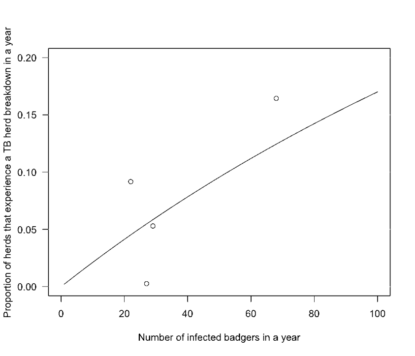
A plot of the proportion of herds predicted to experience a bTB herd breakdown in a single year under model 2, versus the total number of infected badgers culled () is shown in Figure 2 (based on dataset 1). Since , Figure 2 shows a positive relationship between the proportion of newly infected cattle herds in a year and the number of infected badgers culled in a year. It also shows the implications, based on the model, that a highly infected badger population would have on the infection rates of the cattle population, assuming that infection rates of the culled badgers is indicative of the infection rates of the whole badger population. As the infected badger population grows, so too will the proportion of infected herds in the population. However, the fitted model is based on only four empirical observations and that for county Cork is highly influential in the fitted model.
Based on the best model fit to data set 1, model 2, a 50% reduction in the proportion of infected badgers culled would result in a 46% reduction of bTb incidence in herds in Cork and a 48% reduction in the other three counties- Donegal, Kilkenny and Monaghan.
The results for data sets 2, 3 and 4 are very similar to those of data set 1. The best fitting model in each case is model 2, where and the estimated values for differ only slightly from that of data set 1 (data set 2: % data set 3: 95% data set 4: % The results for data set 5 from the pre-study period only are completely different from those obtained for the other four data sets, with model 8 as the best fitting model, which estimates a non-zero frequency-dependent between-herd transmission parameter (, 95 C.I.: 2.0873-2.4073) and no transmission from wildlife ().
3.2 Model Validity
3.2.1 Prediction
The parameter estimates of the best fitting model to data set 1 (i.e. and ) were applied to the next year of data (i.e. badger data from 1998/1999 and cattle data from 1997/1998) to get estimates , the number of restricted herds. Values of =16, 6, 6, 21 for the four counties respectively were obtained compared to the observed numbers of restricted herds . The lack of agreement reflects the yearly variation in herd bTB incidence in these data and large changes in the badger population due to proactive badger culling.
A question also arises as to how critical the assumed badger-to-herd infection rates are in these models, as model 8 is best for the pre-study period while model 2 is best for the study period. The fifth data set used data on badgers from the pre-study period only, when few badgers were culled. In all models, it is assumed that the number of badgers culled is equal to the badger population size and thus the badger population size is greatly underestimated for data set 5. Models were re-fitted with adjustments to the population size, to examine how results changed. Assuming and as in the first year of the study period for the data of pre-study, all models were re-fitted to this data set and the best one found i.e. and from data set 5 were used with the and from data set 1. The results for this adjusted data set 5 were similar to those for data set 1. Model 2 (and 6, 10) was the best fit with no between-herd transmission () and the badger-to-herd transmission rate is proportional to the total number of infected badgers culled, estimated as (, 95% C.I.: 0.0147-0.0182). This is higher than the estimate for data set 1 (=0, =0.0022, 95% C.I.: 0.0018-0.0026).
3.2.2 Identifiability
To check the identifiability of the models, the log-likelihood of each model, given by equation (9), was computed for a grid of and pairs and distinct values were obtained over the grid indicating identifiability was not a problem.
3.2.3 Sensitivity analysis
Table 3 shows the results of the sensitivity analysis. The table of results ranks parameters in decreasing order of standardised coefficients (i.e. S.E.) size. The standardised coefficients allow us to compare the relative importance of the six parameters. The results indicate that all six parameters are important in the model, , the total number of herds, being the most important and herd test sensitivity, , being the least. It can also be seen that the greater the rate of disease transmission from badgers, the greater the predicted number of infected cattle. The average length of time a herd spends on MC in years also influences the course of the epidemic. The longer the average length of time a herd spends on MC, the smaller the predicted number of infected cattle. Also, the greater the sensitivity of the SICTT herd test, the greater the predicted number of infected cattle, as to be expected.
In the second sensitivity analysis several parameter sets were created with (the length of time on MC), (SICTT sensitivity) and (the proportion of infected herds detected via slaughterhouse surveillance) set to their minimum and maximum likely values as indicated in Table 2 and models 1 to 11 were re-ran. For all parameter sets, the model selection and parameter estimates ( and ) remained unchanged thus indicating the robustness of the results to changes in values of the parameters , and .
4 Discussion
The study has been performed on a small set of observational data and there is very little repetition in the data since there were only four counties, thus we cannot draw conclusions from the results with great certainty. However, the herd population size in each of the four counties studied was large. Thus, within the limitations above and other study limitations described below, estimated model parameters are precise.
Five data sets were taken from the cattle and badger data from the FAP in Ireland and for four of them, the model that best fit assumed transmission from badgers to cattle was proportional to the total number of infected badgers culled and had no herd-to-herd-transmission. The assumption regarding the badger population size was critical in the differing model selection for the fifth data set. When this was adjusted and a more realistic badger population size assumed, results similar to the other data sets were obtained. These findings suggest herd-to-herd transmission is of much lesser importance for these areas than badger-to-herd transmission.
The results indicate that there is a significant association between levels of bTB in badgers and cattle. This does not prove causality but is, however, in agreement with results from the FAP and RBCT where some measure of causality was established (Griffin et al., 2005; Bourne et al., 2007). Reductions in cattle bTB incidence, due to proactive culling of badgers, ranged from 51% to 68% over a five-year culling period in the FAP and 23% in the RBCT. However, since herd bTB was not eliminated, these results also indicated there are sources of infection other than the badger.
In this model, it was assumed that there were only two possible sources of infection of cattle herds, between-herd infection and infection from wildlife, namely wild badgers, to cattle. Infection from any other wildlife, such as deer, was ignored, as was within-herd infection (i.e. cattle-to-cattle infection in a single herd). As in Barlow et al. (1998), re-infection of wildlife, in our case wild badgers, from cattle herds was also considered to be negligible and the inferences made here were conditional on any such reinfections being negligible. In addition, it was assumed that cattle infection, as shown by reaction on a skin test, was equivalent to the animal being infectious and that there is no carrier state in cattle or badgers. Issues in relation to animal testing are discussed in Clegg et al. (2011).
In human populations, one-third of the world’s population is infected, either latently or actively, with tuberculosis (Ozcaglar et al., 2012). The rate of latent infection of cattle herds in Ireland has yet to be established. Ozcaglar et al. (2012) in their simulation study, showed that a human tuberculosis epidemic can be viewed as a series of linked subepidemics: a fast tuberculosis subepidemic driven by direct progression, a slow tuberculosis subepidemic driven by endogenous reactivation, and a relapse tuberculosis subepidemic driven by relapse cases; thus, proving that young and mature tuberculosis epidemics behave differently and suggested that different control strategies may be necessary for controlling each subepidemic. Thus, the issue of latent infection of a herd is an important aspect of bTB epidemiology as this will perhaps drive a subepidemic by endogenous reactivation. A similar statement can be made in relation to wild badgers and has important implications for vaccine testing also, now underway (Aznar et al., 2011). Previous history of infection in a herd has been shown to be a risk factor for bTB in many studies (Griffin et al., 2005; Bourne et al., 2007) and this may be related to latent infection. Thus, the important aspect of epidemic modelling of latent infection with bTB needs study.
Epidemic models are particularly suitable for investigating the likelihood of persistence versus fade-out of infection. Blower et al. (1995) demonstrated that it takes several hundred years for a tuberculosis epidemic in humans to rise, fall, and reach an endemic state. Our models estimated approximate reproduction numbers of less than 1, indicating the epidemic would ultimately fade-out, although slowly. This was an asymptotic result and assumed a constant herd population size, while in fact, the herd population size in Ireland is continually changing (Kelly et al., 2008). More accurate estimates of reproduction numbers and epidemic length would require a separate simulation study. For example, Vynnycky and Fine (1998) include estimates of infection and re-infection rates over time for different ages, and include rates at which individuals who have been infected or reinfected for a time without developing disease move into the ‘latent’ class, in their models.
The models used here assumed the population of herds was closed - no immigration i.e. no recruitment. However, from the sensitivity analysis, we can conclude that bTB transmission is influenced by the herd population size i.e. the number of herds. This suggests that increases in population size as a result of economic or other policies may impact strongly on the course of the disease. The assumption of a closed herd population also implies there are no introduced cattle into any herd over the study period and no long range cattle movements. Both of these assumptions are unrealistic, particularly in the Irish context and both factors are known risk factors in herd bTB (Sheridan, 2011).
Our results are quite different to those of Donnelly and Hone (2010) that were based on data from the RBCT. They found the model that best fit the RBCT data, using a data set comparable to data set 1 here, was model 11, which has frequency-dependent between-herd transmission and badger-to-herd transmission proportional to the proportion of infected badgers culled. They found much stronger support for frequency-dependent badger-to-cattle transmission than density-dependent. Our results, based on the FAP data, suggest that there is stronger support for density-dependent badger-to-cattle transmission, with the wildlife transmission variable being the number of infected badgers culled. In a simple comparison we found that the biggest difference between the RBCT data used by Donnelly and Hone (2010) and the FAP data used here, was that the proportion of infected badgers is much higher in each of the four removal areas in the FAP than in the majority, though not all, badger proactive culling areas of the RBCT. The FAP and RBCT are alike in terms of numbers of herds per km2 and infection rates in herds.
It should also be noted that the models used here are idealised in form and in addition to the limitations described above, they do not take into account other features of the epidemic in question. For example, it is assumed the rate of badger-to-cattle herd transmission is independent of herd size and this may not be true. Herd size has been shown in many studies to be one of the most important risk factors for herd bTB (Griffin et al., 2005; Bourne et al., 2007; Kelly et al., 2008) and the sensitivity analysis above showed changes in rates of badger-to-cattle herd transmission has a dramatic effect on model results. Thus, results should be interpreted as representing transmission dynamics with transmission rates averaged over herd sizes.
Farm management practice changes, control policy changes, economic changes and climate changes may all affect the course of an epidemic and these factors require separate study. In addition spatial correlation structures related to transmission may also be important. Cowled et al. (2012) found that epidemic models for swine fever in wild pigs in Australia that do not take realistic spatial structures of the wildlife population into account may overestimate the rate at which a disease will spread and overestimate the size of an outbreak. A more detailed and complete study could be considered for the future.
However, this study does provide further evidence for the importance of the role of wild badgers on bTB levels in cattle herds in Ireland. This study also demonstrates that, unlike in Great Britain (based on the RBCT), herd-to-herd transmission of bTB is of much lesser importance.
References
- 1 Anderson, R.M., May, R.M., 1991. Infectious Diseases of Humans: Dynamics and Control, Oxford University Press, Oxford, UK.
- 2 Aznar, I., McGrath, G., Murphy, D., Corner, L.A.L., Gormley, E., Frankena, K., More, S.J., Martin, W., O’Keeffe, J., De Jong, M.C.M., 2011. Trial design to estimate the effect of vaccination on tuberculosis incidence in badgers. Veterinary Microbiology 151, 104-111.
- 3 Barlow, N. D., Kean, J. M., Caldwell, N. P., Ryan, T. J., 1998. Modelling the regional dynamics and management of bovine tuberculosis in New Zealand cattle herds. Preventive Veterinary Medicine 36, 25-38.
- 4 Blower, S.M., McLean, A.R., Porco, T.C., Small, P.M., Hopewell, P.C., Sanchez, M.A., Moss, A.R., 1995. The intrinsic transmission dynamics of tuberculosis epidemics. Nature Medicine 1, 815-821.
- 5 Bourne, F.J., Donnelly, C.A., Cox, D.R., Gettinby, G., McInerney, J.P., Morrison, W.I., Woodroffe, R., 2007. Bovine TB: the scientific evidence. A science base for a sustainable policy to control TB in cattle: final report of the independent scientific group on cattle TB. Department of Environment Food and Rural Affairs, London, UK.
- 6 Burnham, K.P., Anderson, D.R., 2002. Model selection and multimodel inference: a practical information. Theoretic Approach, 2nd ed. Springer-Verlag.
- 7 Clegg, T.A., Duignan, A., Whelan, C., Gormley, E., Good, M., Clarke, J., Toft, N., More, S.J., 2011. Using latent class analysis to estimate the test characteristics of the interferon- test, the single intradermal comparative tuberculin test and a multiplex immunoassay under Irish conditions. Veterinary Microbiology. DOI:10.1016/j.vetmic.2011.02.027.
- 8 Corner, L.A.L., Clegg, T.A., More, S.J., Williams, D.H., O’Boyle, I., Costello, E., Sleeman, D.P., Griffin, J.M., 2008. The effect of varying levels of population control on the prevalence of tuberculosis in badgers in Ireland. Research in Veterinary Science 85, 238 - 249.
- 9 Cowled, B.D., Garner, M.G., Negus, K., Ward, M.P., 2012. Controlling disease outbreaks in wildlife using limited culling: modelling classical swine fever incursions in wild pigs in Australia. Veterinary Research 43, 1-16.
- 10 Cox, D.R., Donnelly, C.A., Bourne, F.J., Gettinby, G., McInerney, J.P., Morrison, W.I., Woodroffe, R., 2005. Simple model for tuberculosis in cattle and badgers. Proceedings of the National Academy of Sciences 102, 17588-17593.
- 11 Cross, P.C., Getz, W.M, 2006. Assessing vaccination as a control strategy in an ongoing epidemic: Bovine tuberculosis in African buffalo. Ecological Modelling 196, 494-504.
- 12 DAFF, 1996. Department of Agriculture Food and Forestry, Badger Manual. DAFF, Ireland.
- 13 De Jong, M.C.M., 1995. Mathematical modelling in veterinary epidemiology: why model building is important. Preventive Veterinary Medicine 25, 183-193.
- 14 Donnelly, C.A., Hone, J., 2010. Is there an association between levels of bovine tuberculosis in cattle herds and badgers? Statistical Communications in Infectious Diseases 2. DOI: 10.2202/1948-4690.1000
- 15 Frankena, K., White, P.W., Keeffe, O., Costello, E., Martin, S.W., van Grevenhof, E.M., More, S.J., 2007. Quantification of the relative efficiency of factory surveillance in the disclosure of tuberculosis lesions in attested Irish cattle. Veterinary Record 161, 676-684.
- 16 Green, L.E., Medley, G.F., 2002. Mathematical modelling of the foot and mouth disease epidemic of 2001: strengths and weaknesses. Research in Veterinary Science 73, 201-205.
- 17 Griffin, J.M., Williams, D.H., Kelly, G.E., Clegg, T.A., O’Boyle, I., Collins, J.D., More, S.J., 2005. The impact of badger removal on the control of tuberculosis in cattle herds in Ireland. Preventive Veterinary Medicine 67, 237-266.
- 18 Judge, J., Ward, A., Delahay, R., McDonald, R., Roper, T., Tolhurst, B., Garnett, B., 2009. Tracking badger visits to farmyards. Comment on: Incidence of visits by badgers to farmyards in Ireland in winter. Veterinary Record 164, 667-668.
- 19 Kelly, G.E., Condon, J., More, S.J., Dolan, L., Higgins, I., Eves, J., 2008. A long term observational study of the impact of badger removal on herd restrictions due to bovine TB in the Irish midlands during 1989-2004. Epidemiolgy and Infection 136, 1362-1373.
- 20 Kelly, G.E., McGrath, G.E., More S.J., 2010. Estimating the extent of spatial association of Mycobacterium bovis infection in badgers in Ireland. Epidemiology and Infection 138, 270-279.
- 21 Ozcaglar, C., Shabbeer, A., Vandenberg, S.L., Yener, B., Bennett, K.P., 2012. Epidemiological models of Mycobacterium tuberculosis complex infections. Mathematical Biosciences 236, 77-96.
- 22 O’Meara, D.B., Edwards, C.J., Sleeman, D.P., Cross, T.F., Statham, M.J., McDowell, J.R., Dillane, E., Coughlan, J.P., O’Leary, D., O’Reilly, C., Bradley, D.G., Carlsson, J., 2012. Genetic structure of Eurasian badgers Meles meles (Carnivora: Mustelidae) and the colonization history of Ireland. Biological Journal of the Linnean Society 106, 893-909.
- 23 Sheridan, M, 2011. Progress in tuberculosis eradication in Ireland. Veterinary Microbiology, 151, 160-169.
- 24 Sleeman, D.P., Davenport, J., Fitzgerald, A., 2008. Incidence of visits by badgers to farmyards in Ireland in winter. Veterinary Record 163, 724.
- 25 Vynnycky, E., Fine, P.E.M., 1998. The long-term dynamics of tuberculosis and other diseases with long serial intervals: implications of and for changing reproduction numbers. Epidemiology and Infection 121, 309-324.
- 26 White, L.J., Evans, N.D., Lam, T.J., Schukken, Y.H., Medley, G.F., Godfrey, K.R., Chappell, M.J., 2001. The structural identifiability and parameter estimation of a multispecies model for the transmission of mastitis in diary cows. Mathematical Biosciences 174, 77-90.
| Area |
Total Herds
(N) |
Total Herds Restricted (B) |
Total Badgers
Culled
(N) |
Total Infected
Badgers Culled (I) |
| Data set 1 | ||||
| Cork | 292 | 48 | 235 | 68 |
| Donegal | 379 | 1 | 190 | 27 |
| Kilkenny | 229 | 21 | 188 | 22 |
| Monaghan | 680 | 36 | 165 | 29 |
| Data set 2 | ||||
| Cork | 288 | 29 | 235 | 68 |
| Donegal | 375 | 3 | 190 | 27 |
| Kilkenny | 230 | 14 | 188 | 22 |
| Monaghan | 687 | 19 | 165 | 29 |
| Data set 3 | ||||
| Cork | 288 | 67 | 446 | 115 |
| Donegal | 375 | 14 | 273 | 40 |
| Kilkenny | 230 | 34 | 409 | 56 |
| Monaghan | 701 | 112 | 414 | 66 |
| Data set 4 | ||||
| Cork | 294 | 230 | 467 | 116 |
| Donegal | 396 | 87 | 282 | 44 |
| Kilkenny | 233 | 119 | 618 | 107 |
| Monaghan | 701 | 338 | 627 | 88 |
| Data set 5 | ||||
| Cork | 294 | 163 | 21 | 1 |
| Donegal | 396 | 73 | 9 | 4 |
| Kilkenny | 233 | 85 | 209 | 51 |
| Monaghan | 680 | 226 | 213 | 22 |
| Parameter | Symbol | Minimum | Maximum | Source |
|---|---|---|---|---|
| Total number of herds | 200 | 1,000 | From data in this paper | |
| Average length of time a herd spends on MC in years | 0.329 | 0.7 | M. Good, DAFM, personal communication & Donnelly and Hone (2010) | |
| Herd test sensitivity rate in per cent | 0.529 | 0.606 | Clegg et al. (2011) | |
| Rate of infected cattle detection through slaughterhouse surveillance per annum | 0.27 | 0.46 | Frankena et al. (2007) | |
| Proportionality constant associated with the rate of infection from wildlife | 0 | 0.8 | From data in this paper | |
| Total number of infected badgers culled | 10 | 100 | From data in this paper |
[b]
| Parameter1 | Symbol | Coefficient () 2 | Standard Error (S.E.) | S.E. |
|---|---|---|---|---|
| Total number of herds | 412.26 | 0.39 | 1051.68 | |
| Proportionality constant associated with the rate of infection from wildlife | 95.51 | 0.23 | 412.92 | |
| Rate of infected cattle detection through slaughterhouse surveillance per annum | 126.74 | 0.95 | 133.75 | |
| Total number of infected badgers culled | 32.76 | 0.27 | 119.96 | |
| Average length of time a herd spends on MC in years | -143.01 | 1.49 | -95.75 | |
| Herd test sensitivity rate in per cent | 317.2 | 4.34 | 73.05 |
- 1
All parameters were transformed to percentage difference from the mean (i.e. , where is the value of the parameter on run and is the mean from all runs).
- 2
All coefficients have a p-value less than 0.001.
Parameter estimates and log-likelihood values from the eleven
varying models fitted to data set 1 (see Table 1) on bovine tuberculosis in cattle and
badgers from the Four Area Project. Each of the models represents some combination of the two fitted parameters
and , where is a measure of herd-to-herd transmission per annum (Density Dependent (DD) or Frequency Dependent (FD)) and is a measure of badger-to-herd transmission per annum, such that , or , where equals the number of badgers culled in an area and equals the number of infected badgers culled in an area. Model 2, highlighted in dark grey, has the
most support from the data with an Akaike weight of 0.52.
Model
Between-herd
transmission
Transmission from
wildlife11
1
: proportional to.
Number
of
parameters
p-value
p-value
Log-
likelihood
AICc22
2
AICc: Akaike Information Criterion corrected for small sample sizes
relative to the number of parameters.
Akaike
weight
1
None
1
- -33
3
In the case when we assume one of the transmission parameters,
or , is zero, we omit the parameters estimate and no p-value is
calculable.
- -33
3
In the case when we assume one of the transmission parameters,
or , is zero, we omit the parameters estimate and no p-value is
calculable.
0.0004
N/A44
4
When we assume one of the transmission parameters, or
, is zero, the calculation of the p-value of the other transmission
parameter is not applicable (N/A) since the null hypothesis would state that both
parameters were zero and hence, there would be no transmission of tuberculosis to
cattle.
-382.4703
766.94
0.000
2
None
1
- -33
3
In the case when we assume one of the transmission parameters,
or , is zero, we omit the parameters estimate and no p-value is
calculable.
-
-33
3
In the case when we assume one of the transmission parameters,
or , is zero, we omit the parameters estimate and no p-value is
calculable.
0.0022
N/A44
4
When we assume one of the transmission parameters, or
, is zero, the calculation of the p-value of the other transmission
parameter is not applicable (N/A) since the null hypothesis would state that both
parameters were zero and hence, there would be no transmission of tuberculosis to
cattle.
-372.4763
746.96
0.520
3
None
1
- -33
3
In the case when we assume one of the transmission parameters,
or , is zero, we omit the parameters estimate and no p-value is
calculable.
- -33
3
In the case when we assume one of the transmission parameters,
or , is zero, we omit the parameters estimate and no p-value is
calculable.
0.4162
N/A44
4
When we assume one of the transmission parameters, or
, is zero, the calculation of the p-value of the other transmission
parameter is not applicable (N/A) since the null hypothesis would state that both
parameters were zero and hence, there would be no transmission of tuberculosis to
cattle.
-376.2648
754.53
0.012
4
DD
None
1
0.0006
N/A44
4
When we assume one of the transmission parameters, or
, is zero, the calculation of the p-value of the other transmission
parameter is not applicable (N/A) since the null hypothesis would state that both
parameters were zero and hence, there would be no transmission of tuberculosis to
cattle.
- -33
3
In the case when we assume one of the transmission parameters,
or , is zero, we omit the parameters estimate and no p-value is
calculable.
-
-33
3
In the case when we assume one of the transmission parameters,
or , is zero, we omit the parameters estimate and no p-value is
calculable.
-752.6828
1507.39
0.000
5
DD
2
0.0000
0.942
0.0004
0.001
-380.3202
764.65
0.000
6
DD
2
0.0000
0.968
0.0022
0.001
-372.2951
748.60
0.229
7
DD
2
0.0000
0.978
0.4098
0.001
-376.1010
756.21
0.005
8
FD
None
1
1.3703
N/A44
4
When we assume one of the transmission parameters, or
, is zero, the calculation of the p-value of the other transmission
parameter is not applicable (N/A) since the null hypothesis would state that both
parameters were zero and hence, there would be no transmission of tuberculosis to
cattle.
- -33
3
In the case when we assume one of the transmission parameters,
or , is zero, we omit the parameters estimate and no p-value is
calculable.
-
-33
3
In the case when we assume one of the transmission parameters,
or , is zero, we omit the parameters estimate and no p-value is
calculable.
-388.7466
779.50
0.000
9
FD
2
0.0000
0.999
0.0004
0.001
-382.3800
768.77
0.000
10
FD
2
0.0000
0.993
0.0022
0.001
-372.2950
748.60
0.229
11
FD
2
0.0000
0.994
0.4101
0.001
-376.1002
756.21
0.005