跳到论文正文
W Papers独立论文阅读器 arXiv:2007.06365 论文正文 计算阅读时间 · 0%
引用这篇论文根据当前论文元数据生成,正式投稿前建议核对。


License: arXiv.org perpetual non-exclusive license
arXiv:2007.06365v1 [math.CO] 13 Jul 2020

Relations between the properties of a complete rooted tree and the properties of a distribution of lengths of randomly generated strings

Yurii Lahodiuk Email: yura.lagodiuk@gmail.com
Abstract

In scope of this paper we show that there are relations between the properties of a complete mm-ary rooted tree of height nn and the expectation and variance of the distribution of lengths of random strings generated from the alphabet {α1,α2,…​αm}\{\alpha_{1},\alpha_{2},\dots\alpha_{m}\} until we see nn instances of a specific symbol in a row. Based on this we demonstrate a new interpretation for the integer sequence A286778.

Overview

Consider a complete mm-ary rooted tree graph of height nn: Gm,n=(V,E)G_{m,n}=(V,E). Let’s denote the total number of edges in such tree as Tm,n:=|E|=m⋅mn−1m−1T_{m,n}:=|E|=m\cdot{m^{n}-1\over m-1}. For every node v∈Vv\in V there always exists a unique path π⁡(v)\pi(v) from the node vv to the root node (we treat paths as sets of edges). For any pair of nodes (a,b)∈V×V(a,b)\in V\times V we can find the length of the common sub-path to the root node: |π⁡(a)∩π⁡(b)||\pi(a)\cap\pi(b)|. Let’s denote the sum of the common sub-path lengths over all 2-tuples of nodes of such tree as Sm,n:=∑(a,b)∈V×V|π⁡(a)∩π⁡(b)|S_{m,n}:=\sum_{(a,b)\in V\times V}|\pi(a)\cap\pi(b)|.

Refer to caption
(a) T2,2=6T_{2,2}=6 and S2,2=22S_{2,2}=22.
Refer to caption
(b) T3,2=12T_{3,2}=12 and S3,2=57S_{3,2}=57
Figure 1: Examples of the trees and the corresponding values of Tm,nT_{m,n} and Sm,nS_{m,n}.

On the other hand, consider a process that generates a random string as follows: starting from the empty string we pick a random symbol from the alphabet {α1,α2,…​αm}\{\alpha_{1},\alpha_{2},\dots\alpha_{m}\} and append it to the string, the process continues until we see nn instances of a specific symbol (say, α1\alpha_{1}) in a row. Let’s introduce a random variable ξm,n\xi_{m,n} that represents a length of the string generated by the described process.

We will prove that the following relations between Tm,nT_{m,n} and the expectation of ξm,n\xi_{m,n}, and between Sm,nS_{m,n} and the variance of ξm,n\xi_{m,n}, are true for all m,n≥1m,n\geq 1:

Var⁡[ξm,n]=(m−1)⋅Sm,n\mathrm{Var}[\xi_{m,n}]=(m-1)\cdot S_{m,n} (1)
𝔼⁡[ξm,n]=Tm,n\mathbb{E}[\xi_{m,n}]=T_{m,n} (2)

In the table 1 you can see few examples:

(m,n) Tm,nT_{m,n} 𝔼⁡[ξm,n]\mathbb{E}[\xi_{m,n}] Sm,nS_{m,n} Var⁡[ξm,n]\mathrm{Var}[\xi_{m,n}]
(2,2) 6 6 22 22
(2,3) 14 14 142 142
(2,4) 30 30 734 734
(2,5) 62 62 3390 3390
(3,2) 12 12 57 114
(3,3) 39 39 678 1356
(3,4) 120 120 6834 13668
(4,2) 20 20 116 348
(4,3) 84 84 2228 6684
(4,4) 340 340 37812 113436
Table 1: Note, that the relations between the items in the rows obey the equations (1) and (2).

For proving the relations (1) and (2) in case when m≥2m\geq 2 we will use the closed-form expressions for Tm,nT_{m,n}, 𝔼⁡[ξm,n]\mathbb{E}[\xi_{m,n}], Sm,nS_{m,n} and Var⁡[ξm,n]\mathrm{Var}[\xi_{m,n}].

The computation of expectation 𝔼⁡[ξm,n]\mathbb{E}[\xi_{m,n}] and variance Var⁡[ξm,n]\mathrm{Var}[\xi_{m,n}] is described in the literature, for instance: the approach based on generating functions is described in [1], and the approach based on martingales is described in [2], also the closed-form expression for 𝔼⁡[ξm,n]\mathbb{E}[\xi_{m,n}] is provided in [3].

For completeness, in scope of these notes we will derive the closed-form expressions for 𝔼⁡[ξm,n]\mathbb{E}[\xi_{m,n}] and Var⁡[ξm,n]\mathrm{Var}[\xi_{m,n}]. We will use the transfer matrix method [4], which is similar to the approach based on the absorbing Markov chain. In the section 1 we will construct a matrix WW based on the adjacency matrix of a digraph that corresponds to the described string-generation problem. Using the fact, that the spectral radius of WW is less than 11 (which we will prove in the section 4) we will derive the matrix-form expressions for computing the expectation and variance (where 𝕀\mathbb{I} is an identity matrix):

𝔼⁡[ξm,n]=(0,…,0,1)⋅W⋅(𝕀−W)−2⋅(1,0,…,0)𝖳\begin{split}\mathbb{E}[\xi_{m,n}]=(0,\dots,0,1)\cdot W\cdot(\mathbb{I}-W)^{-2}\cdot(1,0,\dots,0)^{\mathsf{T}}\end{split} (3)
Var⁡[ξm,n]=(0,…,0,1)⋅W⋅(𝕀+W)⋅(𝕀−W)−3⋅(1,0,…,0)𝖳−𝔼​[ξm,n]2\begin{split}\mathrm{Var}[\xi_{m,n}]=(0,\dots,0,1)\cdot W\cdot(\mathbb{I}+W)\cdot(\mathbb{I}-W)^{-3}\cdot(1,0,\dots,0)^{\mathsf{T}}-\mathbb{E}[\xi_{m,n}]^{2}\end{split} (4)

Afterwards (in the section 2), taking into account relations between the entries of the matrices WW, (𝕀+W)(\mathbb{I}+W), and (𝕀−W)−1(\mathbb{I}-W)^{-1}, we will derive from the equations (3) and (4) the closed-form expressions for expectation and variance:

𝔼⁡[ξm,n]=m⋅mn−1m−1\begin{split}\mathbb{E}[\xi_{m,n}]=m\cdot{m^{n}-1\over m-1}\end{split} (5)
Var⁡[ξm,n]=m(m−1)2⋅(m2​n+1−(2​n+1)⋅mn+1+(2​n+1)⋅mn−1)\begin{split}\mathrm{Var}[\xi_{m,n}]&={m\over(m-1)^{2}}\cdot(m^{2n+1}-(2n+1)\cdot m^{n+1}+(2n+1)\cdot m^{n}-1)\end{split} (6)

In the section 3 we will derive the closed-form expression for Sm,nS_{m,n} using the combinatorial counting techniques:

Sm,n=m(m−1)3⋅(m2​n+1−(2​n+1)⋅mn+1+(2​n+1)⋅mn−1)\begin{split}S_{m,n}&={m\over(m-1)^{3}}\cdot(m^{2n+1}-(2n+1)\cdot m^{n+1}+(2n+1)\cdot m^{n}-1)\end{split} (7)

The equation (1) follows from the equations (6) and (7). And the equation (2) follows from the equation (5) and the definition of Tm,nT_{m,n}.

In case when m=2m=2 we have 𝔼⁡[ξ2,n]=T2,n\mathbb{E}[\xi_{2,n}]=T_{2,n} and Var⁡[ξ2,n]=S2,n\mathrm{Var}[\xi_{2,n}]=S_{2,n} for all n≥1n\geq 1. While it is known that both 𝔼⁡[ξ2,n]\mathbb{E}[\xi_{2,n}] and T2,nT_{2,n} are described by the integer sequence A000918 [5], and it is known that S2,nS_{2,n} is described by the integer sequence A286778 [6], we obtain a new interpretation for the integer sequence A286778: this sequence describes Var⁡[ξ2,n]\mathrm{Var}[\xi_{2,n}] – a variance of the number of tosses of a fair coin until we see nn heads in a row. In this case we can derive from the equation (6) the same formula as provided in [6] for computing the values of A286778:

an=4⋅22​n−(4​n+2)⋅2n−2a_{n}=4\cdot 2^{2n}-(4n+2)\cdot 2^{n}-2 (8)

As a closing remark, it worth to admit, that it might be interesting to investigate further: whether it is possible to find similar relations for the distributions of lengths of randomly generated strings, that are generated until we observe any particular (given in advance) word for the given alphabet.

1 Expectation and variance of the lengths of generated strings

In case if m=1m=1 (the alphabet contains only one symbol) the expressions for expectation and variance are trivial: 𝔼⁡[ξ1,n]=n\mathbb{E}[\xi_{1,n}]=n and Var⁡[ξ1,n]=0\mathrm{Var}[\xi_{1,n}]=0 (and the equations (1) and (2) are true in this case), so in the remaining part of the paper we will focus on the case when m≥2m\geq 2.

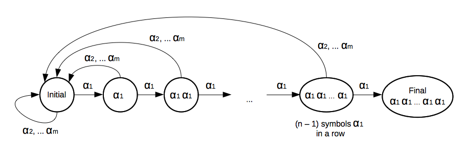
We can represent our string generation problem as a walk in the digraph displayed in the figure 2 (each edge is associated with a subset of symbols from our alphabet: either {α2,…​αm}\{\alpha_{2},\dots\alpha_{m}\}, or {α1}\{\alpha_{1}\}).

Refer to caption
Figure 2: After choosing the random symbol from the alphabet we follow the edge, which contains the chosen symbol (we start from the “initial” vertex).

This graph has a (n+1)×(n+1)(n+1)\times(n+1) adjacency matrix (9), where the outgoing edges of vertices are represented as column-vectors, and the values of the items of this matrix represent the sizes of the subsets of symbols associated with the corresponding edges.

A=I​n​i​t​i​a​lα1α1​α1…α1​α1​…​α1F​i​n​a​l(m−1)(m−1)(m−1)…(m−1)0I​n​i​t​i​a​l10……00α1010…⋮⋮α1​α1⋮⋱⋱⋱⋮⋮⋮⋮⋱⋱0⋮α1​α1​…​α10……010F​i​n​a​lA=\begin{array}[]{ccccccc}Initial&\alpha_{1}&\alpha_{1}\alpha_{1}&\dots&\alpha_{1}\alpha_{1}...\alpha_{1}&Final\\ \\ (m-1)&(m-1)&(m-1)&\dots&(m-1)&0&Initial\\ \\ 1&0&\dots&\dots&0&0&\alpha_{1}\\ \\ 0&1&0&\dots&\vdots&\vdots&\alpha_{1}\alpha_{1}\\ \\ \vdots&\ddots&\ddots&\ddots&\vdots&\vdots&\vdots\\ \\ \vdots&&\ddots&\ddots&0&\vdots&\alpha_{1}\alpha_{1}...\alpha_{1}\\ \\ 0&\dots&\dots&0&1&0&Final\\ \\ \end{array} (9)

We are interested in the number of walks, that arrive into the final vertex after kk steps (starting from the initial vertex). The matrix AkA^{k} allows to obtain the number of walks of length kk between any pair of vertices. So, the number of walks between the initial vertex and between the final vertex is a leftmost bottom element of AkA^{k}:

(0,…,0,1)⋅Ak⋅(1,0,…,0)𝖳(0,\dots,0,1)\cdot A^{k}\cdot(1,0,\dots,0)^{\mathsf{T}} (10)

Given the alphabet size mm the total number of walks of length kk is mkm^{k}, therefore the probability that the random walk of the length kk will finish in the final vertex is:

pk=1mk⋅(0,…,0,1)⋅Ak⋅(1,0,…,0)𝖳=(0,…,0,1)⋅(1m⋅A)k⋅(1,0,…,0)𝖳\begin{split}p_{k}&={1\over m^{k}}\cdot(0,\dots,0,1)\cdot A^{k}\cdot(1,0,\dots,0)^{\mathsf{T}}\\ &=(0,\dots,0,1)\cdot\left({1\over m}\cdot A\right)^{k}\cdot(1,0,\dots,0)^{\mathsf{T}}\end{split} (11)

Let’s denote W:=1m⋅AW:={1\over m}\cdot A. Also, let’s introduce a discrete random variable ξm,n\xi_{m,n}, that represents a length of the string, generated until we observed nn symbols α1\alpha_{1} in a row (ξm,n\xi_{m,n} takes values from the set {0,1,2,3,…}\{0,1,2,3,\dots\}). Thus, the expected length of the string is:

𝔼⁡[ξm,n]=∑k=0∞k⋅pk=(0,…,0,1)⋅(∑k=0∞k⋅Wk)⋅(1,0,…,0)𝖳\mathbb{E}[\xi_{m,n}]=\sum_{k=0}^{\infty}k\cdot p_{k}=(0,\dots,0,1)\cdot\left(\sum_{k=0}^{\infty}k\cdot W^{k}\right)\cdot(1,0,\dots,0)^{\mathsf{T}} (12)

In the section 4 we will investigate the spectral radius of WW, and we will show that ρ⁡(W)<1\rho(W)<1. Thus, we deal with the Neumann series: ∑k=0∞Wk=(𝕀−W)−1\sum_{k=0}^{\infty}W^{k}=(\mathbb{I}-W)^{-1}. Consequently, we can transform the infinite sum in equation (12) using the same technique as with formal power series:

∑k=0∞k⋅xk=x⋅dd​x​(∑k=0∞xk)=x(1−x)2\sum_{k=0}^{\infty}k\cdot x^{k}=x\cdot{d\over dx}\left(\sum_{k=0}^{\infty}x^{k}\right)={x\over(1-x)^{2}} (13)

Hence, the expectation can be expressed as:

𝔼⁡[ξm,n]=(0,…,0,1)⋅W⋅((𝕀−W)−1)2⋅(1,0,…,0)𝖳\mathbb{E}[\xi_{m,n}]=(0,\dots,0,1)\cdot W\cdot\left((\mathbb{I}-W)^{-1}\right)^{2}\cdot(1,0,\dots,0)^{\mathsf{T}} (14)

The product of matrices W⋅(𝕀−W)−1W\cdot(\mathbb{I}-W)^{-1} is commutative (the proof is in the section 6), so the order of matrices in the equation (14) does not matter.

Now, let’s compute the variance:

Var⁡[ξm,n]=𝔼⁡[ξm,n2]−𝔼​[ξm,n]2\mathrm{Var}[\xi_{m,n}]=\mathbb{E}[\xi_{m,n}^{2}]-\mathbb{E}[\xi_{m,n}]^{2} (15)

Let’s compute 𝔼⁡[ξm,n2]\mathbb{E}[\xi_{m,n}^{2}]:

𝔼⁡[ξm,n2]=∑k=0∞k2⋅pk=(0,…,0,1)⋅(∑k=0∞k2⋅Wk)⋅(1,0,…,0)𝖳\mathbb{E}[\xi_{m,n}^{2}]=\sum_{k=0}^{\infty}k^{2}\cdot p_{k}=(0,\dots,0,1)\cdot\left(\sum_{k=0}^{\infty}k^{2}\cdot W^{k}\right)\cdot(1,0,\dots,0)^{\mathsf{T}} (16)

As far as ρ⁡(W)<1\rho(W)<1, we can transform the sum ∑k=0∞k2⋅Wk\sum_{k=0}^{\infty}k^{2}\cdot W^{k} using the same technique as with formal power series:

∑k=0∞k2⋅xk=x⋅dd​x​(∑k=0∞k⋅xk)=x⋅(1+x)(1−x)3\sum_{k=0}^{\infty}k^{2}\cdot x^{k}=x\cdot{d\over dx}\left(\sum_{k=0}^{\infty}k\cdot x^{k}\right)={x\cdot(1+x)\over(1-x)^{3}} (17)

Hence, 𝔼⁡[ξm,n2]\mathbb{E}[\xi_{m,n}^{2}] could be expressed as:

𝔼⁡[ξm,n2]=(0,…,0,1)⋅W⋅(𝕀+W)⋅((𝕀−W)−1)3⋅(1,0,…,0)𝖳\mathbb{E}[\xi_{m,n}^{2}]=(0,\dots,0,1)\cdot W\cdot(\mathbb{I}+W)\cdot\left((\mathbb{I}-W)^{-1}\right)^{3}\cdot(1,0,\dots,0)^{\mathsf{T}} (18)

The products of matrices W⋅(𝕀+W)W\cdot(\mathbb{I}+W) and (𝕀+W)⋅(𝕀−W)−1(\mathbb{I}+W)\cdot(\mathbb{I}-W)^{-1} are commutative (the proof is in the section 6), so the order of matrices in the equation (18) does not matter.

From equations (14) and (18) we obtain the matrix-form expression for the variance:

Var⁡[ξm,n]=𝔼⁡[ξm,n2]−𝔼​[ξm,n]2=(0,…,0,1)⋅W⋅(𝕀+W)⋅((𝕀−W)−1)3⋅(1,0,…,0)𝖳−−((0,…,0,1)⋅W⋅((𝕀−W)−1)2⋅(1,0,…,0)𝖳)2\begin{split}\mathrm{Var}[\xi_{m,n}]=&\mathbb{E}[\xi_{m,n}^{2}]-\mathbb{E}[\xi_{m,n}]^{2}\\ =&(0,\dots,0,1)\cdot W\cdot(\mathbb{I}+W)\cdot\left((\mathbb{I}-W)^{-1}\right)^{3}\cdot(1,0,\dots,0)^{\mathsf{T}}-\\ &-\left((0,\dots,0,1)\cdot W\cdot\left((\mathbb{I}-W)^{-1}\right)^{2}\cdot(1,0,\dots,0)^{\mathsf{T}}\right)^{2}\\ \end{split} (19)

Generally speaking, for the cases when we generate random strings until we encounter any arbitrary word constructed from the given alphabet (not only until we see nn instances of a specific symbol in a row) – the matrix-form expressions for expectation and variance (14) and (19) are true as long as the series, that involve the corresponding matrix WW, converges. But, still, in scope of this paper we focus on the random string generation process that continues until we see nn instances of a specific symbol in a row.

2 The closed-form expressions for expectation and variance

Taking into account the structure of the matrix AA from the equation (9) and that W:=1m⋅AW:={1\over m}\cdot A, we can notice that the values of entries of the matrix (𝕀−W)−1(\mathbb{I}-W)^{-1} obey a simple pattern:

mn(mn−m1)(mn−m2)…(mn−mk)…(mn−mn)⋮mn−1(mn−1−m1)…(mn−1−mk−1)…⋮⋮⋮mn−2…⋮…⋮⋮⋮⋮⋮⋮⋮⋮⋮⋱(mn−k+1−m1)⋮⋮⋮⋮mn−k⋮⋮⋮⋮⋮⋮m2m2m2…m2(m2−m2)m1m1m1…m1⋱(m1−m1)m0m0m0…m0…m0\begin{array}[]{cccccccc}\\ m^{n}&(m^{n}-m^{1})&(m^{n}-m^{2})&\dots&(m^{n}-m^{k})&\dots&(m^{n}-m^{n})\\ \vdots&m^{n-1}&(m^{n-1}-m^{1})&\dots&(m^{n-1}-m^{k-1})&\dots&\vdots\\ \vdots&\vdots&m^{n-2}&\dots&\vdots&\dots&\vdots\\ \vdots&\vdots&\vdots&&\vdots&&\vdots\\ \vdots&\vdots&\vdots&\ddots&(m^{n-k+1}-m^{1})&&\vdots\\ \vdots&\vdots&\vdots&&m^{n-k}&&\vdots\\ \vdots&\vdots&\vdots&&\vdots&&\vdots\\ m^{2}&m^{2}&m^{2}&\dots&m^{2}&&(m^{2}-m^{2})\\ m^{1}&m^{1}&m^{1}&\dots&m^{1}&\ddots&(m^{1}-m^{1})\\ m^{0}&m^{0}&m^{0}&\dots&m^{0}&\dots&m^{0}\\ \\ \end{array} (20)

Considering the structure of the matrix WW we can compute (0,…,0,1)⋅W(0,\dots,0,1)\cdot W:

(0,…,0,0,1)⋅W=(0,…,0,1m,0)(0,\dots,0,0,1)\cdot W=\left(0,\dots,0,{1\over m},0\right) (21)

Let’s compute (𝕀−W)−1⋅(1,0,…,0)𝖳(\mathbb{I}-W)^{-1}\cdot(1,0,\dots,0)^{\mathsf{T}} using the matrix from (20):

(𝕀−W)−1⋅(1,0,…,0)𝖳=(mn,mn−1,mn−2,…,m0)𝖳(\mathbb{I}-W)^{-1}\cdot(1,0,\dots,0)^{\mathsf{T}}=(m^{n},m^{n-1},m^{n-2},\dots,m^{0})^{\mathsf{T}} (22)

Using the similar vector-matrix multiplications as in (21) and (22) we can compute the closed-form expression for 𝔼⁡[ξm,n]\mathbb{E}[\xi_{m,n}]:

𝔼⁡[ξm,n]=(0,…,0,1)⋅W⋅((𝕀−W)−1)2⋅(1,0,…,0)𝖳=(0,…,0,1m,0)⋅(𝕀−W)−1⋅(mn,mn−1,mn−2,…,m0)𝖳=((0,…,0,1m,0)⋅(𝕀−W)−1)⋅(mn,mn−1,mn−2,…,m0)𝖳=(1m⋅(m,m,m,…,m,0))⋅(mn,mn−1,mn−2,…,m0)𝖳=(1,…,1,0)⋅(mn,mn−1,mn−2,…,m0)𝖳=∑k=1nmk=m⋅(mn−1)(m−1)\begin{split}\mathbb{E}[\xi_{m,n}]&=(0,\dots,0,1)\cdot W\cdot\left((\mathbb{I}-W)^{-1}\right)^{2}\cdot(1,0,\dots,0)^{\mathsf{T}}\\ &=\left(0,\dots,0,{1\over m},0\right)\cdot(\mathbb{I}-W)^{-1}\cdot(m^{n},m^{n-1},m^{n-2},\dots,m^{0})^{\mathsf{T}}\\ &=\left(\left(0,\dots,0,{1\over m},0\right)\cdot(\mathbb{I}-W)^{-1}\right)\cdot(m^{n},m^{n-1},m^{n-2},\dots,m^{0})^{\mathsf{T}}\\ &=\left({1\over m}\cdot(m,m,m,\dots,m,0)\right)\cdot(m^{n},m^{n-1},m^{n-2},\dots,m^{0})^{\mathsf{T}}\\ &=(1,\dots,1,0)\cdot(m^{n},m^{n-1},m^{n-2},\dots,m^{0})^{\mathsf{T}}\\ &=\sum_{k=1}^{n}m^{k}=m\cdot{(m^{n}-1)\over(m-1)}\end{split} (23)

So, we have shown that 𝔼⁡[ξm,n]=m⋅(mn−1)(m−1)\mathbb{E}[\xi_{m,n}]=m\cdot{(m^{n}-1)\over(m-1)}.

Now, let’s compute 𝔼⁡[ξm,n2]\mathbb{E}[\xi_{m,n}^{2}]:

𝔼⁡[ξm,n2]=(0,…,0,1)⋅W⋅(𝕀+W)⋅((𝕀−W)−1)3⋅(1,0,…,0)𝖳=(0,…,0,1m,0)⋅(𝕀+W)⋅((𝕀−W)−1)2⋅(mn,mn−1,mn−2,…,m0)𝖳=((0,…,0,1m,0)⋅(𝕀+W))⋅((𝕀−W)−1)2⋅(mn,mn−1,mn−2,…,m0)𝖳=(0,…,0,1m2,1m,0)⋅((𝕀−W)−1)2⋅(mn,mn−1,mn−2,…,m0)𝖳=((0,…,0,1m2,1m,0)⋅(𝕀−W)−1)⋅(𝕀−W)−1⋅(mn,mn−1,mn−2,…,m0)𝖳=(2,…,2,2​m−1m,0)⋅(𝕀−W)−1⋅(mn,mn−1,mn−2,…,m0)𝖳=(a0,a1,…,an−1,0)⋅(mn,mn−1,mn−2,…,m0)𝖳\begin{split}\mathbb{E}[\xi_{m,n}^{2}]&=(0,\dots,0,1)\cdot W\cdot(\mathbb{I}+W)\cdot\left((\mathbb{I}-W)^{-1}\right)^{3}\cdot(1,0,\dots,0)^{\mathsf{T}}\\ &=\left(0,\dots,0,{1\over m},0\right)\cdot(\mathbb{I}+W)\cdot\left((\mathbb{I}-W)^{-1}\right)^{2}\cdot(m^{n},m^{n-1},m^{n-2},\dots,m^{0})^{\mathsf{T}}\\ &=\left(\left(0,\dots,0,{1\over m},0\right)\cdot(\mathbb{I}+W)\right)\cdot\left((\mathbb{I}-W)^{-1}\right)^{2}\cdot(m^{n},m^{n-1},m^{n-2},\dots,m^{0})^{\mathsf{T}}\\ &=\left(0,\dots,0,{1\over m^{2}},{1\over m},0\right)\cdot\left((\mathbb{I}-W)^{-1}\right)^{2}\cdot(m^{n},m^{n-1},m^{n-2},\dots,m^{0})^{\mathsf{T}}\\ &=\left(\left(0,\dots,0,{1\over m^{2}},{1\over m},0\right)\cdot(\mathbb{I}-W)^{-1}\right)\cdot(\mathbb{I}-W)^{-1}\cdot(m^{n},m^{n-1},m^{n-2},\dots,m^{0})^{\mathsf{T}}\\ &=\left(2,\dots,2,{2m-1\over m},0\right)\cdot(\mathbb{I}-W)^{-1}\cdot(m^{n},m^{n-1},m^{n-2},\dots,m^{0})^{\mathsf{T}}\\ &=(a_{0},a_{1},\dots,a_{n-1},0)\cdot(m^{n},m^{n-1},m^{n-2},\dots,m^{0})^{\mathsf{T}}\end{split} (24)

Where ak=2​mm−1⋅(mn−mk)−1a_{k}={2m\over m-1}\cdot(m^{n}-m^{k})-1 for every k∈{0,1,…,n−1}k\in\{0,1,\dots,n-1\}.

Thus:

𝔼⁡[ξm,n2]=∑k=1nmk⋅an−k=∑k=1nmk⋅(2​mm−1⋅(mn−mn−k)−1)=m(m−1)2⋅(2⋅m2​n+1−(2​n+3)⋅mn+1+(2​n+1)⋅mn+m−1)\begin{split}\mathbb{E}[\xi_{m,n}^{2}]&=\sum_{k=1}^{n}m^{k}\cdot a_{n-k}\\ &=\sum_{k=1}^{n}m^{k}\cdot\left({2m\over m-1}\cdot(m^{n}-m^{n-k})-1\right)\\ &={m\over(m-1)^{2}}\cdot(2\cdot m^{2n+1}-(2n+3)\cdot m^{n+1}+(2n+1)\cdot m^{n}+m-1)\end{split} (25)

From equations (23) and (25) we can obtain the closed-form expression for variance:

Var⁡[ξm,n]=𝔼⁡[ξm,n2]−𝔼​[ξm,n]2=m(m−1)2⋅(m2​n+1−(2​n+1)⋅mn+1+(2​n+1)⋅mn−1)\begin{split}\mathrm{Var}[\xi_{m,n}]&=\mathbb{E}[\xi_{m,n}^{2}]-\mathbb{E}[\xi_{m,n}]^{2}\\ &={m\over(m-1)^{2}}\cdot(m^{2n+1}-(2n+1)\cdot m^{n+1}+(2n+1)\cdot m^{n}-1)\end{split} (26)

3 Sum of the common sub-path lengths in the complete mm-ary tree of depth nn

Given a complete mm-ary rooted tree of depth nn: Gm,n=(V,E)G_{m,n}=(V,E), we will find the closed-form expression for Sm,n:=∑(a,b)∈V×V|π⁡(a)∩π⁡(b)|S_{m,n}:=\sum_{(a,b)\in V\times V}|\pi(a)\cap\pi(b)|, where π⁡(v)\pi(v) is a set of edges that represents a path from the node v∈Vv\in V to the root node of the tree.

Consider some integer d∈{1,2,…​n}d\in\{1,2,\dots n\} which represents the length of a common sub-path. Let’s define the subset Pd⊂V×VP_{d}\subset V\times V, such that ∀(a,b)∈Pd\forall(a,b)\in P_{d}: |π⁡(a)∩π⁡(b)|=d|\pi(a)\cap\pi(b)|=d. Then:

Sm,n=∑d=1nd⋅|Pd|S_{m,n}=\sum_{d=1}^{n}d\cdot|P_{d}| (27)

Consider a pair (a,b)∈Pd(a,b)\in P_{d}. As far as the length of the common sub-path between π⁡(a)\pi(a) and π⁡(b)\pi(b) is dd, the deepest common node of these two paths (let’s call it cc) is located in the dd-th level of the tree. There are mdm^{d} nodes in the dd-th level of the tree. Hence, the set PdP_{d} can be represented as a union of mdm^{d} disjoint subsets QcQ_{c} (where QcQ_{c} represents the set of pairs (a,b)(a,b) whose paths contain a deepest common node cc, located in the dd-th level of the tree):

|Pd|=md⋅|Qc||P_{d}|=m^{d}\cdot|Q_{c}| (28)

For computing |Qc||Q_{c}| we need to consider the following three disjoint cases:

  • •

    Case 1: Nodes aa and bb are located in the different subtrees of cc (see the figure 3a). There are (m2){m\choose 2} possibilities to choose such subtrees. Each of these subtrees contains ∑k=0n−1−dmk=mn−d−1m−1\sum_{k=0}^{n-1-d}m^{k}={m^{n-d}-1\over m-1} nodes. The node aa is taken from one subtree, and the node bb is taken from the other subtree. The total number of tuples (a,b)(a,b) constructed in such case is: 2⋅(m2)⋅(mn−d−1m−1)22\cdot{m\choose 2}\cdot\left({m^{n-d}-1\over m-1}\right)^{2}.

  • •

    Case 2: One of the nodes of the tuple is cc, and the other node belongs to the subtree of cc (see the figure 3b). There are m⋅∑k=0n−1−dmk=mn−d+1−1m−1−1m\cdot\sum_{k=0}^{n-1-d}m^{k}={m^{n-d+1}-1\over m-1}-1 possibilities to choose a descendant of cc. The total number of tuples (a,b)(a,b) constructed in such case is: 2⋅(mn−d+1−1m−1−1)2\cdot\left({m^{n-d+1}-1\over m-1}-1\right).

  • •

    Case 3: Both nodes in the tuple are cc: (a,b)=(c,c)(a,b)=(c,c). There is only 11 such case.

Refer to caption
(a) Both nodes from the tuple (a,b)(a,b) are descendants of the node cc.
Refer to caption
(b) One node from the tuple (a,b)(a,b) is descendant of the node cc, and the other node from the tuple is the node cc.
Figure 3: Two cases when the length of the common sub-path is dd.

Thus, taking into account that the described cases are disjoint:

|Qc|=2⋅(m2)⋅(mn−d−1m−1)2+2⋅(mn−d+1−1m−1−1)+1|Q_{c}|=2\cdot{m\choose 2}\cdot\left({m^{n-d}-1\over m-1}\right)^{2}+2\cdot\left({m^{n-d+1}-1\over m-1}-1\right)+1 (29)

From equations (28) and (29) we have:

|Pd|=md⋅(2⋅(m2)⋅(mn−d−1m−1)2+2⋅(mn−d+1−1m−1−1)+1)|P_{d}|=m^{d}\cdot\left(2\cdot{m\choose 2}\cdot\left({m^{n-d}-1\over m-1}\right)^{2}+2\cdot\left({m^{n-d+1}-1\over m-1}-1\right)+1\right) (30)

Hence the sum of the common lengths over all 2-tuples of nodes of the complete mm-ary tree of depth nn is:

Sm,n=∑d=1nd⋅md⋅(2⋅(m2)⋅(mn−d−1m−1)2+2⋅(mn−d+1−1m−1−1)+1)=∑d=1nd⋅md⋅(m2​n−2​d+1−1m−1)=m(m−1)3⋅(m2​n+1−(2​n+1)⋅mn+1+(2​n+1)⋅mn−1)\begin{split}S_{m,n}&=\sum_{d=1}^{n}d\cdot m^{d}\cdot\left(2\cdot{m\choose 2}\cdot\left({m^{n-d}-1\over m-1}\right)^{2}+2\cdot\left({m^{n-d+1}-1\over m-1}-1\right)+1\right)\\ &=\sum_{d=1}^{n}d\cdot m^{d}\cdot\left({m^{2n-2d+1}-1\over m-1}\right)\\ &={m\over(m-1)^{3}}\cdot\left(m^{2n+1}-(2n+1)\cdot m^{n+1}+(2n+1)\cdot m^{n}-1\right)\end{split} (31)

So, from the equations (26) and (31) we see that Var⁡[ξm,n]=(m−1)⋅Sm,n\mathrm{Var}[\xi_{m,n}]=(m-1)\cdot S_{m,n}.

In case when m=2m=2 we have:

Var⁡[ξ2,n]=S2,n=4⋅22​n−(4​n+2)⋅2n−2\mathrm{Var}[\xi_{2,n}]=S_{2,n}=4\cdot 2^{2n}-(4n+2)\cdot 2^{n}-2 (32)

It is known that S2,nS_{2,n} is described by the integer sequence A286778 [6]. But now, we have obtained a new interpretation for the integer sequence A286778: this sequence describes Var⁡[ξ2,n]\mathrm{Var}[\xi_{2,n}] – a variance of the number of tosses of a fair coin until we see nn heads in a row.

4 Convergence of ∑k=0∞Wk\sum_{k=0}^{\infty}W^{k}

In this section we will show that the series ∑k=0∞Wk\sum_{k=0}^{\infty}W^{k} converges (taking into account the structure of the matrix AA from the equation (9) and that W:=1m⋅AW:={1\over m}\cdot A). Firstly, let’s check how does the linear transformation WW act on some arbitrary column-vector w→=(fk,fk−1,fk−2,…,fk−n)𝖳\vec{w}=(f_{k},f_{k-1},f_{k-2},\dots,f_{k-n})^{\mathsf{T}}:

W⋅w→=1m⋅A⋅w→=1m⋅(fk+1,fk,fk−1,fk−2,…,fk−n+1)𝖳\begin{split}W\cdot\vec{w}={1\over m}\cdot A\cdot\vec{w}={1\over m}\cdot(f_{k+1},f_{k},f_{k-1},f_{k-2},\dots,f_{k-n+1})^{\mathsf{T}}\end{split} (33)

where fk+1=(m−1)⋅∑j=0n−1fk−jf_{k+1}=(m-1)\cdot\sum_{j=0}^{n-1}f_{k-j}, and m≥2m\geq 2, n≥1n\geq 1.

So, we see that the matrix AA encodes a linear recurrence relation:

fk+1=(m−1)⋅∑j=0n−1fk−jf_{k+1}=(m-1)\cdot\sum_{j=0}^{n-1}f_{k-j} (34)

In case if m=2m=2 this is a recurrence relation for the Fibonacci nn-Step Numbers [7]. Below is a characteristic polynomial for the recurrence relation (34):

xn−(m−1)⋅∑j=0n−1xj=0\begin{split}x^{n}-(m-1)\cdot\sum_{j=0}^{n-1}x^{j}=0\end{split} (35)

As described in [8]: when k→∞k\to\infty, the value of a kk-th element of a linear recurrence relation is proportional to |r|k|r|^{k}, where rr is a root of the characteristic polynomial with the maximal absolute value among other roots. So, we need to analyse the roots of the characteristic polynomial (35).

In the section 5 we will show that the equation (35) is equivalent to the equation xn⋅(m−x)=m−1x^{n}\cdot(m-x)=m-1, and we will show that for any nn the absolute values of roots of this polynomial are strictly less than mm: |r|<m|r|<m (when m=2m=2 this result is consistent to the result described in [7]: the kk-th Fibonacci nn-Step Number is proportional to rkr^{k}, where 1<r<21<r<2 is a solution of the equation xn⋅(2−x)=1x^{n}\cdot(2-x)=1).

Consider a column-vector that has 11 at the ii-th position, and 00 at all other positions: vi→=(0,0,…,0,1,0,…​0)𝖳=(fn,fn−1,fn−2,…,f0)𝖳\vec{v_{i}}=(0,0,\dots,0,1,0,\dots 0)^{\mathsf{T}}=(f_{n},f_{n-1},f_{n-2},\dots,f_{0})^{\mathsf{T}}. The expression Ak⋅vi→A^{k}\cdot\vec{v_{i}} allows to obtain a vector with the (n+k)(n+k)-th, (n+k−1)(n+k-1)-th (and so forth) elements of the recurrence relation (34): (fn+k,fn+k−1,fn+k−2,…,fk−n)𝖳(f_{n+k},f_{n+k-1},f_{n+k-2},\dots,f_{k-n})^{\mathsf{T}}, based on the given vector of initial values vi→\vec{v_{i}}.

On the other hand, the expression Ak⋅vi→A^{k}\cdot\vec{v_{i}} equals to the ii-th column of the matrix AkA^{k}. Hence, all elements of the matrix AkA^{k} correspond to the items of the linear recurrence (34), but the values in each column are based on the different vectors of initial values vi→\vec{v_{i}}.

Hence, all values in the matrix AkA^{k} are non-negative and have an upper bound: C⋅|r|k+nC\cdot|r|^{k+n} for some |r|<m|r|<m, and where C∈ℝ+C\in\mathbb{R}^{+} is some constant. Consequently, all values of the matrix WkW^{k} are bound by 1mk⋅C⋅|r|k+n{1\over m^{k}}\cdot C\cdot|r|^{k+n}. Thus, the upper bound for the Frobenius norm of WkW^{k} is:

‖Wk‖F≤∑i=0n∑j=0n(C⋅1mk⋅|r|n+k)2=(n+1)⋅C⋅1mk⋅|r|n+k\|W^{k}\|_{F}\leq\sqrt{\sum_{i=0}^{n}\sum_{j=0}^{n}\left(C\cdot{1\over m^{k}}\cdot|r|^{n+k}\right)^{2}}=(n+1)\cdot C\cdot{1\over m^{k}}\cdot|r|^{n+k} (36)

Let’s estimate the spectral radius of WW using the Gelfand’s formula:

ρ⁡(W)=limk→∞‖Wk‖F1/k≤limk→∞((n+1)⋅C⋅1mk⋅|r|n+k)1/k=limk→∞|r|m⋅((n+1)⋅C⋅|r|n)1/k=|r|m<1\begin{split}\rho(W)&=\lim_{k\to\infty}\|W^{k}\|_{F}^{1/k}\\ &\leq\lim_{k\to\infty}\left((n+1)\cdot C\cdot{1\over m^{k}}\cdot|r|^{n+k}\right)^{1/k}\\ &=\lim_{k\to\infty}{|r|\over m}\cdot\left((n+1)\cdot C\cdot|r|^{n}\right)^{1/k}\\ &={|r|\over m}<1\end{split} (37)

As far as ρ⁡(W)<1\rho(W)<1 the series ∑k=0∞Wk\sum_{k=0}^{\infty}W^{k} converges to (𝕀−W)−1(\mathbb{I}-W)^{-1} and is known as Neumann series.

5 Upper bound on the absolute values of roots of the characteristic polynomial

Consider the polynomial (35): xn−(m−1)⋅∑j=0n−1xj=0x^{n}-(m-1)\cdot\sum_{j=0}^{n-1}x^{j}=0 where m≥2m\geq 2 and n≥1n\geq 1. The Cauchy’s bound gives a non-strict bound for the absolute values of roots of this polynomial: the values are less or equal to mm. Let’s show that this bound is strict (that the absolute values of roots are strictly less than mm).

As far as 11 is not a root of this polynomial, we can rewrite this equation as follows:

xn−(m−1)⋅xn−1x−1=0⇔xn⋅(m−x)=m−1\begin{split}x^{n}-(m-1)\cdot{x^{n}-1\over x-1}&=0\\ \iff x^{n}\cdot(m-x)&=m-1\end{split} (38)

We need to consider the roots of the polynomial: xn⋅(m−x)−(m−1)=0x^{n}\cdot(m-x)-(m-1)=0. For the sake of contradiction let’s assume, that x=m⋅ei​ϕx=m\cdot e^{i\phi} (for some ϕ∈ℝ\phi\in\mathbb{R}) is a root of this polynomial. After doing the substitution we obtain:

mn⋅ei​n​ϕ⋅(m−m⋅ei​ϕ)=m−1⇔ei​n​ϕ−ei⁡(n+1)​ϕ=m−1mn+1\begin{split}m^{n}\cdot e^{in\phi}\cdot(m-m\cdot e^{i\phi})&=m-1\\ \iff e^{in\phi}-e^{i(n+1)\phi}&={m-1\over m^{n+1}}\end{split} (39)

Using the trigonometric form of complex numbers we can rewrite the latter equality as follows:

(c​o​s​(n​ϕ)−c​o​s​((n+1)​ϕ))−i⋅(s​i​n​(n​ϕ)−s​i​n​((n+1)​ϕ))=m−1mn+1\left(cos(n\phi)-cos((n+1)\phi)\right)-i\cdot\left(sin(n\phi)-sin((n+1)\phi)\right)={m-1\over m^{n+1}} (40)

As far as the imaginary part on the left hand side is 00 we have a following system:

{s​i​n​(n​ϕ)−s​i​n​((n+1)​ϕ)=0c​o​s​(n​ϕ)−c​o​s​((n+1)​ϕ)=m−1mn+1\left\{\begin{aligned}  sin(n\phi)-sin((n+1)\phi)&=0\\  cos(n\phi)-cos((n+1)\phi)&={m-1\over m^{n+1}}\end{aligned}\right. (41)

Using the sum-to-product trigonometric identities we can rewrite the system as follows:

{2⋅c​o​s​(2​n+12​ϕ)⋅s​i​n​(−ϕ2)=0−2⋅sin(2​n+12ϕ)⋅sin(−ϕ2)=m−1mn+1\left\{\begin{aligned}  2\cdot cos\left({2n+1\over 2}\phi\right)\cdot sin\left(-{\phi\over 2}\right)&=0\\  -2\cdot sin\left({2n+1\over 2}\phi\right)\cdot sin\left(-{\phi\over 2}\right)&={m-1\over m^{n+1}}\end{aligned}\right. (42)

Looking at the first equation: 2⋅c​o​s​(2​n+12​ϕ)⋅s​i​n​(−ϕ2)2\cdot cos\left({2n+1\over 2}\phi\right)\cdot sin\left(-{\phi\over 2}\right) we conclude that some of its multipliers should be 00. So, we have two cases:

  • •

    Case 1: s​i​n​(−ϕ2)=0sin\left(-{\phi\over 2}\right)=0. In this case the second equation shows a contradiction: −2⋅sin(2​n+12ϕ)⋅sin(−ϕ2)=0≠m−1mn+1-2\cdot sin\left({2n+1\over 2}\phi\right)\cdot sin\left(-{\phi\over 2}\right)=0\neq{m-1\over m^{n+1}}

  • •

    Case 2: c​o​s​(2​n+12​ϕ)=0cos\left({2n+1\over 2}\phi\right)=0. In this case we can see that: ϕ=2​k+12​n+1​π\phi={2k+1\over 2n+1}\pi for k∈ℤk\in\mathbb{Z}. Let’s substitute ϕ\phi into the second equation:

    −2⋅sin(2​n+12⋅2​k+12​n+1π)⋅sin(−12⋅2​k+12​n+1π)=m−1mn+1⇔s​i​n​(2​k+12⋅(2​n+1)​π)=m−12⋅mn+1\begin{split}-2\cdot sin\left({2n+1\over 2}\cdot{2k+1\over 2n+1}\pi\right)\cdot sin\left(-{1\over 2}\cdot{2k+1\over 2n+1}\pi\right)&={m-1\over m^{n+1}}\\ \iff sin\left({2k+1\over 2\cdot(2n+1)}\pi\right)&={m-1\over 2\cdot m^{n+1}}\end{split} (43)

    So, from the second equation we have obtained the equation s​i​n​(a⋅π)=bsin(a\cdot\pi)=b, where aa and bb are rational numbers (a=2​k+12⋅(2​n+1)a={2k+1\over 2\cdot(2n+1)} and b=m−1mn+1b={m-1\over m^{n+1}}). Furthermore, in case if m≥2,n≥1m\geq 2,n\geq 1 we see that b∉{0,±1,±12}b\not\in\{0,\pm 1,\pm{1\over 2}\}. In this case, we have a contradiction with the Niven’s Theorem [9] (that states, that if s​i​n​(a⋅π)=bsin(a\cdot\pi)=b and a,b∈ℚa,b\in\mathbb{Q}, then the sine takes only the values 0,±1,±120,\pm 1,\pm{1\over 2}).

So, we see that the original assumption (that m⋅ei​ϕm\cdot e^{i\phi} is a root of the polynomial) leads to the contradiction. Consequently, m⋅ei​ϕm\cdot e^{i\phi} can’t be a root of the polynomial. In combination with the Cauchy’s bound we have a strict bound on the absolute values of roots: the roots are strictly less than mm.

6 Matrix products properties

The product of matrices W⋅(𝕀−W)−1W\cdot(\mathbb{I}-W)^{-1} is commutative:

W⋅(𝕀−W)−1=(𝕀−(𝕀−W))⋅(𝕀−W)−1=(𝕀−W)−1−(𝕀−W)⋅(𝕀−W)−1=(𝕀−W)−1−(𝕀−W)−1⋅(𝕀−W)=(𝕀−W)−1⋅(𝕀−(𝕀−W))=(𝕀−W)−1⋅W\begin{split}W\cdot(\mathbb{I}-W)^{-1}&=(\mathbb{I}-(\mathbb{I}-W))\cdot(\mathbb{I}-W)^{-1}\\ &=(\mathbb{I}-W)^{-1}-(\mathbb{I}-W)\cdot(\mathbb{I}-W)^{-1}\\ &=(\mathbb{I}-W)^{-1}-(\mathbb{I}-W)^{-1}\cdot(\mathbb{I}-W)\\ &=(\mathbb{I}-W)^{-1}\cdot(\mathbb{I}-(\mathbb{I}-W))\\ &=(\mathbb{I}-W)^{-1}\cdot W\end{split} (44)

The product of matrices W⋅(𝕀+W)W\cdot(\mathbb{I}+W) is commutative:

W⋅(𝕀+W)=W+W2=(𝕀+W)⋅W\begin{split}W\cdot(\mathbb{I}+W)=W+W^{2}=(\mathbb{I}+W)\cdot W\end{split} (45)

Taking into account the commutativity property (44) we can show that the products of matrices (𝕀+W)⋅(𝕀−W)−1(\mathbb{I}+W)\cdot(\mathbb{I}-W)^{-1} is also commutative:

(𝕀+W)⋅(𝕀−W)−1=(𝕀−W)−1+W⋅(𝕀−W)−1=(𝕀−W)−1+(𝕀−W)−1⋅W=(𝕀−W)−1⋅(𝕀+W)\begin{split}(\mathbb{I}+W)\cdot(\mathbb{I}-W)^{-1}&=(\mathbb{I}-W)^{-1}+W\cdot(\mathbb{I}-W)^{-1}\\ &=(\mathbb{I}-W)^{-1}+(\mathbb{I}-W)^{-1}\cdot W\\ &=(\mathbb{I}-W)^{-1}\cdot(\mathbb{I}+W)\end{split} (46)

References

  • [1] Graham, Ronald L., Knuth, Donald E. and Patashnik, Oren. “Concrete Mathematics: A Foundation for Computer Science, Second Edition” (chapter 8: “Discrete Probability”, section 8.4: “Flipping Coins”, page 407, and the exercise 20), Addison-Wesley, 1994.
  • [2] David Williams, “Probability with Martingales” (the exercise 10.6), Cambridge University Press, 1991.
  • [3] Nielsen, P. T. (1973), “On the expected duration of a search for a fixed pattern in random data”, IEEE Transactions on Information Theory, 19(5), 702-704.
  • [4] Ira M. Gessel, Richard P. Stanley, “Algebraic Enumeration” (the section 7: “The Transfer Matrix Method”, page 12), http://dedekind.mit.edu/~rstan/pubs/pubfiles/79.pdf.
  • [5] OEIS sequence A000918: the expected number of tosses of a fair coin to get n−1n-1 consecutive heads, http://oeis.org/A000918.
  • [6] OEIS sequence A286778: the sum of the common path length over all 2-tuples of nodes in a complete binary tree of height nn, https://oeis.org/A286778.
  • [7] Noe, Tony; Piezas, Tito III; and Weisstein, Eric W. “Fibonacci n-Step Number.” From MathWorld–A Wolfram Web Resource, https://mathworld.wolfram.com/Fibonaccin-StepNumber.html.
  • [8] N. Ya. Vilenkin, “Combinatorics” (chapter VI: “Recurrence relations”, section: “Application of the Theory of Recurrence Relations to Information Theory”, page 139), Academic Press Inc., 1971, ISBN: 978-0127219400.
  • [9] Weisstein, Eric W. “Niven’s Theorem.” From MathWorld–A Wolfram Web Resource, https://mathworld.wolfram.com/NivensTheorem.html.