Orthogonally Decoupled Variational Fourier Features
Abstract
Sparse inducing points have long been a standard method to fit Gaussian processes to big data. In the last few years, spectral methods that exploit approximations of the covariance kernel have shown to be competitive. In this work we exploit a recently introduced orthogonally decoupled variational basis to combine spectral methods and sparse inducing points methods. We show that the method is competitive with the state-of-the-art on synthetic and on real-world data.
1 Introduction
Gaussian processes (GPs) are flexible, non-parametric models often used in regression and classification tasks (Rasmussen and Williams, 2006). They are probabilistic models and provide both a prediction and an uncertainty quantification. For this reason, GPs are a common choice in different applications see, e.g. Shahriari et al., 2016, Santner et al., 2018 and Hennig et al., 2015. The flexibility of GPs, however, comes with an important computational drawback: training requires the inversion of a matrix, where is the size of the training data, resulting in a computational complexity. Many approximations that mitigate this issue have been proposed, see, Liu et al., 2018 for a review.
Sparse inducing points approaches (Quiñonero-Candela and Rasmussen, 2005) have long been employed for large data (Csató and Opper, 2002; Seeger et al., 2003; Snelson and Ghahramani, 2006). The core idea of such methods is to approximate the unknown function with its values at few, , well-selected input locations called inducing points which leads to a reduced computational complexity of . In Titsias, 2009 a variational method was introduced that keeps the original GP prior and approximates the posterior with variational inference. This method guarantees that by increasing the number of inducing inputs the approximate posterior distribution is closer to the full GP posterior in a Kullback-Leibler divergence sense.
An alternative method for variational inference on sparse GPs was introduced in Cheng and Boots, 2016, where the authors proposed a variational inference method based on a property of the reproducing kernel Hilbert space (RKHS) associated with the GP. The main idea is to write the variational problem in the RKHS associated with the GP and to parametrize the variational mean and covariance accordingly. This method has been improved in several works (Cheng and Boots, 2017; Salimbeni et al., 2018a) that provide more powerful formulations for the mean and covariance of the variational distribution. In particular, Salimbeni et al., 2018a proposed a powerful orthogonally decoupled basis that allowed for an efficient natural gradient update rule.
A parallel line of research for sparse GPs studies inter-domain approximations. Such approaches exploit spectral decompositions of the GP kernel and provides low rank approximations of the GP, see Rahimi and Recht, 2007; Lázaro-Gredilla and Figueiras-Vidal, 2009; Solin and Särkkä, 2014; Hensman et al., 2018. Inter-domain methods replace inducing points variables with more informative inducing features which, usually, do not need to be optimized at training time, thus potentially reducing the computational cost of the approximation method. Hensman et al., 2018 combined the power of an inter-domain approach with the variational setup of Titsias, 2009 in their variational Fourier feature method.
In this work we combine the flexibility of the orthogonally decoupled RKHS bases introduced in Salimbeni et al., 2018a and the explanatory power of inter-domain approaches to propose a new method for training sparse Gaussian processes. We build a variational distribution parametrized in the mean by an inducing point basis and in the covariance by a variational Fourier features basis. Since variational inference for the basis parameterizing the mean does not require a matrix inversion we can use a large number of inducing points and obtain an approximation close to the true posterior mean. On the other hand, by using a variational Fourier features basis in the covariance, we exploit the higher informative power of such features to obtain better covariance estimates. The orthogonal structure guarantees that the range of the two bases does not overlap.
Sect. 2 reviews Gaussian process for regression and classification and recalls the RKHS property exploited by our approximation. In Sect. 3 we review the previously proposed techniques for sparse GPs with RKHS bases. We propose our novel technique and we describe the implementation details in Sect. 4. We test our method on synthetic and real data in Sect. 5 and we discuss advantages and drawbacks in Sect. 6.
2 Gaussian processes
A real valued Gaussian process , defined on an input space , is a stochastic process such that for any the values follow a multivariate normal distribution. It is completely characterized by its mean function and its covariance kernel . The covariance kernel is a positive-definite function and a reproducing kernel in an appropriate Hilbert space, see, e.g., Berlinet and Thomas-Agnan, 2004. The reproducing property of implies that there exists a Hilbert space such that
where is a feature map and is a bounded positive semi-definite self-adjoint operator. Moreover if , then we can associate a function such that . The couple is a dual representation of a Gaussian process with mean and covariance into the space . Here we follow Salimbeni et al., 2018a and, for simplicity, we denote by the dual representation of the in the Hilbert space . This notation is only used here to denote that the objects have the dual role of , however it does not mean that the GP samples belong to .
Let us denote by , a vector of output values and by a matrix of inputs. We consider a likelihood model, not necessarily Gaussian, that factorizes over the outputs, i.e. , where and for a prior mean function and covariance kernel . The covariance kernel is often chosen from a parametric family such as the squared exponential or the Matérn family, see Rasmussen and Williams, 2006, chapter 4. The GP provides a prior distribution for the latent values, i.e. and we can use Bayes rule to compute the posterior distribution .
Consider now a regression example where we have a training set of pairs of inputs and noisy scalar outputs generated by adding independent Gaussian noise to a latent function , that is , where . The posterior distribution of the Gaussian process is Gaussian with mean and covariance given by
where , , and .
As mentioned above there exists a Hilbert space with inner product and a feature map such that . In this case, the operator is and we further assume that for some . As an example, we can choose the canonical feature map and , the RKHS associated with . The posterior mean and covariance above can be rewritten as and where
| (1) | ||||
| (2) |
where and we use the notation
Note that, in this example, we have . In the dual representation then the prior GP corresponds to and the posterior GP to with as in eq. (1).
From the equations above we can see that GP training involves the inversion of a matrix of size , thus requiring time. In what follows, we always assume .
3 Sparse GP and RKHS basis
In order to reduce the computational cost, we follow here the variational approach introduced in Titsias, 2009 and then generalized to stochastic processes in Matthews et al., 2016. The idea is to approximate the posterior distribution with a variational distribution . Since the posterior is a GP, the variational distribution should also be a GP. The optimal distribution is then selected as
In Titsias, 2009; Matthews et al., 2016, the authors follow the sparse inducing points approach (Quiñonero-Candela and Rasmussen, 2005) and consider parametrized by a vector of inducing outputs evaluated at inputs . The resulting conditional distribution is
The joint distribution is optimized, by selecting the variational parameters and of the variational distribution . In the regression case (Titsias, 2009), the optimal has analytical expressions for its mean and covariance. Stochastic optimization techniques and mini-batch training were developed for regression (Hensman et al., 2013; Schürch et al., 2019) and classification (Hensman et al., 2015).
3.1 Variational problem in the RKHS space
In the dual view presented in Sect. 2 the posterior distribution can be represented as . The variational problem can also be represented in this dual form. In particular here the distribution is represented as and we would like to find the distribution that minimizes
| (3) |
where . It can be shown (Cheng and Boots, 2016; Cheng and Boots, 2017; Salimbeni et al., 2018a) that up to a constant. In this dual formulation, the objects are a function and an operator over an Hilbert space respectively and they cannot be optimized directly. In order to optimize and we need to choose an appropriate parametrization. Cheng and Boots, 2016, first proposed the following decoupled decomposition, inspired by eq. (1),
| (4) |
where are sets of inducing variables, , are variational parameters and is a basis functions vector defined as , where for or for . If we choose , and we obtain the standard (Titsias, 2009) result where denote the usual variational parameters to be optimized.
3.2 Orthogonally decoupled bases
The decoupled parametrization (4) was shown to be insufficiently constrained in Cheng and Boots, 2017. If the size of is increased, the basis in (4) is not necessarily more expressive and, in particular, the mean does not necessarily improve.
In Cheng and Boots, 2017, the authors further generalized (4) with a hybrid basis that addressed this issue, however the optimization procedure for this basis was shown to be ill-conditioned. Finally, Salimbeni et al., 2018a proposed the following orthogonal bases decomposition.
| (5) | ||||
| (6) |
Pre-multiplying by makes the two bases orthogonal and the optimization problem well-conditioned. In practice the mean function is now decomposed into bases which are no longer overlapping therefore the variational space can be explored more efficiently by the optimizer.
We propose here to replace the basis functions parametrized by the inducing points with the ones build on RKHS inducing features (Hensman et al., 2018).
3.3 Inter-domain approaches
An inducing output can be seen as the result of the evaluation functional , where and is the inducing input corresponding to the inducing output . As long as the resulting random variable is well defined, we can extend this approach to more general linear functionals; inter-domain sparse GPs are built on this general notion. For example, approaches based on Fourier features (Rahimi and Recht, 2007; Lázaro-Gredilla and Figueiras-Vidal, 2009) choose the functional .
Here we start by considering only one-dimensional inputs and, by following Hensman et al., 2018, we restrict the input domain to an interval . While this might seem like a strong restriction, in practice data is always observed in a finite window and we can select a larger interval that includes all training inputs and the extrapolation region of interest. Moreover, instead of considering an inner product with Fourier features, we consider the RKHS inner product , i.e. we consider the RKHS features (Hensman et al., 2018), defined as
| (7) |
where is the inner product in , the RKHS induced by the GP covariance kernel , and
| (8) | ||||
| (9) |
The covariance between inducing variables and function values and the cross-covariances between inducing variables can be written (Hensman et al., 2018) as
| (10) | ||||
| (11) |
These properties allow for a fast computation of the kernel matrices as long as the matrix is finite and can be computed. Analytical formulae are available (Hensman et al., 2018) to compute the inner product above if is a Matérn kernel with smoothness parameter defined on an interval . The method requires the space to be a subspace of the RKHS . This property is not always true, notable counterexamples (Hensman et al., 2018) are the Matérn RKHS on and the RBF and Brownian motion kernel on .
In the cases where analytical formulae are available, the Gram matrix also has the striking property that it can be written as a diagonal matrix plus several rank-one matrices. This allows for more efficient computation of matrix product such as , see Hensman et al., 2018.

4 Orthogonally decoupled variational Fourier features
The orthogonal decomposition in eq. (5), (6) only requires an appropriately defined kernel matrix and the operators ; however they do not have to be generated from inducing points. In practice, Salimbeni et al., 2018a shows that the restriction to disjoint sets of inducing points , helps in the optimization procedure, however, the orthogonally decoupled formulation also enforces that the bases related to and are orthogonal. We can thus exploit this property to obtain a combination of inter-domain basis and inducing points basis which are mutually orthogonal.
The Orthogonally Decoupled Variational Fourier Features (ODVFF) method considers two sets of variational parameters: a set of inducing points , and a set of RKHS features defined as , with defined as in (9) for . We can then build a variational distribution in the dual space parametrized with and defined as
| (12) | ||||
| (13) |
with
and is the Gram matrix obtained from the cross-covariance between inducing features. Note that both and are easily computable by exploiting (10) and (11). is instead obtained from the inducing points basis as .
The distribution above depends on the variational parameters and which can be either optimized analytically or with stochastic gradient descent and natural gradients, see Salimbeni et al., 2018b. Moreover (12) and (13) require choosing the hyper-parameters that build the basis and . Note that the parametrization defines with hyper-parameters that do not need optimization, in fact the inducing Fourier features are fixed and chosen in advance. This reduces the size of the optimization problem compared to an orthogonally decoupled model with two sets of inducing points.
We consider here , as in (9) and the frequencies , are chosen as harmonic on the interval , i.e. . Compared to inducing points orthogonally decoupled basis with the same and , then we only need to optimize inducing parameters. Moreover for the same number of features , inducing RKHS features have been empirically shown to give better fits than inducing points, see Hensman et al., 2018. Since we parametrize the covariance of the variational distribution with RKHS features, our ODVFF generally obtains better coverage than equivalent orthogonally decoupled inducing points.
4.1 Multi-dimensional input spaces
The variational Fourier features used in the previous section were limited to one dimensional input spaces. Here we exploit the extensions introduced in Hensman et al., 2018 to generalize the method to input spaces of any dimension. In particular we look at additive and separable kernels in an hyper-rectangle input space , .
4.1.1 Additive kernels
The first extension to multiple dimensions can be achieved by assuming that the Gaussian process can be decomposed in an additive combination of functions defined on each input dimension. We can write where , and . This results in an overall process defined as
The function is decomposed on simple one dimensional functions, therefore we can select a Matérn kernel for each dimension and define features
where is the RKHS associated with the kernel of the th dimension. The Gram matrix is then the block-diagonal matrix where each block of dimension is the one-dimensional Gram matrix.
4.1.2 Separable kernels
An alternative approach involves separable kernels, where the process is defined as
In this case we parametrize the basis as the Kronecker product of features over the dimensions, i.e.
where is the first feature for the th dimension. This structure implies that each feature is equal to and that the inducing variables can be written as , .
The separable structure results in features that are independent across dimensions, i.e. for all and . Moreover, the Gram matrix corresponding to each dimension is the same as the one dimensional case. The overall Gram matrix is then a block-diagonal matrix of size where each diagonal block of size is the Gram matrix corresponding to a one dimensional problem. As in the one dimensional case the covariance between function values and inducing variables is .
Separable kernels scale exponentially in the input dimension . For this reason they are not practically usable for dimensions higher than . Additive kernels on the other hand do not suffer from this problem, however they have a reduced explanatory power because of the strong assumption of independence across dimensions.
4.2 Variational parameters training
In order to train the ODVFF model we need to find the variational parameters in (5), (6) such that the quantity in eq. (3), the negative ELBO, is minimized. If the likelihood is Gaussian, the parameters have an analytical expression.Such expressions however require matrix inversions of sizes and as shown in Salimbeni et al., 2018a.
On the other hand, stochastic mini-batch training requires only the inversion of at the additional cost of having to numerically optimize the parameters. Since often the additional matrix inversion becomes costly, here we only train our models by learning the variational parameters. Moreover, here we also exploit the natural parameter formulation introduced in Salimbeni et al., 2018a; Salimbeni et al., 2018b for faster and more stable training.

4.3 Choice of number of features
The ODVFF method requires a choice of the number of Fourier features and inducing points features to use. This choice involves a trade-off between the cost of inverting the matrix and that of solving the optimization problem for inducing points.
Figure 1 shows a comparison of ODVFF against Variational Fourier Features (VFF) (Hensman et al., 2018) and a full-batch variational approach (SGPR) (Titsias, 2009). In this example the data was generated with a GP with mean zero and covariance Matérn with smoothing parameter , length scale and noise variance . By increasing from (on the left) to (on the right) the root mean square error (RMSE) of the prediction decreased by and the mean coverage increased from to . The confidence intervals at obtained with ODVFF and become almost indistinguishable from the confidence intervals obtained with SGPR. Note, that SGPR here is trained with the full batch while ODVFF is trained with mini-batches and scales to much larger datasets.
Figure 2 shows the average test log-likelihood of ODVFF as a function of over replications of the experiment introduced above. For reference we also plot the average test log-likelihood obtained with VFF and with SGPR.
The improvement in test log-likelihood when is increased is mainly driven by a better covariance approximation as indicated by the mean coverage (at ) on test data which is when and when .
Table 1 shows a comparison between ODVFF and orthogonally decoupled sparse GP (ODVGP) (Salimbeni et al., 2018a) on a synthetic datasets generated as described in Sect. 5.1. We train models with , and we consider three choices for : 11, 99, 189. For each choice we replicate the experiment times. In this and all following tables bold font highlights the best value. Note that for all dimensions we obtain a better model with a smaller . Moreover, ODVFF performs better than ODVGP with small , indicating that the Fourier feature parametrization of the covariance is more powerful. This advantage is reduced when increases as most of the fitting is done with and the mean parametrization is the same between the two methods.
|
|
|
| |||||||||
|
|
|
| |||||||||
|
|
|
|
5 Experiments
In this section we compare ODVFF with ODVGP, the stochastic variational inference method (SVGP) in Hensman et al., 2013 and with the full-batch variational approach (SGPR) in Titsias, 2009. We implement our experiments in GPflow (Matthews et al., 2017). We estimate the kernel hyper-parameters and the inducing points locations with the Adam (Kingma and Ba, 2015) implementation in Tensorflow. The variational parameters are estimated with Adam and the natural gradient descent method described in Salimbeni et al., 2018b for SVGP and ODVGP, ODVFF respectively.
5.1 Synthetic data
We test our method on synthetic data generated from Gaussian process realizations. We consider and two different training setups with . In all cases the training data is generated as realizations of a zero mean GP with ARD Matérn kernel with smoothing parameter , length scale for each dimension and variance . The observations are noisy with independent Gaussian noise with variance . We consider a prior GP with mean zero and additive Matérn covariance kernel with . For all dimensions and for all we optimize the inducing points locations and the hyper-parameters. We fix the total number of inducing parameters to and we consider two scenarios: and .
Tables 2, 3, 4 show the test log-likelihood values obtained on test data points for respectively. A comparison of the RMSE and the mean coverage values at are reported in appendix. SGPR should be considered as a benchmark as it is the only full-batch method. The other three methods are trained on mini-batches of size with iterations. SVGP and SGPR do not depend on but on the overall number of inducing points, thus their likelihood values are simply repeated in those columns. SGPR could not be run in the case due to memory limitations. ODVFF shows better performance than all other methods with in dimensions while it is below SVGP when . The difference in RMSE is not very large, while the test mean coverages are significantly different. This further reinforces the idea that a variational Fourier feature parametrization for the covariance allows for better fits.
| ODVFF | 0.085 (2.0) | 0.147 (1.5) | 0.049 (2.20) | 0.040 (2.1) |
|---|---|---|---|---|
| ODVGP | 0.084 (2.0) | 0.135 (1.7) | 0.090 (2.15) | -0.022 (2.7) |
| SVGP | 0.090 (2.0) | 0.090 (2.8) | 0.112 (1.65) | 0.112 (1.2) |
| SGPR | 0.156 | |||
| ODVFF | -2.421 (1.0) | -4.450 (2.00) | -6.278 (1.35) | -4.611 (1.10) |
|---|---|---|---|---|
| ODVGP | -2.518 (2.0) | -4.653 (2.25) | -7.885 (2.90) | -5.767 (2.15) |
| SVGP | -2.927 (3.0) | -2.927 (1.75) | -6.396 (1.75) | -6.396 (2.75) |
| SGPR | -1.694 | |||
| ODVFF | -2.989 (1.0) | -2.866 (1.1) | -2.640 (1.0) | -2.356 (1.0) |
|---|---|---|---|---|
| ODVGP | -3.164 (2.0) | -7.253 (2.9) | -3.233 (2.0) | -9.451 (3.0) |
| SVGP | -3.998 (3.0) | -3.998 (2.0) | -4.076 (3.0) | -4.076 (2.0) |
| SGPR | -1.842 | |||
5.2 Benchmarks
In this section we benchmark the methods on regression datasets from the UCI Machine Learning repository** * https://archive.ics.uci.edu/ml/index.php and datasets from the Penn Machine Learning Benchmark (PMLB) (Olson et al., 2017). We consider a prior GP with mean zero and additive kernel from the Matérn family with . For all datasets we fix , , except for kegg_directed (, ) and sgemmProd (, ).
Table 5 shows the test log-likelihood values obtained on test data selected randomly as of the original dataset with UCI data on the top part and PMLB data in the bottom. Each experiment is repeated times with different train/test splits. The hyper-parameters, including the inducing points locations, are estimated by maximizing the likelihood of the model for all experiments except for the airline dataset where the inducing points locations are chosen with k-means from the training data. For each model we run the stochastic optimizer for iterations with mini-batches of size . We use the same learning rate for all hyper-parameters and a different learning rate in the natural gradient descent for the variational parameters.
| ODVFF | ODVGP | SVGP | |
| 3droad (D=3, N=434,874) | -1.174 (0.78) | -1.558 (0.79) | -1.224 (0.79) |
| airline (D=8, N=1,052,631) | -1.881 (0.91) | -2.546 (0.92) | -2.789 (0.91) |
| bike (D=12, N=17,379) | -0.859 (0.56) | -0.848 (0.56) | -0.950 (0.57) |
| kegg_directed (D=19, N=53,413) | 0.169 (0.09) | -0.074 (0.11) | 0.757 (0.10) |
| protein (D=9, N=45,730) | -1.221 (0.82) | -1.221 (0.81) | -1.348 (0.81) |
| sgemmProd (D=14, N=241,600) | -1.180 (0.63) | -1.047 (0.64) | -7.175 (0.63) |
| tamilelectric (D=2, N=45,781) | -1.449 (0.99) | -1.450 (0.99) | -1.492 (0.99) |
| 215_2dplanes (D=10, N=40,768) | -0.882 (0.54) | -0.888 (0.54) | -2.390 (0.63) |
| 537_houses (D=8, N=20,640) | -0.685 (0.48) | -0.693 (0.48) | -0.707 (0.48) |
| BNG_breastTumor (D=9, N=116,640) | -1.479 (0.93) | -11.894 (0.93) | -19.157 (0.93) |
| BNG_echoMonths (D=9, N=17,496) | -1.149 (0.75) | -1.133 (0.75) | -1.233 (0.74) |
| BNG_lowbwt (D=9, N=31,104) | -0.997 (0.65) | -0.980 (0.64) | -1.062 (0.64) |
| BNG_pbg (D=18, N=1,000,000) | -1.200 (0.80) | -2.276 (0.80) | -5.092 (0.80) |
| BNG_pharynx (D=10, N=1,000,000) | -1.104 (0.72) | -3.018 (0.73) | -11.410 (0.72) |
| BNG_pwLinear (D=10, N=177,147) | -1.060 (0.69) | -2.720 (0.69) | -10.911 (0.69) |
| fried (D=10, N=40,768) | -0.338 (0.34) | -0.334 (0.34) | -0.358 (0.34) |
| mv (D=10, N=40,768) | -0.544 (0.42) | -0.544 (0.42) | -0.576 (0.42) |
| Mean rank logL (RMSE) | 1.448 (2.000) | 1.634 (2.241) | 2.914 (1.759) |
In this benchmark the ODVFF method provides either the best or the second best value in test log-likelihood. Note that there is little variation between splits: the ratio between standard deviation and average log-likelihood over the splits, across all datasets is 0.023 for ODVFF, 0.041 for ODVGP and 0.034 for SVGP. Note that while there are some datasets for which this ratio is higher, the worst ratio is achieved by ODVGP on the dataset BNG_breastTumor and it is equal to 0.46. In particular, in the datasets with large , such as airline, BNG_pbg and BNG_pharynx, ODVFF greatly outperforms ODVGP and SVGP in terms of test log-likelihood. The mean test RMSE values, reported in parenthesis, are not very different between the methods, however ODVFF is consistently better than ODVGP.
6 Discussion
In this work we introduced a novel algorithm to train variational sparse GP. We consider a parametrization of the variational posterior approximation which is based on two orthogonal bases: an inducing points basis and a Fourier feature basis. This approach allows to exploit the accuracy in RMSE obtained with inducing points methods and allows for a better parametrization of the posterior covariance by exploiting the higher explanatory power of variational Fourier features. Our method also inherits the limitation of variational Fourier features to the kernels for which analytical expressions for the Gram matrix are available. The method compares favorably with respect to full inducing points orthogonally decoupled methods and retains the computational stability of this method.
References
- Berlinet and Thomas-Agnan, (2004) Berlinet, A. and Thomas-Agnan, C. (2004). Reproducing kernel Hilbert spaces in probability and statistics. Kluwer Academic Publishers.
- Cheng and Boots, (2016) Cheng, C.-A. and Boots, B. (2016). Incremental variational sparse gaussian process regression. In Lee, D. D., Sugiyama, M., Luxburg, U. V., Guyon, I., and Garnett, R., editors, Advances in Neural Information Processing Systems 29, pages 4410–4418. Curran Associates, Inc.
- Cheng and Boots, (2017) Cheng, C.-A. and Boots, B. (2017). Variational inference for gaussian process models with linear complexity. In Guyon, I., Luxburg, U. V., Bengio, S., Wallach, H., Fergus, R., Vishwanathan, S., and Garnett, R., editors, Advances in Neural Information Processing Systems 30, pages 5184–5194. Curran Associates, Inc.
- Csató and Opper, (2002) Csató, L. and Opper, M. (2002). Sparse online gaussian processes. Neural computation, 14(3):641–668.
- Hennig et al., (2015) Hennig, P., Osborne, M. A., and Girolami, M. (2015). Probabilistic numerics and uncertainty in computations. Proceedings of the Royal Society A: Mathematical, Physical and Engineering Sciences, 471(2179):20150142.
- Hensman et al., (2018) Hensman, J., Durrande, N., and Solin, A. (2018). Variational Fourier features for Gaussian processes. Journal of Machine Learning Research, 18(151):1–52.
- Hensman et al., (2013) Hensman, J., Fusi, N., and Lawrence, N. D. (2013). Gaussian processes for big data. In Conference for Uncertainty in Artificial Intelligence.
- Hensman et al., (2015) Hensman, J., Matthews, A., and Ghahramani, Z. (2015). Scalable Variational Gaussian Process Classification. In Lebanon, G. and Vishwanathan, S. V. N., editors, Proceedings of the Eighteenth International Conference on Artificial Intelligence and Statistics, volume 38 of Proceedings of Machine Learning Research, pages 351–360, San Diego, California, USA. PMLR.
- Kingma and Ba, (2015) Kingma, D. P. and Ba, J. (2015). Adam: A method for stochastic optimization. In 3rd International Conference on Learning Representations, ICLR 2015, San Diego, CA, USA, May 7-9, 2015, Conference Track Proceedings.
- Lázaro-Gredilla and Figueiras-Vidal, (2009) Lázaro-Gredilla, M. and Figueiras-Vidal, A. (2009). Inter-domain gaussian processes for sparse inference using inducing features. In Bengio, Y., Schuurmans, D., Lafferty, J. D., Williams, C. K. I., and Culotta, A., editors, Advances in Neural Information Processing Systems 22, pages 1087–1095. Curran Associates, Inc.
- Liu et al., (2018) Liu, H., Ong, Y.-S., Shen, X., and Cai, J. (2018). When Gaussian Process Meets Big Data: A Review of Scalable GPs. arXiv:1807.01065.
- Matthews et al., (2016) Matthews, A. G. d. G., Hensman, J., Turner, R., and Ghahramani, Z. (2016). On sparse variational methods and the Kullback-Leibler divergence between stochastic processes. In Gretton, A. and Robert, C. C., editors, Proceedings of the 19th International Conference on Artificial Intelligence and Statistics, volume 51 of Proceedings of Machine Learning Research, pages 231–239, Cadiz, Spain. PMLR.
- Matthews et al., (2017) Matthews, A. G. d. G., van der Wilk, M., Nickson, T., Fujii, K., Boukouvalas, A., León-Villagrá, P., Ghahramani, Z., and Hensman, J. (2017). GPflow: A Gaussian process library using TensorFlow. Journal of Machine Learning Research, 18(40):1–6.
- Olson et al., (2017) Olson, R. S., La Cava, W., Orzechowski, P., Urbanowicz, R. J., and Moore, J. H. (2017). Pmlb: a large benchmark suite for machine learning evaluation and comparison. BioData Mining, 10(1):36.
- Quiñonero-Candela and Rasmussen, (2005) Quiñonero-Candela, J. and Rasmussen, C. E. (2005). A unifying view of sparse approximate gaussian process regression. Journal of Machine Learning Research, 6(Dec):1939–1959.
- Rahimi and Recht, (2007) Rahimi, A. and Recht, B. (2007). Random features for large-scale kernel machines. In Proceedings of the 20th International Conference on Neural Information Processing Systems, NIPS’07, pages 1177–1184, USA. Curran Associates Inc.
- Rasmussen and Williams, (2006) Rasmussen, C. E. and Williams, C. K. (2006). Gaussian processes for machine learning. MIT press Cambridge.
- (18) Salimbeni, H., Cheng, C.-A., Boots, B., and Deisenroth, M. (2018a). Orthogonally decoupled variational gaussian processes. In Bengio, S., Wallach, H., Larochelle, H., Grauman, K., Cesa-Bianchi, N., and Garnett, R., editors, Advances in Neural Information Processing Systems 31, pages 8725–8734. Curran Associates, Inc.
- (19) Salimbeni, H., Eleftheriadis, S., and Hensman, J. (2018b). Natural gradients in practice: Non-conjugate variational inference in gaussian process models. In Storkey, A. and Perez-Cruz, F., editors, Proceedings of the Twenty-First International Conference on Artificial Intelligence and Statistics, volume 84 of Proceedings of Machine Learning Research, pages 689–697, Playa Blanca, Lanzarote, Canary Islands. PMLR.
- Santner et al., (2018) Santner, T. J., Williams, B. J., and Notz, W. I. (2018). The Design and Analysis of Computer Experiments. Springer New York, New York, NY.
- Schürch et al., (2019) Schürch, M., Azzimonti, D., Benavoli, A., and Zaffalon, M. (2019). Recursive Estimation for Sparse Gaussian Process Regression. arXiv:1905.11711.
- Seeger et al., (2003) Seeger, M., Williams, C., and Lawrence, N. (2003). Fast forward selection to speed up sparse gaussian process regression. In Artificial Intelligence and Statistics 9, number EPFL-CONF-161318.
- Shahriari et al., (2016) Shahriari, B., Swersky, K., Wang, Z., Adams, R. P., and de Freitas, N. (2016). Taking the human out of the loop: A review of bayesian optimization. Proceedings of the IEEE, 104(1):148–175.
- Snelson and Ghahramani, (2006) Snelson, E. and Ghahramani, Z. (2006). Sparse gaussian processes using pseudo-inputs. In Advances in Neural Information Processing Systems, pages 1257–1264.
- Solin and Särkkä, (2014) Solin, A. and Särkkä, S. (2014). Hilbert space methods for reduced-rank Gaussian process regression. arXiv preprint arXiv:1401.5508.
- Titsias, (2009) Titsias, M. (2009). Variational learning of inducing variables in sparse gaussian processes. In Artificial Intelligence and Statistics, pages 567–574.
Appendix A More on the coupled basis
The idea behind the coupled basis introduced in Cheng and Boots, 2016 is to exploit the representation in eq. (1) and to define the variational posterior with a similar structure.
The starting point is the coupled representation
| (14) |
where are inducing variables, , and is a basis functions vector which depends on . The most basic choice is , where are inducing points. With this choice if we select
| (15) |
where and are variational parameters to be optimized, we go back to the Titsias model
corresponding to
If we take and we get the analytical expressions for the variational posterior of Titsias model.
The analytical expressions above results from the minimization of the KL divergence between (the variational approximation) and , the actual posterior distribution. The Titsias approximation is where .
The parameterization in eq. (15) makes the RKHS model equivalent to the standard DTC model, however the main advantage is that the distribution in the RKHS space is equivalent to .
Remark 1.
The RKHS distribution is equivalent to , in particular
| (16) |
This equivalent formulation allows to write
| (17) |
which can be easily optimized with stochastic optimizers because is a sum over observations.
Proof of remark 16.
Consider with and . We have
moreover
and
Finally we also have that where and is such that . We can find such that which implies (because is in the null space of ). This means that is in the null space of and , therefore we have
By combining the previous results we obtain
We further note that and , therefore we have
∎
Appendix B Gaussian likelihood case
In the regression case with Gaussian likelihood, i.e. , we can derive analytical expressions for the variational mean and covariance. Recall that if , with defined as in (12) and (13) respectively, then the predictive distribution is normal with mean and variances given by
where and .
We can plug-in the predictive distribution in the evidence lower bound
which is analytical since the likelihood is Gaussian. By computing the derivatives with respect to and and by setting them to zero we obtain
where .
See section B.2 for the detailed calculations.
B.1 Expected log-likelihood
B.2 ELBO
Recall that the ELBO is
| (18) |
where , . We can then develop equation (18) as follows.
where , and . By taking the derivatives with respect to and we obtain
which results in
Appendix C Non-stationary kernels
The ODVFF method is built on RKHS features which are only defined for a few stationary kernels, as explained in Section 3.3. Nonetheless it is possible to adapt the method for kernels which are sums of a stationary kernel plus a non-stationary one. Consider a stationary kernel and a non-stationary kernel . We assume that the GP kernel be decomposed in an additive combination of a stationary and a non-stationary kernel. We can write it as , , where and . This results in an overall process defined as
We can then split the covariance parametrization in a stationary and in a non-stationary part. For the stationary part we can select a Matérn kernel and define features
where is the RKHS associated with the stationary kernel. For the non-stationary part we can fall back on the inducing point framework and select inducing points , . The Gram matrix is then the block-diagonal matrix where the first block, of dimension , is the Gram matrix associated with the features while the second block (also of dimension ) is the Gram matrix associated with the inducing point basis. Analogously we can adapt the vector as
where are the positions of the inducing points .
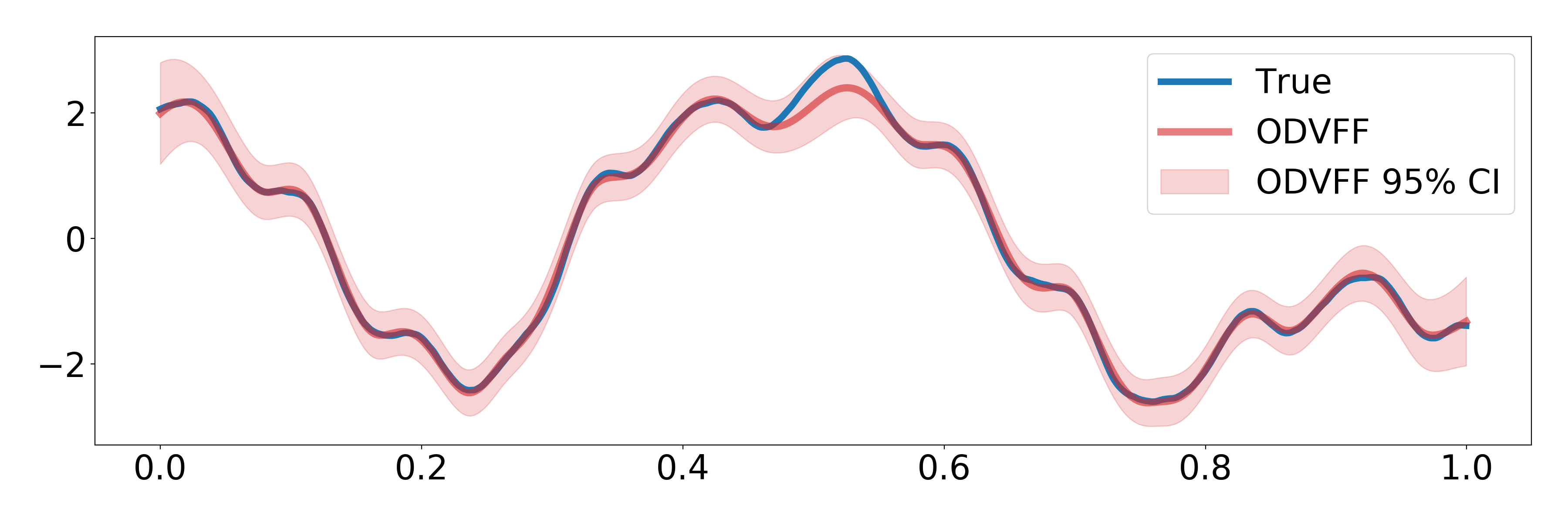
Figure 3 shows an example where data generated from a GP with an additive kernel sum of a Matern () and periodic kernel. We used a period of and lengthscales of and generated training data points from a realization of the GP. We tested on data points generated from the same realization. The ODVFF obtains a test log-likelihood of and a test RMSE of . For reference a full GP implementation obtains a test log-likelihood of and a tRMSE of .
Appendix D Further experimental results
D.1 Synthetic data
In this section we report the results for the experiments on synthetic data introduced in Section 5, main text.
| ODVFF | 0.221 | 0.214 | 0.228 | 0.210 |
|---|---|---|---|---|
| ODVGP | 0.224 | 0.214 | 0.221 | 0.212 |
| SVGP | 0.242 | 0.242 | 0.226 | 0.226 |
| SGPR | 0.212 | |||
| ODVFF | 0.954 | 0.960 | 0.950 | 0.870 |
|---|---|---|---|---|
| ODVGP | 0.945 | 0.944 | 0.946 | 0.830 |
| SVGP | 0.939 | 0.939 | 0.944 | 0.944 |
| SGPR | 0.949 | |||
| ODVFF | 1.320 | 1.324 | 1.306 | 1.309 |
|---|---|---|---|---|
| ODVGP | 1.316 | 1.317 | 1.304 | 1.305 |
| SVGP | 1.316 | 1.316 | 1.304 | 1.304 |
| SGPR | 1.316 | |||
| ODVFF | 0.700 | 0.544 | 0.471 | 0.542 |
|---|---|---|---|---|
| ODVGP | 0.685 | 0.532 | 0.412 | 0.446 |
| SVGP | 0.631 | 0.631 | 0.442 | 0.442 |
| SGPR | 0.953 | |||
| ODVFF | 1.536 | 1.537 | 1.556 | 1.554 |
|---|---|---|---|---|
| ODVGP | 1.526 | 1.527 | 1.547 | 1.548 |
| SVGP | 1.526 | 1.526 | 1.547 | 1.547 |
| SGPR | 1.526 | |||
| ODVFF | 0.653 | 0.719 | 0.708 | 0.766 |
|---|---|---|---|---|
| ODVGP | 0.629 | 0.422 | 0.618 | 0.364 |
| SVGP | 0.555 | 0.555 | 0.543 | 0.543 |
| SGPR | 0.948 | |||
D.2 Classification example
The orthogonally decoupled variational Fourier feature method was applied here only in regression tasks, however it is also possible to apply the method to classification tasks. In fact in the formulation described in Sections 4 and 3, main text, we can use any likelihood function . In this example we consider input data and an output vector where . We assume that the labels are assign as , where and are independent standard Gaussian noise. We consider a probit likelihood where is the c.d.f. of a standard Gaussian random variable. We can train our ODVFF method by learning the variational distribution as in the regression case.
As an example we consider here the banana dataset in Hensman et al., 2015 and we train ODVFF and SVGP with and . We train the models with iterations and mini-batch size . Figure 4 shows the decision boundary obtained with SVGP and with ODVFF. We notice how both decision boundaries closely resemble the full GP decision boundary. Here the ODVFF method was run with Kronecker product covariance kernel, however as and increase this method is not usable in practice. Here the alternative of using additive covariances results in very low accuracy, so it is also not practically viable. Alternative implementations such as the product of two Kronecker covariances described in Hensman et al., 2018 was not explored here. Nonetheless additional work is needed to make such methods more scalable in the input dimension.