Imputation procedures in surveys using nonparametric and machine learning methods: an empirical comparison
Abstract
Nonparametric and machine learning methods are flexible methods for obtaining accurate predictions. Nowadays, data sets with a large number of predictors and complex structures are fairly common. In the presence of item nonresponse, nonparametric and machine learning procedures may thus provide a useful alternative to traditional imputation procedures for deriving a set of imputed values used next for the estimation of study parameters defined as solution of population estimating equation. In this paper, we conduct an extensive empirical investigation that compares a number of imputation procedures in terms of bias and efficiency in a wide variety of settings, including high-dimensional data sets. The results suggest that a number of machine learning procedures perform very well in terms of bias and efficiency.
Médiamétrie.
Key words: Additive models; Bayesian additive regression trees (BART); CART; Cubist algorithm; Ensemble Methods; Nearest Neighbour; Item nonresponse; Random forest; Support vector regression (SVR); Survey data; Statistical learning; Tree boosting.
1 Introduction
In the last decade, the interest in machine learning methods has been growing in national statistical offices (NSO). These data-driven methods provide flexible tools for obtaining accurate predictions. The increasing availability of data sources (e.g., big data sources and satellite information) provides a rich pool of potential predictors that may be used to obtain predictions at different stages of a survey. These stages include the nonresponse treatment stage (e.g., propensity score weighting and imputation) and the estimation stage (e.g., model-assisted estimation and small area estimation). The imputation stage is the focus of the current paper.
Item nonresponse refers to the presence of missing values for some, but not all, survey variables. Frequent causes of item nonresponse include refusal to answer a sensitive question (e.g., income) and edit failures. The most common way of treating item nonresponse in NSOs is to replace a missing value with a single imputed value, constructed on the basis of a set of explanatory variables, available for both respondents and nonrespondents. A variety of imputation procedures are available, ranging from simple (e.g., mean, historical and ratio imputation) to more complex (e.g., nonparametric procedures); e.g., see Chen and Haziza, 2019 for an overview of imputation procedures in surveys. Every imputation procedure makes some (implicit of explicit) assumptions about the distribution of the variable requiring imputation. This set of assumptions is often referred to as an imputation model. At the imputation stage, it is therefore important to identify and include in the model all the appropriate explanatory variables that are predictive of the variable requiring imputation and determine a suitable model describing the relationship between and the set of explanatory variables
We distinguish parametric imputation procedures from nonparametric imputation procedures. In parametric imputation, the shape of the relationship between and is predetermined; e.g., linear and generalized linear regression models. However, point estimators based on parametric imputation procedures may suffer from bias if the functional form is misspecified or if the vector fails to include interactions or predictors accounting for curvature. In contrast, with nonparametric methods, the shape of the relationship between and is left unspecified. These methods have the ability to capture nonlinear trends in the data and tend to be robust to the non-inclusion of interactions or predictors accounting for curvature.
Commonly used nonparametric methods include kernel smoothing, local polynomial regression and spline-based regression models. While these methods provide some robustness against model misspecification, they tend to breakdown when the number predictors is large, a problem known as the curse of dimensionality. To mitigate this problem, one may employ additive models (Hastie and Tibshirani, 1986). However, when the dimension of is very large, these models tend to fail and machine learning methods may provide an interesting alternative. The class of machine learning methods, that includes tree-based models such as random forests and boosting methods, provide more flexible approaches able to adapt to complex non-linear and non-additive relationships between the survey variable requiring imputation and a set of predictors. These methods may also prove useful in the case of large data sets exhibiting a large number of observations on a large number of variables. Many machine learning procedures are relatively computationally efficient and can produce accurate predictions by offering the user a kind of automatic variable selection that may prove useful in a high-dimensional setting.
However, both a theoretical treatment and an empirical comparison of machine learning imputation procedures in the context of missing survey data are currently lacking. In this paper, we aim to fill the latter gap by conducting an extensive simulation study that investigates the performance of several nonparametric and machine learning procedures in terms of bias and efficiency. To that end, we generated several finite populations with relationships between and ranging from simple to complex and generated the missing values according to several nonresponse mechanisms. We also considered both a low-dimensional and high dimensional settings. The simulation setup and the models are described in Section 4. We restricted our attention to population totals (Section 4) and population quantiles (Section 5) as the target parameters. The following procedures were included in our comparisons: the score method (Little, 1986; Haziza and Beaumont, 2007), K nearest-neighbour (Chen and Shao, 2000), additive models based on B-spline regression, regression trees (Breiman et al., 1984), random forests (Breiman, 2001), tree-based boosting methods (Friedman, 2001) including XGBoost (Chen and Guestrin, 2016) and Bayesian additive regression trees (Chipman et al., 2010), the cubist algorithm (Quinlan et al., 1992; Quinlan, 1993) and support vector regression (Vapnik, 1998; Vapnik, 2000). In Section 3, we describe these models and the corresponding imputation procedures.
In recent years, machine learning procedures have received some attention in a survey sampling context. In the ideal situation of 100% response, the theoretical properties of model-assisted estimation procedures based on regression trees (McConville and Toth, 2019) and random forests (Dagdoug et al., 2020a) have been recently established. Dagdoug et al., 2020b studied the theoretical properties of point and variance estimators based on random forests in a context of imputation for item nonresponse and data integration; see also Tipton et al., 2013; De Moliner and Goga, 2018 for applications of random forests in surveys. A number of empirical investigations have been conducted to assess the performance of machine learning procedures in a context of propensity score estimation for unit nonresponse; e.g., Lohr et al., 2015, Gelein, 2017 and Kern et al., 2019.
The machine learning procedures described in Section 3 slightly differ from their traditional implementation because of the inclusion of the sampling weights in the construction of imputed values. However, it should be noted that most of the machine learning software packages for obtaining predicted values assume simple random sampling and cannot handle unequal weights. Modifying machine learning algorithms to account for unequal weights may prove challenging. When the design features (e.g., sampling weights, stratum indicators, etc.) are related to the survey variable requiring imputation, failing to incorporate them in the models may lead to biased estimators. To cope with this issue, we suggest to include all the appropriate design variables in the specification of the model. Standard machine learning software packages may then be safely used for creating a set of imputed values. In Section 4, we use Poisson sampling with inclusion probabilities proportional to a size variable to select repeated samples from the finite population. The size variable being related to the variable requiring imputation, including the -variable in the specified models led to satisfactory results.
2 Preliminaries
Consider a finite population of size . Let denote a survey variable and be the -values attached to unit We are interested in estimating (i) the finite population total of the -values, and (ii) the finite population quantile of order defined as where
denotes the finite population distribution function.
From we select a sample , of size , according to a sampling design with first-order inclusion probabilities .
A complete data estimator of is the well-known Horvitz-Thompson estimator
| (1) |
which is design-unbiased for provided that for all . A complete data estimator of the finite population quantile is given by
| (2) |
where
| (3) |
with denoting the Horvitz-Thompson estimator of the population size . Under mild regularity conditions (Wang and Opsomer, 2011), the complete data estimator is design-consistent for
In practice, the -variable may be prone to missing values. Let be a response indicator such that if is observed and otherwise. Let denote the set of respondents, of size and the set of nonrespondents, of size such that and . Available to the imputer is the data for as well as the values of the vector for
Let be the imputed value used to replace the missing value and
be the th value of the -variable after imputation. Point estimators of and after imputation, often referred to as imputed estimators, are readily obtained from the complete data estimators (1) and (2) by replacing with . This leads to
| (4) |
and
| (5) |
where
| (6) |
denotes the imputed estimator of .
Remark 2.1.
The population total the distribution function and the quantile of order may all be obtained as the solution of the following census estimating equation (Binder, 1983; Chen and Haziza, 2019):
| (7) |
where is a generic notation denoting a finite population parameter and is a function of . We assume that a solution to (7) exists and is unique. For instance, the population total can be obtained as a solution of (7) with ; the finite population distribution function can be obtained as a solution of (7) with Finally, the quantile of order can be obtained as a solution of (7) with Other finite population parameters can be obtained as a solution of (7); e.g., see Chen and Haziza, 2019. The imputed estimators and given respectively by (4)-(6) can be obtained by solving the following sample estimating equation:
where denotes an imputed estimator of
To construct the imputed values , we postulate the following imputation model :
| (8) | ||||
where is an unknown function. Often, the variance structure is assumed to have the form where is a known coefficient attached to unit and is an unknown parameter.
We assume that the data are Missing At Random (Rubin, 1976):
| (9) |
That is, we assume that the distribution of given is the same for both respondents and nonrespondents. If Condition (9) holds, the imputed values can be safely generated from which can be estimated from the observed data. In the context of imputation, the properties of point estimators are evaluated with respect to the joint distribution induced by the imputation, the sampling design and the unknown nonresponse mechanism. This framework is often referred to as the -framework (Chen and Haziza, 2019). Note that our simulation setup in Section 4 is consistent with the -framework as the simulation process involves (i) generating repeated finite populations; (ii) selecting a sample from each of population and (iii) generating a set of response indicators in each sample.
Deterministic imputation consists of replacing the missing by where is an estimator of the unknown regression function based on the responding units . However, deterministic imputation methods tend to distort the distribution of the survey variable requiring imputation, potentially leading to biased estimators of quantiles (Haziza, 2009; Chen and Haziza, 2019). To cope with this issue, one can recourse to random imputation that consists of adding an appropriate amount of random noise to the deterministic value . More specifically, let for , where of an estimator of (see Remark 2.2 below). We define the standardized residual
In the case of random imputation, the missing is replaced by
| (10) |
where is selected at random from the set of standardized residuals with probability .
Remark 2.2.
To obtain an estimator of one can postulate a model where is an unknown function. An estimator of is obtained by fitting a parametric or a nonparametric procedure with the square residuals as the response and as the set of predictors.
3 A description of imputation methods
3.1 Parametric regression imputation
Parametric regression assumes that the first moment (8) is given by
| (11) |
where is a vector of coefficients to be estimated and is a predetermined function. An estimator of is obtained by solving the following estimating equations based on the responding units:
| (12) |
where is a weight attached to element . Common choices for include and (Chen and Haziza, 2019). The imputed value under deterministic parametric regression imputation is given by
| (13) |
A special case of (13) is which corresponds to the customary linear regression model. In this case, the imputed value (13) reduces to
| (14) |
where
| (15) |
The imputed value given by (14) can be written as a weighted sum of the respondent -values:
| (16) |
where If the intercept is among the -variables, then for all A random counterpart of (13) is given by (10).
Another important special case of (13) is the logistic regression model,
which can be used for modeling binary variables. An estimator of is obtained by solving (12), which requires a numerical algorithm such as the Newton-Raphson procedure. To eliminate the possibility of an impossible imputed value, a missing value to a variable is typically imputed by where is a realization of a Bernoulli variable with parameter
Under deterministic or random parametric regression imputation, the imputed estimator is consistent for provided that the first moment of the imputation model (8) is correctly specified. However, this type of imputation may lead to biased estimators of quantiles. In contrast, the use of a random parametric regression imputation procedure tend to preserve the distribution of the variable requiring imputation, leading to valid estimators; see Chen and Haziza, 2019 for a discussion.
3.2 Imputation classes : the score method
The score method (Little, 1986; Haziza and Beaumont, 2007) consists of partitioning the sample into (say) imputation classes and imputing the missing values within each class independently from one class to another. It can be implemented as follows:
- Step 1:
For all , compute the preliminary values where is given by (15).
- Step 2:
Compute the empirical quantiles of order of the -values.
- Step 3:
Split the sample into classes, such that
with and .
It is common practice to use either mean imputation or random hot-deck imputation within classes. For mean imputation, the imputed value for missing in the th imputation class is given by
where are the same for all and for all For random hot-deck imputation, the imputed value is given by where the donor is selected at random from the set of donors belonging to the th imputation class with probability Note that random hot-deck imputation within classes can be viewed as mean imputation within classes with added residuals.
3.3 -nearest neighbours imputation
-nearest neighbour (NN) imputation is one of the simplest and widely used nonparametric imputation procedures. No explicit assumption is made about the regression function relating and . NN imputation consists of replacing the missing value of a recipient by the weighted average of the -values of its closest respondents in terms of the -variables.
Nearest-neighbour (NN) imputation corresponds to the limiting case of NN obtained with . NN is a donor imputation belonging to the class of hot-deck procedures (Chen and Shao, 2000) since a missing value is replaced by an actual respondent -value from the same file. NN imputation is especially useful for imputing categorical or discrete -variables; e.g., see Chen and Shao, 2000, Beaumont and Bocci, 2009 and Yang and Kim, 2019.
Let be the set of responding units closest to Any distance function in may be used to measure the closeness between two vectors and . In the simulation study presented in Section 4, we used the customary Euclidean distance. The NN imputed value for missing is given by
The imputed value obtained with NN can be written as a weighted sum of the respondent -values:
where for with NN imputation is a locally weighted procedure since the respondents lying not close enough to unit with respect to the -variables are assigned a weight equal to 0; i.e., The indicator function in the expression of can be replaced by a one-dimensional continuous kernel smoother whose role is to control the size of the weight through a tuning parameter the units lying farther from unit will be assigned a smaller weight than units lying close to it (Hastie et al., 2011).
The imputed estimator under NN imputation tends to be inefficient when the dimension of is large. Indeed, as increases, it becomes more difficult to find enough respondents around the point at which we aim to make a prediction. This phenomenon is known as the curse of dimensionality (Hastie et al., 2011, Chap. 1) for a more in-depth discussion ok the NN procedure. Also, it suffers from a model bias which is of order Nearest-neigbour imputation for missing survey data has been considered in Chen and Shao, 2000, Beaumont and Bocci, 2009 and Yang and Kim, 2019.
3.4 B-splines and additive model nonparametric regression
Spline regression is a flexible nonparametric method for fitting non-linear functions . It can be viewed as a simple extension of linear models. For simplicity, we start with a univariate -variable supported on the interval A spline function of order with equidistant interior knots, is a piecewise polynomial of degree between knots and smoothly connected at the knots. These spline functions span a linear space of dimension of with a basis function given by the -splines functions:
where if and equal to zero, otherwise; see (Schumaker, 1981; Dierckx, 1993). The -spline basis is appealing because the basis functions are strictly local: each function has the knots with for (Zhou et al., 1998), which means that its support consists of a small, fixed, finite number of intervals between knots. The unknown function is then approximated by a linear combination of basis functions with coefficients determined by a least squares criterion computed on the data (Goga et al., 2019). The missing value is then imputed by where
| (17) |
with denoting the vector of -spline basis functions, and minimizes
| (18) |
see Goga et al., 2019. The expression of is similar to that obtained with linear regression imputation given by (15) but unlike (15), the estimator (18) uses the -spline functions whose number can vary as a function of the number of knots and the order of the -spline functions. The degree of the piecewise polynomial does not seem to have a great impact on the model fits if a large enough number of interior knots is used (Ruppert et al., 2003). This is why quadratic or cubic splines are mostly used in practice and an adequate number of interior knots will allow to obtain flexible fits that capture local non-linear trends in the data. Knots are usually placed at the -quantiles and their number may have a great effect on the model fits: a large value of will lead to overfitting, in which case a penalization criterion may be used in (18), while a small value of may lead to underfitting. Ruppert et al., 2003 give a practical rule for choosing the number of interior knots :
The imputed value (17) with -spline regression can be also written as a weighted sum of the respondent -values similar to (16), for all with weights now given by These weights do not depend on the -values as in linear regression imputation and since for all Unlike linear regression imputation, the weights are now local due to the -spline functions ensuring more flexibility to model local nonlinear trends in the data.
We now turn to the multivariate case. For ease of presentation, we confine to the case of two predictors, and Additive models provide a simple way to model nonlinear trend in the data (Hastie and Tibshirani, 1986) and extend the standard linear model by allowing non-linear functions between the response variable and each of the explanatory variables, while maintaining additivity. In the case of two predictors, the relationship between and is expressed as a linear combination of unknown smooth functions and :
| (19) |
where the ’s are independent errors with mean equal to zero. The model (19) is restricted to be additive and does not account for the potential interactions among the predictors. Accounting for interactions between and would require the additional predictor to be included in the model, leading to
where is a low-dimensional interaction function fitted by using two-dimensional smoothers, such as local regression or two-dimensional splines. This is beyond the scope of this article. When the number of predictors is large, the number of potential interactions may be considerable, making the implementation of this procedure challenging. In such situations, random forests and boosting, discussed in sections 3.6 and 3.7, provide more flexible approaches. But, as pointed out by James et al., 2015, additive models provide a useful compromise between linear and fully nonparametric models.
The unknown functions and in (19) can be estimated by using two -spline basis and which leads to and where and are determined, as before, by a least square criterion. To ensure the identifiability of additional constraints such as are usually imposed. With these constraints, the estimators are simply obtained as a regression coefficient estimator, for and The imputed value for missing is given by
| (20) |
In practice, a backfitting algorithm is used to compute and iteratively (Hastie et al., 2011). However, when the number of explanatory variables is large, the algorithm may not converge and additive models tend to breakdown. Finally, random versions of (17) and (20) are obtained by adding random residuals as in (10).
3.5 Regression trees
Regression trees through the CART algorithm have been initially suggested by Breiman, 1984. Tree-based methods are simple to use in practice for both continuous and categorical variables and useful for interpretation. They form a class of algorithms which recursively split the -dimensional predictor space, the set of possible values for the -variables, into distinct and non-overlapping regions of . The prediction at point corresponds to the average of the respondent -values falling in the same region as unit . When the number of -variables is not too large, the splitting algorithm is quite fast, otherwise it may be time-consuming.
Following Creel and Krotki, 2006, we slightly adapt the original CART algorithm as well as the estimation procedure of . The CART algorithm recursively searches for the splitting variable and the splitting position (i.e., the coordinates on the predictor space where to split) leading to the greatest possible reduction in the residual mean of squares before and after splitting. More specifically, let be a region or node and let the number of units belonging to A split in consists of finding a pair where is the variable coordinates taking value between and and is the position of the split along the th coordinate, within the limits of Let be the set of all possible pairs in . The splitting process is performed by searching for the best split in the sense that
| (21) | |||||
| with | |||||
where is the measure of th variable for the th individual, , and the th coordinate of is the average of for those units such that . In (21), if and otherwise. From (21), the best split is the one that produces a tree with the smallest residuals sum of squares (James et al., 2015, Chap. 8); that is, we seek that minimizes
The missing is replaced by which corresponds to the weighted average of the respondent -values falling into the same region as
| (23) |
where is the region from containing the point With tree-based methods, the imputed value can also be expressed as
| (24) |
where with With regression trees and tree-based methods in general, the non-overlapping -regions obtained by means of the CART algorithm depend on the respondent data i.e., the same set of -variables with a different set of respondents will lead to different non-overlapping -regions. The resulting imputed estimator is similar to a post-stratified estimator based on adaptative post-strata.
Regression trees are simple to interpret and often exhibit a small model bias. However, they tend to overfit the data if each -region contains too few elements. To cope with this issue, regression trees may be pruned, meaning that superfluous splits (with respect to a penalized version of (21)) are removed from the tree. Pruning a regression tree tends to reduce its model variance at the expense of increasing the model bias; see Hastie et al., 2011. A random version of (24) is obtained by adding random residuals as in (10). Bagging and boosting methods may be used to improve the efficiency of tree-based procedures. This is discussed next.
3.6 Random forests
Random forest (Breiman, 2001) is an ensemble method which achieves better accuracy than tree-regression methods by creating a large number of different regression trees and combining them to produce more accurate predictions than a single model would. Random forests are especially efficient in complex settings such as small sample sizes, high-dimensional predictor space and complex relationships (Hamza and Larocque, 2005, Díaz-Uriarte and de Andrés, 2006, among others). Since the article of Breiman, 2001, random forests have been extensively used in various fields such as medicine (Fraiwan et al., 2012), time series analysis (Kane et al., 2014), agriculture (Grimm et al., 2008), to cite just a few. Recently, their theoretical properties have been established by Scornet et al., 2015.
There exist a number of random forest algorithms (see Biau and Scornet, 2016 for discussion). A widely used algorithm proceeds as follows (Dagdoug et al., 2020b):
- Step 1:
Consider bootstrap data sets obtained by selecting with replacement pairs from .
- Step 2:
- Step 3:
The imputed value for missing is obtained by averaging the predictions at the point of the regression tree predictions:
(25) where is the prediction for the unknown in (8) computed at and obtained with the th regression tree as described in Section 3.5. More specifically, from (23), the prediction corresponds to the weighted average of -values for falling in the same region containing .
A random version of (25) is obtained by adding random residuals as in (10). Although random forests are based on fully-grown trees, the accuracy of the predictions is improved by considering bootstrap of units and model aggregation, a procedure called bagging and used in statistical learning for reducing the variability. The number of regression trees should be large enough to ensure a good performance without harming the processing time; see Scornet, 2017. The second improvement brought by random forest is the random selection at each split of predictors, achieving decorrelated trees. The value of is typically chosen as (Hastie et al., 2011). In random forest algorithms, a stopping criterion is usually specified so that the algorithm stops once a certain condition (e.g., on the minimum number of units in each final nodes) is met.
3.7 Least square tree-boosting and other tree-boosting methods
As in bagging, boosting (Friedman, 2001) is a procedure that can be applied to any statistical learning methods for improving the accuracy of model predictions and is typically used with tree-based methods. While bagging involves the selection of bootstrap samples to create many different predictions, boosting is an iterative method that starts with a weak fit (or learner) and improves it at each step of the algorithm by predicting the residuals of prior models and adding them together to make the final prediction.
To understand how boosting works, consider a regression tree with non-overlapping regions expressed as
| (26) |
The parameter is obtained by minimizing
| (27) |
where denotes a loss function; e.g., the quadratic loss function. With the latter, given a region estimating the constant is usually straightforward as the average the -values belonging to However, finding the regions and solving (27) in a traditional way may prove challenging and computationally intensive as it requires optimizing over all the parameters jointly. To overcome this difficulty, one may use a greedy top-down recursive partitioning algorithm to find as described in Section 3.5. Alternatively, one may split the optimization problem (27) into many simple subproblems that can be solved rapidly. Boosting uses the latter and considers that the unknown has the following additive form:
| (28) |
where for are trees determined iteratively by using a forward stagewise procedure (Hastie et al., 2011): at each step, a new tree is added to the expansion without modifying the coefficients and parameters of trees already added. Each added tree, usually referred to as a weak-learner, has a small size and slowly improves the estimation of in areas where it does not perform well. For the quadratic loss function, after accounting for the survey weights, the algorithm becomes:
Step 1: Initialize the algorithm with a constant value:
and
Step 2: For to :
- (a)
Given the current model fit the regression tree that best predicts the residuals values and get the terminal regions
- (b)
Given the terminal regions the optimal constants are found as follows:
for
- (c)
Update where and
Step 3: Output and get the imputed value
| (29) |
A random version of (29) is obtained by adding random residuals as in (10). The number of trees should not be too large and, for better performances, Hastie et al., 2011 recommend to consider the same number of splits at each iteration. The value of reflects the level of dominant interactions between the -variables. The value (one split) produces boosted models with only main effects without interactions, whereas the value allows for two-variable interactions. Empirical studies suggest that generally leads to good results. As in ridge regression, shrinkage is used with tree boosting. In this case, Step 2. (c) of the above algorithm is replaced by a penalized version:
where the parameter called learning rate, is used to penalized large trees; usually or Both and control the performance of the model prediction.
3.7.1 XGBoost
Chen and Guestrin, 2016 suggested a scalable end-to-end tree boosting system called XGBoost which is extremely fast. Here, we adapt the algorithm in order to account for the survey weights. Consider again a tree with formal expression given in (26). This tree learning algorithm consists of minimizing the following objective function at the -th iteration:
| (30) |
where the penalty function penalizes large trees in order to avoid overfitting. The search problem is optimized by using a second-order Taylor approximation of and ignoring the constant term, the new optimization problem reduces to:
| (31) |
where and are the first and second-order derivatives of the loss function computed at . With the quadratic loss function, and The new objective function from (31) is a second-order polynomial with respect to , so the optimal is easily obtained as leading to the optimal value of the objective function as This value is then used next as a decision criterion in a greedy top-down recursive algorithm to find the optimal regions of the -th tree to be added.
3.7.2 Bayesian additive regression trees (BART)
Bayesian additive regression trees (Chipman et al., 2010, BART) is similar to boosting in the sense that the unknown regression function has an additive form as in (28). While boosting is completely nonparametric, BART makes a Gaussian assumption on the model errors:
where is assumed to be a sum of tree functions and is the set of parameter values associated with the terminal nodes in each tree .
As stated in Chipman et al., 2010, although similar in spirit to gradient boosting, BART differs from boosting algorithms both by the way it weakens the individual trees by relying on a Bayesian framework, but also on how it performs the iterative fitting. More specifically, a prior is specified for the parameters of the model and . The prior of can be decomposed into three components :
- 1.
The probability that a node at depth is a terminal node is given by for
- 2.
The distribution on the splitting variable assignments in each interior node is uniform.
- 3.
The distribution of the splitting value conditional on the chosen splitting variable is also uniform.
Borrowing the illustrative example of Chipman et al., 2010, with the parameters and , trees with terminal nodes receive prior probabilities of and , respectively. Therefore, as in boosting, the BART model tends to favor trees with a small number of terminal nodes. However, the process of restricting the depth of regression trees (or equivalently the number of terminal nodes) in BART is different from the one used in boosting. For boosting, the depth of the trees is fixed by the user and is similar for all trees used in the forest. For BART, the user specifies a probability for the trees to have a certain number of terminal nodes. As a result, the number of terminal nodes is random rather tan fixed. Therefore, it is likely that trees have only a small number of terminal nodes with the BART model, but this number can vary depending on the data at hand. For , a conjugate prior is chosen to make computations simpler; e.g., is assumed to be . Similarly, a conjugate prior is chosen for , e.g., the inverse chi-square distribution. To generate the posterior distribution, the authors suggest the use of a Gibbs sampler. For general guidelines about the choices of these parameters, see Chipman et al., 2010. The imputed value for missing is obtained as with the general boosting algorithm given in Section 3.7, where the prediction of each regression tree is the weighted average of the values in the terminal node containing .
3.8 Cubist algorithm
Cubist is an updated implementation of the M5 algorithm introduced by Quinlan et al., 1992 and Quinlan, 1993. It is an algorithm based on regression trees and linear models, among other ingredients. Initially, Cubist was only available under a commercial license. In 2011, the code was released as open-source. The algorithm proceeds as follows (Kuhn and Johnson, 2013, Chap. 8):
- Step 1:
Create a partition of To do so, let be the set of all possible splits in a node of cardinality , that is, the set of all possible pairs (position, variable). Then, the split is performed using the following criterion:
where denote the non-terminal nodes after each of the previous splits and denotes the cardinal of elements in the node .
- Step 2:
In each node, a linear model is fitted between the survey variable and the auxiliary variables that have been used to split the tree. More specifically, consider the th terminal node . Then, there exists a path from the first node to the current node in the graph formed by the tree. This path uses variables among the set . For instance, assume that a partition of elements is created by the tree shown in Figure 1. Then, the linear model in the node is fitted using the variables that created the path in red, that is, , and , and so for this node. The linear model fitted in the node uses only one variable, (the green path), so .
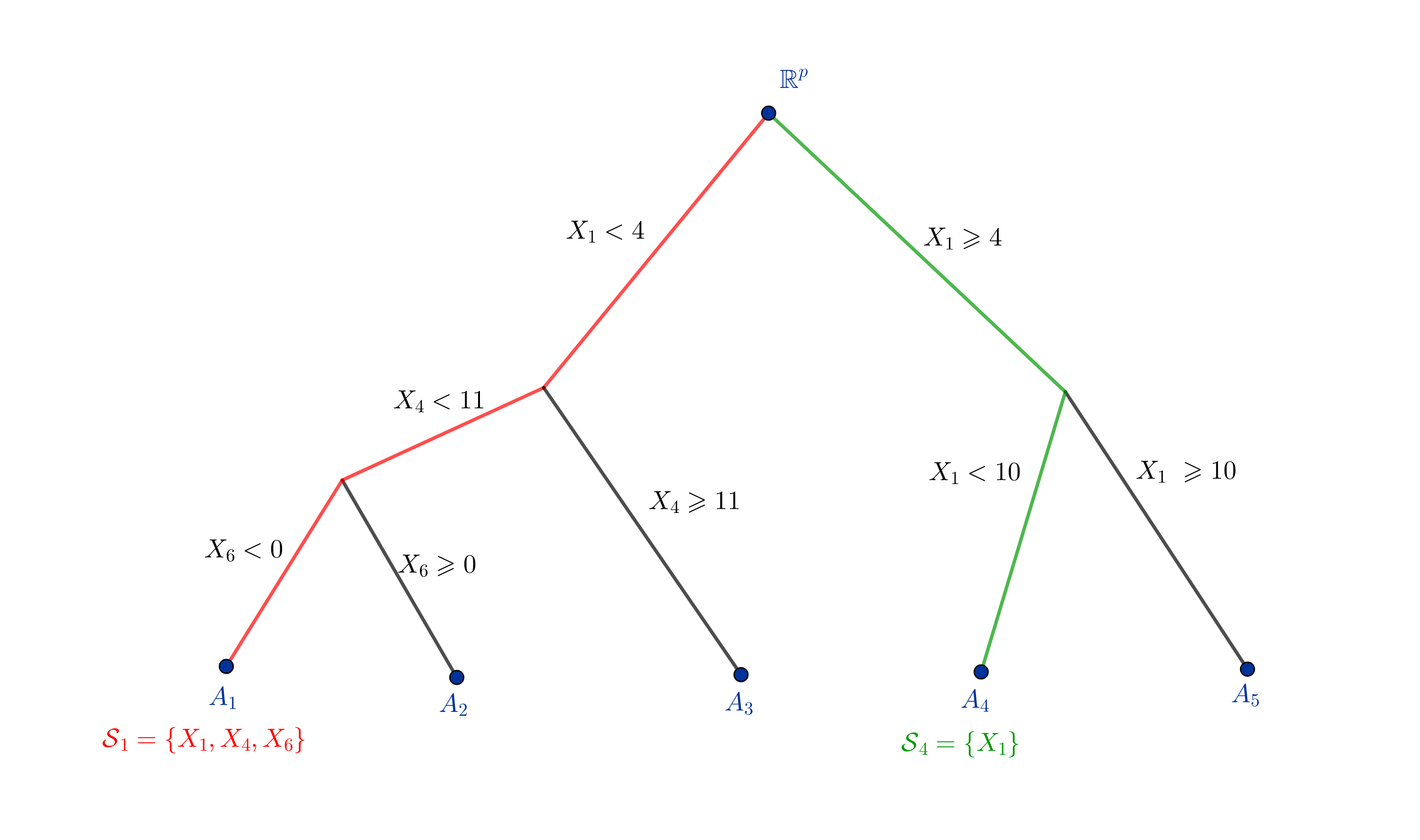
Figure 1: Example of a graph induced by a tree algorithm. The coefficients of the linear model in the node are estimated using the customary weighted least squares criterion:
where is the vector containing the measurements of the variables for unit .
- Step 3:
In each node, a backward elimination procedure is performed using the adjusted error rate (AER) criterion. For instance, in the th terminal node, we have
where denotes the number of variables used in the current model which predicts for a prediction at the point . Each variable in the initial model is dropped and the AER is recomputed. Terms are dropped from the model as long as the AER decreases.
- Step 4:
Once the tree is fully grown, it is pruned by removing unnecessary splits. Starting at the terminal nodes, the AER is computed with and without the node. Whenever the node does not result in a decrease of the AER, it is pruned. This process is performed until no more node can be removed.
- Step 5:
To avoid over-fitting, a smoothing procedure is performed. Let be the predicted value obtained by fitting the linear model in the th child node and be the predicted value obtained from the direct parent node. These predictions are combined as
where
with denoting the th coordinate of the vector , denoting the th coordinate of the vector and and denoting the empirical model variance and covariance, respectively.
- Step 6:
Cubist can be used as an ensemble model. Once the Cubist algorithm is fitted, the subsequent iterations of the algorithm use the previously trained algorithm to define an adjusted response so that the next iteration of the algorithm uses
where is the value of the adjusted response for the th iteration of the Cubist algorithm.
- Step 7:
The final imputed value for missing is derived using a nearest-neighbour rule:
(32) where denotes the distance between and the th neighbor, denotes the outcome of the th neighbor and its predicted value.
A random version version of (32) is obtained by adding random residuals as in (10).
3.9 Support vector regression
Support vector machines (Vapnik, 1998; Vapnik, 2000; Cortes and Vapnik, 1995; Smola and Schölkopf, 2004) belong to the class of supervised learning algorithms and may be used for regression analysis. We start by considering the linear regression model
before discussing the case of nonlinear relationships. In the customary regression framework, the goal is to minimize the residuals sum of squares. In Support Vector Regression (SVR), the goal is to minimize a function of the residuals plus a -penalization on the regression coefficient:
| (33) |
where is the so-called -insensitive error measure defined as if and otherwise (Vapnik, 2000) for can be viewed as the allowed tolerance for fitting; see Figure 1 in Smola and Schölkopf, 2004. The optimization problem (33) may not have solution and supplementary tolerances (called also "the slack variables") on the individual fitted errors are considered (Smola and Schölkopf, 2004). There exist several ways for incorporating weights in the optimization problem, leading to different weighted support vector regression solutions. We consider the method suggested by Lee et al., 2005 and Han and Clemmensen, 2014:
| (34) |
and
| (35) | ||||||
where is the tuning parameter that provides a trade-off between the smoothness of the fitted function and the deviation from the training data and denotes the normalized sampling weight associated with unit . As a result, the ’s are all smaller than one. As argued by Han and Clemmensen, 2014, incorporating weights in the objective function as in (34) has the effect of shrinking the estimators to different extents. The solution of (33) and (35) is given by which leads to
| (36) |
where is an inner product and and denote the Lagrange multipliers verifying the quadratic programming problem:
subject to and As a result, only a subset of the solution values are nonzero and the associated data values are called the support vectors. The solution is written as a linear combination of these support vectors. Moreover, the prediction uses only the support vectors and the inner products between and without requiring the computation of This property is useful for extending the method to handle nonlinear relationships.
We now consider the case of a nonlinear and unknown function We approximate in a basis of functions as follows:
and and minimize (34) and
| (37) | ||||||
A similar derivation as before leads to for and
where is a positive definite kernel (Smola and Schölkopf, 2004). The computation of involves only through inner products and using a kernel function makes the computation of possible without requiring All is needed is the knowledge of . Using , it is possible to solve the optimization problem in a higher-dimensional space without having to compute any product in this space. Common choices of include the Gaussian kernel and the polynomial kernel The imputed value for the missing is given by
| (38) |
A random version version of (38) is obtained by adding random residuals as in (10). The reader is referred to Smola and Schölkopf, 2004 for a discussion on how to estimate
4 Simulation study: the case of population totals
We conducted an extensive simulation study to investigate the performance of the imputation procedures described in Section 3 in terms of bias and efficiency.
4.1 The setup
For each scenario, we repeated iterations of the following process:
- (i)
A finite population of size was generated. The population consisted of a survey variable and a set of predictors .
- (ii)
From the finite population generated in Step (i), a sample, of size was selected according to a given probability sampling design.
- (iii)
In each sample, nonresponse to item was generated according to a given nonresponse mechanism.
- (iv)
The missing values in each sample were imputed using several imputation procedures.
We now give a more in-depth discussion of each of the steps (i)-(iv).
We first generated five predictors according to the following distributions: followed a normal distribution, followed a Beta distribution, followed a Gamma distribution, followed a Bernoulli distribution, and followed a multinomial distribution, The predictors - were continuous, whereas the predictors and were discrete. The predictors - were standardized so as to have a zero mean and a variance equal to one. Given the predictors - we generated the continuous survey variables according to the following models:
- •
;
- •
;
- •
;
- •
;
- •
;
- •
;
- •
;
- •
;
and the binary survey variables as follows:
- •
where
- •
where
with
(39)
For the survey variables and , note that we have generated errors for non-normal distribution to assess the robustness of the BART procedure that assumes a Gaussian distribution for the errors.
From each population, we selected samples, of (expected) size according to two sampling designs: (a) simple random sampling without replacement and (b) Poisson sampling with probability proportional to the values of the variable ; i.e., for all Simple random sampling without replacement was used for estimating the finite population total of the continuous survey variables - and and the binary variables and whereas Poisson sampling was used for estimating the totals of the survey variables and
In each sample, nonresponse to the survey variable was generated according to four nonresponse mechanisms. That is, the response indicators were generated from a Bernoulli distribution with probability where
where is the th value of given by (• ‣ 4.1). In (NR1)-(NR4), the model parameters were set so as to obtain a response rate of about in each sample.
In each sample, the missing values were imputed according to eleven imputation procedures described in section 3. Some of the imputation procedures required the specification of some parameters (e.g., regularization parameter, depth of a regression tree, choice of a kernel, etc.). We have included several configurations to assess the impact of these parameters on the performance of these procedures. Based on the different configurations, we ended up with twenty-seven imputation procedures. More specifically, we included the following procedures:
- Procedure 1:
"LR" : Deterministic linear regression imputation; see Section 3.1.
- Procedure 2:
"MWC" : Mean imputation within classes, where the number of units in each class was set to see Section 3.2.
- Procedure 3:
"HDWC" : Random hot-deck imputation within classes, where the number of units in each class was set to ; see Section 3.2.
- Procedure 4:
"NN" : -Nearest-Neighbours imputation with and nearest neighbours and the euclidian distance and implemented with the -package caret; see Section 3.3.
- Procedure 5:
"AMS" : Additive models based on cubic -splines with equidistant interiors knots placed at the -quantiles, where and implemented with the -package mgcv; see Section 3.4.
- Procedure 6:
"CART" : Imputation through regression trees with the CART algorithm and implemented with the -package rpart; see Section 3.5.
- Procedure 7:
"RF1" : Imputation through random forest with trees, one observation per terminal node and 1 predictor considered for the search in each split. "RF2": Random forest with trees, 5 observations per terminal node and predictors considered for each split, where is the number of -variables used in the imputation model, in our case . "RF3" : Random forest with trees, 10 observations per terminal node and predictors considered for each split. Simulations were implemented with the -package ranger; see Section 3.6.
- Procedure 8:
"XGB1": XGBoost algorithm with trees each one with final splits and a learning rate of . "XGB2": XGBoost algorithm with trees with and a learning rate of . "XGB3": XGBoost algorithm with trees with and a learning rate of . Simulations were implemented with the -package xgboost; see Section 3.7.1.
- Procedure 9:
"BART" : Imputation through Bayesian additive regression trees. Simulations were implemented with the -package bartMachine; see Section 3.7.2.
- Procedure 10:
"CUBIST1": Cubist with one model. "CUBIST2" : Cubist with five models. "CUBIST3" : Cubist with 5 models and unbiased estimation. Simulations were implemented with the -package Cubist; see Section 3.8.
- Procedure 11:
"SVR1": Support vector regression imputation with a Gaussian kernel and the objective function. "SVR2": Support vector regression imputation with a polynomial kernel of degree 3 and the -insensitive objective function. "SVR3": Support vector regression imputation with a Gaussian kernel and the -insensitive objective function. "SVR4": Support vector regression imputation with a linear kernel and the -insensitive objective function. Simulations were implemented with the -package e1071; see Section 3.9.
The imputation procedures used in our simulations were based on an imputation model that included the predictors without any interaction terms. Except for random hot-deck imputation (Procedure 3) and nearest-neighbour imputation (Procedure 4 with ), for the binary variables and , note that we have generated zeroes and ones from independent Bernoulli distributions with parameter where denotes the predicted value associated with unit . Whenever , we set it to . Similarly, when we set it to .
As a measure of bias of the imputed estimator given by (4), we computed the Monte Carlo percent relative bias defined as
| (40) |
where denotes the imputed estimator at the th iteration, .
As a measure of efficiency, we computed the relative of efficiency, using the complete data estimator given by (1), as the reference. That is,
| (41) |
where and is defined similarly.
4.2 Simulation results
In Section 4.2.1, we discuss the simulation results pertaining to the continuous survey variables and with simple random sampling without replacement. The results for Poisson sampling used in the case of and are discussed in Section 4.2.2. Finally, the case of the binary variables and whose totals were estimated with simple random sampling without replacement, is discussed in Section 4.2.3.
4.2.1 Continuous survey variables and simple random sampling without replacement
For simple random sampling without replacement, for each of the twenty-seven imputation procedures, we had seven survey variables and four nonresponse mechanisms, leading to sets of simulation results. For ease of presentation, we present the results in tabular and graphic forms. The displayed statistical analyses were obtained from scenarios obtained by crossing all the nonresponse models and the survey variables.
For each imputation procedure, Table 1 and Table 2 display, respectively, some descriptive statistics regarding the Monte Carlo absolute percent relative bias (absolute value of RB) and the Monte Carlo relative efficiency (RE) of calculated across the twenty-eight scenarios. The corresponding side-by-side boxplots obtained from the twenty-eight scenarios are given in Figures 2 and 3. In Tables 1 and 2, the imputation procedures are ordered from the best to the worst with respect to the median absolute percent RB (the median of the twenty-eight values of absolute RB) and the median percent RE (the median of the twenty-eight values of RE), respectively. Figure 4 shows the distribution of the imputed estimator for the best ten imputation procedures in terms of RE. Finally, Table 3 displays the best five imputation procedures for each -variable.
From Table 1 and Table 2, among the twenty-seven imputation procedures, the best methods were: CUBIST, XGboost, AMS and BART. The performance of CUBIST3 was especially impressive with a median RE of 115%, a value of equal to 158% and a maximum value of 211%. The methods XGboost, AMS and BART exhibited similar performances with values of median RE ranging from 122% and 129%. However, for some scenarios, these methods did not perform well. For instance, the procedure XGB2 showed a value of max RE of about 438%, whereas it was equal to 1728% for AM5. Results suggest that additive models with 5 interiors knots perform better than those with 10 interior knots. The next group of imputation procedures includes SVR and RF, with values of median RE ranging from 141% and 151%. Again, for some scenarios, both methods displayed poor performances with values of max RE ranging from 322% to 1138%. The procedure CART was less efficient than RF2 and RF3. The procedure -NN did relatively well with a median RE equal to 194%. On the other hand, the procedure -NN was rather inefficient with a median RE of 229%, which suggests that NN with survey data works well only with a small number of neighbour. Turning to mean and random hot-deck imputation within classes, the score method was outperformed by the aforementioned procedures. Among the different versions of MCW and HDWC, the procedure MWC50 (which corresponds to 20 classes) led to the best results. This is consistent with the results of Haziza and Beaumont, 2007. As expected, the procedure HDWC50 was less efficient than MWC50 as random hot-deck imputation suffers from the imputation variance, arising from the random selection of donors within classes. Finally, for some scenarios, it is worth noting that some of the procedures were better than the complete data estimator. For instance, for SVR4, the minimum value of RE and the value of were respectively equal to 82% and 89%, respectively (see Table 2). Finally, the results in Table 5 suggest that the best methods were CUBIST, XGBoost, additive models and BART, which is consistent with the discussion above.
For each of the best ten imputation procedures displayed Table 2, Figure 5 displays the distribution of for each nonresponse mechanism. Figure 5 suggests that the nonresponse mechanism may have a considerable impact on the behavior of the imputed estimator. For instance, in our experiments, we note that most of the imputation procedures performed poorly in the case of the nonresponse mechanism (NR1). Notable exceptions were AMS5, BART and Cubist3. In particular, Cubist3 seemed to be insensitive to the nonresponse mechanism, which is a desirable feature.
| Ranking | Model | Min | Max | |||||||||||||
|---|---|---|---|---|---|---|---|---|---|---|---|---|---|---|---|---|
| 1 | CUBIST3 | 0.0 | 0.0 | 0.0 | 0.1 | 0.9 | 2.8 | 3.5 | ||||||||
| 2 | AMS5 | 0.0 | 0.0 | 0.0 | 0.1 | 1.8 | 7.7 | 13.8 | ||||||||
| 3 | AMS10 | 0.0 | 0.0 | 0.0 | 0.1 | 1.8 | 7.6 | 13.5 | ||||||||
| 4 | CUBIST1 | 0.0 | 0.0 | 0.1 | 0.5 | 3.4 | 7.5 | 7.5 | ||||||||
| 5 | XGB1 | 0.0 | 0.0 | 0.2 | 0.6 | 1.8 | 4.2 | 5.4 | ||||||||
| 6 | MWC50 | 0.0 | 0.0 | 0.1 | 0.6 | 2.7 | 8.3 | 11.7 | ||||||||
| 7 | HDWC50 | 0.0 | 0.0 | 0.1 | 0.6 | 2.7 | 8.3 | 11.8 | ||||||||
| 8 | CUBIST2 | 0.0 | 0.0 | 0.1 | 0.6 | 3.6 | 7.5 | 7.5 | ||||||||
| 9 | BART | 0.0 | 0.1 | 0.4 | 0.8 | 2.2 | 4.0 | 4.6 | ||||||||
| 10 | XGB2 | 0.1 | 0.2 | 0.4 | 0.9 | 2.8 | 5.4 | 10.1 | ||||||||
| 11 | LR | 0.0 | 0.0 | 0.1 | 0.9 | 3.8 | 12.8 | 20.4 | ||||||||
| 12 | SVR3 | 0.1 | 0.1 | 0.4 | 1.0 | 3.2 | 7.1 | 13.5 | ||||||||
| 13 | MWC100 | 0.0 | 0.0 | 0.3 | 1.0 | 3.6 | 10.1 | 12.9 | ||||||||
| 14 | HDWC100 | 0.0 | 0.0 | 0.3 | 1.0 | 3.6 | 10.1 | 12.9 | ||||||||
| 15 | SVR1 | 0.0 | 0.1 | 0.4 | 1.2 | 3.4 | 7.4 | 14.0 | ||||||||
| 16 | RF3 | 0.0 | 0.2 | 0.5 | 1.3 | 3.8 | 16.6 | 20.7 | ||||||||
| 17 | RF2 | 0.0 | 0.1 | 0.4 | 1.4 | 4 | 15.6 | 18.6 | ||||||||
| 18 | MWC250 | 0.0 | 0.0 | 0.7 | 1.7 | 4.9 | 14.6 | 18.1 | ||||||||
| 19 | HDWC250 | 0.0 | 0.0 | 0.6 | 1.7 | 4.9 | 14.6 | 18.1 | ||||||||
| 20 | RF1 | 0.1 | 0.2 | 0.9 | 1.7 | 7.7 | 32.1 | 39.5 | ||||||||
| 21 | NN | 0.0 | 0.1 | 1.0 | 2.1 | 5.2 | 8.0 | 9.4 | ||||||||
| 22 | MWC500 | 0.0 | 0.0 | 0.7 | 2.2 | 7.2 | 25.5 | 30.6 | ||||||||
| 23 | CART | 0.0 | 0.1 | 0.1 | 2.4 | 4.9 | 17.4 | 28.0 | ||||||||
| 24 | X5NN | 0.0 | 0.2 | 1.5 | 3 | 7.3 | 12.0 | 13.7 | ||||||||
| 25 | SVR2 | 0.1 | 0.2 | 1.0 | 3.7 | 11.7 | 19.9 | 27.0 | ||||||||
| 26 | XGB3 | 0.6 | 1.5 | 3.1 | 4.3 | 5.0 | 9.5 | 10.3 | ||||||||
| 27 | SVR4 | 0.0 | 0.0 | 2.4 | 5.3 | 7.8 | 22.2 | 33.3 |
| Ranking | Model | Min | Max | |||||||||||||
|---|---|---|---|---|---|---|---|---|---|---|---|---|---|---|---|---|
| 1 | CUBIST3 | 102 | 102 | 111 | 115 | 125 | 158 | 211 | ||||||||
| 2 | BART | 113 | 113 | 116 | 122 | 131 | 154 | 204 | ||||||||
| 3 | AMS5 | 100 | 101 | 111 | 123 | 147 | 378 | 1728 | ||||||||
| 4 | AMS10 | 100 | 101 | 112 | 123 | 167 | 1195 | 1749 | ||||||||
| 5 | XGB1 | 101 | 103 | 115 | 129 | 153 | 203 | 288 | ||||||||
| 6 | CUBIST2 | 102 | 103 | 119 | 133 | 187 | 360 | 365 | ||||||||
| 7 | XGB2 | 102 | 102 | 117 | 133 | 166 | 316 | 438 | ||||||||
| 8 | CUBIST1 | 103 | 105 | 120 | 136 | 182 | 360 | 365 | ||||||||
| 9 | SVR1 | 94 | 103 | 122 | 141 | 180 | 284 | 322 | ||||||||
| 10 | SVR3 | 95 | 106 | 122 | 143 | 181 | 269 | 299 | ||||||||
| 11 | RF3 | 115 | 118 | 131 | 149 | 192 | 919 | 1138 | ||||||||
| 12 | RF2 | 113 | 118 | 130 | 151 | 202 | 824 | 1025 | ||||||||
| 13 | CART | 125 | 134 | 143 | 168 | 248 | 1498 | 2683 | ||||||||
| 14 | LR | 110 | 111 | 114 | 169 | 315 | 823 | 3494 | ||||||||
| 15 | MWC50 | 113 | 114 | 122 | 171 | 205 | 308 | 583 | ||||||||
| 16 | HDWC50 | 120 | 120 | 128 | 189 | 240 | 332 | 600 | ||||||||
| 17 | MWC100 | 116 | 116 | 136 | 191 | 217 | 296 | 670 | ||||||||
| 18 | NN | 101 | 111 | 125 | 194 | 378 | 486 | 526 | ||||||||
| 19 | XGB3 | 92 | 100 | 128 | 194 | 663 | 1082 | 1104 | ||||||||
| 20 | HDWC100 | 123 | 125 | 142 | 213 | 246 | 322 | 686 | ||||||||
| 21 | RF1 | 136 | 137 | 149 | 223 | 375 | 3656 | 3916 | ||||||||
| 22 | MWC250 | 128 | 130 | 159 | 229 | 279 | 383 | 1162 | ||||||||
| 23 | 5NN | 94 | 108 | 123 | 229 | 659 | 775 | 855 | ||||||||
| 24 | SVR2 | 97 | 102 | 151 | 242 | 1616 | 3849 | 6355 | ||||||||
| 25 | SVR4 | 82 | 89 | 117 | 258 | 1439 | 4301 | 8675 | ||||||||
| 26 | HDWC250 | 141 | 143 | 185 | 265 | 325 | 411 | 1184 | ||||||||
| 27 | MWC500 | 151 | 155 | 202 | 269 | 336 | 1783 | 3021 |


| Ranking | Y1 | Y2 | Y3 | Y4 | Y5 | Y6 | Y7 | Y8 | ||||||||
|---|---|---|---|---|---|---|---|---|---|---|---|---|---|---|---|---|
| 1 | LR | CUBIST3 | AMS5 | BART | XGB3 | CUBIST3 | CUBIST3 | CUBIST3 | ||||||||
| 2 | CUBIST3 | LR | AMS10 | CUBIST3 | AMS5 | BART | AMS5 | AMS5 | ||||||||
| 3 | MW50 | AMS5 | BART | CUBIST1 | AMS10 | SVR3 | AMS10 | AMS10 | ||||||||
| 4 | AMS5 | MWC50 | CUBIST3 | CUBIST2 | XGB1 | SVR1 | MWC50 | XGB1 | ||||||||
| 5 | AMS10 | AMS10 | CUBIST2 | XGB1 | XGB2 | XGB1 | BART | BART |
4.2.2 Continuous survey variables with Poisson sampling
Recall that Poisson sampling was used for estimating the population total of the survey variables and . This led to sets of results. Due to the small number of scenarios () for each of the survey variables and , Tables 4 and 5 show the minimum, the median and the maximum Monte Carlo percent absolute RB and Monte Carlo percent RE only. The size variable used to obtain the first-order inclusion probabilities was included as a predictor in the imputation models. The results in Tables 4 and 5 were consistent with those obtained for simple random sampling without replacement. Again, the best methods were CUBIST3, BART and XGB1 in terms of either bias or efficiency.
| Ranking | Model | Min | Max | |||||
|---|---|---|---|---|---|---|---|---|
| 1 | BART | 0.1 | 0.9 | 3.0 | ||||
| 2 | CUBIST3 | 0.0 | 1 | 6.5 | ||||
| 3 | XGB1 | 0.0 | 2.4 | 5.2 | ||||
| 4 | CUBIST1 | 0.0 | 3.4 | 10.9 | ||||
| 5 | RF2 | 0.3 | 3.5 | 15.8 | ||||
| 6 | RF3 | 0.5 | 3.5 | 16.8 | ||||
| 7 | XGB2 | 0.4 | 3.9 | 8.6 | ||||
| 8 | AMS5 | 0.2 | 4.3 | 11.1 | ||||
| 9 | AMS10 | 0.2 | 4.3 | 10.7 | ||||
| 10 | CUBIST2 | 0.0 | 4.3 | 12.6 | ||||
| 11 | RF1 | 0.8 | 4.4 | 31.4 | ||||
| 12 | SVR3 | 0.1 | 4.4 | 6.7 | ||||
| 13 | LR | 0.2 | 4.9 | 16.8 | ||||
| 14 | SVR1 | 0.1 | 4.9 | 7.1 | ||||
| 15 | MWC500 | 0.0 | 5.0 | 26.1 | ||||
| 16 | NN | 0.0 | 5.0 | 7.3 | ||||
| 17 | MWC250 | 0.0 | 5.1 | 14.7 | ||||
| 18 | HDWC50 | 0.8 | 5.1 | 9.9 | ||||
| 19 | MWC50 | 0.0 | 5.2 | 9.9 | ||||
| 20 | MWC100 | 0.0 | 5.2 | 10.1 | ||||
| 21 | HDWC100 | 0.1 | 5.2 | 10.0 | ||||
| 22 | HDWC250 | 0.0 | 5.2 | 14.7 | ||||
| 23 | CART | 0.2 | 5.6 | 24.6 | ||||
| 24 | 5NN | 1.3 | 7.1 | 11.7 | ||||
| 25 | XGB3 | 2.5 | 8.8 | 11.1 | ||||
| 26 | SVR2 | 1.0 | 11.7 | 22.6 | ||||
| 27 | SVR4 | 0.2 | 15.4 | 27.5 |
| Ranking | Model | Min | Max | |||||
|---|---|---|---|---|---|---|---|---|
| 1 | BART | 106 | 117 | 139 | ||||
| 2 | CUBIST3 | 111 | 118 | 239 | ||||
| 3 | XGB1 | 108 | 133 | 207 | ||||
| 4 | RF2 | 114 | 144 | 565 | ||||
| 5 | RF3 | 114 | 145 | 621 | ||||
| 6 | XGB2 | 110 | 156 | 246 | ||||
| 7 | SVR3 | 109 | 165 | 198 | ||||
| 8 | AMS5 | 124 | 168 | 486 | ||||
| 9 | SVR1 | 109 | 175 | 209 | ||||
| 10 | CUBIST1 | 114 | 175 | 469 | ||||
| 11 | NN | 117 | 178 | 234 | ||||
| 12 | MWC50 | 125 | 188 | 396 | ||||
| 13 | MWC100 | 125 | 188 | 363 | ||||
| 14 | RF1 | 122 | 188 | 1868 | ||||
| 15 | LR | 123 | 189 | 923 | ||||
| 16 | MWC250 | 128 | 190 | 525 | ||||
| 17 | CUBIST2 | 111 | 193 | 548 | ||||
| 18 | CART | 133 | 198 | 1224 | ||||
| 19 | MWC500 | 133 | 198 | 1346 | ||||
| 20 | HDWC50 | 135 | 210 | 409 | ||||
| 21 | HDWC100 | 139 | 213 | 381 | ||||
| 22 | HDWC250 | 145 | 217 | 539 | ||||
| 23 | 5NN | 120 | 241 | 370 | ||||
| 24 | XGB3 | 116 | 272 | 441 | ||||
| 25 | AMS10 | 130 | 313 | 592 | ||||
| 26 | SVR2 | 142 | 493 | 1619 | ||||
| 27 | SVR4 | 141 | 769 | 2119 |
4.2.3 Binary survey variables
In this section, we present the results pertaining to the binary variables and . Again, for each imputation procedure, we obtained sets of results. Tables 6 and 7 show the minimum, the median and the maximum Monte Carlo percent absolute RB and Monte Carlo percent RE, respectively.
The ranking for binary survey variables was slightly different from that obtained for the continuous survey variables. Nearest-neighbor (NN) imputation procedure was the best in terms of bias and efficiency. Recall that NN imputation did not rank among the best procedures for the continuous variables. NN imputation was followed by CUBIST, XGBOOST and BART.
| Ranking | Model | Min | Max | |||||
|---|---|---|---|---|---|---|---|---|
| 1 | NN | 136 | 144 | 428 | ||||
| 2 | XGB3 | 153 | 165 | 860 | ||||
| 3 | XGB2 | 156 | 167 | 827 | ||||
| 4 | CUBIST3 | 156 | 167 | 841 | ||||
| 5 | XGB1 | 156 | 171 | 932 | ||||
| 6 | BART | 156 | 173 | 1052 | ||||
| 7 | 5NN | 152 | 174 | 1191 | ||||
| 8 | CUBIST2 | 163 | 179 | 873 | ||||
| 9 | CUBIST1 | 169 | 191 | 904 | ||||
| 10 | RF2 | 158 | 192 | 1572 | ||||
| 11 | RF3 | 162 | 198 | 1769 | ||||
| 12 | AMS5 | 169 | 219 | 2453 | ||||
| 13 | MWC100 | 160 | 221 | 1120 | ||||
| 14 | MWC50 | 159 | 222 | 1067 | ||||
| 15 | SVR1 | 171 | 222 | 3196 | ||||
| 16 | AMS10 | 165 | 223 | 2472 | ||||
| 17 | MWC50 | 159 | 223 | 1061 | ||||
| 8 | M100 | 159 | 225 | 1116 | ||||
| 19 | CART | 176 | 229 | 1882 | ||||
| 20 | LR | 164 | 230 | 2707 | ||||
| 21 | MWC250 | 172 | 244 | 1460 | ||||
| 22 | MWC250 | 173 | 246 | 1471 | ||||
| 23 | SVR3 | 191 | 280 | 2899 | ||||
| 24 | RF1 | 190 | 305 | 4666 | ||||
| 25 | M500 | 186 | 365 | 4977 | ||||
| 26 | SVR4 | 219 | 409 | 26429 | ||||
| 27 | SVR2 | 413 | 1839 | 17279 |
| Ranking | Model | Min | Max | |||||
|---|---|---|---|---|---|---|---|---|
| 1 | NN | 0.0 | 0.5 | 3.6 | ||||
| 2 | CUBIST3 | 0.02 | 0.7 | 6.7 | ||||
| 3 | XGB3 | 0.03 | 0.8 | 7.7 | ||||
| 4 | BART | 0.1 | 0.8 | 8.8 | ||||
| 5 | XGB1 | 0.14 | 0.9 | 7.9 | ||||
| 6 | XGB2 | 0.0 | 0.9 | 6.9 | ||||
| 7 | 5NN | 0.0 | 1.0 | 7.3 | ||||
| 8 | CUBIST2 | 0.2 | 1.0 | 7.0 | ||||
| 9 | CUBIST1 | 0.0 | 1.1 | 6.8 | ||||
| 10 | RF2 | 0.12 | 1.5 | 10.3 | ||||
| 11 | RF3 | 0.13 | 1.6 | 11.0 | ||||
| 12 | AMS5 | 0.04 | 1.6 | 11.9 | ||||
| 13 | AMS10 | 0.1 | 1.6 | 11.9 | ||||
| 14 | SVR1 | 0.3 | 1.7 | 12.0 | ||||
| 15 | LR | 0.19 | 1.8 | 12.3 | ||||
| 16 | CART | 0.18 | 1.8 | 11.4 | ||||
| 17 | MWC50 | 0.0 | 1.8 | 7.5 | ||||
| 18 | MWC100 | 0.0 | 1.8 | 7.7 | ||||
| 19 | HDWC50 | 0.03 | 1.8 | 7.5 | ||||
| 20 | HDWC100 | 0.01 | 1.8 | 7.7 | ||||
| 21 | MWC250 | 0.0 | 2.0 | 9.4 | ||||
| 22 | HDWC250 | 0.0 | 2.0 | 9.4 | ||||
| 23 | SVR3 | 0.43 | 2.3 | 11.5 | ||||
| 24 | RF1 | 0.08 | 2.7 | 19.0 | ||||
| 25 | SVR4 | 0.17 | 3.0 | 36.5 | ||||
| 26 | MWC500 | 0.0 | 3.2 | 16.4 | ||||
| 27 | SVR2 | 1.9 | 9.5 | 33.9 |
4.3 High-dimensional setting
In this section, we investigate the performance of a subset of the imputation procedures considered in Section 4.1 in a high-dimensional setting. To that end, we used data from the Irish Commission for Energy Regulation (CER) Smart Metering Project conducted in 2009-2010 (CER, 2011) that focused on energy consumption and energy regulation11 1 The data are available on request at: https://www.ucd.ie/issda/data/commissionforenergyregulationcer/. . About 6000 smart meters were installed in Irish residences and businesses. The customer’s electrical consumption was collected every half an hour over a period of about two years.
We considered a subset of the original data set. We ended up with a population of smart meters (households and businesses) for a period of consecutive days. For each population unit (household or business), we had measurements denoted by . Each of these 672 measurements represents the electricity consumption (in kW) at instant . We denote by the value of recorded by the smart meter for at instant . It should be noted that these variables were highly correlated among themselves with a condition number of the matrix computed using all the data, of about
We created four survey variables based on a subset of the auxiliary variables :
where and these error terms were centered so as to have a mean equal to zero. We were interested in estimating the population total of the survey variables -. Again, the simulation was based of iterations of the process described in Section 4. Samples of size were selected according to simple random sampling without replacement. The missing values to the survey variables - were generated according to
leading to an average response rate of about .
Three high and very high dimensional settings were considered: in the first setting, the imputation models used the first auxiliary variables in the data set. In the second and third settings, the imputation models were based on the first and auxiliary variables and respectively.
To impute the missing values, we confined to a subset of the imputation procedures considered in Section 4.1: additive models, BART, CUBIST, XGBoost, random forests, nearest-neighbour imputation and support vector regression. Linear regression imputation and mean imputation within 20 classes were also considered. It is well known that the quality of predictions based on linear models tend to deteriorate substantially in the presence of a very large number of auxiliary variables. To cope with this issue, we also considered principal components analysis as a reduction-dimension method; see Cardot et al., 2017.
Table 8 shows the Monte Carlo percent relative bias (RB) and relative efficiency (RE) for predictors. Table 9 shows the results for and predictors. For each scenario, the best imputation procedures are highlighted in bold. Note that the relative efficiency is now computed with respect to the mean square error of the imputed estimator based on the true imputation model. The additive models were considered in the first setting only ( variables) because their performance deteriorated rapidly as the number of variables increased. For and the backfitting algorithm did not reach convergence in most scenarios.
From Tables 8 and 9, we note that CUBIST and XGBoost were the best method in the vast majority of the scenarios. These methods were followed by BART and random forests. As expected, additive models performed poorly, which illustrates the curse of dimensionality. It is worth pointing out that random forests performed better in the high-dimensional setting than they did in the low-dimension setting considered in section 4.1. Finally, the strategy based on principal components analysis did relatively well in most scenarios.
| Variable | Criterion | LR | MWC50 | RF2 | XGB1 | NN | SVR3 | AMS5 | CB3 | PCR1 | PCR2 | PCR3 | BART |
|---|---|---|---|---|---|---|---|---|---|---|---|---|---|
| RE | 100 | 117 | 110 | 103 | 111 | 124 | 101 | 100 | 160 | 113 | 100 | 101 | |
| RB | -0,18 | 1,7 | 1,7 | 0 | -0,1 | 2,6 | -0,0 | -0,1 | 4,0 | 0,6 | -0,5 | 0,3 | |
| RE | 184 | 176 | 103 | 100 | 100 | 295 | 7041 | 101 | 159 | 213 | 207 | 106 | |
| RB | -44,3 | 15,7 | 3,8 | 0 | 0,7 | 19,2 | 9,5 | -0,0 | -47,0 | -53,1 | -48,5 | 2,1 | |
| RE | 190 | 135 | 102 | 108 | 128 | 134 | 403 | 109 | 188 | 178 | 210 | 105 | |
| RB | 4,6 | 2,1 | 0,1 | -0,2 | 0,1 | 2,08 | -0,0 | 1,2 | 4,6 | 4,3 | 5,2 | 0,0 | |
| RE | 125 | 126 | 143 | 147 | 188 | 195 | 130 | 118 | 119 | 121 | 123 | 131 | |
| RB | -0,0 | -0,0 | 0,5 | 0,2 | -0,1 | -1,3 | 0,0 | -0,0 | -0,11 | -0,1 | -0,0 | 0,0 |
| Variable | Dim | Criterion | LR | MWC50 | RF2 | XGB1 | NN | SVR3 | CB3 | PCR1 | PCR2 | PCR3 | BART |
|---|---|---|---|---|---|---|---|---|---|---|---|---|---|
| p=100 | RE | 102 | 122 | 149 | 103 | 216 | 187 | 100 | 269 | 226 | 151 | 105 | |
| RB | 0,14 | 2,1 | 4,2 | 0,3 | 6,2 | 5,1 | 0 | 7,8 | 6,6 | 4,0 | 0,6 | ||
| p=100 | RE | 115 | 287 | 109 | 100 | 100 | 340 | 100 | 100 | 108 | 140 | 127 | |
| RB | -23,8 | 34,3 | 7,5 | 0,1 | 3,3 | 26,1 | -0,0 | -31,0 | -28,9 | -32,5 | 5,8 | ||
| p=100 | RE | 158 | 185 | 107 | 107 | 354 | 162 | 108 | 236 | 224 | 196 | 129 | |
| RB | 3,2 | 3,9 | 1,1 | -0,0 | 7,0 | 3,4 | 0,9 | 5,9 | 5,5 | 4,8 | 7,7 | ||
| p=100 | RE | 140 | 141 | 151 | 146 | 243 | 217 | 122 | 120 | 120 | 121 | 135 | |
| RB | 0,0 | 0,1 | 0,7 | 0,28 | 0,4 | -1,5 | -0,0 | -0,0 | -0,1 | -0,1 | -0,0 | ||
| p=300 | RE | 120 | 215 | 190 | 103 | 286 | 237 | 100 | 290 | 262 | 189 | 110 | |
| RB | -0,2 | 1 | 5,7 | 0,6 | 7,05 | 6,7 | 0,06 | 8,3 | 7,7 | 5,7 | 1,3 | ||
| p=300 | RE | 102 | 1106 | 112 | 100 | 100 | 405 | 100 | 91 | 85 | 109 | 243 | |
| RB | -6,3 | 89,1 | 9,5 | 0,1 | 4,01 | 35, | -0,0 | -28,4 | -25,3 | -26,9 | 4,6 | ||
| p=300 | RE | 197 | 378 | 118 | 107 | 630 | 180 | 108 | 350 | 245 | 224 | 242 | |
| RB | 1,0 | 6,7 | 2,0 | 0,0 | 9,1 | 4,1 | 0,8 | 6,2 | 6,1 | 5,6 | 6,4 | ||
| p=300 | RE | 276 | 584 | 155 | 143 | 443 | 214 | 124 | 120 | 120 | 121 | 131 | |
| RB | 0,1 | 2,4 | 0,7 | 0,3 | 0,6 | -1,5 | 0,06 | -0,0 | -0,1 | -0,1 | -0,0 |
5 Simulation study: the case of population quantiles
In this section, we turn our attention to population quantiles. Except for nearest-neighbour imputation, we confined to the random versions of the imputation procedures described in Section 3. The target parameters were the quantiles of order , and that correspond to the first quartile, the median and the third quartile, respectively. We considered a subset of the scenarios described in Section 4.1. First, we confined to the case of the survey variables and and the nonresponse mechanisms (NR1) and (NR3) described in Section 4.1, leading to scenarios. Also, samples were selected according to simple random sampling without replacement only. In each sample, we computed the imputed estimator given by (5) for , and . As in Section 4, we computed the Monte Carlo percent relative bias of and the relative efficiency, given respectively by (40) and (41) with replaced with replaced with and replaced with
The results are presented in Figures 6-8. In each figure, the -axis corresponds to the median of the Monte Carlo percent relative bias of computed across the 4 scenarios, whereas the -axis corresponds to the median of the Monte Carlo relative efficiency. For the purpose of clarity, we have excluded from Figures 6-8 any imputation procedure whose median of the Monte Carlo percent relative bias lied outside the interval or whose median of the Monte Carlo relative efficiency was above 500.
From Figures 6-8, Cubist displayed a very good performance in terms of bias and efficiency for the three quantiles. The procedure XGBoost led to good results for and but performed poorly for Similarly, BART performed very well for both and but exhibited a poor performance for Support vector machine (SVR3) did relatively well for both and but was outperformed by Cubist and XGBoost for Again, the Cubist algorithm seemed to be insensitive to the target parameter, the model that has generated the -variable and the nonresponse mechanism, at least in our experiments.


6 Final remarks
In this paper, we have conducted an extensive simulation study to compare several nonparametric and machine learning imputation procedures in terms of bias and efficiency. The imputation procedures were evaluated in the case of finite population totals of continuous and binary variables and for population quantiles under both simple random sampling without replacement and proportional-to-size Poisson sampling. The Cubist algorithm, BART and XGBoost performed very well in a wide variety of settings. In general, these methods seem to be highly robust to model misspecification and seem to have the ability to capture nonlinear trends in the data. Additive models based on -splines performed well in the case of population totals when the number of explanatory variables was small but broke down for large values of . Finally, random forests performed relatively well in a high-dimensional setting. In practice, the choice of an imputation procedure is not clear-cut and depends on the data at hand. If one is reasonably confident about the correct specification of the first moment of the imputation model (that includes the correct specification of the functional form and the correct specification of the vector of explanatory variables), parametric imputation procedures are expected to do well in terms of bias and efficiency. In addition, parametric imputation is simpler to understand and the results are easier to interpret, in general. In the case of complex/nonlinear relationships and/or in a high-dimensional setting, our empirical investigations suggest that machine learning procedures outperform traditional imputation procedures as they tend to be robust against model misspecification. However, these procedures require the specification of some regularization parameters. For instance, for XGBoost, one must specify the learning rate, the maximal depth and the coefficient of penalization. In support vector regression, the cost function and the kernel function must be selected, among others. In practice, the value for some of these parameters are determined through a cross-validation procedure. To keep the processing time at a reasonable level, all the regularization parameters were predetermined in our experiments. Overall, it seems that Cubist is an excellent choice as it performed well in all the scenarios, unlike its main competitors (e.g., XGBoost, BART, random forest, etc.) whose performance varied from one scenario to another. From a computational point of view, most procedures were efficient. One notable exception is BART that proved to be highly computer intensive with an average processing time approximately twenty times larger than what was required for the other procedures.
Drawing inferences from survey data requires a variance estimate. It is well known that imputed values should not be treated as observed values. Otherwise, the resulting variance estimates tend to be much smaller, on average, than the true variance, especially if the nonresponse rates are appreciable. In the last three decades, a number of variance estimation procedures have been proposed for obtaining variance estimates that account for sampling, nonresponse and imputation. The reader is referred to Haziza and Vallée, 2020 for a comprehensive overview of variance estimation procedures in the presence of singly imputed data sets. Estimating the variance of imputed estimators obtained through machine learning procedures is challenging and requires further research. If the sampling fraction is negligible, one can recourse to the bootstrap procedure of Shao and Sitter, 1996 that consists of selecting bootstrap samples according to a complete data bootstrap procedure and reimputing the missing values within each bootstrap sample using the same imputation method that was used on the original data. If a machine learning procedure is used to impute the missing data, the Shao-Sitter procedure may be highly computer intensive. When the sampling fraction is not negligible, the problem of bootstrap variance estimation is more intricate (Chen et al., 2019). To make the variance estimation process simpler for survey practitioners, it would be desirable to derive a "universal" variance estimator based on Taylor expansion procedures that could be applicable to a wide class of machine learning imputation procedures, at least in the case of negligible sampling fractions. This is currently under investigation.
Investigating the performance of deep learning methods in the context of imputation for missing survey data would constitute a promising direction for future research. There exist a wide class of deep learning procedures based on relatively sophisticated algorithms that proved to be extremely efficient in the context of unstructured data such as signal processing or text analysis. However, for deep learning procedures to "shine" in terms of efficiency typically requires a huge volume of unstructured data, which is seldom the case in surveys.
In practice, most data sets in surveys consist of structured data and contains, at most, a few millions observations and a few hundred survey variables. As noted by Choley, 2018:
“(…) gradient boosting (such as XGBoost) is used for problems where structure data is available, whereas deep learning is used for perceptual problems such as image classification”.
We believe that the class of imputation procedures considered in this article, that includes bagging and boosting among others, offers a number of very good options that may be applicable to virtually all the surveys conducted by NSOs.
References
- Beaumont and Bocci, (2009) Beaumont, J.-F. and Bocci, C. (2009). Variance estimation when donor imputation is used to fill in missing values. Canad. J. Statist., 37:400–416.
- Biau and Scornet, (2016) Biau, G. and Scornet, E. (2016). A random forest guided tour. Test, 25(2):197–227.
- Binder, (1983) Binder, D. A. (1983). On the variances of asymptotically normal estimators from complex surveys. International Statistical Review, 51:279–292.
- Breiman, (1984) Breiman, L. (1984). Classification and regression trees. Routledge.
- Breiman, (2001) Breiman, L. (2001). Random forests. Machine learning, 45(1):5–32.
- Breiman et al., (1984) Breiman, L., Friedman, J., Olshen, R., and Stone, C. (1984). Classification and Regression Trees. Chapman & Hall/CRC, Boca Raton.
- Cardot et al., (2017) Cardot, H., Goga, C., and Shehzad, M.-A. (2017). Calibration and partial calibration on principal components when the number of auxiliary variables is large. Statistica Sinica, 27(243-260).
- Chen and Shao, (2000) Chen, J. and Shao, J. (2000). Nearest neighbor imputation for survey data. Journal of official statistics, 16(2):113.
- Chen and Haziza, (2019) Chen, S. and Haziza, D. (2019). Recent developments in dealing with item non-response in surveys: A critical review. International Statistical Review, 87:S192–S218.
- Chen et al., (2019) Chen, S., Haziza, D., Léger, C., and Mashreghi, Z. (2019). Pseudo-population bootstrap methods for imputed survey data. Biometrika, 106(2):369–384.
- Chen and Guestrin, (2016) Chen, T. and Guestrin, C. (2016). XGBoost. In Proceedings of the 22nd ACM SIGKDD International Conference on Knowledge Discovery and Data Mining - KDD 16. ACM Press.
- Chipman et al., (2010) Chipman, H., George, E., and McCulloch, R. (2010). BART: Bayesian additive regression trees. The Annals of Applied Statistics, 4(1):266–298.
- Choley, (2018) Choley, F. (2018). Deep learning with Python. Manning.
- Cortes and Vapnik, (1995) Cortes, C. and Vapnik, V. (1995). Support-vector networks. Machine Learning, 20(3):273–297.
- Creel and Krotki, (2006) Creel, D. and Krotki, K. (2006). Creating imputation classes using classification tree methodology. In In Proc. Surv. Res. Methods Sect., Am. Stat. Assoc., pages pp. 2884–2887.
- (16) Dagdoug, M., Goga, C., and Haziza, D. (2020a). Model-assisted estimation through random forests in finite population sampling. in revision. arXiv preprint arXiv:2002.09736.
- (17) Dagdoug, M., Goga, C., and Haziza, D. (2020b). Random forest imputation in surveys and application to data integration. in work.
- De Moliner and Goga, (2018) De Moliner, A. and Goga, C. (2018). Sample-based estimation of mean electricity consumption curves for small domains. Survey Methodology, 44(2):193–214.
- Díaz-Uriarte and de Andrés, (2006) Díaz-Uriarte, R. and de Andrés, S. (2006). Gene selection and classification of microarray data using random forest. BMC Bioinformatics, 7(1):3.
- Dierckx, (1993) Dierckx, P. (1993). Curves and Surface Fitting with Splines. Oxford: Clarendon.
- Fraiwan et al., (2012) Fraiwan, L., Lweesy, K., Khasawneh, N., Wenz, H., and Dickhaus, H. (2012). Automated sleep stage identification system based on time–frequency analysis of a single EEG channel and random forest classifier. Computer Methods and Programs in Biomedicine, 108(1):10–19.
- Friedman, (2001) Friedman, J. (2001). Greedy function approximation: A gradient boosting machine. The Annals of Statistics, 29(5):1189–1232.
- Gelein, (2017) Gelein, B. (2017). Handling missing data with superpopulation model, design-based approach and machine learning. PhD thesis, Université Bretagne Loire.
- Goga et al., (2019) Goga, C., Haziza, D., and Dagdoug, M. (2019). B-spline based imputation procedures for the treatment of item nonresponse in surveys. In work.
- Grimm et al., (2008) Grimm, R., Behrens, T., Märker, M., and Elsenbeer, H. (2008). Soil organic carbon concentrations and stocks on barro colorado island — digital soil mapping using random forests analysis. Geoderma, 146(1-2):102–113.
- Hamza and Larocque, (2005) Hamza, M. and Larocque, D. (2005). An empirical comparison of ensemble methods based on classification trees. Journal of Statistical Computation and Simulation, 75(8):629–643.
- Han and Clemmensen, (2014) Han, X. and Clemmensen, L. (2014). On weighted support vector regression. Quality and Reliability Engineering International, pages 891–903.
- Hastie and Tibshirani, (1986) Hastie, T. and Tibshirani, R. (1986). Generalized additive models. Statistical Science, 1(3):297–310.
- Hastie et al., (2011) Hastie, T., Tibshirani, R., and Friedman, J. (2011). The Elements of Statistical Learning: Data Mining, Inference and Prediction. Springer, New York.
- Haziza, (2009) Haziza, D. (2009). Imputation and inference in the presence of missing data. In Pfeffermann, D. and Rao, C., editors, Handbook of statistics, volume 29A, pages 215–246. Elsevier.
- Haziza and Beaumont, (2007) Haziza, D. and Beaumont, J.-F. (2007). On the construction of imputation classes in surveys. International Statistical Review, 75(1):25–43.
- Haziza and Vallée, (2020) Haziza, D. and Vallée, A.-A. (2020). Variance estimation in the presence of singly imputed data: A critical review. To appear in the Japanese Journal of Statistics and Data Science.
- James et al., (2015) James, G., Witten, D., Hastie, T., and Tibshirani, R. (2015). An Introduction to Statistical Learning with Applications in R. Springer Texts in Statistics.
- Kane et al., (2014) Kane, M., Price, N., Scotch, M., and Rabinowitz, P. (2014). Comparison of arima and random forest time series models for prediction of avian influenza h5n1 outbreaks. BMC Bioinformatics, 15(1).
- Kern et al., (2019) Kern, C., Klausch, T., and Kreuter, F. (2019). Tree-based machine learning methods for survey research. Survey Research Methods, (13):73–93.
- Kuhn and Johnson, (2013) Kuhn, M. and Johnson, K. (2013). Applied predictive modelling. Springer.
- Lee et al., (2005) Lee, D., Song, J.-H., Song, S.-O., and Yoon, E. S. (2005). Weighted support vector machine for quality estimation in the polymerization process. Ind. Eng. Chem. res., pages 2101–2105.
- Little, (1986) Little, R. J. (1986). Survey nonresponse adjustments for estimates of means. International Statistical Review/Revue Internationale de Statistique, pages 139–157.
- Lohr et al., (2015) Lohr, S., Hsu, V., and Montaquila, J. (2015). Using classification and regression trees to model survey nonresponse. In JSM Proceedings, Survey Research Methods Section, Alexandria, VA: American Statistical Association, pages 2071–2085.
- McConville and Toth, (2019) McConville, K. and Toth, D. (2019). Automated selection of post-strata using a model-assisted regression tree estimator. Scandinavian Journal of Statistics, 46(2):389–413.
- Quinlan, (1993) Quinlan, J. (1993). Combining instance-based and model-based learning. In Proceedings of the tenth international conference on machine learning, pages 236–243.
- Quinlan et al., (1992) Quinlan, J. et al. (1992). Learning with continuous classes. In 5th Australian joint conference on artificial intelligence, volume 92, pages 343–348. World Scientific.
- Rubin, (1976) Rubin, D. (1976). Inference and missing data. Biometrika, 63(3):581–592.
- Ruppert et al., (2003) Ruppert, D., Wand, M. P., and Carroll, R. J. (2003). Semiparametric regression, volume 12 of Cambridge Series in Statistical and Probabilistic Mathematics. Cambridge University Press, Cambridge.
- Schumaker, (1981) Schumaker, L. L. (1981). Spline Functions: Basic Theory. New York: Wiley.
- Scornet, (2017) Scornet, E. (2017). Tuning parameters in random forests. ESAIM: Proceedings and Surveys, 60:144–162.
- Scornet et al., (2015) Scornet, E., Biau, G., and Vert, J.-P. (2015). Consistency of random forests. The Annals of Statistics, 43(4):1716–1741.
- Shao and Sitter, (1996) Shao, J. and Sitter, R. R. (1996). Bootstrap for imputed survey data. Journal of the American Statistical Association, 91(435):1278–1288.
- Smola and Schölkopf, (2004) Smola, A. and Schölkopf, B. (2004). A tutorial on support vector regression. Statistics and computing, 14(3):199–222.
- Tipton et al., (2013) Tipton, J., Opsomer, J., and Moisen, G. (2013). Properties of endogenous post-stratified estimation using remote sensing data. Remote sensing of environment, 139:130–137.
- Vapnik, (1998) Vapnik, V. (1998). Statistical Learning Theory. WILEY.
- Vapnik, (2000) Vapnik, V. (2000). The Nature of Statistical Learning Theory. Springer New York.
- Wang and Opsomer, (2011) Wang, J. C. and Opsomer, J. D. (2011). On asymptotic normality and variance estimation for nondifferentiable survey estimators. Biometrika, 98(1):91–106.
- Yang and Kim, (2019) Yang, S. and Kim, J. K. (2019). Nearest neighbor imputation for general parameter estimation in survey sampling. In The Econometrics of Complex Survey Data: Theory and Applications, pages 209–234. Emerald Publishing Limited.
- Zhou et al., (1998) Zhou, S., Shen, X., and Wolfe, D. (1998). Local asymptotics for regression splines and confidence regions. The Annals of Statistics, 26(5):1760–1782.