Approximations of the Reproducing Kernel Hilbert Space (RKHS) Embedding Method over Manifolds
Abstract
The reproducing kernel Hilbert space (RKHS) embedding method is a recently introduced estimation approach that seeks to identify the unknown or uncertain function in the governing equations of a nonlinear set of ordinary differential equations (ODEs). While the original state estimate evolves in Euclidean space, the function estimate is constructed in an infinite dimensional RKHS that must be approximated in practice. When a finite dimensional approximation is constructed using a basis defined in terms of shifted kernel functions centered at the observations along a trajectory, the RKHS embedding method can be understood as a data-driven approach. This paper derives sufficient conditions that ensure that approximations of the unknown function converge in a Sobolev norm over a submanifold that supports the dynamics. Moreover, the rate of convergence for the finite dimensional approximations is derived in terms of the fill distance of the samples in the embedded manifold. A numerical simulation of an example problem is carried out to illustrate the qualitative nature of convergence results derived in the paper.
I Introduction
Data-driven modeling of uncertain or unknown nonlinear dynamic systems has been a topic of great interest over the past few years. This field synthesises methods from dynamical system theory, estimation and control theory, approximation theory, and operator theory and uses observations of states or observables to estimate quantities associated with an unknown dynamic system [1, 2, 3]. The collection of algorithms that can, in some sense, be viewed as data-dependent methods is vast. Specific examples include the following: the collection of studies on the extended dynamic mode decomposition (EDMD) algorithm and its variants that are based on Koopman theory [4, 5, 6, 7, 8, 9, 10]; adaptive basis methods for online adaptive estimation [11, 12, 13]; fuzzy control methods based on neural networks[14, 15]; and strategies from distribution-free learning theory and nonlinear regression [16].
Recently the authors have introduced a novel approach, the RKHS embedding method in [17, 18, 19, 20], for the estimation of uncertain systems. This method likewise can be viewed as a type of data-dependent algorithm when bases of approximation are selected along the trajectory of an unknown system. The RKHS embedding method generalizes estimators used in conventional adaptive estimation over finite dimensional state spaces. The approach essentially lifts the learning law of the estimation scheme to an infinite dimensional RKHS of real-valued functions defined over the state space. The unknown function that characterizes the uncertainty in the ordinary differential equations (ODEs) of dynamical system of is assumed to be an element of the RKHS . The resulting overall estimator is thereby defined for both the states and the unknown function, and it defines an evolution in . Since the evaluation functional is linear and bounded in the RKHS , the unknown nonlinearity defined by in the original ODE can be expressed as in the RKHS embedding formulation, which is essentially a linear operator acting on the function . In this way, the nonlinearity in the original ODEs is avoided. The trade-off is that one has to conduct analysis in the infinite dimensional spaces, which is usually (much) more complicated.
Those familiar with the general philosophy of Koopman theory will recognize a qualitative similarity between the advantages of the RKHS embedding method and approaches based on Koopman theory. Both seek to replace a nonlinear system with one that is linear, and both must address the issues regarding convergence of approximations in coordinate realizations. One significant difference might be that the RKHS method defines an estimator in continuous time via an infinite dimensional distributed parameter system (DPS). As discussed in detail in [21], it is possible to further relate the two methods by showing that particular entries of the operator matrix that defines the DPS in RKHS embedding can be identified with some types of Koopman operators.
In a way that is analogous to the conventional adaptive estimation in finite dimensional spaces, the convergence of the RKHS embedded estimator can be guaranteed with the satisfaction of a condition of persistence of excitation (PE). The notion of the PE condition for the RKHS embedding method has been introduced and studied in the authors’ previous work [22, 23]. Given a subset , a necessary condition for to be PE by a positive orbit starting at is that all the neighborhoods of points in are “visited infinitely often” by the trajectory. This means that must be a subset of the -limit set, in which every point is the limit of a subsequence of points extracted from the trajectory [23]. A convergence result in [23] states that over the indexing set that is persistently excited, the estimate of the unknown function converges to the actual function [22]. However, the RKHS estimate generated by the DPS lies in the infinite dimensional RKHS. In order to obtain estimates that can be computed in practice, a finite dimensional approximation of the RKHS embedded equations has to be implemented. This paper studies the approximation of the adaptive RKHS embedded estimator.
Most of time, a discussion about the convergence of approximations in an RKHS can be transformed into a discussion about the operator , where denotes the orthogonal projection onto the finite dimensional approximant subspace . Additional insight, or sometimes a finer analysis, can be obtained by interpreting this projection error in other well-known spaces. It is known that many commonly used RKHS are either embedded in or equivalent to some Sobolev space . The fact that the family of Sobolev spaces provides a refined characterization of the smoothness of functions is useful for estimating the approximation error. In this paper, we first review carefully the relationship between some types of RKHS and Sobolev spaces. Then the error equations for some type of RKHS embedded estimator are recast in Sobolev spaces to facilitate the error analysis. Using the recently introduced results on the Sobolev error bounds for the interpolation operator [24, 25, 26], the rate of convergence for the finite dimensional approximation of the RKHS embedding equations is derived in terms of the fill distance of the samples with respect to the subset (or manifold) . The most succinct form of this new error bound states that the error decays like where and are the smoothness indices that depend on the choice of reproducing kernel and Sobolev spaces.
I-A Notations
In this paper, the real-valued, symmetric, positive definite kernels over are denoted by . The kernel basis function centered at is denoted by . The RKHS induced by is denoted by . By we denote the Sobolev space defined on the domain . The restriction operator is denoted by , which restricts the domain of a function to the subset . The space denotes the restriction to of all of the functions .
II Problem Setup
II-A Reproducing Kernel Hilbert Spaces
A real RKHS is a Hilbert space of real-valued functions defined over that admits a reproducing kernel . The kernel has reproducing property provided for all and , . The RKHS is the closure of all the linear spans of kernel basis functions centered at ,
Here the set of kernel centers is called the index set of . If is a subset, then is also an RKHS. Moreover, is a subspace of . The whole space can be expressed as the direct sum . Since any function is perpendicular to the space , the following condition is true
| (1) |
For to be in , it is necessary that for all . In fact, this condition is also sufficient [27].
The condition in Eq. 1 is particularly useful for computing the projection for . Since , it is sufficient and necessary to have for all ,
Thus for any finite discrete set , the projection operation is in fact equivalent to the interpolation operation, .
In this paper, we only consider the RKHS uniformly embedded in the space of continuous functions . As a result, if we let denote the evaluation operator on , then it can be deduced that is a bounded linear operator. One sufficient condition for to be continuously embedded in is that there exists a constant such that for all . In fact, by the Cauchy-Schwartz inequality we have
If the above constant exists, then we have
which implies . In all the following discussions, we assume such constant always exists.
In some cases it is useful to consider the space of restrictions . Clearly, the restriction operator is linear and onto. It follows from Eq. 1 that . In fact, one can show that is a bijection over the subspace . To see why this is true, suppose are different functions. If , then because for all . But because is a subspace, so , which contradicts the assumption. With being a bijection, the inverse operator is well defined. We denote the inverse as the extension operator . It follows that
| (2) |
By defining the inner product in as , we can show that is an RKHS. The associated reproducing kernel is shown to be the restriction of the reproducing kernel over , that is, [24].
II-B RKHS embedded estimator
We assume the governing equation of a partially unknown dynamic system can be written as follows
| (3) |
where is a Hurwitz matrix, , and is the unknown nonlinear function. As discussed more fully in [22], this equation suffices for the proofs that follow, and more general governing equations can be treated as discussed in this reference. The governing equations of the RKHS embedded estimator contain one equation for the state estimates and another for the function estimates,
| (4) | ||||
where is the time-varying function estimate in the RKHS, denotes the evaluation operator, and is the solution to the Lyapunov equation associated to the Hurwitz matrix . That is, satisfies for some positive definite . Assuming , we can replace the nonlinear term with in Eq. 3. Denote the estimation errors by and . The estimation error equations can be written as follows,
| (5) | ||||
which resembles its counterpart in conventional adaptive estimation, but evolves in infinite dimensional space . It has been proven that the equilibrium the system expressed in Eq. 5 at the origin is uniformly asymptotically stable (UAS) if the PE condition is satisfied. See [22, 23] for discussion about the PE condition and the stability of the error dynamics.
Practical implementations of the RKHS embedded estimator require the construction of approximations in finite dimensional subspaces . We denote the states of the finite-dimensional estimator with . The approximation lies in the approximant space defined as
for some finite collections of distinct centers . In this paper we explore the case when the centers are taken from the positive orbit of the uncertain system. This choice makes the approach a data-driven method. The evolution equations of the finite dimensional estimator are written as
| (6) | ||||
We call the difference the total error of the function estimate. It is the summation of two parts, the “infinite dimensional” error and the finite dimensional approximation error . The corresponding notations and are defined accordingly for the state estimate. From Eq. 3, 4 and 6, we can derive the dynamical equations as follows that characterize the evolution of the approximation error,
| (7) | ||||
| (8) |
II-C Sobolev Spaces
For a subset and a positive integer , the Sobolev space is the collection of functions in that have weak derivatives of all orders less than or equal to that are also in . The space is equipped with the norm
| (9) |
where denotes the multi-indices of derivative with . The integral is taken with respect to the Lebesgue measure. The Sobolev spaces for non-integer are defined in terms of interpolation space theory. Similar definitions hold for Sobolev spaces over a manifold , with the derivatives replaced by covariant intrinsic derivatives on and the volume measure of the manifold. See [28] for details.
As discussed above, we must consider the restrictions of functions to subsets. One particularly important case needed in this paper is when is a -dimensional smooth compact embedded manifold. By trace theorem (Proposition 2 in [24]), if , then we have
| (10) |
with equivalent norms. The important implication in the above equivalence is that an amount of “smoothness” is lost due to the restriction operation onto the low-dimensional smooth submanifold, which will affect the convergence rates in this paper.
Many Sobolev spaces are also reproducing kernel Hilbert spaces. Let be a reproducing kernel and be the Fourier transform of . Suppose has algebraic decay as follows
Then it has been shown in [24, 27] that the RKHS induced by itself is a Sobolev space with smoothness index . Specifically, we have
| (11) |
with equivalent norms. Following the arguments of Theorem 5 in [24] the equivalence displayed in Eq. 11 can be extended to the space of restrictions. When is the submanifold defined above, then we have
| (12) |
III Main Results
III-A Restriction of Evolution on Manifolds
Ultimately we are interested in restricting the evolution equations governed by the DPS over to a subset . This section shows that
where the derivative is understood in the strong sense. We begin with a lemma that shows that where in the proof is temporarily understood as the weak derivative with respect to time.
Lemma 1
Let . Then,
with the weak derivative in time.
Proof:
A mapping is weakly differentiable if there is a distribution such that
| (13) |
for all and [29]. From Section II we know that the projection operator can be expressed as . Note that for the projection operator acts as the identity, so the left hand side of Eq. 14 can be written as
| (14) |
The right hand side of Equation 14 can similarly be expressed as
| (15) |
Combining Equations 14 and 15, we have
| (16) |
for all and . Since the operator is onto , the conclusion of the lemma follows. ∎
Since is a bounded linear operator, we also know that
which implies that the map is strongly differentiable. This means that where now the both derivatives are interpreted in the strong sense.
III-B Error Estimates of Sobolev Type
In this section we derive the primary theoretical result of this paper that is summarized in Theorem 2 and Corollary 2. First we review some results of an analysis in [30, 31] about Sobolev error bounds for scattered data interpolation. Let and be the orders of two Sobolev spaces of functions defined over a smooth manifold . Clearly, given , it follows that . Suppose the function has a set of zero points (i.e. ) which are distributed densely enough in . This theorem characterizes the relationship between and in the term of the fill distance of zeros , which is defined below.
Definition 1 (Fill Distance [24])
For a finite set of discrete points in a metric space , the fill distance of with respect to is defined as
where is the intrinsic metric in .
In the case which is of the most interest to this paper, the set is a compact smooth Riemannian submanifold in , and the discrete set is the set of interpolation points in the manifold. With this definition in mind, the following theorem states the relationship between and .
Theorem 1
Let be a smooth -dimensional manifold, with , with .Then there is a constant such that if the fill distance and satisfies , then
We denote the interpolation operator over by . For a function , the interpolation error by definition has zeros over . A corollary is introduced in [24] to characterize the decaying rate of interpolation error in the native space (i.e. RKHS).
Corollary 1
Let be a -dimensional smooth manifold, and let the native space be continuously embedded in a Sobolev space with , so that Define and let . Then there is a constant such that if , then for all we have
With this error bound in mind for interpolation and projection, we now turn to the main result of this paper.
Theorem 2
Suppose that is a compact, connected, -dimensional, regularly embedded Riemannian submanifold of , for some , and the orbit of the unknown system . Then there exist two constants such that for all ,
Here denotes the projection operator defined over the space of restriction onto the space .
Proof:
The proof of the inequality below uses the fact that where the time derivative is understood in the strong sense, i.e. . By Eq. 7 and III-A we have
In several of the steps that follow, we use conclusions that result from the assumptions that certain spaces are continuously embedded in others. By choosing certain types of reproducing kernels, it can be guaranteed that the injection is such that we have the continuous embedding R_Ω(H_X) j ↪ W^s,2(Ω) for some . By the Sobolev embedding theorem the injection is also continuous, that is W^s,2(Ω) i ↪ C(Ω). This implies that —E_s,x(f)—:=—f(x)— ≤∥if∥_C(Ω)≤∥i∥∥f∥_W^s,2(Ω), and it follows that each evaluation functional is uniformly bounded by . By assumption we have that the forward orbit , we conclude that term 1 can be bounded by the expression
| (18) |
We bound term 2 by
| (19) |
We next consider term 3, which satisfies the inequality
| (20) |
Combining all the terms above, we obtain
Let the constants be defined as follows.
When we integrate the inequality above, it follows that
But since , we know that , and . Thus
Combining the above inequalities yields
∎The next corollary combines the results of Theorem 2 and Corollary 1 to obtain the error rates in terms of the fill distance of samples in the manifold.
Corollary 2
Suppose that is a compact, connected, regularly embedded -dimensional submanifold of , the kernel is selected so that for , define , and let . Then we have
Proof:
We first observe that under the stated hypotheses the native space . For any two positive the associated Sobolev spaces are a continuous scale of spaces with . This implies that since . Also, the trace theorem yields
where the constants in the above string of inequalities depend on , and the norm of the embedding of into . Combining these results yields with . We can now apply the results of Theorem 2 for the choice and write
for each by Theorem 11 of [24]. The bound now follows since sup_t ∈[0,T]∥R_ΩK_x(t)∥_R_ΩH_X=sup_t∈[0,T]∥K_x(t)∥_H_X≤ ¯ k . ∎
IV Numerical Simulation
Corollary 2 gives a rate of convergence for finite dimensional approximations of the RKHS embedded estimator. The rate of convergence depends on the density of the sample set in the manifold , which is characterized by the fill distance . In this section, this rate of convergence is illustrated qualitatively using numerical simulations. Following the formulation of Eq. 3, the governing equations of the unknown system are selected to be
| (21) |
where and . Here we assume the linear coefficient matrix is known. By adding and subtracting a selected Hurwitz term , the governing equations of the original system can be written as
Since and are known, the term can be canceled in the error equation. The governing equations of the finite dimensional RKHS embedded estimator are chosen as
This choice yields the error equations that have the form studied in this paper.
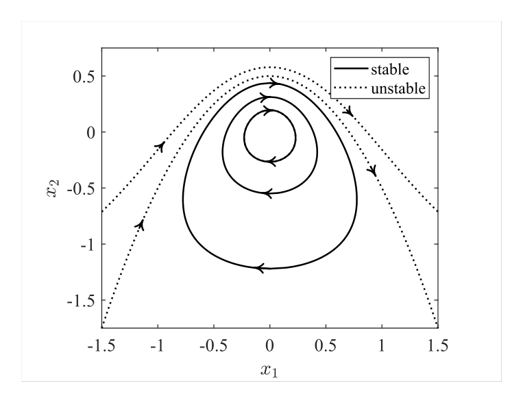

The phase portraits of the original system in Eq. 21 are shown in Fig. 1. A first integral of the unknown system is
| (22) |
The stability of the system depends on the initial condition . When the initial condition is such that the constant , the system is stable and the positive orbit itself is the invariant manifold . The manifold is a smooth, one dimensional, regularly embedded submanifold in the phase space . In this example, we choose the trajectory for of which the constant in Eq. 22. The samples are taken uniformly along the manifold with respect to the intrinsic metric of the manifold . Although in practice, such sampling procedure cannot be accomplished without knowing the manifold a priori, it is not difficult to picture that as , the set gradually fills the manifold . The samples are used to construct the approximant RKHS . The Sobolev-Mateŕn kernel is used to induce the RKHS. The subscript denotes the order of the kernel. If , then all the functions in the RKHS induced by over also belong to every Sobolev space where [24]. The general expression of is defined using a Bessel function, but when the kernel has the following closed-form expressions
where , and is the scaling factor of length [32].
Fig. 2 shows the contour of the estimation error in using when and . The result is as expected. The estimate of error in the unknown function is close to zero along the manifold . The rate of convergence with respect to the number of samples is shown in Fig. 3-4. Note that the manifold is a closed curve, and the samples are taken uniformly in metric. As a result, the fill distance . With this in mind, by Corollary 2 we have the following relationship
In this example, the set is PE, so over . The RKHS where . Thus the space of restrictions , and . On the other hand, we must have so that . In this way, we have
From the analysis above, we obtain the rates of convergence for the -norm. When , the order . When , the order . Taking the logarithms for both sides of the equation above, the values calculated above are the worst case of slope bounds in Fig. 3-4. In both figures, the actual error curves are below the slope bounds, which validates the conclusions in Corollary 2. One assumption for the Theorem 1 to hold is that must be smaller than a threshold. This assumption may explain the flat error curve when .
V Conclusions
The RKHS embedding method constructs estimates of the unknown or uncertain functions that appear in types of ODEs in an infinite dimensional RKHS. This paper considers the practical problem of formulating finite dimensional approximations for this technique. The convergence of approximations is proven, and the rates of convergence are derived. By selecting the reproducing kernel that has algebraic decaying Fourier transform, the induced RKHS is embedded in or equivalent to a standard Sobolev space. The error equation of approximation is recast in the Sobolev space, and bounds on the error of interpolation in Sobolev spaces are applied to analyse the error of approximation. When the trajectory of the unknown system concentrates in a compact, regularly embedded submanifold of the state space, the rate of convergence for finite dimensional approximation is derived in terms of the fill distance of the samples. It is shown that as the samples becomes increasingly dense in the submanifold, the approximation error decays accordingly.
References
- [1] S. Klus, F. Nüske, P. Koltai, H. Wu, I. Kevrekidis, C. Schütte, and F. Noé, “Data-driven model reduction and transfer operator approximation,” Journal of Nonlinear Science, vol. 28, no. 3, pp. 985–1010, 2018.
- [2] S. Pan and K. Duraisamy, “Data-driven discovery of closure models,” SIAM Journal on Applied Dynamical Systems, vol. 17, no. 4, pp. 2381–2413, 2018.
- [3] H. Liu, L. Zeng, W. Zhou, and S. Zhu, “A real-time data-driven control system for multi-motor-driven mechanisms,” International Journal of Robotics and Automation, vol. 32, no. 6, 2017.
- [4] D. Giannakis, “Data-driven spectral decomposition and forecasting of ergodic dynamical systems,” Applied and Computational Harmonic Analysis, vol. 47, no. 2, pp. 338–396, 2019.
- [5] Z. Drmac, I. Mezic, and R. Mohr, “Data driven modal decompositions: analysis and enhancements,” SIAM Journal on Scientific Computing, vol. 40, no. 4, pp. A2253–A2285, 2018.
- [6] S. Macesic, N. Crnjaric-Zic, and I. Mezic, “Koopman operator family spectrum for nonautonomous systems-part 1,” arXiv preprint arXiv:1703.07324, 2017.
- [7] E. M. Bollt, Q. Li, F. Dietrich, and I. Kevrekidis, “On matching, and even rectifying, dynamical systems through koopman operator eigenfunctions,” SIAM Journal on Applied Dynamical Systems, vol. 17, no. 2, pp. 1925–1960, 2018.
- [8] Q. Li, F. Dietrich, E. M. Bollt, and I. G. Kevrekidis, “Extended dynamic mode decomposition with dictionary learning: A data-driven adaptive spectral decomposition of the koopman operator,” Chaos: An Interdisciplinary Journal of Nonlinear Science, vol. 27, no. 10, p. 103111, 2017.
- [9] M. Korda and I. Mezić, “On convergence of extended dynamic mode decomposition to the koopman operator,” Journal of Nonlinear Science, vol. 28, no. 2, pp. 687–710, 2018.
- [10] S. L. Brunton and J. N. Kutz, Data-driven science and engineering: Machine learning, dynamical systems, and control. Cambridge University Press, 2019.
- [11] J. A. Farrell and M. M. Polycarpou, Adaptive approximation based control: unifying neural, fuzzy and traditional adaptive approximation approaches. John Wiley & Sons, 2006, vol. 48.
- [12] Y. Zhao and J. A. Farrell, “Self-organizing approximation-based control for higher order systems,” IEEE Transactions on Neural Networks, vol. 18, no. 4, pp. 1220–1231, 2007.
- [13] C. L. P. Chen, G. X. Wen, Y. J. Liu, and Z. Liu, “Observer-based adaptive backstepping consensus tracking control for high-order nonlinear semi-strict-feedback multiagent systems,” IEEE Transactions on Cybernetics, vol. 46, no. 7, pp. 1591–1601, 2016.
- [14] O. San, R. Maulik, and M. Ahmed, “An artificial neural network framework for reduced order modeling of transient flows,” Communications in Nonlinear Science and Numerical Simulation, vol. 77, pp. 271–287, 2019.
- [15] M. Chen, P. Shi, and C. C. Lim, “Adaptive neural fault-tolerant control of a 3-dof model helicopter system,” IEEE Transactions on Systems Man Cybernetics-Systems, vol. 46, no. 2, pp. 260–270, 2016.
- [16] L. Györfi, M. Kohler, A. Krzyzak, and H. Walk, A distribution-free theory of nonparametric regression. Springer Science & Business Media, 2006.
- [17] P. Bobade, S. Majumdar, S. Pereira, A. J. Kurdila, and J. B. Ferris, “Adaptive estimation in reproducing kernel hilbert spaces,” in 2017 American Control Conference (ACC). IEEE, 2017, pp. 5678–5683.
- [18] ——, “Adaptive estimation for nonlinear systems using reproducing kernel hilbert spaces,” Advances in Computational Mathematics, vol. 45, no. 2, pp. 869–896, 2019.
- [19] P. Bobade, D. Panagou, and A. J. Kurdila, “Multi-agent adaptive estimation with consensus in reproducing kernel hilbert spaces,” in 2019 18th European Control Conference (ECC). IEEE, 2019, pp. 572–577.
- [20] A. Kurdila and Y. Lei, “Adaptive control via embedding in reproducing kernel hilbert spaces,” in 2013 American Control Conference. IEEE, 2013, pp. 3384–3389.
- [21] A. J. Kurdila and P. Bobade, “Koopman theory and linear approximation spaces,” arXiv preprint arXiv:1811.10809, 2018.
- [22] J. Guo, S. T. Paruchuri, and A. J. Kurdila, “Persistence of excitation in uniformly embedded reproducing kernel hilbert (rkh) spaces,” arXiv preprint arXiv:2002.07963, 2020.
- [23] P. Bobade, D. Panagou, and A. J. Kurdila, “Multi-agent adaptive estimation with consensus in reproducing kernel hilbert spaces,” in 2019 18th European Control Conference (ECC). IEEE, 2019, pp. 572–577.
- [24] E. Fuselier and G. B. Wright, “Scattered data interpolation on embedded submanifolds with restricted positive definite kernels: Sobolev error estimates,” SIAM Journal on Numerical Analysis, vol. 50, no. 3, pp. 1753–1776, 2012.
- [25] T. Hangelbroek, F. J. Narcowich, and J. D. Ward, “Kernel approximation on manifolds i: bounding the lebesgue constant,” SIAM Journal on Mathematical Analysis, vol. 42, no. 4, pp. 1732–1760, 2010.
- [26] T. Hangelbroek, F. J. Narcowich, X. Sun, and J. D. Ward, “Kernel approximation on manifolds ii: The norm of the projector,” SIAM journal on mathematical analysis, vol. 43, no. 2, pp. 662–684, 2011.
- [27] A. Berlinet and C. Thomas-Agnan, Reproducing kernel Hilbert spaces in probability and statistics. Springer Science & Business Media, 2011.
- [28] R. A. Adams and J. J. Fournier, Sobolev spaces. Elsevier, 2003.
- [29] E. Zeidler and L. F. Boron, Nonlinear Functional Analysis and Its Applications: II/ A: Linear Monotone Operators. Springer, 1989.
- [30] F. Narcowich, J. Ward, and H. Wendland, “Sobolev bounds on functions with scattered zeros, with applications to radial basis function surface fitting,” Mathematics of Computation, vol. 74, no. 250, pp. 743–763, 2005.
- [31] R. Arcangéli, M. C. L. de Silanes, and J. J. Torrens, “An extension of a bound for functions in sobolev spaces, with applications to (m, s)-spline interpolation and smoothing,” Numerische Mathematik, vol. 107, no. 2, pp. 181–211, 2007.
- [32] C. E. Rasmussen, “Gaussian processes in machine learning,” in Summer School on Machine Learning. Springer, 2003, pp. 63–71.