Submodular Meta-Learning
Abstract
In this paper, we introduce a discrete variant of the Meta-learning framework. Meta-learning aims at exploiting prior experience and data to improve performance on future tasks. By now, there exist numerous formulations for Meta-learning in the continuous domain. Notably, the Model-Agnostic Meta-Learning (MAML) formulation views each task as a continuous optimization problem and based on prior data learns a suitable initialization that can be adapted to new, unseen tasks after a few simple gradient updates. Motivated by this terminology, we propose a novel Meta-learning framework in the discrete domain where each task is equivalent to maximizing a set function under a cardinality constraint. Our approach aims at using prior data, i.e., previously visited tasks, to train a proper initial solution set that can be quickly adapted to a new task at a relatively low computational cost. This approach leads to (i) a personalized solution for each task, and (ii) significantly reduced computational cost at test time compared to the case where the solution is fully optimized once the new task is revealed. The training procedure is performed by solving a challenging discrete optimization problem for which we present deterministic and randomized algorithms. In the case where the tasks are monotone and submodular, we show strong theoretical guarantees for our proposed methods even though the training objective may not be submodular. We also demonstrate the effectiveness of our framework on two real-world problem instances where we observe that our methods lead to a significant reduction in computational complexity in solving the new tasks while incurring a small performance loss compared to when the tasks are fully optimized.
1 Introduction
Many applications in artificial intelligence necessitate exploiting prior data and experience to enhance quality and efficiency on new tasks. This is often manifested through a set of tasks given in the training phase from which we can learn a model or representation that can be used for new unseen tasks in the test phase. In this regard, Meta-learning aims at exploiting the data from the available tasks to learn model parameters or representation that can be later used to perform well on new unseen tasks, in particular, when we have access to limited data and computational power at the test time thrun2012learning; schmidhuber1992learning; bengio1990learning; vilalta2002perspective. By now, there are several formulations for Meta-learning, but perhaps one of the most successful ones is the Model-Agnostic Meta-Learning (MAML) finn2017model. In MAML, we aim to train the model parameters such that applying a few steps of gradient-based updates with a small number of samples from a new task would perform well on that task. MAML can also be viewed as a way to provide a proper initialization, from which performance on a new task can be optimized after a few gradient-based updates. Alas, this scheme only applies to settings in which the decision variable belongs to a continuous domain and can be adjusted using gradient-based methods at the test time.
Our goal is to extend the methodology of MAML to the discrete setting. We consider a setting that our decision variable is a discrete set, and our goal is to come up with a good initial set that can be quickly adjusted to perform well over a wide range of new tasks. In particular, we focus on submodular maximization to represent the tasks which is an essential class of discrete optimization.
There are numerous applications where the submodular meta-learning framework can be applied to find a personalized solution for each task while significantly reducing the computation load. In general, most recommendation tasks can be cast as an instance of this settinggabillon2013adaptive; el2009turning; yue2011linear. Consider the task of recommending a set of items, e.g., products, locations, ads, to a set of users. One approach for solving such a problem is to find the subset of items that have the highest score over all the previously-visited users and recommend that subset to a new user. Indeed, this approach leads to a reasonable performance at test time; however, it does not provide a user-specific solution for a new user. Another approach is to find the whole subset at the test time when the new user arrives. In contrast to the previous approach, this scheme leads to a user-specific solution, but at the cost of running a computationally expensive algorithm to select all the elements at the test time.
In our Meta-learning framework, the process of selecting set items to be recommended to a new user is done in two parts: In the first part, a set of items are selected offline according to prior experience. These are the most popular items to the previously-visited users (depending on the context). In the second part, which happens at the test time, a set of items that is personalized to the coming user is selected. These are items that are computed specifically according to the features of the coming user. In this manner, the computation for each coming user would be reduced to the selection of the second part, which typically constitutes a small portion of the final set of recommended items. The first part can be done offline with a lower frequency. For instance, in a real recommender system, the first part can be computed once every hour, and the second part can be computed specifically for each coming user (or for a class of similar users). While we have mentioned recommendation (or more generally facility location) as a specific example, it is easy to see that this framework can be easily used to reduce computation in other notable applications of submodular optimization.
Contributions. Our contributions are threefold:
- •
We propose a novel discrete Meta-learning framework where each task is equivalent to maximizing a set function under some cardinality constraint. Our framework aims at using prior data, i.e., previously visited tasks, to train a proper initial solution set that can be quickly adapted to a new task at a low computational cost to obtain a task-specific solution.
- •
We present computationally efficient deterministic and randomized meta-greedy algorithms to solve the resulting meta-learning problem. When the tasks are monotone and submodular, we prove that the solution obtained by the deterministic algorithm is at least -optimal, and the solution of the randomized algorithm is -optimal in expectation, where the term vanishes by the size of the solution. These guarantees are obtained by introducing new techniques, despite that the meta-learning objective is not submodular.
- •
We study the performance of our proposed meta-learning framework and algorithms for movie recommendation and ride-sharing problems. Our experiments illustrate that the solution of our proposed meta-learning scheme, which chooses a large portion of the solution in the training phase and a small portion adaptively at test time, is very close to the solution obtained by choosing the entire solution at the test time when a new task is revealed.
1.1 Related work
Continuous Meta-Learning. Meta-learning has gained considerable attention recently mainly due to its success in few shot learning vinyals2016matching; DBLP:conf/iclr/RaviL17; snell2017prototypical; wang2019few as well as reinforcement learning DBLP:journals/corr/DuanSCBSA16; wang2016learning; DBLP:conf/iclr/SongGYCPT20. One of the most successful forms of meta-learning is the gradient-based Model Agnostic Meta-learning (MAML) approachfinn2017model. MAML aims at learning an initialization that can be adapted to a new task after performing one (or a few) gradient-based update(s); see, e.g., fallah2019convergence. This problem can be written as
| (1) |
where is the feasible set and is the probability distribution over tasks. The previous works on MAML including nichol2018first; finn2018probabilistic; DBLP:conf/iclr/GrantFLDG18; yoon2018bayesian; DBLP:conf/iclr/AntoniouES19; fallah2019convergence; collins2020distribution consider the case where is a continuous space. In fact none of these works can be applied to the case where the feasible parameter space is discrete. In this paper, we aim to close this gap and extend the terminology of MAML to discrete settings.
Submodular Maximization. Submodular functions have become key concepts in numerous applications such as data summarization lin2011class; wei2013using; kirchhoff2014submodularity; mirzasoleiman2016distributed, viral marketing kempe2003maximizing, sensor placement krause2008near, dictionary learning das2011submodular, and influence maximization kempe2003maximizing. It is well-known that for maximizing a monotone and submodular function under the cardinality constraint, the greedy algorithm provides a -optimal solution krause2014submodular; nemhauser1978best; wolsey1982analysis. There has been significant effort to improve the scalability and efficiency of the greedy algorithm using lazy, stochastic, and distributed methods mirzasoleiman2015lazier; karimi2017stochastic; barbosa2015power; mirrokni2015randomized; kumar2015fast; balkanski2019exponential. However, our framework is fundamentally different and complementary to these approaches as it proposes a new approach to use data at training time to improve performance at new tasks. Indeed, all the aforementioned techniques can be readily used to further speed-up our algorithms. Optimization of related submodular tasks has been a well-studied problem with works on structured prediction lin2012learning, submodular bandits yue2011linear; zhang2019online, online submodular optimization jegelka2011online; streeter2009online; chen2018projection, and public-private data summarization mirzasoleiman2016fast. However, unlike our work, these approaches are not concerned with train-test phases for optimization. Another recently-developed methodology to reduce computation is the two-stage submodular optimization framework balkanski2016learning; mitrovic2018data; stan2017probabilistic, which aims at summarizing the ground set to a reasonably small set that can be used at test time. The main difference of our framework with the two-stage approaches is that we allow for personalization: A small subset of items that can be found at test time specific to the task at hand. This leads to a completely new problem formulation, and consequently, new algorithms (more details in the supplementary material).
2 Problem Statement: Discrete Meta-Learning
Setup. We consider a family of tasks , where the set could be of infinite size. Each task is represented via a set function that measures the reward of a set for the -th task, and performing the task would mean to maximize the function subject to a given constraint. For instance, in a recommender system where we aim to recommend a subset of the items to the users, the set denotes the set of all the possible users and selecting which items to recommend to a user is viewed as the task . Moreover, the function encodes the users satisfaction, i.e., quantifies how suitable the set of items is for user . Taking a statistical perspective, we assume that the tasks occur according to a possibly unknown probability distribution .
In this paper, we focus on the case where the functions are monotone and submodular set functions and each task amounts to maximizing under the -cardinality constraint. That is, the task is to select a subset of size such that the value of is maximized. Submodularity of means that for any we have . Furthermore, is called monotone if for any we have .
Training and test tasks. We assume access to a collection of training tasks . These are the tasks that we have already experienced, i.e., they correspond to the users that we have already seen. Formally, this means that for each training task , we assume knowledge of the corresponding function . In our formulation, each of the training tasks is assumed to be generated i.i.d. according to the distribution . Indeed, eventually we aim to optimize performance at test time, i.e., obtain the best performance for new and unseen tasks generated independently from the distribution . For instance, in our recommendation setting, test tasks correspond to new users that will arrive in the future. Our goal is to use the training tasks to reduce the computation load at test time.
Two extremes of computation. Let us use (and ) to denote the task (and its corresponding set function) that we aim to learn at test time. Ideally, if we have sufficient computational power, then we should directly optimize by solving the following problem
| (2) |
We denote the optimal solution of (2) by . For instance, we can use the greedy procedure to solve (2) which leads to a -optimal solution using evaluations of , and through passes over the ground set. However, the available computational power and time in the test phase is often limited, either because we need to make quick decisions to respond to new users or since we need to save energy. For instance, in real-world advertising or recommendation systems, both these requirements are crucial: many users arrive within each hour which means fast optimization is crucial (especially if are large), and also, reducing computation load would lead to huge energy savings in the long run. In such cases, Problem (2) should be solved approximately with less computation.
An alternative to reduce computation at test time is to solve the problem associated with the expected reward over all possible tasks in the training phase (when we have enough computation time), i.e.,
| (3) |
We denote the optimal solution of (3) by . The rationale behind this approach is that the optimal solution to this problem would generalize well over an unseen task if the new task is also drawn according to the probability distribution . In other words, the solution of (3) should perform well for the problem in (2) that we aim to solve at the test time, assuming that is sampled according to . In this way, we do not need any extra computation at the test time. However, in this case, the solution that we obtain would not be the best possible solution for the task that we observe at the test time, i.e., is not equal to . As we often do not have access to the underlying probability distribution , and we only have access to a large set of realizations of tasks in the training phase. As a result, instead of solving (3), we often settle for maximizing the sample average function
| (4) |
where is the number of available tasks in the training phase.
Problems (2) and (4) can be considered as two different extreme cases. In the first option, by solving (2), we avoid any pre-processing in the training phase, and we obtain the best possible guarantee for the new task, but at the cost of performing computationally expensive operations (e.g., full greedy) at the test time. In the second approach, by solving (4) in the training phase, we obtain a solution that possibly performs reasonably without any computation at the test phase, but the quality of the solution may not be as good as the first option. In summary, there exists a trade-off between the required computational cost at the test time and the performance guarantee on the unseen task. Hence, a fundamental question that arises is what would be the best scheme at the training phase assuming that at test time we have some limited computational power. For instance, in the monotone submodular case, assume that instead of running the greedy algorithm for rounds, which has a complexity , we can only afford to run rounds of greedy at test time, which has complexity , where is small. In this case, a natural solution would be to find an appropriate set of elements in the training phase, and add the remaining elements at test time when a new task arrives. This discussion also applies to any other greedy method (e.g., lazy or stochastic greedy).
Discrete Meta-Learning. As we discussed so far, when computational power is limited at test time, it makes sense to divide the process of choosing the best decision between training and test phases. To be more specific, in the training phase, we choose a subset of elements from the ground set that would perform over the training tasks, and then select (or optimize) the remaining elements at the test time specifically with respect to the task at hand. To state this problem, consider with cardinality , where , as the initial set that we aim to find at the training phase, and the set that we add to the initial set at test time (See Figure 1 for an illustration). Hence, the problem of interest can be written as
| (5) |
Note that the critical decision variable that we need to find is which is the best initial subset of size overall all possible choices of task when a best subset of size is added to that. In fact, if we define , then we can rewrite the problem in (5) as
| (6) |
As described previously, we often do not have access to the underlying probability distribution of the tasks, and we instead have access to a large number of sampled tasked that are drawn independently according to . Hence, instead of solving (5), we solve its sample average approximation given by
| (7) |
where is the number of tasks in the training set which are sampled according to . Even though the functions are submodular, is not submodular or -submodular ohsaka2015monotone (see the supplementary materials for specific counter examples). Hence, Problem (7) is not a submodular maximization problem. In the next section, we present algorithms for solving Problem (7) with provable guarantees.
We finally note that Problem (7) will be solved at training time to find the solution of size . This solution is then completed at test time, by e.g. running further rounds of greedy on the new task, to obtain a task-specific solution of size .
3 Algorithms for Discrete Submodular Meta-Learning
Solving Problem (7) requires finding a set for the outer maximization and sets for the inner maximization. In this section, we describe our proposed greedy-type algorithms to select the elements and . As we deal with sets, the order in which the sets and are updated becomes crucial, i.e., it is not clear which of the sets or ’s should be preferably updated in each round and how can the functions be incorporated in finding the right order, which is the main challenge in designing greedy methods to solve (7). We design greedy procedures with both deterministic and randomized orders and provide strong guarantees for their solutions.
3.1 Deterministic Algorithms
In this section, we first describe Algorithms 1 and 2 which use specific orderings to solve Problem (7). Based on these two, we then design Algorithm 3 as our main deterministic algorithm. Throughout this section, we use to denote the marginal gain of adding an element to set for function . In brief, Algorithm 1 first fills greedily up to completion and then it constructs each of the ’s greedily on the top of . Specifically, starting from the empty set initialization for and ’s, Algorithm 1 constructs in its first phase the set in rounds, by adding one element per round, where the next element in each round is chosen according to . Once is completed, in the second phase, each of the sets is constructed in parallel by running the greedy algorithm on . That is, each is updated in rounds where in each round an element with maximum marginal on is added to based on .
Algorithm 2 uses the opposite ordering of Algorithm 1. Initializing with all sets to be empty, in the first phase it constructs the sets using the greedy procedure on , i.e., each is updated in parallel in rounds, where in each round the element is added to . In the second phase, the set is formed greedily in rounds, and in each round the following element is added .
While the solutions obtained by Algorithms 1 and 2 are guaranteed to be near-optimal, it turns out that they can be complementary with respect to each other. Our main deterministic algorithm, called Meta-Greedy, runs both Algorithms 1 and 2 and chooses as output the solution, among the two, that leads to a higher objective value in (7). Next, we explain why our Meta-Greedy method can outperform both Algorithms 1 and 2. This will be done by providing the theoretical guarantees for these methods and consequently explaining why Algorithms 1 and 2 are complementary.
Theoretical guarantees. We begin with the analysis of Algorithm 1. The following proposition relates the overall performance of Algorithm 1 to its performance after phase 1 and shows that the output of the algorithm is at least -optimal. We use OPT for the optimal value of Problem (7).
Proposition 1.
The proof of this proposition is relegated to the supplementary material. The key step in the proof is to relate the progress made in phase 1 to the gap to OPT. This is indeed challenging as phase 1 only involves updates on the outer maximization of (7). In this regard, we prove a novel technical lemma that can be generally applicable to any mini-max submodular problem. The guarantee given in Proposition 1 is minimized when . If is small (e.g., ) or if is large (e.g. if ) then the guarantee becomes tight (e.g. . This is indeed expected from the greedy nature of the two phases of Algorithm 1. What is non-trivial about the result of Proposition 1 is that it provides a strong guarantee for any value of , and not just cases that is small or large. Similarly, we can provide near-optimality guarantees for Algorithm 2.
Proposition 2.
Similarly, we can show that leads to (the worst) guarantee -OPT, while for large and small values of the bound in Proposition 2 approaches the optimal approximation .
We note that the values in Proposition 1 (Algorithm 1) and in Proposition 2 (Algorithm 2) represent two different extremes. The value represents how significant is the role of the set in solving Problem (7), and represents how significant the role of the sets can be. Even though the worst-case guarantees of Propositions 1 and 2 are obtained when , a coupled analysis of the algorithms show that in this case at least one of the algorithms should output a solution which is strictly better than -optimal. In other words, the outcomes of Algorithms 1 and 2 are dependent to one another, and the best performance is achieved when the maximum of the two is considered. This justifies why our main algorithm Meta-Greedy can perform strictly better than each of the Algorithms 1 and 2. Using a coupled analysis of the outcome of Algorithms 1 and 2, we can bound the performance of Meta-Greedy for different values of and (see the proof of Theorem 1 in the supplementary materials). In particular, we can show that the output of Meta-Greedy is at least -optimal. The proof of the following theorem carefully analyzes the interplay between the role of the inner and outer maximization problems in (7). We emphasize that the proof introduces new techniques applicable to other types of minimax submodular problems.
Theorem 1.
Consider the Meta-Greedy algorithm outlined in Algorithm 3. If the functions are monotone and submodular, then we have
| (8) |
3.2 Randomized Algorithm
In this section, we consider greedy procedures in which the decision to alternate between the set (the outer maximization) and the sets (the inner maximization) is done based on a randomized scheme. The Randomized meta-Greedy procedure, outlined in Algorithm 4, provides a specific randomized order. In each round, with probability we choose to perform a greedy update on , and with probability we choose to perform a greedy update on all the ’s, . This procedure continues until either or hit their corresponding carnality constraint, in which case we continue to update the other set(s) greedily until they also become full.
The randomized update of Algorithm 4 is designed to optimally connect the expected increase the objective value at each round with the gap to OPT (as shown in the proof of Theorem 2). Hence, the Randomized meta-Greedy procedure is able to achieve in expectation a guarantee close to the tight value . However, due to the randomized nature of the algorithm, the sets or might hit their carnality constraint earlier than expected. Analyzing the function value at this “stopping time” is another technical challenge that we resolve in the following theorem to obtain a guarantee that becomes slightly worse than depending on the values and .
Theorem 2.
Let the (random) sets , be the output of Algorithm 4. If the functions are monotone and submodular, then
where as and grow. More precisely, we have and
Remark 1.
All presented algorithms are designed for the training phase and their output is the set with size . The sets are only computed for algorithmic purposes. Given a new task at the test phase, the remaining task-specific elements will be added to using e.g. greedy updates that require a total complexity of in function evaluations. Also, the training complexity of the proposed algorithms is , however, certain phases can be implemented in parallel.
4 Simulation Results
We provide two experimental setups to evaluate the performance of our proposed algorithms and compare with other baselines. Each setup involves a different set of tasks which are represented as submodular maximization problems subject to the -cardinality constraint. We have considered the following algorithms: Meta-Greedy (Algorithm 3), Randomized Meta-Greedy (Algorithm 4), Greedy-Train (which chooses all the elements during the training phase–see (4) and the discussion therein), Greedy-Test (which chooses all the elements during the test phase–see (2) and the discussion therein), and Random (which chooses a random set of elements). In the following, we briefly explain the data and tasks and refer the reader to the supplementary materials for more details.
Ride Share Optimization. We will formalize and solve a facility location problem on the Uber dataset uber_2019. Our experiments were run on the portion of data corresponding to Uber pick-ups in Manhattan in the period of September 2014. This portion consists of data points each represented as a triplet . A customer and a driver are specified through their locations on the map. We use for a customer a and for a driver. We define the “convenience score” of a (customer, driver) pair as , where denotes the Manhattan distance mitrovic2018data. Given a specific time , we define a time slot and picking inside the data set 10 points in half an hour prior to time , and for each point we further pick 10 points in its 1 km neighborhood, which makes a total of 100 points (locations) on the map. A task , takes place at a corresponding time , and by defining the set of locations as above, we let be a monotone submodular function defined over a set of driver locations as . We pick 100,000 locations at random from the September 2014 Uber pick-up locations as a ground set. For training we form tasks by picking for each task a random time in the first week of Sept. 2014. We test on new tasks formed similarly from the second week of Sept. 2014 and report in the figures the average performance obtained at test tasks.
Figures 2(a) and 2(b) show the performance of our proposed algorithms against the baselines mentioned above. Figure (2(a)) shows the performance of all algorithms when we fix , and vary from 5 to 18. Larger means less computation at test time (since we need to further choose elements at test). However, we see that even for large values of (e.g. ), the performance of Meta-Greedy is still quite close to the ideal performance of Greedy-Test. Putting this together with the fact that the performance of Greedy-Train is not so good, we can conclude that adding a few personalized elements at test time significantly boosts performance to be even close to the ideal. In Figure (2(b)), we compare the performance of all the algorithms when changes from 5 to 30, and is of (). As we can see, even when we just learn of the set in test time, the performance of Meta-greedy is close to Test-Greedy. Also, when increases, Random-Meta-Greedy performs better than Meta-Greedy. This is in compliance with the results of Theorems 1, 2.


Movie Recommendation. In this application, we use the Movielens dataset harper2015movielens which consists of ratings (from 1 to 5) by users for movies. We pick the 2000 most rated movies, and 200 users who rated the highest number of movies (similar to stan2017probabilistic). We partitioned the 200 users into 100 users for the training phase and 100 other users for the test phase. Each movie can belong to one of 18 genre. For each genre we let be the set of all movies with in genre . For each user , we let be the set of all movie rated by the user, and for each movie the corresponding rating is denoted by . Furthermore, for user we define which is the weighted average over maximum rate that user gives to movies from each genre and is proportion of movies in genre which is rated by user out of all the rating he provides. A task involves 5 users and the function assigned to the task is the average of . We formed training tasks from the users in the training phase, and test tasks from the users in the test phase. Figure (2(c)) (resp. 2(d)) has been obtained in a similar format as Figure 2(a) (resp. Figure 2(b)). Indeed, we observe a very similar pattern as in the rideshare experiments.

Comparison with Two-stage Submodular Optimization. Two-stage submodular optimization is another way to deal with limited computational power in test time. In this framework, at the training time, a reduced ground set will be learned which will be used as a ground set at test time. This procedure will reduce the computational time in the test time. More formally, the two-stage submodular optimization framework aims to solve the following problem: Let for , be a monotone submodular function over ground set . The goal is to find with size at most whose subests of size maximize the sum of for :
| (9) |
Once the set is found, it will be used at the test time (e.g. by running full greedy on as the reduced ground set) to find elements for a new task. Although this framework uses function evaluations for each new test task, however, it poorly personalizes to a test task because the set has been optimized only for the tasks at the training time. This intuition is indeed consistent with our experimental findings reported below. We further remark that the two-stage framework needs high computational power in training; Hence, we were not able to run the state-of-the-art two-stage algorithms to solve (9) in the setting considered in our main simulation results, e.g., for a ground set of size the implementation of two-stage approach would take a very long time.
We consider the ride-sharing application and let (ground set size), (number of tasks), and changing from 5 to 30 (cardinality constraint) while (portion that will fill in the submodular meta-learning during training), and (size of reduced ground set for two-stage framework). For solving the two-stage problem (9) we have used the Replacement-Greedy algorithm introduced in stan2017probabilistic. We choose these parameters based on the following two facts: First, because of the high computational cost of the Replacement Greedy algorithm in training for the ride-sharing application, we chose to be 500. Second, we provide a fair comparison in terms of computational power at test time, which means both Meta-Greedy (our algorithm) and Replacement-Greedy have exactly the same computational cost at test time. Formally, .
we report the result for the above setting in the Figure 3. A few comments are in order: (i) The two stage implementation reduces the ground set of size to . When is small, some of the popular elements found at training time would be good enough to warrant a good performance at test time. However, when increases, the role of personalizing becomes more apparent. As we see, the performance of Replacement-Greedy does not improve much when we increase and it is close to the performance of Greedy-Train (which chooses all the elements during the training phase–see (4) and the discussion therein). However, since Meta-Greedy does (a small) task-specific optimization at test time, its performance becomes much better. We emphasize again that, in order to be fair, the comparison in Figure 3 has been obtained using the same computational power allowed at test time for both meta-learning and two-stage approaches.
Broader Impact
This paper introduces a discrete Meta-learning framework that aims at exploiting prior experience and data to improve performance on future tasks. While our results do not immediately lead to broader societal impacts, they can potentially lead to new approaches to reduce computation load and increase speed in latency-critical applications, such as recommender systems, autonomous systems, etc. In such applications, where there is a flow of new tasks arriving at any time requiring fast decisions, the available computational power and time is often limited either because we need to make quick decisions to respond to new users/tasks or since we need to save energy. For instance, in real-world advertising or recommendation systems, both these requirements are crucial: many users arrive within each hour which means fast decision-making is crucial, and also, reducing computation load would lead to huge energy savings in the long run. Our framework is precisely designed to address this challenge. Moreover, the framework introduced in this paper can potentially open new doors in the research field of discrete optimization.
Acknowledgments and Disclosure of Funding
The research of Arman Adibi and Hamed Hassani is supported by NSF award CPS-1837253, NSF CAREER award CIF 1943064, and Air Force Office of Scientific Research Young Investigator Program (AFOSR-YIP) under award FA9550-20-1-0111. The research of Aryan Mokhtari is supported by NSF Award CCF-2007668.
References
- (1) S. Thrun and L. Pratt, Learning to learn. Springer Science & Business Media, 2012.
- (2) J. Schmidhuber, “Learning to control fast-weight memories: An alternative to dynamic recurrent networks,” Neural Computation, vol. 4, no. 1, pp. 131–139, 1992.
- (3) Y. Bengio, S. Bengio, and J. Cloutier, Learning a synaptic learning rule. Citeseer.
- (4) R. Vilalta and Y. Drissi, “A perspective view and survey of meta-learning,” Artificial intelligence review, vol. 18, no. 2, pp. 77–95, 2002.
- (5) C. Finn, P. Abbeel, and S. Levine, “Model-agnostic meta-learning for fast adaptation of deep networks,” in Proceedings of the 34th International Conference on Machine Learning-Volume 70, pp. 1126–1135, JMLR. org, 2017.
- (6) V. Gabillon, B. Kveton, Z. Wen, B. Eriksson, and S. Muthukrishnan, “Adaptive submodular maximization in bandit setting,” in Advances in Neural Information Processing Systems, pp. 2697–2705, 2013.
- (7) K. El-Arini, G. Veda, D. Shahaf, and C. Guestrin, “Turning down the noise in the blogosphere,” in Proceedings of the 15th ACM SIGKDD international conference on Knowledge discovery and data mining, pp. 289–298, 2009.
- (8) Y. Yue and C. Guestrin, “Linear submodular bandits and their application to diversified retrieval,” in Advances in Neural Information Processing Systems, pp. 2483–2491, 2011.
- (9) O. Vinyals, C. Blundell, T. Lillicrap, D. Wierstra, et al., “Matching networks for one shot learning,” in Advances in neural information processing systems, pp. 3630–3638, 2016.
- (10) S. Ravi and H. Larochelle, “Optimization as a model for few-shot learning,” in 5th International Conference on Learning Representations, ICLR, 2017.
- (11) J. Snell, K. Swersky, and R. Zemel, “Prototypical networks for few-shot learning,” in Advances in neural information processing systems, pp. 4077–4087, 2017.
- (12) Y. Wang and Q. Yao, “Few-shot learning: A survey,” arXiv preprint arXiv:1904.05046, 2019.
- (13) Y. Duan, J. Schulman, X. Chen, P. L. Bartlett, I. Sutskever, and P. Abbeel, “Rl$ˆ2$: Fast reinforcement learning via slow reinforcement learning,” CoRR, vol. abs/1611.02779, 2016.
- (14) J. X. Wang, Z. Kurth-Nelson, D. Tirumala, H. Soyer, J. Z. Leibo, R. Munos, C. Blundell, D. Kumaran, and M. Botvinick, “Learning to reinforcement learn,” arXiv preprint arXiv:1611.05763, 2016.
- (15) X. Song, W. Gao, Y. Yang, K. Choromanski, A. Pacchiano, and Y. Tang, “ES-MAML: simple Hessian-free meta learning,” in 8th International Conference on Learning Representations, ICLR, 2020.
- (16) A. Fallah, A. Mokhtari, and A. Ozdaglar, “On the convergence theory of gradient-based model-agnostic meta-learning algorithms,” in International Conference on Artificial Intelligence and Statistics, pp. 1082–1092, 2020.
- (17) A. Nichol, J. Achiam, and J. Schulman, “On first-order meta-learning algorithms,” arXiv preprint arXiv:1803.02999, 2018.
- (18) C. Finn, K. Xu, and S. Levine, “Probabilistic model-agnostic meta-learning,” in Advances in Neural Information Processing Systems, pp. 9516–9527, 2018.
- (19) E. Grant, C. Finn, S. Levine, T. Darrell, and T. L. Griffiths, “Recasting gradient-based meta-learning as hierarchical bayes,” in 6th International Conference on Learning Representations, ICLR, 2018.
- (20) J. Yoon, T. Kim, O. Dia, S. Kim, Y. Bengio, and S. Ahn, “Bayesian model-agnostic meta-learning,” in Advances in Neural Information Processing Systems, pp. 7332–7342, 2018.
- (21) A. Antoniou, H. Edwards, and A. J. Storkey, “How to train your MAML,” in 7th International Conference on Learning Representations, ICLR, 2019.
- (22) L. Collins, A. Mokhtari, and S. Shakkottai, “Distribution-agnostic model-agnostic meta-learning,” arXiv preprint arXiv:2002.04766, 2020.
- (23) H. Lin and J. Bilmes, “A class of submodular functions for document summarization,” in Proceedings of the 49th Annual Meeting of the Association for Computational Linguistics: Human Language Technologies-Volume 1, pp. 510–520, Association for Computational Linguistics, 2011.
- (24) K. Wei, Y. Liu, K. Kirchhoff, and J. Bilmes, “Using document summarization techniques for speech data subset selection,” in Proceedings of the 2013 Conference of the North American Chapter of the Association for Computational Linguistics: Human Language Technologies, pp. 721–726, 2013.
- (25) K. Kirchhoff and J. Bilmes, “Submodularity for data selection in machine translation,” in Proceedings of the 2014 Conference on Empirical Methods in Natural Language Processing (EMNLP), pp. 131–141, 2014.
- (26) B. Mirzasoleiman, A. Karbasi, R. Sarkar, and A. Krause, “Distributed submodular maximization,” The Journal of Machine Learning Research, vol. 17, no. 1, pp. 8330–8373, 2016.
- (27) D. Kempe, J. Kleinberg, and É. Tardos, “Maximizing the spread of influence through a social network,” in Proceedings of the ninth ACM SIGKDD international conference on Knowledge discovery and data mining, pp. 137–146, 2003.
- (28) A. Krause, A. Singh, and C. Guestrin, “Near-optimal sensor placements in gaussian processes: Theory, efficient algorithms and empirical studies,” Journal of Machine Learning Research, vol. 9, no. Feb, pp. 235–284, 2008.
- (29) A. Das and D. Kempe, “Submodular meets spectral: Greedy algorithms for subset selection, sparse approximation and dictionary selection,” arXiv preprint arXiv:1102.3975, 2011.
- (30) A. Krause and D. Golovin, “Submodular function maximization..”
- (31) G. L. Nemhauser and L. A. Wolsey, “Best algorithms for approximating the maximum of a submodular set function,” Mathematics of operations research, vol. 3, no. 3, pp. 177–188, 1978.
- (32) L. A. Wolsey, “An analysis of the greedy algorithm for the submodular set covering problem,” Combinatorica, vol. 2, no. 4, pp. 385–393, 1982.
- (33) B. Mirzasoleiman, A. Badanidiyuru, A. Karbasi, J. Vondrák, and A. Krause, “Lazier than lazy greedy,” in Twenty-Ninth AAAI Conference on Artificial Intelligence, 2015.
- (34) M. Karimi, M. Lucic, H. Hassani, and A. Krause, “Stochastic submodular maximization: The case of coverage functions,” in Advances in Neural Information Processing Systems, pp. 6853–6863, 2017.
- (35) R. Barbosa, A. Ene, H. Nguyen, and J. Ward, “The power of randomization: Distributed submodular maximization on massive datasets,” in International Conference on Machine Learning, pp. 1236–1244, 2015.
- (36) V. Mirrokni and M. Zadimoghaddam, “Randomized composable core-sets for distributed submodular maximization,” in Proceedings of the forty-seventh annual ACM symposium on Theory of computing, pp. 153–162, 2015.
- (37) R. Kumar, B. Moseley, S. Vassilvitskii, and A. Vattani, “Fast greedy algorithms in mapreduce and streaming,” ACM Transactions on Parallel Computing (TOPC), vol. 2, no. 3, pp. 1–22, 2015.
- (38) E. Balkanski, A. Rubinstein, and Y. Singer, “An exponential speedup in parallel running time for submodular maximization without loss in approximation,” in Proceedings of the Thirtieth Annual ACM-SIAM Symposium on Discrete Algorithms, pp. 283–302, SIAM, 2019.
- (39) H. Lin and J. A. Bilmes, “Learning mixtures of submodular shells with application to document summarization,” arXiv preprint arXiv:1210.4871, 2012.
- (40) M. Zhang, L. Chen, H. Hassani, and A. Karbasi, “Online continuous submodular maximization: From full-information to bandit feedback,” in Advances in Neural Information Processing Systems, pp. 9210–9221, 2019.
- (41) S. Jegelka and J. A. Bilmes, “Online submodular minimization for combinatorial structures.,” in ICML, pp. 345–352, Citeseer, 2011.
- (42) M. Streeter and D. Golovin, “An online algorithm for maximizing submodular functions,” in Advances in Neural Information Processing Systems, pp. 1577–1584, 2009.
- (43) L. Chen, C. Harshaw, H. Hassani, and A. Karbasi, “Projection-free online optimization with stochastic gradient: From convexity to submodularity,” arXiv preprint arXiv:1802.08183, 2018.
- (44) B. Mirzasoleiman, M. Zadimoghaddam, and A. Karbasi, “Fast distributed submodular cover: Public-private data summarization,” in Advances in Neural Information Processing Systems, pp. 3594–3602, 2016.
- (45) E. Balkanski, B. Mirzasoleiman, A. Krause, and Y. Singer, “Learning sparse combinatorial representations via two-stage submodular maximization,” in International Conference on Machine Learning, pp. 2207–2216, 2016.
- (46) M. Mitrovic, E. Kazemi, M. Zadimoghaddam, and A. Karbasi, “Data summarization at scale: A two-stage submodular approach,” arXiv preprint arXiv:1806.02815, 2018.
- (47) S. Stan, M. Zadimoghaddam, A. Krause, and A. Karbasi, “Probabilistic submodular maximization in sub-linear time,” in Proceedings of the 34th International Conference on Machine Learning-Volume 70, pp. 3241–3250, JMLR. org, 2017.
- (48) N. Ohsaka and Y. Yoshida, “Monotone k-submodular function maximization with size constraints,” in Advances in Neural Information Processing Systems, pp. 694–702, 2015.
- (49) UberDataset, “Uber pickups in new york city.” https://www.kaggle.com/fivethirtyeight/uber-pickups-in-new-york-city.
- (50) F. M. Harper and J. A. Konstan, “The movielens datasets: History and context,” Acm transactions on interactive intelligent systems (tiis), vol. 5, no. 4, pp. 1–19, 2015.
Supplementary Material
5 Proof of Proposition 1
Let , be the output of Algorithm 1 and , be the optimal solution for problem (7). We first show that the output of algorithm 1 in phase 1 satisfies the following inequality:
| (10) |
To show (10) let be the element of greedy procedure in phase 1, and be the set in this procedure, where . let and define iteratively as follows. Let and define in the following way:
- 1.
If , then let .
- 2.
Otherwise, if , let be one of the elements of chosen uniformly at random.
Define .
We show this procedure in the following chain.
then we can write the following inequalities:
| (11) | ||||
| (12) | ||||
| (13) | ||||
| (14) | ||||
| (15) |
where (12) follows from definition of and the greedy procedure and (13) follows from submodularity since in each step and and finally, equation (14) follows from the fact that . Then, by summing over from 0 to we get the following inequality:
| (16) | ||||
| (17) | ||||
| (18) | ||||
| (19) |
where the last equality comes from the process of defining . Because, we only change one element by adding element found in greedy process and removing one element from the optimal set in each step and the size of is in each step; therefore, after step . By rearranging the terms and summing over the claim in (10) follows.
Second, for the phase 2 of the algorithm 1 we can use the usual analysis of greedykrause2014submodular for set :
| (20) | ||||
| (21) | ||||
| (22) |
where in the equation (20). Equation (20) follows from usual greedy analysis, equation (21) follows from definition of , and equation (22) follows from equation (10).
Finally, since by monotonicity . Then, combing this observation with the result in (22) implies
where
6 Proof of Proposition 2
Let , be the output of Algorithm 2 and , be the optimal solution for problem (7). We first show the following about the output of algorithm 2, phase 1.
| (23) |
to show (23) consider the following:
let . let and define iteratively as follows. Let and define in the following way:
- 1.
If , then ;
- 2.
Otherwise, if , let be one of the elements of chosen uniformly at random;
Define .
then we can write the following inequalities:
| (24) | ||||
| (25) | ||||
| (26) | ||||
| (27) | ||||
| (28) |
where (25) follows from definition of and the greedy procedure and (26) follows from the submodularity since in each step and and finally, equation (27) follows from the fact that because of monotonicity. Then, by summing over from 0 to we get the following inequality:
| (29) | ||||
| (30) | ||||
| (31) | ||||
| (32) |
where the last equality comes from the process of defining ; since, the size of is in each step and after step . Then, by rearranging and summing over we can obtain (23).
Second, for phase 2 of algorithm 2 we can use the usual analysis of greedykrause2014submodular for set :
| (33) | ||||
| (34) | ||||
| (35) |
where in equation (33). Equation (33) follows from the usual greedy analysis, equation (34) follows from the definition of , and equation (35) follows the from equation (23).
Finally, since by monotonicity . Then, combing (33)-(35) we have:
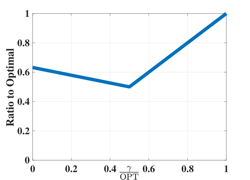
The following shows the ratio of lower bound to optimum (a similar plot can be obtained for the lower bound of Proposition 1 when is replaced with .).
7 Proof of Theorem 1
Let . Since found greedily given we can write:
| (36) |
for every . Also, we can write
| (37) | ||||
| (38) | ||||
| (39) | ||||
| (40) | ||||
| (41) |
where (40) comes from (36), and (41) comes from submodularity. We thus obtain
| (42) |
Also we can write for any set such that :
| (43) | ||||
| (44) | ||||
| (45) | ||||
| (46) | ||||
| (47) |
where (43) follows from submodularity, (45) follows from monotonicity, and (46) follows from (42), and (47) follows from (36). This results the following for any set such that :
| (48) |
Now, from (48) we can find a new bound for the performance of algorithm 3. From (48) we can write:
| (49) |
Also, since in Algorithm 1 the set is constructed greedily on the top of , we have:
| (50) | ||||
| (51) |
| (52) |
Using the same procedure as above, by defining , we can prove:
| (53) |
which results in the following lower bound:
| (54) |
Finally, given (52) and (54), the factor is obtained as a result of the following procedure. Let and given as and . Then the left-hand-side term in (8) is lower bounded by:
Note that the constraints hold due to the results of Proposition 1 and 2. In particular, the above bound is always larger than for any value of and .
8 Proof of Theorem 2
Consider round in which and the expected gain of the algorithm with probability is the maximum gain from adding an element or with probability the gain is which can be written as follows.
| (56) |
assuming is optimal solution, we can also write:
| (57) | ||||
| (58) | ||||
| (59) |
where (57) follows from monotonicity, and (58) follows from submodularity. Then, from (59) and (56) we conclude that:
| (60) |
In other words, the expected improvement in the objective (left-hand side of (60)) is at least times the gap of the current objective value to OPT (i.e. right-hand side of (60)). Note that (60) is only valid when and . Hence, by defining the stopping time as first time that either or , and a telescopic usages of the bounds in (60), we obtain the following bound:
The following theorem finds an upper bound on which finishes the proof.
Lemma 1.
If stopping time is first time that either or then where .
Proof.
let be random variables with distribution , i.e. . The stopping time is the first time that or . Let us define .
Furthermore, we define when is the first time that and when is the first time that . Also, let as it was defined in the lemma. By this definition, and we can write the following about the probabilities of and :
then, based on the definition of and we have the following properties for and :
- •
if then .
- •
if then .
- •
if then .
- •
if then .
- •
if then
- •
if then .
- •
.
- •
.
Moreover using Bayes rule we can write:
- •
- •
Let we can write where are random variable with distribution . Then, we can write the following using Chernoff bound:
| (61) | ||||
| (62) | ||||
| (63) | ||||
| (64) | ||||
| (65) |
Similarly:
| (66) | ||||
| (67) | ||||
| (68) | ||||
| (69) | ||||
| (70) | ||||
| (71) |
then we can write the as follows:
| (72) |
Our goal is to find proper bound for (72). we focus on the second term in (73)-(79) and try to find proper bound for it.
| (73) | ||||
| (74) | ||||
| (75) | ||||
| (76) | ||||
| (77) | ||||
| (78) | ||||
| (79) |
where (74) follows from law of total probability, (75) follows from bayes rule, (77) follows from Chernoff bound, (78) follows from the fact that . Let . As result, we have:
| (80) |
Assume without loss of generality and . As a result, . we want to show that . To show this, we show the following equivalent inequality :
| (81) |
This holds since we have . Moreover, we can bound the first term in (72) as follows:
| (82) |
summing up we can find the following bound for which finishes the proof.
| (83) |
∎
9 Counter-example for Submodularity of the Objective in (7)
In this section, we provide a counterexample for submodularity of the objective function in the equation (7). We consider a maximum coverage problem in which the function value is an area covered by a set of elements. We define the ground set which has shown in Figure 5. Each element is a rectangle, and a function value of that element is an area covered by that element. We refer to each element (rectangle) by it’s vertices.

Let , and . Also in (7) we let and which means that we are considering a single set function defined as: , where is a area of set . Note that the area function is monotone and submodular, however as we will show below, the function is not submodular. To do so, we consider two sets and and add the element to both sets and observe that does not satisfy the diminishing returns property. Let us first compute the function value at and as follows:
and
Similarly, we compute the function value at , and :
and
We can now see that , but . Therefore, is not submodular.
Also let us make a remark about -submodularity which studies functions of subsets of the ground set that are disjoint sets. This class of functions is submodular in each orthant ohsaka2015monotone. However, in the submodular meta-learning framework, sets can have overlap, and there is no restriction on the sets to be disjoint. Therefore, our framework is different from -submodular maximization.