跳到论文正文
W Papers独立论文阅读器 arXiv:2007.05571 论文正文 计算阅读时间 · 0%
引用这篇论文根据当前论文元数据生成,正式投稿前建议核对。


License: arXiv.org perpetual non-exclusive license
arXiv:2007.05571v1 [eess.SP] 10 Jul 2020

A New Frame Synchronization Algorithm for Linear Periodic Channels with Memory

Oren Kolaman       Ron Dabora   
Abstract

Identifying the start time of a sequence of symbols received at the receiver, commonly referred to as frame synchronization, is a critical task for achieving good performance in digital communications systems employing time-multiplexed transmission. In this work we focus on frame synchronization for linear channels with memory in which the channel impulse response is periodic and the additive Gaussian noise is correlated and cyclostationary. Such channels appear in many communications scenarios, including narrowband power line communications and interference-limited wireless communications. We derive frame synchronization algorithms based on simplifications of the optimal likelihood-ratio test, assuming the channel impulse response is unknown at the receiver, which is applicable to many practical scenarios. The computational complexity of each of the derived algorithms is characterized, and a procedure for selecting nearly optimal synchronization sequences is proposed. The algorithms derived in this work achieve better performance than the noncoherent correlation detector, and, in fact, facilitate a controlled tradeoff between complexity and performance.

Index Terms:
frame synchronization, cyclostationary signals, linear periodically time-varying channels, CMA equalizer, hypothesis testing, likelihood ratio test.

I Introduction

In digital communications, blocks of information bits are mapped into sequences of symbols taken from a finite constellation set. The transmitter partitions the stream of symbols into frames of finite duration, which are then sent to a receiver through a channel. In order for the receiver to successfully recover the information bits from the received distorted and noisy version of the transmitted signal, the receiver must first identify the physical parameters of the transmitted signal; In particular it has to first identify the starting time of a received frame before any subsequent processing task is applied. The process of identifying the beginning of a received information frame within a measured incoming stream of samples at the receiver is called frame synchronization (FS) [1], [2]. As an example, in time division multiple access (TDMA) systems, FS identifies the boundaries between the multiplexed users [3]. In the current work, the received signal consists of a convolution between the transmitted signal and a periodic channel impulse response (CIR), which generalizes upon the common linear time-invariant (LTI) channel model. Then, an additive cyclostationary Gaussian noise (ACGN) process with a finite correlation length is summed with the output of the convolution to form the overall received signal. The ACGN model generalizes upon the common additive stationary Gaussian noise model. The channel model described above represents many communications scenarios, including narrowband (NB) power line communications (PLC) and interference-limited wireless communications [4, Sec. 5], [5], [6]. Instances of these scenarios include non-orthogonal multiple access (NOMA) [7], [8], full duplex communications, cognitive communications [9], digital subscriber line (DSL) communications [10] as well as additional communications mediums and paradigms, including the “Internet of Things” [11]. In [6], we considered the joint estimation of the carrier frequency offset and the channel impulse response for this channel model, and proposed a compressed-sensing based approximate joint maximum likelihood estimator for these quantities. In this paper we study FS for the above received signal model, using the common pilot-assisted approach, in which the transmitted signal contains a specifically designed synchronization sequence which is embedded into the random data [1], [12]. Accordingly, the objective of the FS algorithm developed in this work is to identify the presence of the synchronization sequence within an observation window. The unique aspects of our work are the general channel model for which the algorithm is derived, as well as the rigorous approach used in the derivation, in contrast to the ad-hoc solutions of previous works. Novelty follows as previous works did not explicitly account for the channel memory in the derivation of the estimator, due to its associated computational complexity. Moreover, our derived algorithms do not assume knowledge of the CIR coefficients. To the best of our knowledge, an FS algorithm for an unknown linear channel with memory and ACGN, derived based on the likelihood ratio test (LRT) has not been previously presented.

The common approach for frame synchronization is the marker concept, in which a known synchronization sequence, also referred as the synchronization word (SW), is incorporated into each transmitted data frame, as conceptually

Refer to caption
Figure 1: The structure of transmitted frame. Overall, the frame contains Lf∈𝒩L_{\textsf{f}}\in\mathcal{N} complex symbols and is divided into two parts: A synchronization word whose length is Lsw∈𝒩L_{\textsf{sw}}\in\mathcal{N} and Ld=(Lf−Lsw)L_{\textsf{d}}=(L_{\textsf{f}}-L_{\textsf{sw}}) randomly selected data symbols denoted {dn}\{d_{n}\}.

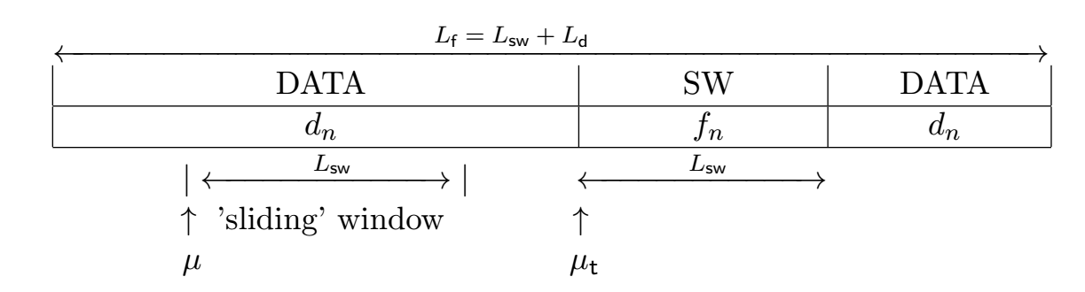
depicted in Fig 1. Assuming there is only one SW in each data frame, the synchronization algorithm observes the received signal and evaluates a mathematical function over a sliding search window whose duration is equal to the duration of the SW, as conceptually depicted in Fig. 2.
Refer to caption
Figure 2: Frame synchronization process: μt\mu_{\textsf{t}} is the true position of the synchronization sequence within the observation window and μ\mu is the start position of the sliding search window within the received observation window.

There are two main detection approaches which utilize the marker concept: The first approach evaluates a test metric for all possible positions within the observation window and chooses the start position of the SW as the value of μ\mu which maximizes the test metric. This approach is referred to as one-shot point estimation (OSPE) FS, [13, 14]. The second approach is comparing the test metric computed for a specific position μ\mu within the observation window to a pre-determined threshold, such that once the threshold value is exceeded, the start position of the synchronization sequence is declared. Otherwise, the test metric is evaluated at the next position. This approach is commonly referred to as sequential FS [13, 14]. A study of the theoretical and implementation tradeoffs between OSPE FS and sequential FS for the general problem of FS in the presence of a large residual carrier frequency offset, is reported in [13]. OSPE FS algorithms for memoryless additive white Gaussian noise (AWGN) channels have been proposed in [12, 15, 16, 17], and for AWGN channels with memory in [18] and [19]. In [12], Massey showed that the optimal rule, in the sense of maximizing the probability of correctly locating the SW, for OSPE FS over memoryless AWGN channels with coherent binary phase-shift keying (BPSK) transmission is a correlator between the synchronization sequence and the received signal, modified by an additive correction term which is a function of the received signal. In [15], the performance of the optimal detector presented in [12] is analyzed, and an explicit expression for the probability of synchronization error, leading to incorrect SW start position estimation within the data frame, is derived. It is observed in [15] that the performance of the high SNR approximate optimal detector derived in [12], is practically indistinguishable from the performance of the optimal detector. The work [16] extended [12] to a general MM-ary phase-coherent and phase-noncoherent signaling over AWGN channels. The work in [17] derived an OSPE FS algorithm for transmission of MM-ary symbols over memoryless AWGN channels with unknown phase and frequency offsets. In [18], the work of [12] was extended to AWGN intersymbol interference (ISI) channels with BPSK transmission assuming the CIR is known at the receiver. In [19], an algorithm for OSPE FS over AWGN channels with ISI unknown at the receiver, and with an arbitrary symbol constellation, was presented. The work of [19] first estimates the unknown CIR via a maximum likelihood estimation assuming an arbitrary location for the SW. Then, the estimated CIR is plugged back into the likelihood function to obtain the likelihood value for the assumed location, thus facilitating a search for the maximizing value of the location. This scheme was next extended to handle also unknown CFO.

Sequential FS algorithms over memoryless AWGN channels have been proposed in [20, 21, 22, 23, 14, 24]. The work in [14] developed a sequential FS algorithm for BPSK transmission over memoryless AWGN channels with an unknown noise variance and an unknown channel gain. The work in [20] presented a sequential FS algorithm based on hypothesis testing, for pilot-symbol assisted modulation (PSAM) transmission [25], in which the pilot and the data symbols are selected from disjoint sets, and the signal is received over a memoryless AWGN channel such that the channel gain has an unknown random phase and frequency offsets. In [21], an hypothesis testing-based optimal FS algorithm for BPSK transmission over AWGN channels was proposed using a SW. The work [21] assumed that the lengths of the frames are varying and are unknown at the receiver. The work in [22] extended the work of [21] to the case in which the probability distribution of the BPSK data symbols is unknown, which led to the derivation of a generalized likelihood ratio test (GLRT). In [24], a sequential FS algorithm was presented for BPSK transmission over memoryless AWGN channels, received with unknown random carrier phase offset. To the best of our knowledge, a sequential FS algorithm for channels with memory in which the CIR is unknown has not yet been derived, and this is the contribution of the current work.

Main Contributions: In this work we derive a sequential FS algorithm for channels with linear, periodically time-varying CIR and with ACGN, based on the likelihood ratio test (LRT) metric. The unique aspects of our work are the general channel model for which the algorithm is derived, as well as the rigorous approach used in the derivation, in contrast to the ad-hoc methods used in previous works. Novelty follows as previous works did not explicitly account for the channel memory in the derivation of the detector, due to its associated computational complexity. Moreover, our derived algorithm does not assume knowledge of the CIR coefficients. To the best of our knowledge, an FS algorithm for an unknown linear channel with memory and ACGN, derived based on the LRT has not been previously presented. Furthermore, in the proposed algorithm we apply approximations which facilitate a tradeoff between complexity and performance. The computational complexity of the proposed scheme is then explicitly derived. Lastly, we propose a statistics-based approach for constructing good SWs. We demonstrate the superiority of the proposed algorithm over the very common correlator detector in an extensive simulation study. It should be noted that in this work we do not consider designing new low-correlation sequences, since an important insight which arises from the simulations is that once the CIR has memory and the noise has correlation, then the low-correlation property becomes less relevant for frame synchronization performance. This point is clearly demonstrated by the numerical evaluations, which include an exhaustive search over all SWs and show that the good SWs for the considered channels have a relatively large correlation.

The rest of this paper is organized as follows: Section II presents the notations and a brief background on cyclostationary random processes. Section III details the received signal model and the statement of the synchronization problem in the context of the model. Next, Section IV derives the exact LRT assuming known CIR and subsequently, Section VI presents complexity reduction of the exact LRT assuming channel knowledge, and Section V presents our main result, which is a derivation of a low complexity approximate synchronization algorithm for unknown CIR, along with its computational complexity. Lastly, Section VII presents the simulation results and discussion and Section VIII presents some concluding remarks.

II Preliminaries and Background

II-A Notations

We use upper-case letters, e.g., XX, to denote random variables (RVs), lower-case letters, e.g., xx, to denote deterministic values (including realizations of random variables), and calligraphic letters, e.g., 𝒳\mathcal{X}, to denote sets. An exception to this rule are the deterministic constants K,M,N,Ph,Pz,Lsw,Lf,Lch,Lz,Lh,K,M,N,P_{\textsf{h}},P_{\textsf{z}},L_{\textsf{sw}},L_{\textsf{f}},L_{\textsf{ch}},L_{\textsf{z}},L_{\textsf{h}}, Ltot,Lest,LEQ,LdL_{\textsf{tot}},L_{\textsf{est}},L_{\textsf{EQ}},L_{\textsf{d}}, and NsN_{\textsf{s}}, which are defined explicitly as appropriate. Column vectors are denoted with boldface letters, e.g., 𝐱\mathbf{x} denotes a deterministic vector and 𝐗\mathbf{X} denotes a random vector. We use upper-case double-stroke letters to denote matrices, e.g., 𝔸\mathds{A}; the element at the ii-th row and the ll-th column of 𝔸\mathds{A} is denoted with [𝔸]i,l[\mathds{A}]_{i,l}. 𝕆N×M\mathds{O}_{N\times M} and 𝕀N×M\mathds{I}_{N\times M} denote an N×MN\times M matrix of zeros, and an N×MN\times M matrix whose diagonal elements are all 11 and all off-diagonal elements are zero, respectively. 𝒞,ℛ,𝒩,and​𝒵\mathcal{C},\penalty\ \mathcal{R},\penalty\ \mathcal{N},\penalty\ \mbox{and}\penalty\ \mathcal{Z} denote the sets of complex numbers, real numbers, natural numbers, and integers, respectively. Complex conjugate, transpose, Hermitian transpose, Euclidean norm, and stochastic expectation, are denoted by (⋅)∗,(⋅)T,(⋅)H,∥⋅∥,𝔼{⋅}(\cdot)^{*},\penalty\ (\cdot)^{T},\penalty\ (\cdot)^{H},\penalty\ \|\cdot\|,\penalty\ \mathds{E}\{\cdot\}. We use |⋅||\cdot| to denote magnitude when applied to scalars, and the determinant when applied to matrices, and δ⁡[⋅]\delta[\cdot] is used for denoting the Kronecker impulse function. We use jj to denote the imaginary unit, that is j2=−1j^{2}=-1.

II-B Cyclostationary Stochastic Processes

In the following we briefly overview some aspects of wide-sense cyclostationary (WSCS) random processes.

Definition 1.

[4], [26] A discrete-time proper-complex stochastic process R⁡[n]R[n] is called a WSCS stochastic process, if its mean and its autocorrelation functions are periodic with period N0∈𝒩N_{0}\in\mathcal{N}, that is:

𝔼​{R⁡[m]}\displaystyle\mathds{E}\big\{R[m]\big\} =𝔼⁡{R⁡[m+N0]},m∈𝒵,\displaystyle=\mathds{E}\Big\{R[m+N_{0}]\Big\},\penalty\ m\in\mathcal{Z},
cR​[m,l]\displaystyle c_{R}[m,l] ≜𝔼⁡{R⁡[m+l]⋅(R⁡[m])∗}\displaystyle\triangleq\mathds{E}\Big\{R[m+l]\cdot\big(R[m]\big)^{*}\Big\}
=cR​[m+N0,l],m,l∈𝒵.\displaystyle=c_{R}[m+N_{0},l],\penalty\ m,l\in\mathcal{Z}\penalty\ .

The corresponding definition for continuous-time (CT) processes simply replaces the time variable mm, l∈𝒵l\in\mathcal{Z} with t,τ∈ℛt,\tau\in\mathcal{R} and the period N0∈𝒩N_{0}\in\mathcal{N} with T0∈ℛ+⁣+T_{0}\in\mathcal{R}^{++}. WSCS stochastic processes are encountered in many outcomes of man-made actions as well as in natural phenomena with periodic characteristics. Instances of cyclostationarity, include communications [4, Clause 7.1], econometric modeling [27], atmospheric science [24], and biological systems [28]. A comprehensive overview of DT cyclostationary processes which are at the focus of this work is provided in [26].

The decimated components decomposition (DCD) is a mapping which transforms a complex scalar DT WSCS process R⁡[m]R[m] with period N0N_{0} into an equivalent N0×1N_{0}\times 1 multivariate wide-sense stationary (WSS) process 𝐑⁡[n]∈ℂN0× 1\mathbf{R}[n]\in\mathbb{C}^{\penalty\ N_{0}\penalty\ \times\penalty\ 1} [4, Clause 3.10], [26], defined as:

Refer to caption
Figure 3: Schematic description of the decimated components decomposition
𝐑⁡[n]=(R0​[n]R1​[n]⋮RN0−1​[n]),[𝐑⁡[n]]q=Rq​[n]≜R⁡[n​N0−q],\displaystyle\mathbf{R}[n]=\left(\begin{array}[]{l}R_{0}[n]\\ R_{1}[n]\\ \vdots\\ R_{N_{0}-1}[n]\end{array}\right),\big[\mathbf{R}[n]\big]_{q}=R_{q}[n]\triangleq R[nN_{0}-q],
n∈ℤ,N0∈𝒩,q=0,1,…,N0−1.\displaystyle n\in\mathbb{Z},\penalty\ N_{0}\in\mathcal{N},\penalty\ q=0,1,...,N_{0}-1\penalty\ .

This transformation is schematically described in Fig. 3. Letting 0≤a1,a2≤N0−10\leq a_{1},a_{2}\leq N_{0}-1 the auto-correlation matrix of 𝐑⁡[n]\mathbf{R}[n], defined as ℝ𝐑​[n,l]≜𝔼⁡{𝐑⁡[n+l]​(𝐑⁡[n])H}\mathds{R}_{\mathbf{R}}[n,l]\triangleq\mathds{E}\big\{\mathbf{R}[n+l](\mathbf{R}[n])^{H}\big\} is obtained as:

[ℝ𝐑​[n,l]]a1+1,a2+1\displaystyle\Big[\mathds{R}_{\mathbf{R}}[n,l]\Big]_{a_{1}+1,a_{2}+1} =𝔼⁡{R⁡[(n+l)​N0−a1]⋅(R⁡[n​N0−a2])∗}\displaystyle=\mathds{E}\Big\{R\big[(n+l)N_{0}-a_{1}\big]\cdot\big(R[nN_{0}-a_{2}]\big)^{*}\Big\}
=cR​[n​N0−a2,l​N0+a2−a1]\displaystyle=c_{R}[nN_{0}-a_{2},lN_{0}+a_{2}-a_{1}]
=(a)cR​[−a2,l​N0+a2−a1]\displaystyle\stackrel{{\scriptstyle(a)}}{{=}}c_{R}[-a_{2},lN_{0}+a_{2}-a_{1}]

where (a) follows from the fact that R⁡[n]R\big[n] is a WSCS stochastic process with period N0N_{0}. Observe that ℝ𝐑​[n,l]=ℝ𝐑​[l]∈𝒞N0×N0\mathds{R}_{\mathbf{R}}[n,l]=\mathds{R}_{\mathbf{R}}[l]\in\mathcal{C}^{N_{0}\penalty\ \times\penalty\ N_{0}} which is independent of nn. It is also straightforward to verify that 𝔼​{𝐑⁡[n]}\mathds{E}\big\{\mathbf{R}[n]\big\} is a constant vector, implying that 𝐑⁡[n]\mathbf{R}[n] is WSS. The cyclostationary process R⁡[m]R[m] can be recovered from the vector process 𝐑⁡[n]\mathbf{R}[n] via:

R⁡[m]=∑i=0N0−1∑l=−∞∞[𝐑⁡[l]]i⋅δ⁡[m−i−l​N0],\displaystyle R[m]=\sum\limits_{i=0}^{N_{0}-1}\sum\limits_{l=-\infty}^{\infty}\big[\mathbf{R}[l]\big]_{i}\cdot\delta[m-i-lN_{0}],

as depicted in Figure 3.

III Signal Model and Problem Formulation

In this section we first introduce the models for the DT transmitted signal and for the corresponding received signal, and then formulate the frame synchronization problem as a hypothesis testing problem.

III-A Received Signal Model

We consider communications over an additive noise channel with a linear periodically time-varying (LPTV) CIR, denoted with h⁡[m,l]h[m,l], such that when the channel input is δ⁡[m−l0],m,l0∈𝒵\delta[m-l_{0}],\penalty\ m,l_{0}\in\mathcal{Z}, i.e., an impulse which is introduced at the input of the channel at time l0l_{0}, the output is h⁡[m,m−l0]h[m,m-l_{0}]. We let Ph∈𝒩P_{\textsf{h}}\in\mathcal{N} denote the periodicity of the CIR, i.e.,

h⁡[m+Ph,l]=h⁡[m,l],m,l∈𝒵.\displaystyle h[m+P_{\textsf{h}},l]=h[m,l],\penalty\ m,l\in\mathcal{Z}.

We observe that when Ph=1P_{\textsf{h}}=1, then the periodic CIR h⁡[m,l]h[m,l] specializes to an LTI CIR, as for any m∈𝒵m\in\mathcal{Z} it follows that h⁡[m,l]=h⁡[0,l]h[m,l]=h[0,l], and we may thus denote h⁡[0,l]≡h⁡[l]h[0,l]\equiv h[l]. The communications channel is assumed to be casual with a finite memory, and a maximal length denoted by Lh∈𝒩L_{\textsf{h}}\in\mathcal{N}:

∃m1∈𝒵​s.t.​h​[m1,0]≠0,∃m2∈𝒵​s.t.​h​[m2,Lh]≠0,\displaystyle\exists m_{1}\in\mathcal{Z}\penalty\ \mbox{s.t.}\penalty\ h[m_{1},0]\neq 0,\penalty\ \exists m_{2}\in\mathcal{Z}\penalty\ \mbox{s.t.}\penalty\ h[m_{2},L_{\textsf{h}}]\neq 0,
and​h​[m,l]=0,∀l<0​and​∀l>Lh,∀m∈𝒵.\displaystyle\mbox{and}\penalty\ h[m,l]=0,\penalty\ \forall\penalty\ l<0\penalty\ \mbox{and}\penalty\ \forall\penalty\ l>L_{\textsf{h}},\penalty\ \forall\penalty\ m\in\mathcal{Z}.

The received signal is contaminated by an ACGN11 1 In Appendix -A it is shown that under rather general conditions it follows that the baseband representation of a real bandlimited passband WSCS Gaussian channel is a proper complex WSCS Gaussian process. process Z⁡[m]Z[m], which is a zero mean, baseband proper complex process. The process Z⁡[m]Z[m] has a period of Pz∈𝒩P_{\textsf{z}}\in\mathcal{N} and a finite correlation memory of Lz∈𝒩L_{\textsf{z}}\in\mathcal{N}:

𝔼​{Z⁡[m]}\displaystyle\mathds{E}\big\{Z[m]\big\} =0\displaystyle=0 (1a)
cz​[m,l]\displaystyle c_{\textsf{z}}\big[m,l\big] ≜𝔼⁡{Z⁡[m+l]⋅(Z⁡[m])∗}=cz​[m+Pz,l]\displaystyle\triangleq\mathds{E}\Big\{Z[m+l]\cdot\big(Z[m]\big)^{*}\Big\}=c_{\textsf{z}}\big[m+P_{\textsf{z}},l\big] (1b)
cz​[m,l]\displaystyle c_{\textsf{z}}\big[m,l\big] =0for|l|>Lz,∀m∈𝒵,\displaystyle=0\penalty\ \penalty\ \mbox{for}\penalty\ \penalty\ |l|>L_{\textsf{z}},\penalty\ \penalty\ \forall\penalty\ m\in\mathcal{Z}\penalty\ , (1c)

where cz​[m,l]c_{\textsf{z}}\big[m,l\big] is assumed known at the receiver. We observe that with Pz=1P_{\textsf{z}}=1 the periodic autocorrlation function cz​[m,l]c_{\textsf{z}}\big[m,l\big] specializes to a time-invariant autocorrelation function cz​[l]c_{\textsf{z}}\big[l\big], corresponding to a WSS random noise process. The symbol sequence S⁡[m]S[m] is an independent and identically distributed (i.i.d) sequence of complex symbols, selected from a finite constellation set 𝒮={s0,s1,…,sNs−1}, such thatsi∈𝒞,i=0,1,…,Ns−1\mathcal{S}=\{s_{0},s_{1},...,s_{N_{\textsf{s}}-1}\},\mbox{ such that}\penalty\ s_{i}\in\mathcal{C},\penalty\ i=0,1,...,N_{\textsf{s}}-1, according to a uniform distribution, with the first and second moments given by:

𝔼​{S⁡[m]}\displaystyle\mathds{E}\big\{S[m]\big\} =0,∀m∈𝒵.\displaystyle=0,\penalty\ \forall\penalty\ m\in\mathcal{Z}. (2a)
𝔼⁡{S⁡[m1]⋅(S⁡[m2])∗}\displaystyle\mathds{E}\Big\{S[m_{1}]\cdot\big(S[m_{2}]\big)^{*}\Big\} =σs2⋅δ[m1−m2],σs2∈ℛ+⁣+,∀m1,m2∈𝒵.\displaystyle=\sigma_{\textsf{s}}^{2}\cdot\delta[m_{1}-m_{2}],\penalty\ \sigma_{\textsf{s}}^{2}\in\mathcal{R}^{++},\penalty\ \forall\penalty\ m_{1},m_{2}\in\mathcal{Z}. (2b)
𝔼⁡{S⁡[m1]⋅S⁡[m2]}\displaystyle\mathds{E}\Big\{S[m_{1}]\cdot S[m_{2}]\Big\} =σ~s2⋅δ[m1−m2],σ~s2∈𝒞,∀m1,m2∈𝒵.\displaystyle=\tilde{\sigma}_{\textsf{s}}^{2}\cdot\delta[m_{1}-m_{2}],\penalty\ \tilde{\sigma}_{\textsf{s}}^{2}\in\mathcal{C},\penalty\ \forall\penalty\ m_{1},m_{2}\in\mathcal{Z}. (2c)

Eq. (2c) represents the pseudo-covariance of the symbol sequence S⁡[m]S[m]. The symbol and noise processes, S⁡[m]S[m] and Z⁡[m]Z[m], are mutually independent.

Letting, let Lch≜max​{Lz,Lh}L_{\textsf{ch}}\triangleq\mbox{max}\{L_{\textsf{z}},L_{\textsf{h}}\} denote the memory of the channel, we express the relationship between the realizations of the DT received signal R⁡[m]R[m], the transmitted symbol process S⁡[m]S[m] and the noise process Z⁡[m]Z[m] as:

r⁡[m]=∑l=0Lchh⁡[m,l]​s​[m−l]+z⁡[m],m∈𝒵.\displaystyle\penalty\ \penalty\ \penalty\ \penalty\ \penalty\ \penalty\ \penalty\ \penalty\ \penalty\ \penalty\ \penalty\ \penalty\ r[m]=\sum\limits_{l=0}^{L_{\textsf{ch}}}h[m,l]s[m-l]+z[m],\penalty\ \penalty\ \penalty\ m\in\mathcal{Z}. (3)

This model is a generalization of the LTI channel with additive WSS noise. It is assumed that h⁡[m,l]h[m,l] is deterministic and unknown except for its period PhP_{\textsf{h}} and memory length LchL_{\textsf{ch}}, and that the values of the coefficients h⁡[m,l]h[m,l] remain the same throughout the frame synchronization process. A signal frame consists of Lf∈𝒩L_{\textsf{f}}\in\mathcal{N} complex symbols and is conceptually divided into two parts as depicted in Figure 1: One part is an SW, which consists of Lsw∈𝒩L_{\textsf{sw}}\in\mathcal{N} complex symbols 𝐟swT=[fLsw−1,fLsw−2,…,f0]\mathbf{f}^{T}_{\textsf{sw}}=[f_{L_{\textsf{sw}-1}},f_{L_{\textsf{sw}-2}},...,f_{0}], where Lsw≪LfL_{\textsf{sw}}\ll L_{\textsf{f}}. The second part is Ld=(Lf−Lsw)L_{\textsf{d}}=(L_{\textsf{f}}-L_{\textsf{sw}}) randomly selected data symbols denoted {dn}\{d_{n}\}. Letting NN be a multiple of the least common multiple (LCM) of the discrete periods PhP_{\textsf{h}} and PzP_{\textsf{z}} that satisfies N>LchN>L_{\textsf{ch}}, it follows that there exist k1,k2∈𝒩k_{1},k_{2}\in\mathcal{N} s.t. k1​Ph=k2​Pz=Nk_{1}P_{\textsf{h}}=k_{2}P_{\textsf{z}}=N. The length of the synchronization sequence, LswL_{\textsf{sw}}, is set to satisfy Lsw>Lch+1.L_{\textsf{sw}}>L_{\textsf{ch}}+1. Upon transmission, the transmitter applies the following preprocessing: The SW of LswL_{\textsf{sw}} complex symbols is divided into M∈𝒩M\in\mathcal{N} blocks, each containing K≜(N−Lch)K\triangleq(N-L_{\textsf{ch}}) complex symbols, such that Lsw=K​ML_{\textsf{sw}}=KM. With this partition, we can write 𝐟swT=[𝐭M−1T,𝐭M−2T,…,𝐭0T]\mathbf{f}^{T}_{\textsf{sw}}=[\mathbf{t}^{T}_{M-1},\mathbf{t}^{T}_{M-2},...,\mathbf{t}^{T}_{0}], where𝐭i=[fi​K+K−1,fi​K+K−2,…,fi​K]T,i=0,1,…,M−1\penalty\ \mathbf{t}_{i}=[f_{iK+K-1},f_{iK+K-2},...,f_{iK}]^{T},\penalty\ i=0,1,...,M-1.

Refer to caption
Figure 4: Structure of a transmitted frame containing SW and random data

At the end of each 𝐭i\mathbf{t}_{i} block of length KK, the transmitter inserts LchL_{\textsf{ch}} data symbols22 2 It is possible to add a guard interval instead of data symbols if so desired, yet using data symbols will result in a higher spectral efficiency. as depicted in Figure 4, such that the total length of the sequence transmitted for synchronization is Ltot≜Lsw+M​Lch=K​M+M​Lch=(N−Lch)⋅M+M​Lch=N​ML_{\textsf{tot}}\triangleq L_{\textsf{sw}}+ML_{\textsf{ch}}=KM+ML_{\textsf{ch}}=(N-L_{\textsf{ch}})\cdot M+ML_{\textsf{ch}}=NM, where it is assumed that Ltot≪LfL_{\textsf{tot}}\ll L_{\textsf{f}}. The objective of the synchronization detector is to identify the beginning of a frame by observing LtotL_{\textsf{tot}} subsequent samples collected from the received signal, stated as:

r[m−i]=∑l=0Lchh[m−i,l]s[m−i−l]+z[m−i],i=0,1,…,Ltot−1\displaystyle r\big[m-i\big]=\sum\limits_{l=0}^{L_{\textsf{ch}}}h\big[m-i,l\big]s\big[m-i-l\big]+z\big[m-i\big],\penalty\ i=0,1,...,L_{\textsf{tot}}-1

III-B Statement of the Hypothesis Testing Problem

We begin by defining the quantities to be used in the derivations of the algorithm. We use the column vector notation 𝐱Tx,dx​[n]∈𝒞Lx× 1\mathbf{x}_{T_{\textsf{x}},d_{\textsf{x}}}[n]\in\mathcal{C}^{L_{\textsf{x}}\penalty\ \times\penalty\ 1} with constants Tx,Lx∈𝒩,dx∈{0,1,…​Tx−1}≜𝒯xT_{\textsf{x}},\penalty\ L_{\textsf{x}}\in\mathcal{N},\penalty\ d_{\textsf{x}}\in\{0,1,...T_{\textsf{x}}-1\}\triangleq\mathcal{T}_{\textsf{x}}, defined as:

𝐱Tx,dx​[n]≜(x⁡[n⋅Tx−dx]x⁡[n⋅Tx−dx−1]⋮x⁡[n⋅Tx−dx−(Lx−1)]), 0≤dx≤Tx−1.\displaystyle\mathbf{x}_{T_{\textsf{x}},d_{\textsf{x}}}[n]\triangleq\left(\begin{array}[]{l}x\big[n\cdot T_{\textsf{x}}-d_{\textsf{x}}\big]\\ x\big[n\cdot T_{\textsf{x}}-d_{{\textsf{x}}}-1\big]\\ \vdots\\ x\big[n\cdot T_{\textsf{x}}-d_{\textsf{x}}-(L_{\textsf{x}}-1)\big]\end{array}\right),\penalty\ 0\leq d_{x}\leq T_{\textsf{x}}-1.\penalty\ \penalty\ \penalty\ \penalty\ \penalty\

With this notation, we express the received vector 𝐫Ltot,dr​[n]∈𝒞Ltot× 1\mathbf{r}_{L_{\textsf{tot}},d_{\textsf{r}}}[n]\in\mathcal{C}^{L_{\textsf{tot}}\penalty\ \times\penalty\ 1} of LtotL_{\textsf{tot}} subsequent samples as:

𝐫Ltot,dr​[n]≜(r⁡[n⋅Ltot−dr]r⁡[n⋅Ltot−dr−1]⋮r⁡[n⋅Ltot−dr−(Ltot−1)]), 0≤dr≤Ltot−1,\displaystyle\mathbf{r}_{L_{\textsf{tot}},d_{\textsf{r}}}[n]\triangleq\left(\begin{array}[]{l}r\big[n\cdot L_{\textsf{tot}}-d_{\textsf{r}}\big]\\ r\big[n\cdot L_{\textsf{tot}}-d_{\textsf{r}}-1\big]\\ \vdots\\ r\big[n\cdot L_{\textsf{tot}}-d_{\textsf{r}}-(L_{\textsf{tot}}-1)\big]\end{array}\right),\penalty\ 0\leq d_{r}\leq L_{\textsf{tot}}-1\penalty\ ,

choosing proper values for drd_{\textsf{r}} and nn, allows us to collect different LtotL_{\textsf{tot}} subsequent samples from the received signal frame. Next, we define the notation hn,k,l(dr)≜h[n⋅Ltot−dr−k,l],k=0,1,…,Ltot−1h_{n,k,l}^{(d_{\textsf{r}})}\triangleq h\big[n\cdot L_{\textsf{tot}}-d_{\textsf{r}}-k,l\big],\penalty\ k=0,1,...,L_{\textsf{tot}}-1 and express 𝐫Ltot,dr​[n]\mathbf{r}_{L_{\textsf{tot}},d_{\textsf{r}}}[n] in a matrix form using the following matrices and vectors :

𝐬Ltot,dr(m)​[n]\displaystyle\mathbf{s}^{(m)}_{L_{\textsf{tot}},d_{\textsf{r}}}[n] ≜(s⁡[n⋅Ltot−m⋅N−dr]s⁡[n⋅Ltot−m⋅N−dr−1]⋮s⁡[n⋅Ltot−m⋅N−dr−(K−1)])∈𝒞K× 1,m=0,1,…,M−1,\displaystyle\triangleq\left(\begin{array}[]{l}s\big[n\cdot L_{\textsf{tot}}-m\cdot N-d_{\textsf{r}}\big]\\ s\big[n\cdot L_{\textsf{tot}}-m\cdot N-d_{\textsf{r}}-1\big]\\ \vdots\\ s\big[n\cdot L_{\textsf{tot}}-m\cdot N-d_{\textsf{r}}-(K-1)\big]\end{array}\right)\in\mathcal{C}^{K\penalty\ \times\penalty\ 1},\penalty\ m=0,1,...,M-1\penalty\ ,
𝐝Ltot,dr(m)​[n]\displaystyle\mathbf{d}^{(m)}_{L_{\textsf{tot}},d_{\textsf{r}}}[n] ≜(s⁡[n⋅Ltot−m⋅N−dr−K]s⁡[n⋅Ltot−m⋅N−dr−(K+1)]⋮s⁡[n⋅Ltot−m⋅N−dr−(N−1)])∈𝒞(N−K)× 1,m=0,1,…,M−1,\displaystyle\triangleq\left(\begin{array}[]{l}s\big[n\cdot L_{\textsf{tot}}-m\cdot N-d_{\textsf{r}}-K\big]\\ s\big[n\cdot L_{\textsf{tot}}-m\cdot N-d_{\textsf{r}}-(K+1)\big]\\ \vdots\\ s\big[n\cdot L_{\textsf{tot}}-m\cdot N-d_{\textsf{r}}-(N-1)\big]\end{array}\right)\in\mathcal{C}^{(N-K)\penalty\ \times\penalty\ 1},\penalty\ m=0,1,...,M-1\penalty\ ,

and for transmission block mm we write

𝐠Ltot,dr(m)​[n]\displaystyle\mathbf{g}^{(m)}_{L_{\textsf{tot}},d_{\textsf{r}}}[n] ≜(𝐬Ltot,dr(m)​[n]𝐝Ltot,dr(m)​[n])∈𝒞N× 1,m=0,1,…,M−1.\displaystyle\triangleq\left(\begin{array}[]{l}\mathbf{s}^{(m)}_{L_{\textsf{tot}},d_{\textsf{r}}}[n]\\ \mathbf{d}^{(m)}_{L_{\textsf{tot}},d_{\textsf{r}}}[n]\end{array}\right)\in\mathcal{C}^{N\penalty\ \times\penalty\ 1},\penalty\ m=0,1,...,M-1.

Lastly, define:

𝐥Ltot,dr​[n]≜(s⁡[n⋅Ltot−M⋅N−dr]s⁡[n⋅Ltot−M⋅N−dr−1]⋮s⁡[n⋅Ltot−M⋅N−dr−(Lch−1)])∈𝒞Lch× 1.\displaystyle\penalty\ \penalty\ \penalty\ \penalty\ \penalty\ \penalty\ \penalty\ \penalty\ \mathbf{l}_{L_{\textsf{tot}},d_{\textsf{r}}}[n]\triangleq\left(\begin{array}[]{l}s\big[n\cdot L_{\textsf{tot}}-M\cdot N-d_{\textsf{r}}\big]\\ s\big[n\cdot L_{\textsf{tot}}-M\cdot N-d_{\textsf{r}}-1\big]\\ \vdots\\ s\big[n\cdot L_{\textsf{tot}}-M\cdot N-d_{\textsf{r}}-(L_{\textsf{ch}}-1)\big]\end{array}\right)\in\mathcal{C}^{L_{\textsf{ch}}\penalty\ \times\penalty\ 1}.

Each vector 𝐬Ltot,dr(m)​[n]\mathbf{s}^{(m)}_{L_{\textsf{tot}},d_{\textsf{r}}}[n] consists of only random data symbols when the synchronization word is outside the observation window and of the SW symbols when the synchronization word is within the observation window. The vectors 𝐝Ltot,dr(m)​[n]\mathbf{d}^{(m)}_{L_{\textsf{tot}},d_{\textsf{r}}}[n] and 𝐥Ltot,dr​[n]\mathbf{l}_{L_{\textsf{tot}},d_{\textsf{r}}}[n] consist of only random data symbols. With these definitions we can express the overall signal used for generating the observed samples as:

𝐬Ltot,dr​[n]\displaystyle\mathbf{s}_{L_{\textsf{tot}},d_{\textsf{r}}}[n] ≜(𝐠Ltot,dr(0)​[n]𝐠Ltot,dr(1)​[n]⋮𝐠Ltot,dr(M−1)​[n]𝐥Ltot,dr​[n])=(𝐬Ltot,dr(0)​[n]𝐝Ltot,dr(0)​[n]𝐬Ltot,dr(1)​[n]𝐝Ltot,dr(1)​[n]⋮𝐬Ltot,dr(M−1)​[n]𝐝Ltot,dr(M−1)​[n]𝐥Ltot,dr​[n])∈𝒞(Ltot+Lch)× 1,\displaystyle\triangleq\left(\begin{array}[]{l}\mathbf{g}^{(0)}_{L_{\textsf{tot}},d_{\textsf{r}}}[n]\\ \mathbf{g}^{(1)}_{L_{\textsf{tot}},d_{\textsf{r}}}[n]\\ \vdots\\ \mathbf{g}^{(M-1)}_{L_{\textsf{tot}},d_{\textsf{r}}}[n]\\ \mathbf{l}_{L_{\textsf{tot}},d_{\textsf{r}}}[n]\end{array}\right)=\left(\begin{array}[]{l}\mathbf{s}^{(0)}_{L_{\textsf{tot}},d_{\textsf{r}}}[n]\\ \mathbf{d}^{(0)}_{L_{\textsf{tot}},d_{\textsf{r}}}[n]\\ \mathbf{s}^{(1)}_{L_{\textsf{tot}},d_{\textsf{r}}}[n]\\ \mathbf{d}^{(1)}_{L_{\textsf{tot}},d_{\textsf{r}}}[n]\\ \vdots\\ \mathbf{s}^{(M-1)}_{L_{\textsf{tot}},d_{\textsf{r}}}[n]\\ \mathbf{d}^{(M-1)}_{L_{\textsf{tot}},d_{\textsf{r}}}[n]\\ \mathbf{l}_{L_{\textsf{tot}},d_{\textsf{r}}}[n]\end{array}\right)\in\mathcal{C}^{(L_{\textsf{tot}}+L_{\textsf{ch}})\penalty\ \times\penalty\ 1}\penalty\ ,

and the respective noise component as

𝐳Ltot,dr​[n]\displaystyle\mathbf{z}_{L_{\textsf{tot}},d_{\textsf{r}}}[n] ≜(z⁡[n⋅Ltot−dr]z⁡[n⋅Ltot−dr−1]⋮z⁡[n⋅Ltot−dr−(Ltot−1)])∈𝒞Ltot× 1.\displaystyle\triangleq\left(\begin{array}[]{l}z\big[n\cdot L_{\textsf{tot}}-d_{\textsf{r}}\big]\\ z\big[n\cdot L_{\textsf{tot}}-d_{\textsf{r}}-1\big]\\ \vdots\\ z\big[n\cdot L_{\textsf{tot}}-d_{\textsf{r}}-(L_{\textsf{tot}}-1)\big]\end{array}\right)\in\mathcal{C}^{L_{\textsf{tot}}\penalty\ \times\penalty\ 1}.

Lastly, we define the matrix 𝔸Ltot,dr​[n]∈𝒞Ltot×(Ltot+Lch)\mathds{A}_{{L_{\textsf{tot}}},d_{\textsf{r}}}[n]\in\mathcal{C}^{L_{\textsf{tot}}\penalty\ \times\penalty\ (L_{\textsf{tot}}+L_{\textsf{ch}})}:

𝔸Ltot,dr​[n]≜(hn,0,0(dr)hn,0,1(dr)hn,0,2(dr)…hn,0,Lch(dr)00…0…00hn,1,0(dr)hn,1,1(dr)…hn,1,Lch−1(dr)hn,1,Lch(dr)0…0…000hn,2,0(dr)…hn,2,Lch−2(dr)hn,2,Lch−1hn,2,Lch(dr)…0…0⋮⋮⋮⋱⋮⋮⋮⋱⋮⋱⋮000…000…hn,Ltot−1,0(dr)…hn,Ltot−1,Lch(dr)).\displaystyle\mathds{A}_{{L_{\textsf{tot}}},d_{\textsf{r}}}[n]\triangleq\left(\begin{array}[]{lllllllllll}h_{n,0,0}^{(d_{\textsf{r}})}&h_{n,0,1}^{(d_{\textsf{r}})}&h_{n,0,2}^{(d_{\textsf{r}})}&\ldots&h_{n,0,L_{\textsf{ch}}}^{(d_{\textsf{r}})}&0&0&\ldots&0&\ldots&0\\ 0&h_{n,1,0}^{(d_{\textsf{r}})}&h_{n,1,1}^{(d_{\textsf{r}})}&\ldots&h_{n,1,L_{\textsf{ch}}-1}^{(d_{\textsf{r}})}&h_{n,1,L_{\textsf{ch}}}^{(d_{\textsf{r}})}&0&\ldots&0&\ldots&0\\ 0&0&h_{n,2,0}^{(d_{\textsf{r}})}&\ldots&h_{n,2,L_{\textsf{ch}}-2}^{(d_{\textsf{r}})}&h_{n,2,L_{\textsf{ch}}-1}&h_{n,2,L_{\textsf{ch}}}^{(d_{\textsf{r}})}&\ldots&0&\ldots&0\\ \vdots&\vdots&\vdots&\ddots&\vdots&\vdots&\vdots&\ddots&\vdots&\ddots&\vdots\\ 0&0&0&\ldots&0&0&0&\ldots&h_{n,L_{\textsf{tot}}-1,0}^{(d_{\textsf{r}})}&\ldots&h_{n,L_{\textsf{tot}}-1,L_{\textsf{ch}}}^{(d_{\textsf{r}})}\end{array}\right).

Using the definitions above, the relationship between the signal received within the observation window and the transmitted signal can be expressed in a matrix form as :

𝐫Ltot,dr​[n]=𝔸Ltot,dr​[n]⋅𝐬Ltot,dr​[n]+𝐳Ltot,dr​[n],n∈𝒵.\mathbf{r}_{L_{\textsf{tot}},d_{\textsf{r}}}[n]=\mathds{A}_{{L_{\textsf{tot}}},d_{\textsf{r}}}[n]\cdot\mathbf{s}_{L_{\textsf{tot}},d_{\textsf{r}}}[n]+\mathbf{z}_{L_{\textsf{tot}},d_{\textsf{r}}}[n],\quad n\in\mathcal{Z}. (32)

At the receiver, the received vector signal 𝐫Ltot,dr​[n]\mathbf{r}_{L_{\textsf{tot}},d_{\textsf{r}}}[n] is applied post-processing, denoted 𝖯​{𝐫Ltot,dr​[n]}\mathsf{P}\{\mathbf{r}_{L_{\textsf{tot}},d_{\textsf{r}}}[n]\}, designed to extract only the relevant information for synchronization as follows: The received vector 𝐫Ltot,dr​[n]\mathbf{r}_{L_{\textsf{tot}},d_{\textsf{r}}}[n] is first divided into MM component vectors of length NN. Then, for each component vector, the last LchL_{\textsf{ch}} samples are discarded resulting in the following processed vector:

𝐫Ltot,dr(𝖯)​[n]\displaystyle\mathbf{r}^{(\mathsf{P})}_{L_{\textsf{tot}},d_{\textsf{r}}}[n] ≡𝖯​{𝐫Ltot,dr​[n]}\displaystyle\equiv\mathsf{P}\{\mathbf{r}_{L_{\textsf{tot}},d_{\textsf{r}}}[n]\}
≜(𝐫~N,dr​[n⋅M]𝐫~N,dr​[n⋅M−1]⋮𝐫~N,dr​[n⋅M−(M−1)])∈𝒞Lsw× 1,\displaystyle\triangleq\left(\begin{array}[]{l}\tilde{\mathbf{r}}_{N,d_{\textsf{r}}}[n\cdot M]\\ \tilde{\mathbf{r}}_{N,d_{\textsf{r}}}[n\cdot M-1]\\ \vdots\\ \tilde{\mathbf{r}}_{N,d_{\textsf{r}}}[n\cdot M-(M-1)]\\ \end{array}\right)\in\mathcal{C}^{L_{\textsf{sw}}\penalty\ \times\penalty\ 1},
𝐫~N,dr​[n]\displaystyle\tilde{\mathbf{r}}_{N,d_{\textsf{r}}}[n] ≜(r⁡[n⋅N−dr]r⁡[n⋅N−dr−1]⋮r⁡[n⋅N−dr−(K−1)])∈𝒞K× 1.\displaystyle\triangleq\left(\begin{array}[]{l}r[n\cdot N-d_{\textsf{r}}]\\ r[n\cdot N-d_{\textsf{r}}-1]\\ \vdots\\ r[n\cdot N-d_{\textsf{r}}-(K-1)]\\ \end{array}\right)\in\mathcal{C}^{K\penalty\ \times\penalty\ 1}.

Next, for l=0,1,…,K−1l=0,1,...,K-1, m=0,1,…,M−1m=0,1,...,M-1 and k=0,1,…,Ltot−1k=0,1,...,L_{\textsf{tot}}-1, we define the following matrices and vectors:

𝐡(dr,l)​[n,k]\displaystyle\mathbf{h}^{(d_{\textsf{r}},l)}[n,k] ≜(𝕆l×1𝐡~(dr)​[n,k]𝕆(N−l−Lch−1)×1)∈𝒞N× 1\displaystyle\triangleq\left(\begin{array}[]{l}\mathds{O}_{l\times 1}\\ \\ \tilde{\mathbf{h}}^{(d_{\textsf{r}})}[n,k]\\ \\ \mathds{O}_{(N-l-L_{\textsf{ch}}-1)\times 1}\end{array}\right)\in\mathcal{C}^{N\penalty\ \times\penalty\ 1}
𝐡~(dr)​[n,k]\displaystyle\tilde{\mathbf{h}}^{(d_{\textsf{r}})}[n,k] ≜(hn,k,0(dr)hn,k,1(dr)⋮hn,k,Lch(dr))∈𝒞(Lch+1)× 1\displaystyle\triangleq\left(\begin{array}[]{l}h_{n,k,0}^{(d_{\textsf{r}})}\\ h_{n,k,1}^{(d_{\textsf{r}})}\\ \vdots\\ h_{n,k,L_{\textsf{ch}}}^{(d_{\textsf{r}})}\end{array}\right)\in\mathcal{C}^{(L_{\textsf{ch}}+1)\penalty\ \times\penalty\ 1}
𝔹(dr,m)​[n]\displaystyle\mathds{B}^{(d_{\textsf{r}},m)}[n] ≜((𝐡(dr,0)​[n,m⋅N])T(𝐡(dr,1)​[n,m⋅N+1])T⋮(𝐡(dr,K−1)​[n,m⋅N+K−1])T)∈𝒞K×N.\displaystyle\triangleq\left(\begin{array}[]{l}\big(\mathbf{h}^{(d_{\textsf{r}},0)}[n,m\cdot N]\big)^{T}\\ \\ \\ \big(\mathbf{h}^{(d_{\textsf{r}},1)}[n,m\cdot N+1]\big)^{T}\\ \\ \\ \vdots\\ \\ \big(\mathbf{h}^{(d_{\textsf{r}},K-1)}[n,m\cdot N+K-1]\big)^{T}\\ \end{array}\right)\in\mathcal{C}^{K\penalty\ \times\penalty\ N}.

We also define

𝔸Ltot,dr(𝖯)​[n]\displaystyle\mathds{A}^{(\mathsf{P})}_{{L_{\textsf{tot}}},d_{\textsf{r}}}[n] ≜(𝔹(dr,0)​[n]𝕆K×N…𝕆K×N𝕆K×N𝔹(dr,1)​[n]…𝕆K×N𝕆K×N𝕆K×N…𝕆K×N⋮⋮⋱⋮𝕆K×N𝕆K×N…𝔹(dr,M−1)​[n])∈𝒞Lsw×Ltot\displaystyle\triangleq\left(\begin{array}[]{lllll}\mathds{B}^{(d_{\textsf{r}},0)}[n]&\mathds{O}_{K\times N}&\ldots&\mathds{O}_{K\times N}\\ \mathds{O}_{K\times N}&\mathds{B}^{(d_{\textsf{r}},1)}[n]&\ldots&\mathds{O}_{K\times N}\\ \mathds{O}_{K\times N}&\mathds{O}_{K\times N}&\ldots&\mathds{O}_{K\times N}\\ \vdots&\vdots&\ddots&\vdots\\ \mathds{O}_{K\times N}&\mathds{O}_{K\times N}&\ldots&\mathds{B}^{(d_{\textsf{r}},M-1)}[n]\\ \end{array}\right)\in\mathcal{C}^{L_{\textsf{sw}}\penalty\ \times\penalty\ L_{\textsf{tot}}}
𝐬~Ltot,dr​[n]\displaystyle\tilde{\mathbf{s}}_{L_{\textsf{tot}},d_{\textsf{r}}}[n] ≜(𝐬Ltot,dr(0)​[n]𝐝Ltot,dr(0)​[n]𝐬Ltot,dr(1)​[n]⋮𝐬Ltot,dr(M−1)​[n]𝐝Ltot,dr(M−1)​[n])∈𝒞Ltot× 1\displaystyle\triangleq\left(\begin{array}[]{l}\mathbf{s}^{(0)}_{L_{\textsf{tot}},d_{\textsf{r}}}[n]\\ \mathbf{d}^{(0)}_{L_{\textsf{tot}},d_{\textsf{r}}}[n]\\ \mathbf{s}^{(1)}_{L_{\textsf{tot}},d_{\textsf{r}}}[n]\\ \vdots\\ \mathbf{s}^{(M-1)}_{L_{\textsf{tot}},d_{\textsf{r}}}[n]\\ \mathbf{d}^{(M-1)}_{L_{\textsf{tot}},d_{\textsf{r}}}[n]\\ \end{array}\right)\in\mathcal{C}^{L_{\textsf{tot}}\penalty\ \times\penalty\ 1}
𝐳~N,dr​[n]\displaystyle\tilde{\mathbf{z}}_{N,d_{\textsf{r}}}[n] ≜(z⁡[n​N−dr]z⁡[n​N−dr−1]⋮z⁡[n​N−dr−(K−1)])∈𝒞K× 1\displaystyle\triangleq\left(\begin{array}[]{l}z[nN-d_{\textsf{r}}]\\ z[nN-d_{\textsf{r}}-1]\\ \vdots\\ z[nN-d_{\textsf{r}}-(K-1)]\\ \end{array}\right)\in\mathcal{C}^{K\penalty\ \times\penalty\ 1}
𝐳Ltot,dr(𝖯)​[n]\displaystyle\mathbf{z}^{(\mathsf{P})}_{L_{\textsf{tot}},d_{\textsf{r}}}[n] ≜(𝐳~N,dr​[n⋅M]𝐳~N,dr​[n⋅M−1]⋮𝐳~N,dr​[n⋅M−(M−1)])∈𝒞Lsw× 1.\displaystyle\triangleq\left(\begin{array}[]{l}\tilde{\mathbf{z}}_{N,d_{\textsf{r}}}[n\cdot M]\\ \tilde{\mathbf{z}}_{N,d_{\textsf{r}}}[n\cdot M-1]\\ \vdots\\ \tilde{\mathbf{z}}_{N,d_{\textsf{r}}}[n\cdot M-(M-1)]\\ \end{array}\right)\in\mathcal{C}^{L_{\textsf{sw}}\penalty\ \times\penalty\ 1}.

Using the relationship in (32) and the above definitions, we obtain the following relationship for the post-processed received vector:

𝐫Ltot,dr(𝖯)​[n]\displaystyle\mathbf{r}^{(\mathsf{P})}_{L_{\textsf{tot}},d_{\textsf{r}}}[n] =𝔸Ltot,dr(𝖯)​[n]⋅𝐬~Ltot,dr​[n]+𝐳Ltot,dr(𝖯)​[n].\displaystyle=\mathds{A}^{(\mathsf{P})}_{{L_{\textsf{tot}}},d_{\textsf{r}}}[n]\cdot\tilde{\mathbf{s}}_{L_{\textsf{tot}},d_{\textsf{r}}}[n]+\mathbf{z}^{(\mathsf{P})}_{L_{\textsf{tot}},d_{\textsf{r}}}[n].

Recalling that the channel period is NN, it follows that hn,k,l(dr)=hn,k+N,l(dr)h_{n,k,l}^{(d_{\textsf{r}})}=h_{n,k+N,l}^{(d_{\textsf{r}})}, hence we conclude that 𝔹(dr,0)​[n]=𝔹(dr,1)​[n]=…=𝔹(dr,M−1)​[n]\mathds{B}^{(d_{\textsf{r}},0)}[n]=\mathds{B}^{(d_{\textsf{r}},1)}[n]=...=\mathds{B}^{(d_{\textsf{r}},M-1)}[n], and use 𝔹(dr)​[n]\mathds{B}^{(d_{\textsf{r}})}[n] to denote 𝔹(dr,m)[n]=𝔹(dr)[n],m=0,1,…,M−1\mathds{B}^{(d_{\textsf{r}},m)}[n]=\mathds{B}^{(d_{\textsf{r}})}[n]\penalty\ ,m=0,1,...,M-1. With these definitions we can represent the vectors 𝐫~N,dr​[n⋅M−m],m=0,1,…,M−1\tilde{\mathbf{r}}_{N,d_{\textsf{r}}}[n\cdot M-m],m=0,1,...,M-1, which corresponds to the segments of 𝐫Ltot,dr(𝖯)​[n]\mathbf{r}^{(\mathsf{P})}_{L_{\textsf{tot}},d_{\textsf{r}}}[n], as:

𝐫~N,dr​[n⋅M−m]\displaystyle\tilde{\mathbf{r}}_{N,d_{\textsf{r}}}[n\cdot M-m] =𝔹(dr)[n]⋅𝐠Ltot,dr(m)[n]+𝐳~N,dr[n⋅M−m],m=0,1,…,M−1.\displaystyle=\mathds{B}^{(d_{\textsf{r}})}[n]\cdot\mathbf{g}^{(m)}_{L_{\textsf{tot}},d_{\textsf{r}}}[n]+\tilde{\mathbf{z}}_{N,d_{\textsf{r}}}[n\cdot M-m],\penalty\ m=0,1,...,M-1\penalty\ . (77)

It is clarified that the samples of the received samples which are discarded by the preprocessing are ignored only for the purpose of the frame synchronization algorithm. Naturally, these samples can be stored for processing by the decoder in the data recovery step once the frame synchronizer has detected the beginning of a frame. Next, recall the partition of the SW, into MM blocks as defined at Section III-A :

𝐟sw≜(fLsw−1fLsw−2⋮f0)=(𝐭M−1𝐭M−2⋮𝐭0)∈𝒞Lsw× 1.\displaystyle\mathbf{f}_{\textsf{sw}}\triangleq\left(\begin{array}[]{l}f_{L_{\textsf{sw}}-1}\\ f_{L_{\textsf{sw}}-2}\\ \vdots\\ f_{0}\\ \end{array}\right)=\left(\begin{array}[]{l}\mathbf{t}_{M-1}\\ \mathbf{t}_{M-2}\\ \vdots\\ \mathbf{t}_{0}\\ \end{array}\right)\in\mathcal{C}^{L_{\textsf{sw}}\penalty\ \times\penalty\ 1}.

In the following, when 𝐬~Ltot,dr​[n]\tilde{\mathbf{s}}_{L_{\textsf{tot}},d_{\textsf{r}}}[n] contains the synchronization sequence we denote it as 𝐬~Ltot,dr(sw)​[n]\tilde{\mathbf{s}}^{(\textsf{sw})}_{L_{\textsf{tot}},d_{\textsf{r}}}[n], and it is defined as:

𝐬~Ltot,dr(sw)​[n]\displaystyle\tilde{\mathbf{s}}^{(\textsf{sw})}_{L_{\textsf{tot}},d_{\textsf{r}}}[n] ≜(𝐠~Ltot,dr(0)​[n]𝐠~Ltot,dr(1)​[n]⋮𝐠~Ltot,dr(M−1)​[n])≜(𝐭M−1𝐝Ltot,dr(0)​[n]𝐭M−2𝐝Ltot,dr(1)​[n]⋮𝐝Ltot,dr(M−2)​[n]𝐭0𝐝Ltot,dr(M−1)​[n])∈𝒞Ltot× 1,\displaystyle\triangleq\left(\begin{array}[]{l}\tilde{\mathbf{g}}^{(0)}_{L_{\textsf{tot}},d_{\textsf{r}}}[n]\\ \tilde{\mathbf{g}}^{(1)}_{L_{\textsf{tot}},d_{\textsf{r}}}[n]\\ \vdots\\ \tilde{\mathbf{g}}^{(M-1)}_{L_{\textsf{tot}},d_{\textsf{r}}}[n]\end{array}\right)\triangleq\left(\begin{array}[]{l}\mathbf{t}_{M-1}\\ \\ \mathbf{d}^{(0)}_{L_{\textsf{tot}},d_{\textsf{r}}}[n]\\ \\ \mathbf{t}_{M-2}\\ \\ \mathbf{d}^{(1)}_{L_{\textsf{tot}},d_{\textsf{r}}}[n]\\ \\ \vdots\\ \\ \mathbf{d}^{(M-2)}_{L_{\textsf{tot}},d_{\textsf{r}}}[n]\\ \\ \mathbf{t}_{0}\\ \\ \mathbf{d}^{(M-1)}_{L_{\textsf{tot}},d_{\textsf{r}}}[n]\end{array}\right)\in\mathcal{C}^{L_{\textsf{tot}}\penalty\ \times\penalty\ 1},
𝐠~Ltot,dr(m)​[n]\displaystyle\tilde{\mathbf{g}}^{(m)}_{L_{\textsf{tot}},d_{\textsf{r}}}[n] ≜(𝐭M−1−m𝐝Ltot,dr(m)​[n])∈𝒞N× 1,m=0,1,…,M−1.\displaystyle\triangleq\left(\begin{array}[]{l}\mathbf{t}_{M-1-m}\\ \\ \mathbf{d}^{(m)}_{L_{\textsf{tot}},d_{\textsf{r}}}[n]\\ \end{array}\right)\in\mathcal{C}^{\penalty\ N\penalty\ \times\penalty\ 1},\penalty\ m=0,1,...,M-1.

When 𝐬~Ltot,dr​[n]\tilde{\mathbf{s}}_{L_{\textsf{tot}},d_{\textsf{r}}}[n] does not contain the synchronization sequence (namely, it contains only data), we denote it as 𝐬~Ltot,dr(data)​[n]∈𝒞Ltot× 1\tilde{\mathbf{s}}^{(\textsf{data})}_{L_{\textsf{tot}},d_{\textsf{r}}}[n]\in\mathcal{C}^{L_{\textsf{tot}}\penalty\ \times\penalty\ 1}. In the following, to reduce notational clutter, we set dr=0d_{\textsf{r}}=0. The hypothesis testing problem with dr=0d_{\textsf{r}}=0 (it is emphasized that this only simplifies notations in the subsequent derivations) after the post-processing 𝖯​{⋅}\mathsf{P}\{\cdot\} can be written as:

H0:𝐑Ltot,0(𝖯)​[n]=𝔸Ltot,0(𝖯)​[n]⋅𝐒~Ltot,0(data)​[n]+𝐙Ltot,0(𝖯)​[n]\displaystyle H_{0}:\mathbf{R}^{(\mathsf{P})}_{L_{\textsf{tot}},0}[n]=\mathds{A}^{(\mathsf{P})}_{{L_{\textsf{tot}}},0}[n]\cdot\tilde{\mathbf{S}}^{(\textsf{data})}_{L_{\textsf{tot}},0}[n]+\mathbf{Z}^{(\mathsf{P})}_{L_{\textsf{tot}},0}[n] (100a)
H1:𝐑Ltot,0(𝖯)​[n]=𝔸Ltot,0(𝖯)​[n]⋅𝐒~Ltot,0(sw)​[n]+𝐙Ltot,0(𝖯)​[n]\displaystyle H_{1}:\mathbf{R}^{(\mathsf{P})}_{L_{\textsf{tot}},0}[n]=\mathds{A}^{(\mathsf{P})}_{{L_{\textsf{tot}}},0}[n]\cdot\tilde{\mathbf{S}}^{(\textsf{sw})}_{L_{\textsf{tot}},0}[n]+\mathbf{Z}^{(\mathsf{P})}_{L_{\textsf{tot}},0}[n] (100b)

where, 𝔹(0)​[n]≡𝔹​[n]\mathds{B}^{(0)}[n]\equiv\mathds{B}[n], 𝐡(0,m)​[n,k]≡𝐡(m)​[n,k]\mathbf{h}^{(0,m)}[n,k]\equiv\mathbf{h}^{(m)}[n,k], 𝐡~(0)​[n,k]≡𝐡~​[n,k]\tilde{\mathbf{h}}^{(0)}[n,k]\equiv\tilde{\mathbf{h}}[n,k] and hn,k,l(0)≡hn,k,lh_{n,k,l}^{(0)}\equiv h_{n,k,l}. Our objective is to derive an algorithm to decide between H0H_{0} and H1H_{1} such that for any given probability of false alarm the probability of detection is maximized. In the derivations and subsequent analysis which follows, we shall not consider in the hypothesis testing setup the mixed scenario in which the observation window contains data symbols and part of the SW symbols, since in such cases a properly designed synchronization sequence mimics random data [29].

IV Derivation of the LRT for the Frame Synchronization Problem

In this section we develop the LRT [30] for testing the hypothesis H0H_{0} vs. hypothesis H1H_{1}, stated in (100).

IV-A Statistics of the Received Signal for Hypothesis H0H_{0}

In the following we prove that 𝐑~N,0​[n]\tilde{\mathbf{R}}_{N,0}[n] defined in (III-B), subject to the H0H_{0} hypothesis is a WSS multivariate random process. It is straight forward to show that 𝔼⁡{𝐑~N,0​[n]|H0}=𝟎\mathds{E}\big\{\tilde{\mathbf{R}}_{N,0}[n]\big|H_{0}\big\}=\mathbf{0}, see Appendix -B for the details. Next, we show that the autocorrelation matrix for 𝐑~N,0​[n]\tilde{\mathbf{R}}_{N,0}[n] subject to the H0H_{0} hypothesis, denoted ℝ𝐑~N,0|H0​[n,l]≜𝔼⁡{𝐑~N,0​[n+l]⋅(𝐑~N,0​[n])H|H0}\mathds{R}_{\tilde{\mathbf{R}}_{N,0}|H_{0}}[n,l]\triangleq\mathds{E}\Big\{\tilde{\mathbf{R}}_{N,0}[n+l]\cdot\big(\tilde{\mathbf{R}}_{N,0}[n]\big)^{H}|H_{0}\Big\} is a function only of ll, and is independent of nn. Applying the statistics of the source sequence together with the periodicity of the noise and the CIR we obtain that the ((a1+1),(a2+1))\big((a_{1}+1),(a_{2}+1)\big) element of the correlation matrix is given by::

𝔼⁡{R⁡[n⋅N−a1]⋅(R⁡[(n+l)⋅N−a2])∗|H0}\displaystyle\mathds{E}\bigg\{R[n\cdot N-a_{1}]\cdot\Big(R\big[(n+l)\cdot N-a_{2}\big]\Big)^{*}\bigg|H_{0}\bigg\}
=∑l1=0Lch∑l2=0Lchh⁡[(n+l)⋅N−a1,l1]⋅h⁡[n⋅N−a2,l2]\displaystyle\qquad=\sum\limits_{l_{1}=0}^{L_{\textsf{ch}}}\sum\limits_{l_{2}=0}^{L_{\textsf{ch}}}h\big[(n+l)\cdot N-a_{1},l_{1}\big]\cdot h\big[n\cdot N-a_{2},l_{2}\big]
⋅𝔼⁡{S⁡[(n+l)⋅N−a1−l1]⋅(S⁡[n⋅N−a2−l2])∗|H0}\displaystyle\qquad\qquad\penalty\ \cdot\mathds{E}\bigg\{S\big[(n+l)\cdot N-a_{1}-l_{1}\big]\cdot\Big(S\big[n\cdot N-a_{2}-l_{2}\big]\Big)^{*}\bigg|H_{0}\bigg\}
+𝔼⁡{Z⁡[(n+l)⋅N−a1]⋅(Z⁡[n⋅N−a2])∗|H0}\displaystyle\qquad\qquad\qquad\penalty\ \penalty\ \penalty\ \penalty\ \penalty\ \penalty\ \penalty\ \penalty\ \penalty\ \penalty\ \penalty\ \penalty\ \penalty\ \penalty\ \penalty\ \penalty\ +\mathds{E}\bigg\{Z\big[(n+l)\cdot N-a_{1}\big]\cdot\Big(Z\big[n\cdot N-a_{2}\big]\Big)^{*}\bigg|H_{0}\bigg\}
=(a)∑l1=0Lch∑l2=0Lchh⁡[−a1,l1]⋅(h⁡[−a2,l2])∗⋅σs2⋅δ⁡[l⋅N−a1−l1+a2+l2]+cz​[−a2,l⋅N+a2−a1],\displaystyle\qquad\stackrel{{\scriptstyle(a)}}{{=}}\sum\limits_{l_{1}=0}^{L_{\textsf{ch}}}\sum\limits_{l_{2}=0}^{L_{\textsf{ch}}}h[-a_{1},l_{1}]\cdot\big(h[-a_{2},l_{2}]\big)^{*}\cdot\sigma_{s}^{2}\cdot\delta[l\cdot N-a_{1}-l_{1}+a_{2}+l_{2}]+c_{\textsf{z}}[-a_{2},l\cdot N+a_{2}-a_{1}]\penalty\ ,\penalty\ \penalty\ \penalty\ \penalty\ \penalty\ \penalty\ \penalty\ \penalty\ \penalty\ \penalty\ \penalty\ \penalty\ \penalty\ \penalty\ \penalty\ \penalty\ \penalty\ \penalty\ \penalty\ \penalty\ \penalty\ \penalty\ \penalty\ \penalty\ \penalty\ \penalty\ \penalty\ \penalty\ \penalty\ \penalty\ \penalty\ \penalty\ \penalty\ \penalty\ \penalty\ \penalty\ \penalty\ \penalty\ \penalty\ \penalty\ \penalty\ \penalty\ \penalty\ \penalty\ \penalty\ \penalty\ \penalty\ \penalty\ \penalty\ \penalty\ \penalty\ \penalty\ \penalty\ \penalty\ \penalty\ \penalty\ \penalty\ \penalty\ \penalty\ \penalty\ \penalty\ \penalty\ \penalty\ \penalty\ \penalty\ \penalty\ \penalty\ \penalty\ \penalty\ \penalty\ \penalty\ \penalty\ \penalty\ \penalty\ \penalty\ \penalty\ \penalty\ \penalty\ \penalty\ \penalty\ \penalty\ \penalty\ \penalty\ \penalty\ \penalty\ \penalty\ \penalty\ \penalty\ \penalty\
a1,a2∈{0,1,…,K−1},\displaystyle\qquad\qquad\qquad\qquad\qquad\qquad\qquad\qquad\penalty\ a_{1},a_{2}\in\{0,1,...,K-1\}, (101)

where (a)(a) follows since N=k1​PhN=k_{1}P_{\textsf{h}}, thus h⁡[n,l1]=h⁡[n+k1​Ph,l1]=h⁡[n+N,l1]h[n,l_{1}]=h[n+k_{1}P_{\textsf{h}},l_{1}]=h[n+N,l_{1}], and from the symbol and noise statistics defined in Eqs. (2b) and (1b). From (101) it directly follows that the elements of the correlation matrix ℝ𝐑~N,0|H0​[n,l]\mathds{R}_{\tilde{\mathbf{R}}_{N,0}|H_{0}}[n,l] are independent of nn, hence, we can write 𝔼⁡{𝐑~N,0​[n+l]​(𝐑~N,0​[n])H|H0}=ℝ𝐑~N,0|H0​[l],l∈𝒵\mathds{E}\big\{\tilde{\mathbf{R}}_{N,0}[n+l](\tilde{\mathbf{R}}_{N,0}[n])^{H}\big|H_{0}\big\}=\mathds{R}_{\tilde{\mathbf{R}}_{N,0}|H_{0}}[l],\penalty\ l\in\mathcal{Z}. To complete the proof, we must show that the pseudo-autocorrelation matrix for 𝐑~N,0​[n]\tilde{\mathbf{R}}_{N,0}[n] subject to the H0H_{0} hypothesis, denoted ℝ~𝐑~N,0|H0​[n,l]≜𝔼⁡{𝐑~N,0​[n+l]⋅(𝐑~N,0​[n])T|H0}\tilde{\mathds{R}}_{\tilde{\mathbf{R}}_{N,0}|H_{0}}[n,l]\triangleq\mathds{E}\big\{\tilde{\mathbf{R}}_{N,0}[n+l]\cdot(\tilde{\mathbf{R}}_{N,0}[n])^{T}|H_{0}\big\} is also a function only of ll, and is independent of nn. Following parallel arguments of those leading to (101), the ((a1+1),(a2+1))\big((a_{1}+1),(a_{2}+1)\big) element in the pseudo-autocorrelation matrix ℝ~𝐑~N,0|H0​[n,l],a1,a2∈{0,1,…,K−1}\tilde{\mathds{R}}_{\tilde{\mathbf{R}}_{N,0}|H_{0}}[n,l],\penalty\ a_{1},a_{2}\in\{0,1,...,K-1\}, can be stated as:

𝔼⁡{R⁡[(n+l)⋅N−a1]⋅R⁡[(n+l)​N−a2]|H0}\displaystyle\mathds{E}\bigg\{R\big[(n+l)\cdot N-a_{1}]\cdot R\big[(n+l)N-a_{2}\big]\bigg|H_{0}\bigg\}
=∑l1=0Lch∑l2=0Lchh⁡[(n+l)⋅N−a1,l1]⋅h⁡[n⋅N−a2,l2]⋅𝔼⁡{S⁡[(n+l)⋅N−a1−l1]⋅S⁡[n⋅N−a2−l2]|H0}\displaystyle=\sum\limits_{l_{1}=0}^{L_{\textsf{ch}}}\sum\limits_{l_{2}=0}^{L_{\textsf{ch}}}h\big[(n+l)\cdot N-a_{1},l_{1}\big]\cdot h\big[n\cdot N-a_{2},l_{2}\big]\cdot\mathds{E}\bigg\{S\big[(n+l)\cdot N-a_{1}-l_{1}\big]\cdot S\big[n\cdot N-a_{2}-l_{2}\big]\bigg|H_{0}\bigg\}
+𝔼⁡{Z⁡[(n+l)⋅N−a1]⋅Z⁡[n⋅N−a2]|H0}\displaystyle\penalty\ \penalty\ \penalty\ \penalty\ \penalty\ \penalty\ \penalty\ \penalty\ \penalty\ \penalty\ \penalty\ \penalty\ \penalty\ \penalty\ \penalty\ \penalty\ \penalty\ \penalty\ \penalty\ \penalty\ \penalty\ \penalty\ \penalty\ \penalty\ \penalty\ \penalty\ \penalty\ \penalty\ \penalty\ \penalty\ \penalty\ \penalty\ \penalty\ \penalty\ \penalty\ \penalty\ \penalty\ \penalty\ \penalty\ \penalty\ \penalty\ \penalty\ \penalty\ \penalty\ \penalty\ \penalty\ \penalty\ \penalty\ \penalty\ \penalty\ \penalty\ \penalty\ \penalty\ \penalty\ \penalty\ \penalty\ \penalty\ \penalty\ \penalty\ \penalty\ \penalty\ \penalty\ \penalty\ \penalty\ \penalty\ \penalty\ +\mathds{E}\bigg\{Z\big[(n+l)\cdot N-a_{1}\big]\cdot Z\big[n\cdot N-a_{2}\big]\bigg|H_{0}\bigg\}
=(a)∑l1=0Lch∑l2=0Lchh⁡[−a1,l1]⋅h⁡[−a2,l2]⋅𝔼⁡{S⁡[(n+l)⋅N−a1−l1]⋅S⁡[n⋅N−a2−l2]|H0}\displaystyle\stackrel{{\scriptstyle(a)}}{{=}}\sum\limits_{l_{1}=0}^{L_{\textsf{ch}}}\sum\limits_{l_{2}=0}^{L_{\textsf{ch}}}h[-a_{1},l_{1}]\cdot h[-a_{2},l_{2}]\cdot\mathds{E}\bigg\{S\big[(n+l)\cdot N-a_{1}-l_{1}\big]\cdot S\big[n\cdot N-a_{2}-l_{2}\big]\bigg|H_{0}\bigg\}
+c~z​[n⋅N−a2,l⋅N+a2−a1]\displaystyle\penalty\ \penalty\ \penalty\ \penalty\ \penalty\ \penalty\ \penalty\ \penalty\ \penalty\ \penalty\ \penalty\ \penalty\ \penalty\ \penalty\ \penalty\ \penalty\ \penalty\ \penalty\ \penalty\ \penalty\ \penalty\ \penalty\ \penalty\ \penalty\ \penalty\ \penalty\ \penalty\ \penalty\ \penalty\ \penalty\ \penalty\ \penalty\ \penalty\ \penalty\ \penalty\ \penalty\ \penalty\ \penalty\ \penalty\ \penalty\ \penalty\ \penalty\ \penalty\ \penalty\ \penalty\ \penalty\ \penalty\ \penalty\ \penalty\ \penalty\ \penalty\ \penalty\ \penalty\ \penalty\ \penalty\ \penalty\ \penalty\ \penalty\ \penalty\ \penalty\ \penalty\ \penalty\ \penalty\ \penalty\ \penalty\ \penalty\ \penalty\ \penalty\ \penalty\ \penalty\ \penalty\ \penalty\ \penalty\ \penalty\ \penalty\ \penalty\ \penalty\ \penalty\ \penalty\ \penalty\ \penalty\ +\tilde{c}_{\textsf{z}}\big[n\cdot N-a_{2},l\cdot N+a_{2}-a_{1}\big]
=(b)∑l1=0Lch∑l2=0Lchh⁡[−a1,l1]⋅h⁡[−a2,l2]⋅𝔼⁡{(S⁡[n⋅N−a2−l2])2}⋅δ⁡[l⋅N−a1−l1+a2+l2]+0\displaystyle\stackrel{{\scriptstyle(b)}}{{=}}\sum\limits_{l_{1}=0}^{L_{\textsf{ch}}}\sum\limits_{l_{2}=0}^{L_{\textsf{ch}}}h[-a_{1},l_{1}]\cdot h[-a_{2},l_{2}]\cdot\mathds{E}\bigg\{\Big(S\big[n\cdot N-a_{2}-l_{2}\big]\Big)^{2}\bigg\}\cdot\delta[l\cdot N-a_{1}-l_{1}+a_{2}+l_{2}]+0
=(c)∑l1=0Lch∑l2=0Lchh⁡[−a1,l1]⋅h⁡[−a2,l2]⋅σ~s2⋅δ⁡[l⋅N−a1−l1+a2+l2],\displaystyle\stackrel{{\scriptstyle(c)}}{{=}}\sum\limits_{l_{1}=0}^{L_{\textsf{ch}}}\sum\limits_{l_{2}=0}^{L_{\textsf{ch}}}h[-a_{1},l_{1}]\cdot h[-a_{2},l_{2}]\cdot\tilde{\sigma}_{\textsf{s}}^{2}\cdot\delta[l\cdot N-a_{1}-l_{1}+a_{2}+l_{2}]\penalty\ ,\penalty\ \penalty\ \penalty\ \penalty\ \penalty\ \penalty\ \penalty\ \penalty\ \penalty\ \penalty\ \penalty\ \penalty\ \penalty\ \penalty\ \penalty\ \penalty\ \penalty\ \penalty\ \penalty\ \penalty\ \penalty\ \penalty\ \penalty\ \penalty\ \penalty\ \penalty\ \penalty\ \penalty\ \penalty\ \penalty\ \penalty\ \penalty\ \penalty\ \penalty\ (102)

where (a)(a) follows since N=k1​PhN=k_{1}P_{\textsf{h}}, thus h⁡[n,l1]=h⁡[n+k1​Ph,l1]=h⁡[n+N,l1]h[n,l_{1}]=h[n+k_{1}P_{\textsf{h}},l_{1}]=h[n+N,l_{1}], and c~z​[n⋅N−a2,l⋅N+a2−a1]≜𝔼⁡{Z⁡[(n+l)⋅N−a1]⋅(Z⁡[n⋅N−a2])|H0}\tilde{c}_{\textsf{z}}\big[n\cdot N-a_{2},l\cdot N+a_{2}-a_{1}\big]\triangleq\mathds{E}\bigg\{Z\big[(n+l)\cdot N-a_{1}\big]\cdot\Big(Z\big[n\cdot N-a_{2}\big]\Big)\bigg|H_{0}\bigg\} is the pseudo-autocorrelation function as defined in Appendix -A, (b)(b) follows since 𝔼⁡{S⁡[(n+l)⋅N−a1−l1]⋅(S⁡[n⋅N−a2−l2])|H0}=0,−a2−l2≠l⋅N−a1−l1\mathds{E}\bigg\{S\big[(n+l)\cdot N-a_{1}-l_{1}\big]\cdot\Big(S\big[n\cdot N-a_{2}-l_{2}\big]\Big)\bigg|H_{0}\bigg\}=0,\penalty\ -a_{2}-l_{2}\neq l\cdot N-a_{1}-l_{1}, and since Z⁡[n]Z[n] is proper complex, hence its pseudo-autocorrelation function c~z​[m,l]=0,∀m,l∈𝒵\tilde{c}_{\textsf{z}}\big[m,l\big]=0,\penalty\ \forall m,l\in\mathcal{Z}, as defined in Appendix -A, (c) follows from the pseudo covariance of S⁡[n]S[n] defined in Eq. (2c). From (102) it directly follows that the elements of the pseudo-autocorrelation matrix ℝ~𝐑~N,0|H0​[n,l]\tilde{\mathds{R}}_{\tilde{\mathbf{R}}_{N,0}|H_{0}}[n,l] are independent of nn, and combined with 𝔼⁡{𝐑~N,0​[n]|H0}=𝟎\mathds{E}\big\{\tilde{\mathbf{R}}_{N,0}[n]\big|H_{0}\big\}=\mathbf{0}, and with (101) it follows that when H0H_{0} is valid then 𝐑~N,0​[n]\tilde{\mathbf{R}}_{N,0}[n] is a WSS random process. Next, we define the mathematical notation ca1,a2≜cz​[−a2,a2−a1]c_{a_{1},a_{2}}\triangleq c_{\textsf{z}}[-a_{2},a_{2}-a_{1}]. We recall that since NN is the period of the correlation function then for l=0,cz[−a2,l⋅N+a2−a1]=cz[−a2,a2−a1]=cz[N−a2,a2−a1]=ca1−N,a2−N,a1,a2∈𝒵l=0,\penalty\ c_{\textsf{z}}[-a_{2},l\cdot N+a_{2}-a_{1}]=c_{\textsf{z}}[-a_{2},a_{2}-a_{1}]=c_{\textsf{z}}[N-a_{2},a_{2}-a_{1}]=c_{a_{1}-N,a_{2}-N},\penalty\ a_{1},a_{2}\in\mathcal{Z}. Accordingly, from (1c) it follows that ca1,a2=0c_{a_{1},a_{2}}=0 for |a1−a2|>Lz|a_{1}-a_{2}|>L_{\textsf{z}}. It is also noted that after the post-processing 𝖯​{⋅}\mathsf{P}\{\cdot\}, 𝐑~N,0​[n⋅M−m]\penalty\ \tilde{\mathbf{R}}_{N,0}[n\cdot M-m] subject to the H0H_{0} hypothesis is a function of mutually independent and identically distributed random vectors,𝐆Ltot,0(m)​[n]​and​𝐙~N,0​[n⋅M−m]\penalty\ \mathbf{G}^{(m)}_{L_{\textsf{tot}},0}[n]\penalty\ \mbox{and}\penalty\ \tilde{\mathbf{Z}}_{N,0}[n\cdot M-m] as expressed in Eq. (77), hence𝐑~N,0​[n⋅M−m]\penalty\ \tilde{\mathbf{R}}_{N,0}[n\cdot M-m] with m∈ℳ≜{0,1,…,M−1}m\in\mathcal{M}\triangleq\{0,1,...,M-1\} are mutually independent and identically distributed random vectors w.r.t nn and mm. Next, we define the noise correlation matrix ℂz∈ℛK×K\mathds{C}_{{\textsf{z}}}\in\mathcal{R}^{K\penalty\ \times\penalty\ K} as:

[ℂz]a1+1,a2+1=ca1,a2\displaystyle[\mathds{C}_{{\textsf{z}}}]_{a_{1}+1,a_{2}+1}=c_{a_{1},a_{2}} (103)

and prove that the covariance of 𝐑~N,0​[n⋅M−m],m=0,1,…,M−1\tilde{\mathbf{R}}_{N,0}[n\cdot M-m],\penalty\ m=0,1,...,M-1, subject to the H0H_{0} hypothesis and given 𝐠Ltot,0(m)​[n]\mathbf{g}^{(m)}_{L_{\textsf{tot}},0}[n], is equal to ℂz\mathds{C}_{{\textsf{z}}}, that is:

ℂ𝐑~N,0​[n⋅M−m]|𝐠Ltot,0(m)​[n],H0\displaystyle\mathds{C}_{\tilde{\mathbf{R}}_{N,0}[n\cdot M-m]|\mathbf{g}^{(m)}_{L_{\textsf{tot}},0}[n],H_{0}}
≜𝔼{𝐑~N,0[n⋅M−m]⋅(𝐑~N,0[n⋅M−m])H|𝐠Ltot,0(m)[n],H0}\displaystyle\triangleq\mathds{E}\Big\{\tilde{\mathbf{R}}_{N,0}[n\cdot M-m]\cdot\big(\tilde{\mathbf{R}}_{N,0}[n\cdot M-m]\big)^{H}\Big|\mathbf{g}^{(m)}_{L_{\textsf{tot}},0}[n],H_{0}\Big\}
−𝔼{𝐑~N,0[n⋅M−m]|𝐠Ltot,0(m)[n],H0}⋅𝔼{(𝐑~N,0[n⋅M−m])H|𝐠Ltot,0(m)[n],H0}\displaystyle\penalty\ \penalty\ \penalty\ \penalty\ \penalty\ \penalty\ \penalty\ \penalty\ \penalty\ \penalty\ \penalty\ \penalty\ \penalty\ \penalty\ \penalty\ \penalty\ \penalty\ \penalty\ \penalty\ \penalty\ \penalty\ \penalty\ \penalty\ \penalty\ \penalty\ -\mathds{E}\Big\{\tilde{\mathbf{R}}_{N,0}[n\cdot M-m]\Big|\mathbf{g}^{(m)}_{L_{\textsf{tot}},0}[n],H_{0}\Big\}\cdot\mathds{E}\Big\{\big(\tilde{\mathbf{R}}_{N,0}[n\cdot M-m]\big)^{H}\Big|\mathbf{g}^{(m)}_{L_{\textsf{tot}},0}[n],H_{0}\Big\}
=ℂz.\displaystyle=\mathds{C}_{{\textsf{z}}}.\penalty\ \penalty\ \penalty\ \penalty\ \penalty\ \penalty\ \penalty\ \penalty\ \penalty\ \penalty\ \penalty\ \penalty\ \penalty\ \penalty\ \penalty\ \penalty\ \penalty\ \penalty\ \penalty\ \penalty\ \penalty\ \penalty\ \penalty\ \penalty\ \penalty\ \penalty\ \penalty\ \penalty\ \penalty\ \penalty\ \penalty\ \penalty\ \penalty\ \penalty\ \penalty\ \penalty\ \penalty\ \penalty\ \penalty\ \penalty\ \penalty\ \penalty\ \penalty\ \penalty\ \penalty\ \penalty\ \penalty\ \penalty\ \penalty\ \penalty\ \penalty\ \penalty\ \penalty\ \penalty\ \penalty\ \penalty\ \penalty\ \penalty\ \penalty\ \penalty\ \penalty\ \penalty\ \penalty\ \penalty\ \penalty\ \penalty\ \penalty\ \penalty\ \penalty\ \penalty\ \penalty\ \penalty\ \penalty\ \penalty\ \penalty\ \penalty\ \penalty\ \penalty\ \penalty\ \penalty\ \penalty\ \penalty\ \penalty\ \penalty\ \penalty\ \penalty\ \penalty\ \penalty\ \penalty\ \penalty\ \penalty\ \penalty\ \penalty\ \penalty\ \penalty\ \penalty\ \penalty\ \penalty\ \penalty\ \penalty\ \penalty\ \penalty\ \penalty\ \penalty\ \penalty\ \penalty\ \penalty\ \penalty\ \penalty\ \penalty\ \penalty\ \penalty\ \penalty\ \penalty\ \penalty\ \penalty\ \penalty\ \penalty\ \penalty\ \penalty\ \penalty\ \penalty\ \penalty\ \penalty\ \penalty\ \penalty\ \penalty\ \penalty\ \penalty\ \penalty\ \penalty\ \penalty\ \penalty\ \penalty\ \penalty\ \penalty\ \penalty\ \penalty\ \penalty\ \penalty\ \penalty\ \penalty\ \penalty\ \penalty\ \penalty\ \penalty\ \penalty\ \penalty\ \penalty\ \penalty\ \penalty\ \penalty\ \penalty\

To that aim, first examine 𝔼{𝐑~N,0[n⋅M−m]|𝐠Ltot,0(m)[n],H0}\mathds{E}\Big\{\tilde{\mathbf{R}}_{N,0}[n\cdot M-m]\Big|\mathbf{g}^{(m)}_{L_{\textsf{tot}},0}[n],H_{0}\Big\}: From periodicity of the channel, h⁡[n,l]=h⁡[n+k1​Ph,l]=h⁡[n+N,l]h[n,l]=h[n+k_{1}P_{\textsf{h}},l]=h[n+N,l], the relationship N​M=LtotNM=L_{\textsf{tot}}, and the fact that 𝔼{Z[n]|𝐠Ltot,0(m)[n],H0}=0,∀n∈𝒵\mathds{E}\big\{Z[n]|\mathbf{g}^{(m)}_{L_{\textsf{tot}},0}[n],H_{0}\big\}=0,\penalty\ \forall n\in\mathcal{Z}, it directly follows that:

𝔼{𝐑~N,0[n⋅M−m]|𝐠Ltot,0(m)[n],H0}=𝔹[n]⋅𝐠Ltot,0(m)[n]\displaystyle\mathds{E}\Big\{\tilde{\mathbf{R}}_{N,0}[n\cdot M-m]\Big|\mathbf{g}^{(m)}_{L_{\textsf{tot}},0}[n],H_{0}\Big\}=\mathds{B}[n]\cdot\mathbf{g}^{(m)}_{L_{\textsf{tot}},0}[n]\penalty\ \penalty\ \penalty\ (104)

Using (104) we can express

𝔼{𝐑~N,0[n⋅M−m]|𝐠Ltot,0(m)[n],H0}⋅𝔼{(𝐑~N,0[n⋅M−m])H|𝐠Ltot,0(m)[n],H0}\displaystyle\mathds{E}\Big\{\tilde{\mathbf{R}}_{N,0}[n\cdot M-m]\Big|\mathbf{g}^{(m)}_{L_{\textsf{tot}},0}[n],H_{0}\Big\}\cdot\mathds{E}\Big\{\big(\tilde{\mathbf{R}}_{N,0}[n\cdot M-m]\big)^{H}\Big|\mathbf{g}^{(m)}_{L_{\textsf{tot}},0}[n],H_{0}\Big\}
=𝔹⁡[n]⋅𝐠Ltot,0(m)​[n]⋅(𝐠Ltot,0(m)​[n])H⋅(𝔹⁡[n])H\displaystyle\penalty\ \penalty\ \penalty\ \penalty\ =\mathds{B}[n]\cdot\mathbf{g}^{(m)}_{L_{\textsf{tot}},0}[n]\cdot\big(\mathbf{g}^{(m)}_{L_{\textsf{tot}},0}[n]\big)^{H}\cdot\big(\mathds{B}[n]\big)^{H}
≜𝕍⁡[n,m],\displaystyle\penalty\ \penalty\ \penalty\ \penalty\ \triangleq\mathds{V}[n,m]\penalty\ ,

where the elements of matrix 𝕍⁡[n,m]\mathds{V}[n,m] at the (a1+1)(a_{1}+1)’th row and (a2+1)(a_{2}+1)’th column, where a1,a2∈{0,1,…,K−1}a_{1},a_{2}\in\{0,1,...,K-1\} are given by:

[𝕍⁡[n,m]]a1+1,a2+1\displaystyle\big[\mathds{V}[n,m]\big]_{a_{1}+1,a_{2}+1}
=(∑l1=0Lchh⁡[−a1,l1]​s​[n​Ltot−m​N−a1−l1])⋅(∑l2=0Lchh⁡[−a2,l2]​s​[n​Ltot−m​N−a2−l2])∗\displaystyle=\bigg(\sum\limits_{l_{1}=0}^{L_{\textsf{ch}}}h[-a_{1},l_{1}]s[nL_{\textsf{tot}}-mN-a_{1}-l_{1}]\bigg)\cdot\bigg(\sum\limits_{l_{2}=0}^{L_{\textsf{ch}}}h[-a_{2},l_{2}]s[nL_{\textsf{tot}}-mN-a_{2}-l_{2}]\bigg)^{*}\penalty\ \penalty\ \penalty\ \penalty\ \penalty\ \penalty\ \penalty\ \penalty\ \penalty\ \penalty\ \penalty\ \penalty\ \penalty\ \penalty\ \penalty\ \penalty\ \penalty\ \penalty\ \penalty\ \penalty\ \penalty\ \penalty\ \penalty\ \penalty\
=∑l1=0Lch∑l2=0Lchh⁡[−a1,l1]⋅(h⁡[−a2,l2])∗⋅s⁡[n​Ltot−m​N−a1−l1]⋅(s⁡[n​Ltot−m​N−a2−l2])∗.\displaystyle=\sum\limits_{l_{1}=0}^{L_{\textsf{ch}}}\sum\limits_{l_{2}=0}^{L_{\textsf{ch}}}h[-a_{1},l_{1}]\cdot\big(h[-a_{2},l_{2}]\big)^{*}\cdot s[nL_{\textsf{tot}}-mN-a_{1}-l_{1}]\cdot\Big(s[nL_{\textsf{tot}}-mN-a_{2}-l_{2}]\Big)^{*}. (105)

From the definition of 𝐑~N,0​[n]\tilde{\mathbf{R}}_{N,0}[n] it immediately follows that the element of the matrix 𝕌[n,m]≜𝔼{𝐑~N,0[n⋅M−m]⋅(𝐑~N,0[n⋅M−m])H|𝐠Ltot,0(m)[n],H0},\mathds{U}[n,m]\triangleq\mathds{E}\Big\{\tilde{\mathbf{R}}_{N,0}[n\cdot M-m]\cdot\Big(\tilde{\mathbf{R}}_{N,0}[n\cdot M-m]\Big)^{H}\Big|\mathbf{g}^{(m)}_{L_{\textsf{tot}},0}[n],H_{0}\Big\}, at the (a1+1)(a_{1}+1)’th row, and (a2+1)(a_{2}+1)’th column, a1,a2∈{0,1,…,K−1}a_{1},a_{2}\in\{0,1,...,K-1\}, is:

[𝕌⁡[n,m]]a1+1,a2+1\displaystyle\big[\mathds{U}[n,m]\big]_{a_{1}+1,a_{2}+1}
=∑l1=0Lch∑l2=0Lchh⁡[−a1,l1]⋅(h⁡[−a2,l2])∗⋅s⁡[n​Ltot−m​N−a1−l1]⋅(s⁡[n​Ltot−m​N−a2−l2])∗\displaystyle=\sum\limits_{l_{1}=0}^{L_{\textsf{ch}}}\sum\limits_{l_{2}=0}^{L_{\textsf{ch}}}h[-a_{1},l_{1}]\cdot\big(h[-a_{2},l_{2}]\big)^{*}\cdot s[nL_{\textsf{tot}}-mN-a_{1}-l_{1}]\cdot\Big(s[nL_{\textsf{tot}}-mN-a_{2}-l_{2}]\Big)^{*}
+cz​[−a2,a2−a1].\displaystyle\penalty\ \penalty\ \penalty\ \penalty\ \penalty\ \penalty\ \penalty\ \penalty\ \penalty\ \penalty\ \penalty\ \penalty\ \penalty\ \penalty\ \penalty\ \penalty\ \penalty\ \penalty\ \penalty\ \penalty\ \penalty\ \penalty\ \penalty\ \penalty\ \penalty\ \penalty\ \penalty\ \penalty\ \penalty\ \penalty\ \penalty\ \penalty\ \penalty\ \penalty\ \penalty\ \penalty\ \penalty\ \penalty\ \penalty\ \penalty\ \penalty\ \penalty\ \penalty\ \penalty\ \penalty\ \penalty\ \penalty\ \penalty\ \penalty\ \penalty\ \penalty\ \penalty\ \penalty\ \penalty\ \penalty\ \penalty\ \penalty\ \penalty\ \penalty\ \penalty\ \penalty\ \penalty\ \penalty\ \penalty\ \penalty\ \penalty\ \penalty\ \penalty\ \penalty\ \penalty\ \penalty\ \penalty\ \penalty\ \penalty\ \penalty\ \penalty\ \penalty\ \penalty\ \penalty\ \penalty\ \penalty\ \penalty\ \penalty\ \penalty\ \penalty\ \penalty\ \penalty\ \penalty\ \penalty\ +c_{\textsf{z}}[-a_{2},a_{2}-a_{1}]. (106)

Thus, we obtain ℂ𝐑~N,0​[n⋅M−m]|𝐠Ltot,0(m)​[n],H0=𝕌⁡[n,m]−𝕍⁡[n,m]\mathds{C}_{\tilde{\mathbf{R}}_{N,0}[n\cdot M-m]|\mathbf{g}^{(m)}_{L_{\textsf{tot}},0}[n],H_{0}}=\mathds{U}[n,m]-\mathds{V}[n,m], hence, the element at the (a1+1)​’th(a_{1}+1)\mbox{'th} row and the (a2+1)​’th(a_{2}+1)\mbox{'th} column of ℂ𝐑~N,0​[n⋅M−m]|𝐠Ltot,0(m)​[n],H0\mathds{C}_{\tilde{\mathbf{R}}_{N,0}[n\cdot M-m]|\mathbf{g}^{(m)}_{L_{\textsf{tot}},0}[n],H_{0}} where a1,a2∈{0,1,…,K−1}\penalty\ a_{1},a_{2}\in\{0,1,...,K-1\} is given by:

[ℂ𝐑~N,0​[n⋅M−m]|𝐠Ltot,0(m)​[n],H0]a1+1,a2+1\displaystyle\Big[\mathds{C}_{\tilde{\mathbf{R}}_{N,0}[n\cdot M-m]|\mathbf{g}^{(m)}_{L_{\textsf{tot}},0}[n],H_{0}}\Big]_{a_{1}+1,a_{2}+1}
=[𝕌⁡[n,m]]a1+1,a2+1−[𝕍⁡[n,m]]a1+1,a2+1\displaystyle=\big[\mathds{U}[n,m]\big]_{a_{1}+1,a_{2}+1}-\big[\mathds{V}[n,m]\big]_{a_{1}+1,a_{2}+1}
=(a)∑l1=0Lch∑l2=0Lchh⁡[−a1,l1]⋅(h⁡[−a2,l2])∗⋅s⁡[n​Ltot−m​N−a1−l1]⋅(s⁡[n​Ltot−m​N−a2−l2])∗\displaystyle\stackrel{{\scriptstyle(a)}}{{=}}\sum\limits_{l_{1}=0}^{L_{\textsf{ch}}}\sum\limits_{l_{2}=0}^{L_{\textsf{ch}}}h[-a_{1},l_{1}]\cdot\big(h[-a_{2},l_{2}]\big)^{*}\cdot s[nL_{\textsf{tot}}-mN-a_{1}-l_{1}]\cdot\Big(s\big[nL_{\textsf{tot}}-mN-a_{2}-l_{2}\big]\Big)^{*}
+cz​[−a2,a2−a1]\displaystyle\penalty\ \penalty\ \penalty\ \penalty\ \penalty\ \penalty\ \penalty\ \penalty\ \penalty\ \penalty\ \penalty\ \penalty\ \penalty\ \penalty\ \penalty\ \penalty\ \penalty\ \penalty\ \penalty\ \penalty\ \penalty\ \penalty\ \penalty\ \penalty\ \penalty\ \penalty\ \penalty\ \penalty\ \penalty\ \penalty\ \penalty\ \penalty\ \penalty\ \penalty\ \penalty\ \penalty\ \penalty\ \penalty\ \penalty\ \penalty\ \penalty\ \penalty\ \penalty\ \penalty\ \penalty\ \penalty\ \penalty\ \penalty\ \penalty\ \penalty\ \penalty\ \penalty\ \penalty\ \penalty\ \penalty\ \penalty\ \penalty\ \penalty\ \penalty\ \penalty\ \penalty\ \penalty\ \penalty\ \penalty\ \penalty\ \penalty\ \penalty\ \penalty\ \penalty\ \penalty\ \penalty\ \penalty\ \penalty\ \penalty\ \penalty\ \penalty\ \penalty\ \penalty\ \penalty\ \penalty\ \penalty\ \penalty\ \penalty\ \penalty\ \penalty\ \penalty\ \penalty\ \penalty\ \penalty\ +c_{\textsf{z}}[-a_{2},a_{2}-a_{1}]
−∑l1=0Lch∑l2=0Lchh[−a1,l1]⋅(h[−a2,l2])∗⋅s[nLtot−mN−a1−l1]⋅(s[nLtot−mN−a2−l2])∗\displaystyle\penalty\ \penalty\ \penalty\ \penalty\ \penalty\ \penalty\ \penalty\ \penalty\ \penalty\ \penalty\ \penalty\ -\sum\limits_{l_{1}=0}^{L_{\textsf{ch}}}\sum\limits_{l_{2}=0}^{L_{\textsf{ch}}}h[-a_{1},l_{1}]\cdot\big(h[-a_{2},l_{2}]\big)^{*}\cdot s[nL_{\textsf{tot}}-mN-a_{1}-l_{1}]\cdot\Big(s\big[nL_{\textsf{tot}}-mN-a_{2}-l_{2}\big]\Big)^{*}
=cz​[−a2,a2−a1],\displaystyle=c_{\textsf{z}}[-a_{2},a_{2}-a_{1}], (107)

where (a)(a) follows from (IV-A) and (106). It follows from (107) that:

ℂ𝐑~N,0​[n⋅M−m]|𝐠Ltot,0(m)​[n],H0=ℂz.\displaystyle\mathds{C}_{\tilde{\mathbf{R}}_{N,0}[n\cdot M-m]|\mathbf{g}^{(m)}_{L_{\textsf{tot}},0}[n],H_{0}}=\mathds{C}_{{\textsf{z}}}\penalty\ \penalty\ .

Lastly, for representing the PDF of 𝐑Ltot,0(𝖯)​[n]\mathbf{R}^{(\mathsf{P})}_{L_{\textsf{tot}},0}[n] under the H0H_{0} hypothesis we define the following vectors:

𝐚l≜(s(m0,lmodNs)s(m1,lmodNs)⋮s(mN−1,lmodNs))∈𝒞N× 1,\displaystyle\mathbf{a}_{l}\triangleq\left(\begin{array}[]{l}s_{(m_{0,l}\bmod N_{\textsf{s}})}\\ s_{(m_{1,l}\bmod N_{\textsf{s}})}\\ \vdots\\ s_{(m_{N-1,l}\bmod N_{\textsf{s}})}\\ \end{array}\right)\in\mathcal{C}^{N\penalty\ \times\penalty\ 1},

where md,l=⌊l(Ns)d⌋,l=0,1,…,(Ns)N−1,d=0,1,…,N−1m_{d,l}=\left\lfloor\frac{l}{(N_{\textsf{s}})^{d}}\right\rfloor,\penalty\ l=0,1,...,(N_{\textsf{s}})^{N}-1,\penalty\ d=0,1,...,N-1, and si,i=0,1,…,Ns−1s_{i},\penalty\ i=0,1,...,N_{\textsf{s}}-1 are the elements of the constellation set 𝒮,|𝒮|=Ns\mathcal{S},\penalty\ |\mathcal{S}|=N_{\textsf{s}}. The set {𝐚l}l=0(Ns)N−1\big\{\mathbf{a}_{l}\big\}_{l=0}^{(N_{\textsf{s}})^{N}-1} represents (Ns)N(N_{\textsf{s}})^{N} vectors of length NN, each containing a different combination of NN symbols from 𝒮\mathcal{S}. The PDF of 𝐑Ltot,0(𝖯)​[n]\mathbf{R}^{(\mathsf{P})}_{L_{\textsf{tot}},0}[n] under the H0H_{0} hypothesis is expressed as:

f⁡(𝐑Ltot,0(𝖯)​[n]|H0)\displaystyle f\Big(\mathbf{R}^{(\mathsf{P})}_{L_{\textsf{tot}},0}[n]\Big|H_{0}\Big)
=(a)∏m=0M−1f⁡(𝐑~N,0​[n⋅M−m]|H0)\displaystyle\stackrel{{\scriptstyle(a)}}{{=}}\prod_{m=0}^{M-1}f\Big(\tilde{\mathbf{R}}_{N,0}[n\cdot M-m]\Big|H_{0}\Big)
=(b)∑l=0(Ns)M​N−11(Ns)M​N⋅∏m=0M−1f⁡(𝐑~N,0​[n⋅M−m]|𝐠Ltot,0(m)​[n]=𝐚q(l,m),H0)\displaystyle\stackrel{{\scriptstyle(b)}}{{=}}\sum\limits_{l=0}^{(N_{\textsf{s}})^{MN}-1}\frac{1}{(N_{\textsf{s}})^{MN}}\cdot\prod_{m=0}^{M-1}f\Big(\tilde{\mathbf{R}}_{N,0}[n\cdot M-m]\Big|\mathbf{g}^{(m)}_{L_{\textsf{tot}},0}[n]=\mathbf{a}_{q_{(l,m)}},\penalty\ H_{0}\Big)
=(c)∑l=0(Ns)Ltot−11(Ns)Ltot​∏m=0M−11πK⋅|ℂz|\displaystyle\stackrel{{\scriptstyle(c)}}{{=}}\sum\limits_{l=0}^{(N_{\textsf{s}})^{L_{\textsf{tot}}}-1}\frac{1}{(N_{\textsf{s}})^{L_{\textsf{tot}}}}\prod_{m=0}^{M-1}\frac{1}{\pi^{K}\cdot\big|\mathds{C}_{{\textsf{z}}}\big|}
⋅exp​(−((𝐫~N,0​[n⋅M−m]−𝔹⁡[n]⋅𝐚q(l,m))H⋅ℂz−1⋅(𝐫~N,0​[n⋅M−m]−𝔹⁡[n]⋅𝐚q(l,m))))\displaystyle\penalty\ \penalty\ \penalty\ \penalty\ \penalty\ \penalty\ \penalty\ \penalty\ \penalty\ \penalty\ \penalty\ \penalty\ \cdot\mbox{exp}\bigg(-\Big(\big(\tilde{\mathbf{r}}_{N,0}[n\cdot M-m]-\mathds{B}[n]\cdot\mathbf{a}_{q_{(l,m)}}\big)^{H}\cdot\mathds{C}^{-1}_{{\textsf{z}}}\cdot\big(\tilde{\mathbf{r}}_{N,0}[n\cdot M-m]-\mathds{B}[n]\cdot\mathbf{a}_{q_{(l,m)}}\big)\Big)\bigg)
=1(Ns)Ltot⋅(πK⋅|ℂz|)M\displaystyle=\frac{1}{\big(N_{\textsf{s}}\big)^{L_{\textsf{tot}}}\cdot\Big(\pi^{K}\cdot\big|\mathds{C}_{{\textsf{z}}}\big|\Big)^{M}}
⋅∑l=0(Ns)Ltot−1exp(−∑m=0M−1((𝐫~N,0[n⋅M−m]−𝔹[n]⋅𝐚q(l,m))H⋅ℂz−1⋅(𝐫~N,0[n⋅M−m]−𝔹[n]⋅𝐚q(l,m))))\displaystyle\penalty\ \penalty\ \penalty\ \cdot\!\!\!\sum\limits_{l=0}^{(N_{\textsf{s}})^{L_{\textsf{tot}}}-1}\!\!\!\!\mbox{exp}\bigg(\!-\sum\limits_{m=0}^{M-1}\Big(\big(\tilde{\mathbf{r}}_{N,0}[n\cdot M-m]-\mathds{B}[n]\cdot\mathbf{a}_{q_{(l,m)}}\big)^{H}\cdot\mathds{C}^{-1}_{{\textsf{z}}}\cdot\big(\tilde{\mathbf{r}}_{N,0}[n\cdot M-m]-\mathds{B}[n]\cdot\mathbf{a}_{q_{(l,m)}}\big)\Big)\bigg)

where (a)(a) follows from the discussion after Eq. (102), which establishes that subject to the H0H_{0} hypothesis, the post-processing 𝖯​{⋅}\mathsf{P}\{\cdot\} results in mutually independent random vectors 𝐑~N,0​[n⋅M−m]\tilde{\mathbf{R}}_{N,0}[n\cdot M-m], m∈ℳm\in\mathcal{M}, (b)(b) follows from the law of total probability [31, Ch. 4.7], where q(l,m)=(⌊l(Ns)m​N⌋mod(Ns)N)q_{(l,m)}=\left(\left\lfloor\frac{l}{(N_{\textsf{s}})^{mN}}\right\rfloor\mod(N_{\textsf{s}})^{N}\right), (c)(c) follows form (77) which implies that f⁡(𝐑~N,0​[n⋅M−m]|𝐠Ltot,0(m)​[n]=𝐚l,H0)=f𝐙~N,0​(𝐫~N,0​[n⋅M−m]−𝔹⁡[n]⋅𝐚l)f\Big(\tilde{\mathbf{R}}_{N,0}[n\cdot M-m]\Big|\mathbf{g}^{(m)}_{L_{\textsf{tot}},0}[n]=\mathbf{a}_{l},\penalty\ H_{0}\Big)=f_{\tilde{\mathbf{Z}}_{N,0}}\Big(\tilde{\mathbf{r}}_{N,0}[n\cdot M-m]-\mathds{B}[n]\cdot\mathbf{a}_{l}\Big), where 𝐙~N,0​[n⋅M−m]\tilde{\mathbf{Z}}_{N,0}[n\cdot M-m] has a Gaussian PDF, and we also applied Ltot=M​NL_{\textsf{tot}}=MN.

IV-B Statistics of the Received Signal for Hypothesis H1H_{1}\penalty\

We next characterize the statistics of 𝐑~N,0​[n]\tilde{\mathbf{R}}_{N,0}[n] subject to the H1H_{1} hypothesis, and prove that 𝐑~N,0​[n⋅M−m],m=0,1,…,M−1\tilde{\mathbf{R}}_{N,0}[n\cdot M-m],\penalty\ m=0,1,...,M-1, subject to H1H_{1} hypothesis, are mutually independent (but not i.i.d): To that aim we use the following lemma, which follows immediately from the independence of the RVs:

Lemma 1.

Let XX and YY be independent random variables, and a,b∈𝒞a,b\in\mathcal{C} be two constants. The random variables: X~≜X+a\tilde{X}\triangleq X+a and Y~≜Y+b\tilde{Y}\triangleq Y+b are independent random variables.

Next, we examine 𝐑~N,0​[n⋅M−m]\tilde{\mathbf{R}}_{N,0}[n\cdot M-m] subject to H1H_{1} hypothesis:

𝐑~N,0​[n⋅M−m]\displaystyle\tilde{\mathbf{R}}_{N,0}[n\cdot M-m] =𝔹⁡[n]⋅𝐆~Ltot,0(m)​[n]+𝐙~N,0​[n⋅M−m]\displaystyle=\mathds{B}[n]\cdot\tilde{\mathbf{G}}^{(m)}_{L_{\textsf{tot}},0}[n]+\tilde{\mathbf{Z}}_{N,0}[n\cdot M-m]
=𝔹⁡[n]⋅(𝐭M−1−m𝐃Ltot,0(m)​[n])+𝐙~N,0​[n⋅M−m]\displaystyle=\mathds{B}[n]\cdot\left(\begin{array}[]{l}\mathbf{t}_{M-1-m}\\ \\ \\ \mathbf{D}^{(m)}_{L_{\textsf{tot}},0}[n]\end{array}\right)+\tilde{\mathbf{Z}}_{N,0}[n\cdot M-m]
=𝔹⁡[n]⋅(𝐭M−1−m𝕆Lch×1)+𝔹⁡[n]⋅(𝕆K×1𝐃Ltot,0(m)​[n])+𝐙~N,0​[n⋅M−m]\displaystyle=\mathds{B}[n]\cdot\left(\begin{array}[]{l}\mathbf{t}_{M-1-m}\\ \\ \\ \mathds{O}_{L_{\textsf{ch}}\times 1}\end{array}\right)+\mathds{B}[n]\cdot\left(\begin{array}[]{l}\mathds{O}_{K\times 1}\\ \\ \\ \mathbf{D}^{(m)}_{L_{\textsf{tot}},0}[n]\end{array}\right)+\tilde{\mathbf{Z}}_{N,0}[n\cdot M-m]\penalty\ \penalty\ \penalty\ \penalty\ \penalty\ \penalty\ \penalty\ \penalty\ \penalty\ \penalty\ \penalty\ \penalty\ \penalty\ \penalty\ \penalty\
=𝐜[n,m]+𝐗[n,m]+𝐙~N,0[n⋅M−m],m=0,1,…,M−1,\displaystyle=\mathbf{c}[n,m]+\mathbf{X}[n,m]+\tilde{\mathbf{Z}}_{N,0}[n\cdot M-m],\penalty\ m=0,1,...,M-1\penalty\ ,

where 𝐜⁡[n,m]≜𝔹⁡[n]⋅(𝐭M−1−m𝕆Lch×1)∈𝒞N× 1\mathbf{c}[n,m]\triangleq\mathds{B}[n]\cdot\left(\begin{array}[]{l}\mathbf{t}_{M-1-m}\\ \\ \\ \mathds{O}_{L_{\textsf{ch}}\times 1}\end{array}\right)\in\mathcal{C}^{\penalty\ N\penalty\ \times\penalty\ 1}. For a given pair of values of nn and mm respectively, since 𝔹⁡[n]\mathds{B}[n] is a constant matrix and 𝐭M−1−m\mathbf{t}_{M-1-m} is a constant vector, then 𝐜⁡[n,m]\mathbf{c}[n,m] is a constant vector. Let 𝐗⁡[n,m]≜𝔹⁡[n]⋅(𝕆K×1𝐃Ltot,0(m)​[n])∈𝒞N× 1\mathbf{X}[n,m]\triangleq\mathds{B}[n]\cdot\left(\begin{array}[]{l}\mathds{O}_{K\times 1}\\ \\ \\ \mathbf{D}^{(m)}_{L_{\textsf{tot}},0}[n]\end{array}\right)\in\mathcal{C}^{\penalty\ N\penalty\ \times\penalty\ 1}. From the definition of 𝐃Ltot,0(m)​[n]\mathbf{D}^{(m)}_{L_{\textsf{tot}},0}[n] and 𝐙~N,0​[n⋅M−m]\tilde{\mathbf{Z}}_{N,0}[n\cdot M-m] it follows that these are mutually independent vectors over all values of nn and mm, and that each vector has independent elements. Accordingly, since 𝐗⁡[n,m]\mathbf{X}[n,m] is a function of 𝐃Ltot,0(m)​[n]\mathbf{D}^{(m)}_{L_{\textsf{tot}},0}[n], then it follows that 𝐗⁡[n,m]\mathbf{X}[n,m] and 𝐙~N,0​[n⋅M−m]\tilde{\mathbf{Z}}_{N,0}[n\cdot M-m] are mutually independent vectors w.r.t. nn and mm. Thus, the random vectors 𝐏⁡[n,m]≜𝐗⁡[n,m]+𝐙~N,0​[n⋅M−m]\mathbf{P}[n,m]\triangleq\mathbf{X}[n,m]+\tilde{\mathbf{Z}}_{N,0}[n\cdot M-m] are mutually independent w.r.t. nn and mm, since they are the sum of two vectors mutually independent vectors over nn and mm. Accordingly, from Lemma 1, since 𝐑~N,0​[n⋅M−m]=𝐏⁡[n,m]+𝐜⁡[n,m]\tilde{\mathbf{R}}_{N,0}[n\cdot M-m]=\mathbf{P}[n,m]+\mathbf{c}[n,m], it follows that the vectors 𝐑~N,0​[n⋅M−m]\tilde{\mathbf{R}}_{N,0}[n\cdot M-m], subject to the H1H_{1} hypothesis, are mutually independent w.r.t. nn and mm, for m=0,1,…,M−1m=0,1,...,M-1.
Next, we show that the covariance matrix of 𝐑~N,0​[n⋅M−m],m=0,1,…,M−1\tilde{\mathbf{R}}_{N,0}[n\cdot M-m],\penalty\ m=0,1,...,M-1 subject to the H1H_{1} hypothesis, and given 𝐠~Ltot,0(m)​[n]\tilde{\mathbf{g}}^{(m)}_{L_{\textsf{tot}},0}[n], is equal to ℂz\mathds{C}_{{\textsf{z}}} specified in (103), that is:

ℂ𝐑~N,0​[n⋅M−m]|𝐠~Ltot,0(m)​[n],H1\displaystyle\mathds{C}_{\tilde{\mathbf{R}}_{N,0}[n\cdot M-m]|\tilde{\mathbf{g}}^{(m)}_{L_{\textsf{tot}},0}[n],H_{1}}
≜𝔼{𝐑~N,0[n⋅M−m]⋅(𝐑~N,0[n⋅M−m])H|𝐠~Ltot,0(m)[n],H1}\displaystyle\triangleq\mathds{E}\Big\{\tilde{\mathbf{R}}_{N,0}[n\cdot M-m]\cdot\big(\tilde{\mathbf{R}}_{N,0}[n\cdot M-m]\big)^{H}\Big|\tilde{\mathbf{g}}^{(m)}_{L_{\textsf{tot}},0}[n],H_{1}\Big\}
−𝔼{𝐑~N,0[n⋅M−m]|𝐠~Ltot,0(m)[n],H1}⋅𝔼{(𝐑~N,0[n⋅M−m])H|𝐠~Ltot,0(m)[n],H1}\displaystyle\penalty\ \penalty\ \penalty\ \penalty\ \penalty\ \penalty\ \penalty\ \penalty\ \penalty\ -\mathds{E}\Big\{\tilde{\mathbf{R}}_{N,0}[n\cdot M-m]\Big|\tilde{\mathbf{g}}^{(m)}_{L_{\textsf{tot}},0}[n],H_{1}\Big\}\cdot\mathds{E}\Big\{\big(\tilde{\mathbf{R}}_{N,0}[n\cdot M-m]\big)^{H}\Big|\tilde{\mathbf{g}}^{(m)}_{L_{\textsf{tot}},0}[n],H_{1}\Big\}
=ℂz.\displaystyle=\mathds{C}_{{\textsf{z}}}.

Beginning with 𝔼{𝐑~N,0[n⋅M−m]|𝐠~Ltot,0(m)[n],H1}\mathds{E}\Big\{\tilde{\mathbf{R}}_{N,0}[n\cdot M-m]\Big|\tilde{\mathbf{g}}^{(m)}_{L_{\textsf{tot}},0}[n],H_{1}\Big\}, then plugging the definition for 𝐒~Ltot,0(sw)​[n]\tilde{\mathbf{S}}^{(\textsf{sw})}_{L_{\textsf{tot}},0}[n] and applying similar steps to those leading to (104) we obtain that:

[𝔼{𝐑~N,0[n⋅M−m]|𝐠~Ltot,0(m)[n],H1}]a1+1,1\displaystyle\bigg[\mathds{E}\Big\{\tilde{\mathbf{R}}_{N,0}[n\cdot M-m]\Big|\tilde{\mathbf{g}}^{(m)}_{L_{\textsf{tot}},0}[n],H_{1}\Big\}\bigg]_{a_{1}+1,1}
=∑l=0Lch−a1h⁡[−a1,l]​fLsw−1−(l+m​K)+∑l=K−a1Lchh⁡[−a1,l]⋅s⁡[n​Ltot−m​N−a1−l],\displaystyle=\sum\limits_{l=0}^{L_{\textsf{ch}}-a_{1}}h[-a_{1},l]f_{L_{\textsf{sw}}-1-(l+mK)}+\sum\limits_{l=K-a_{1}}^{L_{\textsf{ch}}}h\big[-a_{1},l\big]\cdot s\big[nL_{\textsf{tot}}-mN-a_{1}-l\big],
∀n∈𝒵,m=0,1,…,M−1,a1=0,1,…,K−1.\displaystyle\penalty\ \forall n\in\mathcal{Z},\penalty\ m=0,1,...,M-1,\penalty\ a_{1}=0,1,...,K-1. (108)

Using (IV-B) we can derive the elements of matrix 𝕍~[n.m]≜𝔼{𝐑~N,0[n⋅M−m]|𝐠~Ltot,0(m)[n],H1}⋅𝔼{(𝐑~N,0[n⋅M−m])H|𝐠~Ltot,0(m)[n],H1}\tilde{\mathds{V}}[n.m]\triangleq\mathds{E}\Big\{\tilde{\mathbf{R}}_{N,0}[n\cdot M-m]\Big|\tilde{\mathbf{g}}^{(m)}_{L_{\textsf{tot}},0}[n],H_{1}\Big\}\cdot\mathds{E}\Big\{\big(\tilde{\mathbf{R}}_{N,0}[n\cdot M-m]\big)^{H}\Big|\tilde{\mathbf{g}}^{(m)}_{L_{\textsf{tot}},0}[n],H_{1}\Big\} as follows: Defining the sets ℐ1={0,1,…,K−Lch−1}\mathcal{I}_{1}=\{0,1,...,K-L_{\textsf{ch}}-1\} and ℐ2={K−Lch,K−(Lch−1),…,K−1}\mathcal{I}_{2}=\{K-L_{\textsf{ch}},K-(L_{\textsf{ch}}-1),...,K-1\}, we write for a1,a2∈{0,1,…,K−1}:a_{1},a_{2}\in\{0,1,...,K-1\}:

[𝕍~​[n,m]]a1+1,a2+1\displaystyle\big[\tilde{\mathds{V}}[n,m]\big]_{a_{1}+1,a_{2}+1}
=𝔼{R[(n⋅M−m)N−a1]|𝐠~Ltot,0(m)[n],H1}⋅𝔼{(R[(n⋅M−m)N−a2])∗|𝐠~Ltot,0(m)[n],H1}\displaystyle\penalty\ \penalty\ \penalty\ \penalty\ \penalty\ \penalty\ =\mathds{E}\bigg\{R\big[(n\cdot M-m)N-a_{1}\big]\bigg|\tilde{\mathbf{g}}^{(m)}_{L_{\textsf{tot}},0}[n],H_{1}\bigg\}\cdot\mathds{E}\bigg\{\Big(R\big[(n\cdot M-m)N-a_{2}\big]\Big)^{*}\bigg|\tilde{\mathbf{g}}^{(m)}_{L_{\textsf{tot}},0}[n],H_{1}\bigg\}

and obtain that [𝕍~​[n,m]]a1+1,a2+1\big[\tilde{\mathds{V}}[n,m]\big]_{a_{1}+1,a_{2}+1} depend on a1a_{1} and a2a_{2} as follows

a1,a2∈ℐ1¯\displaystyle\underline{a_{1},a_{2}\in\mathcal{I}_{1}}
[𝕍~​[n,m]]a1+1,a2+1\displaystyle\big[\tilde{\mathds{V}}[n,m]\big]_{a_{1}+1,a_{2}+1}
=∑l1=0Lch∑l2=0Lchh⁡[−a1,l1]⋅(h⁡[−a2,l2])∗⋅fLsw−1−(l1+m​K+a1)⋅(fLsw−1−(l2+m​K+a2))∗\displaystyle=\sum\limits_{l_{1}=0}^{L_{\textsf{ch}}}\sum\limits_{l_{2}=0}^{L_{\textsf{ch}}}h\big[-a_{1},l_{1}\big]\cdot\Big(h\big[-a_{2},l_{2}\big]\Big)^{*}\cdot f_{L_{\textsf{sw}}-1-(l_{1}+mK+a_{1})}\cdot\Big(f_{L_{\textsf{sw}}-1-(l_{2}+mK+a_{2})}\Big)^{*}\penalty\ \penalty\ \penalty\ \penalty\ \penalty\ \penalty\ \penalty\ \penalty\ \penalty\ \penalty\ \penalty\ \penalty\ \penalty\ \penalty\ \penalty\ \penalty\ \penalty\ \penalty\ \penalty\ \penalty\ \penalty\ \penalty\
a1∈ℐ1,a2∈ℐ2¯\displaystyle\underline{a_{1}\in\mathcal{I}_{1},\penalty\ a_{2}\in\mathcal{I}_{2}}
[𝕍~​[n,m]]a1+1,a2+1\displaystyle\big[\tilde{\mathds{V}}[n,m]\big]_{a_{1}+1,a_{2}+1}
=∑l1=0Lch∑l2=0K−1−a2h⁡[−a1,l1]⋅(h⁡[−a2,l2])∗⋅fLsw−1−(l1+m​K+a1)⋅(fLsw−1−(l2+m​K+a2))∗\displaystyle=\sum\limits_{l_{1}=0}^{L_{\textsf{ch}}}\sum\limits_{l_{2}=0}^{K-1-a_{2}}h\big[-a_{1},l_{1}\big]\cdot\Big(h\big[-a_{2},l_{2}\big]\Big)^{*}\cdot f_{L_{\textsf{sw}}-1-(l_{1}+mK+a_{1})}\cdot\Big(f_{L_{\textsf{sw}}-1-(l_{2}+mK+a_{2})}\Big)^{*}
+∑l1=0Lch∑l2=K−a2Lchh[−a1,l1]⋅(h[−a2,l2])∗⋅fLsw−1−(l1+m​K+a1)⋅(s[nLtot−mN−a2−l2])∗\displaystyle\penalty\ \penalty\ +\sum\limits_{l_{1}=0}^{L_{\textsf{ch}}}\sum\limits_{l_{2}=K-a_{2}}^{L_{\textsf{ch}}}h\big[-a_{1},l_{1}\big]\cdot\Big(h\big[-a_{2},l_{2}\big]\Big)^{*}\cdot f_{L_{\textsf{sw}}-1-(l_{1}+mK+a_{1})}\cdot\Big(s\big[nL_{\textsf{tot}}-mN-a_{2}-l_{2}\big]\Big)^{*}
a1∈ℐ2,a2∈ℐ1¯\displaystyle\underline{a_{1}\in\mathcal{I}_{2},\penalty\ a_{2}\in\mathcal{I}_{1}}
[𝕍~​[n,m]]a1+1,a2+1\displaystyle\big[\tilde{\mathds{V}}[n,m]\big]_{a_{1}+1,a_{2}+1}
=∑l1=0K−1−a1∑l2=0Lchh⁡[−a1,l1]⋅(h⁡[−a2,l2])∗⋅fLsw−1−(l1+m​K+a1)⋅(fLsw−1−(l2+m​K+a2))∗\displaystyle=\sum\limits_{l_{1}=0}^{K-1-a_{1}}\sum\limits_{l_{2}=0}^{L_{\textsf{ch}}}h\big[-a_{1},l_{1}\big]\cdot\Big(h\big[-a_{2},l_{2}\big]\Big)^{*}\cdot f_{L_{\textsf{sw}}-1-(l_{1}+mK+a_{1})}\cdot\Big(f_{L_{\textsf{sw}}-1-(l_{2}+mK+a_{2})}\Big)^{*}
+∑l1=K−a1Lch∑l2=0Lchh[−a1,l1]⋅(h[−a2,l2])∗⋅s[nLtot−mN−a1−l1]⋅(fLsw−1−(l2+m​K+a2))∗\displaystyle\penalty\ \penalty\ +\sum\limits_{l_{1}=K-a_{1}}^{L_{\textsf{ch}}}\sum\limits_{l_{2}=0}^{L_{\textsf{ch}}}h\big[-a_{1},l_{1}\big]\cdot\Big(h\big[-a_{2},l_{2}\big]\Big)^{*}\cdot s\big[nL_{\textsf{tot}}-mN-a_{1}-l_{1}\big]\cdot\Big(f_{L_{\textsf{sw}}-1-(l_{2}+mK+a_{2})}\Big)^{*}
a1,a2∈ℐ2¯\displaystyle\underline{a_{1},a_{2}\in\mathcal{I}_{2}}
[𝕍~​[n,m]]a1+1,a2+1\displaystyle\big[\tilde{\mathds{V}}[n,m]\big]_{a_{1}+1,a_{2}+1}
=∑l1=0K−1−a1∑l2=0K−1−a2h⁡[−a1,l1]⋅(h⁡[−a2,l2])∗⋅fLsw−1−(l1+m​K+a1)⋅(fLsw−1−(l2+m​K+a2))∗\displaystyle=\sum\limits_{l_{1}=0}^{K-1-a_{1}}\sum\limits_{l_{2}=0}^{K-1-a_{2}}h\big[-a_{1},l_{1}\big]\cdot\Big(h\big[-a_{2},l_{2}\big]\Big)^{*}\cdot f_{L_{\textsf{sw}}-1-(l_{1}+mK+a_{1})}\cdot\Big(f_{L_{\textsf{sw}}-1-(l_{2}+mK+a_{2})}\Big)^{*}
+∑l1=0K−1−a1∑l2=K−a2Lchh[−a1,l1]⋅(h[−a2,l2])∗⋅fLsw−1−(l1+m​K+a1)⋅(s[nLtot−mN−a2−l2])∗\displaystyle+\sum\limits_{l_{1}=0}^{K-1-a_{1}}\sum\limits_{l_{2}=K-a_{2}}^{L_{\textsf{ch}}}h\big[-a_{1},l_{1}\big]\cdot\Big(h\big[-a_{2},l_{2}\big]\Big)^{*}\cdot f_{L_{\textsf{sw}}-1-(l_{1}+mK+a_{1})}\cdot\Big(s\big[nL_{\textsf{tot}}-mN-a_{2}-l_{2}\big]\Big)^{*}
+∑l1=K−a1Lch∑l2=K−a2Lchh[−a1,l1]⋅(h[−a2,l2])∗⋅s[nLtot−mN−a1−l1)]\displaystyle+\sum\limits_{l_{1}=K-a_{1}}^{L_{\textsf{ch}}}\sum\limits_{l_{2}=K-a_{2}}^{L_{\textsf{ch}}}h\big[-a_{1},l_{1}\big]\cdot\Big(h\big[-a_{2},l_{2}\big]\Big)^{*}\cdot s\big[nL_{\textsf{tot}}-mN-a_{1}-l_{1})\big]
⋅(s⁡[n​Ltot−m​N−a2−l2])∗\displaystyle\penalty\ \penalty\ \penalty\ \penalty\ \penalty\ \penalty\ \penalty\ \penalty\ \penalty\ \penalty\ \penalty\ \penalty\ \penalty\ \penalty\ \penalty\ \penalty\ \penalty\ \penalty\ \penalty\ \penalty\ \penalty\ \penalty\ \penalty\ \penalty\ \penalty\ \penalty\ \penalty\ \penalty\ \penalty\ \penalty\ \penalty\ \penalty\ \penalty\ \penalty\ \penalty\ \penalty\ \penalty\ \penalty\ \penalty\ \penalty\ \penalty\ \penalty\ \penalty\ \penalty\ \penalty\ \penalty\ \penalty\ \penalty\ \penalty\ \penalty\ \penalty\ \penalty\ \penalty\ \penalty\ \penalty\ \penalty\ \penalty\ \penalty\ \penalty\ \penalty\ \penalty\ \penalty\ \penalty\ \penalty\ \penalty\ \penalty\ \penalty\ \penalty\ \penalty\ \penalty\ \penalty\ \penalty\ \penalty\ \penalty\ \penalty\ \penalty\ \penalty\ \penalty\ \penalty\ \penalty\ \penalty\ \cdot\Big(s\big[nL_{\textsf{tot}}-mN-a_{2}-l_{2}\big]\Big)^{*} (109)

Next, we explicitly express the elements of the matrix 𝕌~[n,m]≜𝔼{𝐑~N,0[n⋅M−m]⋅(𝐑~N,0[n⋅M−m])H\tilde{\mathds{U}}[n,m]\triangleq\mathds{E}\Big\{\tilde{\mathbf{R}}_{N,0}[n\cdot M-m]\cdot\big(\tilde{\mathbf{R}}_{N,0}[n\cdot M-m]\big)^{H} |𝐠~Ltot,0(m)[n],H1},\Big|\tilde{\mathbf{g}}^{(m)}_{L_{\textsf{tot}},0}[n],H_{1}\Big\}, at the (a1+1)(a_{1}+1)’th row, and (a2+1)(a_{2}+1)’th column a1,a2∈{0,1,…,K−1}a_{1},a_{2}\in\{0,1,...,K-1\}. Using steps similar to those leading to (IV-B) we obtain:

[𝕌~\displaystyle\big[\tilde{\mathds{U}} [n,m]]a1+1,a2+1\displaystyle[n,m]\big]_{a_{1}+1,a_{2}+1}\penalty\ \penalty\ \penalty\ \penalty\ \penalty\ \penalty\ \penalty\ \penalty\ \penalty\ \penalty\ \penalty\ \penalty\ \penalty\ \penalty\ \penalty\ \penalty\ \penalty\ \penalty\ \penalty\ \penalty\ \penalty\ \penalty\ \penalty\ \penalty\ \penalty\ \penalty\ \penalty\ \penalty\ \penalty\ \penalty\ \penalty\ \penalty\ \penalty\ \penalty\ \penalty\ \penalty\ \penalty\ \penalty\ \penalty\ \penalty\ \penalty\ \penalty\ \penalty\ \penalty\ \penalty\ \penalty\ \penalty\ \penalty\ \penalty\ \penalty\ \penalty\ \penalty\ \penalty\ \penalty\ \penalty\ \penalty\ \penalty\ \penalty\ \penalty\ \penalty\ \penalty\ \penalty\ \penalty\ \penalty\ \penalty\ \penalty\ \penalty\
=𝔼{R[(n⋅M−m)N−a1]⋅(R[(n⋅M−m)N−a2])∗|𝐠~Ltot,0(m)[n],H1}\displaystyle=\mathds{E}\bigg\{R\big[(n\cdot M-m)N-a_{1}\big]\cdot\Big(R\big[(n\cdot M-m)N-a_{2}\big]\Big)^{*}\bigg|\tilde{\mathbf{g}}^{(m)}_{L_{\textsf{tot}},0}[n],H_{1}\bigg\}
=[𝕍~​[n,m]]a1+1,a2+1+cz​[−a2,a2−a1]\displaystyle=\big[\tilde{\mathds{V}}[n,m]\big]_{a_{1}+1,a_{2}+1}+c_{\textsf{z}}\big[-a_{2},a_{2}-a_{1}\big] (110)

Noting that ℂ𝐑~N,0​[n⋅M−m]|𝐠Ltot,0(m)​[n],H0=𝕌~​[n,m]−𝕍~​[n,m]\mathds{C}_{\tilde{\mathbf{R}}_{N,0}[n\cdot M-m]|\mathbf{g}^{(m)}_{L_{\textsf{tot}},0}[n],H_{0}}=\tilde{\mathds{U}}[n,m]-\tilde{\mathds{V}}[n,m], it follows that the element at the (a1+1)​’th(a_{1}+1)\mbox{'th} row and the (a2+1)​’th(a_{2}+1)\mbox{'th} column, where a1,a2∈{0,1,…,K−1}\penalty\ a_{1},a_{2}\in\{0,1,...,K-1\} is given by:

[ℂ𝐑~N,0​[n⋅M−m]|𝐠~Ltot,0(m)​[n],H1]a1+1,a2+1\displaystyle\Big[\mathds{C}_{\tilde{\mathbf{R}}_{N,0}[n\cdot M-m]|\tilde{\mathbf{g}}^{(m)}_{L_{\textsf{tot}},0}[n],H_{1}}\Big]_{a_{1}+1,a_{2}+1}\penalty\ \penalty\ \penalty\ \penalty\ \penalty\ \penalty\ \penalty\ \penalty\ \penalty\ \penalty\ \penalty\ \penalty\ \penalty\ \penalty\ \penalty\ \penalty\ \penalty\ \penalty\ \penalty\ \penalty\ \penalty\ \penalty\ \penalty\ \penalty\ \penalty\ \penalty\ \penalty\ \penalty\ \penalty\ \penalty\ \penalty\ \penalty\ \penalty\ \penalty\ \penalty\ \penalty\ \penalty\ \penalty\
=[𝕌~​[n,m]]a1+1,a2+1−[𝕍~​[n,m]]a1+1,a2+1\displaystyle\penalty\ \penalty\ \penalty\ \penalty\ \penalty\ \penalty\ \penalty\ \penalty\ \penalty\ \penalty\ =\big[\tilde{\mathds{U}}[n,m]\big]_{a_{1}+1,a_{2}+1}-\big[\tilde{\mathds{V}}[n,m]\big]_{a_{1}+1,a_{2}+1}
=(a)cz​[−a2,a2−a1]\displaystyle\penalty\ \penalty\ \penalty\ \penalty\ \penalty\ \penalty\ \penalty\ \penalty\ \penalty\ \penalty\ \stackrel{{\scriptstyle(a)}}{{=}}c_{\textsf{z}}\big[-a_{2},a_{2}-a_{1}\big] (111)

where (a) follows from (IV-B) and (IV-B). Hence, ℂ𝐑~N,0​[n⋅M−m]|𝐠~Ltot,0(m)​[n],H1=ℂz\mathds{C}_{\tilde{\mathbf{R}}_{N,0}[n\cdot M-m]|\tilde{\mathbf{g}}^{(m)}_{L_{\textsf{tot}},0}[n],H_{1}}=\mathds{C}_{{\textsf{z}}}. Next, for representing the PDF of 𝐑Ltot,0(𝖯)​[n]\mathbf{R}^{(\mathsf{P})}_{L_{\textsf{tot}},0}[n] subject to the H1H_{1} hypothesis, we define the following vectors:

𝐚~l,k≜(𝐭M−1−ks(m0modNs)s(m1modNs)⋮s(mLch−1modNs))∈𝒞N× 1,\displaystyle\tilde{\mathbf{a}}_{l,k}\triangleq\left(\begin{array}[]{l}\mathbf{t}_{M-1-k}\\ \\ \\ s_{(m_{0}\bmod N_{\textsf{s}})}\\ s_{(m_{1}\bmod N_{\textsf{s}})}\\ \vdots\\ s_{(m_{L_{\textsf{ch}}-1}\bmod N_{\textsf{s}})}\end{array}\right)\in\mathcal{C}^{N\penalty\ \times\penalty\ 1},

where md=⌊l(Ns)d⌋,l=0,1,…,(Ns)Lch−1,d=0,1,…,Lch−1,k=0,1,…,M−1m_{d}=\left\lfloor\frac{l}{(N_{\textsf{s}})^{d}}\right\rfloor,\penalty\ l=0,1,...,(N_{\textsf{s}})^{L_{\textsf{ch}}}-1,\penalty\ d=0,1,...,L_{\textsf{ch}}-1,\penalty\ k=0,1,...,M-1, where sis_{i}, for i=0,1,…,Ns−1i=0,1,...,N_{\textsf{s}}-1, are the elements of the constellation set 𝒮,|𝒮|=Ns\mathcal{S},\penalty\ |\mathcal{S}|=N_{\textsf{s}}. The set {𝐚~l,k}l=0,k=0(Ns)Lch−1,M−1\{\tilde{\mathbf{a}}_{l,k}\}_{l=0,k=0}^{(N_{\textsf{s}})^{L_{\textsf{ch}}}-1,M-1} represents M⋅(Ns)LchM\cdot(N_{\textsf{s}})^{L_{\textsf{ch}}} vectors of length NN, each containing a different combination of LchL_{\textsf{ch}} symbols from 𝒮\mathcal{S}, which appends a block of KK SW symbols out of the LswL_{\textsf{sw}} complex SW symbols. The PDF of 𝐑Ltot,0(𝖯)​[n]\mathbf{R}^{(\mathsf{P})}_{L_{\textsf{tot}},0}[n] under the H1H_{1} hypothesis is expressed as:

f⁡(𝐑Ltot,0(𝖯)​[n]|H1)\displaystyle f\Big(\mathbf{R}^{(\mathsf{P})}_{L_{\textsf{tot}},0}[n]\Big|H_{1}\Big)
=(a)∏m=0M−1f⁡(𝐑~N,0​[n⋅M−m]|H1)\displaystyle\stackrel{{\scriptstyle(a)}}{{=}}\prod_{m=0}^{M-1}f\Big(\tilde{\mathbf{R}}_{N,0}[n\cdot M-m]\Big|H_{1}\Big)
=(b)∑u=0(Ns)M​Lch−1∏m=0M−11(Ns)Lch⋅f⁡(𝐑~N,0​[n⋅M−m]|𝐠~Ltot,0(m)​[n]=𝐚~q~(u,m),m,H1)\displaystyle\stackrel{{\scriptstyle(b)}}{{=}}\sum\limits_{u=0}^{(N_{\textsf{s}})^{ML_{\textsf{ch}}}-1}\prod_{m=0}^{M-1}\frac{1}{(N_{\textsf{s}})^{L_{\textsf{ch}}}}\cdot f\Big(\tilde{\mathbf{R}}_{N,0}[n\cdot M-m]\Big|\tilde{\mathbf{g}}^{(m)}_{L_{\textsf{tot}},0}[n]=\tilde{\mathbf{a}}_{\tilde{q}_{(u,m)},m},\penalty\ H_{1}\Big)\penalty\ \penalty\ \penalty\ \penalty\ \penalty\ \penalty\ \penalty\ \penalty\ \penalty\ \penalty\ \penalty\ \penalty\ \penalty\ \penalty\ \penalty\ \penalty\ \penalty\ \penalty\ \penalty\ \penalty\ \penalty\ \penalty\ \penalty\ \penalty\ \penalty\ \penalty\ \penalty\ \penalty\ \penalty\
=(c)∑u=0(Ns)M​Lch−11(Ns)M​Lch​∏m=0M−11πK⋅|ℂz|\displaystyle\stackrel{{\scriptstyle(c)}}{{=}}\sum\limits_{u=0}^{(N_{\textsf{s}})^{ML_{\textsf{ch}}}-1}\frac{1}{(N_{\textsf{s}})^{ML_{\textsf{ch}}}}\prod_{m=0}^{M-1}\frac{1}{\pi^{K}\cdot\big|\mathds{C}_{{\textsf{z}}}\big|}
⋅exp​(−((𝐫~N,0​[n⋅M−m]−𝔹⁡[n]⋅𝐚~q~(u,m),m)H⋅ℂz−1⋅(𝐫~N,0​[n⋅M−m]−𝔹⁡[n]⋅𝐚~q~(u,m),m)))\displaystyle\penalty\ \penalty\ \penalty\ \penalty\ \penalty\ \cdot\mbox{exp}\bigg(-\Big(\big(\tilde{\mathbf{r}}_{N,0}[n\cdot M-m]-\mathds{B}[n]\cdot\tilde{\mathbf{a}}_{\tilde{q}_{(u,m)},m}\big)^{H}\cdot\mathds{C}^{-1}_{{\textsf{z}}}\cdot\big(\tilde{\mathbf{r}}_{N,0}[n\cdot M-m]-\mathds{B}[n]\cdot\tilde{\mathbf{a}}_{\tilde{q}_{(u,m)},m}\big)\Big)\bigg)
=1(Ns)M​Lch⋅(πK⋅|ℂz|)M⋅∑u=0(Ns)M​Lch−1exp(−∑m=0M−1((𝐫~N,0[n⋅M−m]−𝔹[n]⋅𝐚~q~(u,m),m)H\displaystyle=\frac{1}{(N_{\textsf{s}})^{ML_{\textsf{ch}}}\cdot\Big(\pi^{K}\cdot\big|\mathds{C}_{{\textsf{z}}}\big|\Big)^{M}}\cdot\sum\limits_{u=0}^{(N_{\textsf{s}})^{ML_{\textsf{ch}}}-1}\mbox{exp}\bigg(-\sum\limits_{m=0}^{M-1}\Big(\big(\tilde{\mathbf{r}}_{N,0}[n\cdot M-m]-\mathds{B}[n]\cdot\tilde{\mathbf{a}}_{\tilde{q}_{(u,m)},m}\big)^{H}
⋅ℂz−1⋅(𝐫~N,0[n⋅M−m]−𝔹[n]⋅𝐚~q~(u,m),m)))\displaystyle\penalty\ \penalty\ \penalty\ \penalty\ \penalty\ \penalty\ \penalty\ \penalty\ \penalty\ \penalty\ \penalty\ \penalty\ \penalty\ \penalty\ \penalty\ \penalty\ \penalty\ \penalty\ \penalty\ \penalty\ \penalty\ \penalty\ \penalty\ \penalty\ \penalty\ \penalty\ \penalty\ \penalty\ \penalty\ \penalty\ \penalty\ \penalty\ \penalty\ \penalty\ \penalty\ \penalty\ \penalty\ \penalty\ \penalty\ \penalty\ \penalty\ \penalty\ \penalty\ \penalty\ \penalty\ \penalty\ \penalty\ \penalty\ \penalty\ \penalty\ \penalty\ \penalty\ \penalty\ \penalty\ \penalty\ \penalty\ \penalty\ \penalty\ \cdot\mathds{C}^{-1}_{{\textsf{z}}}\cdot\big(\tilde{\mathbf{r}}_{N,0}[n\cdot M-m]-\mathds{B}[n]\cdot\tilde{\mathbf{a}}_{\tilde{q}_{(u,m)},m}\big)\Big)\bigg)

where (a)(a) follows since after the post-processing 𝖯​{⋅}\mathsf{P}\{\cdot\} the vectors 𝐑~N,0​[n⋅M−m]\tilde{\mathbf{R}}_{N,0}[n\cdot M-m] are mutually independent (but not i.i.d), in (b)(b) we set q~(u,m)=(⌊u(Ns)m​Lch⌋mod(Ns)Lch)\tilde{q}_{(u,m)}=\left(\left\lfloor\frac{u}{(N_{\textsf{s}})^{mL_{\textsf{ch}}}}\right\rfloor\mod(N_{\textsf{s}})^{L_{\textsf{ch}}}\right), (c)(c) follows since when 𝐠~Ltot,0(m)​[n]\tilde{\mathbf{g}}^{(m)}_{L_{\textsf{tot}},0}[n] is given, then for H1H_{1}, 𝐑~N,0​[n⋅M−m]=𝔹⁡[n]⋅𝐠~Ltot,0(m)​[n]+𝐙~N,0​[n⋅M−m]\tilde{\mathbf{R}}_{N,0}[n\cdot M-m]=\mathds{B}[n]\cdot\tilde{\mathbf{g}}^{(m)}_{L_{\textsf{tot}},0}[n]+\tilde{\mathbf{Z}}_{N,0}[n\cdot M-m], therefore

f⁡(𝐑~N,0​[n⋅M−m]|𝐠~Ltot,0(m)​[n]=𝐚~u,m,H1)=f𝐙~N,0​(𝐑~N,0​[n⋅M−m]−𝔹⁡[n]⋅𝐚~u,m)\displaystyle f\Big(\tilde{\mathbf{R}}_{N,0}[n\cdot M-m]\Big|\tilde{\mathbf{g}}^{(m)}_{L_{\textsf{tot}},0}[n]=\tilde{\mathbf{a}}_{u,m},\penalty\ H_{1}\Big)=f_{\tilde{\mathbf{Z}}_{N,0}}\Big(\tilde{\mathbf{R}}_{N,0}[n\cdot M-m]-\mathds{B}[n]\cdot\tilde{\mathbf{a}}_{u,m}\Big)

and we use the fact that 𝐙~N,0​[n⋅M−m]\tilde{\mathbf{Z}}_{N,0}[n\cdot M-m] is distributed according to a Gaussian PDF.

IV-C The LRT

Using the derived expressions for the statistics of the received signal subject to H0H_{0} and to H1H_{1}, the LRT for the case of known CIR can be expressed as [30, Ch. 2.2.1]:

LRT​(𝐑Ltot,0(𝖯)​[n])\displaystyle\mbox{LRT}\big(\mathbf{R}^{(\mathsf{P})}_{L_{\textsf{tot}},0}[n]\big) =f⁡(𝐑Ltot,0(𝖯)​[n]|H0)f⁡(𝐑Ltot,0(𝖯)​[n]|H1)\displaystyle=\frac{f\Big(\mathbf{R}^{(\mathsf{P})}_{L_{\textsf{tot}},0}[n]\Big|H_{0}\Big)}{f\Big(\mathbf{R}^{(\mathsf{P})}_{L_{\textsf{tot}},0}[n]\Big|H_{1}\Big)}
=1(Ns)M​K⋅(∑l=0(Ns)Ltot−1exp(−∑m=0M−1((𝐫~N,0[n⋅M−m]−𝔹[n]⋅𝐚q(l,m))H⋅ℂ−1z⋅(𝐫~N,0[n⋅M−m]−𝔹[n]⋅𝐚q(l,m)))))(∑u=0(Ns)M​Lch−1exp(−∑m=0M−1((𝐫~N,0[n⋅M−m]−𝔹[n]⋅𝐚~q~(u,m),m)H⋅ℂ−1z⋅(𝐫~N,0[n⋅M−m]−𝔹[n]⋅𝐚~q~(u,m),m))))​≷H1H0​λ.\displaystyle=\frac{1}{(N_{\textsf{s}})^{MK}}\cdot\frac{\left(\begin{array}[]{l}\sum\limits_{l=0}^{(N_{\textsf{s}})^{L_{\textsf{tot}}}-1}\mbox{exp}\bigg(-\sum\limits_{m=0}^{M-1}\Big(\big(\tilde{\mathbf{r}}_{N,0}[n\cdot M-m]\\ \penalty\ \penalty\ \penalty\ \penalty\ \penalty\ \penalty\ \penalty\ \penalty\ \penalty\ \penalty\ \penalty\ \penalty\ \penalty\ \penalty\ \penalty\ \penalty\ \penalty\ \penalty\ \penalty\ \penalty\ \penalty\ -\mathds{B}[n]\cdot\mathbf{a}_{q_{(l,m)}}\big)^{H}\cdot\mathds{C}^{-1}_{{\textsf{z}}}\\ \penalty\ \penalty\ \penalty\ \penalty\ \penalty\ \penalty\ \penalty\ \penalty\ \penalty\ \penalty\ \penalty\ \penalty\ \penalty\ \penalty\ \penalty\ \penalty\ \penalty\ \penalty\ \penalty\ \penalty\ \penalty\ \penalty\ \penalty\ \penalty\ \penalty\ \penalty\ \penalty\ \penalty\ \cdot\big(\tilde{\mathbf{r}}_{N,0}[n\cdot M-m]-\mathds{B}[n]\cdot\mathbf{a}_{q_{(l,m)}}\big)\Big)\bigg)\end{array}\right)}{\left(\begin{array}[]{l}\sum\limits_{u=0}^{(N_{\textsf{s}})^{ML_{\textsf{ch}}}-1}\mbox{exp}\bigg(-\sum\limits_{m=0}^{M-1}\Big(\big(\tilde{\mathbf{r}}_{N,0}[n\cdot M-m]\\ \penalty\ \penalty\ \penalty\ \penalty\ \penalty\ \penalty\ \penalty\ \penalty\ \penalty\ \penalty\ \penalty\ \penalty\ \penalty\ \penalty\ \penalty\ \penalty\ \penalty\ \penalty\ \penalty\ \penalty\ \penalty\ \penalty\ \penalty\ \penalty\ -\mathds{B}[n]\cdot\tilde{\mathbf{a}}_{\tilde{q}_{(u,m)},m}\big)^{H}\cdot\mathds{C}^{-1}_{{\textsf{z}}}\\ \penalty\ \penalty\ \penalty\ \penalty\ \penalty\ \penalty\ \penalty\ \penalty\ \penalty\ \penalty\ \penalty\ \penalty\ \penalty\ \penalty\ \penalty\ \penalty\ \penalty\ \penalty\ \penalty\ \penalty\ \penalty\ \penalty\ \penalty\ \penalty\ \penalty\ \penalty\ \penalty\ \penalty\ \penalty\ \penalty\ \cdot\big(\tilde{\mathbf{r}}_{N,0}[n\cdot M-m]-\mathds{B}[n]\cdot\tilde{\mathbf{a}}_{\tilde{q}_{(u,m)},m}\big)\Big)\bigg)\end{array}\right)}\underset{H_{1}}{\overset{H_{0}}{\gtrless}}\lambda.

Finally, taking the natural logarithm of both sides we obtain the following expression for the exact LRT:

loge⁡((∑l=0(Ns)Ltot−1exp(−∑m=0M−1((𝐫~N,0[n⋅M−m]−𝔹[n]⋅𝐚q(l,m))H⋅ℂ−1z⋅(𝐫~N,0[n⋅M−m]−𝔹[n]⋅𝐚q(l,m)))))(∑u=0(Ns)M​Lch−1exp(−∑m=0M−1((𝐫~N,0[n⋅M−m]−𝔹[n]⋅𝐚~q~(u,m),m)H⋅ℂ−1z⋅(𝐫~N,0[n⋅M−m]−𝔹[n]⋅𝐚~q~(u,m),m)))))​≷H1H0​loge⁡(λ⋅(Ns)M​K).\displaystyle\log_{e}\left(\frac{\left(\begin{array}[]{l}\sum\limits_{l=0}^{(N_{\textsf{s}})^{L_{\textsf{tot}}}-1}\mbox{exp}\bigg(-\sum\limits_{m=0}^{M-1}\Big(\big(\tilde{\mathbf{r}}_{N,0}[n\cdot M-m]\\ \penalty\ \penalty\ \penalty\ \penalty\ \penalty\ \penalty\ \penalty\ \penalty\ \penalty\ \penalty\ \penalty\ \penalty\ \penalty\ \penalty\ \penalty\ \penalty\ \penalty\ \penalty\ \penalty\ \penalty\ \penalty\ \penalty\ -\mathds{B}[n]\cdot\mathbf{a}_{q_{(l,m)}}\big)^{H}\cdot\mathds{C}^{-1}_{{\textsf{z}}}\\ \penalty\ \penalty\ \penalty\ \penalty\ \penalty\ \penalty\ \penalty\ \penalty\ \penalty\ \penalty\ \penalty\ \penalty\ \penalty\ \penalty\ \penalty\ \penalty\ \penalty\ \penalty\ \penalty\ \penalty\ \penalty\ \penalty\ \penalty\ \penalty\ \penalty\ \cdot\big(\tilde{\mathbf{r}}_{N,0}[n\cdot M-m]-\mathds{B}[n]\cdot\mathbf{a}_{q_{(l,m)}}\big)\Big)\bigg)\end{array}\right)}{\left(\begin{array}[]{l}\sum\limits_{u=0}^{(N_{\textsf{s}})^{ML_{\textsf{ch}}}-1}\mbox{exp}\bigg(-\sum\limits_{m=0}^{M-1}\Big(\big(\tilde{\mathbf{r}}_{N,0}[n\cdot M-m]\\ \penalty\ \penalty\ \penalty\ \penalty\ \penalty\ \penalty\ \penalty\ \penalty\ \penalty\ \penalty\ \penalty\ \penalty\ \penalty\ \penalty\ \penalty\ \penalty\ \penalty\ \penalty\ \penalty\ \penalty\ \penalty\ \penalty\ \penalty\ \penalty\ -\mathds{B}[n]\cdot\tilde{\mathbf{a}}_{\tilde{q}_{(u,m)},m}\big)^{H}\cdot\mathds{C}^{-1}_{{\textsf{z}}}\\ \penalty\ \penalty\ \penalty\ \penalty\ \penalty\ \penalty\ \penalty\ \penalty\ \penalty\ \penalty\ \penalty\ \penalty\ \penalty\ \penalty\ \penalty\ \penalty\ \penalty\ \penalty\ \penalty\ \penalty\ \penalty\ \penalty\ \penalty\ \penalty\ \penalty\ \penalty\ \penalty\ \penalty\ \cdot\big(\tilde{\mathbf{r}}_{N,0}[n\cdot M-m]-\mathds{B}[n]\cdot\tilde{\mathbf{a}}_{\tilde{q}_{(u,m)},m}\big)\Big)\bigg)\end{array}\right)}\right)\underset{H_{1}}{\overset{H_{0}}{\gtrless}}\log_{e}\Big(\lambda\cdot(N_{\textsf{s}})^{MK}\Big).

Computational Complexity: The computational complexity of the LRT was derived in in terms of complex multiplications (CMs) and complex additions (CAs) in Appendix -D. The total complexity of the LRT detector in Eq. (IV-C) is:

CM(LRT)=MK⋅(N+K+1)⋅\displaystyle\mbox{CM}\big(\mbox{LRT}\big)=MK\cdot(N+K+1)\cdot
((Ns)Ltot+(Ns)M​Lch)+1\displaystyle\penalty\ \penalty\ \penalty\ \penalty\ \penalty\ \penalty\ \penalty\ \penalty\ \penalty\ \penalty\ \penalty\ \penalty\ \penalty\ \penalty\ \penalty\ \penalty\ \penalty\ \penalty\ \penalty\ \penalty\ \penalty\ \penalty\ \penalty\ \penalty\ \penalty\ \penalty\ \penalty\ \penalty\ \penalty\ \penalty\ \penalty\ \penalty\ \penalty\ \penalty\ \big((N_{\textsf{s}})^{L_{\textsf{tot}}}+(N_{\textsf{s}})^{ML_{\textsf{ch}}}\big)+1
CA​(LRT)=M⋅(K​N+(K−1)⋅(K+1))\displaystyle\mbox{CA}\big(\mbox{LRT}\big)=M\cdot\big(KN+(K-1)\cdot(K+1)\big)
⋅((Ns)Ltot+(Ns)M​Lch).\displaystyle\penalty\ \penalty\ \penalty\ \penalty\ \penalty\ \penalty\ \penalty\ \penalty\ \penalty\ \penalty\ \penalty\ \penalty\ \penalty\ \penalty\ \penalty\ \penalty\ \penalty\ \penalty\ \penalty\ \penalty\ \penalty\ \penalty\ \penalty\ \penalty\ \penalty\ \penalty\ \penalty\ \penalty\ \penalty\ \penalty\ \penalty\ \penalty\ \penalty\ \penalty\ \penalty\ \penalty\ \penalty\ \penalty\ \penalty\ \penalty\ \penalty\ \penalty\ \penalty\ \penalty\ \penalty\ \cdot\big((N_{\textsf{s}})^{L_{\textsf{tot}}}+(N_{\textsf{s}})^{ML_{\textsf{ch}}}\big)\penalty\ .

We observe that the expression (IV-C) is clearly very intensive computationally and it also requires knowledge of the CIR coefficients. In the next section we apply approximations to obtain a computationally practical expression which does not require apriori knowledge of the channel coefficients.

V The RALRT Frame Synchronization Algorithm: Reducing Complexity of the LRT

The main disadvantage of the optimal LRT in (IV-C)(\ref{Test}) is its high computational complexity which increases exponentially with the length of the SW. This follows as computation is carried out over (Ns)Ltot−1(N_{\textsf{s}})^{L_{\textsf{tot}}}-1 elements. In the following we reduce the complexity of the LRT in two steps: First, we replace the summation over the exponents with the difference between two minimizations. We refer to the resulting detector as the approximate LRT (ALRT). Then, we propose a reduced complexity computation of the two minimizations, by reducing the search space for the minima. We refer to the resulting detection as the reduced approximate LRT (RALRT).

V-A The ALRT: Approximating the LRT as the Difference of Two Minima

We begin the approximation of the difference of the logarithms of sums of exponents by recalling the following relationship for real numbers {xl}l=1L\{x_{l}\}_{l=1}^{L} [32, Eq. (5)]:

max⁡{x1,x2,…,xL}≤loge⁡(∑l=1Lexl)≤max⁡{x1,x2,…,xL}+loge⁡(L).\displaystyle\max\{x_{1},x_{2},...,x_{L}\}\leq\log_{e}\left(\sum\limits_{l=1}^{L}e^{x_{l}}\right)\leq\max\{x_{1},x_{2},...,x_{L}\}+\log_{e}(L). (118)

Using (118) we can write the following inequality for two sequence: {xi}i=1L0\{x_{i}\}_{i=1}^{L_{0}} and {yi}i=1L1\{y_{i}\}_{i=1}^{L_{1}}

max⁡{x1,x2,…,xL0}−max⁡{y1,y2,…,yL1}−loge⁡(L1);;\displaystyle\max\{x_{1},x_{2},...,x_{L_{0}}\}-\max\{y_{1},y_{2},...,y_{L_{1}}\}-\log_{e}(L_{1})\penalty\ \penalty\ \penalty\ \penalty\ \penalty\ \penalty\ \penalty\ \penalty\ \penalty\ \penalty\ \penalty\ \penalty\ \penalty\ \penalty\ \penalty\ \penalty\ \penalty\ \penalty\ \penalty\ \penalty\ \penalty\ \penalty\ \penalty\ \penalty\ \penalty\ \penalty\ \penalty\ \penalty\ \penalty\ \penalty\ \penalty\ ;;
≤loge⁡(∑l0=1L0exl0)−loge⁡(∑l1=1L1eyl1)\displaystyle\penalty\ \penalty\ \penalty\ \penalty\ \penalty\ \penalty\ \penalty\ \penalty\ \penalty\ \penalty\ \penalty\ \penalty\ \leq\log_{e}\left(\sum\limits_{l_{0}=1}^{L_{0}}e^{x_{l_{0}}}\right)-\log_{e}\left(\sum\limits_{l_{1}=1}^{L_{1}}e^{y_{l_{1}}}\right)
≤max⁡{x1,x2,…,xL0}−max⁡{y1,y2,…,yL1}+loge⁡(L0)\displaystyle\penalty\ \penalty\ \penalty\ \penalty\ \penalty\ \penalty\ \penalty\ \penalty\ \penalty\ \penalty\ \penalty\ \penalty\ \penalty\ \penalty\ \penalty\ \penalty\ \penalty\ \penalty\ \penalty\ \penalty\ \penalty\ \penalty\ \penalty\ \penalty\ \penalty\ \penalty\ \penalty\ \penalty\ \leq\max\{x_{1},x_{2},...,x_{L_{0}}\}-\max\{y_{1},y_{2},...,y_{L_{1}}\}+\log_{e}(L_{0}) (119)

If L0≫L1L_{0}\gg L_{1} then, after multiplying (V-A) by 1L0\frac{1}{L_{0}}, the following approximation can be used for sufficiently large L0{L_{0}}:

loge⁡(∑l0=1L0exl0)−loge⁡(∑l1=1L1eyl1)L0≈max⁡{x1,x2,…,xL0}−max⁡{y1,y2,…,yL1}L0\displaystyle\frac{\log_{e}\left(\sum\limits_{l_{0}=1}^{L_{0}}e^{x_{l_{0}}}\right)-\log_{e}\left(\sum\limits_{l_{1}=1}^{L_{1}}e^{y_{l_{1}}}\right)}{L_{0}}\approx\frac{\max\{x_{1},x_{2},...,x_{L_{0}}\}-\max\{y_{1},y_{2},...,y_{L_{1}}\}}{L_{0}} (120)

Applying (120) to (IV-C) and letting L0=(Ns)Ltot,L1=(Ns)M​LchL_{0}=(N_{\textsf{s}})^{L_{\textsf{tot}}},\penalty\ L_{1}=(N_{\textsf{s}})^{ML_{\textsf{ch}}}, it follows that the assumption L0≫L1L_{0}\gg L_{1} is satisfied in practical scenarios, and after some manipulations (see Appendix -C for details) we arrive at the approximate LRT (ALRT) detector:

1(Ns)Ltot⋅(min{Tr{((𝔹[n])H⋅ℂz−1⋅𝔹[n])⋅𝔻l1(sw)}\displaystyle\frac{1}{(N_{\textsf{s}})^{L_{\textsf{tot}}}}\cdot\Bigg(\min\Bigg\{\Tr\bigg\{\Big(\big(\mathds{B}[n]\big)^{H}\cdot\mathds{C}^{-1}_{{\textsf{z}}}\cdot\mathds{B}[n]\Big)\cdot\mathds{D}^{\textsf{(sw)}}_{l_{1}}\bigg\}
−2Re(∑m=0M−1(𝐫~N,0[n⋅M−m])H⋅ℂz−1⋅𝔹[n]⋅𝐚~q~(l1,m))}l1=0(Ns)M​Lch−1\displaystyle\penalty\ \penalty\ \penalty\ \penalty\ \penalty\ \penalty\ \penalty\ \penalty\ \penalty\ \penalty\ -2\operatorname{Re}\Big(\sum\limits_{m=0}^{M-1}\big(\tilde{\mathbf{r}}_{N,0}[n\cdot M-m]\big)^{H}\cdot\mathds{C}^{-1}_{{\textsf{z}}}\cdot\mathds{B}[n]\cdot\tilde{\mathbf{a}}_{\tilde{q}_{(l_{1},m)}}\Big)\Bigg\}_{l_{1}=0}^{(N_{\textsf{s}})^{ML_{\textsf{ch}}}-1}
−min{Tr{((𝔹[n])H⋅ℂz−1⋅𝔹[n])⋅𝔻l0(data)}\displaystyle-\min\Bigg\{\Tr\bigg\{\Big(\big(\mathds{B}[n]\big)^{H}\cdot\mathds{C}^{-1}_{{\textsf{z}}}\cdot\mathds{B}[n]\Big)\cdot\mathds{D}^{\textsf{(data)}}_{l_{0}}\bigg\}
−2Re(∑m=0M−1(𝐫~N,0[n⋅M−m])H⋅ℂz−1⋅𝔹[n]⋅𝐚q(l0,m))}l0=0(Ns)Ltot−1)\displaystyle\penalty\ \penalty\ \penalty\ \penalty\ \penalty\ \penalty\ \penalty\ \penalty\ \penalty\ \penalty\ -2\operatorname{Re}\Big(\sum\limits_{m=0}^{M-1}\big(\tilde{\mathbf{r}}_{N,0}[n\cdot M-m]\big)^{H}\cdot\mathds{C}^{-1}_{{\textsf{z}}}\cdot\mathds{B}[n]\cdot\mathbf{a}_{q_{(l_{0},m)}}\big)\Bigg\}_{l_{0}=0}^{(N_{\textsf{s}})^{L_{\textsf{tot}}}-1}\Bigg)
≷H1H0​(loge⁡(λ⋅(Ns)M​K))⋅1(Ns)Ltot,\displaystyle\penalty\ \penalty\ \penalty\ \penalty\ \penalty\ \penalty\ \penalty\ \penalty\ \penalty\ \penalty\ \penalty\ \penalty\ \penalty\ \penalty\ \penalty\ \penalty\ \penalty\ \penalty\ \penalty\ \penalty\ \penalty\ \penalty\ \penalty\ \penalty\ \penalty\ \penalty\ \penalty\ \penalty\ \penalty\ \penalty\ \penalty\ \penalty\ \penalty\ \penalty\ \penalty\ \penalty\ \penalty\ \penalty\ \penalty\ \penalty\ \penalty\ \penalty\ \penalty\ \penalty\ \penalty\ \penalty\ \penalty\ \penalty\ \penalty\ \underset{H_{1}}{\overset{H_{0}}{\gtrless}}\bigg(\log_{e}\Big(\lambda\cdot(N_{\textsf{s}})^{MK}\Big)\bigg)\cdot\frac{1}{(N_{\textsf{s}})^{L_{\textsf{tot}}}}\penalty\ , (121)

where

𝔻l0(data)≜∑m=0M−1𝐚q(l0,m)(𝐚q(l0,m))H,l0=0,1,…,(Ns)Ltot−1,\displaystyle\mathds{D}^{\textsf{(data)}}_{l_{0}}\triangleq\sum\limits_{m=0}^{M-1}\mathbf{a}_{q_{(l_{0},m)}}\big(\mathbf{a}_{q_{(l_{0},m)}}\big)^{H},\penalty\ l_{0}=0,1,...,(N_{\textsf{s}})^{L_{\textsf{tot}}}-1\penalty\ , (122a)
𝔻l1(sw)≜∑m=0M−1𝐚~q~(l1,m),m(𝐚~q~(l1,m),m)H,l1=0,1,…,(Ns)M​Lch−1.\displaystyle\mathds{D}^{\textsf{(sw)}}_{l_{1}}\triangleq\sum\limits_{m=0}^{M-1}\tilde{\mathbf{a}}_{\tilde{q}_{(l_{1},m)},m}\big(\tilde{\mathbf{a}}_{\tilde{q}_{(l_{1},m)},m}\big)^{H},\penalty\ l_{1}=0,1,...,(N_{\textsf{s}})^{ML_{\textsf{ch}}}-1\penalty\ . (122b)

We note that for a known channel matrix 𝔹⁡[n]\mathds{B}[n], the expressions Tr⁡{((𝔹⁡[n])H⋅ℂz−1⋅𝔹⁡[n])⋅𝔻l1(sw)}l1=0(Ns)M​Lch−1\Tr\bigg\{\Big(\big(\mathds{B}[n]\big)^{H}\cdot\mathds{C}^{-1}_{{\textsf{z}}}\cdot\mathds{B}[n]\Big)\cdot\mathds{D}^{\textsf{(sw)}}_{l_{1}}\bigg\}_{l_{1}=0}^{(N_{\textsf{s}})^{ML_{\textsf{ch}}}-1} and Tr⁡{((𝔹⁡[n])H⋅ℂz−1⋅𝔹⁡[n])⋅𝔻l0(data)}l0=0(Ns)Ltot−1\Tr\bigg\{\Big(\big(\mathds{B}[n]\big)^{H}\cdot\mathds{C}^{-1}_{{\textsf{z}}}\cdot\mathds{B}[n]\Big)\cdot\mathds{D}^{\textsf{(data)}}_{l_{0}}\bigg\}_{l_{0}=0}^{(N_{\textsf{s}})^{L_{\textsf{tot}}}-1} can be a-priori calculated before frame synchronization begins, which considerably reduces the computational complexity of the ALRT.

V-B The RALRT: Reducing the Complexity of the Grid Searches

In order to further reduce the complexity of computing the minimization, we propose that prior to the application of the post-processing 𝖯​{𝐫Ltot,0​[n]}\mathsf{P}\{\mathbf{r}_{L_{\textsf{tot}},0}[n]\} at the detector input, a simple hard decision detector be applied to 𝐫Ltot,0​[n]\mathbf{r}_{L_{\textsf{tot}},0}[n], to obtain the estimates:

𝐬^Ltot,0(data)[n]=(𝐠^Ltot,0(0)​[n]𝐠^Ltot,0(1)​[n]⋮𝐠^Ltot,0(M−1)​[n])=argmin𝐛l0(data){∥𝐫Ltot,0[n]−𝐛l0(data)∥2},l0=0,1,…,(Ns)Ltot−1,\displaystyle\hat{\mathbf{s}}_{L_{\textsf{tot}},0}^{(\textsf{data})}[n]=\left(\begin{array}[]{l}\hat{\mathbf{g}}^{(0)}_{L_{\textsf{tot}},0}[n]\\ \hat{\mathbf{g}}^{(1)}_{L_{\textsf{tot}},0}[n]\\ \vdots\\ \hat{\mathbf{g}}^{(M-1)}_{L_{\textsf{tot}},0}[n]\end{array}\right)=\argmin_{\mathbf{b}_{l_{0}}^{(\textsf{data})}}\left\{\|\mathbf{r}_{L_{\textsf{tot}},0}[n]-\mathbf{b}_{l_{0}}^{(\textsf{data})}\|^{2}\right\},\penalty\ l_{0}=0,1,...,(N_{\textsf{s}})^{L_{\textsf{tot}}}-1\penalty\ ,

where

𝐛l0(data)≜(𝐚q(l0,0)𝐚q(l0,1)⋮𝐚q(l0,M−1))∈𝒞Ltot× 1,l0=0,1,…,(Ns)Ltot−1,\displaystyle\mathbf{b}_{l_{0}}^{(\textsf{data})}\triangleq\left(\begin{array}[]{l}\mathbf{a}_{q_{(l_{0},0)}}\\ \mathbf{a}_{q_{(l_{0},1)}}\\ \vdots\\ \\ \\ \mathbf{a}_{q_{(l_{0},M-1)}}\\ \end{array}\right)\in\mathcal{C}^{L_{\textsf{tot}}\penalty\ \times\penalty\ 1},\penalty\ l_{0}=0,1,...,(N_{\textsf{s}})^{L_{\textsf{tot}}}-1\penalty\ ,

and the estimates

𝐬^Ltot,0(sw)[n]=(𝐠~^Ltot,0(0)​[n]𝐠~^Ltot,0(1)​[n]⋮𝐠~^Ltot,0(M−1)​[n])=argmin𝐛l1(sw){∥𝐫Ltot,0[n]−𝐛l1(sw)∥2},l1=0,1,…,(Ns)M​Lch−1,\displaystyle\hat{\mathbf{s}}_{L_{\textsf{tot}},0}^{(\textsf{sw})}[n]=\left(\begin{array}[]{l}\hat{\tilde{\mathbf{g}}}^{(0)}_{L_{\textsf{tot}},0}[n]\\ \hat{\tilde{\mathbf{g}}}^{(1)}_{L_{\textsf{tot}},0}[n]\\ \vdots\\ \hat{\tilde{\mathbf{g}}}^{(M-1)}_{L_{\textsf{tot}},0}[n]\end{array}\right)=\argmin_{\mathbf{b}_{l_{1}}^{(\textsf{sw})}}\left\{\|\mathbf{r}_{L_{\textsf{tot}},0}[n]-\mathbf{b}_{l_{1}}^{(\textsf{sw})}\|^{2}\right\},\penalty\ l_{1}=0,1,...,(N_{\textsf{s}})^{ML_{\textsf{ch}}}-1\penalty\ ,

where

𝐛l1(sw)≜(𝐚~q~(l1,0),0𝐚~q~(l1,1),1⋮𝐚~q~(l1,M−1),M−1)∈𝒞Ltot× 1,l1=0,1,…,(Ns)M​Lch−1,\displaystyle\mathbf{b}_{l_{1}}^{(\textsf{sw})}\triangleq\left(\begin{array}[]{l}\tilde{\mathbf{a}}_{\tilde{q}_{(l_{1},0)},0}\\ \tilde{\mathbf{a}}_{\tilde{q}_{(l_{1},1)},1}\\ \vdots\\ \\ \\ \tilde{\mathbf{a}}_{\tilde{q}_{(l_{1},M-1)},M-1}\\ \end{array}\right)\in\mathcal{C}^{L_{\textsf{tot}}\penalty\ \times\penalty\ 1},\penalty\ l_{1}=0,1,...,(N_{\textsf{s}})^{ML_{\textsf{ch}}}-1\penalty\ ,

and we note that, by definition of 𝐛l0(data)\mathbf{b}_{l_{0}}^{(\textsf{data})} and 𝐛l1(sw)\mathbf{b}_{l_{1}}^{(\textsf{sw})}, all the elements corresponding to the data belong to 𝒮\mathcal{S}, the constellation set for the transmitted symbols. The vectors {𝐛l0(data)}l0=0(Ns)Ltot−1\big\{\mathbf{b}_{l_{0}}^{(\textsf{data})}\big\}_{l_{0}=0}^{(N_{\textsf{s}})^{L_{\textsf{tot}}}-1} represent all the possible combinations of LtotL_{\textsf{tot}} data symbols in an LtotL_{\textsf{tot}}-length vector, and the vectors {𝐛l1(sw)}l1=0(Ns)M​Lch−1\big\{\mathbf{b}_{l_{1}}^{(\textsf{sw})}\big\}_{l_{1}=0}^{(N_{\textsf{s}})^{ML_{\textsf{ch}}}-1} represent all the possible combinations of M​LchML_{\textsf{ch}} data symbols and the transmitted SW of length LswL_{\textsf{sw}} in an LtotL_{\textsf{tot}}-length vector ordered according to the transmission structure. Let 𝐬^Ltot,0​[n]\hat{\mathbf{s}}_{L_{\textsf{tot}},0}[n] represent the hard-decision at the receiver, where it is understood that subject to H0H_{0}, 𝐬^Ltot,0​[n]=𝐬^Ltot,0(data)​[n]\hat{\mathbf{s}}_{L_{\textsf{tot}},0}[n]=\hat{\mathbf{s}}_{L_{\textsf{tot}},0}^{(\textsf{data})}[n], consists only of data symbols and subject to H1H_{1}, 𝐬^Ltot,0​[n]=𝐬^Ltot,0(sw)​[n]\hat{\mathbf{s}}_{L_{\textsf{tot}},0}[n]=\hat{\mathbf{s}}_{L_{\textsf{tot}},0}^{(\textsf{sw})}[n], consists of a combination of data symbols and SW symbols taken from 𝐟sw\mathbf{f}_{\textsf{sw}}, with the appropriate ordering, while the sub vectors 𝐠^Ltot,0(m)​[n]\hat{\mathbf{g}}^{(m)}_{L_{\textsf{tot}},0}[n] and 𝐠~^Ltot,0(m)​[n],m=0,1,…,M−1,\hat{\tilde{\mathbf{g}}}^{(m)}_{L_{\textsf{tot}},0}[n],\penalty\ m=0,1,...,M-1, represent hard-decision of the sub vectors 𝐠Ltot,0(m)​[n]\mathbf{g}^{(m)}_{L_{\textsf{tot}},0}[n] and 𝐠~Ltot,0(m)​[n],m=0,1,…,M−1\tilde{\mathbf{g}}^{(m)}_{L_{\textsf{tot}},0}[n],\penalty\ m=0,1,...,M-1, defined in Eqs. (III-B) and (III-B) respectively. Next, we define er0,er1, 0≤er0≤N, 0≤er1≤Lch,er0,er1∈𝒩e_{\textsf{r}_{0}},\penalty\ e_{\textsf{r}_{1}},\penalty\ 0\leq e_{\textsf{r}_{0}}\leq N,\penalty\ 0\leq e_{\textsf{r}_{1}}\leq L_{\textsf{ch}},\penalty\ e_{\textsf{r}_{0}},e_{\textsf{r}_{1}}\in\mathcal{N}, with which we construct the sets 𝒬0\mathcal{Q}_{0}, 𝒬1\mathcal{Q}_{1}, to contain all the vectors 𝐛l0(data)\mathbf{b}_{l_{0}}^{(\textsf{data})} and 𝐛l1(sw)\mathbf{b}_{l_{1}}^{(\textsf{sw})}, respectively, that are composed of the sub-vectors 𝐚q(l0,m)\mathbf{a}_{q_{(l_{0},m)}} and 𝐚~q~(l1,0),m,m=0,1,…,M−1\tilde{\mathbf{a}}_{\tilde{q}_{(l_{1},0)},m},\penalty\ m=0,1,...,M-1, respectively, with a maximum of er0e_{\textsf{r}_{0}} or er1e_{\textsf{r}_{1}} different coordinates from the hard-decision sub-vectors 𝐠^Ltot,0(m)​[n]\hat{\mathbf{g}}^{(m)}_{L_{\textsf{tot}},0}[n] and 𝐠~^Ltot,0(m)​[n],m=0,1,…,M−1\hat{\tilde{\mathbf{g}}}^{(m)}_{L_{\textsf{tot}},0}[n],\penalty\ m=0,1,...,M-1, respectively. In order to write mathematically the construction of the sets 𝒬0\mathcal{Q}_{0}, 𝒬1\mathcal{Q}_{1}, we define the indicator function I⁡(b),I⁡(b)=1​if​b=0​and​I​(b)=0​if​b≠0,b∈𝒞I(b),\penalty\ I(b)=1\penalty\ \mbox{if}\penalty\ b=0\penalty\ \mbox{and}\penalty\ I(b)=0\penalty\ \mbox{if}\penalty\ b\neq 0,\penalty\ b\in\mathcal{C}, and for a vector 𝐯=(v1,v2,…,vn)T,𝐯∈𝒞n× 1\mathbf{v}=\big(v_{1},v_{2},\ldots,v_{n}\big)^{T},\penalty\ \mathbf{v}\in\mathcal{C}^{n\penalty\ \times\penalty\ 1}, let I⁡(𝐯)=(I⁡(v1),I⁡(v2),…,I⁡(vn))TI(\mathbf{v})=\big(I(v_{1}),I(v_{2}),\ldots,I(v_{n})\big)^{T}. Accordingly, the sets 𝒬0\mathcal{Q}_{0}, 𝒬1\mathcal{Q}_{1} are mathematically defined as:

𝐛l0(data)∈𝒬0,if(I⁡(𝐠^Ltot,0(m)​[n]−𝐚q(l0,m)))T⋅I⁡(𝐠^Ltot,0(m)​[n]−𝐚q(l0,m))≤er0,∀m=0,1,…​M−1,\displaystyle\mathbf{b}_{l_{0}}^{(\textsf{data})}\in\mathcal{Q}_{0},\penalty\ \penalty\ \mbox{if}\penalty\ \penalty\ \penalty\ \Big(I\big(\hat{\mathbf{g}}^{(m)}_{L_{\textsf{tot}},0}[n]-\mathbf{a}_{q_{(l_{0},m)}}\big)\Big)^{T}\cdot I\big(\hat{\mathbf{g}}^{(m)}_{L_{\textsf{tot}},0}[n]-\mathbf{a}_{q_{(l_{0},m)}}\big)\leq e_{\textsf{r}_{0}},\penalty\ \forall m=0,1,...M-1,\penalty\
l0=0,1,…,(Ns)Ltot−1.\displaystyle\penalty\ \penalty\ \penalty\ \penalty\ \penalty\ \penalty\ \penalty\ \penalty\ \penalty\ l_{0}=0,1,...,(N_{\textsf{s}})^{L_{\textsf{tot}}}-1. (131)
𝐛l1(sw)∈𝒬1,if(I⁡(𝐠~^Ltot,0(m)​[n]−𝐚~q~(l1,0),m))T⋅I⁡(𝐠~^Ltot,0(m)​[n]−𝐚~q~(l1,0),m)≤er1,∀m=0,1,…​M−1,\displaystyle\mathbf{b}_{l_{1}}^{(\textsf{sw})}\in\mathcal{Q}_{1},\penalty\ \penalty\ \mbox{if}\penalty\ \penalty\ \penalty\ \Big(I\big(\hat{\tilde{\mathbf{g}}}^{(m)}_{L_{\textsf{tot}},0}[n]-\tilde{\mathbf{a}}_{\tilde{q}_{(l_{1},0)},m}\big)\Big)^{T}\cdot I\big(\hat{\tilde{\mathbf{g}}}^{(m)}_{L_{\textsf{tot}},0}[n]-\tilde{\mathbf{a}}_{\tilde{q}_{(l_{1},0)},m}\big)\leq e_{\textsf{r}_{1}},\penalty\ \forall m=0,1,...M-1,\penalty\
l1=0,1,…,(Ns)M​Lch−1.\displaystyle\penalty\ \penalty\ \penalty\ \penalty\ \penalty\ \penalty\ \penalty\ \penalty\ \penalty\ l_{1}=0,1,...,(N_{\textsf{s}})^{ML_{\textsf{ch}}}-1. (132)

The two minimizations in (121)(\ref{Symplfy_Trace_2}) are now evaluated using only the sequences in the sets 𝒬0\mathcal{Q}_{0}, 𝒬1\mathcal{Q}_{1}, whose sizes are determined by the parameters er0e_{\textsf{r}_{0}} and er1e_{\textsf{r}_{1}}. Therefore, by decreasing er0e_{\textsf{r}_{0}}, er1e_{\textsf{r}_{1}}, we can decrease the number of sequences used in the computation of the ALRT, which reduces the computational complexity at the cost of a decrease in optimally of the ALRT detector stated in (121)(\ref{Symplfy_Trace_2}). The sets of indexes ℒ0,ℒ1\mathcal{L}_{0},\penalty\ \mathcal{L}_{1} for the new grid search follow from the sets 𝒬0,𝒬1\mathcal{Q}_{0},\penalty\ \mathcal{Q}_{1}, respectively, as:

l0∈ℒ0iff𝐛l0(data)∈𝒬0,l0=0,1,…,(Ns)Ltot−1\displaystyle l_{0}\in\mathcal{L}_{0}\penalty\ \mbox{iff}\penalty\ \mathbf{b}_{l_{0}}^{(\textsf{data})}\in\mathcal{Q}_{0},\penalty\ \penalty\ l_{0}=0,1,...,(N_{\textsf{s}})^{L_{\textsf{tot}}}-1 (133)
l1∈ℒ1iff𝐛l1(sw)∈𝒬1,l1=0,1,…,(Ns)M​Lch−1.\displaystyle l_{1}\in\mathcal{L}_{1}\penalty\ \mbox{iff}\penalty\ \mathbf{b}_{l_{1}}^{(\textsf{sw})}\in\mathcal{Q}_{1},\penalty\ \penalty\ l_{1}=0,1,...,(N_{\textsf{s}})^{ML_{\textsf{ch}}}-1. (134)

Evaluating the ALRT detector within the reduced grid search will be referred in the following to as the reduced approximate LRT (RALRT), which is stated as:

1(Ns)Ltot⋅(min{Tr{((𝔹[n])H⋅ℂz−1⋅𝔹[n])⋅𝔻l1(sw)}\displaystyle\frac{1}{(N_{\textsf{s}})^{L_{\textsf{tot}}}}\cdot\Bigg(\min\Bigg\{\Tr\bigg\{\Big(\big(\mathds{B}[n]\big)^{H}\cdot\mathds{C}^{-1}_{{\textsf{z}}}\cdot\mathds{B}[n]\Big)\cdot\mathds{D}^{\textsf{(sw)}}_{l_{1}}\bigg\}
−2Re(∑m=0M−1(𝐫~N,0[n⋅M−m])H⋅ℂz−1⋅𝔹[n]⋅𝐚~q~(l1,m))}l1∈ℒ1\displaystyle\penalty\ \penalty\ \penalty\ \penalty\ \penalty\ \penalty\ \penalty\ \penalty\ \penalty\ \penalty\ \penalty\ \penalty\ \penalty\ \penalty\ \penalty\ \penalty\ \penalty\ \penalty\ \penalty\ \penalty\ \penalty\ \penalty\ \penalty\ -2\operatorname{Re}\Big(\sum\limits_{m=0}^{M-1}\big(\tilde{\mathbf{r}}_{N,0}[n\cdot M-m]\big)^{H}\cdot\mathds{C}^{-1}_{{\textsf{z}}}\cdot\mathds{B}[n]\cdot\tilde{\mathbf{a}}_{\tilde{q}_{(l_{1},m)}}\Big)\Bigg\}_{l_{1}\in\mathcal{L}_{1}}
−min{Tr{((𝔹[n])H⋅ℂz−1⋅𝔹[n])⋅𝔻l0(data)}\displaystyle\penalty\ \penalty\ \penalty\ \penalty\ \penalty\ \penalty\ \penalty\ \penalty\ \penalty\ \penalty\ \penalty\ \penalty\ \penalty\ \penalty\ \penalty\ \penalty\ \penalty\ -\min\Bigg\{\Tr\bigg\{\Big(\big(\mathds{B}[n]\big)^{H}\cdot\mathds{C}^{-1}_{{\textsf{z}}}\cdot\mathds{B}[n]\Big)\cdot\mathds{D}^{\textsf{(data)}}_{l_{0}}\bigg\}
−2Re(∑m=0M−1(𝐫~N,0[n⋅M−m])H⋅ℂz−1⋅𝔹[n]⋅𝐚q(l0,m))}l0∈ℒ0)\displaystyle\penalty\ \penalty\ \penalty\ \penalty\ \penalty\ \penalty\ \penalty\ \penalty\ \penalty\ \penalty\ \penalty\ \penalty\ \penalty\ \penalty\ \penalty\ \penalty\ \penalty\ \penalty\ \penalty\ \penalty\ \penalty\ \penalty\ \penalty\ \penalty\ \penalty\ \penalty\ \penalty\ \penalty\ \penalty\ \penalty\ \penalty\ -2\operatorname{Re}\Big(\sum\limits_{m=0}^{M-1}\big(\tilde{\mathbf{r}}_{N,0}[n\cdot M-m]\big)^{H}\cdot\mathds{C}^{-1}_{{\textsf{z}}}\cdot\mathds{B}[n]\cdot\mathbf{a}_{q_{(l_{0},m)}}\big)\Bigg\}_{l_{0}\in\mathcal{L}_{0}}\Bigg)
≷H1H0​(loge⁡(λ⋅(Ns)M​K))⋅1(Ns)Ltot.\displaystyle\penalty\ \penalty\ \penalty\ \penalty\ \penalty\ \penalty\ \penalty\ \penalty\ \penalty\ \penalty\ \penalty\ \penalty\ \penalty\ \penalty\ \penalty\ \penalty\ \penalty\ \penalty\ \penalty\ \penalty\ \penalty\ \penalty\ \penalty\ \penalty\ \penalty\ \penalty\ \penalty\ \penalty\ \penalty\ \penalty\ \penalty\ \penalty\ \penalty\ \penalty\ \penalty\ \penalty\ \penalty\ \penalty\ \penalty\ \penalty\ \penalty\ \penalty\ \penalty\ \penalty\ \penalty\ \penalty\ \penalty\ \penalty\ \penalty\ \penalty\ \penalty\ \penalty\ \penalty\ \penalty\ \penalty\ \penalty\ \penalty\ \penalty\ \penalty\ \penalty\ \penalty\ \penalty\ \penalty\ \penalty\ \penalty\ \penalty\ \penalty\ \penalty\ \underset{H_{1}}{\overset{H_{0}}{\gtrless}}\bigg(\log_{e}\Big(\lambda\cdot(N_{\textsf{s}})^{MK}\Big)\bigg)\cdot\frac{1}{(N_{\textsf{s}})^{L_{\textsf{tot}}}}\penalty\ . (135)

V-C Computational Complexity of the ALRT and the RALRT

The computational complexities of the ALRT and the RALRT were also derived in Appendix -D for the purpose of comparing the computational complexity of the different detectors. It is concluded that the total complexity of the ALRT detector in Eq. (121) is:

CM​(ALRT)=(M​K⋅(N+1)+1)⋅((Ns)Ltot+(Ns)M​Lch)+1\displaystyle\mbox{CM}\big(\mbox{ALRT}\big)=\big(MK\cdot(N+1)+1\big)\cdot\big((N_{\textsf{s}})^{L_{\textsf{tot}}}+(N_{\textsf{s}})^{ML_{\textsf{ch}}}\big)+1
CA​(ALRT)=M⋅((N−1)⋅K+(K−1))⋅((Ns)Ltot+(Ns)M​Lch)+1.\displaystyle\mbox{CA}\big(\mbox{ALRT}\big)=M\cdot\big((N-1)\cdot K+(K-1)\big)\cdot\big((N_{\textsf{s}})^{L_{\textsf{tot}}}+(N_{\textsf{s}})^{ML_{\textsf{ch}}}\big)+1.

For the RALRT detector in Eq. (135) the computational complexity is equal to:

CM​(RALRT)=(M​K⋅(N+1)+1)⋅(|𝒬1|+|𝒬0|)+1\displaystyle\mbox{CM}\big(\mbox{RALRT}\big)=\big(MK\cdot(N+1)+1\big)\cdot\big(|\mathcal{Q}_{1}|+|\mathcal{Q}_{0}|\big)+1
CA​(RALRT)=M⋅((N−1)⋅K+(K−1))⋅(|𝒬1|+|𝒬0|)+1.\displaystyle\mbox{CA}\big(\mbox{RALRT}\big)=M\cdot\big((N-1)\cdot K+(K-1)\big)\cdot\big(|\mathcal{Q}_{1}|+|\mathcal{Q}_{0}|\big)+1.

In Section VII we show via numerical simulations that the proposed complexity reduction approach of the RALRT can provide at least an order of magnitude reduction in complexity w.r.t. the ALRT without a noticeable loss in detection performance.

VI Novel SALRT Frame Synchronization Algorithm: Lowering Complexity without Channel Knowledge

The major disadvantage of the RALRT (135) as well as of the LRT (IV-C) is that it requires knowledge of the CIR. However, as frame synchronization is typically the initial step in reception, it is not likely that the receiver has a reliable estimate of the CIR at the time in which it attempts to synchronize with the beginning of the frame. We note that we assume that the statistical properties of the noise vary much slower than the channel, hence they do not change throughout the time duration it takes to synchronize. Consequently, the receiver is assumed to have a reliable estimate of the noise correlation prior to synchronization. In the following we derive a suboptimal detector based on (IV-C)(\ref{Test}) with a significantly reduced computational complexity, which can be applied also to scenarios in which the matrix 𝔹⁡[n]\mathds{B}[n], which contains the CIR information needed to for comparing the LRT, is unknown. To overcome this difficulty, we propose a channel estimation procedure which facilitates implementation of the LRT without an apriori knowledge of the CIR.

VI-A Blind Estimation of the Channel Matrix

Next we address the lack of knowledge of the channel matrix 𝔹⁡[n]\mathds{B}[n] which is needed for computing the RALRT in (135). To overcome this issue, we propose to estimate the CIR coefficients. We note that as most of the signal parameters are not synchronized at this point, such an estimation will typically be very noisy, and therefore it is not expected to facilitate sufficient decoding performance. Nevertheless, the simulation study reported in Section VII demonstrates that this noisy estimation is completely sufficient for obtaining good LRT performance. For the H1H_{1} hypothesis we propose to use the method developed in [33, Eq. (16)], for estimating the channel, based on the knowledge of pilot symbols at the receiver. In order to estimate the CIR for computing the LRT, we process LEQL_{\textsf{EQ}} received samples as depicted in Fig. 4, where Ltot<LEQ<Ld−M​LchL_{\textsf{tot}}<L_{\textsf{EQ}}<L_{\textsf{d}}-ML_{\textsf{ch}}, to obtain an estimate of Lest=LEQ−Ph⋅LchL_{\textsf{est}}=L_{\textsf{EQ}}-P_{\textsf{h}}\cdot L_{\textsf{ch}} information symbols via the blind equalization scheme proposed in [34, Eq. (28)], [35, Ch. 10.5-2]. To that aim the receiver first collects LtotL_{\textsf{tot}} samples of the received signal r⁡[m]r[m], required for generating 𝐫Ltot,0​[n]\mathbf{r}_{L_{\textsf{tot}},0}[n], as depicted in Figure 4. Before computing the LRT, additional LEQ=J⋅Ph,J=ξ⋅(Lch+1),ξ≥3,ξ∈𝒩L_{\textsf{EQ}}=J\cdot P_{\textsf{h}},\penalty\ J=\xi\cdot(L_{\textsf{ch}}+1),\penalty\ \xi\geq 3,\penalty\ \xi\in\mathcal{N} samples are collected to facilitate the application of the equalizer proposed in [34, Eq. (28)], [35, Ch. 10.5-2]. Define next the following vectors:

𝐫eqz(i,l)[n]≜(r⁡[n−i]r⁡[n−Ph−i]r⁡[n−2⋅Ph−i]⋮r⁡[n−l⋅Ph−i])∈𝒞(l+1)× 1,i=0,1,…,Ph−1,l∈𝒩.\displaystyle\mathbf{r}_{\textsf{eqz}}^{(i,l)}[n]\triangleq\left(\begin{array}[]{l}r[n-i]\\ r[n-P_{\textsf{h}}-i]\\ r[n-2\cdot P_{\textsf{h}}-i]\\ \vdots\\ r[n-l\cdot P_{\textsf{h}}-i]\\ \end{array}\right)\in\mathcal{C}^{(l+1)\penalty\ \times\penalty\ 1},\penalty\ i=0,1,...,P_{\textsf{h}}-1,\penalty\ l\penalty\ \in\mathcal{N}.
𝐮(i,k)≜(u0(i,k)u1(i,k)⋮uLch(i,k))∈𝒞(Lch+1)× 1,i=0,1,…,Ph−1,k=0,1,…,J−(Lch+1).\displaystyle\mathbf{u}^{(i,k)}\triangleq\left(\begin{array}[]{l}u_{0}^{(i,k)}\\ \\ \\ u_{1}^{(i,k)}\\ \\ \vdots\\ \\ \\ u_{L_{\textsf{ch}}}^{(i,k)}\\ \end{array}\right)\in\mathcal{C}^{(L_{\textsf{ch}}+1)\penalty\ \times\penalty\ 1},\penalty\ i=0,1,...,P_{\textsf{h}}-1,\penalty\ k=0,1,...,J-(L_{\textsf{ch}}+1).

𝐮(i,k)\mathbf{u}^{(i,k)} represents the equalizer taps at iteration number kk for the input 𝐫eqz(i,Lch)​[n]\mathbf{r}_{\textsf{eqz}}^{(i,L_{\textsf{ch}})}[n], corresponding to the ii’th time instant within the period of the channel (which consists of PhP_{\textsf{h}} time instants). Accordingly, we define the equalizer output after the kk’th iteration as:

d^(i,k)=(𝐮(i,k))T⋅𝐫eqz(i,Lch)[n−k⋅Ph],i=0,1,…,Ph−1,k=0,1,…,J−(Lch+2).\displaystyle\hat{d}^{(i,k)}=\Big(\mathbf{u}^{(i,k)}\Big)^{T}\cdot\mathbf{r}_{\textsf{eqz}}^{(i,L_{\textsf{ch}})}[n-k\cdot P_{\textsf{h}}],\penalty\ i=0,1,...,P_{\textsf{h}}-1,\penalty\ k=0,1,...,J-(L_{\textsf{ch}}+2). (136)

For each time instant within the channel period PhP_{\textsf{h}}, the iterative update equation for the equalizer is given by:

𝐮(i,k+1)\displaystyle\mathbf{u}^{(i,k+1)} =𝐮(i,k)+Δp⋅(𝐫eqz(i,Lch)​[n−k⋅Ph])∗⋅d^(i,k)⋅(γs2−|d^(i,k)|2),\displaystyle=\mathbf{u}^{(i,k)}+\Delta_{p}\cdot\big(\mathbf{r}_{\textsf{eqz}}^{(i,L_{\textsf{ch}})}[n-k\cdot P_{\textsf{h}}]\big)^{*}\cdot\hat{d}^{(i,k)}\cdot(\gamma_{\textsf{s}}^{2}-|\hat{d}^{(i,k)}|^{2}),
i=0,1,…,Ph−1,k=0,1,…,J−(Lch+2),γs2≜𝔼⁡[|s⁡[m]|4]𝔼⁡[|s⁡[m]|2],\displaystyle i=0,1,...,P_{\textsf{h}}-1,\penalty\ k=0,1,...,J-(L_{\textsf{ch}}+2),\penalty\ \gamma_{\textsf{s}}^{2}\triangleq\frac{\mathds{E}\big[\big|s[m]\big|^{4}\big]}{\mathds{E}\big[\big|s[m]\big|^{2}\big]}\penalty\ , (137)

where Δp∈ℛ\Delta_{p}\in\mathcal{R} is the equalizer’s step size, which is selected in order to ensure convergence for the relevant scenarios [36], while attaining a sufficiently small mean squared error (MSE). The initial vector of equalizer taps for the iterative algorithm, 𝐮(i,0)\mathbf{u}^{(i,0)}, is set to 𝐮(i,0)=(u0(i,0),u1(i,0),…,uLch(i,0))T=(1,0,…,0)T,i=0,1,…,Ph−1\mathbf{u}^{(i,0)}=\left(\begin{array}[]{llll}u_{0}^{(i,0)},&u_{1}^{(i,0)},&\ldots,&u_{L_{\textsf{ch}}}^{(i,0)}\\ \end{array}\right)^{T}=\left(\begin{array}[]{llll}1,&0,&\ldots,&0\end{array}\right)^{T},\penalty\ i=0,1,...,P_{\textsf{h}}-1. The iterative algorithm output is 𝐮(i,J−(Lch+1))\mathbf{u}^{(i,J-(L_{\textsf{ch}}+1))}, which is then used for estimating the LestL_{\textsf{est}} information symbols from the received LEQL_{\textsf{EQ}} samples via a hard decision rule:

s^​[n−k⋅Ph−i]\displaystyle\hat{s}\big[n-k\cdot P_{\textsf{h}}-i\big] =argminρ∈𝒮‖(𝐮(i,J−(Lch+1)))T⋅𝐫eqz(i,Lch)​[n−k⋅Ph]−ρ‖2,\displaystyle=\argmin_{\rho\in\mathcal{S}}{\Big\|\Big(\mathbf{u}^{\big(i,J-(L_{\textsf{ch}}+1)\big)}\Big)^{T}\cdot\mathbf{r}_{\textsf{eqz}}^{(i,L_{\textsf{ch}})}[n-k\cdot P_{\textsf{h}}]-\rho\Big\|^{2}},
i=0,1,…,Ph−1,k=0,1,…,J−(Lch+1).\displaystyle i=0,1,...,P_{\textsf{h}}-1,\penalty\ k=0,1,...,J-(L_{\textsf{ch}}+1)\penalty\ . (138)

Next we define Ψ∈𝒩\Psi\in\mathcal{N} as the smallest integer satisfying Ψ⋅Ph>Lch+1\Psi\cdot P_{\textsf{h}}>L_{\textsf{ch}}+1 and the matrices 𝔾^(i)[n]∈𝒞(Ω+1)×(Lch+1),Ω=(J−(Lch+Ψ)),i=0,1,…,Ph−1\hat{\mathds{G}}^{(i)}[n]\in\mathcal{C}^{(\Omega+1)\penalty\ \times\penalty\ (L_{\textsf{ch}}+1)}\penalty\ ,\penalty\ \Omega=\big(J-(L_{\textsf{ch}}+\Psi)\big)\penalty\ ,\penalty\ i=0,1,...,P_{\textsf{h}}-1 as follows:

[𝔾^(i)[n]]a1+1,a2+1≜s^[n−a1⋅Ph−a2−i],a1=0,1,…,Ω,a2=0,1,…,Lch.\displaystyle\Big[\hat{\mathds{G}}^{(i)}[n]\Big]_{a_{1}+1,a_{2}+1}\triangleq\hat{s}\big[n-a_{1}\cdot P_{\textsf{h}}-a_{2}-i\big],\penalty\ a_{1}=0,1,...,\Omega,\penalty\ a_{2}=0,1,...,L_{\textsf{ch}}.

With these quantities we estimate a single period of the CIR 𝐡~​[n,k]\tilde{\mathbf{h}}[n,k] defined in (III-B), via a least sum of squared errors (LSSE) channel estimator [37], [33, Eq. (16)], that is :

𝐡~^[n,i]=((𝔾^(i)[n])H⋅𝔾^(i)[n])−1⋅(𝔾^(i)[n])H⋅𝐫eqz(i,Ω)[n],i=0,1,…,Ph−1.\displaystyle\hat{\tilde{\mathbf{h}}}[n,i]=\big((\hat{\mathds{G}}^{(i)}[n])^{H}\cdot\hat{\mathds{G}}^{(i)}[n]\big)^{-1}\cdot\big(\hat{\mathds{G}}^{(i)}[n]\big)^{H}\cdot\mathbf{r}_{\textsf{eqz}}^{(i,\Omega)}[n],\penalty\ i=0,1,...,P_{\textsf{h}}-1\penalty\ . (139)

Lastly, using the periodicity of the CIR, 𝐡~^​[n,i]=𝐡~^​[n,i+Ph]\hat{\tilde{\mathbf{h}}}[n,i]=\hat{\tilde{\mathbf{h}}}[n,i+P_{\textsf{h}}], the entire estimated channel matrix 𝔹^​[n]\mathds{\hat{B}}[n] is constructed via Eq. (III-B). Lastly, applying the estimated CIR to the RALRT we obtain the suboptimal approximate LRT, denoted as SALRT, which is expressed as:

1(Ns)Ltot⋅(min{Tr{((𝔹^[n])H⋅ℂz−1⋅𝔹^[n])⋅𝔻l1(sw)}\displaystyle\frac{1}{(N_{\textsf{s}})^{L_{\textsf{tot}}}}\cdot\Bigg(\min\Bigg\{\Tr\bigg\{\Big(\big(\mathds{\hat{B}}[n]\big)^{H}\cdot\mathds{C}^{-1}_{{\textsf{z}}}\cdot\mathds{\hat{B}}[n]\Big)\cdot\mathds{D}^{\textsf{(sw)}}_{l_{1}}\bigg\}
−2Re(∑m=0M−1(𝐫~N,0[n⋅M−m])H⋅ℂz−1⋅𝔹^[n]⋅𝐚~q~(l1,m),m)}l1∈ℒ1\displaystyle\penalty\ \penalty\ \penalty\ \penalty\ \penalty\ \penalty\ \penalty\ \penalty\ \penalty\ \penalty\ \penalty\ \penalty\ \penalty\ \penalty\ \penalty\ \penalty\ \penalty\ \penalty\ \penalty\ \penalty\ \penalty\ \penalty\ \penalty\ \penalty\ \penalty\ -2\operatorname{Re}\Big(\sum\limits_{m=0}^{M-1}\Big(\tilde{\mathbf{r}}_{N,0}[n\cdot M-m]\Big)^{H}\cdot\mathds{C}^{-1}_{{\textsf{z}}}\cdot\mathds{\hat{B}}[n]\cdot\tilde{\mathbf{a}}_{\tilde{q}_{(l_{1},m)},m}\Big)\Bigg\}_{l_{1}\in\mathcal{L}_{1}}
−min{Tr{((𝔹^[n])H⋅ℂz−1⋅𝔹^[n])⋅𝔻l0(data)}\displaystyle\penalty\ \penalty\ \penalty\ \penalty\ \penalty\ \penalty\ \penalty\ \penalty\ \penalty\ \penalty\ \penalty\ \penalty\ \penalty\ \penalty\ \penalty\ \penalty\ -\min\Bigg\{\Tr\bigg\{\Big(\big(\mathds{\hat{B}}[n]\big)^{H}\cdot\mathds{C}^{-1}_{{\textsf{z}}}\cdot\mathds{\hat{B}}[n]\Big)\cdot\mathds{D}^{\textsf{(data)}}_{l_{0}}\bigg\}
−2Re(∑m=0M−1(𝐫~N,0[n⋅M−m])H⋅ℂz−1⋅𝔹^[n]⋅𝐚q(l0,m))}l0∈ℒ0)\displaystyle\penalty\ \penalty\ \penalty\ \penalty\ \penalty\ \penalty\ \penalty\ \penalty\ \penalty\ \penalty\ \penalty\ \penalty\ \penalty\ \penalty\ \penalty\ \penalty\ \penalty\ \penalty\ \penalty\ \penalty\ \penalty\ \penalty\ \penalty\ \penalty\ \penalty\ \penalty\ \penalty\ \penalty\ \penalty\ \penalty\ \penalty\ \penalty\ \penalty\ -2\operatorname{Re}\Big(\sum\limits_{m=0}^{M-1}\Big(\tilde{\mathbf{r}}_{N,0}[n\cdot M-m]\big)^{H}\cdot\mathds{C}^{-1}_{{\textsf{z}}}\cdot\mathds{\hat{B}}[n]\cdot\mathbf{a}_{q_{(l_{0},m)}}\Big)\Bigg\}_{l_{0}\in\mathcal{L}_{0}}\Bigg)
≷H1H0​(loge⁡(λ⋅(Ns)M​K))⋅1(Ns)Ltot\displaystyle\penalty\ \penalty\ \penalty\ \penalty\ \penalty\ \penalty\ \penalty\ \penalty\ \penalty\ \penalty\ \penalty\ \penalty\ \penalty\ \penalty\ \penalty\ \penalty\ \penalty\ \penalty\ \penalty\ \penalty\ \penalty\ \penalty\ \penalty\ \penalty\ \penalty\ \penalty\ \penalty\ \penalty\ \penalty\ \penalty\ \penalty\ \penalty\ \penalty\ \penalty\ \penalty\ \penalty\ \penalty\ \penalty\ \penalty\ \penalty\ \penalty\ \penalty\ \penalty\ \penalty\ \penalty\ \penalty\ \penalty\ \penalty\ \penalty\ \penalty\ \penalty\ \penalty\ \penalty\ \penalty\ \penalty\ \penalty\ \penalty\ \penalty\ \penalty\ \penalty\ \penalty\ \penalty\ \penalty\ \penalty\ \penalty\ \penalty\ \penalty\ \penalty\ \penalty\ \underset{H_{1}}{\overset{H_{0}}{\gtrless}}\bigg(\log_{e}\Big(\lambda\cdot(N_{\textsf{s}})^{MK}\Big)\bigg)\cdot\frac{1}{(N_{\textsf{s}})^{L_{\textsf{tot}}}} (140)

VI-B Summary:The Steps of the SALRT Frame Synchronization Algorithm

Initialization: The receiver obtains the following parameters:

  • •

    𝒮\mathcal{S}\penalty\ - Constellation set of transmitted symbols.

  • •

    [f0,f1,..,fLsw−1][f_{0},f_{1},..,f_{L_{\textsf{sw}}-1}]\penalty\ - Transmitted SW.

  • •

    MM\penalty\ - Number the SW sub-blocks.

  • •

    PhP_{\textsf{h}}\penalty\ - The period of CIR.

  • •

    PzP_{\textsf{z}}\penalty\ - The period of the ACGN.

  • •

    LchL_{\textsf{ch}}\penalty\ - Length of channel memory.

  • •

    NN\penalty\ - A common multiple of the discrete periods of the CIR and ACGN, PhP_{\textsf{h}} and PzP_{\textsf{z}}, which satisfies k1​Ph=k2​Pz=N,k1,k2∈𝒩,with​N>Lchk_{1}P_{\textsf{h}}=k_{2}P_{\textsf{z}}=N,\penalty\ k_{1},k_{2}\in\mathcal{N},\penalty\ \mbox{with}\penalty\ N>L_{\textsf{ch}}. We note that this parameter can be computed independently by the receiver.

  • •

    ℂz∈ℛK×K\mathds{C}_{{\textsf{z}}}\in\mathcal{R}^{K\penalty\ \times\penalty\ K}\penalty\ - The covariance matrix of the ACGN, K=N−LchK=N-L_{\textsf{ch}}.

  • •

    er0e_{\textsf{r}_{0}}, er1e_{\textsf{r}_{1}}\penalty\ - Control parameters for the cardinality of the grid search sets, 𝒬0\mathcal{Q}_{0} and 𝒬1\mathcal{Q}_{1}.

Remark 1.

In general, NN and LchL_{\textsf{ch}} are sufficient for applying the algorithm. Knowledge of PhP_{\textsf{h}} can reduce the complexity of the channel estimation step, as it facilitates the estimation of a single period of the CIR via (139), and then obtaining all required NN CIR values for constructing the matrix 𝔹⁡[n]\mathds{B}[n] by using the periodicity of the CIR. Without such knowledge, the estimator (139) has to be applied NN times, where N>PhN>P_{\textsf{h}}.

Remark 2.

While LchL_{\textsf{ch}} may be over estimated, the period of the model can be estimated by dedicated blind algorithms e.g, [38]. If the channel is not periodic, then the algorithm is directly applicable without the need for the period estimation part.

Steps of the SALRT Algorithm: The steps of the proposed suboptimal approximate LRT frame synchronization detector are detailed below:

  1. 1.

    Construct the matrices 𝔻l0(data),l0=0,1,…,(Ns)Ltot−1\mathds{D}^{\textsf{(data)}}_{l_{0}},\penalty\ l_{0}=0,1,...,(N_{\textsf{s}})^{L_{\textsf{tot}}}-1 and 𝔻l1(sw),l1=0,1,…,(Ns)M​Lch−1\mathds{D}^{\textsf{(sw)}}_{l_{1}},\penalty\ l_{1}=0,1,...,(N_{\textsf{s}})^{ML_{\textsf{ch}}}-1, via Eqs. (122a) and (122b).

  2. 2.

    Collect LtotL_{\textsf{tot}} channel output samples to assemble 𝐫Ltot,0​[n]\mathbf{r}_{L_{\textsf{tot}},0}[n], the incoming vector samples.

  3. 3.

    Estimate channel matrix 𝔹⁡[n]\mathds{B}[n]:

    1. (a)

      Collect additional LEQL_{\textsf{EQ}} channel output samples as depicted in Fig. 4, and compute the finite impulse response (FIR) of the channel equalizer, 𝐮(i,J−(Lch+1))\mathbf{u}^{(i,J-(L_{\textsf{ch}}+1))}, via Eqs. (136) and (137).

    2. (b)

      Using 𝐮(i,J−(Lch+1))\mathbf{u}^{(i,J-(L_{\textsf{ch}}+1))} estimate the Lest=LEQ−Ph⋅LchL_{\textsf{est}}=L_{\textsf{EQ}}-P_{\textsf{h}}\cdot L_{\textsf{ch}} transmitted symbols from the LEQL_{\textsf{EQ}} channel output samples via Eq. (138).

    3. (c)

      Estimate the CIR vectors, 𝐡~​[n,i],i=0,1,…,Ph−1\tilde{\mathbf{h}}[n,i],\penalty\ i=0,1,...,P_{\textsf{h}}-1 via Eq. (139), and construct the estimated channel matrix, 𝔹^​[n]\mathds{\hat{B}}[n] via Eq. (III-B).

  4. 4.

    Reducing the complexity of the grid search:

    1. (a)

      From 𝐫Ltot,0​[n]\mathbf{r}_{L_{\textsf{tot}},0}[n], evaluate the hard decision estimates 𝐬^Ltot,0(data)​[n]\hat{\mathbf{s}}_{L_{\textsf{tot}},0}^{(\textsf{data})}[n] and 𝐬^Ltot,0(sw)​[n]\hat{\mathbf{s}}_{L_{\textsf{tot}},0}^{(\textsf{sw})}[n], via Eqs. (V-B) and (V-B).

    2. (b)

      Compute the sets of indexes ℒ0,ℒ1\mathcal{L}_{0},\penalty\ \mathcal{L}_{1} for the new grid search via Eqs. (131), (132), (133) and (134).

  5. 5.

    Apply post-processing to 𝐫Ltot,0​[n]\mathbf{r}_{L_{\textsf{tot}},0}[n] according to Eq. (III-B), and obtain 𝖯⁡{𝐫Ltot,0​[n]}=𝐫Ltot,0(𝖯)​[n]\mathsf{P}\{\mathbf{r}_{L_{\textsf{tot}},0}[n]\}=\mathbf{r}^{(\mathsf{P})}_{L_{\textsf{tot}},0}[n].

  6. 6.

    Evaluate the SALRT and choose between H0H_{0} and H1H_{1} via Eq. (140).

VI-C Complexity of the SALRT Detector

The computational complexity of the proposed SALRT detector is detailed in terms of complex multiplications (CMs) and complex additions (CAs) of each step of the algorithm at Table III with the details of the derivations at Appendix -D. Accordingly it follows that the total complexity of the SALRT detector in Eq. (140) is equal to:

CM​(SALRT)\displaystyle\mbox{CM}\big(\mbox{SALRT}\big) =(M​K⋅(N+1)+1+N3)⋅(|𝒬1|+|𝒬0|)+K​N⋅(K+N)+1\displaystyle=\big(\begin{array}[]{l}MK\cdot(N+1)+1+N^{3}\end{array}\big)\cdot\big(|\mathcal{Q}_{1}|+|\mathcal{Q}_{0}|\big)+KN\cdot(K+N)+1
+Ph⋅(J−(Lch+1))⋅(2⋅(Lch+1)+3)\displaystyle\penalty\ \penalty\ \penalty\ +P_{\textsf{h}}\cdot\big(J-(L_{\textsf{ch}}+1)\big)\cdot\big(2\cdot(L_{\textsf{ch}}+1)+3\big)
+Ph⋅(Lch+2)⋅((Ω+1)⋅(Lch+1)+(Lch+1)2)\displaystyle\penalty\ \penalty\ \penalty\ \penalty\ +P_{\textsf{h}}\cdot\big(L_{\textsf{ch}}+2\big)\cdot\big((\Omega+1)\cdot(L_{\textsf{ch}}+1)+(L_{\textsf{ch}}+1)^{2}\big)
+(LEQ−Ph⋅Lch)⋅(Ns+Lch+1)+(c1+c2)⋅Ltot\displaystyle\penalty\ \penalty\ \penalty\ \penalty\ \penalty\ +(L_{\textsf{EQ}}-P_{\textsf{h}}\cdot L_{\textsf{ch}})\cdot(N_{\textsf{s}}+L_{\textsf{ch}}+1)+\big(c_{1}+c_{2}\big)\cdot L_{\textsf{tot}}
CA​(SALRT)\displaystyle\mbox{CA}\big(\mbox{SALRT}\big) =(M⋅((N−1)⋅K+(K−1))+(N−1)⋅N2+N)⋅(|𝒬1|+|𝒬0|)\displaystyle=\big(\begin{array}[]{l}M\cdot\big((N-1)\cdot K+(K-1)\big)+(N-1)\cdot N^{2}+N\end{array}\big)\cdot\big(|\mathcal{Q}_{1}|+|\mathcal{Q}_{0}|\big)
+N⋅(K−1)⋅(K+N)+1+Ph⋅(J−(Lch+1))⋅(2⋅(Lch+1))\displaystyle\penalty\ \penalty\ \penalty\ \penalty\ \penalty\ +N\cdot(K-1)\cdot(K+N)+1+P_{\textsf{h}}\cdot\big(J-(L_{\textsf{ch}}+1)\big)\cdot\big(2\cdot(L_{\textsf{ch}}+1)\big)
+Ph⋅(Ω⋅(Lch+1)⋅(Lch+2)+Lch⋅(Lch+1)+(Lch)3)\displaystyle\penalty\ \penalty\ \penalty\ \penalty\ \penalty\ \penalty\ \penalty\ \penalty\ +P_{\textsf{h}}\cdot\big(\Omega\cdot(L_{\textsf{ch}}+1)\cdot(L_{\textsf{ch}}+2)+L_{\textsf{ch}}\cdot(L_{\textsf{ch}}+1)+(L_{\textsf{ch}})^{3}\big)
+(LEQ−Ph⋅Lch)⋅(Ns+Lch)+(c1+c2)⋅(2Ltot−1)\displaystyle\penalty\ \penalty\ \penalty\ \penalty\ \penalty\ \penalty\ \penalty\ \penalty\ \penalty\ \penalty\ +(L_{\textsf{EQ}}-P_{\textsf{h}}\cdot L_{\textsf{ch}})\cdot(N_{\textsf{s}}+L_{\textsf{ch}})+\big(c_{1}+c_{2}\big)\cdot(2L_{\textsf{tot}}-1)

As explained in Appendix -D, c1≪(Ns)Ltotc_{1}\ll(N_{\textsf{s}})^{L_{\textsf{tot}}} and c2≪(Ns)M​Lch,c1,c2∈𝒩c_{2}\ll(N_{\textsf{s}})^{ML_{\textsf{ch}}},\penalty\ c_{1},c_{2}\in\mathcal{N}, are constants that can be computed from the constellation set 𝒮\mathcal{S} used for transmission.

A very common detector for frame synchronization in channels with memory is based on the correlation metric [23] :

Corr​(𝐫Lsw,0(𝖼𝗈𝗋)​[n])=‖(𝐫Lsw,0(𝖼𝗈𝗋)​[n])H⋅𝐟sw‖2​≷H1H0​λ,\mbox{Corr}\Big(\mathbf{r}^{(\mathsf{cor})}_{L_{\textsf{sw}},0}[n]\Big)=\Big\|\Big(\mathbf{r}^{(\mathsf{cor})}_{L_{\textsf{sw}},0}[n]\Big)^{H}\cdot\mathbf{f}_{\textsf{sw}}\Big\|^{2}\underset{H_{1}}{\overset{H_{0}}{\gtrless}}\lambda\penalty\ , (141)

where 𝐫Lsw,0(𝖼𝗈𝗋)​[n]∈𝒞Lsw× 1\mathbf{r}^{(\mathsf{cor})}_{L_{\textsf{sw}},0}[n]\in\mathcal{C}^{L_{\textsf{sw}}\penalty\ \times\penalty\ 1} is a vector of the received channel output without the pre-processing and the post-processing procedures described in Section III. The total complexity of the correlator detector of Eq. (141) is shown in Appendix -D to be:

CM​(Corr)=\displaystyle\mbox{CM}\big(\mbox{Corr}\big)= Lsw+1\displaystyle\penalty\ L_{\textsf{sw}}+1
CA​(Corr)=\displaystyle\mbox{CA}\big(\mbox{Corr}\big)= Lsw−1.\displaystyle\penalty\ L_{\textsf{sw}}-1\penalty\ .

We compare the computational complexity expressions of the different schemes considered focusing on the number of CMs, as a CM takes more systems resources to implement than a CA [39]. Comparing and CM​(SALRT)\mbox{CM}\big(\mbox{SALRT}\big) with CM​(LRT)\mbox{CM}\big(\mbox{LRT}\big) (see Section IV-C), CM​(ALRT)\mbox{CM}\big(\mbox{ALRT}\big), CM​(RALRT)\mbox{CM}\big(\mbox{RALRT}\big) (see Section V-C), and with CM​(Corr)\mbox{CM}\big(\mbox{Corr}\big), we observe that the the computational complexity of ALRT detector is a somewhat smaller than the computational complexity of the LRT detector, but the computational complexity of the RALRT detector is much smaller than that of LRT and of the ALRT detectors since (|𝒬1|+|𝒬0|)≪((Ns)Ltot+(Ns)M​Lch)\big(|\mathcal{Q}_{1}|+|\mathcal{Q}_{0}|\big)\ll\big((N_{\textsf{s}})^{L_{\textsf{tot}}}+(N_{\textsf{s}})^{ML_{\textsf{ch}}}\big). The computational complexity of the SALRT detector is higher than that of the RALRT detector since SALRT estimates the CIR prior to applying the RALRT detector. Nevertheless, this complexity is much smaller than that of the ALRT, and of the LRT detectors, since it does not depend on the quantity ((Ns)Ltot+(Ns)M​Lch)\big((N_{\textsf{s}})^{L_{\textsf{tot}}}+(N_{\textsf{s}})^{ML_{\textsf{ch}}}\big), which is the dominant term in the computational complexity of the ALRT and LRT detectors. Lastly, we note that the correlator detector has the lowest computational complexity among all the detectors considered above.

Table I summarizes the CM complexity order for the different detectors as a function of the length of the SW, LswL_{\textsf{sw}}, and the number of blocks into which the SW is partitioned, MM. We note that while for each detector, the exact number of CMs differs from the exact number of CAs, their asymptotics w.r.t. LswL_{\textsf{sw}} and MM is the same. Accordingly, we refer to this asymptotics in Table I as “CM/CA complexity order”. Examining Table I, we first observe that CM/CA complexities for the LRT and for the ALRT are exponentially dependent on MM and on LswL_{\textsf{sw}}. This is because these parameters determine the search space for these algorithms. The CM/CA complexities of the RALRT and of the SALRT are inversely proportional to MM, which follows as when MM increases the dimensions of the operations used in these estimators decrease. The CM/CA complexities for the RALRT, the SALRT and the correlator are polynomial in LswL_{\textsf{sw}}, where for the correlator the CM/CA complexity increases linearly in LswL_{\textsf{sw}}, for the RALRT the CM/CA complexity increases as the square of LswL_{\textsf{sw}} and for the SALRT the CM/CA complexity increase as the cubic power of LswL_{\textsf{sw}}. Thus, the approximation used for the RALRT decreases the CM/CA complexity order from exponential to polynomial, yet it is an order of magnitude larger than that of the correlator – which evidently has a very low CM/CA complexity. The CM/CA complexity of the SALRT is an order of magnitude larger than that of the RALRT, which is due to the additional complexity required for channel estimation.

Table I: Detectors computational complexity order
Detector CM/CA complexity order
LRT 𝒪⁡(2M⋅(Ns)M​Lch⋅(Lsw2⋅(Ns)Lsw))\mathcal{O}\Big(\frac{2}{M}\cdot(N_{\textsf{s}})^{ML_{\textsf{ch}}}\cdot\big(L^{2}_{\textsf{sw}}\cdot(N_{\textsf{s}})^{L_{\textsf{sw}}}\big)\Big)
ALRT 𝒪⁡(1M⋅(Ns)M​Lch⋅(Lsw2⋅(Ns)Lsw))\mathcal{O}\Big(\frac{1}{M}\cdot(N_{\textsf{s}})^{ML_{\textsf{ch}}}\cdot(L^{2}_{\textsf{sw}}\cdot(N_{\textsf{s}})^{L_{\textsf{sw}}})\Big)
RALRT 𝒪⁡(1M⋅|𝒬0|⋅Lsw2)\mathcal{O}\Big(\frac{1}{M}\cdot|\mathcal{Q}_{0}|\cdot L^{2}_{\textsf{sw}}\Big)
Correlator 𝒪⁡(Lsw)\mathcal{O}\big(L_{\textsf{sw}}\big)
SALRT 𝒪⁡(1M⋅|𝒬0|⋅(Lsw2+Lsw3))\mathcal{O}\Big(\frac{1}{M}\cdot|\mathcal{Q}_{0}|\cdot(L^{2}_{\textsf{sw}}+L^{3}_{\textsf{sw}})\Big)

VII Numerical Examples and Discussion

In this section we compare the performance of the three proposed algorithms for frame synchronization, the ALRT stated in Eq. (121), the RALRT stated in Eq. (135) and the SALRT stated in Eq. (140), together with the performance of the optimal LRT detector derived in Eq. (IV-C), and with the widely adopted correlation metric detector [23], stated in Eq. (141). The performance of hypothesis testing detectors are evaluated via their receiver operating characteristics (ROC) and the area under the curve (AUC) of the ROC, where a larger AUC is associated with a better detector [40]. The ROC plots depict the probability of successfully detecting a SW when it is present (i.e., given that the H1H_{1} hypothesis is true), denoted with pdp_{\textsf{d}}, vs. the probability of declaring SW detection when no SW is present (i.e., when the H0H_{0} hypothesis is true), denoted with pfap_{\textsf{fa}}. We tested the performance of the algorithms for two different scenarios: The first scenario, referred to hereafter as ’Scenario 1’, consists of a non-periodic CIR and WSS additive noise, and the second scenario, referred to hereafter as ’Scenario 2’, consists of a periodic CIR and ACGN, as described in Section III. The transmitted symbols are selected from a BPSK constellation, 𝒮={−1,1}\mathcal{S}=\{-1,1\}, and accordingly Ns=2N_{\textsf{s}}=2. The parameters of the simulated channels are as follows:

Scenario 1
We consider a slowly time varying frequency selective fading channel, such that the CIR remains constant throughout the transmission of each frame. The CIR, h⁡[m,l]h[m,l], has complex values taken from [41, Table 1]:

h⁡[m,0]=1.05−0.82​j,h⁡[m,1]=0.71+0.45​j,h⁡[m,2]=0.63−0.72​j,\displaystyle h[m,0]=1.05-0.82j,\penalty\ h[m,1]=0.71+0.45j,\penalty\ h[m,2]=0.63-0.72j,
h⁡[m,k]=0,k≠{0,1,2},∀m∈𝒵.\displaystyle h[m,k]=0,\penalty\ k\neq\{0,1,2\},\penalty\ \forall\penalty\ m\in\mathcal{Z}.

Accordingly, the channel period is Ph=1P_{\textsf{h}}=1 with a finite memory Lh=2L_{\textsf{h}}=2. The noise is a zero-mean baseband proper complex additive WSS Gaussian process with a finite memory Lz=2L_{\textsf{z}}=2 and with the following correlation function:

cz​[m,l]=σz2⋅δ⁡[l]+0.5⋅σz2⋅δ⁡[l+1]+0.5⋅σz2⋅δ⁡[l−1]+0.3⋅σz2⋅δ⁡[l+2]\displaystyle c_{\textsf{z}}\big[m,l\big]=\sigma_{z}^{2}\cdot\delta[l]+0.5\cdot\sigma_{z}^{2}\cdot\delta[l+1]+0.5\cdot\sigma_{z}^{2}\cdot\delta[l-1]+0.3\cdot\sigma_{z}^{2}\cdot\delta[l+2]
+0.3⋅σz2⋅δ[l−2],σz∈ℛ+⁣+,m,l∈𝒵,\displaystyle\penalty\ \penalty\ \penalty\ \penalty\ \penalty\ \penalty\ \penalty\ \penalty\ \penalty\ \penalty\ \penalty\ \penalty\ \penalty\ \penalty\ +0.3\cdot\sigma_{z}^{2}\cdot\delta[l-2],\penalty\ \sigma_{z}\in\mathcal{R}^{++},\penalty\ m,l\in\mathcal{Z},

where σz2\sigma_{z}^{2} is selected to satisfy the target signal to noise ratio (SNR), which is derived explicitly later. Since the corresponding noise correlation matrix does not depend on mm, its period is Pz=1P_{\textsf{z}}=1. The memory of the channel is Lch=max​{Lz,Lh}=2L_{\textsf{ch}}=\mbox{max}\{L_{\textsf{z}},L_{\textsf{h}}\}=2 and the period of the channel, denoted with NN, is the LCM of the discrete periods PhP_{\textsf{h}} and PzP_{\textsf{z}} that satisfies N>LchN>L_{\textsf{ch}} that is N≥3N\geq 3. We choose N=8N=8 to facilitate a reasonable partition (not too fragmented) of the SW as will be described later in this section. The noise correlation matrix, ℂz\mathds{C}_{{\textsf{z}}} is defined in Eq. (103), where K=N−Lch=8−2=6K=N-L_{\textsf{ch}}=8-2=6.

Scenario 2
We consider a time-varying frequency selective fading channel, such that the channel is LPTV with a complex CIR, h⁡[m,l]h[m,l], whose values are taken from [41, Table 1]:

h⁡[2⋅m1,0]=1.05−0.82​j,\displaystyle h[2\cdot m_{1},0]=1.05-0.82j,
h⁡[2⋅m1,1]=0.71+0.45​j,\displaystyle h[2\cdot m_{1},1]=0.71+0.45j,
h⁡[2⋅m1,2]=0.63−0.72​j,\displaystyle h[2\cdot m_{1},2]=0.63-0.72j,
h⁡[2⋅m1+1,0]=0.53+0.62​j,\displaystyle h[2\cdot m_{1}+1,0]=0.53+0.62j,
h⁡[2⋅m1+1,1]=0.41+0.37​j,\displaystyle h[2\cdot m_{1}+1,1]=0.41+0.37j,
h⁡[2⋅m1+1,2]=0.20−0.34​j,∀m1∈𝒵,\displaystyle h[2\cdot m_{1}+1,2]=0.20-0.34j,\penalty\ \forall m_{1}\in\mathcal{Z},
h⁡[m2,k2]=0,k2≠{0,1,2},∀m2∈𝒵.\displaystyle h[m_{2},k_{2}]=0,\penalty\ k_{2}\neq\{0,1,2\},\penalty\ \forall\penalty\ m_{2}\in\mathcal{Z}.

Accordingly the channel period is Ph=2P_{\textsf{h}}=2 with a finite memory Lh=2L_{\textsf{h}}=2. The noise is a zero mean, baseband proper complex ACGN process with a period Pz=8P_{\textsf{z}}=8 and a finite correlation memory of Lz=2L_{\textsf{z}}=2, and is generated by filtering a memoryless proper complex WSCS Gaussian process with zero mean and variance :

σz2​[m]\displaystyle\sigma_{z}^{2}[m] =σ~z2⋅(2+cos⁡(2​πPz⋅m)),σ~z∈ℛ+⁣+,∀m∈𝒵,\displaystyle=\tilde{\sigma}_{z}^{2}\cdot\Big(2+\cos\Big(\frac{2\pi}{P_{\textsf{z}}}\cdot m\Big)\Big),\penalty\ \tilde{\sigma}_{z}\in\mathcal{R}^{++},\penalty\ \forall m\in\mathcal{Z}\penalty\ ,

where σ~z2\tilde{\sigma}_{z}^{2} is selected according to the target SNR. The filter used for noise generation is a casual LTI filter, denoted hz​[m]h_{\textsf{z}}[m], with an exponentially decaying CIR:

hz​[0]=0.6,hz​[1]=0.2,hz​[2]=0.066,hz​[k]=0​for​k≠{0,1,2},k∈𝒵,\displaystyle h_{\textsf{z}}[0]=0.6,\penalty\ h_{\textsf{z}}[1]=0.2,\penalty\ h_{\textsf{z}}[2]=0.066,\penalty\ h_{\textsf{z}}[k]=0\penalty\ \mbox{for}\penalty\ k\neq\{0,1,2\},\penalty\ k\in\mathcal{Z}\penalty\ ,

resulting in Lz=2L_{\textsf{z}}=2. The resulting noise correlation function is given by:

cz​[m,l]\displaystyle c_{\textsf{z}}\big[m,l\big] =∑k=0Lzhz​[k]⋅σz​[m−k]⋅hz​[l+k]\displaystyle=\sum\limits_{k=0}^{L_{\textsf{z}}}h_{\textsf{z}}[k]\cdot\sigma_{z}[m-k]\cdot h_{\textsf{z}}[l+k]
=hz​[0]⋅σz​[m]⋅hz​[l]+hz​[1]⋅σz​[m−1]⋅hz​[l+1]+hz​[2]⋅σz​[m−2]⋅hz​[l+2]\displaystyle=h_{\textsf{z}}[0]\cdot\sigma_{z}[m]\cdot h_{\textsf{z}}[l]+h_{\textsf{z}}[1]\cdot\sigma_{z}[m-1]\cdot h_{\textsf{z}}[l+1]+h_{\textsf{z}}[2]\cdot\sigma_{z}[m-2]\cdot h_{\textsf{z}}[l+2]
=0.6⋅σz​[m]⋅hz​[l]+0.4⋅σz​[m−1]⋅hz​[l+1]+0.2⋅σz​[m−2]⋅hz​[l+2],m,l∈𝒵.\displaystyle=0.6\cdot\sigma_{z}[m]\cdot h_{\textsf{z}}[l]+0.4\cdot\sigma_{z}[m-1]\cdot h_{\textsf{z}}[l+1]+0.2\cdot\sigma_{z}[m-2]\cdot h_{\textsf{z}}[l+2],\penalty\ m,l\in\mathcal{Z}.

The memory of the channel Lch=max​{Lz,Lh}=2L_{\textsf{ch}}=\mbox{max}\{L_{\textsf{z}},L_{\textsf{h}}\}=2 and the period of the channel, denoted with NN, is the LCM of the discrete periods PhP_{\textsf{h}} and PzP_{\textsf{z}} that satisfies N>LchN>L_{\textsf{ch}}, and is set to N=8N=8.

Synchronization Sequence and Equalizer Parameters
For both scenarios the parameters defining the structure of the transmitted frame, corresponding to Fig. 4, are: N=8,M=2,Ltot=M​N=16,and​Lsw=M​K=12N=8,\penalty\ M=2,\penalty\ L_{\textsf{tot}}=MN=16,\penalty\ \mbox{and}\penalty\ L_{\textsf{sw}}=MK=12. The parameters for the channel estimation and the channel equalizer described in Section VI are: γs2=1,LEQ=300,er0=3,er1=2\gamma_{\textsf{s}}^{2}=1,\penalty\ L_{\textsf{EQ}}=300,\penalty\ e_{\textsf{r}_{0}}=3,\penalty\ e_{\textsf{r}_{1}}=2, accordingly |Q0|=8649​and​|Q1|=16|Q_{0}|=8649\penalty\ \mbox{and}\penalty\ |Q_{1}|=16. For Scenario 1 we set J=300,Ω=4J=300,\penalty\ \Omega=4 and for Scenario 2 we set J=150,Ω=2J=150,\penalty\ \Omega=2.

Identifying the Optimal Synchronization Sequence
We first carried out a simulation study for identifying the synchronization sequence that results in the best SALRT algorithm performance, that is, finding the synchronization sequence with the largest AUC for the SALRT ROC. The evaluation of the PDF and of the CDF of the AUC was carried out at S​N​R=−5​[dB]SNR=-5\penalty\ [\mbox{dB}], where for each SW, the AUC value was obtained by numerically integrating over the ROC, which was evaluated by averaging over 30003000 Monte-Carlo simulations for each point in the ROC.

For the purpose of the simulation study, the S​N​RSNR is defined as:

S​N​R=σs2⋅Tr⁡{(𝔸Ltot,0​[n])H⋅𝔸Ltot,0​[n]}Tr⁡{𝔼⁡{𝐳Ltot,0​[n]⋅(𝐳Ltot,0​[n])H}}.\displaystyle SNR=\frac{\sigma_{s}^{2}\cdot\Tr\Big\{\big(\mathds{A}_{{L_{\textsf{tot}}},0}[n]\big)^{H}\cdot\mathds{A}_{{L_{\textsf{tot}}},0}[n]\Big\}}{\Tr\bigg\{\mathds{E}\Big\{\mathbf{z}_{L_{\textsf{tot}},0}[n]\cdot\big(\mathbf{z}_{L_{\textsf{tot}},0}[n]\big)^{H}\Big\}\bigg\}}\penalty\ . (143)

A detailed derivation of the S​N​RSNR expression in Eq. (143) is presented in Appendix -E. For the first simulation scenario, the S​N​RSNR expression of Eq. (143) specializes to:

S​N​R=σs2σz2⋅Ltot⋅Tr⁡{(𝔸Ltot,0​[n])H⋅𝔸Ltot,0​[n]}\displaystyle SNR=\frac{\sigma_{s}^{2}}{\sigma_{z}^{2}\cdot L_{\textsf{tot}}}\cdot\Tr\Big\{\big(\mathds{A}_{{L_{\textsf{tot}}},0}[n]\big)^{H}\cdot\mathds{A}_{{L_{\textsf{tot}}},0}[n]\Big\} (144)

The search for the synchronization sequence with the largest AUC was carried out by evaluating the ROC for each synchronization sequence within the set of |𝒮|Lsw=212=4096|\mathcal{S}|^{L_{\textsf{sw}}}=2^{12}=4096 different synchronization sequences. The synchronization sequence with the largest AUC of the SALRT ROC for Scenario 1 was identified as:

𝐟sw1T=[−1,1,−1,1,−1,1,1,−1,1,−1,1,−1],\displaystyle\mathbf{f}^{T}_{\textsf{sw}_{1}}=[-1,1,-1,1,-1,1,1,-1,1,-1,1,-1]\penalty\ ,

while for Scenario 2 the largest AUC is obtained with :

𝐟sw2T=[1,1,1,1,1,1,1,1,1,1,1,1].\displaystyle\mathbf{f}^{T}_{\textsf{sw}_{2}}=[1,1,1,1,1,1,1,1,1,1,1,1]\penalty\ .\penalty\ \penalty\ \penalty\ \penalty\ \penalty\ \penalty\ \penalty\ \penalty\ \penalty\ \penalty\ \penalty\ \penalty\ \penalty\ \penalty\ \penalty\ \penalty\ \penalty\ \penalty\

We observe that in the presence of CIR memory and noise correlation, the optimal SW does not have the property of low correlation. This indeed demonstrates that when the channel has memory and/or the noise is correlated, new approaches, different from the correlator, need to be applied to achieve high detection performance.

The ROC curves for the best synchronization sequence for Scenario 1 is depicted in Figs. 5(a), 5(b), 5(c), and for Scenario 2 in Figs. 6(a), 6(b), 6(c). For each scenario, the ROC curves obtained with 200000 Monte Carlo simulations for S​N​R=−5​[dB],S​N​R=0​[dB],S​N​R=5​[dB]SNR=-5\penalty\ [\mbox{dB}],\penalty\ SNR=0\penalty\ [\mbox{dB}],\penalty\ SNR=5\penalty\ [\mbox{dB}]. The PDF and CDF for the AUC of the SALRT ROC, computed over all possible synchronization sequences are presented in Fig. 7 for Scenario 1 and in Fig. 8 for the Scenario 2.

Refer to caption
(a) Scenario 1, S​N​R=−5SNR=-5 [dB]
Refer to caption
(b) Scenario 1, S​N​R=0SNR=0 [dB]
Refer to caption
(c) Scenario 1, S​N​R=5SNR=5 [dB]
Figure 5: ROC performance for the different detectors: LRT with channel knowledge, ALRT with channel knowledge, RALRT with channel knowledge, SALRT without channel knowledge, and correlator without channel knowledge for Scenario 1 at S​N​R​s=−5,0,5SNRs=-5,0,5 [dB], for the optimal synchronization sequence 𝐟sw1T=[−1,1,−1,1,−1,1,1,−1,1,−1,1,−1]\mathbf{f}^{T}_{\textsf{sw}_{1}}=[-1,1,-1,1,-1,1,1,-1,1,-1,1,-1]. The ROC for the correlator with the ZC(11) sequence and without channel knowledge is also included.

Refer to caption
(a) Scenario 2, S​N​R=−5SNR=-5 [dB]
Refer to caption
(b) Scenario 2, S​N​R=0SNR=0 [dB]
Refer to caption
(c) Scenario 2, S​N​R=5SNR=5 [dB]
Figure 6: ROC performance for the different detectors: LRT with channel knowledge, ALRT with channel knowledge, RALRT with channel knowledge, SALRT without channel knowledge, and correlator without channel knowledge for Scenario 2 at S​N​R​s=−5,0,5SNRs=-5,0,5 [dB], for the optimal synchronization sequence 𝐟sw2T=[1,1,1,1,1,1,1,1,1,1,1,1]\mathbf{f}^{T}_{\textsf{sw}_{2}}=[1,1,1,1,1,1,1,1,1,1,1,1]. The ROC for the correlator with the ZC(11) sequence and without channel knowledge is also included.

VII-A Performance Evaluation

Simulation results for Scenario 1 and 2 are depicted in Figs. 5(a), 5(b), 5(c), and Figs. 6(a), 6(b), 6(c) respectively. In each figure we also include that ROC for the correlator evaluated with the Zadoff-Chu sequence with parameters k=11k=11 and L=12L=12, see [42, Eq. (2.22)], to demonstrate the impact of the low-correlation property on performance. This Zadoff-Chu sequence is referred to in the following as ‘ZC(11)’. We observe that the performance of the ALRT is close to that of the optimal LRT detector in both scenarios for S​N​R​s=0SNRs=0 [dB] and S​N​R​s=5SNRs=5 [dB]. However, at the lowest S​N​RSNR, of −5-5 [dB], the suboptimality of the ALRT becomes evident implying that the log-sum approximation if not useful at that values. The performance of the ALRT and of the RALRT detectors (when the channel is known) are practically indistinguishable, although the RALRT has a smaller computational complexity. The SALRT has better performance than the correlator detector, and, as expected, worse performance than the ALRT and RALRT detectors. It is noted that an advantage of the SALRT and the RALRT detectors over the LRT and the ALRT detector is their facilitating a controlled trade-off between computational complexity and performance via selection of the search grid sizes, a property that does not exist in the ALRT and the LRT detectors. Recall also that the ALRT and the RALRT detectors require knowledge of the channel coefficients, while the SALRT detector does not, which further highlights the advantage of SALRT over the LRT, the ARLT, and the RALRT detectors. We also observe that the correlator with the ZC(11) sequence is considerably inferior to the SALRT with the optimal SW and also considerably inferior to the correlator with the optimal SW. This clearly indicates that low-correlation sequences are not good synchronization sequences when the CIR has memory and/or the noise is correlated.

The computational complexities for the parameters used in Scenario 1 and in Scenario 2 are summarized in Table II (see Section VI-C for the analysis).

Table II: Detectors computational complexity for Scenario 1 and 2 examples
Scenario Detector CM [106]\big[10^{6}\big] CA [106]\big[10^{6}\big]
1 LRT 11.8 10.9
ALRT 7.15 6.16
RALRT 0.94 0.81
Correlator 1.3⋅10−51.3\cdot 10^{-5} 1.1⋅10−51.1\cdot 10^{-5}
SALRT∗ 5.38 4.77
2 LRT 11.8 10.9
ALRT 7.15 6.16
RALRT 0.94 0.81
Correlator 1.3⋅10−51.3\cdot 10^{-5} 1.1⋅10−51.1\cdot 10^{-5}
SALRT∗ 5.38 4.77

(∗)(*) For the BPSK constellation set, c1=1c_{1}=1 and c2=1c_{2}=1.

Observe that for both scenarios the CM and CA are essentially the same (the least significant digits differ between the values for both scenarios - which is not shown in the table). This is because the dimensions of the operations are mostly affected by the memory of the channel which is the same in both scenarios. For the LRT (known CIR), the CM is approximately 11.8⋅10611.8\cdot 10^{6}, for the ALRT (known CIR) we achieve a relatively small decrease in CM complexity to approximately 7.15⋅1067.15\cdot 10^{6}, yet for the RALRT (known CIR) CM complexity is significantly reduced to approximately 10610^{6}. When the CIR is unknown, the applicable detector is the SALRT, whose CM complexity is approximately 5.4⋅1065.4\cdot 10^{6}. The correlator has a very small complexity however its performance are considerably inferior to that of the SALRT in both scenarios. Comparing the SALRT and the RALRT we observe that the computational complexity cost for handling an unknown CIR is an increase by approximately 55 times in the computational complexity, but it is still half the complexity of the LRT. In our opinion the SALRT constitutes a good approach for achieving a tradeoff between performance and complexity in FS.

Refer to caption
(a) Probability Density Function
Refer to caption
(b) Cumulative Distribution Function
Figure 7: Probability density function (a) and cumulative distribution function (b) of the AUC for the SALRT ROC for Scenario 1 for all possible synchronization sequences at S​N​R=−5SNR=-5 [dB].
Refer to caption
(a) Probability Density Function
Refer to caption
(b) Cumulative Distribution Function
Figure 8: Probability density function (a) and cumulative distribution function (b) of the AUC for the SALRT ROC for Scenario 2 for all possible synchronization sequences at S​N​R=−5SNR=-5 [dB].

The AUC of the SALRT ROC for the best synchronization sequence in Fig. 5(a) and Fig. 6(a) for Scenario 1 and Scenario 2 are 0.96080.9608 and 0.92860.9286, respectively, and the corresponding AUCs for the worst synchronization sequence are 0.88800.8880 and 0.82580.8258, respectively. Based on the CDFs depicted in Figs. 7(b), 8(b), we can propose a simple procedure for identifying a nearly optimal synchronization sequence without testing all possible synchronization sequences with different CIRs: To that aim, first randomly select 100 synchronization sequences, and evaluate the SALRT ROC and the corresponding AUC for each of these sequences. Then, choose the synchronization sequence with the largest AUC as the (nearly) optimal sequence. From the CDF depicted in Fig. 7(b) and in Fig. 8(b) for Scenarios 1 and 2, we note that the range of the AUC whose probability is above 0.9 is 0.945<AUC1<0.96080.945<\mbox{AUC}_{1}<0.9608 and 0.9065<AUC2<0.92860.9065<\mbox{AUC}_{2}<0.9286 respectively. The overall range of the AUC values for scenarios 1 and 2 are 0.880<AUC1<0.96080.880<\mbox{AUC}_{1}<0.9608 and 0.8258<AUC2<0.92860.8258<\mbox{AUC}_{2}<0.9286, respectively. It follows that the percentage of AUC values with probability higher than 90%90\% for Scenario 1 is 0.9608−0.9450.9608−0.8880=21.7%\frac{0.9608-0.945}{0.9608-0.8880}=21.7\%, and for Scenario 2 it is 0.9286−0.90650.9286−0.8258=21.5%\frac{0.9286-0.9065}{0.9286-0.8258}=21.5\%, out of the overall range of the AUC values. Thus, for 100 randomly selected synchronization sequences, approximately 10 sequences will have an AUC higher than 0.9450.945 and 0.90650.9065, for Scenario 1 and 2, respectively. It is noted that 100 sequences is a relatively small fraction of the set of all the possible synchronization sequences e.g., for the example scenarios considered in the simulations using a BPSK constellation with a synchronization sequence whose length is Lsw=12L_{\textsf{sw}}=12, there are 40964096 different possible synchronization sequences.

VIII Conclusions

In this paper we studied frame synchronization for LPTV channels with ACGN, where the CIR coefficients are assumed deterministic and unknown. We derived a frame synchronization algorithm which accounts for the channel memory, as previously proposed LRT-based detectors did not account for channel memory, due to the associated computational complexity, see [20, 21, 22, 23, 14]. Prior works which proposed FS algorithms accounting for channel memory, were based either on ad-hoc considerations, such as the correlator, or on ML criterion [18], hence did not facilitate a tradeoff between the probability of successful detection, pdp_{\textsf{d}}, and the probability of false alarm, pfap_{\textsf{fa}}, generally resulting in suboptimal algorithms. We first proposed an ALRT detector, which was shown in the simulations to achieve performance which is very close to that of the optimal LRT detector. We then proposed a new approximate LRT detector which further reduces the computational complexity by a significant ratio at the cost of an additional decrease in optimally of w.r.t. the LRT referred to as the RALRT. As all above algorithms use knowledge of the channel coefficients in computing the test metric, yet such knowledge is typically not available at the frame synchronization stage, we propose a new blind algorithm, referred to as the SALRT, which handles the lack of CIR knowledge via a non-data-aided iterative CIR estimation. We note that while the SALRT algorithm does not need a-priori knowledge of the channel coefficients, it achieves has better performance than the correlation detector while in terms of the computational complexity it has a lower computational complexity than the LRT and the ALRT detectors, but a higher computational complexity than the RALRT and the correlator detectors.

-A Derivation of the Baseband Equivalent Noise Model for Real Passband ACGN

In this appendix we show that the baseband representation of a real bandlimited passband ACGN is a proper complex cyclostationary Gaussian noise and highlight the associated assumptions. Let

Z⁡[m]=ZR​[m]+j⋅ZI​[m],ZR​[m]∈ℛ,ZI​[m]∈ℛ,m∈𝒵,\displaystyle Z[m]=Z_{R}[m]+j\cdot Z_{I}[m],\penalty\ Z_{R}[m]\in\mathcal{R},\penalty\ Z_{I}[m]\in\mathcal{R},\penalty\ m\in\mathcal{Z}\penalty\ ,

denote a discrete-time (DT) complex random process, and define the following two quantities:

  • •

    cz[m,l]≜𝔼{Z[m+l]Z∗[m]}},m,l∈𝒵c_{z}[m,l]\triangleq\mathds{E}\big\{Z[m+l]Z^{*}[m]\big\}\Big\},\penalty\ m,l\in\mathcal{Z}, is the autocorrelation function of Z⁡[m]Z[m].

  • •

    c~z​[m,l]≜𝔼⁡{Z⁡[m+l]​Z​[m]},m,l∈𝒵\tilde{c}_{z}[m,l]\triangleq\mathds{E}\big\{Z[m+l]Z[m]\big\},\penalty\ m,l\in\mathcal{Z}, is the pseudo-autocorrelation function of Z⁡[m]Z[m].

Definition 2.

(Proper complex random process [43]) A DT complex random process Z⁡[m]Z[m], with 𝔼​{Z⁡[m]}=0\mathds{E}\big\{Z[m]\big\}=0, is called proper complex if its pseudo-autocorrelation function satisfies c~z​[m,l]=0\tilde{c}_{z}[m,l]=0.

Next, we examine c~z​[m,l]\tilde{c}_{z}[m,l],

c~z​[m,l]\displaystyle\tilde{c}_{z}[m,l] =𝔼​{Z⁡[m+l]​Z​[m]}\displaystyle=\mathds{E}\big\{Z[m+l]Z[m]\big\}
=𝔼⁡{(ZR​[m+l]+j⋅ZI​[m+l])⋅(ZR​[m]+j⋅ZI​[m])}\displaystyle=\mathds{E}\Big\{\big(Z_{R}[m+l]+j\cdot Z_{I}[m+l]\big)\cdot\big(Z_{R}[m]+j\cdot Z_{I}[m]\big)\Big\}
=𝔼{(ZR[m+l]ZR[m]−ZI[m+l]ZI[m])\displaystyle=\mathds{E}\Big\{\big(Z_{R}[m+l]Z_{R}[m]-Z_{I}[m+l]Z_{I}[m]\big)
+j⋅(ZR[m+l]ZI[m]+ZI[m+l]ZR[m])}\displaystyle\penalty\ \penalty\ \penalty\ \penalty\ \penalty\ \penalty\ \penalty\ \penalty\ \penalty\ \penalty\ \penalty\ \penalty\ \penalty\ \penalty\ \penalty\ \penalty\ \penalty\ +j\cdot\big(Z_{R}[m+l]Z_{I}[m]+Z_{I}[m+l]Z_{R}[m]\big)\Big\}
=(a)(𝔼⁡{ZR​[m+l]​ZR​[m]}−𝔼⁡{ZI​[m+l]​ZI​[m]})\displaystyle\stackrel{{\scriptstyle(a)}}{{=}}\Big(\mathds{E}\big\{Z_{R}[m+l]Z_{R}[m]\big\}-\mathds{E}\big\{Z_{I}[m+l]Z_{I}[m]\big\}\Big)
+j⋅(𝔼{ZR[m+l]ZI[m]}+𝔼{ZI[m+l]ZR[m]})\displaystyle\penalty\ \penalty\ \penalty\ \penalty\ \penalty\ \penalty\ \penalty\ +j\cdot\Big(\mathds{E}\big\{Z_{R}[m+l]Z_{I}[m]\big\}+\mathds{E}\big\{Z_{I}[m+l]Z_{R}[m]\big\}\Big)

where (a)(a) follows since the stochastic expectation is a linear operator. It follows that c~z​[m,l]=0\tilde{c}_{z}[m,l]=0 if and only if it satisfies the following three properties, see also [43]:

  1. C.1

    𝔼⁡{ZR​[m+l]​ZR​[m]}=𝔼⁡{ZI​[m+l]​ZI​[m]}\mathds{E}\big\{Z_{R}[m+l]Z_{R}[m]\big\}=\mathds{E}\big\{Z_{I}[m+l]Z_{I}[m]\big\}

  2. C.2

    𝔼⁡{ZR​[m+l]​ZI​[m]}=−𝔼⁡{ZI​[m+l]​ZR​[m]}\mathds{E}\big\{Z_{R}[m+l]Z_{I}[m]\big\}=-\mathds{E}\big\{Z_{I}[m+l]Z_{R}[m]\big\}

  3. C.3

    All four correlation functions in conditions C.1 and C.2 above are finite.

Lastly, we recall that from Def. 1, a zero-mean proper-complex random process Z⁡[m]Z[m] is cyclostationary if:

cz​[m,l]=cz​[m+Pz,l],Pz=constant∈𝒩,l∈𝒵.\displaystyle c_{z}[m,l]=c_{z}[m+P_{\textsf{z}},l],\penalty\ P_{\textsf{z}}=\mbox{constant}\in\mathcal{N},l\in\mathcal{Z}.

Let Z⁡(t)Z(t) be a real continuous-time (CT) passband ACGN which satisfies 𝔼​{Z⁡(t)}=0,\mathds{E}\big\{Z(t)\big\}=0, with an autocorrelation function cz​(t,τ)=𝔼⁡{Z⁡(t+τ)​Z​(t)}c_{z}(t,\tau)=\mathds{E}\big\{Z(t+\tau)Z(t)\big\}, Z⁡(t)∼𝒩⁡(0,cz​(t,τ))Z(t)\sim\mathcal{N}\big(0,c_{z}(t,\tau)\big), t,τ∈ℛt,\tau\in\mathcal{R}. Due to cyclostationary, the autocorrelation function cz​(t,τ)c_{z}(t,\tau) is periodic with some period TzT_{\textsf{z}}:

cz​(t,τ)=cz​(t+k⋅Tz,τ),Tz=positive constant,∀k∈𝒵.\displaystyle c_{z}(t,\tau)=c_{z}(t+k\cdot T_{\textsf{z}},\tau),\penalty\ \penalty\ T_{\textsf{z}}=\mbox{positive constant},\penalty\ \forall k\in\mathcal{Z}. (.145)

We denote the Fourier coefficients of cz​(t,τ)c_{z}(t,\tau) w.r.t τ\tau with Cz​(t,v)C_{z}(t,v):

Cz​(t,v)=∫τ=−∞∞cz​(t,τ)​e−j​τ​v​𝑑τ\displaystyle C_{z}(t,v)=\int_{\tau=-\infty}^{\infty}c_{z}(t,\tau)e^{-j\tau v}d\tau

AS1: It is assumed that Cz​(t,v)C_{z}(t,v) is bandlimited around a center frequency vcv_{c}, that is:

Cz​(t,v)≠0,∀|v−vc|≤B​Wz,|v+vc|≤B​Wz,\displaystyle C_{z}(t,v)\neq 0,\penalty\ \penalty\ \forall|v-v_{c}|\leq BW_{z},\penalty\ |v+v_{c}|\leq BW_{z},
B​Wz​is a positive constant,vc≫B​Wz.\displaystyle BW_{z}\penalty\ \mbox{is a positive constant}\penalty\ ,v_{c}\gg BW_{z}\penalty\ . (.146)

We denote the Fourier series elements of Cz​(t,v)C_{z}(t,v) w.r.t tt with Kz​(p,v)K_{z}(p,v), that is:

Cz​(t,v)=∑p=−∞∞Kz​(p,v)⋅ej​ωz⋅p⋅t,ωz=2​πTz,vc≫ωz.\displaystyle C_{z}(t,v)=\sum_{p=-\infty}^{\infty}K_{z}(p,v)\cdot e^{j\omega_{\textsf{z}}\cdot p\cdot t},\penalty\ \omega_{\textsf{z}}=\frac{2\pi}{T_{\textsf{z}}},\penalty\ v_{c}\gg\omega_{\textsf{z}}\penalty\ .

AS2: It is assumed that the number of Fourier series coefficient for Cz​(t,v)C_{z}(t,v) is finite, that is for a very large index Lp≫1,Lp∈𝒩,Kz​(p1,v)=0,if​|p1|>LpL_{\textsf{p}}\gg 1,\penalty\ L_{\textsf{p}}\in\mathcal{N},\penalty\ K_{z}(p_{1},v)=0,\mbox{if}\penalty\ |p_{1}|>L_{\textsf{p}}, accordingly:

Cz​(t,v)=∑p=−LpLpKz​(p,v)⋅ej​ωz⋅p⋅t,ωz=2​πTz,vc≫ωz⋅Lp.\displaystyle C_{z}(t,v)=\sum_{p=-L_{\textsf{p}}}^{L_{\textsf{p}}}K_{z}(p,v)\cdot e^{j\omega_{\textsf{z}}\cdot p\cdot t},\penalty\ \omega_{\textsf{z}}=\frac{2\pi}{T_{\textsf{z}}}\penalty\ ,v_{c}\gg\omega_{\textsf{z}}\cdot L_{\textsf{p}}. (.147)

We consider a linear periodic time varying (LPTV) baseband filter hB​(t,τ)h_{B}(t,\tau), whose period is ThT_{\textsf{h}}, that is hB​(t,τ)=hB​(t+Th,τ)h_{B}(t,\tau)=h_{B}(t+T_{\textsf{h}},\tau). Let HB​(t,v)H_{B}(t,v) denote the Fourier transform of hB​(t,τ)h_{B}(t,\tau) w.r.t τ,HB​(t,v)=∫τ=−∞∞hB​(t,τ)​e−j​τ​v​𝑑τ,\tau,\penalty\ H_{B}(t,v)=\int_{\tau=-\infty}^{\infty}h_{B}(t,\tau)e^{-j\tau v}d\tau, where HB​(t,v)H_{B}(t,v) satisfies:

AS3: HB(t,v)=0,∀|v|≥BWh,vc≫BWh≫BWz.\displaystyle\mbox{{{AS3}}: }H_{B}(t,v)=0,\penalty\ \forall|v|\geq BW_{h},\penalty\ v_{c}\gg BW_{h}\gg BW_{z}\penalty\ .

Lastly, let δ⁡(⋅)\delta(\cdot) denote the Dirac impulse function. The generalized linear convolution operator between hB​(t,τ)h_{B}(t,\tau) and x⁡(t)x(t) is defined as:

(x⁡(t)∗hB​(t,τ))​(t)=∫τ=−∞∞x⁡(t−τ)​hB​(t,τ)​𝑑τ.\displaystyle\big(x(t)*h_{B}(t,\tau)\big)(t)=\int_{\tau=-\infty}^{\infty}x(t-\tau)h_{B}(t,\tau)d\tau\penalty\ . (.148)

The channel impulse response (CIR) of the LPTV channel model of (.148), for input x⁡(t)=δ⁡(t−t0)x(t)=\delta(t-t_{0}) is given by hB​(t,t−t0),t,t0∈ℛh_{B}(t,t-t_{0}),\penalty\ t,t_{0}\in\mathcal{R}. Next, we recall the process of down-converting a passband signal into a baseband signal [44, Ch. 5, p. 108] depicted in Fig. .9.
Refer to caption
9.Figure: Schematic description of obtaining the baseband representation of a real passband signal

The passband signal x⁡(t)x(t) with a center frequency vcv_{c} is first multiplied by cos⁡(vr​t+φr)\cos(v_{r}t+\varphi_{r}) and by −sin⁡(vr​t+φr)-\sin(v_{r}t+\varphi_{r}) to extract the in-phase and the quadrature parts of the signal x⁡(t)x(t). For analytical tractability, in the following we assume that vr=vcv_{r}=v_{c}. Then, the in-phase and the quadrature parts are each filtered with a baseband filter hB​(t,τ)h_{B}(t,\tau), and the results, rI​(t)r_{I}(t) and rQ​(t)r_{Q}(t), respectively, are collected into a vector 𝐫⁡(t)\mathbf{r}(t) which constitutes the baseband representation of x⁡(t)x(t):

𝐫⁡(t)=[rI​(t)rQ​(t)]=[((cos⁡(vr​t+φr)⋅x⁡(t))∗hB​(t,τ))​(t)((−sin(vrt+φr)⋅x(t))∗hB(t,τ))(t)]\displaystyle\mathbf{r}(t)=\begin{bmatrix}r_{I}(t)\\ r_{Q}(t)\\ \end{bmatrix}\quad=\begin{bmatrix}\Big(\big(\cos(v_{r}t+\varphi_{r})\cdot x(t)\big)*h_{B}(t,\tau)\Big)(t)\\ \Big(\big(-\sin(v_{r}t+\varphi_{r})\cdot x(t)\big)*h_{B}(t,\tau)\Big)(t)\\ \end{bmatrix}

Next, we define the random processes and random vector corresponding to the transformations detailed above, when applied to Z⁡(t)Z(t):

ZB,R​(t)\displaystyle Z_{B,R}(t) ≜ZI​(t)=((cos⁡(vc​t+φc)⋅Z⁡(t))∗hB​(t,τ))​(t)\displaystyle\triangleq Z_{I}(t)=\Big(\big(\cos(v_{c}t+\varphi_{c})\cdot Z(t)\big)*h_{B}(t,\tau)\Big)(t)
ZB,I​(t)\displaystyle Z_{B,I}(t) ≜ZQ(t)=((−sin(vct+φc)⋅Z(t))∗hB(t,τ))(t)\displaystyle\triangleq Z_{Q}(t)=\Big(\big(-\sin(v_{c}t+\varphi_{c})\cdot Z(t)\big)*h_{B}(t,\tau)\Big)(t)
ZB​(t)\displaystyle Z_{B}(t) ≜ZB,R​(t)+j⋅ZB,I​(t)⟺𝐙𝐁​(t)≜[ZB,R​(t)ZB,I​(t)]≡[ZI​(t)ZQ​(t)].\displaystyle\triangleq Z_{B,R}(t)+j\cdot Z_{B,I}(t)\Longleftrightarrow\mathbf{Z_{B}}(t)\triangleq\begin{bmatrix}Z_{B,R}(t)\\ Z_{B,I}(t)\end{bmatrix}\equiv\begin{bmatrix}Z_{I}(t)\\ Z_{Q}(t)\\ \end{bmatrix}\penalty\ .

From the theory of complex random variables it follows that that the PDF f𝐙​(u,s)≡fZ​(u+j⋅s),u,s∈ℛf_{\mathbf{Z}}(u,s)\equiv f_{Z}(u+j\cdot s),\penalty\ u,s\in\mathcal{R}, with the appropriate complex variables operations. The random processes ZB,R​(t)Z_{B,R}(t) and ZB,I​(t)Z_{B,I}(t) are sampled at a rate TsT_{\textsf{s}}, resulting in the following DT random processes:

ZB,R​[m]\displaystyle Z_{B,R}[m] =ZB,R​(m⋅Ts)=((cos⁡(vc⋅t+φc)⋅Z⁡(t))∗hB​(t,τ))​(m⋅Ts)\displaystyle=Z_{B,R}(m\cdot T_{\textsf{s}})=\Big(\big(\cos(v_{c}\cdot t+\varphi_{c})\cdot Z(t)\big)*h_{B}(t,\tau)\Big)(m\cdot T_{\textsf{s}})
ZB,I​[m]\displaystyle Z_{B,I}[m] =ZB,I(m⋅Ts)=((−sin(vc⋅t+φc)⋅Z(t))∗hB(t,τ))(m⋅Ts)\displaystyle=Z_{B,I}(m\cdot T_{\textsf{s}})=\Big(\big(-\sin(v_{c}\cdot t+\varphi_{c})\cdot Z(t)\big)*h_{B}(t,\tau)\Big)(m\cdot T_{\textsf{s}})
ZB​[m]\displaystyle Z_{B}[m] =ZB​(m⋅Ts)=ZB,R​(m⋅Ts)+j⋅ZB,I​(m⋅Ts)=ZB,R​[m]+j⋅ZB,I​[m],m∈𝒵.\displaystyle=Z_{B}(m\cdot T_{\textsf{s}})=Z_{B,R}(m\cdot T_{\textsf{s}})+j\cdot Z_{B,I}(m\cdot T_{\textsf{s}})=Z_{B,R}[m]+j\cdot Z_{B,I}[m],\penalty\ m\in\mathcal{Z}.

AS4: We assume that TsT_{\textsf{s}} is a divisor of an integer multiple of ThT_{\textsf{h}}, and of an integer multiple of TzT_{\textsf{z}}, that is:

∃α1,α2∈𝒩​s.t.α1⋅ThTs=Ph∈𝒩,α2⋅TzTs=Ptmp∈𝒩\displaystyle\exists\alpha_{1},\alpha_{2}\in\mathcal{N}\penalty\ s.t.\penalty\ \penalty\ \frac{\alpha_{1}\cdot T_{\textsf{h}}}{T_{\textsf{s}}}=P_{\textsf{h}}\in\mathcal{N},\penalty\ \frac{\alpha_{2}\cdot T_{\textsf{z}}}{T_{\textsf{s}}}=P_{\textsf{tmp}}\in\mathcal{N} (.149)

Let PzP_{\textsf{z}} be the least common multiple (LCM) of PhP_{\textsf{h}} and PtmpP_{\textsf{tmp}}, namely PzP_{\textsf{z}} is the smallest positive integer that is divisible by both PhP_{\textsf{h}} and PtmpP_{\textsf{tmp}}:

∃k1,k2∈𝒩​s.t.Pz=k1⋅Ph,Pz=k2⋅Ptmp,.\displaystyle\exists k_{1},k_{2}\in\mathcal{N}\penalty\ s.t.\penalty\ P_{\textsf{z}}=k_{1}\cdot P_{\textsf{h}},\penalty\ P_{\textsf{z}}=k_{2}\cdot P_{\textsf{tmp}},. (.150)

We next prove that ZB​[m]Z_{B}[m] is proper complex noise. We begin by showing that 𝔼​{ZB​[m]}=0\mathds{E}\big\{Z_{B}[m]\big\}=0:

𝔼​{ZB​[m]}\displaystyle\mathds{E}\big\{Z_{B}[m]\big\} =𝔼⁡{ZB,R​[m]+j⋅ZB,I​[m]}\displaystyle=\mathds{E}\big\{Z_{B,R}[m]+j\cdot Z_{B,I}[m]\big\}
=(a)𝔼⁡{ZB,R​[m]}+j⋅𝔼⁡{ZB,I​[m]}\displaystyle\stackrel{{\scriptstyle(a)}}{{=}}\mathds{E}\big\{Z_{B,R}[m]\big\}+j\cdot\mathds{E}\big\{Z_{B,I}[m]\big\}
=𝔼⁡{((cos⁡(vc⋅t+φc)⋅Z⁡(t))∗hB​(t,τ))​(m⋅Ts)}\displaystyle=\mathds{E}\bigg\{\Big(\big(\cos(v_{c}\cdot t+\varphi_{c})\cdot Z(t)\big)*h_{B}(t,\tau)\Big)(m\cdot T_{\textsf{s}})\bigg\}
+j⋅𝔼{((−sin(vc⋅t+φc)⋅Z(t))∗hB(t,τ))(m⋅Ts)}\displaystyle\penalty\ \penalty\ \penalty\ \penalty\ \penalty\ \penalty\ +j\cdot\mathds{E}\bigg\{\Big(\big(-\sin(v_{c}\cdot t+\varphi_{c})\cdot Z(t)\Big)*h_{B}(t,\tau)\big)(m\cdot T_{\textsf{s}})\bigg\}
=(b)((cos⁡(vc⋅t+φc)⋅𝔼⁡{Z⁡(t)})∗hB​(t,τ))​(m⋅Ts)\displaystyle\stackrel{{\scriptstyle(b)}}{{=}}\bigg(\Big(\cos(v_{c}\cdot t+\varphi_{c})\cdot\mathds{E}\big\{Z(t)\big\}\Big)*h_{B}(t,\tau)\bigg)(m\cdot T_{\textsf{s}})
+j⋅((−sin(vc⋅t+φc)⋅𝔼{Z(t)})∗hB(t,τ))(m⋅Ts)\displaystyle\penalty\ \penalty\ \penalty\ \penalty\ \penalty\ \penalty\ +j\cdot\bigg(\Big(-\sin(v_{c}\cdot t+\varphi_{c})\cdot\mathds{E}\big\{Z(t)\big\}\Big)*h_{B}(t,\tau)\bigg)(m\cdot T_{\textsf{s}})
=(c)((cos⁡(vc⋅t+φc)⋅0)∗hB​(t,τ))​(m⋅Ts)\displaystyle\stackrel{{\scriptstyle(c)}}{{=}}\Big(\big(\cos(v_{c}\cdot t+\varphi_{c})\cdot 0)*h_{B}(t,\tau)\big)(m\cdot T_{\textsf{s}})
+j⋅((−sin(vc⋅t+φc)⋅0)∗hB(t,τ))(m⋅Ts)\displaystyle\penalty\ \penalty\ \penalty\ \penalty\ \penalty\ \penalty\ +j\cdot\Big(\big(-\sin(v_{c}\cdot t+\varphi_{c})\cdot 0\big)*h_{B}(t,\tau)\Big)(m\cdot T_{\textsf{s}})
=0+j⋅0=0,\displaystyle=0+j\cdot 0=0\penalty\ ,

where (a)(a) follows since the stochastic expectation is a linear operator, and (b)(b) follows again from the linearity of the expectation since only Z⁡(t)Z(t) is random and the integral is a linear operator, and in (c)(c) we use 𝔼​{Z⁡(t)}=0\mathds{E}\big\{Z(t)\big\}=0. Next, we show that 𝔼⁡{ZB,R​[m+l]​ZB,R​[m]}=𝔼⁡{ZB,I​[m+l]​ZB,I​[m]}\mathds{E}\big\{Z_{B,R}[m+l]Z_{B,R}[m]\big\}=\mathds{E}\big\{Z_{B,I}[m+l]Z_{B,I}[m]\big\}, or equivalently 𝔼⁡{ZB,R​[m+l]​ZB,R​[m]−ZB,I​[m+l]​ZB,I​[m]}=0\mathds{E}\big\{Z_{B,R}[m+l]Z_{B,R}[m]-Z_{B,I}[m+l]Z_{B,I}[m]\big\}=0.
Consider first:

𝔼⁡{ZB,R​[m+l]​ZB,R​[m]−ZB,I​[m+l]​ZB,I​[m]}\displaystyle\mathds{E}\big\{Z_{B,R}[m+l]Z_{B,R}[m]-Z_{B,I}[m+l]Z_{B,I}[m]\big\}
=𝔼{((cos(vc⋅t+φc)⋅Z(t))∗hB(t,τ))((m+l)⋅Ts)\displaystyle=\mathds{E}\bigg\{\Big(\big(\cos(v_{c}\cdot t+\varphi_{c})\cdot Z(t)\big)*h_{B}(t,\tau)\Big)\big((m+l)\cdot T_{\textsf{s}}\big)
⋅((cos⁡(vc⋅t+φc)⋅Z⁡(t))∗hB​(t,τ))​(m⋅Ts)\displaystyle\penalty\ \penalty\ \penalty\ \penalty\ \penalty\ \penalty\ \penalty\ \penalty\ \penalty\ \penalty\ \penalty\ \penalty\ \penalty\ \penalty\ \penalty\ \penalty\ \penalty\ \penalty\ \penalty\ \penalty\ \penalty\ \penalty\ \penalty\ \penalty\ \penalty\ \penalty\ \penalty\ \penalty\ \penalty\ \penalty\ \penalty\ \penalty\ \penalty\ \penalty\ \penalty\ \penalty\ \penalty\ \penalty\ \cdot\Big(\big(\cos(v_{c}\cdot t+\varphi_{c})\cdot Z(t)\big)*h_{B}(t,\tau)\Big)\big(m\cdot T_{\textsf{s}}\big)
−((−sin(vc⋅t+φc)⋅Z(t))∗hB(t,τ))((m+l)⋅Ts)\displaystyle\penalty\ \penalty\ \penalty\ \penalty\ \penalty\ \penalty\ \penalty\ \penalty\ \penalty\ \penalty\ \penalty\ -\Big(\big(-\sin(v_{c}\cdot t+\varphi_{c})\cdot Z(t)\big)*h_{B}(t,\tau)\Big)((m+l)\cdot T_{\textsf{s}})
⋅((−sin(vc⋅t+φc)⋅Z(t))∗hB(t,τ))(m⋅Ts)}\displaystyle\penalty\ \penalty\ \penalty\ \penalty\ \penalty\ \penalty\ \penalty\ \penalty\ \penalty\ \penalty\ \penalty\ \penalty\ \penalty\ \penalty\ \penalty\ \penalty\ \penalty\ \penalty\ \penalty\ \penalty\ \penalty\ \penalty\ \penalty\ \penalty\ \penalty\ \penalty\ \penalty\ \penalty\ \penalty\ \penalty\ \penalty\ \penalty\ \penalty\ \penalty\ \penalty\ \penalty\ \penalty\ \penalty\ \penalty\ \penalty\ \penalty\ \penalty\ \penalty\ \penalty\ \cdot\Big(\big(-\sin(v_{c}\cdot t+\varphi_{c})\cdot Z(t)\big)*h_{B}(t,\tau)\Big)(m\cdot T_{\textsf{s}})\bigg\}
=𝔼{(∫τ=−∞∞cos(vc((m+l)⋅Ts−τ)+φc)\displaystyle=\mathds{E}\Bigg\{\bigg(\int_{\tau=-\infty}^{\infty}\cos\Big(v_{c}\big((m+l)\cdot T_{\textsf{s}}-\tau\big)+\varphi_{c}\Big)
⋅Z((m+l)⋅Ts−τ)⋅hB((m+l)Ts,τ)dτ)\displaystyle\penalty\ \penalty\ \penalty\ \penalty\ \penalty\ \penalty\ \penalty\ \penalty\ \penalty\ \penalty\ \penalty\ \penalty\ \penalty\ \cdot Z\big((m+l)\cdot T_{\textsf{s}}-\tau\big)\cdot h_{B}\big((m+l)T_{\textsf{s}},\tau\big)d\tau\bigg)
⋅(∫s=−∞∞cos⁡(vc​(m⋅Ts−s)+φc)CLOSE\displaystyle\penalty\ \penalty\ \penalty\ \penalty\ \penalty\ \penalty\ \penalty\ \penalty\ \penalty\ \penalty\ \penalty\ \penalty\ \penalty\ \penalty\ \penalty\ \penalty\ \penalty\ \penalty\ \penalty\ \penalty\ \penalty\ \penalty\ \penalty\ \penalty\ \penalty\ \penalty\ \penalty\ \cdot\bigg(\int_{s=-\infty}^{\infty}\cos\Big(v_{c}\big(m\cdot T_{\textsf{s}}-s\big)+\varphi_{c}\Big)
⋅Z(m⋅Ts−s)⋅hB(mTs,s)ds)\displaystyle\penalty\ \penalty\ \penalty\ \penalty\ \penalty\ \penalty\ \penalty\ \penalty\ \penalty\ \penalty\ \penalty\ \penalty\ \penalty\ \penalty\ \penalty\ \penalty\ \penalty\ \penalty\ \penalty\ \penalty\ \penalty\ \penalty\ \penalty\ \penalty\ \penalty\ \penalty\ \penalty\ \penalty\ \penalty\ \penalty\ \penalty\ \penalty\ \penalty\ \penalty\ \penalty\ \penalty\ \penalty\ \cdot Z\big(m\cdot T_{\textsf{s}}-s\big)\cdot h_{B}\big(mT_{\textsf{s}},s\big)ds\bigg)
−(∫τ=−∞∞−sin(vc((m+l)⋅Ts−τ)+φc)\displaystyle\penalty\ \penalty\ \penalty\ \penalty\ \penalty\ \penalty\ \penalty\ \penalty\ \penalty\ \penalty\ \penalty\ \penalty\ \penalty\ -\bigg(\int_{\tau=-\infty}^{\infty}-\sin\Big(v_{c}\big((m+l)\cdot T_{\textsf{s}}-\tau\big)+\varphi_{c}\Big)
⋅Z((m+l)⋅Ts−τ)⋅hB((m+l)Ts,τ)dτ)\displaystyle\penalty\ \penalty\ \penalty\ \penalty\ \penalty\ \penalty\ \penalty\ \penalty\ \penalty\ \penalty\ \penalty\ \penalty\ \penalty\ \penalty\ \penalty\ \penalty\ \penalty\ \penalty\ \penalty\ \penalty\ \penalty\ \penalty\ \penalty\ \penalty\ \penalty\ \penalty\ \penalty\ \penalty\ \cdot Z\big((m+l)\cdot T_{\textsf{s}}-\tau\big)\cdot h_{B}\big((m+l)T_{\textsf{s}},\tau\big)d\tau\bigg)
⋅(∫s=−∞∞−sin(vc(m⋅Ts−s)+φc)\displaystyle\penalty\ \penalty\ \penalty\ \penalty\ \penalty\ \penalty\ \penalty\ \penalty\ \penalty\ \penalty\ \penalty\ \penalty\ \penalty\ \penalty\ \penalty\ \penalty\ \penalty\ \penalty\ \penalty\ \penalty\ \penalty\ \penalty\ \penalty\ \penalty\ \penalty\ \penalty\ \penalty\ \penalty\ \penalty\ \penalty\ \penalty\ \penalty\ \penalty\ \penalty\ \penalty\ \penalty\ \penalty\ \penalty\ \penalty\ \penalty\ \penalty\ \penalty\ \penalty\ \penalty\ \penalty\ \penalty\ \penalty\ \penalty\ \penalty\ \cdot\bigg(\int_{s=-\infty}^{\infty}-\sin\Big(v_{c}\big(m\cdot T_{\textsf{s}}-s\big)+\varphi_{c}\Big)
⋅Z(m⋅Ts−s)⋅hB(mTs,s)ds)}\displaystyle\penalty\ \penalty\ \penalty\ \penalty\ \penalty\ \penalty\ \penalty\ \penalty\ \penalty\ \penalty\ \penalty\ \penalty\ \penalty\ \penalty\ \penalty\ \penalty\ \penalty\ \penalty\ \penalty\ \penalty\ \penalty\ \penalty\ \penalty\ \penalty\ \penalty\ \penalty\ \penalty\ \penalty\ \penalty\ \penalty\ \penalty\ \penalty\ \penalty\ \penalty\ \penalty\ \penalty\ \penalty\ \penalty\ \penalty\ \penalty\ \penalty\ \penalty\ \penalty\ \penalty\ \penalty\ \penalty\ \penalty\ \penalty\ \penalty\ \penalty\ \penalty\ \penalty\ \penalty\ \penalty\ \penalty\ \penalty\ \penalty\ \penalty\ \penalty\ \penalty\ \penalty\ \penalty\ \cdot Z\big(m\cdot T_{\textsf{s}}-s\big)\cdot h_{B}\big(mT_{\textsf{s}},s\big)ds\bigg)\Bigg\}
=𝔼{∫τ=−∞∞∫s=−∞∞cos(vc((m+l)⋅Ts−τ)+φc)⋅cos(vc(m⋅Ts−s)+φc)\displaystyle=\mathds{E}\bigg\{\int_{\tau=-\infty}^{\infty}\int_{s=-\infty}^{\infty}\cos\Big(v_{c}\big((m+l)\cdot T_{\textsf{s}}-\tau\big)+\varphi_{c}\Big)\cdot\cos\Big(v_{c}(m\cdot T_{\textsf{s}}-s)+\varphi_{c}\Big)
⋅Z⁡((m+l)⋅Ts−τ)⋅Z⁡(m⋅Ts−s)⋅hB​((m+l)​Ts,τ)⋅hB​(m​Ts,s)​d​τ​d​s\displaystyle\penalty\ \penalty\ \penalty\ \penalty\ \penalty\ \penalty\ \cdot Z\big((m+l)\cdot T_{\textsf{s}}-\tau\big)\cdot Z\big(m\cdot T_{\textsf{s}}-s\big)\cdot h_{B}\big((m+l)T_{\textsf{s}},\tau\big)\cdot h_{B}(mT_{\textsf{s}},s)d\tau ds
−∫τ=−∞∞∫s=−∞∞sin(vc((m+l)⋅Ts−τ)+φc)⋅sin(vc(m⋅Ts−s)+φc)\displaystyle\penalty\ \penalty\ \penalty\ \penalty\ \penalty\ \penalty\ \penalty\ \penalty\ -\int_{\tau=-\infty}^{\infty}\int_{s=-\infty}^{\infty}\sin\Big(v_{c}\big((m+l)\cdot T_{\textsf{s}}-\tau\big)+\varphi_{c}\Big)\cdot\sin\Big(v_{c}(m\cdot T_{\textsf{s}}-s)+\varphi_{c}\Big)
⋅Z((m+l)⋅Ts−τ)⋅Z(m⋅Ts−s)⋅hB((m+l)Ts,τ)⋅hB(mTs,s)dτds}\displaystyle\penalty\ \penalty\ \penalty\ \penalty\ \penalty\ \penalty\ \penalty\ \penalty\ \penalty\ \penalty\ \cdot Z\big((m+l)\cdot T_{\textsf{s}}-\tau\big)\cdot Z\big(m\cdot T_{\textsf{s}}-s\big)\cdot h_{B}\big((m+l)T_{\textsf{s}},\tau\big)\cdot h_{B}\big(mT_{\textsf{s}},s\big)d\tau ds\bigg\}
=𝔼{∫τ=−∞∞∫s=−∞∞(cos(vc((m+l)⋅Ts−τ)+φc)⋅cos(vc(m⋅Ts−s)+φc)\displaystyle=\mathds{E}\bigg\{\int_{\tau=-\infty}^{\infty}\int_{s=-\infty}^{\infty}\Big(\cos\Big(v_{c}\big((m+l)\cdot T_{\textsf{s}}-\tau\big)+\varphi_{c}\Big)\cdot\cos\big(v_{c}(m\cdot T_{\textsf{s}}-s)+\varphi_{c}\big)
−sin(vc((m+l)⋅Ts−τ)+φc)⋅sin(vc(m⋅Ts−s)+φc))\displaystyle\penalty\ \penalty\ \penalty\ \penalty\ \penalty\ \penalty\ \penalty\ \penalty\ \penalty\ \penalty\ \penalty\ -\sin\Big(v_{c}\big((m+l)\cdot T_{\textsf{s}}-\tau\big)+\varphi_{c}\Big)\cdot\sin\big(v_{c}(m\cdot T_{\textsf{s}}-s)+\varphi_{c}\big)\Big)
⋅(Z((m+l)⋅Ts−τ)⋅Z(m⋅Ts−s)⋅hB((m+l)Ts,τ)⋅hB(mTs,s))dτds}\displaystyle\penalty\ \penalty\ \penalty\ \penalty\ \penalty\ \penalty\ \penalty\ \penalty\ \penalty\ \cdot\Big(Z((m+l)\cdot T_{\textsf{s}}-\tau)\cdot Z(m\cdot T_{\textsf{s}}-s)\cdot h_{B}\big((m+l)T_{\textsf{s}},\tau\big)\cdot h_{B}\big(mT_{\textsf{s}},s\big)\Big)d\tau ds\bigg\}
=(a)𝔼{∫τ=−∞∞∫s=−∞∞cos(vc((2m+l)⋅Ts−τ−s)+2φc)\displaystyle\stackrel{{\scriptstyle(a)}}{{=}}\mathds{E}\bigg\{\int_{\tau=-\infty}^{\infty}\int_{s=-\infty}^{\infty}\cos\Big(v_{c}\big((2m+l)\cdot T_{\textsf{s}}-\tau-s\big)+2\varphi_{c}\Big)
⋅(Z((m+l)⋅Ts−τ)⋅Z(m⋅Ts−s)⋅hB((m+l)Ts,τ)⋅hB(mTs,s))dτds}\displaystyle\penalty\ \penalty\ \penalty\ \penalty\ \penalty\ \penalty\ \penalty\ \penalty\ \cdot\Big(Z\big((m+l)\cdot T_{\textsf{s}}-\tau\big)\cdot Z\big(m\cdot T_{\textsf{s}}-s)\cdot h_{B}\big((m+l)T_{\textsf{s}},\tau\big)\cdot h_{B}\big(mT_{\textsf{s}},s\big)\Big)d\tau ds\bigg\}
=(b)∫τ=−∞∞∫s=−∞∞cos⁡(vc​((2​m+l)⋅Ts−τ−s)+2​φc)\displaystyle\stackrel{{\scriptstyle(b)}}{{=}}\int_{\tau=-\infty}^{\infty}\int_{s=-\infty}^{\infty}\cos\Big(v_{c}\big((2m+l)\cdot T_{\textsf{s}}-\tau-s\big)+2\varphi_{c}\Big)
⋅𝔼⁡{Z⁡((m+l)⋅Ts−τ)⋅Z⁡(m⋅Ts−s)}⋅hB​((m+l)​Ts,τ)⋅hB​(m​Ts,s)​d​τ​d​s\displaystyle\penalty\ \penalty\ \cdot\mathds{E}\bigg\{Z\big((m+l)\cdot T_{\textsf{s}}-\tau\big)\cdot Z\big(m\cdot T_{\textsf{s}}-s)\bigg\}\cdot h_{B}\big((m+l)T_{\textsf{s}},\tau\big)\cdot h_{B}\big(mT_{\textsf{s}},s\big)d\tau ds
=∫τ=−∞∞∫s=−∞∞cos⁡(vc​((2​m+l)⋅Ts−τ−s)+2​φc)\displaystyle=\int_{\tau=-\infty}^{\infty}\int_{s=-\infty}^{\infty}\cos\Big(v_{c}\big((2m+l)\cdot T_{\textsf{s}}-\tau-s\big)+2\varphi_{c}\Big)
⋅cz((m+l)⋅Ts−τ,τ−s−l⋅Ts)⋅hB((m+l)Ts,τ)⋅hB(mTs,s))dτds\displaystyle\penalty\ \penalty\ \penalty\ \penalty\ \penalty\ \penalty\ \penalty\ \penalty\ \penalty\ \penalty\ \penalty\ \penalty\ \cdot c_{z}\big((m+l)\cdot T_{\textsf{s}}-\tau,\penalty\ \tau-s-l\cdot T_{\textsf{s}}\big)\cdot h_{B}\big((m+l)T_{\textsf{s}},\tau\big)\cdot h_{B}\big(mT_{\textsf{s}},s\big)\Big)d\tau ds
=(c)∫τ=−∞∞(∫u=−∞∞cos⁡(vc​(2​(m+l)⋅Ts−2​τ+u)+2​φc)⋅cz​((m+l)⋅Ts−τ,u)CLOSE\displaystyle\stackrel{{\scriptstyle(c)}}{{=}}\int_{\tau=-\infty}^{\infty}\bigg(\int_{u=-\infty}^{\infty}\cos\Big(v_{c}\big(2(m+l)\cdot T_{\textsf{s}}-2\tau+u\big)+2\varphi_{c}\Big)\cdot c_{z}\big((m+l)\cdot T_{\textsf{s}}-\tau,u\big)
⋅hB(m⋅Ts,τ−l⋅Ts−u)du)⋅hB((m+l)Ts,τ)dτ,\displaystyle\penalty\ \penalty\ \penalty\ \penalty\ \penalty\ \penalty\ \penalty\ \penalty\ \penalty\ \penalty\ \penalty\ \penalty\ \penalty\ \penalty\ \penalty\ \penalty\ \penalty\ \penalty\ \penalty\ \penalty\ \penalty\ \penalty\ \penalty\ \penalty\ \penalty\ \penalty\ \penalty\ \penalty\ \penalty\ \penalty\ \penalty\ \penalty\ \penalty\ \penalty\ \penalty\ \cdot h_{B}(m\cdot T_{\textsf{s}},\tau-l\cdot T_{\textsf{s}}-u)du\bigg)\cdot h_{B}\big((m+l)T_{\textsf{s}},\tau\big)d\tau\penalty\ , (.151)

where (a)(a) follows from the trigonometric identity cos⁡(α+β)=cos⁡(α)​cos⁡(β)−sin⁡(α)​sin⁡(β)\cos(\alpha+\beta)=\cos(\alpha)\cos(\beta)-\sin(\alpha)\sin(\beta), (b)(b) follows as only Z⁡(t)Z(t) is random and since stochastic expectation is a linear operator, and (c)(c) follows from the change of variables u=τ−s−l⋅Tsu=\tau-s-l\cdot T_{\textsf{s}}.
Examine now the inner integral:

∫u=−∞∞cos⁡(vc​(2​(m+l)⋅Ts−2​τ+u)+2​φc)⋅cz​((m+l)⋅Ts−τ,u)\displaystyle\int_{u=-\infty}^{\infty}\cos\Big(v_{c}\big(2(m+l)\cdot T_{\textsf{s}}-2\tau+u\big)+2\varphi_{c}\Big)\cdot c_{z}\big((m+l)\cdot T_{\textsf{s}}-\tau,u\big)
⋅hB​(m⋅Ts,τ−l⋅Ts−u)​d​u\displaystyle\penalty\ \penalty\ \penalty\ \penalty\ \penalty\ \penalty\ \penalty\ \penalty\ \penalty\ \penalty\ \penalty\ \penalty\ \penalty\ \penalty\ \penalty\ \penalty\ \penalty\ \penalty\ \penalty\ \penalty\ \penalty\ \penalty\ \penalty\ \penalty\ \penalty\ \penalty\ \penalty\ \penalty\ \penalty\ \penalty\ \penalty\ \penalty\ \penalty\ \penalty\ \penalty\ \penalty\ \penalty\ \penalty\ \penalty\ \penalty\ \penalty\ \penalty\ \penalty\ \penalty\ \penalty\ \penalty\ \penalty\ \penalty\ \penalty\ \penalty\ \penalty\ \penalty\ \penalty\ \penalty\ \penalty\ \penalty\ \penalty\ \penalty\ \penalty\ \penalty\ \penalty\ \penalty\ \penalty\ \penalty\ \penalty\ \penalty\ \penalty\ \penalty\ \penalty\ \penalty\ \cdot h_{B}(m\cdot T_{\textsf{s}},\tau-l\cdot T_{\textsf{s}}-u)du

Since HB​(t,v)H_{B}(t,v) denotes the Fourier transform of hB​(t,τ)h_{B}(t,\tau) w.r.t τ\tau, we can express hB​(t,τ)h_{B}(t,\tau) via the inverse Fourier transform of HB​(t,v)H_{B}(t,v) as:

hB​(t,τ)=12​π​∫v=−∞∞HB​(t,v)​ej​τ​v​𝑑v.\displaystyle h_{B}(t,\tau)=\frac{1}{2\pi}\int_{v=-\infty}^{\infty}H_{B}(t,v)e^{j\tau v}dv.

Therefore:

∫u=−∞∞cos⁡(vc​(2​(m+l)⋅Ts−2​τ+u)+2​φc)⋅cz​((m+l)⋅Ts−τ,u)\displaystyle\ \int_{u=-\infty}^{\infty}\cos\Big(v_{c}\big(2(m+l)\cdot T_{\textsf{s}}-2\tau+u\big)+2\varphi_{c}\Big)\cdot c_{z}\big((m+l)\cdot T_{\textsf{s}}-\tau,u\big)
⋅hB​(m⋅Ts,τ−l⋅Ts−u)​d​u\displaystyle\penalty\ \penalty\ \penalty\ \penalty\ \penalty\ \penalty\ \penalty\ \penalty\ \penalty\ \penalty\ \penalty\ \penalty\ \penalty\ \penalty\ \penalty\ \penalty\ \penalty\ \penalty\ \penalty\ \penalty\ \penalty\ \penalty\ \penalty\ \penalty\ \penalty\ \penalty\ \penalty\ \penalty\ \penalty\ \penalty\ \penalty\ \penalty\ \penalty\ \penalty\ \penalty\ \penalty\ \penalty\ \penalty\ \penalty\ \penalty\ \penalty\ \penalty\ \penalty\ \penalty\ \penalty\ \penalty\ \penalty\ \penalty\ \penalty\ \penalty\ \penalty\ \penalty\ \penalty\ \penalty\ \penalty\ \penalty\ \penalty\ \penalty\ \penalty\ \penalty\ \penalty\ \penalty\ \penalty\ \penalty\ \penalty\ \penalty\ \penalty\ \penalty\ \penalty\ \cdot h_{B}(m\cdot T_{\textsf{s}},\tau-l\cdot T_{\textsf{s}}-u)du
=∫u=−∞∞cos⁡(vc​(2​(m+l)⋅Ts−2​τ+u)+2​φc)⋅cz​((m+l)⋅Ts−τ,u)\displaystyle=\int_{u=-\infty}^{\infty}\cos\Big(v_{c}\big(2(m+l)\cdot T_{\textsf{s}}-2\tau+u\big)+2\varphi_{c}\Big)\cdot c_{z}\big((m+l)\cdot T_{\textsf{s}}-\tau,u\big)
⋅(12​π​∫v=−∞∞HB​(m⋅Ts,v)​ej⁡(τ−l⋅Ts−u)​v​𝑑v)​𝑑u\displaystyle\penalty\ \penalty\ \penalty\ \penalty\ \penalty\ \penalty\ \penalty\ \penalty\ \penalty\ \penalty\ \penalty\ \penalty\ \penalty\ \penalty\ \penalty\ \penalty\ \penalty\ \penalty\ \penalty\ \penalty\ \penalty\ \penalty\ \penalty\ \penalty\ \penalty\ \penalty\ \penalty\ \penalty\ \penalty\ \penalty\ \penalty\ \penalty\ \penalty\ \penalty\ \penalty\ \penalty\ \penalty\ \penalty\ \penalty\ \penalty\ \penalty\ \penalty\ \penalty\ \penalty\ \penalty\ \penalty\ \cdot\Big(\frac{1}{2\pi}\int_{v=-\infty}^{\infty}H_{B}(m\cdot T_{\textsf{s}},v)e^{j(\tau-l\cdot T_{\textsf{s}}-u)v}dv\Big)du
=∫v=−∞∞HB​(m⋅Ts,v)​ej⁡(τ−l⋅Ts)​v\displaystyle=\int_{v=-\infty}^{\infty}H_{B}(m\cdot T_{\textsf{s}},v)e^{j(\tau-l\cdot T_{\textsf{s}})v}
⋅(12​π​∫u=−∞∞cos⁡(vc​(u+2​(m+l)⋅Ts−2​τ+2​φcvc))CLOSE\displaystyle\penalty\ \penalty\ \penalty\ \penalty\ \penalty\ \penalty\ \penalty\ \penalty\ \penalty\ \penalty\ \penalty\ \penalty\ \penalty\ \penalty\ \penalty\ \penalty\ \penalty\ \penalty\ \penalty\ \penalty\ \penalty\ \penalty\ \cdot\bigg(\frac{1}{2\pi}\int_{u=-\infty}^{\infty}\cos\Big(v_{c}\big(u+2(m+l)\cdot T_{\textsf{s}}-2\tau+\frac{2\varphi_{c}}{v_{c}}\big)\Big)
⋅cz((m+l)⋅Ts−τ,u)⋅e−j​u​vdu)dv\displaystyle\penalty\ \penalty\ \penalty\ \penalty\ \penalty\ \penalty\ \penalty\ \penalty\ \penalty\ \penalty\ \penalty\ \penalty\ \penalty\ \penalty\ \penalty\ \penalty\ \penalty\ \penalty\ \penalty\ \penalty\ \penalty\ \penalty\ \penalty\ \penalty\ \penalty\ \penalty\ \penalty\ \penalty\ \penalty\ \penalty\ \penalty\ \penalty\ \penalty\ \penalty\ \penalty\ \penalty\ \penalty\ \penalty\ \penalty\ \penalty\ \penalty\ \penalty\ \penalty\ \penalty\ \penalty\ \penalty\ \penalty\ \penalty\ \penalty\ \penalty\ \penalty\ \penalty\ \penalty\ \penalty\ \penalty\ \penalty\ \penalty\ \penalty\ \cdot c_{z}\big((m+l)\cdot T_{\textsf{s}}-\tau,u\big)\cdot e^{-juv}du\bigg)dv

Next consider:

12​π​∫u=−∞∞cos⁡(vc​(u+2​(m+l)⋅Ts−2​τ+2​φcvc))\displaystyle\frac{1}{2\pi}\int_{u=-\infty}^{\infty}\cos\bigg(v_{c}\Big(u+2(m+l)\cdot T_{\textsf{s}}-2\tau+\frac{2\varphi_{c}}{v_{c}}\Big)\bigg)
⋅cz​((m+l)⋅Ts−τ,u)⋅e−j​u​v​d​u\displaystyle\penalty\ \penalty\ \penalty\ \penalty\ \penalty\ \penalty\ \penalty\ \penalty\ \penalty\ \penalty\ \penalty\ \penalty\ \penalty\ \penalty\ \penalty\ \penalty\ \penalty\ \penalty\ \penalty\ \penalty\ \penalty\ \penalty\ \penalty\ \penalty\ \penalty\ \penalty\ \penalty\ \penalty\ \penalty\ \penalty\ \penalty\ \penalty\ \penalty\ \penalty\ \penalty\ \penalty\ \penalty\ \penalty\ \penalty\ \penalty\ \penalty\ \penalty\ \penalty\ \penalty\ \penalty\ \penalty\ \penalty\ \penalty\ \penalty\ \penalty\ \penalty\ \penalty\ \penalty\ \penalty\ \penalty\ \penalty\ \penalty\ \penalty\ \penalty\ \penalty\ \penalty\ \penalty\ \cdot c_{z}\big((m+l)\cdot T_{\textsf{s}}-\tau,u\big)\cdot e^{-juv}du
=(a)12​π​∫u=−∞∞(ej​vc​(u+2​(m+l)⋅Ts−2​τ+2​φcvc)+e−j​vc​(u+2​(m+l)⋅Ts−2​τ+2​φcvc)2)\displaystyle\stackrel{{\scriptstyle(a)}}{{=}}\frac{1}{2\pi}\int_{u=-\infty}^{\infty}\Bigg(\frac{e^{jv_{c}\big(u+2(m+l)\cdot T_{\textsf{s}}-2\tau+\frac{2\varphi_{c}}{v_{c}}\big)}+e^{-jv_{c}\big(u+2(m+l)\cdot T_{\textsf{s}}-2\tau+\frac{2\varphi_{c}}{v_{c}}\big)}}{2}\Bigg)
⋅cz​((m+l)⋅Ts−τ,u)⋅e−j​u​v​d​u\displaystyle\penalty\ \penalty\ \penalty\ \penalty\ \penalty\ \penalty\ \penalty\ \penalty\ \penalty\ \penalty\ \penalty\ \penalty\ \penalty\ \penalty\ \penalty\ \penalty\ \penalty\ \penalty\ \penalty\ \penalty\ \penalty\ \penalty\ \penalty\ \penalty\ \penalty\ \penalty\ \penalty\ \penalty\ \penalty\ \penalty\ \penalty\ \penalty\ \penalty\ \penalty\ \penalty\ \penalty\ \penalty\ \penalty\ \penalty\ \penalty\ \penalty\ \penalty\ \penalty\ \penalty\ \penalty\ \penalty\ \penalty\ \penalty\ \penalty\ \penalty\ \penalty\ \penalty\ \penalty\ \penalty\ \penalty\ \penalty\ \penalty\ \penalty\ \penalty\ \penalty\ \penalty\ \penalty\ \cdot c_{z}\big((m+l)\cdot T_{\textsf{s}}-\tau,u\big)\cdot e^{-juv}du
=14​π​(ej​vc​(2​(m+l)⋅Ts−2​τ+2​φcvc)⋅∫u=−∞∞cz​((m+l)⋅Ts−τ,u)⋅e−j​u​(v−vc)​𝑑uCLOSE\displaystyle=\frac{1}{4\pi}\Bigg(e^{jv_{c}\big(2(m+l)\cdot T_{\textsf{s}}-2\tau+\frac{2\varphi_{c}}{v_{c}}\big)}\cdot\int_{u=-\infty}^{\infty}c_{z}\big((m+l)\cdot T_{\textsf{s}}-\tau,u\big)\cdot e^{-ju(v-v_{c})}du
+e−j​vc​(2​(m+l)⋅Ts−2​τ+2​φcvc)⋅∫u=−∞∞cz((m+l)⋅Ts−τ,u)⋅e−j​u​(v+vc)du)\displaystyle\penalty\ \penalty\ \penalty\ \penalty\ \penalty\ \penalty\ \penalty\ \penalty\ \penalty\ \penalty\ +e^{-jv_{c}\big(2(m+l)\cdot T_{\textsf{s}}-2\tau+\frac{2\varphi_{c}}{v_{c}}\big)}\cdot\int_{u=-\infty}^{\infty}c_{z}\big((m+l)\cdot T_{\textsf{s}}-\tau,u\big)\cdot e^{-ju(v+v_{c})}du\Bigg)
=(b)14​π⋅(ej​vc​(2​(m+l)⋅Ts−2​τ+2​φcvc)⋅Cz​((m+l)​Ts−τ,v−vc)CLOSE\displaystyle\stackrel{{\scriptstyle(b)}}{{=}}\frac{1}{4\pi}\cdot\Big(e^{jv_{c}\big(2(m+l)\cdot T_{\textsf{s}}-2\tau+\frac{2\varphi_{c}}{v_{c}}\big)}\cdot C_{z}((m+l)T_{\textsf{s}}-\tau,v-v_{c})
+e−j​vc​(2​(m+l)⋅Ts−2​τ+2​φcvc)⋅Cz((m+l)Ts−τ,v+vc))),\displaystyle\penalty\ \penalty\ \penalty\ \penalty\ \penalty\ \penalty\ \penalty\ \penalty\ \penalty\ \penalty\ \penalty\ \penalty\ \penalty\ \penalty\ \penalty\ \penalty\ \penalty\ \penalty\ \penalty\ \penalty\ \penalty\ \penalty\ \penalty\ \penalty\ \penalty\ \penalty\ \penalty\ \penalty\ \penalty\ \penalty\ \penalty\ \penalty\ \penalty\ \penalty\ \penalty\ \penalty\ +e^{-jv_{c}\big(2(m+l)\cdot T_{\textsf{s}}-2\tau+\frac{2\varphi_{c}}{v_{c}}\big)}\cdot C_{z}((m+l)T_{\textsf{s}}-\tau,v+v_{c})\big)\Big)\penalty\ , (.152)

where (a)(a) follows from Euler’s formula: cos⁡(vc​u)=ej​vc​u+e−j​vc​u2\cos(v_{c}u)=\frac{e^{jv_{c}u}+e^{-jv_{c}u}}{2}, (b)(b) follows from the definition of the Fourier transform of cz​(t,τ)c_{z}(t,\tau) w.r.t τ\tau:

Cz​(t,v+b)=∫τ=−∞∞cz​(t,τ)​e−j​τ​(v+b)​𝑑τ.\displaystyle C_{z}(t,v+b)=\int_{\tau=-\infty}^{\infty}c_{z}(t,\tau)e^{-j\tau(v+b)}d\tau\penalty\ .

Using (-A) we obtain:

∫v=−∞∞HB​(m⋅Ts,v)​ej⁡(τ−l⋅Ts)​v\displaystyle\int_{v=-\infty}^{\infty}H_{B}(m\cdot T_{\textsf{s}},v)e^{j(\tau-l\cdot T_{\textsf{s}})v}
⋅(12​π​∫u=−∞∞cos⁡(vc​(u+2​(m+l)⋅Ts−2​τ+2​φcvc))CLOSE\displaystyle\penalty\ \penalty\ \penalty\ \penalty\ \penalty\ \penalty\ \penalty\ \penalty\ \penalty\ \penalty\ \penalty\ \penalty\ \penalty\ \penalty\ \penalty\ \penalty\ \penalty\ \penalty\ \penalty\ \penalty\ \penalty\ \penalty\ \cdot\Bigg(\frac{1}{2\pi}\int_{u=-\infty}^{\infty}\cos\bigg(v_{c}\Big(u+2(m+l)\cdot T_{\textsf{s}}-2\tau+\frac{2\varphi_{c}}{v_{c}}\Big)\bigg)
⋅cz((m+l)⋅Ts−τ,u)⋅e−j​u​vdu)dv\displaystyle\penalty\ \penalty\ \penalty\ \penalty\ \penalty\ \penalty\ \penalty\ \penalty\ \penalty\ \penalty\ \penalty\ \penalty\ \penalty\ \penalty\ \penalty\ \penalty\ \penalty\ \penalty\ \penalty\ \penalty\ \penalty\ \penalty\ \penalty\ \penalty\ \penalty\ \penalty\ \penalty\ \penalty\ \penalty\ \penalty\ \penalty\ \penalty\ \penalty\ \penalty\ \penalty\ \penalty\ \penalty\ \penalty\ \penalty\ \penalty\ \penalty\ \penalty\ \penalty\ \penalty\ \penalty\ \penalty\ \penalty\ \penalty\ \penalty\ \penalty\ \penalty\ \penalty\ \penalty\ \penalty\ \penalty\ \penalty\ \penalty\ \penalty\ \penalty\ \cdot c_{z}\big((m+l)\cdot T_{\textsf{s}}-\tau,u\big)\cdot e^{-juv}du\Bigg)dv
=∫v=−∞∞HB​(m⋅Ts,v)​ej⁡(τ−l⋅Ts)​v\displaystyle=\int_{v=-\infty}^{\infty}H_{B}(m\cdot T_{\textsf{s}},v)e^{j(\tau-l\cdot T_{\textsf{s}})v}
⋅14​π⋅(ej​vc​(2​(m+l)⋅Ts−2​τ+2​φcvc)⋅Cz​((m+l)​Ts−τ,v−vc)CLOSE\displaystyle\penalty\ \penalty\ \penalty\ \penalty\ \penalty\ \penalty\ \penalty\ \penalty\ \penalty\ \penalty\ \penalty\ \penalty\ \penalty\ \penalty\ \penalty\ \penalty\ \penalty\ \penalty\ \penalty\ \penalty\ \penalty\ \penalty\ \penalty\ \cdot\frac{1}{4\pi}\cdot\Big(e^{jv_{c}\big(2(m+l)\cdot T_{\textsf{s}}-2\tau+\frac{2\varphi_{c}}{v_{c}}\big)}\cdot C_{z}\big((m+l)T_{\textsf{s}}-\tau,v-v_{c}\big)
+e−j​vc​(2​(m+l)⋅Ts−2​τ+2​φcvc)⋅Cz((m+l)Ts−τ,v+vc))dv\displaystyle\penalty\ \penalty\ \penalty\ \penalty\ \penalty\ \penalty\ \penalty\ \penalty\ \penalty\ \penalty\ \penalty\ \penalty\ \penalty\ \penalty\ \penalty\ \penalty\ \penalty\ \penalty\ \penalty\ \penalty\ \penalty\ \penalty\ \penalty\ \penalty\ \penalty\ \penalty\ \penalty\ \penalty\ \penalty\ \penalty\ \penalty\ \penalty\ \penalty\ \penalty\ \penalty\ +e^{-jv_{c}\big(2(m+l)\cdot T_{\textsf{s}}-2\tau+\frac{2\varphi_{c}}{v_{c}}\big)}\cdot C_{z}\big((m+l)T_{\textsf{s}}-\tau,v+v_{c}\big)\Big)dv
=14​π​∫v=−∞∞(ej​vc​(2​(m+l)⋅Ts−2​τ+2​φcvc)⋅HB​(m⋅Ts,v)⋅Cz​((m+l)​Ts−τ,v−vc)CLOSE\displaystyle=\frac{1}{4\pi}\int_{v=-\infty}^{\infty}\bigg(e^{jv_{c}\big(2(m+l)\cdot T_{\textsf{s}}-2\tau+\frac{2\varphi_{c}}{v_{c}}\big)}\cdot H_{B}(m\cdot T_{\textsf{s}},v)\cdot C_{z}\big((m+l)T_{\textsf{s}}-\tau,v-v_{c}\big)
+e−j​vc​(2​(m+l)⋅Ts−2​τ+2​φcvc)⋅HB(m⋅Ts,v)⋅Cz((m+l)Ts−τ,v+vc))ej⁡(τ−l⋅Ts)​vdv.\displaystyle\penalty\ \penalty\ \penalty\ +e^{-jv_{c}\big(2(m+l)\cdot T_{\textsf{s}}-2\tau+\frac{2\varphi_{c}}{v_{c}}\big)}\cdot H_{B}(m\cdot T_{\textsf{s}},v)\cdot C_{z}\big((m+l)T_{\textsf{s}}-\tau,v+v_{c}\big)\bigg)e^{j(\tau-l\cdot T_{\textsf{s}})v}dv. (.153)

Next, plugging the expression of Eqn (-A) into Eq. (-A) we arrive at:

∫τ=−∞∞(14​π​∫v=−∞∞(ej​vc​(2​(m+l)⋅Ts−2​τ+2​φcvc)⋅HB​(m⋅Ts,v)⋅Cz​((m+l)​Ts−τ,v−vc)CLOSECLOSE\displaystyle\int_{\tau=-\infty}^{\infty}\bigg(\frac{1}{4\pi}\int_{v=-\infty}^{\infty}\bigg(e^{jv_{c}\big(2(m+l)\cdot T_{\textsf{s}}-2\tau+\frac{2\varphi_{c}}{v_{c}}\big)}\cdot H_{B}(m\cdot T_{\textsf{s}},v)\cdot C_{z}\big((m+l)T_{\textsf{s}}-\tau,v-v_{c}\big)
+e−j​vc​(2​(m+l)⋅Ts−2​τ+2​φcvc)⋅HB(m⋅Ts,v)⋅Cz((m+l)Ts−τ,v+vc))ej⁡(τ−l⋅Ts)​vdv)\displaystyle\penalty\ \penalty\ \penalty\ \penalty\ \penalty\ \penalty\ \penalty\ \penalty\ +e^{-jv_{c}\big(2(m+l)\cdot T_{\textsf{s}}-2\tau+\frac{2\varphi_{c}}{v_{c}}\big)}\cdot H_{B}(m\cdot T_{\textsf{s}},v)\cdot C_{z}\big((m+l)T_{\textsf{s}}-\tau,v+v_{c}\big)\bigg)e^{j(\tau-l\cdot T_{\textsf{s}})v}dv\bigg)
⋅hB​((m+l)​Ts,τ)​d​τ\displaystyle\penalty\ \penalty\ \penalty\ \penalty\ \penalty\ \penalty\ \penalty\ \penalty\ \penalty\ \penalty\ \penalty\ \penalty\ \penalty\ \penalty\ \penalty\ \penalty\ \penalty\ \penalty\ \penalty\ \penalty\ \penalty\ \penalty\ \penalty\ \penalty\ \penalty\ \penalty\ \penalty\ \penalty\ \penalty\ \penalty\ \penalty\ \penalty\ \penalty\ \penalty\ \penalty\ \penalty\ \penalty\ \penalty\ \penalty\ \penalty\ \penalty\ \penalty\ \penalty\ \penalty\ \penalty\ \penalty\ \penalty\ \penalty\ \penalty\ \penalty\ \penalty\ \penalty\ \penalty\ \penalty\ \penalty\ \penalty\ \penalty\ \penalty\ \penalty\ \penalty\ \penalty\ \penalty\ \penalty\ \penalty\ \penalty\ \penalty\ \penalty\ \penalty\ \penalty\ \penalty\ \penalty\ \penalty\ \penalty\ \penalty\ \penalty\ \penalty\ \penalty\ \penalty\ \penalty\ \penalty\ \penalty\ \penalty\ \penalty\ \penalty\ \penalty\ \cdot h_{B}\big((m+l)T_{\textsf{s}},\tau\big)d\tau
=(a)∫β=−∞∞(14​π​∫v=−∞∞(ej​2​vc​(β+φcvc)⋅HB​(m⋅Ts,v)⋅Cz​(β,v−vc)CLOSECLOSE\displaystyle\stackrel{{\scriptstyle(a)}}{{=}}\int_{\beta=-\infty}^{\infty}\bigg(\frac{1}{4\pi}\int_{v=-\infty}^{\infty}\bigg(e^{j2v_{c}\big(\beta+\frac{\varphi_{c}}{v_{c}}\big)}\cdot H_{B}(m\cdot T_{\textsf{s}},v)\cdot C_{z}\big(\beta,v-v_{c}\big)
+e−2​j​vc​(β+φcvc)⋅HB(m⋅Ts,v)⋅Cz(β,v+vc))⋅ej⁡((m+l)⋅Ts−β−l⋅Ts)​vdv)\displaystyle\penalty\ \penalty\ \penalty\ \penalty\ \penalty\ \penalty\ \penalty\ \penalty\ \penalty\ \penalty\ \penalty\ \penalty\ \penalty\ \penalty\ \penalty\ \penalty\ \penalty\ \penalty\ \penalty\ +e^{-2jv_{c}\big(\beta+\frac{\varphi_{c}}{v_{c}}\big)}\cdot H_{B}(m\cdot T_{\textsf{s}},v)\cdot C_{z}\big(\beta,v+v_{c}\big)\bigg)\cdot e^{j\big((m+l)\cdot T_{\textsf{s}}-\beta-l\cdot T_{\textsf{s}}\big)v}dv\bigg)
⋅hB​((m+l)​Ts,(m+l)⋅Ts−β)​d​β\displaystyle\penalty\ \penalty\ \penalty\ \penalty\ \penalty\ \penalty\ \penalty\ \penalty\ \penalty\ \penalty\ \penalty\ \penalty\ \penalty\ \penalty\ \penalty\ \penalty\ \penalty\ \penalty\ \penalty\ \penalty\ \penalty\ \penalty\ \penalty\ \penalty\ \penalty\ \penalty\ \penalty\ \penalty\ \penalty\ \penalty\ \penalty\ \penalty\ \penalty\ \penalty\ \penalty\ \penalty\ \penalty\ \penalty\ \penalty\ \penalty\ \penalty\ \penalty\ \penalty\ \penalty\ \penalty\ \penalty\ \penalty\ \penalty\ \penalty\ \penalty\ \penalty\ \penalty\ \penalty\ \penalty\ \penalty\ \penalty\ \penalty\ \penalty\ \penalty\ \penalty\ \penalty\ \penalty\ \penalty\ \penalty\ \penalty\ \penalty\ \cdot h_{B}\big((m+l)T_{\textsf{s}},(m+l)\cdot T_{\textsf{s}}-\beta\big)d\beta
=14​π⋅∫β=−∞∞(∫v=−∞∞ej​2​vc​(β+φcvc)⋅HB​(m⋅Ts,v)⋅Cz​(β,v−vc)CLOSE\displaystyle=\frac{1}{4\pi}\cdot\int_{\beta=-\infty}^{\infty}\bigg(\int_{v=-\infty}^{\infty}e^{j2v_{c}\big(\beta+\frac{\varphi_{c}}{v_{c}}\big)}\cdot H_{B}(m\cdot T_{\textsf{s}},v)\cdot C_{z}\big(\beta,v-v_{c}\big)
⋅ej⁡((m+l)⋅Ts−β−l⋅Ts)​vdv)⋅hB((m+l)Ts,(m+l)⋅Ts−β)dβ\displaystyle\penalty\ \penalty\ \penalty\ \penalty\ \penalty\ \penalty\ \penalty\ \penalty\ \penalty\ \penalty\ \penalty\ \penalty\ \penalty\ \penalty\ \penalty\ \penalty\ \penalty\ \penalty\ \penalty\ \penalty\ \penalty\ \penalty\ \penalty\ \penalty\ \penalty\ \penalty\ \penalty\ \penalty\ \penalty\ \cdot e^{j\big((m+l)\cdot T_{\textsf{s}}-\beta-l\cdot T_{\textsf{s}}\big)v}dv\bigg)\cdot h_{B}\big((m+l)T_{\textsf{s}},(m+l)\cdot T_{\textsf{s}}-\beta\big)d\beta
+14​π⋅∫β=−∞∞(∫v=−∞∞e−2​j​vc​(β+φcvc)⋅HB(m⋅Ts,v)⋅Cz(β,v+vc)\displaystyle\penalty\ \penalty\ \penalty\ \penalty\ \penalty\ +\frac{1}{4\pi}\cdot\int_{\beta=-\infty}^{\infty}\bigg(\int_{v=-\infty}^{\infty}e^{-2jv_{c}\big(\beta+\frac{\varphi_{c}}{v_{c}}\big)}\cdot H_{B}(m\cdot T_{\textsf{s}},v)\cdot C_{z}\big(\beta,v+v_{c}\big)
⋅ej⁡((m+l)⋅Ts−β−l⋅Ts)​vdv)⋅hB((m+l)Ts,(m+l)⋅Ts−β)dβ\displaystyle\penalty\ \penalty\ \penalty\ \penalty\ \penalty\ \penalty\ \penalty\ \penalty\ \penalty\ \penalty\ \penalty\ \penalty\ \penalty\ \penalty\ \penalty\ \penalty\ \penalty\ \penalty\ \penalty\ \penalty\ \penalty\ \penalty\ \penalty\ \penalty\ \penalty\ \penalty\ \penalty\ \penalty\ \penalty\ \cdot e^{j\big((m+l)\cdot T_{\textsf{s}}-\beta-l\cdot T_{\textsf{s}}\big)v}dv\bigg)\cdot h_{B}\big((m+l)T_{\textsf{s}},(m+l)\cdot T_{\textsf{s}}-\beta\big)d\beta
=14​π⋅ej​2​φc⋅∫v=−∞∞HB(m⋅Ts,v)⋅e−jl⋅Ts⋅v⋅(∫β=−∞∞ej​2​vc​β⋅Cz(β,v−vc)\displaystyle=\frac{1}{4\pi}\cdot e^{j2\varphi_{c}}\cdot\int_{v=-\infty}^{\infty}H_{B}(m\cdot T_{\textsf{s}},v)\cdot e^{-jl\cdot T_{\textsf{s}}\cdot v}\cdot\bigg(\int_{\beta=-\infty}^{\infty}e^{j2v_{c}\beta}\cdot C_{z}\big(\beta,v-v_{c}\big)
⋅ej⁡((m+l)⋅Ts−β)​v⋅hB((m+l)Ts,(m+l)⋅Ts−β)dβ)dv\displaystyle\penalty\ \penalty\ \penalty\ \penalty\ \penalty\ \penalty\ \penalty\ \penalty\ \penalty\ \penalty\ \penalty\ \penalty\ \penalty\ \penalty\ \penalty\ \penalty\ \penalty\ \penalty\ \penalty\ \penalty\ \penalty\ \penalty\ \penalty\ \penalty\ \penalty\ \penalty\ \penalty\ \penalty\ \penalty\ \penalty\ \penalty\ \penalty\ \penalty\ \penalty\ \penalty\ \cdot e^{j\big((m+l)\cdot T_{\textsf{s}}-\beta\big)v}\cdot h_{B}\big((m+l)T_{\textsf{s}},(m+l)\cdot T_{\textsf{s}}-\beta\big)d\beta\bigg)dv
+14​π⋅e−2​j​φc⋅∫v=−∞∞HB(m⋅Ts,v)⋅e−jl⋅Ts⋅v⋅(∫β=−∞∞e−2​j​vc​β⋅Cz(β,v+vc)\displaystyle\penalty\ \penalty\ \penalty\ \penalty\ \penalty\ +\frac{1}{4\pi}\cdot e^{-2j\varphi_{c}}\cdot\int_{v=-\infty}^{\infty}H_{B}(m\cdot T_{\textsf{s}},v)\cdot e^{-jl\cdot T_{\textsf{s}}\cdot v}\cdot\bigg(\int_{\beta=-\infty}^{\infty}e^{-2jv_{c}\beta}\cdot C_{z}\big(\beta,v+v_{c}\big)
⋅ej⁡((m+l)⋅Ts−β)​v⋅hB((m+l)Ts,(m+l)⋅Ts−β)dβ)dv\displaystyle\penalty\ \penalty\ \penalty\ \penalty\ \penalty\ \penalty\ \penalty\ \penalty\ \penalty\ \penalty\ \penalty\ \penalty\ \penalty\ \penalty\ \penalty\ \penalty\ \penalty\ \penalty\ \penalty\ \penalty\ \penalty\ \penalty\ \penalty\ \penalty\ \penalty\ \penalty\ \penalty\ \penalty\ \penalty\ \penalty\ \penalty\ \penalty\ \penalty\ \penalty\ \penalty\ \penalty\ \penalty\ \cdot e^{j\big((m+l)\cdot T_{\textsf{s}}-\beta\big)v}\cdot h_{B}\big((m+l)T_{\textsf{s}},(m+l)\cdot T_{\textsf{s}}-\beta\big)d\beta\bigg)dv
=(b)14​π⋅ej​2​φc⋅∫v=−∞∞HB(m⋅Ts,v)⋅e−jl⋅Ts⋅v\displaystyle\stackrel{{\scriptstyle(b)}}{{=}}\frac{1}{4\pi}\cdot e^{j2\varphi_{c}}\cdot\int_{v=-\infty}^{\infty}H_{B}(m\cdot T_{\textsf{s}},v)\cdot e^{-jl\cdot T_{\textsf{s}}\cdot v}
⋅(∫β=−∞∞ej​2​vc​β⋅(∑p=−LpLpKz​(p,v−vc)⋅ej​ωz⋅p​β)CLOSE\displaystyle\penalty\ \penalty\ \penalty\ \penalty\ \penalty\ \penalty\ \penalty\ \penalty\ \penalty\ \penalty\ \penalty\ \penalty\ \penalty\ \penalty\ \penalty\ \penalty\ \penalty\ \penalty\ \penalty\ \penalty\ \penalty\ \penalty\ \penalty\ \penalty\ \cdot\bigg(\int_{\beta=-\infty}^{\infty}e^{j2v_{c}\beta}\cdot\Big(\sum_{p=-L_{\textsf{p}}}^{L_{\textsf{p}}}K_{z}(p,v-v_{c})\cdot e^{j\omega_{\textsf{z}}\cdot p\beta}\Big)
⋅ej⁡((m+l)⋅Ts−β)​v⋅hB((m+l)Ts,(m+l)⋅Ts−β)dβ)dv\displaystyle\penalty\ \penalty\ \penalty\ \penalty\ \penalty\ \penalty\ \penalty\ \penalty\ \penalty\ \penalty\ \penalty\ \penalty\ \penalty\ \penalty\ \penalty\ \penalty\ \penalty\ \penalty\ \penalty\ \penalty\ \penalty\ \penalty\ \penalty\ \penalty\ \penalty\ \penalty\ \penalty\ \penalty\ \penalty\ \penalty\ \penalty\ \penalty\ \penalty\ \penalty\ \penalty\ \cdot e^{j\big((m+l)\cdot T_{\textsf{s}}-\beta\big)v}\cdot h_{B}\big((m+l)T_{\textsf{s}},(m+l)\cdot T_{\textsf{s}}-\beta\big)d\beta\bigg)dv
+14​π⋅e−2​j​φc⋅∫v=−∞∞HB(m⋅Ts,v)⋅e−jl⋅Ts⋅v\displaystyle\penalty\ \penalty\ \penalty\ \penalty\ \penalty\ +\frac{1}{4\pi}\cdot e^{-2j\varphi_{c}}\cdot\int_{v=-\infty}^{\infty}H_{B}(m\cdot T_{\textsf{s}},v)\cdot e^{-jl\cdot T_{\textsf{s}}\cdot v}
⋅(∫β=−∞∞e−2​j​vc​β⋅(∑p=−LpLpKz​(p,v+vc)⋅ej​ωz⋅p​β)CLOSE\displaystyle\penalty\ \penalty\ \penalty\ \penalty\ \penalty\ \penalty\ \penalty\ \penalty\ \penalty\ \penalty\ \penalty\ \penalty\ \penalty\ \penalty\ \penalty\ \penalty\ \penalty\ \penalty\ \penalty\ \penalty\ \penalty\ \penalty\ \penalty\ \penalty\ \penalty\ \penalty\ \penalty\ \penalty\ \penalty\ \penalty\ \penalty\ \penalty\ \penalty\ \cdot\bigg(\int_{\beta=-\infty}^{\infty}e^{-2jv_{c}\beta}\cdot\Big(\sum_{p=-L_{\textsf{p}}}^{L_{\textsf{p}}}K_{z}(p,v+v_{c})\cdot e^{j\omega_{\textsf{z}}\cdot p\beta}\Big)
⋅ej⁡((m+l)⋅Ts−β)​v⋅hB((m+l)Ts,(m+l)⋅Ts−β)dβ)dv\displaystyle\penalty\ \penalty\ \penalty\ \penalty\ \penalty\ \penalty\ \penalty\ \penalty\ \penalty\ \penalty\ \penalty\ \penalty\ \penalty\ \penalty\ \penalty\ \penalty\ \penalty\ \penalty\ \penalty\ \penalty\ \penalty\ \penalty\ \penalty\ \penalty\ \penalty\ \penalty\ \penalty\ \penalty\ \penalty\ \penalty\ \penalty\ \penalty\ \penalty\ \penalty\ \penalty\ \penalty\ \penalty\ \cdot e^{j\big((m+l)\cdot T_{\textsf{s}}-\beta\big)v}\cdot h_{B}\big((m+l)T_{\textsf{s}},(m+l)\cdot T_{\textsf{s}}-\beta\big)d\beta\bigg)dv
=(c)14​π⋅ej​2​φc⋅∫v=−∞∞HB(m⋅Ts,v)⋅e−jl⋅Ts⋅v\displaystyle\stackrel{{\scriptstyle(c)}}{{=}}\frac{1}{4\pi}\cdot e^{j2\varphi_{c}}\cdot\int_{v=-\infty}^{\infty}H_{B}(m\cdot T_{\textsf{s}},v)\cdot e^{-jl\cdot T_{\textsf{s}}\cdot v}
⋅(∑p=−LpLpKz​(p,v−vc)⋅∫β=−∞∞ej​2​vc​β⋅ej​ωz⋅p​βCLOSE\displaystyle\penalty\ \penalty\ \penalty\ \penalty\ \penalty\ \penalty\ \penalty\ \penalty\ \penalty\ \penalty\ \penalty\ \penalty\ \penalty\ \penalty\ \penalty\ \penalty\ \penalty\ \penalty\ \penalty\ \penalty\ \penalty\ \penalty\ \penalty\ \penalty\ \cdot\bigg(\sum_{p=-L_{\textsf{p}}}^{L_{\textsf{p}}}K_{z}(p,v-v_{c})\cdot\int_{\beta=-\infty}^{\infty}e^{j2v_{c}\beta}\cdot e^{j\omega_{\textsf{z}}\cdot p\beta}
⋅ej⁡((m+l)⋅Ts−β)​v⋅hB((m+l)Ts,(m+l)⋅Ts−β)dβ)dv\displaystyle\penalty\ \penalty\ \penalty\ \penalty\ \penalty\ \penalty\ \penalty\ \penalty\ \penalty\ \penalty\ \penalty\ \penalty\ \penalty\ \penalty\ \penalty\ \penalty\ \penalty\ \penalty\ \penalty\ \penalty\ \penalty\ \penalty\ \penalty\ \penalty\ \penalty\ \penalty\ \penalty\ \penalty\ \penalty\ \penalty\ \penalty\ \penalty\ \penalty\ \penalty\ \penalty\ \cdot e^{j\big((m+l)\cdot T_{\textsf{s}}-\beta\big)v}\cdot h_{B}\big((m+l)T_{\textsf{s}},(m+l)\cdot T_{\textsf{s}}-\beta\big)d\beta\bigg)dv
+14​π⋅e−2​j​φc⋅∫v=−∞∞HB(m⋅Ts,v)⋅e−jl⋅Ts⋅v\displaystyle\penalty\ \penalty\ \penalty\ \penalty\ \penalty\ +\frac{1}{4\pi}\cdot e^{-2j\varphi_{c}}\cdot\int_{v=-\infty}^{\infty}H_{B}(m\cdot T_{\textsf{s}},v)\cdot e^{-jl\cdot T_{\textsf{s}}\cdot v}
⋅(∑p=−LpLpKz​(p,v+vc)⋅∫β=−∞∞e−2​j​vc​β⋅ej​ωz⋅p​βCLOSE\displaystyle\penalty\ \penalty\ \penalty\ \penalty\ \penalty\ \penalty\ \penalty\ \penalty\ \penalty\ \penalty\ \penalty\ \penalty\ \penalty\ \penalty\ \penalty\ \penalty\ \penalty\ \penalty\ \penalty\ \penalty\ \penalty\ \penalty\ \penalty\ \penalty\ \penalty\ \penalty\ \penalty\ \penalty\ \penalty\ \penalty\ \penalty\ \penalty\ \penalty\ \cdot\bigg(\sum_{p=-L_{\textsf{p}}}^{L_{\textsf{p}}}K_{z}(p,v+v_{c})\cdot\int_{\beta=-\infty}^{\infty}e^{-2jv_{c}\beta}\cdot e^{j\omega_{\textsf{z}}\cdot p\beta}
⋅ej⁡((m+l)⋅Ts−β)​v⋅hB((m+l)Ts,(m+l)⋅Ts−β)dβ)dv\displaystyle\penalty\ \penalty\ \penalty\ \penalty\ \penalty\ \penalty\ \penalty\ \penalty\ \penalty\ \penalty\ \penalty\ \penalty\ \penalty\ \penalty\ \penalty\ \penalty\ \penalty\ \penalty\ \penalty\ \penalty\ \penalty\ \penalty\ \penalty\ \penalty\ \penalty\ \penalty\ \penalty\ \penalty\ \penalty\ \penalty\ \penalty\ \penalty\ \penalty\ \penalty\ \penalty\ \penalty\ \penalty\ \cdot e^{j\big((m+l)\cdot T_{\textsf{s}}-\beta\big)v}\cdot h_{B}\big((m+l)T_{\textsf{s}},(m+l)\cdot T_{\textsf{s}}-\beta\big)d\beta\bigg)dv
=(d)14​π⋅ej​2​φc⋅∫v=−∞∞HB(m⋅Ts,v)⋅e−jl⋅Ts⋅v\displaystyle\stackrel{{\scriptstyle(d)}}{{=}}\frac{1}{4\pi}\cdot e^{j2\varphi_{c}}\cdot\int_{v=-\infty}^{\infty}H_{B}(m\cdot T_{\textsf{s}},v)\cdot e^{-jl\cdot T_{\textsf{s}}\cdot v}
⋅(∑p=−LpLpKz​(p,v−vc)⋅∫μ=−∞∞ej​2​vc⋅((m+l)​Ts−μ)⋅ej​ωz⋅p⋅((m+l)​Ts−μ)CLOSE\displaystyle\penalty\ \penalty\ \penalty\ \penalty\ \penalty\ \penalty\ \penalty\ \penalty\ \penalty\ \penalty\ \penalty\ \penalty\ \penalty\ \penalty\ \penalty\ \penalty\ \cdot\bigg(\sum_{p=-L_{\textsf{p}}}^{L_{\textsf{p}}}K_{z}(p,v-v_{c})\cdot\int_{\mu=-\infty}^{\infty}e^{j2v_{c}\cdot\big((m+l)T_{\textsf{s}}-\mu\big)}\cdot e^{j\omega_{\textsf{z}}\cdot p\cdot\big((m+l)T_{\textsf{s}}-\mu\big)}
⋅ej​μ​v⋅hB((m+l)Ts,μ)dμ)dv\displaystyle\penalty\ \penalty\ \penalty\ \penalty\ \penalty\ \penalty\ \penalty\ \penalty\ \penalty\ \penalty\ \penalty\ \penalty\ \penalty\ \penalty\ \penalty\ \penalty\ \penalty\ \penalty\ \penalty\ \penalty\ \penalty\ \penalty\ \penalty\ \penalty\ \penalty\ \penalty\ \penalty\ \penalty\ \penalty\ \penalty\ \penalty\ \penalty\ \penalty\ \penalty\ \penalty\ \penalty\ \penalty\ \penalty\ \penalty\ \penalty\ \penalty\ \penalty\ \penalty\ \penalty\ \penalty\ \penalty\ \penalty\ \penalty\ \penalty\ \penalty\ \penalty\ \penalty\ \penalty\ \penalty\ \penalty\ \penalty\ \penalty\ \penalty\ \penalty\ \penalty\ \penalty\ \penalty\ \penalty\ \penalty\ \penalty\ \penalty\ \penalty\ \penalty\ \penalty\ \penalty\ \penalty\ \cdot e^{j\mu v}\cdot h_{B}\big((m+l)T_{\textsf{s}},\mu\big)d\mu\bigg)dv
+14​π⋅e−2​j​φc⋅∫v=−∞∞HB(m⋅Ts,v)⋅e−jl⋅Ts⋅v\displaystyle\penalty\ \penalty\ \penalty\ \penalty\ \penalty\ +\frac{1}{4\pi}\cdot e^{-2j\varphi_{c}}\cdot\int_{v=-\infty}^{\infty}H_{B}(m\cdot T_{\textsf{s}},v)\cdot e^{-jl\cdot T_{\textsf{s}}\cdot v}
⋅(∑p=−LpLpKz(p,v+vc)⋅∫μ=−∞∞e−2jvc⋅((m+l)Ts−μ)⋅ej​ωz⋅p⋅((m+l)​Ts−μ)\displaystyle\penalty\ \penalty\ \penalty\ \penalty\ \penalty\ \penalty\ \penalty\ \penalty\ \penalty\ \penalty\ \penalty\ \penalty\ \penalty\ \penalty\ \penalty\ \penalty\ \penalty\ \penalty\ \penalty\ \penalty\ \penalty\ \penalty\ \penalty\ \penalty\ \cdot\bigg(\sum_{p=-L_{\textsf{p}}}^{L_{\textsf{p}}}K_{z}(p,v+v_{c})\cdot\int_{\mu=-\infty}^{\infty}e^{-2jv_{c}\cdot\big((m+l)T_{\textsf{s}}-\mu\big)}\cdot e^{j\omega_{\textsf{z}}\cdot p\cdot\big((m+l)T_{\textsf{s}}-\mu\big)}
⋅ej​μ​v⋅hB((m+l)Ts,μ)dμ)dv\displaystyle\penalty\ \penalty\ \penalty\ \penalty\ \penalty\ \penalty\ \penalty\ \penalty\ \penalty\ \penalty\ \penalty\ \penalty\ \penalty\ \penalty\ \penalty\ \penalty\ \penalty\ \penalty\ \penalty\ \penalty\ \penalty\ \penalty\ \penalty\ \penalty\ \penalty\ \penalty\ \penalty\ \penalty\ \penalty\ \penalty\ \penalty\ \penalty\ \penalty\ \penalty\ \penalty\ \penalty\ \penalty\ \penalty\ \penalty\ \penalty\ \penalty\ \penalty\ \penalty\ \penalty\ \penalty\ \penalty\ \penalty\ \penalty\ \penalty\ \penalty\ \penalty\ \penalty\ \penalty\ \penalty\ \penalty\ \penalty\ \penalty\ \penalty\ \penalty\ \penalty\ \penalty\ \penalty\ \penalty\ \penalty\ \penalty\ \penalty\ \penalty\ \penalty\ \penalty\ \penalty\ \penalty\ \penalty\ \penalty\ \penalty\ \cdot e^{j\mu v}\cdot h_{B}\big((m+l)T_{\textsf{s}},\mu\big)d\mu\bigg)dv
=14​π⋅ej⁡(2​φc+2​vc⋅(m+l)​Ts)⋅∫v=−∞∞HB(m⋅Ts,v)⋅e−jl⋅Ts⋅v\displaystyle=\frac{1}{4\pi}\cdot e^{j\big(2\varphi_{c}+2v_{c}\cdot(m+l)T_{\textsf{s}}\big)}\cdot\int_{v=-\infty}^{\infty}H_{B}(m\cdot T_{\textsf{s}},v)\cdot e^{-jl\cdot T_{\textsf{s}}\cdot v}
⋅(∑p=−LpLpej​p⋅ωz⋅(m+l)​Ts⋅Kz​(p,v−vc)CLOSE\displaystyle\penalty\ \penalty\ \penalty\ \penalty\ \penalty\ \penalty\ \cdot\bigg(\sum_{p=-L_{\textsf{p}}}^{L_{\textsf{p}}}e^{jp\cdot\omega_{\textsf{z}}\cdot(m+l)T_{\textsf{s}}}\cdot K_{z}(p,v-v_{c})
⋅∫μ=−∞∞hB((m+l)Ts,μ)⋅eOPENj⁡(v−2​vc−ωz⋅p)⋅μ)dμ)dv\displaystyle\penalty\ \penalty\ \penalty\ \penalty\ \penalty\ \penalty\ \penalty\ \penalty\ \penalty\ \penalty\ \penalty\ \penalty\ \penalty\ \penalty\ \penalty\ \penalty\ \penalty\ \penalty\ \penalty\ \penalty\ \penalty\ \penalty\ \penalty\ \penalty\ \penalty\ \penalty\ \penalty\ \penalty\ \penalty\ \penalty\ \penalty\ \penalty\ \cdot\int_{\mu=-\infty}^{\infty}h_{B}\big((m+l)T_{\textsf{s}},\mu\big)\cdot e^{j(v-2v_{c}-\omega_{\textsf{z}}\cdot p)\cdot\mu)}d\mu\bigg)dv
+14​π⋅e−j⁡(2​φc+2​vc⋅(m+l)​Ts)⋅∫v=−∞∞HB(m⋅Ts,v)⋅e−jl⋅Ts⋅v\displaystyle\penalty\ \penalty\ \penalty\ \penalty\ \penalty\ +\frac{1}{4\pi}\cdot e^{-j\big(2\varphi_{c}+2v_{c}\cdot(m+l)T_{\textsf{s}}\big)}\cdot\int_{v=-\infty}^{\infty}H_{B}(m\cdot T_{\textsf{s}},v)\cdot e^{-jl\cdot T_{\textsf{s}}\cdot v}
⋅(∑p=−LpLpej​p⋅ωz⋅(m+l)​Ts⋅Kz​(p,v+vc)CLOSE\displaystyle\penalty\ \penalty\ \penalty\ \penalty\ \penalty\ \penalty\ \penalty\ \penalty\ \penalty\ \cdot\bigg(\sum_{p=-L_{\textsf{p}}}^{L_{\textsf{p}}}e^{jp\cdot\omega_{\textsf{z}}\cdot(m+l)T_{\textsf{s}}}\cdot K_{z}(p,v+v_{c})
⋅∫μ=−∞∞hB((m+l)Ts,μ)⋅ej⁡(v+2​vc−ωz⋅p)⋅μdμ)dv\displaystyle\penalty\ \penalty\ \penalty\ \penalty\ \penalty\ \penalty\ \penalty\ \penalty\ \penalty\ \penalty\ \penalty\ \penalty\ \penalty\ \penalty\ \penalty\ \penalty\ \penalty\ \penalty\ \penalty\ \penalty\ \penalty\ \penalty\ \penalty\ \penalty\ \penalty\ \penalty\ \penalty\ \penalty\ \penalty\ \penalty\ \penalty\ \penalty\ \penalty\ \penalty\ \penalty\ \penalty\ \penalty\ \penalty\ \penalty\ \penalty\ \penalty\ \penalty\ \cdot\int_{\mu=-\infty}^{\infty}h_{B}\big((m+l)T_{\textsf{s}},\mu\big)\cdot e^{j(v+2v_{c}-\omega_{\textsf{z}}\cdot p)\cdot\mu}d\mu\bigg)dv
=(e)14​π⋅ej⁡(2​φc+2​vc⋅(m+l)​Ts)⋅∫v=−∞∞e−jl⋅Ts⋅v⋅∑p=−LpLpej​p⋅ωz⋅(m+l)​Ts\displaystyle\stackrel{{\scriptstyle(e)}}{{=}}\frac{1}{4\pi}\cdot e^{j\big(2\varphi_{c}+2v_{c}\cdot(m+l)T_{\textsf{s}}\big)}\cdot\int_{v=-\infty}^{\infty}e^{-jl\cdot T_{\textsf{s}}\cdot v}\cdot\sum_{p=-L_{\textsf{p}}}^{L_{\textsf{p}}}e^{jp\cdot\omega_{\textsf{z}}\cdot(m+l)T_{\textsf{s}}}
⋅Kz​(p,v−vc)⋅HB​((m+l)​Ts,v−2​vc−ωz⋅p)⋅HB​(m⋅Ts,v)​d​v\displaystyle\penalty\ \penalty\ \penalty\ \penalty\ \penalty\ \penalty\ \penalty\ \penalty\ \penalty\ \penalty\ \penalty\ \penalty\ \penalty\ \penalty\ \penalty\ \penalty\ \cdot K_{z}(p,v-v_{c})\cdot H_{B}\big((m+l)T_{\textsf{s}},v-2v_{c}-\omega_{\textsf{z}}\cdot p\big)\cdot H_{B}(m\cdot T_{\textsf{s}},v)dv
+14​π⋅e−j⁡(2​φc+2​vc⋅(m+l)​Ts)⋅∫v=−∞∞e−jl⋅Ts⋅v⋅∑p=−LpLpej​p⋅ωz⋅(m+l)​Ts\displaystyle\penalty\ \penalty\ \penalty\ \penalty\ \penalty\ +\frac{1}{4\pi}\cdot e^{-j\big(2\varphi_{c}+2v_{c}\cdot(m+l)T_{\textsf{s}}\big)}\cdot\int_{v=-\infty}^{\infty}e^{-jl\cdot T_{\textsf{s}}\cdot v}\cdot\sum_{p=-L_{\textsf{p}}}^{L_{\textsf{p}}}e^{jp\cdot\omega_{\textsf{z}}\cdot(m+l)T_{\textsf{s}}}
⋅Kz​(p,v+vc)⋅HB​((m+l)​Ts,v+2​vc−ωz⋅p)⋅HB​(m⋅Ts,v)​d​v,\displaystyle\penalty\ \penalty\ \penalty\ \penalty\ \penalty\ \penalty\ \penalty\ \penalty\ \penalty\ \penalty\ \penalty\ \penalty\ \penalty\ \penalty\ \penalty\ \penalty\ \penalty\ \penalty\ \cdot K_{z}(p,v+v_{c})\cdot H_{B}\big((m+l)T_{\textsf{s}},v+2v_{c}-\omega_{\textsf{z}}\cdot p\big)\cdot H_{B}(m\cdot T_{\textsf{s}},v)dv\penalty\ , (.154)

where (a)(a) follows from the change of variables β=(m+l)​Ts−τ\beta=(m+l)T_{\textsf{s}}-\tau, (b)(b) follows from the Fourier series expansion of Cz​(β,v+vc)C_{z}\big(\beta,v+v_{c}\big) and Cz​(β,v+vc)C_{z}\big(\beta,v+v_{c}\big) detailed in Eq. (.147), and (c)(c) follows since the integral is a linear operator and the sum is finite, (d)(d) follows from the change of variables μ=(m+l)​Ts−β\mu=(m+l)T_{\textsf{s}}-\beta, and (e)(e) follows from Fourier transform definition for hB​((m+l)​Ts,μ)h_{B}\big((m+l)T_{\textsf{s}},\mu\big). Next, we make the following observations:

  1. 1.

    The frequency response HB​(m⋅Ts,v)H_{B}(m\cdot T_{\textsf{s}},v), is non zero only for −B​Wh≤v≤B​Wh-BW_{h}\leq v\leq BW_{h}.

  2. 2.

    The frequency response HB​(m⋅Ts,v+2​vc−ωz⋅p)H_{B}(m\cdot T_{\textsf{s}},v+2v_{c}-\omega_{\textsf{z}}\cdot p), is non zero for
    −B​Wh−2​vc+ωz⋅p≤v≤B​Wh−2​vc+ωz⋅p-BW_{h}-2v_{c}+\omega_{\textsf{z}}\cdot p\leq v\leq BW_{h}-2v_{c}+\omega_{\textsf{z}}\cdot p.

  3. 3.

    The frequency response HB​(m⋅Ts,v−2​vc−ωz⋅p)H_{B}(m\cdot T_{\textsf{s}},v-2v_{c}-\omega_{\textsf{z}}\cdot p), is non zero for
    −B​Wh+2​vc+ωz⋅p≤v≤B​Wh+2​vc+ωz⋅p-BW_{h}+2v_{c}+\omega_{\textsf{z}}\cdot p\leq v\leq BW_{h}+2v_{c}+\omega_{\textsf{z}}\cdot p.

From the facts 1, 2, and 3, we conclude that HB​((m+l)​Ts,v+2​vc−ωz⋅p)⋅HB​(m⋅Ts,v)=0H_{B}\big((m+l)T_{\textsf{s}},v+2v_{c}-\omega_{\textsf{z}}\cdot p\big)\cdot H_{B}(m\cdot T_{\textsf{s}},v)=0 if:

B​Wh−2​vc+ωz⋅p<−B​Wh⟺ 2​vc>2​B​Wh+ωz⋅p,|p|≤LP,p∈𝒵,\displaystyle BW_{h}-2v_{c}+\omega_{\textsf{z}}\cdot p<-BW_{h}\penalty\ \Longleftrightarrow\penalty\ 2v_{c}>2BW_{h}+\omega_{\textsf{z}}\cdot p\penalty\ ,\penalty\ |p|\leq L_{\textsf{P}},\penalty\ p\in\mathcal{Z}\penalty\ , (.155)

and HB​((m+l)​Ts,v−2​vc−ωz⋅p)⋅HB​(m⋅Ts,v)=0H_{B}\big((m+l)T_{\textsf{s}},v-2v_{c}-\omega_{\textsf{z}}\cdot p\big)\cdot H_{B}(m\cdot T_{\textsf{s}},v)=0 if:

−B​Wh+2​vc+ωz⋅p>B​Wh⟺ 2​vc>2​B​Wh−ωz⋅p,|p|≤LP,p∈𝒵,\displaystyle-BW_{h}+2v_{c}+\omega_{\textsf{z}}\cdot p>BW_{h}\penalty\ \Longleftrightarrow\penalty\ 2v_{c}>2BW_{h}-\omega_{\textsf{z}}\cdot p\penalty\ ,\penalty\ |p|\leq L_{\textsf{P}},\penalty\ p\in\mathcal{Z}\penalty\ , (.156)

since vc≫B​Whv_{c}\gg BW_{h} and vc≫ωz⋅LPv_{c}\gg\omega_{\textsf{z}}\cdot L_{\textsf{P}}, the conditions in Eq. (.155) and (.156) are satisfied, accordingly HB​((m+l)​Ts,v+2​vc−ωz⋅p)⋅HB​(m⋅Ts,v)=0H_{B}\big((m+l)T_{\textsf{s}},v+2v_{c}-\omega_{\textsf{z}}\cdot p\big)\cdot H_{B}(m\cdot T_{\textsf{s}},v)=0 and HB​((m+l)​Ts,v−2​vc−ωz⋅p)⋅HB​(m⋅Ts,v)=0H_{B}\big((m+l)T_{\textsf{s}},v-2v_{c}-\omega_{\textsf{z}}\cdot p\big)\cdot H_{B}(m\cdot T_{\textsf{s}},v)=0, and consequently we have that

𝔼⁡{ZR​[m+l]​ZR​[m]−ZI​[m+l]​ZI​[m]}\displaystyle\mathds{E}\big\{Z_{R}[m+l]Z_{R}[m]-Z_{I}[m+l]Z_{I}[m]\big\}
=∫τ=−∞∞(∫u=−∞∞cos⁡(vc​(2​(m+l)⋅Ts−2​τ+u)+2​φc)⋅cz​((m+l)⋅Ts−τ,u)CLOSE\displaystyle=\int_{\tau=-\infty}^{\infty}\bigg(\int_{u=-\infty}^{\infty}\cos\Big(v_{c}\big(2(m+l)\cdot T_{\textsf{s}}-2\tau+u\big)+2\varphi_{c}\Big)\cdot c_{z}\big((m+l)\cdot T_{\textsf{s}}-\tau,u\big)
⋅hB(m⋅Ts,τ−l⋅Ts−u)du)⋅hB((m+l)⋅Ts,τ)dτ\displaystyle\penalty\ \penalty\ \penalty\ \penalty\ \penalty\ \penalty\ \penalty\ \penalty\ \penalty\ \penalty\ \penalty\ \penalty\ \penalty\ \penalty\ \penalty\ \penalty\ \penalty\ \penalty\ \penalty\ \penalty\ \penalty\ \penalty\ \penalty\ \penalty\ \penalty\ \penalty\ \penalty\ \penalty\ \penalty\ \penalty\ \penalty\ \penalty\ \penalty\ \penalty\ \penalty\ \penalty\ \penalty\ \penalty\ \cdot h_{B}(m\cdot T_{\textsf{s}},\tau-l\cdot T_{\textsf{s}}-u)du\bigg)\cdot h_{B}\big((m+l)\cdot T_{\textsf{s}},\tau\big)d\tau
=(a)14​π⋅ej⁡(2​φc+2​vc⋅((m+l)​Ts)CLOSE⋅∫v=−∞∞(e−jl⋅Ts⋅v⋅∑p=−LpLpej​p⋅ωz⋅(m+l)​Ts⋅Kz(p,v−vc)⋅0)dv\displaystyle\stackrel{{\scriptstyle(a)}}{{=}}\frac{1}{4\pi}\cdot e^{j(2\varphi_{c}+2v_{c}\cdot\big((m+l)T_{\textsf{s}})}\cdot\int_{v=-\infty}^{\infty}\bigg(e^{-jl\cdot T_{\textsf{s}}\cdot v}\cdot\sum_{p=-L_{\textsf{p}}}^{L_{\textsf{p}}}e^{jp\cdot\omega_{\textsf{z}}\cdot(m+l)T_{\textsf{s}}}\cdot K_{z}(p,v-v_{c})\cdot 0\bigg)dv
+14​π⋅e−j⁡(2​φc+2​vc⋅((m+l)​Ts)CLOSE⋅∫v=−∞∞(e−jl⋅Ts⋅v⋅∑p=−LpLpej​p⋅ωz⋅(m+l)​Ts⋅Kz(p,v+vc)⋅0)dv\displaystyle\penalty\ \penalty\ \penalty\ \penalty\ \penalty\ +\frac{1}{4\pi}\cdot e^{-j(2\varphi_{c}+2v_{c}\cdot\big((m+l)T_{\textsf{s}})}\cdot\int_{v=-\infty}^{\infty}\bigg(e^{-jl\cdot T_{\textsf{s}}\cdot v}\cdot\sum_{p=-L_{\textsf{p}}}^{L_{\textsf{p}}}e^{jp\cdot\omega_{\textsf{z}}\cdot(m+l)T_{\textsf{s}}}\cdot K_{z}(p,v+v_{c})\cdot 0\bigg)dv
=0,Q.E.D\displaystyle=0,\penalty\ \penalty\ \penalty\ \penalty\ \penalty\ \penalty\ \penalty\ \mbox{Q.E.D} (.157)

where (a) follows from Eq. (-A) and the discussion above.
Next, we consider the second condition for proper complexity, namely 𝔼⁡{ZB,R​[m+l]​ZB,I​[m]}=−𝔼⁡{ZB,I​[m+l]​ZB,R​[m]}\mathds{E}\big\{Z_{B,R}[m+l]Z_{B,I}[m]\big\}=-\mathds{E}\big\{Z_{B,I}[m+l]Z_{B,R}[m]\big\}, or equivalently 𝔼⁡{ZB,R​[m+l]​ZB,I​[m]+ZB,I​[m+l]​ZB,R​[m]}=0\mathds{E}\big\{Z_{B,R}[m+l]Z_{B,I}[m]+Z_{B,I}[m+l]Z_{B,R}[m]\big\}=0.

𝔼⁡{ZB,R​[m+l]​ZB,I​[m]+ZB,I​[m+l]​ZB,R​[m]}\displaystyle\mathds{E}\big\{Z_{B,R}[m+l]Z_{B,I}[m]+Z_{B,I}[m+l]Z_{B,R}[m]\big\}
=𝔼{((cos(vc⋅t+φc)⋅Z(t))∗hB(t,τ))((m+l)⋅Ts)\displaystyle=\mathds{E}\bigg\{\Big(\big(\cos(v_{c}\cdot t+\varphi_{c})\cdot Z(t)\big)*h_{B}(t,\tau)\Big)\big((m+l)\cdot T_{\textsf{s}}\big)
⋅((−sin(vc⋅t+φc)⋅Z(t))∗hB(t,τ))(m⋅Ts)\displaystyle\penalty\ \penalty\ \penalty\ \penalty\ \penalty\ \penalty\ \penalty\ \penalty\ \penalty\ \penalty\ \penalty\ \penalty\ \penalty\ \penalty\ \penalty\ \penalty\ \penalty\ \penalty\ \penalty\ \penalty\ \penalty\ \penalty\ \penalty\ \penalty\ \penalty\ \penalty\ \penalty\ \penalty\ \penalty\ \penalty\ \penalty\ \penalty\ \penalty\ \penalty\ \penalty\ \penalty\ \cdot\Big(\big(-\sin(v_{c}\cdot t+\varphi_{c})\cdot Z(t)\big)*h_{B}(t,\tau)\Big)(m\cdot T_{\textsf{s}})
+((−sin(vc⋅t+φc)⋅Z(t))∗hB(t,τ))((m+l)⋅Ts)\displaystyle\penalty\ \penalty\ \penalty\ \penalty\ \penalty\ \penalty\ \penalty\ \penalty\ \penalty\ \penalty\ \penalty\ \penalty\ \penalty\ \penalty\ \penalty\ \penalty\ \penalty\ \penalty\ \penalty\ \penalty\ +\Big(\big(-\sin(v_{c}\cdot t+\varphi_{c})\cdot Z(t)\big)*h_{B}(t,\tau)\Big)\big((m+l)\cdot T_{\textsf{s}}\big)
⋅((cos(vc⋅t+φc)⋅Z(t))∗hB(t,τ))(m⋅Ts)}\displaystyle\penalty\ \penalty\ \penalty\ \penalty\ \penalty\ \penalty\ \penalty\ \penalty\ \penalty\ \penalty\ \penalty\ \penalty\ \penalty\ \penalty\ \penalty\ \penalty\ \penalty\ \penalty\ \penalty\ \penalty\ \penalty\ \penalty\ \penalty\ \penalty\ \penalty\ \penalty\ \penalty\ \penalty\ \penalty\ \penalty\ \penalty\ \penalty\ \penalty\ \penalty\ \penalty\ \penalty\ \penalty\ \penalty\ \penalty\ \penalty\ \penalty\ \penalty\ \penalty\ \penalty\ \penalty\ \cdot\Big(\big(\cos(v_{c}\cdot t+\varphi_{c})\cdot Z(t)\big)*h_{B}(t,\tau)\Big)(m\cdot T_{\textsf{s}})\bigg\}
=𝔼{(∫τ=−∞∞cos(vc((m+l)⋅Ts−τ)+φc)\displaystyle=\mathds{E}\Bigg\{\bigg(\int_{\tau=-\infty}^{\infty}\cos\Big(v_{c}\big((m+l)\cdot T_{\textsf{s}}-\tau\big)+\varphi_{c}\Big)
⋅Z((m+l)⋅Ts−τ)⋅hB((m+l)Ts,τ)dτ)\displaystyle\penalty\ \penalty\ \penalty\ \penalty\ \penalty\ \penalty\ \penalty\ \penalty\ \penalty\ \penalty\ \penalty\ \penalty\ \penalty\ \penalty\ \penalty\ \penalty\ \penalty\ \penalty\ \penalty\ \penalty\ \penalty\ \cdot Z\big((m+l)\cdot T_{\textsf{s}}-\tau\big)\cdot h_{B}\big((m+l)T_{\textsf{s}},\tau\big)d\tau\bigg)
⋅(∫s=−∞∞−sin(vc(m⋅Ts−s)+φc)\displaystyle\penalty\ \penalty\ \penalty\ \penalty\ \penalty\ \penalty\ \penalty\ \penalty\ \penalty\ \penalty\ \penalty\ \penalty\ \penalty\ \penalty\ \penalty\ \penalty\ \penalty\ \cdot\bigg(\int_{s=-\infty}^{\infty}-\sin\big(v_{c}(m\cdot T_{\textsf{s}}-s)+\varphi_{c}\big)
⋅Z(m⋅Ts−s)⋅hB(m⋅Ts,s)ds)\displaystyle\penalty\ \penalty\ \penalty\ \penalty\ \penalty\ \penalty\ \penalty\ \penalty\ \penalty\ \penalty\ \penalty\ \penalty\ \penalty\ \penalty\ \penalty\ \penalty\ \penalty\ \penalty\ \penalty\ \penalty\ \penalty\ \penalty\ \penalty\ \penalty\ \penalty\ \penalty\ \penalty\ \penalty\ \penalty\ \penalty\ \penalty\ \penalty\ \penalty\ \penalty\ \penalty\ \penalty\ \penalty\ \penalty\ \penalty\ \penalty\ \penalty\ \penalty\ \penalty\ \penalty\ \cdot Z(m\cdot T_{\textsf{s}}-s)\cdot h_{B}(m\cdot T_{\textsf{s}},s)ds\bigg)
+(∫τ=−∞∞−sin(vc((m+l)⋅Ts−τ)+φc)\displaystyle\penalty\ \penalty\ \penalty\ \penalty\ \penalty\ \penalty\ \penalty\ \penalty\ \penalty\ \penalty\ \penalty\ \penalty\ \penalty\ \penalty\ +\bigg(\int_{\tau=-\infty}^{\infty}-\sin\Big(v_{c}\big((m+l)\cdot T_{\textsf{s}}-\tau\big)+\varphi_{c}\Big)
⋅Z((m+l)⋅Ts−τ)⋅hB((m+l)Ts,τ)dτ)\displaystyle\penalty\ \penalty\ \penalty\ \penalty\ \penalty\ \penalty\ \penalty\ \penalty\ \penalty\ \penalty\ \penalty\ \penalty\ \penalty\ \penalty\ \penalty\ \penalty\ \penalty\ \penalty\ \penalty\ \penalty\ \penalty\ \penalty\ \penalty\ \penalty\ \penalty\ \penalty\ \penalty\ \penalty\ \penalty\ \penalty\ \penalty\ \penalty\ \penalty\ \penalty\ \penalty\ \penalty\ \penalty\ \penalty\ \penalty\ \penalty\ \penalty\ \penalty\ \penalty\ \cdot Z\big((m+l)\cdot T_{\textsf{s}}-\tau\big)\cdot h_{B}\big((m+l)T_{\textsf{s}},\tau\big)d\tau\bigg)
⋅(∫s=−∞∞cos⁡(vc​(m⋅Ts−s)+φc)CLOSE\displaystyle\penalty\ \penalty\ \penalty\ \penalty\ \penalty\ \penalty\ \penalty\ \penalty\ \penalty\ \penalty\ \penalty\ \penalty\ \penalty\ \penalty\ \penalty\ \penalty\ \penalty\ \penalty\ \penalty\ \penalty\ \penalty\ \penalty\ \penalty\ \penalty\ \penalty\ \penalty\ \penalty\ \penalty\ \penalty\ \penalty\ \penalty\ \penalty\ \penalty\ \penalty\ \penalty\ \cdot\bigg(\int_{s=-\infty}^{\infty}\cos\big(v_{c}(m\cdot T_{\textsf{s}}-s)+\varphi_{c}\big)
⋅Z(m⋅Ts−s)⋅hB(m⋅Ts,s)ds)}\displaystyle\penalty\ \penalty\ \penalty\ \penalty\ \penalty\ \penalty\ \penalty\ \penalty\ \penalty\ \penalty\ \penalty\ \penalty\ \penalty\ \penalty\ \penalty\ \penalty\ \penalty\ \penalty\ \penalty\ \penalty\ \penalty\ \penalty\ \penalty\ \penalty\ \penalty\ \penalty\ \penalty\ \penalty\ \penalty\ \penalty\ \penalty\ \penalty\ \penalty\ \penalty\ \penalty\ \penalty\ \penalty\ \penalty\ \penalty\ \penalty\ \penalty\ \penalty\ \penalty\ \penalty\ \penalty\ \penalty\ \penalty\ \penalty\ \penalty\ \penalty\ \penalty\ \penalty\ \penalty\ \penalty\ \penalty\ \penalty\ \penalty\ \penalty\ \penalty\ \penalty\ \penalty\ \penalty\ \cdot Z(m\cdot T_{\textsf{s}}-s)\cdot h_{B}(m\cdot T_{\textsf{s}},s)ds\bigg)\Bigg\}
=𝔼{−∫τ=−∞∞∫s=−∞∞(cos(vc((m+l)⋅Ts−τ)+φc)⋅sin(vc(m⋅Ts−s)+φc)\displaystyle=\mathds{E}\Bigg\{-\int_{\tau=-\infty}^{\infty}\int_{s=-\infty}^{\infty}\bigg(\cos\Big(v_{c}\big((m+l)\cdot T_{\textsf{s}}-\tau\big)+\varphi_{c}\Big)\cdot\sin\big(v_{c}(m\cdot T_{\textsf{s}}-s)+\varphi_{c}\big)
+sin(vc((m+l)⋅Ts−τ)+φc)⋅cos(vc(m⋅Ts−s)+φc))\displaystyle\penalty\ \penalty\ \penalty\ \penalty\ \penalty\ \penalty\ \penalty\ \penalty\ \penalty\ \penalty\ \penalty\ \penalty\ \penalty\ \penalty\ \penalty\ \penalty\ \penalty\ \penalty\ \penalty\ \penalty\ \penalty\ \penalty\ \penalty\ +\sin\Big(v_{c}\big((m+l)\cdot T_{\textsf{s}}-\tau\big)+\varphi_{c}\Big)\cdot\cos\big(v_{c}(m\cdot T_{\textsf{s}}-s)+\varphi_{c}\big)\bigg)
⋅Z((m+l)⋅Ts−τ)⋅Z(m⋅Ts−s)⋅hB(m⋅Ts,s)⋅hB((m+l)⋅Ts,τ)dsdτ}\displaystyle\penalty\ \penalty\ \penalty\ \penalty\ \penalty\ \penalty\ \penalty\ \penalty\ \cdot Z\big((m+l)\cdot T_{\textsf{s}}-\tau\big)\cdot Z(m\cdot T_{\textsf{s}}-s)\cdot h_{B}(m\cdot T_{\textsf{s}},s)\cdot h_{B}\big((m+l)\cdot T_{\textsf{s}},\tau\big)dsd\tau\Bigg\}
=(a)𝔼{−∫τ=−∞∞∫s=−∞∞sin(vc((2m+l)⋅Ts−τ−s)+2φc)\displaystyle\stackrel{{\scriptstyle(a)}}{{=}}\mathds{E}\bigg\{-\int_{\tau=-\infty}^{\infty}\int_{s=-\infty}^{\infty}\sin\Big(v_{c}\big((2m+l)\cdot T_{\textsf{s}}-\tau-s\big)+2\varphi_{c}\Big)
⋅Z((m+l)⋅Ts−τ)⋅Z(m⋅Ts−s)⋅hB(m⋅Ts,s)⋅hB((m+l)⋅Ts,τ)dsdτ}\displaystyle\penalty\ \penalty\ \penalty\ \penalty\ \penalty\ \penalty\ \penalty\ \penalty\ \cdot Z\big((m+l\big)\cdot T_{\textsf{s}}-\tau)\cdot Z(m\cdot T_{\textsf{s}}-s)\cdot h_{B}(m\cdot T_{\textsf{s}},s)\cdot h_{B}\big((m+l)\cdot T_{\textsf{s}},\tau\big)dsd\tau\bigg\}
=(b)−∫τ=−∞∞∫s=−∞∞sin(vc((2m+l)⋅Ts−τ−s)+2φc)\displaystyle\stackrel{{\scriptstyle(b)}}{{=}}-\int_{\tau=-\infty}^{\infty}\int_{s=-\infty}^{\infty}\sin\Big(v_{c}\big((2m+l)\cdot T_{\textsf{s}}-\tau-s\big)+2\varphi_{c}\Big)
⋅𝔼⁡{Z⁡((m+l)⋅Ts−τ)⋅Z⁡(m⋅Ts−s)}⋅hB​(m⋅Ts,s)⋅hB​((m+l)⋅Ts,τ)​d​s​d​τ\displaystyle\penalty\ \penalty\ \penalty\ \cdot\mathds{E}\Big\{Z\big((m+l)\cdot T_{\textsf{s}}-\tau\big)\cdot Z(m\cdot T_{\textsf{s}}-s)\Big\}\cdot h_{B}(m\cdot T_{\textsf{s}},s)\cdot h_{B}\big((m+l)\cdot T_{\textsf{s}},\tau\big)dsd\tau
=−∫τ=−∞∞∫s=−∞∞sin(vc((2m+l)⋅Ts−τ−s)+2φc)\displaystyle=-\int_{\tau=-\infty}^{\infty}\int_{s=-\infty}^{\infty}\sin\Big(v_{c}\big((2m+l)\cdot T_{\textsf{s}}-\tau-s\big)+2\varphi_{c}\Big)
⋅cz​((m+l)⋅Ts−τ,τ−s−l⋅Ts)⋅hB​(m⋅Ts,s)⋅hB​((m+l)⋅Ts,τ)​d​s​d​τ\displaystyle\penalty\ \penalty\ \penalty\ \penalty\ \penalty\ \penalty\ \penalty\ \penalty\ \penalty\ \cdot c_{z}\big((m+l)\cdot T_{\textsf{s}}-\tau,\penalty\ \tau-s-l\cdot T_{\textsf{s}}\big)\cdot h_{B}(m\cdot T_{\textsf{s}},s)\cdot h_{B}\big((m+l)\cdot T_{\textsf{s}},\tau\big)dsd\tau
=(c)−∫τ=−∞∞(∫u=−∞∞sin(vc(u+2(m+l)⋅Ts−2τ)+2φc)\displaystyle\stackrel{{\scriptstyle(c)}}{{=}}-\int_{\tau=-\infty}^{\infty}\bigg(\int_{u=-\infty}^{\infty}\sin\Big(v_{c}\big(u+2(m+l)\cdot T_{\textsf{s}}-2\tau\big)+2\varphi_{c}\Big)
⋅cz((m+l)⋅Ts−τ,u)⋅hB(m⋅Ts,τ−l⋅Ts−u)du)⋅hB((m+l)⋅Ts,τ)dτ\displaystyle\penalty\ \penalty\ \penalty\ \penalty\ \penalty\ \penalty\ \cdot c_{z}\big((m+l)\cdot T_{\textsf{s}}-\tau,u\big)\cdot h_{B}(m\cdot T_{\textsf{s}},\tau-l\cdot T_{\textsf{s}}-u)du\bigg)\cdot h_{B}\big((m+l)\cdot T_{\textsf{s}},\tau\big)d\tau

where (a)(a) follows from the trigonometric identity sin⁡(α+β)=cos⁡(α)​sin⁡(β)+sin⁡(α)​cos⁡(β)\sin(\alpha+\beta)=\cos(\alpha)\sin(\beta)+\sin(\alpha)\cos(\beta) , (b)(b) follows since Z⁡(t)Z(t) is a random process and stochastic expectation is a linear operator, and (c)(c) follows from change of variables u=τ−s−l⋅Tsu=\tau-s-l\cdot T_{\textsf{s}}. The rest of the proof that 𝔼⁡{ZB,R​[m+l]⋅ZB,I​[m]+ZB,I​[m+l]⋅ZB,R​[m]}=0\mathds{E}\big\{Z_{B,R}[m+l]\cdot Z_{B,I}[m]+Z_{B,I}[m+l]\cdot Z_{B,R}[m]\big\}=0 is similar to the proof of 𝔼⁡{ZB,R​[m+l]⋅ZB,R​[m]−ZB,I​[m+l]⋅ZB,I​[m]}=0\mathds{E}\big\{Z_{B,R}[m+l]\cdot Z_{B,R}[m]-Z_{B,I}[m+l]\cdot Z_{B,I}[m]\big\}=0, with the only difference being the use of the identity sin⁡(vc​u)=ej​vc​u−e−j​vc​u2​j\sin(v_{c}u)=\frac{e^{jv_{c}u}-e^{-jv_{c}u}}{2j} instead of the identity cos⁡(vc​u)=ej​vc​u+e−j​vc​u2\cos(v_{c}u)=\frac{e^{jv_{c}u}+e^{-jv_{c}u}}{2}. We not that changing the proof of the first property by introducing the common factor of the imaginary unit, j=−1j=\sqrt{-1}, into the denominator and by replacing of the plus sign between the exponents with a minus sign, does not change the overall proof, therefore we obtain that:

𝔼⁡{ZB,R​[m+l]⋅ZB,I​[m]+ZB,I​[m+l]⋅ZB,R​[m]}=0Q.E.D.\displaystyle\mathds{E}\big\{Z_{B,R}[m+l]\cdot Z_{B,I}[m]+Z_{B,I}[m+l]\cdot Z_{B,R}[m]\big\}=0\penalty\ \penalty\ Q.E.D. (.158)

It follows from (-A) and (.158) that ZB​[m]Z_{B}[m] is proper complex, next we will prove that ZB​[m]Z_{B}[m] is also cyclostationary. First recall that 𝔼​{ZB​[m]}=0\mathds{E}\big\{Z_{B}[m]\big\}=0, hence the mean is periodic with any arbitrary period. Next we examine the periodicity of the correlation function:

czB​[m,l]\displaystyle c_{z_{B}}[m,l] =𝔼⁡{ZB​[m+l]​ZB∗​[m]}\displaystyle=\mathds{E}\big\{Z_{B}[m+l]Z_{B}^{*}[m]\big\}
=𝔼⁡{(ZB,R​[m+l]+j⋅ZB,I​[m+l])​(ZB,R​[m]+j⋅ZB,I​[m])∗}\displaystyle=\mathds{E}\Big\{\big(Z_{B,R}[m+l]+j\cdot Z_{B,I}[m+l]\big)\big(Z_{B,R}[m]+j\cdot Z_{B,I}[m]\big)^{*}\Big\}
=𝔼⁡{(ZB,R​[m+l]+j⋅ZB,I​[m+l])​(ZB,R​[m]−j⋅ZB,I​[m])}\displaystyle=\mathds{E}\Big\{\big(Z_{B,R}[m+l]+j\cdot Z_{B,I}[m+l]\big)\big(Z_{B,R}[m]-j\cdot Z_{B,I}[m]\big)\Big\}
=𝔼{(ZB,R[m+l]ZB,R[m]+ZB,I[m+l]ZB,I[m])\displaystyle=\mathds{E}\Big\{\big(Z_{B,R}[m+l]Z_{B,R}[m]+Z_{B,I}[m+l]Z_{B,I}[m]\big)
+j⋅(ZB,I[m+l]ZB,R[m]−ZB,R[m+l]ZB,I[m])}\displaystyle\penalty\ \penalty\ \penalty\ \penalty\ \penalty\ \penalty\ \penalty\ \penalty\ \penalty\ \penalty\ \penalty\ \penalty\ \penalty\ \penalty\ \penalty\ +j\cdot\big(Z_{B,I}[m+l]Z_{B,R}[m]-Z_{B,R}[m+l]Z_{B,I}[m]\big)\Big\}
=(a)𝔼⁡{ZB,R​[m+l]​ZB,R​[m]+ZB,I​[m+l]​ZB,I​[m]}\displaystyle\stackrel{{\scriptstyle(a)}}{{=}}\mathds{E}\Big\{Z_{B,R}[m+l]Z_{B,R}[m]+Z_{B,I}[m+l]Z_{B,I}[m]\Big\}
+j⋅𝔼{ZB,I[m+l]ZB,R[m]−ZB,R[m+l]ZB,I[m]},\displaystyle\penalty\ \penalty\ \penalty\ \penalty\ \penalty\ \penalty\ \penalty\ \penalty\ \penalty\ \penalty\ \penalty\ \penalty\ \penalty\ \penalty\ +j\cdot\mathds{E}\Big\{Z_{B,I}[m+l]Z_{B,R}[m]-Z_{B,R}[m+l]Z_{B,I}[m]\Big\}\penalty\ ,

where (a)(a) follows since stochastic expectation is a linear operator. This implies that czB​[m,l]=czB​[m+Pz,l],Pz=constant,Pz∈𝒩,l∈𝒵c_{z_{B}}[m,l]=c_{z_{B}}[m+P_{\textsf{z}},l],\penalty\ P_{\textsf{z}}=\mbox{constant},\penalty\ P_{\textsf{z}}\in\mathcal{N},\penalty\ l\in\mathcal{Z} if the following 2 conditions are satisfied:

  1. 1.

    𝔼⁡{ZB,R​[m+l]​ZB,R​[m]+ZB,I​[m+l]​ZB,I​[m]}=𝔼⁡{ZB,R​[m+Pz+l]​ZB,R​[m+Pz]+ZB,I​[m+Pz+l]​ZB,I​[m+Pz]}\mathds{E}\big\{Z_{B,R}[m+l]Z_{B,R}[m]+Z_{B,I}[m+l]Z_{B,I}[m]\big\}=\mathds{E}\big\{Z_{B,R}[m+P_{\textsf{z}}+l]Z_{B,R}[m+P_{\textsf{z}}]+Z_{B,I}[m+P_{\textsf{z}}+l]Z_{B,I}[m+P_{\textsf{z}}]\big\}

  2. 2.

    𝔼⁡{ZB,I​[m+l]​ZB,R​[m]−ZB,R​[m+l]​ZB,I​[m]}=𝔼⁡{ZB,I​[m+Pz+l]​ZB,R​[m+Pz]−ZB,R​[m+Pz+l]​ZB,I​[m+Pz]}\mathds{E}\big\{Z_{B,I}[m+l]Z_{B,R}[m]-Z_{B,R}[m+l]Z_{B,I}[m]\big\}=\mathds{E}\big\{Z_{B,I}[m+P_{\textsf{z}}+l]Z_{B,R}[m+P_{\textsf{z}}]-Z_{B,R}[m+P_{\textsf{z}}+l]Z_{B,I}[m+P_{\textsf{z}}]\big\}

We first consider Condition 1. :

𝔼{\displaystyle\mathds{E}\big\{ ZB,R[m+l]ZB,R[m]+ZB,I[m+l]ZB,I[m]}\displaystyle Z_{B,R}[m+l]Z_{B,R}[m]+Z_{B,I}[m+l]Z_{B,I}[m]\big\}
=𝔼{((cos(vc⋅t+φc)⋅Z(t))∗hB(t,τ))((m+l)⋅Ts)\displaystyle=\mathds{E}\bigg\{\Big(\big(\cos(v_{c}\cdot t+\varphi_{c})\cdot Z(t)\big)*h_{B}(t,\tau)\Big)\big((m+l)\cdot T_{\textsf{s}}\big)
⋅((cos⁡(vc⋅t+φc)⋅Z⁡(t))∗hB​(t,τ))​(m⋅Ts)\displaystyle\penalty\ \penalty\ \penalty\ \penalty\ \penalty\ \penalty\ \penalty\ \penalty\ \penalty\ \penalty\ \penalty\ \penalty\ \penalty\ \penalty\ \penalty\ \penalty\ \penalty\ \penalty\ \penalty\ \penalty\ \penalty\ \penalty\ \penalty\ \penalty\ \penalty\ \penalty\ \penalty\ \penalty\ \penalty\ \penalty\ \penalty\ \penalty\ \penalty\ \penalty\ \penalty\ \penalty\ \penalty\ \penalty\ \penalty\ \penalty\ \cdot\Big(\big(\cos(v_{c}\cdot t+\varphi_{c})\cdot Z(t)\big)*h_{B}(t,\tau)\Big)\big(m\cdot T_{\textsf{s}}\big)
+((−sin(vc⋅t+φc)⋅Z(t))∗hB(t,τ))((m+l)⋅Ts)\displaystyle\penalty\ \penalty\ \penalty\ \penalty\ \penalty\ \penalty\ \penalty\ \penalty\ \penalty\ +\Big(\big(-\sin(v_{c}\cdot t+\varphi_{c})\cdot Z(t)\big)*h_{B}(t,\tau)\Big)((m+l)\cdot T_{\textsf{s}})
⋅((−sin(vc⋅t+φc)⋅Z(t))∗hB(t,τ))(m⋅Ts)}\displaystyle\penalty\ \penalty\ \penalty\ \penalty\ \penalty\ \penalty\ \penalty\ \penalty\ \penalty\ \penalty\ \penalty\ \penalty\ \penalty\ \penalty\ \penalty\ \penalty\ \penalty\ \penalty\ \penalty\ \penalty\ \penalty\ \penalty\ \penalty\ \penalty\ \penalty\ \penalty\ \penalty\ \penalty\ \penalty\ \penalty\ \penalty\ \penalty\ \penalty\ \penalty\ \penalty\ \penalty\ \penalty\ \penalty\ \penalty\ \penalty\ \cdot\Big(\big(-\sin(v_{c}\cdot t+\varphi_{c})\cdot Z(t)\big)*h_{B}(t,\tau)\Big)(m\cdot T_{\textsf{s}})\bigg\}
=𝔼{(∫τ=−∞∞cos(vc((m+l)⋅Ts−τ)+φc)⋅Z((m+l)⋅Ts−τ)\displaystyle=\mathds{E}\Bigg\{\bigg(\int_{\tau=-\infty}^{\infty}\cos\Big(v_{c}\big((m+l)\cdot T_{\textsf{s}}-\tau\big)+\varphi_{c}\Big)\cdot Z\big((m+l)\cdot T_{\textsf{s}}-\tau\big)
⋅hB((m+l)⋅Ts,τ)dτ)\displaystyle\penalty\ \penalty\ \penalty\ \penalty\ \penalty\ \penalty\ \penalty\ \penalty\ \penalty\ \penalty\ \penalty\ \penalty\ \penalty\ \penalty\ \penalty\ \penalty\ \penalty\ \penalty\ \penalty\ \penalty\ \penalty\ \penalty\ \penalty\ \penalty\ \penalty\ \penalty\ \penalty\ \penalty\ \penalty\ \penalty\ \penalty\ \penalty\ \penalty\ \penalty\ \penalty\ \penalty\ \penalty\ \penalty\ \penalty\ \penalty\ \penalty\ \penalty\ \penalty\ \penalty\ \penalty\ \penalty\ \penalty\ \penalty\ \penalty\ \penalty\ \penalty\ \penalty\ \penalty\ \penalty\ \penalty\ \penalty\ \penalty\ \penalty\ \penalty\ \cdot h_{B}\big((m+l)\cdot T_{\textsf{s}},\tau\big)d\tau\bigg)
⋅(∫s=−∞∞cos⁡(vc​(m⋅Ts−s)+φc)⋅Z⁡(m⋅Ts−s)CLOSE\displaystyle\penalty\ \penalty\ \penalty\ \penalty\ \penalty\ \penalty\ \penalty\ \penalty\ \penalty\ \penalty\ \penalty\ \penalty\ \penalty\ \penalty\ \penalty\ \penalty\ \penalty\ \penalty\ \penalty\ \penalty\ \penalty\ \penalty\ \penalty\ \penalty\ \penalty\ \penalty\ \cdot\bigg(\int_{s=-\infty}^{\infty}\cos\Big(v_{c}\big(m\cdot T_{\textsf{s}}-s\big)+\varphi_{c}\Big)\cdot Z\big(m\cdot T_{\textsf{s}}-s\big)
⋅hB(m⋅Ts,s)ds)\displaystyle\penalty\ \penalty\ \penalty\ \penalty\ \penalty\ \penalty\ \penalty\ \penalty\ \penalty\ \penalty\ \penalty\ \penalty\ \penalty\ \penalty\ \penalty\ \penalty\ \penalty\ \penalty\ \penalty\ \penalty\ \penalty\ \penalty\ \penalty\ \penalty\ \penalty\ \penalty\ \penalty\ \penalty\ \penalty\ \penalty\ \penalty\ \penalty\ \penalty\ \penalty\ \penalty\ \penalty\ \penalty\ \penalty\ \penalty\ \penalty\ \penalty\ \penalty\ \penalty\ \penalty\ \penalty\ \penalty\ \penalty\ \penalty\ \penalty\ \penalty\ \penalty\ \penalty\ \penalty\ \penalty\ \penalty\ \penalty\ \penalty\ \penalty\ \penalty\ \penalty\ \penalty\ \penalty\ \penalty\ \penalty\ \penalty\ \penalty\ \penalty\ \penalty\ \penalty\ \penalty\ \penalty\ \cdot h_{B}\big(m\cdot T_{\textsf{s}},s\big)ds\bigg)
+(∫τ=−∞∞−sin(vc((m+l)⋅Ts−τ)+φc)⋅Z((m+l)⋅Ts−τ)\displaystyle\penalty\ \penalty\ \penalty\ \penalty\ \penalty\ \penalty\ \penalty\ \penalty\ \penalty\ \penalty\ \penalty\ +\bigg(\int_{\tau=-\infty}^{\infty}-\sin\Big(v_{c}\big((m+l)\cdot T_{\textsf{s}}-\tau\big)+\varphi_{c}\Big)\cdot Z\big((m+l)\cdot T_{\textsf{s}}-\tau\big)
⋅hB((m+l)⋅Ts,τ)dτ)\displaystyle\penalty\ \penalty\ \penalty\ \penalty\ \penalty\ \penalty\ \penalty\ \penalty\ \penalty\ \penalty\ \penalty\ \penalty\ \penalty\ \penalty\ \penalty\ \penalty\ \penalty\ \penalty\ \penalty\ \penalty\ \penalty\ \penalty\ \penalty\ \penalty\ \penalty\ \penalty\ \penalty\ \penalty\ \penalty\ \penalty\ \penalty\ \penalty\ \penalty\ \penalty\ \penalty\ \penalty\ \penalty\ \penalty\ \penalty\ \penalty\ \penalty\ \penalty\ \penalty\ \penalty\ \penalty\ \penalty\ \penalty\ \penalty\ \penalty\ \penalty\ \penalty\ \penalty\ \penalty\ \penalty\ \penalty\ \penalty\ \penalty\ \penalty\ \penalty\ \penalty\ \penalty\ \penalty\ \penalty\ \penalty\ \penalty\ \penalty\ \penalty\ \penalty\ \cdot h_{B}\big((m+l)\cdot T_{\textsf{s}},\tau\big)d\tau\bigg)
⋅(∫s=−∞∞−sin(vc(m⋅Ts−s)+φc)⋅Z(m⋅Ts−s)\displaystyle\penalty\ \penalty\ \penalty\ \penalty\ \penalty\ \penalty\ \penalty\ \penalty\ \penalty\ \penalty\ \penalty\ \penalty\ \penalty\ \penalty\ \penalty\ \penalty\ \penalty\ \penalty\ \penalty\ \penalty\ \penalty\ \penalty\ \penalty\ \penalty\ \penalty\ \penalty\ \penalty\ \penalty\ \penalty\ \penalty\ \penalty\ \cdot\bigg(\int_{s=-\infty}^{\infty}-\sin\Big(v_{c}\big(m\cdot T_{\textsf{s}}-s\big)+\varphi_{c}\Big)\cdot Z\big(m\cdot T_{\textsf{s}}-s\big)
⋅hB(m⋅Ts,s)ds)}\displaystyle\penalty\ \penalty\ \penalty\ \penalty\ \penalty\ \penalty\ \penalty\ \penalty\ \penalty\ \penalty\ \penalty\ \penalty\ \penalty\ \penalty\ \penalty\ \penalty\ \penalty\ \penalty\ \penalty\ \penalty\ \penalty\ \penalty\ \penalty\ \penalty\ \penalty\ \penalty\ \penalty\ \penalty\ \penalty\ \penalty\ \penalty\ \penalty\ \penalty\ \penalty\ \penalty\ \penalty\ \penalty\ \penalty\ \penalty\ \penalty\ \penalty\ \penalty\ \penalty\ \penalty\ \penalty\ \penalty\ \penalty\ \penalty\ \penalty\ \penalty\ \penalty\ \penalty\ \penalty\ \penalty\ \penalty\ \penalty\ \penalty\ \penalty\ \penalty\ \penalty\ \penalty\ \penalty\ \penalty\ \penalty\ \penalty\ \penalty\ \penalty\ \penalty\ \penalty\ \penalty\ \penalty\ \penalty\ \penalty\ \penalty\ \penalty\ \penalty\ \penalty\ \penalty\ \cdot h_{B}\big(m\cdot T_{\textsf{s}},s\big)ds\bigg)\Bigg\}
=𝔼{∫τ=−∞∞∫s=−∞∞cos(vc((m+l)⋅Ts−τ)+φc)⋅cos(vc(m⋅Ts−s)+φc)\displaystyle=\mathds{E}\bigg\{\int_{\tau=-\infty}^{\infty}\int_{s=-\infty}^{\infty}\cos\Big(v_{c}\big((m+l)\cdot T_{\textsf{s}}-\tau\big)+\varphi_{c}\Big)\cdot\cos\Big(v_{c}(m\cdot T_{\textsf{s}}-s)+\varphi_{c}\Big)
⋅Z⁡((m+l)⋅Ts−τ)⋅Z⁡(m⋅Ts−s)⋅hB​((m+l)⋅Ts,τ)⋅hB​(m⋅Ts,s)​d​τ​d​s\displaystyle\penalty\ \penalty\ \penalty\ \penalty\ \penalty\ \cdot Z\big((m+l)\cdot T_{\textsf{s}}-\tau\big)\cdot Z\big(m\cdot T_{\textsf{s}}-s\big)\cdot h_{B}\big((m+l)\cdot T_{\textsf{s}},\tau\big)\cdot h_{B}(m\cdot T_{\textsf{s}},s)d\tau ds
+∫τ=−∞∞∫s=−∞∞sin(vc((m+l)⋅Ts−τ)+φc)⋅sin(vc(m⋅Ts−s)+φc)\displaystyle\penalty\ \penalty\ \penalty\ \penalty\ \penalty\ \penalty\ \penalty\ +\int_{\tau=-\infty}^{\infty}\int_{s=-\infty}^{\infty}\sin\Big(v_{c}\big((m+l)\cdot T_{\textsf{s}}-\tau\big)+\varphi_{c}\Big)\cdot\sin\Big(v_{c}(m\cdot T_{\textsf{s}}-s)+\varphi_{c}\Big)
⋅Z((m+l)⋅Ts−τ)⋅Z(m⋅Ts−s)⋅hB((m+l)⋅Ts,τ)⋅hB(m⋅Ts,s)dτds}\displaystyle\penalty\ \penalty\ \penalty\ \penalty\ \cdot Z\big((m+l)\cdot T_{\textsf{s}}-\tau\big)\cdot Z\big(m\cdot T_{\textsf{s}}-s\big)\cdot h_{B}\big((m+l)\cdot T_{\textsf{s}},\tau\big)\cdot h_{B}\big(m\cdot T_{\textsf{s}},s\big)d\tau ds\bigg\}
=𝔼{∫τ=−∞∞∫s=−∞∞(cos(vc((m+l)⋅Ts−τ)+φc)⋅cos(vc(m⋅Ts−s)+φc)\displaystyle=\mathds{E}\Bigg\{\int_{\tau=-\infty}^{\infty}\int_{s=-\infty}^{\infty}\bigg(\cos\Big(v_{c}\big((m+l)\cdot T_{\textsf{s}}-\tau\big)+\varphi_{c}\Big)\cdot\cos\big(v_{c}(m\cdot T_{\textsf{s}}-s)+\varphi_{c}\big)
+sin(vc((m+l)⋅Ts−τ)+φc)⋅sin(vc(m⋅Ts−s)+φc))\displaystyle\penalty\ \penalty\ \penalty\ \penalty\ \penalty\ \penalty\ \penalty\ \penalty\ \penalty\ \penalty\ \penalty\ \penalty\ \penalty\ \penalty\ \penalty\ \penalty\ \penalty\ \penalty\ \penalty\ \penalty\ \penalty\ \penalty\ \penalty\ \penalty\ \penalty\ \penalty\ \penalty\ +\sin\Big(v_{c}\big((m+l)\cdot T_{\textsf{s}}-\tau\big)+\varphi_{c}\Big)\cdot\sin\big(v_{c}(m\cdot T_{\textsf{s}}-s)+\varphi_{c}\big)\bigg)
⋅(Z⁡((m+l)⋅Ts−τ)⋅Z⁡(m⋅Ts−s)CLOSE\displaystyle\penalty\ \penalty\ \penalty\ \penalty\ \penalty\ \penalty\ \penalty\ \penalty\ \penalty\ \penalty\ \penalty\ \penalty\ \penalty\ \penalty\ \penalty\ \penalty\ \penalty\ \penalty\ \penalty\ \penalty\ \penalty\ \penalty\ \penalty\ \penalty\ \penalty\ \penalty\ \penalty\ \penalty\ \penalty\ \penalty\ \penalty\ \penalty\ \penalty\ \penalty\ \penalty\ \penalty\ \penalty\ \penalty\ \penalty\ \penalty\ \penalty\ \penalty\ \penalty\ \cdot\Big(Z\big((m+l)\cdot T_{\textsf{s}}-\tau\big)\cdot Z(m\cdot T_{\textsf{s}}-s)
⋅hB((m+l)⋅Ts,τ)⋅hB(m⋅Ts,s))dτds}\displaystyle\penalty\ \penalty\ \penalty\ \penalty\ \penalty\ \penalty\ \penalty\ \penalty\ \penalty\ \penalty\ \penalty\ \penalty\ \penalty\ \penalty\ \penalty\ \penalty\ \penalty\ \penalty\ \penalty\ \penalty\ \penalty\ \penalty\ \penalty\ \penalty\ \penalty\ \penalty\ \penalty\ \penalty\ \penalty\ \penalty\ \penalty\ \penalty\ \penalty\ \penalty\ \penalty\ \penalty\ \penalty\ \penalty\ \penalty\ \penalty\ \penalty\ \penalty\ \penalty\ \penalty\ \penalty\ \penalty\ \penalty\ \penalty\ \penalty\ \penalty\ \penalty\ \penalty\ \penalty\ \cdot h_{B}\big((m+l)\cdot T_{\textsf{s}},\tau\big)\cdot h_{B}\big(m\cdot T_{\textsf{s}},s\big)\Big)d\tau ds\Bigg\}
=(a)𝔼{∫τ=−∞∞∫s=−∞∞cos(vc(l⋅Ts−τ+s))\displaystyle\stackrel{{\scriptstyle(a)}}{{=}}\mathds{E}\bigg\{\int_{\tau=-\infty}^{\infty}\int_{s=-\infty}^{\infty}\cos\Big(v_{c}\big(l\cdot T_{\textsf{s}}-\tau+s\big)\Big)
⋅(Z⁡((m+l)⋅Ts−τ)⋅Z⁡(m⋅Ts−s)CLOSE\displaystyle\penalty\ \penalty\ \penalty\ \penalty\ \penalty\ \penalty\ \penalty\ \penalty\ \penalty\ \penalty\ \penalty\ \penalty\ \penalty\ \penalty\ \penalty\ \penalty\ \penalty\ \penalty\ \penalty\ \penalty\ \penalty\ \penalty\ \penalty\ \penalty\ \penalty\ \penalty\ \penalty\ \penalty\ \penalty\ \penalty\ \penalty\ \penalty\ \cdot\Big(Z\big((m+l)\cdot T_{\textsf{s}}-\tau\big)\cdot Z\big(m\cdot T_{\textsf{s}}-s)
⋅hB((m+l)⋅Ts,τ)⋅hB(m⋅Ts,s))dτds}\displaystyle\penalty\ \penalty\ \penalty\ \penalty\ \penalty\ \penalty\ \penalty\ \penalty\ \penalty\ \penalty\ \penalty\ \penalty\ \penalty\ \penalty\ \penalty\ \penalty\ \penalty\ \penalty\ \penalty\ \penalty\ \penalty\ \penalty\ \penalty\ \penalty\ \penalty\ \penalty\ \penalty\ \penalty\ \penalty\ \penalty\ \penalty\ \penalty\ \penalty\ \penalty\ \penalty\ \penalty\ \penalty\ \penalty\ \penalty\ \penalty\ \penalty\ \penalty\ \penalty\ \penalty\ \penalty\ \penalty\ \penalty\ \penalty\ \penalty\ \penalty\ \penalty\ \penalty\ \penalty\ \cdot h_{B}\big((m+l)\cdot T_{\textsf{s}},\tau\big)\cdot h_{B}\big(m\cdot T_{\textsf{s}},s\big)\Big)d\tau ds\bigg\}
=(b)∫τ=−∞∞∫s=−∞∞cos⁡(vc​(l⋅Ts−τ+s))\displaystyle\stackrel{{\scriptstyle(b)}}{{=}}\int_{\tau=-\infty}^{\infty}\int_{s=-\infty}^{\infty}\cos\Big(v_{c}\big(l\cdot T_{\textsf{s}}-\tau+s\big)\Big)
⋅𝔼{(Z((m+l)⋅Ts−τ)⋅Z(m⋅Ts−s)}\displaystyle\penalty\ \penalty\ \penalty\ \penalty\ \penalty\ \penalty\ \penalty\ \penalty\ \penalty\ \penalty\ \penalty\ \penalty\ \penalty\ \penalty\ \penalty\ \penalty\ \penalty\ \penalty\ \penalty\ \penalty\ \penalty\ \penalty\ \penalty\ \penalty\ \penalty\ \penalty\ \penalty\ \penalty\ \penalty\ \penalty\ \penalty\ \cdot\mathds{E}\bigg\{\Big(Z\big((m+l)\cdot T_{\textsf{s}}-\tau\big)\cdot Z\big(m\cdot T_{\textsf{s}}-s)\bigg\}
⋅hB((m+l)⋅Ts,τ)⋅hB(m⋅Ts,s))dτds+;p\displaystyle\penalty\ \penalty\ \penalty\ \penalty\ \penalty\ \penalty\ \penalty\ \penalty\ \penalty\ \penalty\ \penalty\ \penalty\ \penalty\ \penalty\ \penalty\ \penalty\ \penalty\ \penalty\ \penalty\ \penalty\ \penalty\ \penalty\ \penalty\ \penalty\ \penalty\ \penalty\ \penalty\ \penalty\ \penalty\ \penalty\ \penalty\ \penalty\ \penalty\ \penalty\ \penalty\ \penalty\ \penalty\ \penalty\ \penalty\ \penalty\ \penalty\ \penalty\ \penalty\ \penalty\ \penalty\ \penalty\ \penalty\ \penalty\ \penalty\ \penalty\ \penalty\ \penalty\ \penalty\ \penalty\ \cdot h_{B}\big((m+l)\cdot T_{\textsf{s}},\tau\big)\cdot h_{B}\big(m\cdot T_{\textsf{s}},s\big)\Big)d\tau ds+;p
=∫τ=−∞∞∫s=−∞∞cos⁡(vc​(l⋅Ts−τ+s))\displaystyle=\int_{\tau=-\infty}^{\infty}\int_{s=-\infty}^{\infty}\cos\Big(v_{c}\big(l\cdot T_{\textsf{s}}-\tau+s\big)\Big)
⋅cz((m+l)⋅Ts−τ,τ−s−l⋅Ts)⋅hB((m+l)⋅Ts,τ)⋅hB(m⋅Ts,s))dτds\displaystyle\penalty\ \penalty\ \penalty\ \penalty\ \penalty\ \penalty\ \penalty\ \penalty\ \cdot c_{z}\big((m+l)\cdot T_{\textsf{s}}-\tau,\penalty\ \tau-s-l\cdot T_{\textsf{s}}\big)\cdot h_{B}\big((m+l)\cdot T_{\textsf{s}},\tau\big)\cdot h_{B}\big(m\cdot T_{\textsf{s}},s\big)\Big)d\tau ds
=(c)∫τ=−∞∞∫s=−∞∞cos⁡(vc​(l⋅Ts−τ+s))\displaystyle\stackrel{{\scriptstyle(c)}}{{=}}\int_{\tau=-\infty}^{\infty}\int_{s=-\infty}^{\infty}\cos\Big(v_{c}\big(l\cdot T_{\textsf{s}}-\tau+s\big)\Big)
⋅cz​((m+l)⋅Ts−τ+k2⋅α2⋅Tz,τ−s−l⋅Ts)\displaystyle\penalty\ \penalty\ \penalty\ \penalty\ \penalty\ \penalty\ \penalty\ \penalty\ \penalty\ \penalty\ \penalty\ \penalty\ \penalty\ \penalty\ \penalty\ \penalty\ \penalty\ \penalty\ \penalty\ \penalty\ \cdot c_{z}\big((m+l)\cdot T_{\textsf{s}}-\tau+k_{2}\cdot\alpha_{2}\cdot T_{\textsf{z}},\penalty\ \tau-s-l\cdot T_{\textsf{s}}\big)
⋅hB((m+l)⋅Ts+k1⋅α1⋅Th,τ)⋅hB(m⋅Ts+k1⋅α1⋅Th,s))dτds\displaystyle\penalty\ \penalty\ \penalty\ \penalty\ \penalty\ \penalty\ \penalty\ \penalty\ \penalty\ \penalty\ \penalty\ \penalty\ \penalty\ \penalty\ \penalty\ \penalty\ \penalty\ \penalty\ \penalty\ \penalty\ \cdot h_{B}\big((m+l)\cdot T_{\textsf{s}}+k_{1}\cdot\alpha_{1}\cdot T_{\textsf{h}},\tau\big)\cdot h_{B}\big(m\cdot T_{\textsf{s}}+k_{1}\cdot\alpha_{1}\cdot T_{\textsf{h}},s\big)\Big)d\tau ds
=(d)∫τ=−∞∞∫s=−∞∞cos⁡(vc​(l⋅Ts−τ+s))\displaystyle\stackrel{{\scriptstyle(d)}}{{=}}\int_{\tau=-\infty}^{\infty}\int_{s=-\infty}^{\infty}\cos\Big(v_{c}\big(l\cdot T_{\textsf{s}}-\tau+s\big)\Big)
⋅cz​((m+l)⋅Ts−τ+k2⋅Ptmp⋅Ts,τ−s−l⋅Ts)\displaystyle\penalty\ \penalty\ \penalty\ \penalty\ \penalty\ \penalty\ \penalty\ \penalty\ \penalty\ \penalty\ \penalty\ \penalty\ \penalty\ \penalty\ \penalty\ \penalty\ \penalty\ \penalty\ \penalty\ \penalty\ \penalty\ \penalty\ \penalty\ \penalty\ \penalty\ \penalty\ \penalty\ \penalty\ \penalty\ \penalty\ \cdot c_{z}\big((m+l)\cdot T_{\textsf{s}}-\tau+k_{2}\cdot P_{\textsf{tmp}}\cdot T_{\textsf{s}},\penalty\ \tau-s-l\cdot T_{\textsf{s}}\big)
⋅hB((m+l)⋅Ts+k1⋅Ph⋅Ts,τ)⋅hB(m⋅Ts+k1⋅Ph⋅Ts,s))dτds\displaystyle\penalty\ \penalty\ \penalty\ \penalty\ \penalty\ \penalty\ \penalty\ \penalty\ \penalty\ \penalty\ \penalty\ \penalty\ \penalty\ \penalty\ \penalty\ \penalty\ \penalty\ \penalty\ \cdot h_{B}\big((m+l)\cdot T_{\textsf{s}}+k_{1}\cdot P_{\textsf{h}}\cdot T_{\textsf{s}},\tau\big)\cdot h_{B}\big(m\cdot T_{\textsf{s}}+k_{1}\cdot P_{\textsf{h}}\cdot T_{\textsf{s}},s\big)\Big)d\tau ds
=(e)∫τ=−∞∞∫s=−∞∞cos⁡(vc​(l⋅Ts−τ+s))⋅cz​((m+l+Pz)⋅Ts−τ,τ−s−l⋅Ts)\displaystyle\stackrel{{\scriptstyle(e)}}{{=}}\int_{\tau=-\infty}^{\infty}\int_{s=-\infty}^{\infty}\cos\Big(v_{c}\big(l\cdot T_{\textsf{s}}-\tau+s\big)\Big)\cdot c_{z}\big((m+l+P_{\textsf{z}})\cdot T_{\textsf{s}}-\tau,\penalty\ \tau-s-l\cdot T_{\textsf{s}}\big)
⋅hB((m+l+Pz)⋅Ts,τ)⋅hB((m+Pz)⋅Ts,s))dτds\displaystyle\penalty\ \penalty\ \penalty\ \penalty\ \penalty\ \penalty\ \penalty\ \penalty\ \penalty\ \penalty\ \penalty\ \penalty\ \penalty\ \penalty\ \penalty\ \penalty\ \penalty\ \penalty\ \penalty\ \penalty\ \penalty\ \penalty\ \penalty\ \penalty\ \penalty\ \penalty\ \penalty\ \penalty\ \penalty\ \penalty\ \penalty\ \penalty\ \penalty\ \penalty\ \penalty\ \penalty\ \penalty\ \cdot h_{B}\big((m+l+P_{\textsf{z}})\cdot T_{\textsf{s}},\tau\big)\cdot h_{B}\big((m+P_{\textsf{z}})\cdot T_{\textsf{s}},s\big)\Big)d\tau ds
=𝔼{ZB,R[m+Pz+l]ZB,R[m+Pz]+ZB,I[m+Pz+l]ZB,I[m+Pz]}Q.E.D\displaystyle=\mathds{E}\Big\{Z_{B,R}[m+P_{\textsf{z}}+l]Z_{B,R}[m+P_{\textsf{z}}]+Z_{B,I}[m+P_{\textsf{z}}+l]Z_{B,I}[m+P_{\textsf{z}}]\Big\}\penalty\ \penalty\ \penalty\ \penalty\ \penalty\ \penalty\ \penalty\ \mbox{Q.E.D}

where (a)(a) follows from the trigonometric identity: cos⁡(α−β)=cos⁡(α)​cos⁡(β)+sin⁡(α)​sin⁡(β)\cos(\alpha-\beta)=\cos(\alpha)\cos(\beta)+\sin(\alpha)\sin(\beta), (b)(b) follows as only Z⁡(t)Z(t) is random and the stochastic expectation is a linear operator,(c)\penalty\ (c) follows since cz​(t,τ)=cz​(t+k⋅Tz,τ)c_{z}(t,\tau)=c_{z}(t+k\cdot T_{\textsf{z}},\tau) and hB​(t,τ)=hB​(t+k⋅Th,τ),∀k∈𝒵h_{B}(t,\tau)=h_{B}(t+k\cdot T_{\textsf{h}},\tau),\penalty\ \forall k\in\mathcal{Z}, and we note that α1,k1,α2,k2∈𝒵\alpha_{1},\penalty\ k_{1},\penalty\ \alpha_{2},\penalty\ k_{2}\in\mathcal{Z}, (d)(d) follows since by (.149),α2⋅Tz=Ptmp⋅Ts,α1⋅Th=Ph⋅Ts\penalty\ \alpha_{2}\cdot T_{\textsf{z}}=P_{\textsf{tmp}}\cdot T_{\textsf{s}},\penalty\ \alpha_{1}\cdot T_{\textsf{h}}=P_{\textsf{h}}\cdot T_{\textsf{s}}, and lastly, (e)(e) follows since by (.150), Pz=k2⋅Ptmp=k1⋅Ph\penalty\ P_{\textsf{z}}=k_{2}\cdot P_{\textsf{tmp}}=k_{1}\cdot P_{\textsf{h}}. Next, we prove Condition 2. :

𝔼{\displaystyle\mathds{E}\Big\{ ZB,I[m+l]ZB,R[m]−ZB,R[m+l]ZB,I[m]}\displaystyle Z_{B,I}[m+l]Z_{B,R}[m]-Z_{B,R}[m+l]Z_{B,I}[m]\Big\}
=−𝔼⁡{ZB,R​[m+l]⋅ZB,I​[m]−ZB,I​[m+l]⋅ZB,R​[m]}\displaystyle=-\mathds{E}\Big\{Z_{B,R}[m+l]\cdot Z_{B,I}[m]-Z_{B,I}[m+l]\cdot Z_{B,R}[m]\Big\}
=−𝔼{((cos(vc⋅t+φc)⋅Z(t))∗hB(t,τ))((m+l)⋅Ts)\displaystyle=-\mathds{E}\bigg\{\Big(\big(\cos(v_{c}\cdot t+\varphi_{c})\cdot Z(t)\big)*h_{B}(t,\tau)\Big)\big((m+l)\cdot T_{\textsf{s}}\big)
⋅((−sin(vc⋅t+φc)⋅Z(t))∗hB(t,τ))(m⋅Ts)\displaystyle\penalty\ \penalty\ \penalty\ \penalty\ \penalty\ \penalty\ \penalty\ \penalty\ \penalty\ \penalty\ \penalty\ \penalty\ \penalty\ \penalty\ \penalty\ \penalty\ \penalty\ \penalty\ \penalty\ \penalty\ \penalty\ \penalty\ \penalty\ \penalty\ \penalty\ \penalty\ \penalty\ \penalty\ \penalty\ \penalty\ \penalty\ \penalty\ \penalty\ \penalty\ \penalty\ \penalty\ \penalty\ \penalty\ \cdot\Big(\big(-\sin(v_{c}\cdot t+\varphi_{c})\cdot Z(t)\big)*h_{B}(t,\tau)\Big)(m\cdot T_{\textsf{s}})
−((−sin(vc⋅t+φc)⋅Z(t))∗hB(t,τ))((m+l)⋅Ts)\displaystyle\penalty\ \penalty\ \penalty\ \penalty\ \penalty\ \penalty\ \penalty\ \penalty\ \penalty\ \penalty\ -\Big(\big(-\sin(v_{c}\cdot t+\varphi_{c})\cdot Z(t)\big)*h_{B}(t,\tau)\Big)\big((m+l)\cdot T_{\textsf{s}}\big)
⋅((cos(vc⋅t+φc)⋅Z(t))∗hB(t,τ))(m⋅Ts)}\displaystyle\penalty\ \penalty\ \penalty\ \penalty\ \penalty\ \penalty\ \penalty\ \penalty\ \penalty\ \penalty\ \penalty\ \penalty\ \penalty\ \penalty\ \penalty\ \penalty\ \penalty\ \penalty\ \penalty\ \penalty\ \penalty\ \penalty\ \penalty\ \penalty\ \penalty\ \penalty\ \penalty\ \penalty\ \penalty\ \penalty\ \penalty\ \penalty\ \penalty\ \penalty\ \penalty\ \penalty\ \penalty\ \penalty\ \penalty\ \penalty\ \penalty\ \penalty\ \cdot\Big(\big(\cos(v_{c}\cdot t+\varphi_{c})\cdot Z(t)\big)*h_{B}(t,\tau)\Big)(m\cdot T_{\textsf{s}})\bigg\}
=−𝔼{(∫τ=−∞∞cos(vc((m+l)⋅Ts−τ)+φc)\displaystyle=-\mathds{E}\Bigg\{\bigg(\int_{\tau=-\infty}^{\infty}\cos\Big(v_{c}\big((m+l)\cdot T_{\textsf{s}}-\tau\big)+\varphi_{c}\Big)
⋅Z((m+l)⋅Ts−τ)⋅hB((m+l)⋅Ts,τ)dτ)\displaystyle\penalty\ \penalty\ \penalty\ \penalty\ \penalty\ \penalty\ \penalty\ \penalty\ \penalty\ \penalty\ \penalty\ \penalty\ \penalty\ \penalty\ \penalty\ \penalty\ \penalty\ \penalty\ \penalty\ \penalty\ \penalty\ \penalty\ \penalty\ \penalty\ \penalty\ \penalty\ \penalty\ \penalty\ \penalty\ \penalty\ \penalty\ \penalty\ \penalty\ \penalty\ \penalty\ \cdot Z\big((m+l)\cdot T_{\textsf{s}}-\tau\big)\cdot h_{B}\big((m+l)\cdot T_{\textsf{s}},\tau\big)d\tau\bigg)
⋅(∫s=−∞∞−sin(vc(m⋅Ts−s)+φc)\displaystyle\penalty\ \penalty\ \penalty\ \penalty\ \penalty\ \penalty\ \penalty\ \penalty\ \penalty\ \penalty\ \penalty\ \penalty\ \penalty\ \penalty\ \penalty\ \penalty\ \penalty\ \penalty\ \penalty\ \cdot\bigg(\int_{s=-\infty}^{\infty}-\sin\big(v_{c}(m\cdot T_{\textsf{s}}-s)+\varphi_{c}\big)
⋅Z(m⋅Ts−s)⋅hB(m⋅Ts,s)ds)\displaystyle\penalty\ \penalty\ \penalty\ \penalty\ \penalty\ \penalty\ \penalty\ \penalty\ \penalty\ \penalty\ \penalty\ \penalty\ \penalty\ \penalty\ \penalty\ \penalty\ \penalty\ \penalty\ \penalty\ \penalty\ \penalty\ \penalty\ \penalty\ \penalty\ \penalty\ \penalty\ \penalty\ \penalty\ \penalty\ \penalty\ \penalty\ \penalty\ \penalty\ \penalty\ \penalty\ \penalty\ \penalty\ \penalty\ \penalty\ \penalty\ \penalty\ \penalty\ \penalty\ \penalty\ \penalty\ \penalty\ \penalty\ \penalty\ \penalty\ \penalty\ \penalty\ \penalty\ \penalty\ \cdot Z(m\cdot T_{\textsf{s}}-s)\cdot h_{B}(m\cdot T_{\textsf{s}},s)ds\bigg)
−(∫τ=−∞∞−sin(vc((m+l)⋅Ts−τ)+φc)\displaystyle\penalty\ \penalty\ \penalty\ \penalty\ \penalty\ \penalty\ \penalty\ \penalty\ \penalty\ \penalty\ \penalty\ \penalty\ -\bigg(\int_{\tau=-\infty}^{\infty}-\sin\Big(v_{c}\big((m+l)\cdot T_{\textsf{s}}-\tau\big)+\varphi_{c}\Big)
⋅Z((m+l)⋅Ts−τ)⋅hB((m+l)⋅Ts,τ)dτ)\displaystyle\penalty\ \penalty\ \penalty\ \penalty\ \penalty\ \penalty\ \penalty\ \penalty\ \penalty\ \penalty\ \penalty\ \penalty\ \penalty\ \penalty\ \penalty\ \penalty\ \penalty\ \penalty\ \penalty\ \penalty\ \penalty\ \penalty\ \penalty\ \penalty\ \penalty\ \penalty\ \penalty\ \penalty\ \penalty\ \penalty\ \penalty\ \penalty\ \penalty\ \penalty\ \penalty\ \penalty\ \penalty\ \penalty\ \penalty\ \cdot Z\big((m+l)\cdot T_{\textsf{s}}-\tau\big)\cdot h_{B}\big((m+l)\cdot T_{\textsf{s}},\tau\big)d\tau\bigg)
⋅(∫s=−∞∞cos⁡(vc​(m⋅Ts−s)+φc)CLOSE\displaystyle\penalty\ \penalty\ \penalty\ \penalty\ \penalty\ \penalty\ \penalty\ \penalty\ \penalty\ \penalty\ \penalty\ \penalty\ \penalty\ \penalty\ \penalty\ \penalty\ \penalty\ \penalty\ \penalty\ \penalty\ \cdot\bigg(\int_{s=-\infty}^{\infty}\cos\big(v_{c}(m\cdot T_{\textsf{s}}-s)+\varphi_{c}\big)
⋅Z(m⋅Ts−s)⋅hB(m⋅Ts,s)ds)}\displaystyle\penalty\ \penalty\ \penalty\ \penalty\ \penalty\ \penalty\ \penalty\ \penalty\ \penalty\ \penalty\ \penalty\ \penalty\ \penalty\ \penalty\ \penalty\ \penalty\ \penalty\ \penalty\ \penalty\ \penalty\ \penalty\ \penalty\ \penalty\ \penalty\ \penalty\ \penalty\ \penalty\ \penalty\ \penalty\ \penalty\ \penalty\ \penalty\ \penalty\ \penalty\ \penalty\ \penalty\ \penalty\ \penalty\ \penalty\ \penalty\ \penalty\ \penalty\ \penalty\ \penalty\ \penalty\ \penalty\ \penalty\ \penalty\ \penalty\ \penalty\ \penalty\ \penalty\ \penalty\ \penalty\ \penalty\ \penalty\ \cdot Z(m\cdot T_{\textsf{s}}-s)\cdot h_{B}(m\cdot T_{\textsf{s}},s)ds\bigg)\Bigg\}
=𝔼{∫τ=−∞∞∫s=−∞∞(cos(vc((m+l)⋅Ts−τ)+φc)⋅sin(vc(m⋅Ts−s)+φc)\displaystyle=\mathds{E}\Bigg\{\int_{\tau=-\infty}^{\infty}\int_{s=-\infty}^{\infty}\bigg(\cos\Big(v_{c}\big((m+l)\cdot T_{\textsf{s}}-\tau\big)+\varphi_{c}\Big)\cdot\sin\big(v_{c}(m\cdot T_{\textsf{s}}-s)+\varphi_{c}\big)
−sin(vc((m+l)⋅Ts−τ)+φc)⋅cos(vc(m⋅Ts−s)+φc))\displaystyle\penalty\ \penalty\ \penalty\ \penalty\ \penalty\ \penalty\ \penalty\ \penalty\ \penalty\ \penalty\ \penalty\ \penalty\ \penalty\ \penalty\ \penalty\ \penalty\ \penalty\ -\sin\Big(v_{c}\big((m+l)\cdot T_{\textsf{s}}-\tau\big)+\varphi_{c}\Big)\cdot\cos\big(v_{c}(m\cdot T_{\textsf{s}}-s)+\varphi_{c}\big)\bigg)
⋅Z((m+l)⋅Ts−τ)⋅Z(m⋅Ts−s)⋅hB((m+l)⋅Ts,τ)⋅hB(m⋅Ts,s)dsdτ}\displaystyle\penalty\ \penalty\ \penalty\ \penalty\ \penalty\ \penalty\ \penalty\ \penalty\ \cdot Z\big((m+l)\cdot T_{\textsf{s}}-\tau\big)\cdot Z(m\cdot T_{\textsf{s}}-s)\cdot h_{B}\big((m+l)\cdot T_{\textsf{s}},\tau\big)\cdot h_{B}(m\cdot T_{\textsf{s}},s)dsd\tau\Bigg\}
=(a)𝔼{∫τ=−∞∞∫s=−∞∞−sin(vc(l⋅Ts−τ+s))\displaystyle\stackrel{{\scriptstyle(a)}}{{=}}\mathds{E}\Bigg\{\int_{\tau=-\infty}^{\infty}\int_{s=-\infty}^{\infty}-\sin\Big(v_{c}\big(l\cdot T_{\textsf{s}}-\tau+s\big)\Big)
⋅Z((m+l)⋅Ts−τ)⋅Z(m⋅Ts−s)⋅hB((m+l)⋅Ts,τ)⋅hB(m⋅Ts,s)dsdτ}\displaystyle\penalty\ \penalty\ \penalty\ \penalty\ \penalty\ \penalty\ \penalty\ \penalty\ \cdot Z\big((m+l\big)\cdot T_{\textsf{s}}-\tau)\cdot Z(m\cdot T_{\textsf{s}}-s)\cdot h_{B}\big((m+l)\cdot T_{\textsf{s}},\tau\big)\cdot h_{B}(m\cdot T_{\textsf{s}},s)dsd\tau\Bigg\}
=(b)∫τ=−∞∞∫s=−∞∞−sin(vc(l⋅Ts−τ+s))\displaystyle\stackrel{{\scriptstyle(b)}}{{=}}\int_{\tau=-\infty}^{\infty}\int_{s=-\infty}^{\infty}-\sin\Big(v_{c}\big(l\cdot T_{\textsf{s}}-\tau+s\big)\Big)
⋅𝔼⁡{Z⁡((m+l)⋅Ts−τ)⋅Z⁡(m⋅Ts−s)}⋅hB​((m+l)⋅Ts,τ)⋅hB​(m⋅Ts,s)​d​s​d​τ\displaystyle\penalty\ \penalty\ \penalty\ \cdot\mathds{E}\Big\{Z\big((m+l\big)\cdot T_{\textsf{s}}-\tau)\cdot Z(m\cdot T_{\textsf{s}}-s)\Big\}\cdot h_{B}\big((m+l)\cdot T_{\textsf{s}},\tau\big)\cdot h_{B}(m\cdot T_{\textsf{s}},s)dsd\tau
=∫τ=−∞∞∫s=−∞∞−sin(vc(l⋅Ts−τ+s))\displaystyle=\int_{\tau=-\infty}^{\infty}\int_{s=-\infty}^{\infty}-\sin\Big(v_{c}\big(l\cdot T_{\textsf{s}}-\tau+s\big)\Big)
⋅cz​((m+l)⋅Ts−τ,τ−s−l⋅Ts)⋅hB​((m+l)⋅Ts,τ)⋅hB​(m⋅Ts,s)​d​s​d​τ\displaystyle\penalty\ \penalty\ \penalty\ \penalty\ \penalty\ \penalty\ \penalty\ \penalty\ \penalty\ \penalty\ \cdot c_{z}\big((m+l)\cdot T_{\textsf{s}}-\tau,\penalty\ \tau-s-l\cdot T_{\textsf{s}}\big)\cdot h_{B}\big((m+l)\cdot T_{\textsf{s}},\tau\big)\cdot h_{B}(m\cdot T_{\textsf{s}},s)dsd\tau
=(c)∫τ=−∞∞∫s=−∞∞−sin(vc(l⋅Ts−τ+s))\displaystyle\stackrel{{\scriptstyle(c)}}{{=}}\int_{\tau=-\infty}^{\infty}\int_{s=-\infty}^{\infty}-\sin\Big(v_{c}\big(l\cdot T_{\textsf{s}}-\tau+s\big)\Big)
⋅cz​((m+l)⋅Ts−τ+k2⋅α2⋅Tz,τ−s−l⋅Ts)\displaystyle\penalty\ \penalty\ \penalty\ \penalty\ \penalty\ \penalty\ \penalty\ \penalty\ \penalty\ \penalty\ \penalty\ \penalty\ \cdot c_{z}\big((m+l)\cdot T_{\textsf{s}}-\tau+k_{2}\cdot\alpha_{2}\cdot T_{\textsf{z}},\penalty\ \tau-s-l\cdot T_{\textsf{s}}\big)
⋅hB​((m+l)⋅Ts+k1⋅α1⋅Th,τ)⋅hB​(m⋅Ts+k1⋅α1⋅Th,s)​d​s​d​τ\displaystyle\penalty\ \penalty\ \penalty\ \penalty\ \penalty\ \penalty\ \penalty\ \penalty\ \penalty\ \penalty\ \penalty\ \penalty\ \penalty\ \penalty\ \penalty\ \penalty\ \penalty\ \penalty\ \penalty\ \penalty\ \penalty\ \penalty\ \cdot h_{B}\big((m+l)\cdot T_{\textsf{s}}+k_{1}\cdot\alpha_{1}\cdot T_{\textsf{h}},\tau\big)\cdot h_{B}(m\cdot T_{\textsf{s}}+k_{1}\cdot\alpha_{1}\cdot T_{\textsf{h}},s)dsd\tau
=(d)∫τ=−∞∞∫s=−∞∞−sin(vc(l⋅Ts−τ+s))\displaystyle\stackrel{{\scriptstyle(d)}}{{=}}\int_{\tau=-\infty}^{\infty}\int_{s=-\infty}^{\infty}-\sin\Big(v_{c}\big(l\cdot T_{\textsf{s}}-\tau+s\big)\Big)
⋅cz​((m+l)⋅Ts−τ+k2⋅Ptmp⋅Ts,τ−s−l⋅Ts)\displaystyle\penalty\ \penalty\ \penalty\ \penalty\ \penalty\ \penalty\ \penalty\ \penalty\ \penalty\ \penalty\ \penalty\ \penalty\ \penalty\ \penalty\ \cdot c_{z}\big((m+l)\cdot T_{\textsf{s}}-\tau+k_{2}\cdot P_{\textsf{tmp}}\cdot T_{\textsf{s}},\penalty\ \tau-s-l\cdot T_{\textsf{s}}\big)
⋅hB​((m+l)⋅Ts+k1⋅Ph⋅Ts,τ)⋅hB​(m⋅Ts+k1⋅Ph⋅Ts,s)​d​s​d​τ\displaystyle\penalty\ \penalty\ \penalty\ \penalty\ \penalty\ \penalty\ \penalty\ \penalty\ \penalty\ \penalty\ \penalty\ \penalty\ \penalty\ \penalty\ \penalty\ \penalty\ \penalty\ \penalty\ \penalty\ \penalty\ \penalty\ \cdot h_{B}\big((m+l)\cdot T_{\textsf{s}}+k_{1}\cdot P_{\textsf{h}}\cdot T_{\textsf{s}},\tau\big)\cdot h_{B}(m\cdot T_{\textsf{s}}+k_{1}\cdot P_{\textsf{h}}\cdot T_{\textsf{s}},s)dsd\tau
=(e)∫τ=−∞∞∫s=−∞∞−sin(vc(l⋅Ts−τ+s))⋅cz((m+l+Pz)⋅Ts−τ,τ−s−l⋅Ts)\displaystyle\stackrel{{\scriptstyle(e)}}{{=}}\int_{\tau=-\infty}^{\infty}\int_{s=-\infty}^{\infty}-\sin\Big(v_{c}\big(l\cdot T_{\textsf{s}}-\tau+s\big)\Big)\cdot c_{z}\big((m+l+P_{\textsf{z}})\cdot T_{\textsf{s}}-\tau,\penalty\ \tau-s-l\cdot T_{\textsf{s}}\big)
⋅hB​((m+l+Pz)⋅Ts,τ)⋅hB​((m+Pz)⋅Ts,s)​d​s​d​τ\displaystyle\penalty\ \penalty\ \penalty\ \penalty\ \penalty\ \penalty\ \penalty\ \penalty\ \penalty\ \penalty\ \penalty\ \penalty\ \penalty\ \penalty\ \penalty\ \penalty\ \penalty\ \penalty\ \penalty\ \penalty\ \penalty\ \penalty\ \penalty\ \penalty\ \penalty\ \penalty\ \penalty\ \penalty\ \penalty\ \penalty\ \penalty\ \penalty\ \penalty\ \penalty\ \penalty\ \penalty\ \penalty\ \penalty\ \penalty\ \penalty\ \cdot h_{B}\big((m+l+P_{\textsf{z}})\cdot T_{\textsf{s}},\tau\big)\cdot h_{B}\big((m+P_{\textsf{z}})\cdot T_{\textsf{s}},s\big)dsd\tau
=𝔼⁡{ZB,I​[m+Pz+l]​ZB,R​[m+Pz]−ZB,R​[m+Pz+l]​ZB,I​[m+Pz]},Q.E.D\displaystyle=\mathds{E}\Big\{Z_{B,I}[m+P_{\textsf{z}}+l]Z_{B,R}[m+P_{\textsf{z}}]-Z_{B,R}[m+P_{\textsf{z}}+l]Z_{B,I}[m+P_{\textsf{z}}]\Big\},\penalty\ \penalty\ \penalty\ \penalty\ \penalty\ \penalty\ \penalty\ \mbox{Q.E.D}

where (a)(a) follows from the trigonometric identity: −sin⁡(α−β)=cos⁡(α)​sin⁡(β)−sin⁡(α)​cos⁡(β)-\sin(\alpha-\beta)=\cos(\alpha)\sin(\beta)-\sin(\alpha)\cos(\beta), (b)(b) follows since Z⁡(t)Z(t) is a random process and the stochastic expectation is a linear operator,(c)\penalty\ (c) follows since cz​(t,τ)=cz​(t+k⋅Tz,τ)c_{z}(t,\tau)=c_{z}(t+k\cdot T_{\textsf{z}},\tau) and hB​(t,τ)=hB​(t+k⋅Th,τ),∀k∈ℤh_{B}(t,\tau)=h_{B}(t+k\cdot T_{\textsf{h}},\tau),\penalty\ \forall k\in\mathbb{Z},and hB​(t,τ)=hB​(t+k⋅Th,τ),∀k∈𝒵h_{B}(t,\tau)=h_{B}(t+k\cdot T_{\textsf{h}},\tau),\penalty\ \forall k\in\mathcal{Z}, and we note that α1,k1,α2,k2∈𝒵\alpha_{1},\penalty\ k_{1},\penalty\ \alpha_{2},\penalty\ k_{2}\in\mathcal{Z}, (d)(d) follows since by (.149), α2⋅Tz=Ptmp⋅Ts,α1⋅Th=Ph⋅Ts\penalty\ \alpha_{2}\cdot T_{\textsf{z}}=P_{\textsf{tmp}}\cdot T_{\textsf{s}},\penalty\ \alpha_{1}\cdot T_{\textsf{h}}=P_{\textsf{h}}\cdot T_{\textsf{s}}, and lastly (e)(e) follows since by (.150) Pz=k2⋅Ptmp=k1⋅PhP_{\textsf{z}}=k_{2}\cdot P_{\textsf{tmp}}=k_{1}\cdot P_{\textsf{h}}. Therefore, czB​[m,l]=czB​[m+Pz,l]c_{z_{B}}[m,l]=c_{z_{B}}[m+P_{\textsf{z}},l] and recalling that 𝔼​{ZB​[m]}=0\mathds{E}\big\{Z_{B}[m]\big\}=0, we conclude that ZB​[m]Z_{B}[m] is proper complex and cyclostationary. The last step in proving that ZB​[m]Z_{B}[m] is proper complex cyclostationary Gaussian process, is to show that ZB​[m]Z_{B}[m] has complex Gaussian distribution. By definition [45], ZB​[m]=ZB,R​[m]+j⋅ZB,I​[m]Z_{B}[m]=Z_{B,R}[m]+j\cdot Z_{B,I}[m] is a complex Gaussian process if 𝐙𝐁​[m]=[ZB,R​[m]ZB,I​[m]]\mathbf{Z_{B}}[m]=\begin{bmatrix}Z_{B,R}[m]\\ Z_{B,I}[m]\\ \end{bmatrix} is a jointly Gaussian vector process. We thus examine 𝐙𝐁​(t)=[ZB,R​(t)ZB,I​(t)]\mathbf{Z_{B}}(t)=\begin{bmatrix}Z_{B,R}(t)\\ Z_{B,I}(t)\\ \end{bmatrix}:

𝐙𝐁​(t)\displaystyle\mathbf{Z_{B}}(t) =[ZB,R​(t)ZB,I​(t)]\displaystyle=\begin{bmatrix}Z_{B,R}(t)\\ Z_{B,I}(t)\\ \end{bmatrix}
=[((cos⁡(vc⋅t+φc)⋅Z⁡(t))∗hB​(t,τ))​(t)((−sin(vc⋅t+φc)⋅Z(t))∗hB(t,τ))(t)]\displaystyle=\begin{bmatrix}\Big(\big(\cos(v_{c}\cdot t+\varphi_{c})\cdot Z(t)\big)*h_{B}(t,\tau)\Big)(t)\\ \Big(\big(-\sin(v_{c}\cdot t+\varphi_{c})\cdot Z(t)\Big)*h_{B}(t,\tau)\big)(t)\\ \end{bmatrix}
=[(∫s=−∞∞cos⁡(vc​(t−s)+φc)⋅Z⁡(t−s)⋅h⁡(t,s)​𝑑s)(∫τ=−∞∞−sin(vc(t−τ)+φc)⋅Z(t−τ)⋅h(t,τ)dτ)]\displaystyle=\begin{bmatrix}\bigg(\int_{s=-\infty}^{\infty}\cos\Big(v_{c}\big(t-s\big)+\varphi_{c}\Big)\cdot Z\big(t-s\big)\cdot h\big(t,s\big)ds\bigg)\\ \bigg(\int_{\tau=-\infty}^{\infty}-\sin\Big(v_{c}\big(t-\tau\big)+\varphi_{c}\Big)\cdot Z\big(t-\tau\big)\cdot h\big(t,\tau\big)d\tau\bigg)\\ \end{bmatrix}
=(a)[(∫s=−∞∞h~1​(t,s)⋅Z⁡(t−s)​𝑑s)(∫τ=−∞∞h~2​(t,τ)⋅Z⁡(t−τ)​𝑑τ)]\displaystyle\stackrel{{\scriptstyle(a)}}{{=}}\begin{bmatrix}\bigg(\int_{s=-\infty}^{\infty}\tilde{h}_{1}\big(t,s\big)\cdot Z\big(t-s\big)ds\bigg)\\ \bigg(\int_{\tau=-\infty}^{\infty}\tilde{h}_{2}\big(t,\tau\big)\cdot Z\big(t-\tau\big)d\tau\bigg)\\ \end{bmatrix}

where (a)(a) follows by defining h~1​(t,s)=cos⁡(vc​(t−s)+φc)⋅h⁡(t,s)\tilde{h}_{1}\big(t,s\big)=\cos\big(v_{c}(t-s)+\varphi_{c}\big)\cdot h\big(t,s\big) and h~2(t,s)=−sin(vc(t−s)+φc)⋅h(t,s)\tilde{h}_{2}\big(t,s\big)=-\sin\big(v_{c}(t-s)+\varphi_{c}\big)\cdot h\big(t,s\big). ZB,R​(t)Z_{B,R}(t) and ZB,I​(t)Z_{B,I}(t) are linear transformations of a Gaussian process Z⁡(t)Z(t), that are applied simultaneously to Z⁡(t)Z(t). Therefore, ZB,R​(t)Z_{B,R}(t) and ZB,I​(t)Z_{B,I}(t) are jointly Gaussian real processes, and since by definition 𝐙𝐁​[m]=𝐙𝐁​(m​Ts),m∈𝒵\mathbf{Z_{B}}[m]=\mathbf{Z_{B}}(mT_{\textsf{s}}),\penalty\ m\in\mathcal{Z}, then 𝐙𝐁​[m]\mathbf{Z_{B}}[m] is also a jointly Gaussian random vector process. We therefore conclude that ZB​[m]Z_{B}[m] is a complex Gaussian process Q.E.D.

-A1 Summary of Assumption for Baseband Representation

In this subsection we present the assumptions used for the derivation of the baseband equivalent noise model for passband real ACGN derived in this appendix:

  1. AS1

    It is assumed that Cz​(t,v)C_{z}(t,v) the Fourier transform of cz​(t,τ)c_{z}(t,\tau) w.r.t τ\tau is bandlimited around a center frequency vcv_{c}, that is:

    Cz(t,v)≠0,∀|v−vc|≤BWz,|v+vc|≤BWz,BWzis a positive constant,\displaystyle C_{z}(t,v)\neq 0,\penalty\ \penalty\ \forall|v-v_{c}|\leq BW_{z},\penalty\ |v+v_{c}|\leq BW_{z},\penalty\ BW_{z}\penalty\ \mbox{is a positive constant,}
    vc≫B​Wz.\displaystyle v_{c}\gg BW_{z}\penalty\ .
  2. AS2

    It is assumed that HB​(t,v)H_{B}(t,v) denote the Fourier transform of hB​(t,τ)h_{B}(t,\tau) w.r.t τ\tau satisfies:

    HB​(t,v)=0,∀|v|≥B​Wh,vc≫B​Wh≫B​Wz.\displaystyle H_{B}(t,v)=0,\penalty\ \forall|v|\geq BW_{h},\penalty\ v_{c}\gg BW_{h}\gg BW_{z}\penalty\ .
  3. AS3

    It is assumed that the number of Fourier series coefficient for Cz​(t,v)C_{z}(t,v) is finite, that is for a very large index Lp≫1,Lp∈𝒩,Kz​(p1,v)=0,if​|p1|>LpL_{\textsf{p}}\gg 1,\penalty\ L_{\textsf{p}}\in\mathcal{N},\penalty\ K_{z}(p_{1},v)=0,\mbox{if}\penalty\ |p_{1}|>L_{\textsf{p}}, accordingly:

    Cz​(t,v)=∑p=−LpLpKz​(p,v)⋅ej​ωz⋅p⋅t,ωz=2​πTz,vc≫ωz⋅Lp.\displaystyle C_{z}(t,v)=\sum_{p=-L_{\textsf{p}}}^{L_{\textsf{p}}}K_{z}(p,v)\cdot e^{j\omega_{\textsf{z}}\cdot p\cdot t},\penalty\ \omega_{\textsf{z}}=\frac{2\pi}{T_{\textsf{z}}}\penalty\ ,v_{c}\gg\omega_{\textsf{z}}\cdot L_{\textsf{p}}.
  4. AS4

    It is assumed that TsT_{\textsf{s}} is a divisor of an integer multiple of ThT_{\textsf{h}}, and of an integer multiple of TzT_{\textsf{z}}, that is:

    ∃α1,α2∈𝒩​s.t.α1⋅ThTs=Ph∈𝒩,α2⋅TzTs=Ptmp∈𝒩\displaystyle\exists\alpha_{1},\alpha_{2}\in\mathcal{N}\penalty\ s.t.\penalty\ \penalty\ \frac{\alpha_{1}\cdot T_{\textsf{h}}}{T_{\textsf{s}}}=P_{\textsf{h}}\in\mathcal{N},\penalty\ \frac{\alpha_{2}\cdot T_{\textsf{z}}}{T_{\textsf{s}}}=P_{\textsf{tmp}}\in\mathcal{N}

-B Derivations for Section IV

-B1 Proof that 𝔼⁡{𝐑~N,0​[n]|H0}=𝟎\mathds{E}\big\{\tilde{\mathbf{R}}_{N,0}[n]\big|H_{0}\big\}=\mathbf{0}

𝔼⁡{𝐑~N,0​[n]|H0}\displaystyle\mathds{E}\big\{\tilde{\mathbf{R}}_{N,0}[n]\big|H_{0}\big\}
=𝔼{(R⁡[n​N]R⁡[n​N−1]⋮R⁡[n​N−(K−1)])|H0}\displaystyle=\mathds{E}\left\{\left.\left(\begin{array}[]{l}R[nN]\\ R[nN-1]\\ \vdots\\ R[nN-(K-1)]\\ \end{array}\right)\right|H_{0}\right\}
=(a)𝔼{(∑l=0Lchh⁡[n​N,l]​S​[n​N−l]+Z⁡[n​N]∑l=0Lchh⁡[n​N−1,l]​S​[n​N−1−l]+Z⁡[n​N−1]⋮∑l=0Lchh⁡[n​N−(K−1),l]​S​[n​N−(K−1)−l]+Z⁡[n​N−(K−1)])|H0}\displaystyle\stackrel{{\scriptstyle(a)}}{{=}}\mathds{E}\left\{\left.\left(\begin{array}[]{l}\sum\limits_{l=0}^{L_{\textsf{ch}}}h[nN,l]S[nN-l]+Z[nN]\\ \sum\limits_{l=0}^{L_{\textsf{ch}}}h[nN-1,l]S[nN-1-l]+Z[nN-1]\\ \vdots\\ \sum\limits_{l=0}^{L_{\textsf{ch}}}h[nN-(K-1),l]S[nN-(K-1)-l]+Z[nN-(K-1)]\\ \end{array}\right)\right|H_{0}\right\}
=(b)(∑l=0Lchh⁡[n​N,l]⋅𝔼⁡{S⁡[n​N−l]|H0}+𝔼⁡{Z⁡[n​N]|H0}∑l=0Lchh⁡[n​N−1,l]⋅𝔼⁡{S⁡[n​N−1−l]|H0}+𝔼⁡{Z⁡[n​N−1]|H0}⋮(∑l=0Lchh⁡[n​N−(K−1),l]⋅𝔼⁡{S⁡[n​N−(K−1)−l]|H0}+𝔼⁡{Z⁡[n​N−(K−1)]|H0}))\displaystyle\stackrel{{\scriptstyle(b)}}{{=}}\left(\begin{array}[]{l}\sum\limits_{l=0}^{L_{\textsf{ch}}}h[nN,l]\cdot\mathds{E}\big\{S[nN-l]\big|H_{0}\big\}+\mathds{E}\big\{Z[nN]\big|H_{0}\big\}\\ \sum\limits_{l=0}^{L_{\textsf{ch}}}h[nN-1,l]\cdot\mathds{E}\big\{S[nN-1-l]\big|H_{0}\big\}+\mathds{E}\big\{Z[nN-1]\big|H_{0}\big\}\\ \vdots\\ \left(\begin{array}[]{l}\sum\limits_{l=0}^{L_{\textsf{ch}}}h[nN-(K-1),l]\cdot\mathds{E}\big\{S[nN-(K-1)-l]\big|H_{0}\big\}\\ \penalty\ \penalty\ \penalty\ \penalty\ \penalty\ \penalty\ \penalty\ \penalty\ \penalty\ \penalty\ \penalty\ \penalty\ \penalty\ \penalty\ \penalty\ \penalty\ \penalty\ \penalty\ \penalty\ \penalty\ \penalty\ \penalty\ \penalty\ \penalty\ \penalty\ \penalty\ \penalty\ \penalty\ \penalty\ \penalty\ +\mathds{E}\big\{Z[nN-(K-1)]\big|H_{0}\big\}\end{array}\right)\\ \end{array}\right)
=(c)(∑l=0Lchh⁡[n​N,l]⋅0+0∑l=0Lchh⁡[n​N−1,l]⋅0+0⋮∑l=0Lchh⁡[n​N−(K−1),l]⋅0+0)=( 0 0⋮ 0),∀n∈ℤ,\displaystyle\stackrel{{\scriptstyle(c)}}{{=}}\left(\begin{array}[]{l}\sum\limits_{l=0}^{L_{\textsf{ch}}}h[nN,l]\cdot 0+0\\ \sum\limits_{l=0}^{L_{\textsf{ch}}}h[nN-1,l]\cdot 0+0\\ \vdots\\ \sum\limits_{l=0}^{L_{\textsf{ch}}}h[nN-(K-1),l]\cdot 0+0\\ \end{array}\right)\ =\left(\begin{array}[]{l}\penalty\ 0\\ \\ \\ \penalty\ 0\\ \\ \\ \penalty\ \vdots\\ \\ \\ \penalty\ 0\\ \end{array}\right),\qquad\forall n\in\mathbb{Z},

where (a)(a) follows from the relationship in (3), (b)(b) follows since stochastic expectation is a linear operator and only Z⁡[n]Z[n] and S⁡[n]S[n] are random, and (c)(c) follows since by (1a) and (2a), 𝔼⁡{Z⁡[n]|H0}=0,𝔼⁡{S⁡[n]|H0}=0,∀n∈𝒵\mathds{E}\big\{Z[n]\big|H_{0}\big\}=0,\penalty\ \mathds{E}\big\{S[n]\big|H_{0}\big\}=0,\penalty\ \forall n\in\mathcal{Z} .

-B2 the General Element of 𝔼⁡{𝐑~N,0​[n]⋅(𝐑~N,0​[n+l])H|H0}\mathds{E}\big\{\tilde{\mathbf{R}}_{N,0}[n]\cdot(\tilde{\mathbf{R}}_{N,0}[n+l])^{H}|H_{0}\big\} Matrix

𝔼⁡{𝐑~N,0​[n]⋅(𝐑~N,0​[n+l])H|H0}\displaystyle\mathds{E}\big\{\tilde{\mathbf{R}}_{N,0}[n]\cdot(\tilde{\mathbf{R}}_{N,0}[n+l])^{H}|H_{0}\big\}
=𝔼{(R⁡[n​N]⋅(R⁡[(n+l)​N])∗R⁡[n​N]⋅(R⁡[(n+l)​N−1])∗R⁡[n​N−1]⋅(R⁡[(n+l)​N])∗R⁡[n​N−1]⋅(R⁡[(n+l)​N−1])∗R⁡[n​N−2]⋅(R⁡[(n+l)​N])∗R⁡[n​N−2]⋅(R⁡[(n+l)​N−1])∗⋮⋮R⁡[n​N−(K−1)]⋅(R⁡[(n+l)​N])∗R⁡[n​N−(K−1)]⋅(R⁡[(n+l)​N−1])∗\displaystyle=\mathds{E}\left\{\left(\begin{array}[]{ll}R[nN]\cdot\Big(R\big[(n+l)N\big]\Big)^{*}&R[nN]\cdot\Big(R\big[(n+l)N-1\big]\Big)^{*}\\ R[nN-1]\cdot\Big(R\big[(n+l)N\big]\Big)^{*}&R[nN-1]\cdot\Big(R\big[(n+l)N-1\big]\Big)^{*}\\ R[nN-2]\cdot\Big(R\big[(n+l)N\big]\Big)^{*}&R[nN-2]\cdot\Big(R\big[(n+l)N-1\big]\Big)^{*}\\ \vdots&\vdots\\ R\big[nN-(K-1)\big]\cdot\Big(R\big[(n+l)N\big]\Big)^{*}&R\big[nN-(K-1)\big]\cdot\Big(R\big[(n+l)N-1\big]\Big)^{*}\\ \end{array}\right.\right.
…R⁡[n​N]⋅(R⁡[(n+l)​N−(K−1)])∗…R⁡[n​N−1]⋅(R⁡[(n+l)​N−(K−1)])∗…R⁡[n​N−2]⋅(R⁡[(n+l)​N−(K−1)])∗⋱⋮…R⁡[n​N−(K−1)]⋅(R⁡[(n+l)​N−(K−1)])∗)|H0}\displaystyle\penalty\ \penalty\ \penalty\ \penalty\ \penalty\ \penalty\ \penalty\ \penalty\ \penalty\ \penalty\ \penalty\ \penalty\ \penalty\ \penalty\ \penalty\ \penalty\ \penalty\ \penalty\ \penalty\ \penalty\ \penalty\ \penalty\ \penalty\ \penalty\ \penalty\ \penalty\ \penalty\ \penalty\ \penalty\ \penalty\ \penalty\ \penalty\ \penalty\ \left.\left.\left.\begin{array}[]{ll}\ldots&R[nN]\cdot\Big(R\big[(n+l)N-(K-1)\big]\Big)^{*}\\ \ldots&R[nN-1]\cdot\Big(R\big[(n+l)N-(K-1)\big]\Big)^{*}\\ \ldots&R[nN-2]\cdot\Big(R\big[(n+l)N-(K-1)\big]\Big)^{*}\\ \ddots&\vdots\\ \ldots&R\big[nN-(K-1)\big]\cdot\Big(R\big[(n+l)N-(K-1)\big]\Big)^{*}\\ \end{array}\right)\right|H_{0}\right\}
=(𝔼⁡{R⁡[n​N]⋅(R⁡[(n+l)​N])∗|H0}𝔼⁡{R⁡[n​N−1]⋅(R⁡[(n+l)​N])∗|H0}𝔼⁡{R⁡[n​N−2]⋅(R⁡[(n+l)​N])∗|H0}⋮𝔼⁡{R⁡[n​N−(K−1)]⋅(R⁡[(n+l)​N])∗|H0}\displaystyle=\left(\begin{array}[]{l}\mathds{E}\bigg\{R[nN]\cdot\Big(R\big[(n+l)N\big]\Big)^{*}\bigg|H_{0}\bigg\}\\ \\ \mathds{E}\bigg\{R[nN-1]\cdot\Big(R\big[(n+l)N\big]\Big)^{*}\bigg|H_{0}\bigg\}\\ \\ \mathds{E}\bigg\{R[nN-2]\cdot\Big(R\big[(n+l)N\big]\Big)^{*}\bigg|H_{0}\bigg\}\\ \\ \vdots\\ \\ \mathds{E}\bigg\{R\big[nN-(K-1)\big]\cdot\Big(R\big[(n+l)N\big]\Big)^{*}\bigg|H_{0}\bigg\}\\ \\ \end{array}\right.
𝔼⁡{R⁡[n​N]⋅(R⁡[(n+l)​N−1])∗|H0}…𝔼⁡{R⁡[n​N−1]⋅(R⁡[(n+l)​N−1])∗|H0}…𝔼⁡{R⁡[n​N−2]⋅(R⁡[(n+l)​N−1])∗|H0}…⋮⋱𝔼⁡{R⁡[n​N−(K−1)]⋅(R⁡[(n+l)​N−1])∗|H0}…\displaystyle\penalty\ \penalty\ \penalty\ \penalty\ \penalty\ \penalty\ \penalty\ \penalty\ \penalty\ \penalty\ \penalty\ \penalty\ \penalty\ \penalty\ \penalty\ \penalty\ \penalty\ \left.\begin{array}[]{ll}\mathds{E}\bigg\{R[nN]\cdot\Big(R\big[(n+l)N-1\big]\Big)^{*}\bigg|H_{0}\bigg\}&\ldots\\ \\ \mathds{E}\bigg\{R[nN-1]\cdot\Big(R\big[(n+l)N-1\big]\Big)^{*}\bigg|H_{0}\bigg\}&\ldots\\ \\ \mathds{E}\bigg\{R[nN-2]\cdot\Big(R\big[(n+l)N-1\big]\Big)^{*}\bigg|H_{0}\bigg\}&\ldots\\ \\ \vdots&\ddots\\ \\ \mathds{E}\bigg\{R\big[nN-(K-1)\big]\cdot\Big(R\big[(n+l)N-1\big]\Big)^{*}\bigg|H_{0}\bigg\}&\ldots\\ \\ \end{array}\right.
…𝔼⁡{R⁡[n​N]⋅(R⁡[(n+l)​N−(K−1)])∗|H0}…𝔼⁡{R⁡[n​N−1]⋅(R⁡[(n+l)​N−(K−1)])∗|H0}…𝔼⁡{R⁡[n​N−2]⋅(R⁡[(n+l)​N−(K−1)])∗|H0}⋱⋮…𝔼⁡{R⁡[n​N−(K−1)]⋅(R⁡[(n+l)​N−(K−1)])∗|H0})\displaystyle\penalty\ \penalty\ \penalty\ \penalty\ \penalty\ \penalty\ \penalty\ \penalty\ \penalty\ \penalty\ \penalty\ \penalty\ \penalty\ \penalty\ \penalty\ \penalty\ \penalty\ \penalty\ \penalty\ \left.\begin{array}[]{lll}\ldots&\mathds{E}\bigg\{R[nN]\cdot\Big(R\Big[(n+l)N-(K-1)\Big]\Big)^{*}\bigg|H_{0}\bigg\}\\ \\ \ldots&\mathds{E}\bigg\{R[nN-1]\cdot\Big(R\Big[(n+l)N-(K-1)\Big]\Big)^{*}\bigg|H_{0}\bigg\}\\ \\ \ldots&\mathds{E}\bigg\{R[nN-2]\cdot\Big(R\Big[(n+l)N-(K-1)\Big]\Big)^{*}\bigg|H_{0}\bigg\}\\ \\ \ddots&\vdots\\ \ldots&\mathds{E}\bigg\{R\Big[nN-(K-1)\Big]\cdot\Big(R\Big[(n+l)N-(K-1)\Big]\Big)^{*}\bigg|H_{0}\bigg\}\\ \end{array}\right)

-B3 Derivations of the General Element of ℝ𝐑~N,0|H0​[n,l]\mathds{R}_{\tilde{\mathbf{R}}_{N,0}|H_{0}}[n,l] Matrix

We now examine a general element of the matrix ℝ𝐑~N,0|H0​[n,l]\mathds{R}_{\tilde{\mathbf{R}}_{N,0}|H_{0}}[n,l] presented in Eq. (-B2), 𝔼⁡{R⁡[n​N−a1]⋅(R⁡[(n+l)​N−a2])∗|H0},a1,a2∈{0,1,…,K−1}\mathds{E}\bigg\{R[nN-a_{1}]\cdot\Big(R\big[(n+l)N-a_{2}\big]\Big)^{*}\bigg|H_{0}\bigg\},\penalty\ a_{1},a_{2}\in\{0,1,...,K-1\}:

𝔼⁡{R⁡[n​N−a1]⋅(R⁡[(n+l)​N−a2])∗|H0}\displaystyle\mathds{E}\bigg\{R[nN-a_{1}]\cdot\Big(R\big[(n+l)N-a_{2}\big]\Big)^{*}\bigg|H_{0}\bigg\}
=𝔼{(∑l1=0Lchh[nN−a1,l1]S[nN−a1−l1]+Z[nN−a1])\displaystyle=\mathds{E}\bigg\{\Big(\sum\limits_{l_{1}=0}^{L_{\textsf{ch}}}h[nN-a_{1},l_{1}]S[nN-a_{1}-l_{1}]+Z[nN-a_{1}]\Big)
⋅(∑l2=0Lchh[(n+l)N−a2,l2]S[(n+l)N−a2−l2]+Z[(n+l)N−a2])∗|H0}\displaystyle\penalty\ \penalty\ \penalty\ \penalty\ \penalty\ \penalty\ \penalty\ \penalty\ \penalty\ \penalty\ \penalty\ \penalty\ \penalty\ \penalty\ \penalty\ \penalty\ \penalty\ \cdot\Big(\sum\limits_{l_{2}=0}^{L_{\textsf{ch}}}h[(n+l)N-a_{2},l_{2}]S[(n+l)N-a_{2}-l_{2}]+Z[(n+l)N-a_{2}]\Big)^{*}\bigg|H_{0}\bigg\}
=𝔼{(∑l1=0Lchh[nN−a1,l1]S[nN−a1−l1])\displaystyle=\mathds{E}\bigg\{\Big(\sum\limits_{l_{1}=0}^{L_{\textsf{ch}}}h[nN-a_{1},l_{1}]S[nN-a_{1}-l_{1}]\Big)
⋅(∑l2=0Lchh⁡[(n+l)​N−a2,l2]​S​[(n+l)​N−a2−l2])∗\displaystyle\penalty\ \penalty\ \penalty\ \penalty\ \penalty\ \penalty\ \penalty\ \penalty\ \penalty\ \penalty\ \cdot\Big(\sum\limits_{l_{2}=0}^{L_{\textsf{ch}}}h\big[(n+l)N-a_{2},l_{2}\big]S\big[(n+l)N-a_{2}-l_{2}\big]\Big)^{*}
+(∑l1=0Lchh[nN−a1,l1]S[nN−a1−l1])⋅(Z[(n+l)N−a2])∗\displaystyle\penalty\ \penalty\ \penalty\ \penalty\ \penalty\ \penalty\ \penalty\ \penalty\ \penalty\ \penalty\ \penalty\ \penalty\ \penalty\ \penalty\ +\Big(\sum\limits_{l_{1}=0}^{L_{\textsf{ch}}}h[nN-a_{1},l_{1}]S[nN-a_{1}-l_{1}]\Big)\cdot\Big(Z\big[(n+l)N-a_{2}\big]\Big)^{*}
+(∑l2=0Lchh[(n+l)N−a2,l2]S[(n+l)N−a2−l2])∗⋅Z[nN−a1]\displaystyle\penalty\ \penalty\ \penalty\ \penalty\ \penalty\ \penalty\ \penalty\ \penalty\ \penalty\ \penalty\ \penalty\ \penalty\ \penalty\ \penalty\ \penalty\ \penalty\ \penalty\ \penalty\ \penalty\ +\Big(\sum\limits_{l_{2}=0}^{L_{\textsf{ch}}}h\big[(n+l)N-a_{2},l_{2}\big]S\big[(n+l)N-a_{2}-l_{2}\big]\Big)^{*}\cdot Z\big[nN-a_{1}\big]
+Z[nN−a1]⋅(Z[(n+l)N−a2])∗|H0}\displaystyle\penalty\ \penalty\ \penalty\ \penalty\ \penalty\ \penalty\ \penalty\ \penalty\ \penalty\ \penalty\ \penalty\ \penalty\ \penalty\ \penalty\ \penalty\ \penalty\ \penalty\ \penalty\ \penalty\ \penalty\ \penalty\ \penalty\ \penalty\ \penalty\ \penalty\ \penalty\ \penalty\ \penalty\ \penalty\ \penalty\ \penalty\ \penalty\ \penalty\ \penalty\ \penalty\ \penalty\ \penalty\ \penalty\ \penalty\ \penalty\ \penalty\ \penalty\ \penalty\ \penalty\ \penalty\ \penalty\ \penalty\ \penalty\ \penalty\ \penalty\ \penalty\ \penalty\ \penalty\ \penalty\ \penalty\ \penalty\ \penalty\ \penalty\ \penalty\ +Z\big[nN-a_{1}\big]\cdot\Big(Z\big[(n+l)N-a_{2}\big]\Big)^{*}\bigg|H_{0}\bigg\}
=(a)∑l1=0Lch∑l2=0Lch(h⁡[n​N−a1,l1]⋅(h⁡[(n+l)​N−a2,l2])∗)\displaystyle\stackrel{{\scriptstyle(a)}}{{=}}\sum\limits_{l_{1}=0}^{L_{\textsf{ch}}}\sum\limits_{l_{2}=0}^{L_{\textsf{ch}}}\bigg(h\big[nN-a_{1},l_{1}\big]\cdot\Big(h\big[(n+l)N-a_{2},l_{2}\big]\Big)^{*}\bigg)
⋅𝔼⁡{S⁡[n​N−a1−l1]⋅(S⁡[(n+l)​N−a2−l2])∗|H0}\displaystyle\penalty\ \penalty\ \penalty\ \penalty\ \penalty\ \penalty\ \penalty\ \penalty\ \penalty\ \penalty\ \penalty\ \penalty\ \penalty\ \penalty\ \penalty\ \penalty\ \penalty\ \penalty\ \penalty\ \cdot\mathds{E}\bigg\{S[nN-a_{1}-l_{1}]\cdot\Big(S\big[(n+l)N-a_{2}-l_{2}\big]\Big)^{*}\bigg|H_{0}\bigg\}
+∑l1=0Lchh[nN−a1,l1]⋅𝔼{S[nN−a1−l1]⋅(Z[(n+l)N−a2])∗|H0}\displaystyle\penalty\ \penalty\ \penalty\ \penalty\ \penalty\ +\sum\limits_{l_{1}=0}^{L_{\textsf{ch}}}h[nN-a_{1},l_{1}]\cdot\mathds{E}\bigg\{S\big[nN-a_{1}-l_{1}\big]\cdot\Big(Z\big[(n+l)N-a_{2}\big]\Big)^{*}\bigg|H_{0}\bigg\}
+∑l2=0Lch(h[(n+l)N−a2,l2])∗⋅𝔼{(S[(n+l)N−a2−l2])∗⋅Z[nN−a1]|H0}\displaystyle+\sum\limits_{l_{2}=0}^{L_{\textsf{ch}}}\Big(h\big[(n+l)N-a_{2},l_{2}\big]\Big)^{*}\cdot\mathds{E}\bigg\{\Big(S\big[(n+l)N-a_{2}-l_{2}\big]\Big)^{*}\cdot Z\big[nN-a_{1}\big]\bigg|H_{0}\bigg\}
+𝔼⁡{Z⁡[n​N−a1]⋅(Z⁡[(n+l)​N−a2])∗|H0}\displaystyle\penalty\ \penalty\ \penalty\ \penalty\ \penalty\ \penalty\ \penalty\ \penalty\ \penalty\ \penalty\ \penalty\ \penalty\ \penalty\ \penalty\ \penalty\ \penalty\ \penalty\ \penalty\ \penalty\ \penalty\ \penalty\ \penalty\ \penalty\ \penalty\ \penalty\ \penalty\ \penalty\ \penalty\ \penalty\ \penalty\ \penalty\ \penalty\ \penalty\ \penalty\ \penalty\ \penalty\ \penalty\ \penalty\ \penalty\ \penalty\ \penalty\ \penalty\ \penalty\ \penalty\ \penalty\ \penalty\ \penalty\ \penalty\ \penalty\ \penalty\ \penalty\ \penalty\ \penalty\ \penalty\ +\mathds{E}\bigg\{Z\big[nN-a_{1}\big]\cdot\Big(Z\big[(n+l)N-a_{2}\big]\Big)^{*}\bigg|H_{0}\bigg\}
=(b)∑l1=0Lch∑l2=0Lchh⁡[n​N−a1,l1]⋅(h⁡[(n+l)​N−a2,l2])∗\displaystyle\stackrel{{\scriptstyle(b)}}{{=}}\sum\limits_{l_{1}=0}^{L_{\textsf{ch}}}\sum\limits_{l_{2}=0}^{L_{\textsf{ch}}}h[nN-a_{1},l_{1}]\cdot\Big(h\big[(n+l)N-a_{2},l_{2}\big]\Big)^{*}
⋅𝔼⁡{S⁡[n​N−a1−l1]⋅(S⁡[(n+l)​N−a2−l2])∗|H0}\displaystyle\penalty\ \penalty\ \penalty\ \penalty\ \penalty\ \penalty\ \penalty\ \penalty\ \penalty\ \penalty\ \penalty\ \penalty\ \penalty\ \penalty\ \penalty\ \penalty\ \penalty\ \penalty\ \cdot\mathds{E}\bigg\{S\big[nN-a_{1}-l_{1}\big]\cdot\Big(S\big[(n+l)N-a_{2}-l_{2}\big]\Big)^{*}\bigg|H_{0}\bigg\}
+𝔼⁡{Z⁡[n​N−a1]⋅(Z⁡[(n+l)​N−a2])∗|H0}\displaystyle\penalty\ \penalty\ \penalty\ \penalty\ \penalty\ \penalty\ \penalty\ \penalty\ \penalty\ \penalty\ \penalty\ \penalty\ \penalty\ \penalty\ \penalty\ \penalty\ \penalty\ \penalty\ \penalty\ \penalty\ \penalty\ \penalty\ \penalty\ \penalty\ \penalty\ \penalty\ \penalty\ \penalty\ \penalty\ \penalty\ \penalty\ \penalty\ \penalty\ \penalty\ \penalty\ \penalty\ \penalty\ \penalty\ \penalty\ \penalty\ \penalty\ \penalty\ \penalty\ \penalty\ \penalty\ \penalty\ \penalty\ \penalty\ \penalty\ \penalty\ +\mathds{E}\bigg\{Z\big[nN-a_{1}\big]\cdot\Big(Z\big[(n+l)N-a_{2}\big]\Big)^{*}\bigg|H_{0}\bigg\}
=(c)∑l1=0Lch∑l2=0Lchh⁡[−a1,l1]⋅(h⁡[−a2,l2])∗\displaystyle\stackrel{{\scriptstyle(c)}}{{=}}\sum\limits_{l_{1}=0}^{L_{\textsf{ch}}}\sum\limits_{l_{2}=0}^{L_{\textsf{ch}}}h[-a_{1},l_{1}]\cdot\big(h[-a_{2},l_{2}]\big)^{*}
⋅𝔼⁡{S⁡[n​N−a1−l1]⋅(S⁡[(n+l)​N−a2−l2])∗|H0}\displaystyle\penalty\ \penalty\ \penalty\ \penalty\ \penalty\ \penalty\ \penalty\ \penalty\ \penalty\ \penalty\ \penalty\ \penalty\ \penalty\ \penalty\ \penalty\ \penalty\ \penalty\ \cdot\mathds{E}\bigg\{S\big[nN-a_{1}-l_{1}\big]\cdot\Big(S\big[(n+l)N-a_{2}-l_{2}\big]\Big)^{*}\bigg|H_{0}\bigg\}
+cz​[n​N−a1,l​N+a1−a2]\displaystyle\penalty\ \penalty\ \penalty\ \penalty\ \penalty\ \penalty\ \penalty\ \penalty\ \penalty\ \penalty\ \penalty\ \penalty\ \penalty\ \penalty\ \penalty\ \penalty\ \penalty\ \penalty\ \penalty\ \penalty\ \penalty\ \penalty\ \penalty\ \penalty\ \penalty\ \penalty\ \penalty\ \penalty\ \penalty\ \penalty\ \penalty\ \penalty\ \penalty\ \penalty\ \penalty\ \penalty\ \penalty\ \penalty\ \penalty\ \penalty\ \penalty\ \penalty\ \penalty\ \penalty\ \penalty\ \penalty\ \penalty\ \penalty\ \penalty\ \penalty\ \penalty\ \penalty\ \penalty\ \penalty\ \penalty\ \penalty\ \penalty\ \penalty\ \penalty\ \penalty\ \penalty\ \penalty\ \penalty\ \penalty\ \penalty\ \penalty\ \penalty\ \penalty\ \penalty\ \penalty\ \penalty\ \penalty\ +c_{\textsf{z}}\big[nN-a_{1},lN+a_{1}-a_{2}\big]
=(d)∑l1=0Lch∑l2=0Lchh⁡[−a1,l1]⋅(h⁡[−a2,l2])∗⋅σs2⋅δ⁡[l​N−a2−l2+a1+l1]\displaystyle\stackrel{{\scriptstyle(d)}}{{=}}\sum\limits_{l_{1}=0}^{L_{\textsf{ch}}}\sum\limits_{l_{2}=0}^{L_{\textsf{ch}}}h[-a_{1},l_{1}]\cdot\big(h[-a_{2},l_{2}]\big)^{*}\cdot\sigma_{s}^{2}\cdot\delta[lN-a_{2}-l_{2}+a_{1}+l_{1}]
+cz​[−a1,l​N+a1−a2],\displaystyle\penalty\ \penalty\ \penalty\ \penalty\ \penalty\ \penalty\ \penalty\ \penalty\ \penalty\ \penalty\ \penalty\ \penalty\ \penalty\ \penalty\ \penalty\ \penalty\ \penalty\ \penalty\ \penalty\ \penalty\ \penalty\ \penalty\ \penalty\ \penalty\ \penalty\ \penalty\ \penalty\ \penalty\ \penalty\ \penalty\ \penalty\ \penalty\ \penalty\ \penalty\ \penalty\ \penalty\ \penalty\ \penalty\ \penalty\ \penalty\ \penalty\ \penalty\ \penalty\ \penalty\ \penalty\ \penalty\ \penalty\ \penalty\ \penalty\ \penalty\ \penalty\ \penalty\ \penalty\ \penalty\ \penalty\ \penalty\ \penalty\ \penalty\ \penalty\ \penalty\ \penalty\ \penalty\ \penalty\ \penalty\ \penalty\ \penalty\ \penalty\ \penalty\ \penalty\ \penalty\ \penalty\ \penalty\ \penalty\ \penalty\ \penalty\ \penalty\ \penalty\ +c_{\textsf{z}}[-a_{1},lN+a_{1}-a_{2}]\penalty\ ,

where (a)(a) follows since stochastic expectation is a linear operator and only Z⁡[n]Z[n] and S⁡[n]S[n] are random, (b)(b) follows since Z⁡[n]Z[n] and S⁡[n]S[n] are mutually independent and each has a zero stochastic expectation, (c)(c) follows since N=k1​PhN=k_{1}P_{\textsf{h}}, thus h⁡[n,l1]=h⁡[n+k1​Ph,l1]=h⁡[n+N,l1]h[n,l_{1}]=h[n+k_{1}P_{\textsf{h}},l_{1}]=h[n+N,l_{1}] , (d)(d) follows since 𝔼⁡{S⁡[n​N−a1−l1]⋅(S⁡[(n+l)​N−a2−l2])∗|H0}={0,−a1−l1≠l​N−a2−l2σs2,−a1−l1=l​N−a2−l2\mathds{E}\bigg\{S[nN-a_{1}-l_{1}]\cdot\Big(S\big[(n+l)N-a_{2}-l_{2}\big]\Big)^{*}\bigg|H_{0}\bigg\}=\left\{\begin{array}[]{l}0\penalty\ \penalty\ \penalty\ \penalty\ \penalty\ \penalty\ ,-a_{1}-l_{1}\neq lN-a_{2}-l_{2}\\ \sigma_{s}^{2}\penalty\ \penalty\ \penalty\ \penalty\ \penalty\ \penalty\ ,-a_{1}-l_{1}=lN-a_{2}-l_{2}\\ \end{array}\right. and since N=k2​PzN=k_{2}P_{\textsf{z}}, we have that cz​[n,l]=cz​[n+k2​Pz,l]=cz​[n+N,l]c_{z}[n,l]=c_{z}[n+k_{2}P_{\textsf{z}},l]=c_{z}[n+N,l].

-B4 Derivations of 𝔼{𝐑~N,0[nM−m]|𝐠~Ltot,0(m)[n],H1}\mathds{E}\Big\{\tilde{\mathbf{R}}_{N,0}[nM-m]\Big|\tilde{\mathbf{g}}^{(m)}_{L_{\textsf{tot}},0}[n],H_{1}\Big\}

Writing 𝔼{𝐑~N,0[nM−m]|𝐠~Ltot,0(m)[n],H1}\mathds{E}\Big\{\tilde{\mathbf{R}}_{N,0}[nM-m]\Big|\tilde{\mathbf{g}}^{(m)}_{L_{\textsf{tot}},0}[n],H_{1}\Big\} explicitly we obtain:

𝔼{𝐑~N,0[nM−m]|𝐠~Ltot,0(m)[n],H1}\displaystyle\mathds{E}\Big\{\tilde{\mathbf{R}}_{N,0}[nM-m]\Big|\tilde{\mathbf{g}}^{(m)}_{L_{\textsf{tot}},0}[n],H_{1}\Big\}
=𝔼{(R⁡[(n​M−m)​N]R⁡[(n​M−m)​N−1]⋮R⁡[(n​M−m)​N−(K−Lch−1)]R⁡[(n​M−m)​N−(K−Lch)]R⁡[(n​M−m)​N−(K−Lch+1)]⋮R⁡[(n​M−m)​N−(K−1)])|𝐠~Ltot,0(m)[n],H1}\displaystyle=\mathds{E}\left\{\left.\left(\begin{array}[]{l}R\big[(nM-m)N\big]\\ R\big[(nM-m)N-1\big]\\ \vdots\\ R\big[(nM-m)N-(K-L_{\textsf{ch}}-1)\big]\\ R\big[(nM-m)N-(K-L_{\textsf{ch}})\big]\\ R\big[(nM-m)N-(K-L_{\textsf{ch}}+1)\big]\\ \vdots\\ R\big[(nM-m)N-(K-1)\big]\end{array}\right)\right|\tilde{\mathbf{g}}^{(m)}_{L_{\textsf{tot}},0}[n],H_{1}\right\}
=𝔼{((∑l=0Lchh⁡[(n​M−m)​N,l]​S​[n​M​N−m​N−l]+Z⁡[n​M​N−m​N])(∑l=0Lchh⁡[(n​M−m)​N−1,l]​S​[n​M​N−m​N−1−l]+Z⁡[n​M​N−m​N−1])⋮(∑l=0Lchh⁡[(n​M−m)​N−(K−Lch−1),l]⋅S⁡[n​M​N−m​N−(K−Lch−1)−l]+Z⁡[n​M​N−m​N−(K−Lch−1)])(∑l=0Lchh⁡[(n​M−m)​N−(K−Lch),l]⋅S⁡[n​M​N−m​N−(K−Lch)−l]+Z⁡[n​M​N−m​N−(K−Lch)])(∑l=0Lchh⁡[(n​M−m)​N−(K−Lch+1),l]⋅S⁡[n​M​N−m​N−(K−Lch+1)−l]+Z⁡[n​M​N−m​N−(K−Lch+1)])⋮(∑l=0Lchh⁡[(n​M−m)​N−(K−1),l]⋅S⁡[n​M​N−m​N−(K−1)−l]+Z⁡[n​M​N−m​N−(K−1)]))|𝐠~Ltot,0(m)[n],H1}\displaystyle=\mathds{E}\left\{\left.\left(\begin{array}[]{l}\left(\begin{array}[]{l}\sum\limits_{l=0}^{L_{\textsf{ch}}}h\big[(nM-m)N,l\big]S\big[nMN-mN-l\big]\\ \penalty\ \penalty\ \penalty\ \penalty\ \penalty\ \penalty\ \penalty\ \penalty\ \penalty\ \penalty\ \penalty\ \penalty\ \penalty\ \penalty\ \penalty\ \penalty\ \penalty\ \penalty\ \penalty\ \penalty\ \penalty\ \penalty\ \penalty\ \penalty\ \penalty\ \penalty\ \penalty\ \penalty\ \penalty\ \penalty\ \penalty\ \penalty\ \penalty\ \penalty\ \penalty\ \penalty\ \penalty\ \penalty\ \penalty\ \penalty\ +Z\big[nMN-mN\big]\end{array}\right)\\ \left(\begin{array}[]{l}\sum\limits_{l=0}^{L_{\textsf{ch}}}h\big[(nM-m)N-1,l\big]S\big[nMN-mN-1-l\big]\\ \penalty\ \penalty\ \penalty\ \penalty\ \penalty\ \penalty\ \penalty\ \penalty\ \penalty\ \penalty\ \penalty\ \penalty\ \penalty\ \penalty\ \penalty\ \penalty\ \penalty\ \penalty\ \penalty\ \penalty\ \penalty\ \penalty\ \penalty\ \penalty\ \penalty\ \penalty\ \penalty\ \penalty\ \penalty\ \penalty\ \penalty\ \penalty\ \penalty\ \penalty\ \penalty\ \penalty\ \penalty\ \penalty\ \penalty\ \penalty\ +Z\big[nMN-mN-1\big]\end{array}\right)\\ \vdots\\ \left(\begin{array}[]{l}\sum\limits_{l=0}^{L_{\textsf{ch}}}h\big[(nM-m)N-(K-L_{\textsf{ch}}-1),l\big]\\ \penalty\ \penalty\ \penalty\ \penalty\ \penalty\ \penalty\ \penalty\ \penalty\ \penalty\ \penalty\ \cdot S\big[nMN-mN-(K-L_{\textsf{ch}}-1)-l\big]\\ \penalty\ \penalty\ \penalty\ \penalty\ \penalty\ \penalty\ \penalty\ \penalty\ \penalty\ \penalty\ \penalty\ \penalty\ \penalty\ \penalty\ \penalty\ \penalty\ \penalty\ \penalty\ \penalty\ \penalty\ \penalty\ \penalty\ \penalty\ +Z\big[nMN-mN-(K-L_{\textsf{ch}}-1)\big]\end{array}\right)\\ \left(\begin{array}[]{l}\sum\limits_{l=0}^{L_{\textsf{ch}}}h\big[(nM-m)N-(K-L_{\textsf{ch}}),l\big]\\ \penalty\ \penalty\ \penalty\ \penalty\ \penalty\ \penalty\ \penalty\ \penalty\ \penalty\ \penalty\ \cdot S\big[nMN-mN-(K-L_{\textsf{ch}})-l\big]\\ \penalty\ \penalty\ \penalty\ \penalty\ \penalty\ \penalty\ \penalty\ \penalty\ \penalty\ \penalty\ \penalty\ \penalty\ \penalty\ \penalty\ \penalty\ \penalty\ \penalty\ \penalty\ \penalty\ \penalty\ \penalty\ \penalty\ \penalty\ +Z\big[nMN-mN-(K-L_{\textsf{ch}})\big]\end{array}\right)\\ \left(\begin{array}[]{l}\sum\limits_{l=0}^{L_{\textsf{ch}}}h\big[(nM-m)N-(K-L_{\textsf{ch}}+1),l\big]\\ \penalty\ \penalty\ \penalty\ \penalty\ \penalty\ \penalty\ \penalty\ \penalty\ \penalty\ \penalty\ \cdot S\big[nMN-mN-(K-L_{\textsf{ch}}+1)-l\big]\\ \penalty\ \penalty\ \penalty\ \penalty\ \penalty\ \penalty\ \penalty\ \penalty\ \penalty\ \penalty\ \penalty\ \penalty\ \penalty\ \penalty\ \penalty\ \penalty\ \penalty\ \penalty\ \penalty\ \penalty\ \penalty\ \penalty\ \penalty\ +Z\big[nMN-mN-(K-L_{\textsf{ch}}+1)\big]\end{array}\right)\\ \vdots\\ \\ \\ \left(\begin{array}[]{l}\sum\limits_{l=0}^{L_{\textsf{ch}}}h\big[(nM-m)N-(K-1),l\big]\\ \penalty\ \penalty\ \penalty\ \penalty\ \penalty\ \penalty\ \penalty\ \penalty\ \penalty\ \penalty\ \cdot S\big[nMN-mN-(K-1)-l\big]\\ \penalty\ \penalty\ \penalty\ \penalty\ \penalty\ \penalty\ \penalty\ \penalty\ \penalty\ \penalty\ \penalty\ \penalty\ \penalty\ \penalty\ \penalty\ \penalty\ \penalty\ \penalty\ \penalty\ \penalty\ \penalty\ \penalty\ \penalty\ +Z\big[nMN-mN-(K-1)\big]\end{array}\right)\\ \end{array}\right)\right|\tilde{\mathbf{g}}^{(m)}_{L_{\textsf{tot}},0}[n],H_{1}\right\}
=(a)𝔼{(∑l=0Lchh⁡[(n​M−m)​N,l]​fLsw−1−(l+m​K)+Z⁡[n​M​N−m​N]∑l=0Lchh⁡[(n​M−m)​N−1,l]​fLsw−1−(l+m​K+1)+Z⁡[n​M​N−m​N−1]⋮(∑l=0Lchh⁡[(n​M−m)​N−(K−Lch−1),l]​fLsw−1−(l+m​K+K−Lch−1)+Z⁡[n​M​N−m​N−(K−Lch−1)])(∑l=0Lch−1h⁡[(n​M−m)​N−(K−Lch),l]​fLsw−1−(l+m​K+K−Lch)+Z⁡[n​M​N−m​N−(K−Lch)](∑l=0Lch−2h⁡[(n​M−m)​N−(K−Lch+1),l]​fLsw−1−(l+m​K+K−Lch+1)+Z⁡[n​M​N−m​N−(K−Lch+1)]⋮(h⁡[(n​M−m)​N−(K−1),0]​fLsw−1−(m​K+K−1)+Z⁡[n​M​N−m​N−(K−1)]\displaystyle\stackrel{{\scriptstyle(a)}}{{=}}\mathds{E}\left\{\left.\left(\begin{array}[]{l}\sum\limits_{l=0}^{L_{\textsf{ch}}}h\big[(nM-m)N,l\big]f_{L_{\textsf{sw}}-1-(l+mK)}+Z[nMN-mN]\\ \sum\limits_{l=0}^{L_{\textsf{ch}}}h\big[(nM-m)N-1,l\big]f_{L_{\textsf{sw}}-1-(l+mK+1)}+Z[nMN-mN-1]\\ \vdots\\ \left(\begin{array}[]{l}\sum\limits_{l=0}^{L_{\textsf{ch}}}h\big[(nM-m)N-(K-L_{\textsf{ch}}-1),l\big]f_{L_{\textsf{sw}}-1-(l+mK+K-L_{\textsf{ch}}-1)}\\ \penalty\ \penalty\ \penalty\ \penalty\ \penalty\ \penalty\ \penalty\ \penalty\ \penalty\ \penalty\ \penalty\ \penalty\ \penalty\ \penalty\ \penalty\ \penalty\ \penalty\ \penalty\ \penalty\ \penalty\ \penalty\ \penalty\ \penalty\ \penalty\ \penalty\ \penalty\ \penalty\ \penalty\ \penalty\ \penalty\ \penalty\ \penalty\ \penalty\ \penalty\ +Z\big[nMN-mN-(K-L_{\textsf{ch}}-1)\big]\end{array}\right)\\ \left(\begin{array}[]{l}\sum\limits_{l=0}^{L_{\textsf{ch}}-1}h\big[(nM-m)N-(K-L_{\textsf{ch}}),l\big]f_{L_{\textsf{sw}}-1-(l+mK+K-L_{\textsf{ch}})}\\ \penalty\ \penalty\ \penalty\ \penalty\ \penalty\ \penalty\ \penalty\ \penalty\ \penalty\ \penalty\ \penalty\ \penalty\ \penalty\ \penalty\ \penalty\ \penalty\ \penalty\ \penalty\ \penalty\ \penalty\ \penalty\ \penalty\ \penalty\ \penalty\ \penalty\ \penalty\ \penalty\ \penalty\ \penalty\ \penalty\ \penalty\ \penalty\ \penalty\ \penalty\ \penalty\ \penalty\ \penalty\ \penalty\ \penalty\ \penalty\ +Z\big[nMN-mN-(K-L_{\textsf{ch}})\big]\end{array}\right.\\ \left(\begin{array}[]{l}\sum\limits_{l=0}^{L_{\textsf{ch}}-2}h\big[(nM-m)N-(K-L_{\textsf{ch}}+1),l\big]f_{L_{\textsf{sw}}-1-(l+mK+K-L_{\textsf{ch}}+1)}\\ \penalty\ \penalty\ \penalty\ \penalty\ \penalty\ \penalty\ \penalty\ \penalty\ \penalty\ \penalty\ \penalty\ \penalty\ \penalty\ \penalty\ \penalty\ \penalty\ \penalty\ \penalty\ \penalty\ \penalty\ \penalty\ \penalty\ \penalty\ \penalty\ \penalty\ \penalty\ \penalty\ \penalty\ \penalty\ \penalty\ \penalty\ \penalty\ \penalty\ \penalty\ \penalty\ +Z\big[nMN-mN-(K-L_{\textsf{ch}}+1)\big]\end{array}\right.\\ \vdots\\ \\ \\ \left(\begin{array}[]{l}h\big[(nM-m)N-(K-1),0\big]f_{L_{\textsf{sw}}-1-(mK+K-1)}\\ \penalty\ \penalty\ \penalty\ \penalty\ \penalty\ \penalty\ \penalty\ \penalty\ \penalty\ \penalty\ \penalty\ \penalty\ \penalty\ \penalty\ \penalty\ \penalty\ \penalty\ \penalty\ \penalty\ \penalty\ \penalty\ \penalty\ \penalty\ \penalty\ \penalty\ \penalty\ \penalty\ \penalty\ \penalty\ \penalty\ \penalty\ \penalty\ \penalty\ \penalty\ \penalty\ \penalty\ \penalty\ \penalty\ \penalty\ \penalty\ \penalty\ \penalty\ \penalty\ \penalty\ +Z\big[nMN-mN-(K-1)\big]\end{array}\right.\\ \end{array}\right.\right.\right.
+0+0⋮+0+h⁡[(n​M−m)​N−(K−Lch),Lch]⋅s⁡[n​M​N−m​N−(K−Lch)−Lch])+∑l=Lch−1Lchh[(nM−m)N−(K−Lch+1),l]⋅s⁡[n​M​N−m​N−(K−Lch+1)−l])⋮+∑l=1Lchh[(nM−m)N−(K−1),l]⋅s⁡[n​M​N−m​N−(K−1)−l]))|𝐠~Ltot,0(m)[n],H1}\displaystyle\penalty\ \penalty\ \penalty\ \penalty\ \penalty\ \penalty\ \penalty\ \penalty\ \penalty\ \penalty\ \left.\left.\left.\begin{array}[]{l}+0\\ \\ \\ \\ \\ +0\\ \\ \\ \\ \\ \vdots\\ \\ \\ \\ \\ +0\\ \\ \\ \\ \\ \left.\begin{array}[]{l}+h\big[(nM-m)N-(K-L_{\textsf{ch}}),L_{\textsf{ch}}\big]\\ \penalty\ \penalty\ \penalty\ \penalty\ \penalty\ \penalty\ \penalty\ \penalty\ \penalty\ \penalty\ \penalty\ \penalty\ \penalty\ \penalty\ \penalty\ \penalty\ \penalty\ \penalty\ \penalty\ \cdot s\big[nMN-mN-(K-L_{\textsf{ch}})-L_{\textsf{ch}}\big]\end{array}\right)\\ \\ \\ \\ \\ \left.\begin{array}[]{l}+\sum\limits_{l=L_{\textsf{ch}}-1}^{L_{\textsf{ch}}}h\big[(nM-m)N-(K-L_{\textsf{ch}}+1),l\big]\\ \penalty\ \penalty\ \penalty\ \penalty\ \penalty\ \penalty\ \penalty\ \penalty\ \penalty\ \penalty\ \penalty\ \penalty\ \penalty\ \penalty\ \penalty\ \penalty\ \penalty\ \cdot s\big[nMN-mN-(K-L_{\textsf{ch}}+1)-l\big]\end{array}\right)\\ \\ \\ \\ \\ \vdots\\ \\ \\ \\ \\ \left.\begin{array}[]{l}+\sum\limits_{l=1}^{L_{\textsf{ch}}}h\big[(nM-m)N-(K-1),l\big]\\ \penalty\ \penalty\ \penalty\ \penalty\ \penalty\ \penalty\ \penalty\ \penalty\ \penalty\ \penalty\ \penalty\ \penalty\ \penalty\ \penalty\ \penalty\ \penalty\ \penalty\ \penalty\ \penalty\ \penalty\ \penalty\ \penalty\ \penalty\ \cdot s\big[nMN-mN-(K-1)-l\big]\end{array}\right)\end{array}\right)\right|\tilde{\mathbf{g}}^{(m)}_{L_{\textsf{tot}},0}[n],H_{1}\right\}
=(b)(∑l=0Lchh⁡[(n​M−m)​N,l]​fLsw−1−(l+m​K)∑l=0Lchh⁡[(n​M−m)​N−1,l]​fLsw−1−(l+m​K+1)⋮∑l=0Lchh⁡[(n​M−m)​N−(K−Lch−1),l]​fLsw−1−(l+m​K+K−Lch−1)∑l=0Lch−1h⁡[(n​M−m)​N−(K−Lch),l]​fLsw−1−(l+m​K+K−Lch)∑l=0Lch−2h⁡[(n​M−m)​N−(K−Lch+1),l]​fLsw−1−(l+m​K+K−Lch+1)⋮h⁡[(n​M−m)​N−(K−1),0]​fLsw−1−(m​K+K−1)\displaystyle\stackrel{{\scriptstyle(b)}}{{=}}\left(\begin{array}[]{l}\sum\limits_{l=0}^{L_{\textsf{ch}}}h\big[(nM-m)N,l\big]f_{L_{\textsf{sw}}-1-(l+mK)}\\ \sum\limits_{l=0}^{L_{\textsf{ch}}}h\big[(nM-m)N-1,l\big]f_{L_{\textsf{sw}}-1-(l+mK+1)}\\ \penalty\ \penalty\ \penalty\ \vdots\\ \sum\limits_{l=0}^{L_{\textsf{ch}}}h\big[(nM-m)N-(K-L_{\textsf{ch}}-1),l\big]f_{L_{\textsf{sw}}-1-(l+mK+K-L_{\textsf{ch}}-1)}\\ \sum\limits_{l=0}^{L_{\textsf{ch}}-1}h\big[(nM-m)N-(K-L_{\textsf{ch}}),l\big]f_{L_{\textsf{sw}}-1-(l+mK+K-L_{\textsf{ch}})}\\ \sum\limits_{l=0}^{L_{\textsf{ch}}-2}h\big[(nM-m)N-(K-L_{\textsf{ch}}+1),l\big]f_{L_{\textsf{sw}}-1-(l+mK+K-L_{\textsf{ch}}+1)}\\ \penalty\ \penalty\ \penalty\ \vdots\\ \\ \\ h\big[(nM-m)N-(K-1),0\big]f_{L_{\textsf{sw}}-1-(mK+K-1)}\end{array}\right.
+0+0⋮+0+(h⁡[(n​M−m)​N−(K−Lch),Lch]⋅s⁡[n​Ltot−m​N−(K−Lch)−Lch])+(∑l=Lch−1Lchh⁡[(n​M−m)​N−(K−Lch+1),l]⋅s⁡[n​Ltot−m​N−(K−Lch+1)−l])⋮+(∑l=1Lchh⁡[(n​M−m)​N−(K−1),l]⋅s⁡[n​Ltot−m​N−(K−1)−l])\displaystyle\penalty\ \penalty\ \penalty\ \penalty\ \penalty\ \penalty\ \penalty\ \penalty\ \penalty\ \penalty\ \penalty\ \penalty\ \penalty\ \penalty\ \penalty\ \left.\begin{array}[]{l}+0\\ +0\\ \vdots\\ +0\\ +\left(\begin{array}[]{l}h\big[(nM-m)N-(K-L_{\textsf{ch}}),L_{\textsf{ch}}\big]\\ \penalty\ \penalty\ \penalty\ \penalty\ \penalty\ \penalty\ \penalty\ \penalty\ \penalty\ \penalty\ \penalty\ \penalty\ \penalty\ \penalty\ \penalty\ \penalty\ \penalty\ \penalty\ \cdot s\big[nL_{\textsf{tot}}-mN-(K-L_{\textsf{ch}})-L_{\textsf{ch}}\big]\\ \end{array}\right)\\ +\left(\begin{array}[]{l}\sum\limits_{l=L_{\textsf{ch}}-1}^{L_{\textsf{ch}}}h\big[(nM-m)N-(K-L_{\textsf{ch}}+1),l\big]\\ \penalty\ \penalty\ \penalty\ \penalty\ \penalty\ \penalty\ \penalty\ \penalty\ \penalty\ \penalty\ \penalty\ \penalty\ \penalty\ \penalty\ \penalty\ \penalty\ \cdot s\big[nL_{\textsf{tot}}-mN-(K-L_{\textsf{ch}}+1)-l\big]\end{array}\right)\\ \vdots\\ +\left(\begin{array}[]{l}\sum\limits_{l=1}^{L_{\textsf{ch}}}h\big[(nM-m)N-(K-1),l\big]\\ \penalty\ \penalty\ \penalty\ \penalty\ \penalty\ \penalty\ \penalty\ \penalty\ \penalty\ \penalty\ \penalty\ \penalty\ \penalty\ \penalty\ \penalty\ \penalty\ \penalty\ \penalty\ \penalty\ \penalty\ \penalty\ \penalty\ \penalty\ \penalty\ \cdot s\big[nL_{\textsf{tot}}-mN-(K-1)-l\big]\end{array}\right)\end{array}\right.
+𝔼{Z[nLtot−mN]|𝐠~(m)Ltot,0[n],H1}+𝔼{Z[nLtot−mN−1]|𝐠~(m)Ltot,0[n],H1}⋮+𝔼{Z[nLtot−mN−(K−Lch−1)]|𝐠~(m)Ltot,0[n],H1}+𝔼{Z[nLtot−mN−(K−Lch)]|𝐠~(m)Ltot,0[n],H1}+𝔼{Z[nLtot−mN−(K−Lch+1)]|𝐠~(m)Ltot,0[n],H1}⋮+𝔼{Z[nLtot−mN−(K−1)]|𝐠~(m)Ltot,0[n],H1})\displaystyle\penalty\ \penalty\ \penalty\ \penalty\ \penalty\ \penalty\ \penalty\ \penalty\ \penalty\ \penalty\ \penalty\ \penalty\ \penalty\ \penalty\ \penalty\ \penalty\ \penalty\ \penalty\ \penalty\ \penalty\ \penalty\ \penalty\ \penalty\ \penalty\ \penalty\ \penalty\ \penalty\ \penalty\ \penalty\ \penalty\ \penalty\ \penalty\ \penalty\ \penalty\ \left.\begin{array}[]{l}+\mathds{E}\Big\{Z[nL_{\textsf{tot}}-mN]|\tilde{\mathbf{g}}^{(m)}_{L_{\textsf{tot}},0}[n],H_{1}\Big\}\\ +\mathds{E}\Big\{Z\big[nL_{\textsf{tot}}-mN-1]|\tilde{\mathbf{g}}^{(m)}_{L_{\textsf{tot}},0}[n],H_{1}\Big\}\\ \vdots\\ +\mathds{E}\Big\{Z\big[nL_{\textsf{tot}}-mN-(K-L_{\textsf{ch}}-1)\big]\Big|\tilde{\mathbf{g}}^{(m)}_{L_{\textsf{tot}},0}[n],H_{1}\Big\}\\ +\mathds{E}\Big\{Z\big[nL_{\textsf{tot}}-mN-(K-L_{\textsf{ch}})\big]\Big|\tilde{\mathbf{g}}^{(m)}_{L_{\textsf{tot}},0}[n],H_{1}\Big\}\\ +\mathds{E}\Big\{Z\big[nL_{\textsf{tot}}-mN-(K-L_{\textsf{ch}}+1)\big]\big|\tilde{\mathbf{g}}^{(m)}_{L_{\textsf{tot}},0}[n],H_{1}\Big\}\\ \vdots\\ +\mathds{E}\Big\{Z\big[nL_{\textsf{tot}}-mN-(K-1)\big]\Big|\tilde{\mathbf{g}}^{(m)}_{L_{\textsf{tot}},0}[n],H_{1}\Big\}\end{array}\right)
=(c)(∑l=0Lchh⁡[0,l]​fLsw−1−(l+m​K)∑l=0Lchh⁡[−1,l]​fLsw−1−(l+m​K+1)⋮∑l=0Lchh⁡[−(K−Lch−1),l]​fLsw−1−(l+m​K+K−Lch−1)∑l=0Lch−1h⁡[−(K−Lch),l]​fLsw−1−(l+m​K+K−Lch)∑l=0Lch−2h⁡[−(K−Lch+1),l]​fLsw−1−(l+m​K+K−Lch+1)⋮h⁡[−(K−1),0]​fLsw−1−(m​K+K−1)\displaystyle\stackrel{{\scriptstyle(c)}}{{=}}\left(\begin{array}[]{l}\sum\limits_{l=0}^{L_{\textsf{ch}}}h[0,l]f_{L_{\textsf{sw}}-1-(l+mK)}\\ \sum\limits_{l=0}^{L_{\textsf{ch}}}h[-1,l]f_{L_{\textsf{sw}}-1-(l+mK+1)}\\ \vdots\\ \sum\limits_{l=0}^{L_{\textsf{ch}}}h[-(K-L_{\textsf{ch}}-1),l]f_{L_{\textsf{sw}}-1-(l+mK+K-L_{\textsf{ch}}-1)}\\ \sum\limits_{l=0}^{L_{\textsf{ch}}-1}h\big[-(K-L_{\textsf{ch}}),l\big]f_{L_{\textsf{sw}}-1-(l+mK+K-L_{\textsf{ch}})}\\ \sum\limits_{l=0}^{L_{\textsf{ch}}-2}h\big[-(K-L_{\textsf{ch}}+1),l\big]f_{L_{\textsf{sw}}-1-(l+mK+K-L_{\textsf{ch}}+1)}\\ \vdots\\ \\ \\ h[-(K-1),0]f_{L_{\textsf{sw}}-1-(mK+K-1)}\end{array}\right.
+0+0⋮+0+(h⁡[−(K−Lch),Lch]⋅s⁡[n​Ltot−m​N−(K−Lch)−Lch])+(∑l=Lch−1Lchh⁡[−(K−Lch+1),l]⋅s⁡[n​Ltot−m​N−(K−Lch+1)−l])⋮+∑l=1Lchh[−(K−1),l]s[nLtot−mN−(K−1)−l]),∀n∈𝒵m=0,1,…,M−1\displaystyle\penalty\ \penalty\ \penalty\ \penalty\ \penalty\ \penalty\ \left.\begin{array}[]{l}+0\\ +0\\ \vdots\\ +0\\ +\left(\begin{array}[]{l}h\big[-(K-L_{\textsf{ch}}),L_{\textsf{ch}}\big]\\ \penalty\ \penalty\ \penalty\ \penalty\ \penalty\ \penalty\ \penalty\ \penalty\ \penalty\ \penalty\ \penalty\ \penalty\ \penalty\ \cdot s\big[nL_{\textsf{tot}}-mN-(K-L_{\textsf{ch}})-L_{\textsf{ch}}\big]\end{array}\right)\\ +\left(\begin{array}[]{l}\sum\limits_{l=L_{\textsf{ch}}-1}^{L_{\textsf{ch}}}h\big[-(K-L_{\textsf{ch}}+1),l\big]\\ \penalty\ \penalty\ \penalty\ \penalty\ \penalty\ \penalty\ \penalty\ \penalty\ \penalty\ \penalty\ \penalty\ \cdot s\big[nL_{\textsf{tot}}-mN-(K-L_{\textsf{ch}}+1)-l\big]\end{array}\right)\\ \vdots\\ +\sum\limits_{l=1}^{L_{\textsf{ch}}}h\big[-(K-1),l\big]s\big[nL_{\textsf{tot}}-mN-(K-1)-l\big]\end{array}\right),\penalty\ \begin{array}[]{l}\forall n\in\mathcal{Z}\\ \\ \penalty\ m=0,1,...,M-1\end{array}

where (a)(a) follows from the structure of 𝐠~Ltot,0(m)​[n]\tilde{\mathbf{g}}^{(m)}_{L_{\textsf{tot}},0}[n] , (b)(b) follows since stochastic expectation is a linear operator and given 𝐠~Ltot,0(m)​[n]\tilde{\mathbf{g}}^{(m)}_{L_{\textsf{tot}},0}[n] only Z⁡[n]Z[n] is random, and N​M=LtotNM=L_{\textsf{tot}}, (c)(c) follows since h⁡[n,l]=h⁡[n+k1​Ph,l]=h⁡[n+N,l]h[n,l]=h[n+k_{1}P_{\textsf{h}},l]=h[n+N,l] and 𝔼⁡{Z⁡[n]|H1}=0,∀n∈𝒵\mathds{E}\big\{Z[n]\big|H_{1}\big\}=0,\penalty\ \forall n\in\mathcal{Z}.

-B5 Derivation of the General Element of the Matrix 𝕌~​[n,m]\tilde{\mathds{U}}[n,m]

In the following we calculate the elements of the matrix 𝕌~[n,m]≜𝔼{𝐑~N,0[nM−m]⋅(𝐑~N,0[nM−m])H|𝐠~Ltot,0(m)[n],H1},\tilde{\mathds{U}}[n,m]\triangleq\mathds{E}\Big\{\tilde{\mathbf{R}}_{N,0}[nM-m]\cdot\big(\tilde{\mathbf{R}}_{N,0}[nM-m]\big)^{H}\Big|\tilde{\mathbf{g}}^{(m)}_{L_{\textsf{tot}},0}[n],H_{1}\Big\}, at the (a1+1)(a_{1}+1)’th row, and (a2+1)(a_{2}+1)’th column, a1,a2∈{0,1,…,K−1}a_{1},a_{2}\in\{0,1,...,K-1\}:

[\displaystyle\big[ 𝕌~[n,m]]a1+1,a2+1=𝔼{R[(nM−m)N−a1](R[(nM−m)N−a2])∗|𝐠~Ltot,0(m)[n],H1}\displaystyle\tilde{\mathds{U}}[n,m]\big]_{a_{1}+1,a_{2}+1}=\mathds{E}\bigg\{R\big[(nM-m)N-a_{1}\big]\Big(R\big[(nM-m)N-a_{2}\big]\Big)^{*}\bigg|\tilde{\mathbf{g}}^{(m)}_{L_{\textsf{tot}},0}[n],H_{1}\bigg\}
=𝔼{(∑l1=0Lchh[(nM−m)N−a1,l1]S[(nM−m)N−a1−l1]+Z[(nM−m)N−a1])\displaystyle=\mathds{E}\bigg\{\Big(\sum\limits_{l_{1}=0}^{L_{\textsf{ch}}}h[(nM-m)N-a_{1},l_{1}]S[(nM-m)N-a_{1}-l_{1}]+Z[(nM-m)N-a_{1}]\Big)
⋅(∑l2=0Lchh⁡[(n​M−m)​N−a2,l2]​S​[(n​M−m)​N−a2−l2]CLOSE\displaystyle\penalty\ \penalty\ \penalty\ \penalty\ \penalty\ \penalty\ \penalty\ \penalty\ \penalty\ \penalty\ \penalty\ \penalty\ \cdot\Big(\sum\limits_{l_{2}=0}^{L_{\textsf{ch}}}h[(nM-m)N-a_{2},l_{2}]S[(nM-m)N-a_{2}-l_{2}]
+Z[(nM−m)N−a2])∗|𝐠~Ltot,0(m)[n],H1}\displaystyle\penalty\ \penalty\ \penalty\ \penalty\ \penalty\ \penalty\ \penalty\ \penalty\ \penalty\ \penalty\ \penalty\ \penalty\ \penalty\ \penalty\ \penalty\ \penalty\ \penalty\ \penalty\ \penalty\ \penalty\ \penalty\ \penalty\ \penalty\ \penalty\ \penalty\ \penalty\ \penalty\ \penalty\ \penalty\ \penalty\ \penalty\ \penalty\ \penalty\ \penalty\ \penalty\ \penalty\ \penalty\ \penalty\ \penalty\ \penalty\ \penalty\ \penalty\ \penalty\ \penalty\ \penalty\ \penalty\ \penalty\ \penalty\ \penalty\ \penalty\ \penalty\ \penalty\ \penalty\ \penalty\ \penalty\ \penalty\ \penalty\ \penalty\ \penalty\ \penalty\ +Z[(nM-m)N-a_{2}]\Big)^{*}\bigg|\tilde{\mathbf{g}}^{(m)}_{L_{\textsf{tot}},0}[n],H_{1}\bigg\}
=𝔼{(∑l1=0Lchh[(nM−m)N−a1,l1]S[(nM−m)N−a1−l1])\displaystyle=\mathds{E}\bigg\{\Big(\sum\limits_{l_{1}=0}^{L_{\textsf{ch}}}h[(nM-m)N-a_{1},l_{1}]S[(nM-m)N-a_{1}-l_{1}]\Big)
⋅(∑l2=0Lchh⁡[(n​M−m)​N−a2,l2]​S​[(n​M−m)​N−a2−l2])∗\displaystyle\penalty\ \penalty\ \penalty\ \penalty\ \penalty\ \penalty\ \penalty\ \penalty\ \penalty\ \penalty\ \cdot\Big(\sum\limits_{l_{2}=0}^{L_{\textsf{ch}}}h\big[(nM-m)N-a_{2},l_{2}\big]S\big[(nM-m)N-a_{2}-l_{2}\big]\Big)^{*}
+(∑l1=0Lchh⁡[(n​M−m)​N−a1,l1]​S​[(n​M−m)​N−a1−l1])\displaystyle\penalty\ \penalty\ \penalty\ \penalty\ \penalty\ \penalty\ \penalty\ \penalty\ \penalty\ \penalty\ \penalty\ \penalty\ \penalty\ \penalty\ +\Big(\sum\limits_{l_{1}=0}^{L_{\textsf{ch}}}h[(nM-m)N-a_{1},l_{1}]S[(nM-m)N-a_{1}-l_{1}]\Big)
⋅(Z⁡[(n​M−m)​N−a2])∗\displaystyle\penalty\ \penalty\ \penalty\ \penalty\ \penalty\ \penalty\ \penalty\ \penalty\ \penalty\ \penalty\ \penalty\ \penalty\ \penalty\ \penalty\ \penalty\ \penalty\ \penalty\ \penalty\ \penalty\ \penalty\ \penalty\ \penalty\ \penalty\ \penalty\ \penalty\ \penalty\ \penalty\ \penalty\ \penalty\ \penalty\ \penalty\ \penalty\ \penalty\ \penalty\ \penalty\ \penalty\ \penalty\ \penalty\ \penalty\ \penalty\ \penalty\ \penalty\ \penalty\ \penalty\ \penalty\ \penalty\ \penalty\ \penalty\ \penalty\ \penalty\ \penalty\ \penalty\ \penalty\ \penalty\ \penalty\ \penalty\ \penalty\ \penalty\ \penalty\ \penalty\ \penalty\ \penalty\ \penalty\ \cdot\Big(Z\big[(nM-m)N-a_{2}\big]\Big)^{*}
+(∑l2=0Lchh⁡[(n​M−m)​N−a2,l2]​S​[(n​M−m)​N−a2−l2])∗\displaystyle\penalty\ \penalty\ \penalty\ \penalty\ \penalty\ \penalty\ \penalty\ \penalty\ \penalty\ \penalty\ \penalty\ \penalty\ \penalty\ \penalty\ \penalty\ \penalty\ \penalty\ \penalty\ \penalty\ \penalty\ \penalty\ \penalty\ \penalty\ \penalty\ +\Big(\sum\limits_{l_{2}=0}^{L_{\textsf{ch}}}h\big[(nM-m)N-a_{2},l_{2}\big]S\big[(nM-m)N-a_{2}-l_{2}\big]\Big)^{*}
⋅Z⁡[(n​M−m)​N−a1]\displaystyle\penalty\ \penalty\ \penalty\ \penalty\ \penalty\ \penalty\ \penalty\ \penalty\ \penalty\ \penalty\ \penalty\ \penalty\ \penalty\ \penalty\ \penalty\ \penalty\ \penalty\ \penalty\ \penalty\ \penalty\ \penalty\ \penalty\ \penalty\ \penalty\ \penalty\ \penalty\ \penalty\ \penalty\ \penalty\ \penalty\ \penalty\ \penalty\ \penalty\ \penalty\ \penalty\ \penalty\ \penalty\ \penalty\ \penalty\ \penalty\ \penalty\ \penalty\ \penalty\ \penalty\ \penalty\ \penalty\ \penalty\ \penalty\ \penalty\ \penalty\ \penalty\ \penalty\ \penalty\ \penalty\ \penalty\ \penalty\ \penalty\ \penalty\ \penalty\ \penalty\ \penalty\ \penalty\ \penalty\ \penalty\ \penalty\ \penalty\ \penalty\ \penalty\ \penalty\ \penalty\ \penalty\ \penalty\ \penalty\ \penalty\ \cdot Z\big[(nM-m)N-a_{1}\big]
+Z[(nM−m)N−a1]⋅(Z[(nM−m)N−a2])∗|𝐠~Ltot,0(m)[n],H1}\displaystyle\penalty\ \penalty\ \penalty\ \penalty\ \penalty\ \penalty\ \penalty\ \penalty\ \penalty\ \penalty\ \penalty\ \penalty\ \penalty\ \penalty\ \penalty\ \penalty\ \penalty\ \penalty\ \penalty\ \penalty\ \penalty\ \penalty\ \penalty\ \penalty\ \penalty\ \penalty\ +Z\big[(nM-m)N-a_{1}\big]\cdot\Big(Z\big[(nM-m)N-a_{2}\big]\Big)^{*}\bigg|\tilde{\mathbf{g}}^{(m)}_{L_{\textsf{tot}},0}[n],H_{1}\bigg\}
=(a)∑l1=0Lch∑l2=0Lch(h⁡[(n​M−m)​N−a1,l1]​(h⁡[(n​M−m)​N−a2,l2])∗)\displaystyle\stackrel{{\scriptstyle(a)}}{{=}}\sum\limits_{l_{1}=0}^{L_{\textsf{ch}}}\sum\limits_{l_{2}=0}^{L_{\textsf{ch}}}\bigg(h\big[(nM-m)N-a_{1},l_{1}\big]\Big(h\big[(nM-m)N-a_{2},l_{2}\big]\Big)^{*}\bigg)
⋅𝔼{S[(nM−m)N−a1−l1](S[(nM−m)N−a2−l2])∗|𝐠~Ltot,0(m)[n],H1}\displaystyle\penalty\ \penalty\ \penalty\ \penalty\ \penalty\ \penalty\ \penalty\ \penalty\ \penalty\ \penalty\ \penalty\ \penalty\ \penalty\ \penalty\ \penalty\ \cdot\mathds{E}\bigg\{S[(nM-m)N-a_{1}-l_{1}]\Big(S\big[(nM-m)N-a_{2}-l_{2}\big]\Big)^{*}\bigg|\tilde{\mathbf{g}}^{(m)}_{L_{\textsf{tot}},0}[n],H_{1}\bigg\}
+∑l1=0Lchh[(nM−m)N−a1,l1]\displaystyle\penalty\ \penalty\ \penalty\ \penalty\ \penalty\ +\sum\limits_{l_{1}=0}^{L_{\textsf{ch}}}h[(nM-m)N-a_{1},l_{1}]
⋅𝔼{S[(nM−m)N−a1−l1](Z[(nM−m)N−a2])∗|𝐠~Ltot,0(m)[n],H1}\displaystyle\penalty\ \penalty\ \penalty\ \penalty\ \penalty\ \penalty\ \penalty\ \penalty\ \penalty\ \penalty\ \penalty\ \penalty\ \penalty\ \penalty\ \penalty\ \penalty\ \penalty\ \penalty\ \penalty\ \penalty\ \cdot\mathds{E}\bigg\{S\big[(nM-m)N-a_{1}-l_{1}\big]\Big(Z\big[(nM-m)N-a_{2}\big]\Big)^{*}\bigg|\tilde{\mathbf{g}}^{(m)}_{L_{\textsf{tot}},0}[n],H_{1}\bigg\}
+∑l2=0Lch(h[(nM−m)N−a2,l2])∗\displaystyle\penalty\ \penalty\ \penalty\ \penalty\ \penalty\ \penalty\ \penalty\ +\sum\limits_{l_{2}=0}^{L_{\textsf{ch}}}\Big(h\big[(nM-m)N-a_{2},l_{2}\big]\Big)^{*}
⋅𝔼{(S[(nM−m)N−a2−l2])∗Z[(nM−m)N−a1]|𝐠~Ltot,0(m)[n],H1}\displaystyle\penalty\ \penalty\ \penalty\ \penalty\ \penalty\ \penalty\ \penalty\ \penalty\ \penalty\ \penalty\ \penalty\ \penalty\ \penalty\ \penalty\ \penalty\ \penalty\ \penalty\ \penalty\ \penalty\ \penalty\ \cdot\mathds{E}\bigg\{\Big(S\big[(nM-m)N-a_{2}-l_{2}\big]\Big)^{*}Z\big[(nM-m)N-a_{1}\big]\bigg|\tilde{\mathbf{g}}^{(m)}_{L_{\textsf{tot}},0}[n],H_{1}\bigg\}
+𝔼{Z[(nM−m)N−a1](Z[(nM−m)N−a2])∗|𝐠~Ltot,0(m)[n],H1}\displaystyle\penalty\ \penalty\ \penalty\ \penalty\ \penalty\ \penalty\ \penalty\ \penalty\ \penalty\ \penalty\ \penalty\ \penalty\ \penalty\ \penalty\ \penalty\ \penalty\ \penalty\ \penalty\ \penalty\ \penalty\ \penalty\ \penalty\ \penalty\ \penalty\ +\mathds{E}\bigg\{Z\big[(nM-m)N-a_{1}\big]\Big(Z\big[(nM-m)N-a_{2}\big]\Big)^{*}\bigg|\tilde{\mathbf{g}}^{(m)}_{L_{\textsf{tot}},0}[n],H_{1}\bigg\}
=(b)∑l1=0Lch∑l2=0Lchh⁡[(n​M−m)​N−a1,l1]​(h⁡[(n​M−m)​N−a2,l2])∗\displaystyle\stackrel{{\scriptstyle(b)}}{{=}}\sum\limits_{l_{1}=0}^{L_{\textsf{ch}}}\sum\limits_{l_{2}=0}^{L_{\textsf{ch}}}h[(nM-m)N-a_{1},l_{1}]\Big(h\big[(nM-m)N-a_{2},l_{2}\big]\Big)^{*}
⋅𝔼{S[(nM−m)N−a1−l1](S[(nM−m)N−a2−l2])∗|𝐠~Ltot,0(m)[n],H1}\displaystyle\penalty\ \penalty\ \penalty\ \penalty\ \penalty\ \penalty\ \penalty\ \penalty\ \cdot\mathds{E}\bigg\{S\big[(nM-m)N-a_{1}-l_{1}\big]\Big(S\big[(nM-m)N-a_{2}-l_{2}\big]\Big)^{*}\bigg|\tilde{\mathbf{g}}^{(m)}_{L_{\textsf{tot}},0}[n],H_{1}\bigg\}
+𝔼{Z[(nM−m)N−a1](Z[(nM−m)N−a2])∗|𝐠~Ltot,0(m)[n],H1}\displaystyle\penalty\ \penalty\ \penalty\ \penalty\ \penalty\ \penalty\ \penalty\ \penalty\ \penalty\ \penalty\ \penalty\ \penalty\ \penalty\ \penalty\ \penalty\ \penalty\ \penalty\ \penalty\ \penalty\ \penalty\ \penalty\ +\mathds{E}\bigg\{Z\big[(nM-m)N-a_{1}\big]\Big(Z\big[(nM-m)N-a_{2}\big]\Big)^{*}\bigg|\tilde{\mathbf{g}}^{(m)}_{L_{\textsf{tot}},0}[n],H_{1}\bigg\}
=(c)∑l1=0Lch∑l2=0Lchh⁡[−a1,l1]​(h⁡[−a2,l2])∗\displaystyle\stackrel{{\scriptstyle(c)}}{{=}}\sum\limits_{l_{1}=0}^{L_{\textsf{ch}}}\sum\limits_{l_{2}=0}^{L_{\textsf{ch}}}h[-a_{1},l_{1}]\big(h[-a_{2},l_{2}]\big)^{*}
⋅𝔼{S[(nM−m)N−a1−l1](S[(nM−m)N−a2−l2])∗|𝐠~Ltot,0(m)[n],H1}\displaystyle\penalty\ \penalty\ \penalty\ \penalty\ \penalty\ \penalty\ \penalty\ \penalty\ \penalty\ \penalty\ \penalty\ \cdot\mathds{E}\bigg\{S\big[(nM-m)N-a_{1}-l_{1}\big]\Big(S\big[(nM-m)N-a_{2}-l_{2}\big]\Big)^{*}\bigg|\tilde{\mathbf{g}}^{(m)}_{L_{\textsf{tot}},0}[n],H_{1}\bigg\}
+cz​[(n​M−m)​N−a1,a1−a2]\displaystyle\penalty\ \penalty\ \penalty\ \penalty\ \penalty\ \penalty\ \penalty\ \penalty\ \penalty\ \penalty\ \penalty\ \penalty\ \penalty\ \penalty\ \penalty\ \penalty\ \penalty\ \penalty\ \penalty\ \penalty\ \penalty\ \penalty\ \penalty\ \penalty\ \penalty\ \penalty\ \penalty\ \penalty\ \penalty\ \penalty\ \penalty\ \penalty\ \penalty\ \penalty\ \penalty\ \penalty\ \penalty\ \penalty\ \penalty\ \penalty\ \penalty\ \penalty\ \penalty\ \penalty\ \penalty\ \penalty\ \penalty\ \penalty\ \penalty\ \penalty\ \penalty\ \penalty\ \penalty\ \penalty\ \penalty\ \penalty\ \penalty\ \penalty\ \penalty\ \penalty\ \penalty\ \penalty\ \penalty\ \penalty\ \penalty\ \penalty\ +c_{\textsf{z}}\big[(nM-m)N-a_{1},a_{1}-a_{2}\big]
=(d)∑l1=0Lch∑l2=0Lchh⁡[−a1,l1]​(h⁡[−a2,l2])∗\displaystyle\stackrel{{\scriptstyle(d)}}{{=}}\sum\limits_{l_{1}=0}^{L_{\textsf{ch}}}\sum\limits_{l_{2}=0}^{L_{\textsf{ch}}}h[-a_{1},l_{1}]\big(h[-a_{2},l_{2}]\big)^{*}
⋅𝔼{S[nLtot−mN−a1−l1](S[nLtot−mN−a2−l2])∗|𝐠~Ltot,0(m)[n],H1}\displaystyle\penalty\ \penalty\ \penalty\ \penalty\ \penalty\ \penalty\ \penalty\ \penalty\ \penalty\ \penalty\ \penalty\ \cdot\mathds{E}\bigg\{S\big[nL_{\textsf{tot}}-mN-a_{1}-l_{1}\big]\Big(S\big[nL_{\textsf{tot}}-mN-a_{2}-l_{2}\big]\Big)^{*}\bigg|\tilde{\mathbf{g}}^{(m)}_{L_{\textsf{tot}},0}[n],H_{1}\bigg\}
+cz​[−a1,a1−a2]\displaystyle\penalty\ \penalty\ \penalty\ \penalty\ \penalty\ \penalty\ \penalty\ \penalty\ \penalty\ \penalty\ \penalty\ \penalty\ \penalty\ \penalty\ \penalty\ \penalty\ \penalty\ \penalty\ \penalty\ \penalty\ \penalty\ \penalty\ \penalty\ \penalty\ \penalty\ \penalty\ \penalty\ \penalty\ \penalty\ \penalty\ \penalty\ \penalty\ \penalty\ \penalty\ \penalty\ \penalty\ \penalty\ \penalty\ \penalty\ \penalty\ \penalty\ \penalty\ \penalty\ \penalty\ \penalty\ \penalty\ \penalty\ \penalty\ \penalty\ \penalty\ \penalty\ \penalty\ \penalty\ \penalty\ \penalty\ \penalty\ \penalty\ \penalty\ \penalty\ \penalty\ \penalty\ \penalty\ \penalty\ \penalty\ \penalty\ \penalty\ \penalty\ \penalty\ \penalty\ \penalty\ \penalty\ \penalty\ \penalty\ \penalty\ \penalty\ \penalty\ \penalty\ \penalty\ \penalty\ \penalty\ \penalty\ +c_{\textsf{z}}\big[-a_{1},a_{1}-a_{2}\big]
=(e){∑l1=0Lch∑l2=0Lchh⁡[−a1,l1]⋅(h⁡[−a2,l2])∗⋅fLsw−1−(l1+m​K+a1)⋅(fLsw−1−(l2+m​K+a2))∗(∑l1=0Lch∑l2=0K−1−a2h⁡[−a1,l1]⋅(h⁡[−a2,l2])∗⋅fLsw−1−(l1+m​K+a1)⋅(fLsw−1−(l2+m​K+a2))∗(∑l1=0K−1−a1∑l2=0Lchh⁡[−a1,l1]⋅(h⁡[−a2,l2])∗⋅fLsw−1−(l1+m​K+a1)⋅(fLsw−1−(l2+m​K+a2))∗(∑l1=0K−1−a1∑l2=0K−1−a2h⁡[−a1,l1]⋅(h⁡[−a2,l2])∗⋅fLsw−1−(l1+m​K+a1)⋅(fLsw−1−(l2+m​K+a2))∗+∑l1=0K−1−a1∑l2=K−a2Lchh[−a1,l1]⋅(h[−a2,l2])∗⋅fLsw−1−(l1+m​K+a1)⋅(s⁡[n​Ltot−m​N−a2−l2])∗\displaystyle\stackrel{{\scriptstyle(e)}}{{=}}\left\{\begin{array}[]{l}\sum\limits_{l_{1}=0}^{L_{\textsf{ch}}}\sum\limits_{l_{2}=0}^{L_{\textsf{ch}}}h\big[-a_{1},l_{1}\big]\cdot\Big(h\big[-a_{2},l_{2}\big]\Big)^{*}\cdot f_{L_{\textsf{sw}}-1-(l_{1}+mK+a_{1})}\cdot\Big(f_{L_{\textsf{sw}}-1-(l_{2}+mK+a_{2})}\Big)^{*}\\ \left(\begin{array}[]{l}\sum\limits_{l_{1}=0}^{L_{\textsf{ch}}}\sum\limits_{l_{2}=0}^{K-1-a_{2}}h\big[-a_{1},l_{1}\big]\cdot\Big(h\big[-a_{2},l_{2}\big]\Big)^{*}\cdot f_{L_{\textsf{sw}}-1-(l_{1}+mK+a_{1})}\\ \penalty\ \penalty\ \penalty\ \penalty\ \penalty\ \penalty\ \penalty\ \penalty\ \penalty\ \penalty\ \penalty\ \penalty\ \penalty\ \penalty\ \penalty\ \penalty\ \penalty\ \penalty\ \penalty\ \penalty\ \penalty\ \penalty\ \penalty\ \penalty\ \penalty\ \penalty\ \penalty\ \penalty\ \penalty\ \penalty\ \penalty\ \penalty\ \penalty\ \penalty\ \penalty\ \penalty\ \penalty\ \penalty\ \penalty\ \penalty\ \penalty\ \penalty\ \penalty\ \penalty\ \penalty\ \penalty\ \penalty\ \penalty\ \penalty\ \penalty\ \penalty\ \penalty\ \penalty\ \penalty\ \penalty\ \penalty\ \penalty\ \penalty\ \cdot\Big(f_{L_{\textsf{sw}}-1-(l_{2}+mK+a_{2})}\Big)^{*}\end{array}\right.\\ \left(\begin{array}[]{l}\sum\limits_{l_{1}=0}^{K-1-a_{1}}\sum\limits_{l_{2}=0}^{L_{\textsf{ch}}}h\big[-a_{1},l_{1}\big]\cdot\Big(h\big[-a_{2},l_{2}\big]\Big)^{*}\cdot f_{L_{\textsf{sw}}-1-(l_{1}+mK+a_{1})}\\ \penalty\ \penalty\ \penalty\ \penalty\ \penalty\ \penalty\ \penalty\ \penalty\ \penalty\ \penalty\ \penalty\ \penalty\ \penalty\ \penalty\ \penalty\ \penalty\ \penalty\ \penalty\ \penalty\ \penalty\ \penalty\ \penalty\ \penalty\ \penalty\ \penalty\ \penalty\ \penalty\ \penalty\ \penalty\ \penalty\ \penalty\ \penalty\ \penalty\ \penalty\ \penalty\ \penalty\ \penalty\ \penalty\ \penalty\ \penalty\ \penalty\ \penalty\ \penalty\ \penalty\ \penalty\ \penalty\ \penalty\ \penalty\ \penalty\ \penalty\ \penalty\ \penalty\ \penalty\ \penalty\ \penalty\ \penalty\ \penalty\ \penalty\ \penalty\ \penalty\ \penalty\ \penalty\ \penalty\ \penalty\ \penalty\ \penalty\ \penalty\ \penalty\ \cdot\Big(f_{L_{\textsf{sw}}-1-(l_{2}+mK+a_{2})}\Big)^{*}\end{array}\right.\\ \left(\begin{array}[]{l}\sum\limits_{l_{1}=0}^{K-1-a_{1}}\sum\limits_{l_{2}=0}^{K-1-a_{2}}h\big[-a_{1},l_{1}\big]\cdot\Big(h\big[-a_{2},l_{2}\big]\Big)^{*}\cdot f_{L_{\textsf{sw}}-1-(l_{1}+mK+a_{1})}\\ \penalty\ \penalty\ \penalty\ \penalty\ \penalty\ \penalty\ \penalty\ \penalty\ \penalty\ \penalty\ \penalty\ \penalty\ \penalty\ \penalty\ \penalty\ \penalty\ \penalty\ \penalty\ \penalty\ \penalty\ \penalty\ \penalty\ \penalty\ \penalty\ \penalty\ \penalty\ \penalty\ \penalty\ \penalty\ \penalty\ \penalty\ \penalty\ \penalty\ \penalty\ \penalty\ \penalty\ \penalty\ \penalty\ \penalty\ \penalty\ \penalty\ \penalty\ \penalty\ \penalty\ \penalty\ \penalty\ \penalty\ \penalty\ \penalty\ \penalty\ \penalty\ \penalty\ \penalty\ \penalty\ \penalty\ \penalty\ \penalty\ \penalty\ \penalty\ \penalty\ \cdot\Big(f_{L_{\textsf{sw}}-1-(l_{2}+mK+a_{2})}\Big)^{*}\\ +\sum\limits_{l_{1}=0}^{K-1-a_{1}}\sum\limits_{l_{2}=K-a_{2}}^{L_{\textsf{ch}}}h\big[-a_{1},l_{1}\big]\cdot\Big(h\big[-a_{2},l_{2}\big]\Big)^{*}\cdot f_{L_{\textsf{sw}}-1-(l_{1}+mK+a_{1})}\\ \penalty\ \penalty\ \penalty\ \penalty\ \penalty\ \penalty\ \penalty\ \penalty\ \penalty\ \penalty\ \penalty\ \penalty\ \penalty\ \penalty\ \penalty\ \penalty\ \penalty\ \penalty\ \penalty\ \penalty\ \penalty\ \penalty\ \penalty\ \penalty\ \penalty\ \penalty\ \penalty\ \penalty\ \penalty\ \penalty\ \penalty\ \penalty\ \penalty\ \penalty\ \penalty\ \penalty\ \penalty\ \penalty\ \penalty\ \penalty\ \penalty\ \penalty\ \penalty\ \penalty\ \penalty\ \penalty\ \penalty\ \penalty\ \penalty\ \penalty\ \penalty\ \penalty\ \penalty\ \penalty\ \penalty\ \penalty\ \penalty\ \penalty\ \penalty\ \penalty\ \cdot\Big(s\big[nL_{\textsf{tot}}-mN-a_{2}-l_{2}\big]\Big)^{*}\end{array}\right.\end{array}\right.
+0,{a1,a2∈ℐ1}+∑l1=0Lch∑l2=K−a2Lchh[−a1,l1]⋅(h[−a2,l2])∗⋅fLsw−1−(l1+m​K+a1)⋅(s[nLtot−mN−a2−l2)])∗),{a1∈ℐ1,a2∈ℐ2}+∑l1=K−a1Lch∑l2=0Lchh[−a1,l1]⋅(h[−a2,l2])∗⋅s[nLtot−mN−a1−l1)]⋅(fLsw−1−(l2+m​K+a2))∗),{a1∈ℐ2,a2∈ℐ1}+∑l1=0K−1−a1∑l2=K−a2Lchh[−a1,l1]⋅(h[−a2,l2])∗⋅fLsw−1−(l1+m​K+a1)⋅(s⁡[n​Ltot−m​N−a2−l2])∗+∑l1=K−a1Lch∑l2=K−a2Lchh[−a1,l1]⋅(h[−a2,l2])∗⋅s[nLtot−mN−a1−l1)]⋅(s[nLtot−mN−a2−l2])∗),{a1,a2∈ℐ2}}\displaystyle\penalty\ \penalty\ \penalty\ \left.\begin{array}[]{l}\penalty\ \penalty\ \penalty\ \penalty\ \penalty\ +0\penalty\ \penalty\ \penalty\ \penalty\ \penalty\ \penalty\ \penalty\ \penalty\ \penalty\ \penalty\ \penalty\ \penalty\ \penalty\ \penalty\ \penalty\ \penalty\ \penalty\ \penalty\ \penalty\ \penalty\ \penalty\ \penalty\ \penalty\ \penalty\ \penalty\ \penalty\ \penalty\ \penalty\ \penalty\ \penalty\ \penalty\ \penalty\ \penalty\ \penalty\ \penalty\ \penalty\ \penalty\ \penalty\ \penalty\ \penalty\ \penalty\ \penalty\ \penalty\ \penalty\ \penalty\ \penalty\ \penalty\ \penalty\ \penalty\ \penalty\ \penalty\ \penalty\ \penalty\ \penalty\ \penalty\ \penalty\ \penalty\ \penalty\ \penalty\ \penalty\ \penalty\ \penalty\ \penalty\ \penalty\ \penalty\ \penalty\ \penalty\ \penalty\ \penalty\ \penalty\ \penalty\ \penalty\ \penalty\ ,\penalty\ \{a_{1},a_{2}\in\mathcal{I}_{1}\}\\ \left.\begin{array}[]{l}\penalty\ \penalty\ \penalty\ \penalty\ \penalty\ +\sum\limits\limits_{l_{1}=0}^{L_{\textsf{ch}}}\sum\limits_{l_{2}=K-a_{2}}^{L_{\textsf{ch}}}h\big[-a_{1},l_{1}\big]\cdot\Big(h\big[-a_{2},l_{2}\big]\Big)^{*}\\ \penalty\ \penalty\ \penalty\ \penalty\ \penalty\ \penalty\ \penalty\ \penalty\ \penalty\ \penalty\ \penalty\ \cdot f_{L_{\textsf{sw}}-1-(l_{1}+mK+a_{1})}\cdot\Big(s\big[nL_{\textsf{tot}}-mN-a_{2}-l_{2})\big]\Big)^{*}\end{array}\right)\penalty\ \penalty\ ,\{a_{1}\in\mathcal{I}_{1}\penalty\ ,\penalty\ a_{2}\in\mathcal{I}_{2}\}\\ \left.\begin{array}[]{l}\penalty\ \penalty\ \penalty\ \penalty\ \penalty\ +\sum\limits_{l_{1}=K-a_{1}}^{L_{\textsf{ch}}}\sum\limits_{l_{2}=0}^{L_{\textsf{ch}}}h\big[-a_{1},l_{1}\big]\cdot\Big(h\big[-a_{2},l_{2}\big]\Big)^{*}\\ \penalty\ \penalty\ \penalty\ \penalty\ \penalty\ \penalty\ \penalty\ \penalty\ \penalty\ \penalty\ \penalty\ \cdot s\big[nL_{\textsf{tot}}-mN-a_{1}-l_{1})\big]\cdot\Big(f_{L_{\textsf{sw}}-1-(l_{2}+mK+a_{2})}\Big)^{*}\end{array}\right)\penalty\ \penalty\ \penalty\ ,\penalty\ \{a_{1}\in\mathcal{I}_{2},\penalty\ a_{2}\in\mathcal{I}_{1}\}\\ \left.\begin{array}[]{l}\penalty\ \penalty\ \penalty\ \penalty\ \penalty\ +\sum\limits_{l_{1}=0}^{K-1-a_{1}}\sum\limits_{l_{2}=K-a_{2}}^{L_{\textsf{ch}}}h\big[-a_{1},l_{1}\big]\cdot\Big(h\big[-a_{2},l_{2}\big]\Big)^{*}\\ \penalty\ \penalty\ \penalty\ \penalty\ \penalty\ \penalty\ \penalty\ \penalty\ \penalty\ \penalty\ \penalty\ \penalty\ \penalty\ \penalty\ \penalty\ \penalty\ \penalty\ \penalty\ \penalty\ \cdot f_{L_{\textsf{sw}}-1-(l_{1}+mK+a_{1})}\cdot\Big(s\big[nL_{\textsf{tot}}-mN-a_{2}-l_{2}\big]\Big)^{*}\\ \penalty\ \penalty\ \penalty\ \penalty\ \penalty\ +\sum\limits_{l_{1}=K-a_{1}}^{L_{\textsf{ch}}}\sum\limits_{l_{2}=K-a_{2}}^{L_{\textsf{ch}}}h\big[-a_{1},l_{1}\big]\cdot\Big(h\big[-a_{2},l_{2}\big]\Big)^{*}\\ \penalty\ \penalty\ \penalty\ \penalty\ \penalty\ \penalty\ \penalty\ \penalty\ \cdot s\big[nL_{\textsf{tot}}-mN-a_{1}-l_{1})\big]\cdot\Big(s\big[nL_{\textsf{tot}}-mN-a_{2}-l_{2}\big]\Big)^{*}\end{array}\right)\penalty\ \penalty\ ,\penalty\ \{a_{1},a_{2}\in\mathcal{I}_{2}\}\end{array}\right\}
+cz​[−a1,a1−a2]\displaystyle\penalty\ \penalty\ \penalty\ \penalty\ \penalty\ \penalty\ \penalty\ \penalty\ \penalty\ \penalty\ \penalty\ \penalty\ \penalty\ \penalty\ \penalty\ \penalty\ \penalty\ \penalty\ \penalty\ \penalty\ \penalty\ \penalty\ \penalty\ \penalty\ \penalty\ \penalty\ \penalty\ \penalty\ \penalty\ \penalty\ \penalty\ \penalty\ \penalty\ \penalty\ \penalty\ \penalty\ \penalty\ \penalty\ \penalty\ \penalty\ \penalty\ \penalty\ \penalty\ \penalty\ \penalty\ \penalty\ \penalty\ \penalty\ \penalty\ \penalty\ \penalty\ \penalty\ \penalty\ \penalty\ \penalty\ \penalty\ \penalty\ \penalty\ \penalty\ \penalty\ \penalty\ \penalty\ \penalty\ \penalty\ \penalty\ \penalty\ \penalty\ \penalty\ \penalty\ \penalty\ \penalty\ \penalty\ \penalty\ \penalty\ \penalty\ \penalty\ \penalty\ \penalty\ \penalty\ \penalty\ \penalty\ \penalty\ \penalty\ \penalty\ \penalty\ \penalty\ \penalty\ \penalty\ +c_{\textsf{z}}\big[-a_{1},a_{1}-a_{2}\big] (.232)

where (a)(a) follows since stochastic expectation is a linear operator and only Z⁡[n]Z[n] and S⁡[n]S[n] are random, (b)(b) follows since Z⁡[n]Z[n] and S⁡[n]S[n] are mutually independent and the mean of Z⁡[n]Z[n] is a zero, (c)(c) follows since N=k1​PhN=k_{1}P_{\textsf{h}}, thus h⁡[n,l1]=h⁡[n+k1​Ph,l1]=h⁡[n+N,l1]h[n,l_{1}]=h[n+k_{1}P_{\textsf{h}},l_{1}]=h[n+N,l_{1}], (d)(d) follows since Ltot=M​NL_{\textsf{tot}}=MN, and cz​[n,l]=cz​[n+k2​Pz,l]=cz​[n+N,l]c_{z}[n,l]=c_{z}[n+k_{2}P_{\textsf{z}},l]=c_{z}[n+N,l], (e) follows since S⁡[(n​M−m)​N−a1−l1]⋅(S⁡[(n​M−m)​N−a2−l2])∗S\big[(nM-m)N-a_{1}-l_{1}\big]\cdot\Big(S\big[(nM-m)N-a_{2}-l_{2}\big]\Big)^{*} given 𝐠~Ltot,0(m)​[n]\tilde{\mathbf{g}}^{(m)}_{L_{\textsf{tot}},0}[n] is deterministic, and was calculated in (IV-B) and (IV-B), for a1,a2∈{0,1,…,K−1}a_{1},a_{2}\in\{0,1,...,K-1\} according to subsets ℐ1={0,1,…,K−Lch−1}\mathcal{I}_{1}=\{0,1,...,K-L_{\textsf{ch}}-1\}, and ℐ2={K−Lch,K−(Lch−1),…,K−1}\mathcal{I}_{2}=\{K-L_{\textsf{ch}},K-(L_{\textsf{ch}}-1),...,K-1\}.

-C Derivations for Section V

-C1 Derivations of approximate LRT in (121)

Applying (120) to (IV-C) and letting L0=(Ns)Ltot,L1=(Ns)M​LchL_{0}=(N_{\textsf{s}})^{L_{\textsf{tot}}},\penalty\ L_{1}=(N_{\textsf{s}})^{ML_{\textsf{ch}}}, it follows that the assumption L0≫L1L_{0}\gg L_{1} is satisfied in practical scenarios, and eventually we arrive at the following detector, see [full version, Appendix A] for the derivation of the approximate LRT (ALRT):

1(Ns)Ltot⋅(max{−∑m=0M−1((𝐫~N,0[nM−m]−𝔹[n]⋅𝐚q(l0,m))H\displaystyle\frac{1}{(N_{\textsf{s}})^{L_{\textsf{tot}}}}\cdot\left(\max\left\{-\sum\limits_{m=0}^{M-1}\Big(\big(\tilde{\mathbf{r}}_{N,0}[nM-m]-\mathds{B}[n]\cdot\mathbf{a}_{q_{(l_{0},m)}}\big)^{H}\right.\right.
⋅ℂz−1⋅(𝐫~N,0[nM−m]−𝐁[n]⋅𝐚q(l0,m)))}l0=0(Ns)Ltot−1\displaystyle\penalty\ \penalty\ \penalty\ \penalty\ \penalty\ \penalty\ \penalty\ \penalty\ \penalty\ \penalty\ \penalty\ \penalty\ \penalty\ \penalty\ \penalty\ \penalty\ \penalty\ \penalty\ \penalty\ \penalty\ \penalty\ \penalty\ \penalty\ \penalty\ \cdot\mathds{C}^{-1}_{{\textsf{z}}}\cdot\big(\tilde{\mathbf{r}}_{N,0}[nM-m]-\mathbf{B}[n]\cdot\mathbf{a}_{q_{(l_{0},m)}}\big)\Big)\Bigg\}_{l_{0}=0}^{(N_{\textsf{s}})^{L_{\textsf{tot}}}-1}
−max{−∑m=0M−1((𝐫~N,0[nM−m]−𝔹[n]⋅𝐚~q~(l1,m),m)H\displaystyle\penalty\ \penalty\ \penalty\ \penalty\ \penalty\ \penalty\ \penalty\ \penalty\ \penalty\ \penalty\ \penalty\ \penalty\ \penalty\ \penalty\ \penalty\ \penalty\ \penalty\ \penalty\ \penalty\ \penalty\ -\max\left\{-\sum\limits_{m=0}^{M-1}\Big(\big(\tilde{\mathbf{r}}_{N,0}[nM-m]-\mathds{B}[n]\cdot\tilde{\mathbf{a}}_{\tilde{q}_{(l_{1},m)},m}\big)^{H}\right.
⋅ℂz−1⋅(𝐫~N,0[nM−m]−𝔹[n]⋅𝐚~q~(l1,m),m))}l1=0(Ns)M​Lch−1)\displaystyle\penalty\ \penalty\ \penalty\ \penalty\ \penalty\ \penalty\ \penalty\ \penalty\ \penalty\ \penalty\ \penalty\ \penalty\ \penalty\ \penalty\ \penalty\ \penalty\ \penalty\ \penalty\ \penalty\ \penalty\ \penalty\ \penalty\ \penalty\ \penalty\ \penalty\ \penalty\ \penalty\ \penalty\ \penalty\ \cdot\mathds{C}^{-1}_{{\textsf{z}}}\cdot\big(\tilde{\mathbf{r}}_{N,0}[nM-m]-\mathds{B}[n]\cdot\tilde{\mathbf{a}}_{\tilde{q}_{(l_{1},m)},m}\big)\Big)\Bigg\}_{l_{1}=0}^{(N_{\textsf{s}})^{ML_{\textsf{ch}}}-1}\Bigg)
≷H1H0​(loge⁡(λ⋅(Ns)M​K))⋅1(Ns)Ltot.\displaystyle\penalty\ \penalty\ \penalty\ \penalty\ \penalty\ \penalty\ \penalty\ \penalty\ \penalty\ \penalty\ \penalty\ \penalty\ \penalty\ \penalty\ \penalty\ \penalty\ \penalty\ \penalty\ \penalty\ \penalty\ \penalty\ \penalty\ \penalty\ \penalty\ \penalty\ \penalty\ \penalty\ \penalty\ \penalty\ \penalty\ \penalty\ \penalty\ \penalty\ \penalty\ \penalty\ \penalty\ \penalty\ \penalty\ \penalty\ \penalty\ \penalty\ \penalty\ \penalty\ \penalty\ \penalty\ \penalty\ \penalty\ \penalty\ \penalty\ \penalty\ \penalty\ \penalty\ \penalty\ \penalty\ \penalty\ \penalty\ \penalty\ \penalty\ \penalty\ \penalty\ \penalty\ \penalty\ \penalty\ \penalty\ \underset{H_{1}}{\overset{H_{0}}{\gtrless}}\bigg(\log_{e}\Big(\lambda\cdot(N_{\textsf{s}})^{MK}\Big)\bigg)\cdot\frac{1}{(N_{\textsf{s}})^{L_{\textsf{tot}}}}\penalty\ .

Next, we simplify the test using the identity max⁡(−x1,−x2,…,−xQ)=−min⁡(−x1,−x2,…,−xQ),Q∈𝒩\max(-x_{1},-x_{2},\ldots,-x_{Q})=-\min(-x_{1},-x_{2},\ldots,-x_{Q}),Q\in\mathcal{N}, and obtain the following approximate LRT:

1(Ns)Ltot⋅(min{∑m=0M−1((𝐫~N,0[nM−m]−𝔹[n]⋅𝐚~q~(l1,m),m)H\displaystyle\frac{1}{(N_{\textsf{s}})^{L_{\textsf{tot}}}}\cdot\left(\min\left\{\sum\limits_{m=0}^{M-1}\Big(\big(\tilde{\mathbf{r}}_{N,0}[nM-m]-\mathds{B}[n]\cdot\tilde{\mathbf{a}}_{\tilde{q}_{(l_{1},m)},m}\big)^{H}\right.\right.
⋅ℂz−1⋅(𝐫~N,0[nM−m]−𝔹[n]⋅𝐚~q~(l1,m),m))}l1=0(Ns)M​Lch−1\displaystyle\penalty\ \penalty\ \penalty\ \penalty\ \penalty\ \penalty\ \penalty\ \penalty\ \penalty\ \penalty\ \penalty\ \penalty\ \penalty\ \penalty\ \cdot\mathds{C}^{-1}_{{\textsf{z}}}\cdot\big(\tilde{\mathbf{r}}_{N,0}[nM-m]-\mathds{B}[n]\cdot\tilde{\mathbf{a}}_{\tilde{q}_{(l_{1},m)},m}\big)\Big)\Bigg\}_{l_{1}=0}^{(N_{\textsf{s}})^{ML_{\textsf{ch}}}-1}
−min{∑m=0M−1((𝐫~N,0[nM−m]−𝔹[n]⋅𝐚q(l0,m))H\displaystyle\penalty\ \penalty\ \penalty\ \penalty\ \penalty\ \penalty\ \penalty\ \penalty\ \penalty\ \penalty\ \penalty\ \penalty\ \penalty\ \penalty\ \penalty\ \penalty\ \penalty\ \penalty\ \penalty\ -\min\left\{\sum\limits_{m=0}^{M-1}\Big(\big(\tilde{\mathbf{r}}_{N,0}[nM-m]-\mathds{B}[n]\cdot\mathbf{a}_{q_{(l_{0},m)}}\big)^{H}\right.
⋅ℂz−1⋅(𝐫~N,0[nM−m]−𝔹[n]⋅𝐚q(l0,m)))}l0=0(Ns)Ltot−1)\displaystyle\penalty\ \penalty\ \penalty\ \penalty\ \penalty\ \penalty\ \penalty\ \penalty\ \penalty\ \penalty\ \penalty\ \penalty\ \penalty\ \penalty\ \penalty\ \penalty\ \penalty\ \penalty\ \penalty\ \penalty\ \penalty\ \penalty\ \penalty\ \penalty\ \penalty\ \penalty\ \penalty\ \penalty\ \penalty\ \penalty\ \penalty\ \penalty\ \penalty\ \cdot\mathds{C}^{-1}_{{\textsf{z}}}\cdot\big(\tilde{\mathbf{r}}_{N,0}[nM-m]-\mathds{B}[n]\cdot\mathbf{a}_{q_{(l_{0},m)}}\big)\Big)\Bigg\}_{l_{0}=0}^{(N_{\textsf{s}})^{L_{\textsf{tot}}}-1}\Bigg)
≷H1H0​(loge⁡(λ⋅(Ns)M​K))⋅1(Ns)Ltot.\displaystyle\penalty\ \penalty\ \penalty\ \penalty\ \penalty\ \penalty\ \penalty\ \penalty\ \penalty\ \penalty\ \penalty\ \penalty\ \penalty\ \penalty\ \penalty\ \penalty\ \penalty\ \penalty\ \penalty\ \penalty\ \penalty\ \penalty\ \penalty\ \penalty\ \penalty\ \penalty\ \penalty\ \penalty\ \penalty\ \penalty\ \penalty\ \penalty\ \penalty\ \penalty\ \penalty\ \penalty\ \penalty\ \penalty\ \penalty\ \penalty\ \penalty\ \penalty\ \penalty\ \penalty\ \penalty\ \penalty\ \penalty\ \penalty\ \penalty\ \penalty\ \penalty\ \penalty\ \penalty\ \penalty\ \penalty\ \penalty\ \penalty\ \penalty\ \penalty\ \penalty\ \penalty\ \underset{H_{1}}{\overset{H_{0}}{\gtrless}}\bigg(\log_{e}\Big(\lambda\cdot(N_{\textsf{s}})^{MK}\Big)\bigg)\cdot\frac{1}{(N_{\textsf{s}})^{L_{\textsf{tot}}}}\penalty\ . (.233)

In order to further simplify the computational complexity of the LRT, we expand the weighted quadratic expressions in (.233):

min{∑m=0M−1(𝐫~N,0[nM−m])H⋅ℂz−1⋅𝐫~N,0[nM−m]\displaystyle\min\left\{\sum\limits_{m=0}^{M-1}\big(\tilde{\mathbf{r}}_{N,0}[nM-m]\big)^{H}\cdot\mathds{C}^{-1}_{{\textsf{z}}}\cdot\tilde{\mathbf{r}}_{N,0}[nM-m]\right.
−2∑m=0M−1Re((𝐫~N,0[nM−m])H⋅ℂz−1⋅𝔹[n]⋅𝐚~q~(l1,m),m)\displaystyle\penalty\ \penalty\ \penalty\ \penalty\ \penalty\ \penalty\ \penalty\ \penalty\ \penalty\ -2\sum\limits_{m=0}^{M-1}\operatorname{Re}\Big(\big(\tilde{\mathbf{r}}_{N,0}[nM-m]\big)^{H}\cdot\mathds{C}^{-1}_{{\textsf{z}}}\cdot\mathds{B}[n]\cdot\tilde{\mathbf{a}}_{\tilde{q}_{(l_{1},m)},m}\Big)
+(∑m=0M−1(𝔹[n]⋅𝐚~q~(l1,m),m)H⋅ℂz−1⋅𝔹[n]⋅𝐚~q~(l1,m),m)}l1=0(Ns)M​Lch−1\displaystyle\penalty\ \penalty\ \penalty\ \penalty\ \penalty\ \penalty\ \penalty\ \penalty\ \penalty\ \penalty\ \penalty\ \penalty\ \penalty\ \penalty\ \penalty\ \penalty\ \penalty\ \penalty\ +\bigg(\sum\limits_{m=0}^{M-1}\big(\mathds{B}[n]\cdot\tilde{\mathbf{a}}_{\tilde{q}_{(l_{1},m)},m}\big)^{H}\cdot\mathds{C}^{-1}_{{\textsf{z}}}\cdot\mathds{B}[n]\cdot\tilde{\mathbf{a}}_{\tilde{q}_{(l_{1},m)},m}\bigg)\Bigg\}_{l_{1}=0}^{(N_{\textsf{s}})^{ML_{\textsf{ch}}}-1}
−min{∑m=0M−1(𝐫~N,0[nM−m])H⋅ℂz−1⋅𝐫~N,0[nM−m]\displaystyle\penalty\ \penalty\ \penalty\ \penalty\ \penalty\ \penalty\ \penalty\ \penalty\ \penalty\ -\min\left\{\sum\limits_{m=0}^{M-1}\big(\tilde{\mathbf{r}}_{N,0}[nM-m]\big)^{H}\cdot\mathds{C}^{-1}_{{\textsf{z}}}\cdot\tilde{\mathbf{r}}_{N,0}[nM-m]\right.
−2∑m=0M−1Re((𝐫~N,0[nM−m])H⋅ℂz−1⋅𝔹[n]⋅𝐚q(l0,m))\displaystyle\penalty\ \penalty\ \penalty\ \penalty\ \penalty\ \penalty\ \penalty\ \penalty\ \penalty\ \penalty\ \penalty\ \penalty\ \penalty\ \penalty\ \penalty\ \penalty\ \penalty\ \penalty\ -2\sum\limits_{m=0}^{M-1}\operatorname{Re}\Big(\big(\tilde{\mathbf{r}}_{N,0}[nM-m]\big)^{H}\cdot\mathds{C}^{-1}_{{\textsf{z}}}\cdot\mathds{B}[n]\cdot\mathbf{a}_{q_{(l_{0},m)}}\Big)
+∑m=0M−1(𝔹[n]⋅𝐚q(l0,m))H⋅ℂz−1⋅𝔹[n]⋅𝐚q(l0,m)}l0=0(Ns)Ltot−1\displaystyle\penalty\ \penalty\ \penalty\ \penalty\ \penalty\ \penalty\ \penalty\ \penalty\ \penalty\ \penalty\ \penalty\ \penalty\ \penalty\ \penalty\ \penalty\ \penalty\ \penalty\ \penalty\ \penalty\ \penalty\ \penalty\ \penalty\ \penalty\ \penalty\ \penalty\ \penalty\ \penalty\ \penalty\ \penalty\ \penalty\ \penalty\ \penalty\ \penalty\ \penalty\ \penalty\ \penalty\ +\left.\sum\limits_{m=0}^{M-1}\big(\mathds{B}[n]\cdot\mathbf{a}_{q_{(l_{0},m)}}\big)^{H}\cdot\mathds{C}^{-1}_{{\textsf{z}}}\cdot\mathds{B}[n]\cdot\mathbf{a}_{q_{(l_{0},m)}}\right\}_{l_{0}=0}^{(N_{\textsf{s}})^{L_{\textsf{tot}}}-1}
=(a)min{−2Re(∑m=0M−1(𝐫~N,0[nM−m])H⋅ℂz−1⋅𝔹[n]⋅𝐚~q~(l1,m),m)\displaystyle\stackrel{{\scriptstyle(a)}}{{=}}\min\left\{-2\operatorname{Re}\bigg(\sum\limits_{m=0}^{M-1}\big(\tilde{\mathbf{r}}_{N,0}[nM-m]\big)^{H}\right.\cdot\mathds{C}^{-1}_{{\textsf{z}}}\cdot\mathds{B}[n]\cdot\tilde{\mathbf{a}}_{\tilde{q}_{(l_{1},m)},m}\bigg)
+(∑m=0M−1(𝐚~q~(l1,m),m)H((𝔹[n])H⋅ℂz−1⋅𝔹[n])⋅𝐚~q~(l1,m),m)}l1=0(Ns)M​Lch−1\displaystyle\penalty\ \penalty\ \penalty\ \penalty\ \penalty\ \penalty\ \penalty\ \penalty\ \penalty\ \penalty\ \penalty\ \penalty\ +\bigg(\sum\limits_{m=0}^{M-1}\big(\tilde{\mathbf{a}}_{\tilde{q}_{(l_{1},m)},m}\big)^{H}\Big(\big(\mathds{B}[n]\big)^{H}\cdot\mathds{C}^{-1}_{{\textsf{z}}}\cdot\mathds{B}[n]\Big)\cdot\tilde{\mathbf{a}}_{\tilde{q}_{(l_{1},m)},m}\bigg)\Bigg\}_{l_{1}=0}^{(N_{\textsf{s}})^{ML_{\textsf{ch}}}-1}
−min{−2Re(∑m=0M−1(𝐫~N,0[nM−m])H⋅ℂz−1⋅𝔹[n]⋅𝐚q(l0,m))\displaystyle\penalty\ \penalty\ \penalty\ \penalty\ \penalty\ \penalty\ \penalty\ \penalty\ \penalty\ \penalty\ \penalty\ \penalty\ \penalty\ \penalty\ \penalty\ \penalty\ \penalty\ \penalty\ -\min\left\{-2\operatorname{Re}\bigg(\sum\limits_{m=0}^{M-1}\big(\tilde{\mathbf{r}}_{N,0}[nM-m]\big)^{H}\right.\cdot\mathds{C}^{-1}_{{\textsf{z}}}\cdot\mathds{B}[n]\cdot\mathbf{a}_{q_{(l_{0},m)}}\bigg)
+(∑m=0M−1(𝐚q(l0,m))H((𝔹[n])H⋅ℂz−1⋅𝔹[n])⋅𝐚q(l0,m))}l0=0(Ns)Ltot−1\displaystyle\penalty\ \penalty\ \penalty\ \penalty\ \penalty\ \penalty\ \penalty\ \penalty\ \penalty\ \penalty\ \penalty\ \penalty\ \penalty\ \penalty\ \penalty\ \penalty\ \penalty\ \penalty\ \penalty\ \penalty\ \penalty\ \penalty\ \penalty\ \penalty\ \penalty\ \penalty\ \penalty\ \penalty\ \penalty\ \penalty\ \penalty\ +\bigg(\sum\limits_{m=0}^{M-1}\big(\mathbf{a}_{q_{(l_{0},m)}}\big)^{H}\Big(\big(\mathds{B}[n]\big)^{H}\cdot\mathds{C}^{-1}_{{\textsf{z}}}\cdot\mathds{B}[n]\Big)\cdot\mathbf{a}_{q_{(l_{0},m)}}\bigg)\Bigg\}_{l_{0}=0}^{(N_{\textsf{s}})^{L_{\textsf{tot}}}-1} (.234)

where (a)(a) follows since ∑m=0M−1(𝐫~N,0​[n​M−m])H⋅ℂz−1⋅(𝐫~N,0​[n​M−m])\sum\limits_{m=0}^{M-1}\big(\tilde{\mathbf{r}}_{N,0}[nM-m]\big)^{H}\cdot\mathds{C}^{-1}_{{\textsf{z}}}\cdot\big(\tilde{\mathbf{r}}_{N,0}[nM-m]\big) is an additive constant for both minimizations which appears in all values of l0l_{0} and l1l_{1}, and from the identity: min⁡(x1+a,x2+a,…,xN+a)=min⁡(x1,x2,…,xN)+a,for​a=constant\min(x_{1}+a,x_{2}+a,...,x_{N}+a)=\min(x_{1},x_{2},...,x_{N})+a,\penalty\ \mbox{for}\penalty\ a=\mbox{constant}.
Next, examine the summation ∑m=0M−1(𝐚q(l,m))H​((𝔹⁡[n])H⋅ℂz−1⋅𝔹⁡[n])⋅𝐚q(l,m)\sum\limits_{m=0}^{M-1}\big(\mathbf{a}_{q_{(l,m)}}\big)^{H}\Big(\big(\mathds{B}[n]\big)^{H}\cdot\mathds{C}^{-1}_{{\textsf{z}}}\cdot\mathds{B}[n]\Big)\cdot\mathbf{a}_{q_{(l,m)}} :

∑m=0M−1(𝐚q(l,m))H​((𝔹⁡[n])H⋅ℂz−1⋅𝔹⁡[n])⋅𝐚q(l,m)\displaystyle\sum\limits_{m=0}^{M-1}\big(\mathbf{a}_{q_{(l,m)}}\big)^{H}\Big(\big(\mathds{B}[n]\big)^{H}\cdot\mathds{C}^{-1}_{{\textsf{z}}}\cdot\mathds{B}[n]\Big)\cdot\mathbf{a}_{q_{(l,m)}}
=(a)∑m=0M−1Tr⁡{(𝐚q(l,m))H​((𝔹⁡[n])H⋅ℂz−1⋅𝔹⁡[n])⋅𝐚q(l,m)}\displaystyle\stackrel{{\scriptstyle(a)}}{{=}}\sum\limits_{m=0}^{M-1}\Tr\Big\{\big(\mathbf{a}_{q_{(l,m)}}\big)^{H}\Big(\big(\mathds{B}[n]\big)^{H}\cdot\mathds{C}^{-1}_{{\textsf{z}}}\cdot\mathds{B}[n]\Big)\cdot\mathbf{a}_{q_{(l,m)}}\Big\}
=(b)∑m=0M−1Tr⁡{((𝔹⁡[n])H⋅ℂz−1⋅𝔹⁡[n])⋅𝐚q(l,m)​(𝐚q(l,m))H}\displaystyle\stackrel{{\scriptstyle(b)}}{{=}}\sum\limits_{m=0}^{M-1}\Tr\Big\{\Big(\big(\mathds{B}[n]\big)^{H}\cdot\mathds{C}^{-1}_{{\textsf{z}}}\cdot\mathds{B}[n]\Big)\cdot\mathbf{a}_{q_{(l,m)}}\big(\mathbf{a}_{q_{(l,m)}}\big)^{H}\Big\}
=(c)Tr⁡{((𝔹⁡[n])H⋅ℂz−1⋅𝔹⁡[n])⋅∑m=0M−1𝐚q(l,m)​(𝐚q(l,m))H}\displaystyle\stackrel{{\scriptstyle(c)}}{{=}}\Tr\Big\{\Big(\big(\mathds{B}[n]\big)^{H}\cdot\mathds{C}^{-1}_{{\textsf{z}}}\cdot\mathds{B}[n]\Big)\cdot\sum\limits_{m=0}^{M-1}\mathbf{a}_{q_{(l,m)}}\big(\mathbf{a}_{q_{(l,m)}}\big)^{H}\Big\} (.235)

where (a)(a) follows since for a scalar gg, Tr⁡{g}=g\Tr\{g\}=g, (b)(b) follows from the cyclic property of the Tr⁡{⋅}\Tr\{\cdot\} operator [46, Ch. 3, p. 110] : Tr⁡{𝔸​𝔹​ℂ}=Tr⁡{ℂ​𝔸​𝔹}=Tr⁡{𝔹​ℂ​𝔸}\Tr\{\mathds{A}\mathds{B}\mathds{C}\}=\Tr\{\mathds{C}\mathds{A}\mathds{B}\}=\Tr\{\mathds{B}\mathds{C}\mathds{A}\}, and (c)(c) follows since Tr⁡{⋅}\Tr\{\cdot\} is a linear operator. We define the following matrices:

𝔻l0(data)≜∑m=0M−1𝐚q(l0,m)(𝐚q(l0,m))H,l0=0,1,…,(Ns)Ltot−1,\displaystyle\mathds{D}^{\textsf{(data)}}_{l_{0}}\triangleq\sum\limits_{m=0}^{M-1}\mathbf{a}_{q_{(l_{0},m)}}\big(\mathbf{a}_{q_{(l_{0},m)}}\big)^{H},\penalty\ l_{0}=0,1,...,(N_{\textsf{s}})^{L_{\textsf{tot}}}-1\penalty\ , (.236a)
𝔻l1(sw)≜∑m=0M−1𝐚~q~(l1,m),m(𝐚~q~(l1,m),m)H,l1=0,1,…,(Ns)M​Lch−1,\displaystyle\mathds{D}^{\textsf{(sw)}}_{l_{1}}\triangleq\sum\limits_{m=0}^{M-1}\tilde{\mathbf{a}}_{\tilde{q}_{(l_{1},m)},m}\big(\tilde{\mathbf{a}}_{\tilde{q}_{(l_{1},m)},m}\big)^{H},\penalty\ l_{1}=0,1,...,(N_{\textsf{s}})^{ML_{\textsf{ch}}}-1\penalty\ , (.236b)

we note that 𝔻l0(data),𝔻l1(sw)\mathds{D}^{\textsf{(data)}}_{l_{0}},\penalty\ \mathds{D}^{\textsf{(sw)}}_{l_{1}} can be calculated apriori, before frame synchronization is applied. Using (.234)(\ref{Symplfy_1}) and (.235)(\ref{Symplfy_2}) we arrive at the following approximate LRT (ALRT):

1(Ns)Ltot⋅(min{Tr{((𝔹[n])H⋅ℂz−1⋅𝔹[n])⋅𝔻l1(sw)}\displaystyle\frac{1}{(N_{\textsf{s}})^{L_{\textsf{tot}}}}\cdot\Bigg(\min\Bigg\{\Tr\bigg\{\Big(\big(\mathds{B}[n]\big)^{H}\cdot\mathds{C}^{-1}_{{\textsf{z}}}\cdot\mathds{B}[n]\Big)\cdot\mathds{D}^{\textsf{(sw)}}_{l_{1}}\bigg\}
−2Re(∑m=0M−1(𝐫~N,0[nM−m])H⋅ℂz−1⋅𝔹[n]⋅𝐚~q~(l1,m))}l1=0(Ns)M​Lch−1\displaystyle\penalty\ \penalty\ \penalty\ \penalty\ \penalty\ \penalty\ \penalty\ \penalty\ \penalty\ \penalty\ -2\operatorname{Re}\Big(\sum\limits_{m=0}^{M-1}\big(\tilde{\mathbf{r}}_{N,0}[nM-m]\big)^{H}\cdot\mathds{C}^{-1}_{{\textsf{z}}}\cdot\mathds{B}[n]\cdot\tilde{\mathbf{a}}_{\tilde{q}_{(l_{1},m)}}\Big)\Bigg\}_{l_{1}=0}^{(N_{\textsf{s}})^{ML_{\textsf{ch}}}-1}
−min{Tr{((𝔹[n])H⋅ℂz−1⋅𝔹[n])⋅𝔻l0(data)}\displaystyle-\min\Bigg\{\Tr\bigg\{\Big(\big(\mathds{B}[n]\big)^{H}\cdot\mathds{C}^{-1}_{{\textsf{z}}}\cdot\mathds{B}[n]\Big)\cdot\mathds{D}^{\textsf{(data)}}_{l_{0}}\bigg\}
−2Re(∑m=0M−1(𝐫~N,0[nM−m])H⋅ℂz−1⋅𝔹[n]⋅𝐚q(l0,m))}l0=0(Ns)Ltot−1)\displaystyle\penalty\ \penalty\ \penalty\ \penalty\ \penalty\ \penalty\ \penalty\ \penalty\ \penalty\ \penalty\ -2\operatorname{Re}\Big(\sum\limits_{m=0}^{M-1}\big(\tilde{\mathbf{r}}_{N,0}[nM-m]\big)^{H}\cdot\mathds{C}^{-1}_{{\textsf{z}}}\cdot\mathds{B}[n]\cdot\mathbf{a}_{q_{(l_{0},m)}}\big)\Bigg\}_{l_{0}=0}^{(N_{\textsf{s}})^{L_{\textsf{tot}}}-1}\Bigg)
≷H1H0​(loge⁡(λ⋅(Ns)M​K))⋅1(Ns)Ltot.\displaystyle\penalty\ \penalty\ \penalty\ \penalty\ \penalty\ \penalty\ \penalty\ \penalty\ \penalty\ \penalty\ \penalty\ \penalty\ \penalty\ \penalty\ \penalty\ \penalty\ \penalty\ \penalty\ \penalty\ \penalty\ \penalty\ \penalty\ \penalty\ \penalty\ \penalty\ \penalty\ \penalty\ \penalty\ \penalty\ \penalty\ \penalty\ \penalty\ \penalty\ \penalty\ \penalty\ \penalty\ \penalty\ \penalty\ \penalty\ \penalty\ \penalty\ \penalty\ \penalty\ \penalty\ \penalty\ \penalty\ \penalty\ \penalty\ \penalty\ \underset{H_{1}}{\overset{H_{0}}{\gtrless}}\bigg(\log_{e}\Big(\lambda\cdot(N_{\textsf{s}})^{MK}\Big)\bigg)\cdot\frac{1}{(N_{\textsf{s}})^{L_{\textsf{tot}}}}\penalty\ .

-D Detailed Complexity Analysis

-D1 Complexity Analysis for the SALRT

In the following, we detail the derivation of the computational complexity expressions stated in Table III, in CMs and CAs, that adds up to the total computational complexity of the SALRT detector in Eq.(140):

Table III: Computational complexity of the SALRT detector part I
Step Description Term
1 Construct symbols matrices: Eqns. (122a), (122b) {𝔻l0(data)}l0=0l0=(Ns)Ltot−1\left\{\mathds{D}^{\textsf{(data)}}_{l_{0}}\right\}_{l_{0}=0}^{l_{0}=(N_{\textsf{s}})^{L_{\textsf{tot}}}-1}
{𝔻l1(sw)}l1=0l1=(Ns)Lch−1\left\{\mathds{D}^{\textsf{(sw)}}_{l_{1}}\right\}_{l_{1}=0}^{l_{1}=(N_{\textsf{s}})^{L_{\textsf{ch}}}-1}
2 Collect LtotL_{\textsf{tot}} channel samples: Eqn. (III-B) 𝐫Ltot,0​[n]\mathbf{r}_{L_{\textsf{tot}},0}[n]
3 Channel matrix estimation (3a) Evaluate {𝐮(i,J−(Lch+1))}i=0i=Ph−1\left\{\mathbf{u}^{(i,J-(L_{\textsf{ch}}+1))}\right\}_{i=0}^{i=P_{\textsf{h}}-1}
   equalizer FIR:
   Eqns. (136), (137)
(3b) Estimate s^​[n−k⋅Ph−i]\hat{s}\big[n-k\cdot P_{\textsf{h}}-i\big] ,
   transmitted symbols: i=0,1,…,Ph−1i=0,1,...,P_{\textsf{h}}-1 ,
   Eqn. (138) k=0,1,…,J−(Lch+1)k=0,1,...,J-(L_{\textsf{ch}}+1)
(3c) Estimate CIR: {𝐡~^​[n,i]}i=0i=Ph−1\left\{\hat{\tilde{\mathbf{h}}}[n,i]\right\}_{i=0}^{i=P_{\textsf{h}}-1}
   Eqn. (139) 𝔹^​[n]\mathds{\hat{B}}[n]
4 Reducing grid search complexity (4a) hard decision 𝐬^Ltot,0(data)​[n]|𝐬^Ltot,0(sw)​[n]\hat{\mathbf{s}}_{L_{\textsf{tot}},0}^{(\textsf{data})}[n]\penalty\ \Big|\penalty\ \hat{\mathbf{s}}_{L_{\textsf{tot}},0}^{(\textsf{sw})}[n]
   detector:
   Eqns. (V-B), (V-B)
(4b) Evaluate new 𝒬0|𝒬1\mathcal{Q}_{0}\penalty\ |\penalty\ \mathcal{Q}_{1}
   grid search:
   Eqns. (131), (132)
5 Post-processing: Eqn. (III-B) 𝐫Ltot,0(𝖯)​[n]\mathbf{r}^{(\mathsf{P})}_{L_{\textsf{tot}},0}[n]
6 Suboptimal LRT: Eqn. (140) SALRT(𝐫Ltot,0(𝖯)​[n])\Big(\mathbf{r}^{(\mathsf{P})}_{L_{\textsf{tot}},0}[n]\Big)
Table III: Computational complexity of the SALRT detector part II
Step CM CA
1 (Ns)Ltot⋅(M​N2)(N_{\textsf{s}})^{L_{\textsf{tot}}}\cdot(MN^{2}) (Ns)Ltot⋅((M−1)⋅N2)(N_{\textsf{s}})^{L_{\textsf{tot}}}\cdot\big((M-1)\cdot N^{2}\big)
(Ns)M​Lch⋅(M​N2)(N_{\textsf{s}})^{ML_{\textsf{ch}}}\cdot(MN^{2}) (Ns)M​Lch⋅((M−1)⋅N2)(N_{\textsf{s}})^{ML_{\textsf{ch}}}\cdot\big((M-1)\cdot N^{2}\big)
2    
3a Ph⋅((J−(Lch+1))⋅(2⋅(Lch+1)+3))P_{\textsf{h}}\cdot\left(\begin{array}[]{l}\big(J-(L_{\textsf{ch}}+1)\big)\\ \penalty\ \penalty\ \penalty\ \penalty\ \cdot\big(2\cdot(L_{\textsf{ch}}+1)+3\big)\end{array}\right) Ph⋅((J−(Lch+1))⋅(2⋅(Lch+1)))P_{\textsf{h}}\cdot\left(\begin{array}[]{l}\big(J-(L_{\textsf{ch}}+1)\big)\\ \penalty\ \penalty\ \penalty\ \penalty\ \cdot\big(2\cdot(L_{\textsf{ch}}+1)\big)\end{array}\right)
3b (LEQ−Ph⋅Lch)⋅(Ns+Lch+1)(L_{\textsf{EQ}}-P_{\textsf{h}}\cdot L_{\textsf{ch}})\cdot(N_{\textsf{s}}+L_{\textsf{ch}}+1) (LEQ−Ph⋅Lch)⋅(Ns+Lch)(L_{\textsf{EQ}}-P_{\textsf{h}}\cdot L_{\textsf{ch}})\cdot(N_{\textsf{s}}+L_{\textsf{ch}})
3c Ph⋅(Lch+2)⋅((Ω+1)⋅(Lch+1)+(Lch+1)2)P_{\textsf{h}}\cdot\big(L_{\textsf{ch}}+2\big)\cdot\left(\begin{array}[]{l}(\Omega+1)\cdot(L_{\textsf{ch}}+1)\\ \penalty\ \penalty\ \penalty\ \penalty\ \penalty\ \penalty\ \penalty\ +(L_{\textsf{ch}}+1)^{2}\end{array}\right) Ph⋅(Ω⋅(Lch+1)⋅(Lch+2)+Lch⋅(Lch+1)+(Lch)3)P_{\textsf{h}}\cdot\left(\begin{array}[]{l}\Omega\cdot(L_{\textsf{ch}}+1)\cdot(L_{\textsf{ch}}+2)\\ +L_{\textsf{ch}}\cdot(L_{\textsf{ch}}+1)+(L_{\textsf{ch}})^{3}\end{array}\right)
4a (∗)​c1⋅Ltot|c2⋅Ltot(*)\penalty\ c_{1}\cdot L_{\textsf{tot}}\penalty\ \Big|\penalty\ c_{2}\cdot L_{\textsf{tot}} (∗)​c1⋅(2​Ltot−1)|c2⋅(2​Ltot−1)(*)\penalty\ c_{1}\cdot(2L_{\textsf{tot}}-1)\penalty\ \Big|\penalty\ c_{2}\cdot(2L_{\textsf{tot}}-1)
4b (∗∗)\penalty\ \penalty\ \penalty\ \penalty\ \penalty\ \penalty\ \penalty\ \penalty\ \penalty\ \penalty\ \penalty\ \penalty\ \penalty\ \penalty\ \penalty\ \penalty\ \penalty\ \penalty\ \penalty\ \penalty\ \penalty\ (**) (∗∗)\penalty\ \penalty\ \penalty\ \penalty\ \penalty\ \penalty\ \penalty\ \penalty\ \penalty\ \penalty\ \penalty\ \penalty\ \penalty\ \penalty\ \penalty\ \penalty\ \penalty\ \penalty\ \penalty\ \penalty\ \penalty\ \penalty\ \penalty\ \penalty\ (**)
5    
6 (M​K⋅(N+1)+1+N3)⋅(|𝒬1|+|𝒬0|)+KN⋅(K+N)+1\begin{array}[]{l}\left(\begin{array}[]{l}MK\cdot(N+1)\\ \penalty\ \penalty\ \penalty\ +1+N^{3}\end{array}\right)\cdot\left(\begin{array}[]{l}|\mathcal{Q}_{1}|\\ +|\mathcal{Q}_{0}|\end{array}\right)\\ \penalty\ \penalty\ \penalty\ \penalty\ \penalty\ +KN\cdot(K+N)+1\\ \end{array} (M⋅((N−1)⋅K+(K−1))+(N−1)⋅N2+N)⋅(|𝒬1|+|𝒬0|)+N⋅(K−1)⋅(K+N)+1\begin{array}[]{l}\left(\begin{array}[]{l}M\cdot\left(\begin{array}[]{l}(N-1)\cdot K\\ \penalty\ +(K-1)\end{array}\right)\\ \penalty\ +(N-1)\cdot N^{2}+N\end{array}\right)\cdot\left(\begin{array}[]{l}|\mathcal{Q}_{1}|\\ +|\mathcal{Q}_{0}|\end{array}\right)\\ \penalty\ \penalty\ \penalty\ \penalty\ \penalty\ +N\cdot(K-1)\cdot(K+N)+1\end{array}

(∗)(*) As will be explained in the following c1≪(Ns)Ltotc_{1}\ll(N_{\textsf{s}})^{L_{\textsf{tot}}} and c2≪(Ns)M​Lch,c1,c2∈𝒩c_{2}\ll(N_{\textsf{s}})^{ML_{\textsf{ch}}},\penalty\ c_{1},c_{2}\in\mathcal{N}, are constants that depends on the chosen constellation set 𝒮\mathcal{S}.
(∗∗)(**) As will be explained in the following step (4b) do not increase the computational complexity in CMs and CAs terms, since an equivalent process that builds the vectors in the sets 𝒬1\mathcal{Q}_{1} and 𝒬2\mathcal{Q}_{2} whose sizes is (∑l=0er0(Nl)⋅(|𝒮|−1)l)M\left(\sum\limits_{l=0}^{e_{\textsf{r}_{0}}}{N\choose l}\cdot(|\mathcal{S}|-1)^{l}\right)^{M} and (∑l=0er1(Lchl)⋅(|𝒮|−1)l)M\left(\sum\limits_{l=0}^{e_{\textsf{r}_{1}}}{L_{\textsf{ch}}\choose l}\cdot(|\mathcal{S}|-1)^{l}\right)^{M} respectively is done, that increases the algorithm running time without implementing CMs and CAs.

  1. 1.

    Step 1: Constructing {𝔻l0(data)}l0=0(Ns)Ltot−1\left\{\mathds{D}^{\textsf{(data)}}_{l_{0}}\right\}_{l_{0}=0}^{(N_{\textsf{s}})^{L_{\textsf{tot}}}-1} and {𝔻l1(sw)}l1=0(Ns)Lch−1\left\{\mathds{D}^{\textsf{(sw)}}_{l_{1}}\right\}_{l_{1}=0}^{(N_{\textsf{s}})^{L_{\textsf{ch}}}-1} symbols matrices according to Eq. (122a), (122b):

    1. (a)

      𝐚q(l0,k)​(𝐚q(l0,k))H\mathbf{a}_{q_{(l_{0},k)}}\big(\mathbf{a}_{q_{(l_{0},k)}}\big)^{H}: A vector multiplication of 𝐚q(l0,k)∈𝒞N× 1\mathbf{a}_{q_{(l_{0},k)}}\in\mathcal{C}^{N\penalty\ \times\penalty\ 1} with its transpose, results in an 𝒞N×N\mathcal{C}^{N\penalty\ \times\penalty\ N} matrix at the cost of: CM:N2\penalty\ N^{2} || CA: 0\penalty\ 0\penalty\ \penalty\ .

    2. (b)

      𝔻l0(data)≜∑k=0M−1𝐚q(l0,k)​(𝐚q(l0,k))H\mathds{D}^{\textsf{(data)}}_{l_{0}}\triangleq\sum\limits_{k=0}^{M-1}\mathbf{a}_{q_{(l_{0},k)}}\big(\mathbf{a}_{q_{(l_{0},k)}}\big)^{H}: M vector multiplication of step (a) and M-1 matrix additions of 𝒞N×N\mathcal{C}^{N\penalty\ \times\penalty\ N} matrices that results in 1 matrix 𝔻l0(data)\mathds{D}^{\textsf{(data)}}_{l_{0}} at the cost of: CM:M​N2\penalty\ MN^{2} || CA:(M−1)⋅N2\penalty\ (M-1)\cdot N^{2}\penalty\ \penalty\ .

    3. (c)

      {𝔻l0(data)}l0=0(Ns)Ltot−1\left\{\mathds{D}^{\textsf{(data)}}_{l_{0}}\right\}_{l_{0}=0}^{(N_{\textsf{s}})^{L_{\textsf{tot}}}-1}: (Ns)Ltot(N_{\textsf{s}})^{L_{\textsf{tot}}} matrix calculations at the cost of:
      CM:(Ns)Ltot⋅(M​N2)\penalty\ (N_{\textsf{s}})^{L_{\textsf{tot}}}\cdot(MN^{2}) || CA:(Ns)Ltot⋅((M−1)⋅N2)\penalty\ (N_{\textsf{s}})^{L_{\textsf{tot}}}\cdot((M-1)\cdot N^{2})\penalty\ \penalty\ .

    Repeating the complexity analysis of 𝔻l0(data)\mathds{D}^{\textsf{(data)}}_{l_{0}} for {𝔻l1(sw)}l1=0(Ns)Lch−1\left\{\mathds{D}^{\textsf{(sw)}}_{l_{1}}\right\}_{l_{1}=0}^{(N_{\textsf{s}})^{L_{\textsf{ch}}}-1} we obtain a complexity of:
    CM:(Ns)M​Lch⋅(M​N2)\penalty\ (N_{\textsf{s}})^{ML_{\textsf{ch}}}\cdot(MN^{2}) || CA:(Ns)M​Lch⋅((M−1)⋅N2)\penalty\ (N_{\textsf{s}})^{ML_{\textsf{ch}}}\cdot((M-1)\cdot N^{2})\penalty\ \penalty\ for constructing the set
    {𝔻l1(sw)}l1=0(Ns)Lch−1\left\{\mathds{D}^{\textsf{(sw)}}_{l_{1}}\right\}_{l_{1}=0}^{(N_{\textsf{s}})^{L_{\textsf{ch}}}-1}.

  2. 2.

    Step 2: Collecting LtotL_{\textsf{tot}} channel samples: Eq. (III-B) does not incur a computational complexity.

  3. 3.

    Step 3: Constructing the channel matrix estimate 𝔹^​[n]\mathds{\hat{B}}[n] according to Eqs. (137), (138), and (139):

    1. (a)

      Step (3a): Collect additional LEQL_{\textsf{EQ}} channel samples and evaluate equalizer FIR,
      {𝐮(i,J−(Lch+1))}i=0i=Ph−1\left\{\mathbf{u}^{(i,J-(L_{\textsf{ch}}+1))}\right\}_{i=0}^{i=P_{\textsf{h}}-1} via Eqs. (136), (137):

      1. i.

        d^(i,k)=(𝐮(i,k))T⋅𝐫eqz(i,Lch)​[n−k⋅Ph]\hat{d}^{(i,k)}=\Big(\mathbf{u}^{(i,k)}\Big)^{T}\cdot\mathbf{r}_{\textsf{eqz}}^{(i,L_{\textsf{ch}})}[n-k\cdot P_{\textsf{h}}] : A vector multiplication of 𝐮(i,k)∈𝒞(Lch+1)× 1\mathbf{u}^{(i,k)}\in\mathcal{C}^{(L_{\textsf{ch}}+1)\penalty\ \times\penalty\ 1} and 𝐫eqz(i,Lch)​[n−k⋅Ph]∈𝒞(Lch+1)× 1\mathbf{r}_{\textsf{eqz}}^{(i,L_{\textsf{ch}})}[n-k\cdot P_{\textsf{h}}]\in\mathcal{C}^{(L_{\textsf{ch}}+1)\penalty\ \times\penalty\ 1}, has a complexity of:
        CM:Lch+1\penalty\ L_{\textsf{ch}}+1 || CA:Lch\penalty\ L_{\textsf{ch}}\penalty\ \penalty\

      2. ii.

        |d^(i,k)|2=(d^(i,k))∗⋅d^(i,k)|\hat{d}^{(i,k)}|^{2}=\Big(\hat{d}^{(i,k)}\Big)^{*}\cdot\hat{d}^{(i,k)}: A cost of 1 complex multiplication where d^(i,k)∈𝒞1× 1\hat{d}^{(i,k)}\in\mathcal{C}^{1\penalty\ \times\penalty\ 1} is added to the cost of step (i.) resulting in a cumulative complexity of: CM:Lch+1+1\penalty\ L_{\textsf{ch}}+1+1 || CA:Lch\penalty\ L_{\textsf{ch}}\penalty\ \penalty\

      3. iii.

        Δp⋅d^(i,k)⋅(R2−|d^(i,k)|2)\Delta_{p}\cdot\hat{d}^{(i,k)}\cdot(R_{2}-|\hat{d}^{(i,k)}|^{2}) : 2 complex multiplications and 1 complex addition are added to the complexity of step (ii.). The cumulative complexity is: CM:Lch+2+2\penalty\ L_{\textsf{ch}}+2+2 || CA:Lch+1\penalty\ L_{\textsf{ch}}+1\penalty\ \penalty\

      4. iv.

        𝐮(i,k+1)=𝐮(i,k)+Δp⋅(𝐫eqz(i,Lch)​[n−k])∗⋅d^(i,k)⋅(R2−|d^(i,k)|2)\mathbf{u}^{(i,k+1)}=\mathbf{u}^{(i,k)}+\Delta_{p}\cdot(\mathbf{r}_{\textsf{eqz}}^{(i,L_{\textsf{ch}})}[n-k])^{*}\cdot\hat{d}^{(i,k)}\cdot(R_{2}-|\hat{d}^{(i,k)}|^{2}) : A cost of 1 vector multiplication of 𝐫eqz(i,Lch)​[n−k]∈𝒞(Lch+1)× 1\mathbf{r}_{\textsf{eqz}}^{(i,L_{\textsf{ch}})}[n-k]\in\mathcal{C}^{(L_{\textsf{ch}}+1)\penalty\ \times\penalty\ 1} with a complex element 𝒞1× 1\mathcal{C}^{1\penalty\ \times\penalty\ 1}, and a cost of 1 complex vector addition of the product with 𝐮(i,k)∈𝒞(Lch+1)× 1\mathbf{u}^{(i,k)}\in\mathcal{C}^{(L_{\textsf{ch}}+1)\penalty\ \times\penalty\ 1}, are added to the complexity of step (iii.), resulting in a cumulative complexity of: CM:Lch+4+Lch+1\penalty\ L_{\textsf{ch}}+4+L_{\textsf{ch}}+1 || CA:Lch+1+Lch+1\penalty\ L_{\textsf{ch}}+1+L_{\textsf{ch}}+1\penalty\ \penalty\

      5. v.

        𝐮(i,k+1)=𝐮(i,k)+Δp⋅(𝐫eqz(i,Lch)​[n−k])∗⋅d^(i,k)⋅(R2−|d^(i,k)|2),\mathbf{u}^{(i,k+1)}=\mathbf{u}^{(i,k)}+\Delta_{p}\cdot(\mathbf{r}_{\textsf{eqz}}^{(i,L_{\textsf{ch}})}[n-k])^{*}\cdot\hat{d}^{(i,k)}\cdot(R_{2}-|\hat{d}^{(i,k)}|^{2}),
        i=0,1,…,Ph−1,k=0,1,…,J−(Lch+2)i=0,1,...,P_{\textsf{h}}-1,\penalty\ k=0,1,...,J-(L_{\textsf{ch}}+2) , the iterative process is repeated J−(Lch+1)J-(L_{\textsf{ch}}+1) for PhP_{\textsf{h}} different time indexes within the period, resulting in a total complexity of step (3a) of:
        CM:Ph⋅(J−(Lch+1))⋅(2⋅(Lch+1)+3)\penalty\ P_{\textsf{h}}\cdot\big(J-(L_{\textsf{ch}}+1)\big)\cdot\big(2\cdot(L_{\textsf{ch}}+1)+3\big)
        CA:OPENPh⋅(J−(Lch+1))⋅(2⋅(Lch+1)))\penalty\ P_{\textsf{h}}\cdot\big(J-(L_{\textsf{ch}}+1)\big)\cdot\big(2\cdot(L_{\textsf{ch}}+1)\big))

    2. (b)

      Step (3b), estimate additional {s^​[n−k⋅Ph−i]}(i=0,k=0)(Ph−1,J−(Lch+1))\left\{\hat{s}\big[n-k\cdot P_{\textsf{h}}-i\big]\right\}_{(i=0,\penalty\ k=0)}^{\big(P_{\textsf{h}}-1,\penalty\ J-(L_{\textsf{ch}}+1)\big)} transmitted symbols: Eq. (138):

      1. i.

        (𝐮(i,J−(Lch+1)))T⋅𝐫eqz(i,Lch)​[n−k⋅Ph]\bigg(\mathbf{u}^{\big(i,J-(L_{\textsf{ch}}+1)\big)}\bigg)^{T}\cdot\mathbf{r}_{\textsf{eqz}}^{(i,L_{\textsf{ch}})}[n-k\cdot P_{\textsf{h}}]: vector multiplication of 𝐮(i,J−(Lch+1))∈𝒞(Lch+1)× 1\mathbf{u}^{\big(i,J-(L_{\textsf{ch}}+1)\big)}\in\mathcal{C}^{(L_{\textsf{ch}}+1)\penalty\ \times\penalty\ 1} and 𝐫eqz(i,Lch)​[n−k⋅Ph]∈𝒞(Lch+1)× 1\mathbf{r}_{\textsf{eqz}}^{(i,L_{\textsf{ch}})}[n-k\cdot P_{\textsf{h}}]\in\mathcal{C}^{(L_{\textsf{ch}}+1)\penalty\ \times\penalty\ 1}, results in a complex number at the cost of:
        CM:Lch+1\penalty\ L_{\textsf{ch}}+1 || CA:Lch\penalty\ L_{\textsf{ch}}\penalty\ \penalty\

      2. ii.

        ‖(𝐮(i,J−(Lch+1)))T⋅𝐫eqz(i,Lch)​[n−k⋅Ph]−ρ‖2\Bigg\|\bigg(\mathbf{u}^{\big(i,J-(L_{\textsf{ch}}+1)\big)}\bigg)^{T}\cdot\mathbf{r}_{\textsf{eqz}}^{(i,L_{\textsf{ch}})}[n-k\cdot P_{\textsf{h}}]-\rho\Bigg\|^{2}: For each ρ∈𝒮\rho\in\mathcal{S}, where |𝒮|=Ns|\mathcal{S}|=N_{\textsf{s}}, 1 complex addition and 1 complex multiplication are applied in order to choose the minimum value to estimate s^​[n−k⋅Ph−i]\hat{s}\big[n-k\cdot P_{\textsf{h}}-i\big]. Adding this cost to step (i.) results in a cumulative cost of:
        CM:Lch+1+Ns\penalty\ L_{\textsf{ch}}+1+N_{\textsf{s}} || CA:Lch+Ns\penalty\ L_{\textsf{ch}}+N_{\textsf{s}}\penalty\ \penalty\

      3. iii.

        A total of Ph⋅(J−Lch)=Ph⋅J−Ph⋅Lch=LEQ−Ph⋅LchP_{\textsf{h}}\cdot(J-L_{\textsf{ch}})=P_{\textsf{h}}\cdot J-P_{\textsf{h}}\cdot L_{\textsf{ch}}=L_{\textsf{EQ}}-P_{\textsf{h}}\cdot L_{\textsf{ch}} symbols are estimated: s^​[n−k⋅Ph−i],\hat{s}\big[n-k\cdot P_{\textsf{h}}-i\big],\penalty\ i=0,1,…,Ph−1,k=0,1,…,J−(Lch+1)i=0,1,...,P_{\textsf{h}}-1,\penalty\ k=0,1,...,J-(L_{\textsf{ch}}+1) bringing the total cost of step (3b) to:
        CM:(LEQ−Ph​Lch)⋅(Ns+Lch+1)\penalty\ (L_{\textsf{EQ}}-P_{\textsf{h}}L_{\textsf{ch}})\cdot(N_{\textsf{s}}+L_{\textsf{ch}}+1) || CA:(LEQ−Ph​Lch)⋅(Ns+Lch)\penalty\ (L_{\textsf{EQ}}-P_{\textsf{h}}L_{\textsf{ch}})\cdot(N_{\textsf{s}}+L_{\textsf{ch}})\penalty\ \penalty\

    3. (c)

      Step (3c) estimate CIR, 𝐡~^​[n,i]\hat{\tilde{\mathbf{h}}}[n,i] via Eq. (139):

      1. i.

        (𝔾^(i)​[n])H⋅𝔾^(i)​[n](\hat{\mathds{G}}^{(i)}[n])^{H}\cdot\hat{\mathds{G}}^{(i)}[n]: Matrix multiplication, where 𝔾^(i)​[n]∈𝒞(Ω+1)×(Lch+1)\hat{\mathds{G}}^{(i)}[n]\in\mathcal{C}^{(\Omega+1)\penalty\ \times\penalty\ (L_{\textsf{ch}}+1)}. This results in a square matrix whose dimensions are 𝒞(Lch+1)×(Lch+1)\mathcal{C}^{(L_{\textsf{ch}}+1)\penalty\ \times\penalty\ (L_{\textsf{ch}}+1)}, at the cost of:
        CM:(Ω+1)⋅(Lch+1)2\penalty\ (\Omega+1)\cdot(L_{\textsf{ch}}+1)^{2} || CA:Ω⋅(Lch+1)2\penalty\ \Omega\cdot(L_{\textsf{ch}}+1)^{2}\penalty\ \penalty\

      2. ii.

        ((𝔾^(i)​[n])H⋅𝔾^(i)​[n])−1\big((\hat{\mathds{G}}^{(i)}[n])^{H}\cdot\hat{\mathds{G}}^{(i)}[n]\big)^{-1}: Inverting a square matrix, has a cubic complexity with respect to the matrix size [47, Chapter 28], resulting in an overall complexity of steps (i.) and (ii.) to:
        CM:(Ω+1)⋅(Lch+1)2+(Lch+1)3\penalty\ (\Omega+1)\cdot(L_{\textsf{ch}}+1)^{2}+(L_{\textsf{ch}}+1)^{3} || CA:Ω⋅(Lch+1)2+(Lch)3\penalty\ \Omega\cdot(L_{\textsf{ch}}+1)^{2}+(L_{\textsf{ch}})^{3}\penalty\ \penalty\

      3. iii.

        (𝔾^(i)​[n])H⋅𝐫eqz(i,Ω)​[n](\hat{\mathds{G}}^{(i)}[n])^{H}\cdot\mathbf{r}_{\textsf{eqz}}^{(i,\Omega)}[n]: Matrix multiplication, where 𝔾^(i)​[n]∈𝒞(Ω+1)×(Lch+1)\hat{\mathds{G}}^{(i)}[n]\in\mathcal{C}^{(\Omega+1)\penalty\ \times\penalty\ (L_{\textsf{ch}}+1)} and 𝐫eqz(i,Ω)​[n]∈𝒞(Ω+1)× 1\mathbf{r}_{\textsf{eqz}}^{(i,\Omega)}[n]\in\mathcal{C}^{(\Omega+1)\penalty\ \times\penalty\ 1}, results in a vector with dimensions 𝒞(Lch+1)× 1\mathcal{C}^{(L_{\textsf{ch}}+1)\penalty\ \times\penalty\ 1}. The overall complexity of steps i.–iii. is:
        CM:(Ω+1)⋅(Lch+1)\penalty\ (\Omega+1)\cdot(L_{\textsf{ch}}+1) || CA:Ω⋅(Lch+1)\penalty\ \Omega\cdot(L_{\textsf{ch}}+1)\penalty\ \penalty\

      4. iv.

        𝐡~^​[n,i]=((𝔾^(i)​[n])H⋅𝔾^(i)​[n])−1⋅(𝔾^(i)​[n])H⋅𝐫eqz(i,Ω)​[n]\hat{\tilde{\mathbf{h}}}[n,i]=\big((\hat{\mathds{G}}^{(i)}[n])^{H}\cdot\hat{\mathds{G}}^{(i)}[n]\big)^{-1}\cdot(\hat{\mathds{G}}^{(i)}[n])^{H}\cdot\mathbf{r}_{\textsf{eqz}}^{(i,\Omega)}[n]: Matrix multiplication, of a square matrix of dimensions 𝒞(Lch+1)×(Lch+1)\mathcal{C}^{(L_{\textsf{ch}}+1)\penalty\ \times\penalty\ (L_{\textsf{ch}}+1)} and a vector of dimensions to 𝒞(Lch+1)× 1\mathcal{C}^{(L_{\textsf{ch}}+1)\penalty\ \times\penalty\ 1}. The overall complexity of steps i.–iv. is:
        CM:(Lch+1)2+(Ω+1)⋅(Lch+1)2+(Lch+1)3+(Ω+1)⋅(Lch+1)\penalty\ (L_{\textsf{ch}}+1)^{2}+(\Omega+1)\cdot(L_{\textsf{ch}}+1)^{2}+(L_{\textsf{ch}}+1)^{3}+(\Omega+1)\cdot(L_{\textsf{ch}}+1)
        CA:Lch⋅(Lch+1)+Ω⋅(Lch+1)2+(Lch)3+Ω⋅(Lch+1)\penalty\ L_{\textsf{ch}}\cdot(L_{\textsf{ch}}+1)+\Omega\cdot(L_{\textsf{ch}}+1)^{2}+(L_{\textsf{ch}})^{3}+\Omega\cdot(L_{\textsf{ch}}+1)\penalty\ \penalty\

      5. v.

        We repeat the calculation of 𝐡~^​[n,i]\hat{\tilde{\mathbf{h}}}[n,i] PhP_{\textsf{h}} times, one time for each ii, resulting at the total cost for CIR estimation of:
        CM:Ph⋅((Lch+2)⋅((Ω+1)⋅(Lch+1)+(Lch+1)2))\penalty\ P_{\textsf{h}}\cdot\Big(\big(L_{\textsf{ch}}+2\big)\cdot\big((\Omega+1)\cdot(L_{\textsf{ch}}+1)+(L_{\textsf{ch}}+1)^{2}\big)\Big)
        CA:Ph⋅(Ω⋅(Lch+1)⋅(Lch+2)+Lch⋅(Lch+1)+(Lch)3)\penalty\ P_{\textsf{h}}\cdot\Big(\Omega\cdot(L_{\textsf{ch}}+1)\cdot(L_{\textsf{ch}}+2)+L_{\textsf{ch}}\cdot(L_{\textsf{ch}}+1)+(L_{\textsf{ch}})^{3}\Big)

  4. 4.

    Step 4: Reducing grid search complexity

    1. (a)

      In Step (4a) the hard decision estimates, 𝐬^Ltot,0(data)​[n]\hat{\mathbf{s}}_{L_{\textsf{tot}},0}^{(\textsf{data})}[n], 𝐬^Ltot,0(sw)​[n]\hat{\mathbf{s}}_{L_{\textsf{tot}},0}^{(\textsf{sw})}[n], are generated via Eqs. (V-B), (V-B):

      1. i.

        ‖𝐫Ltot,0​[n]−𝐛l0(data)‖2\|\mathbf{r}_{L_{\textsf{tot}},0}[n]-\mathbf{b}_{l_{0}}^{(\textsf{data})}\|^{2}: First 1 vector addition is applied. Then, for the squared norm operator, 1 vector complex addition and 1 vector complex multiplication are applied for a vector which belongs to ∈𝒞Ltot× 1\in\mathcal{C}^{L_{\textsf{tot}}\penalty\ \times\penalty\ 1}. The overall cost is: CM:Ltot\penalty\ L_{\textsf{tot}} || CA: 2​Ltot−1\penalty\ 2L_{\textsf{tot}}-1\penalty\ \penalty\

      2. ii.

        In a simple implementation of Eq. (V-B), the squared norm ‖𝐫Ltot,0​[n]−𝐛l0(data)‖2\|\mathbf{r}_{L_{\textsf{tot}},0}[n]-\mathbf{b}_{l_{0}}^{(\textsf{data})}\|^{2} is repeated (Ns)Ltot(N_{\textsf{s}})^{L_{\textsf{tot}}} times, and 𝐬^Ltot,0(data)​[n]\hat{\mathbf{s}}_{L_{\textsf{tot}},0}^{(\textsf{data})}[n] is selected as the vector 𝐛l0\mathbf{b}_{l_{0}} which yields the minimum value:
        𝐬^Ltot,0(data)[n]=argmin𝐛l0(data){∥𝐫Ltot,0[n]−𝐛l0(data)∥2},l0=0,1,…,(Ns)Ltot−1\hat{\mathbf{s}}_{L_{\textsf{tot}},0}^{(\textsf{data})}[n]=\underset{{\mathbf{b}_{l_{0}}^{(\textsf{data})}}}{\argmin}\left\{\|\mathbf{r}_{L_{\textsf{tot}},0}[n]-\mathbf{b}_{l_{0}}^{(\textsf{data})}\|^{2}\right\},\penalty\ l_{0}=0,1,...,(N_{\textsf{s}})^{L_{\textsf{tot}}}-1. An alternative efficient method of evaluating step ii. would be extracting the phase and amplitude of each coordinate in the vector 𝐫Ltot,0​[n]\mathbf{r}_{L_{\textsf{tot}},0}[n] and through a look up table minimize the number of needed squared norm calculation from (Ns)Ltot(N_{\textsf{s}})^{L_{\textsf{tot}}} to a constant c1≪(Ns)Ltotc_{1}\ll(N_{\textsf{s}})^{L_{\textsf{tot}}} that depends on the transmitted constellation set 𝒮\mathcal{S}. As an example, in a BPSK constellation set, 𝒮={−1,1}\mathcal{S}=\{-1,1\}, instead of repeating the squared norm calculation 2Ltot2^{L_{\textsf{tot}}} times, just checking each coordinate phase will give the resulted symbol hard decision estimation as 1 or -1, that is c1=1c_{1}=1. The total cost of steps i. and ii. is:
        CM:c1⋅Ltot\penalty\ c_{1}\cdot L_{\textsf{tot}} || CA:c1⋅(2​Ltot−1)\penalty\ c_{1}\cdot(2L_{\textsf{tot}}-1)\penalty\ \penalty\

      Following the same steps of complexity analysis of computing 𝐬^Ltot,0(data)​[n]\hat{\mathbf{s}}_{L_{\textsf{tot}},0}^{(\textsf{data})}[n] to the computation of 𝐬^Ltot,0(sw)​[n]\hat{\mathbf{s}}_{L_{\textsf{tot}},0}^{(\textsf{sw})}[n], we obtain the total cost for computing 𝐬^Ltot,0(sw)​[n]\hat{\mathbf{s}}_{L_{\textsf{tot}},0}^{(\textsf{sw})}[n], where c2≪(Ns)M​Lchc_{2}\ll(N_{\textsf{s}})^{ML_{\textsf{ch}}} as:
      CM:c2⋅Ltot\penalty\ c_{2}\cdot L_{\textsf{tot}} || CA:c2⋅(2​Ltot−1)\penalty\ c_{2}\cdot(2L_{\textsf{tot}}-1)\penalty\ \penalty\ .

    2. (b)

      Step (4b): Evaluate new grid search 𝒬0\mathcal{Q}_{0}, ,𝒬1\mathcal{Q}_{1} via Eqs. (131), (132). Since after step (4a), 𝐬^Ltot,0(data)​[n]\hat{\mathbf{s}}_{L_{\textsf{tot}},0}^{(\textsf{data})}[n] and 𝐬^Ltot,0(sw)​[n]\hat{\mathbf{s}}_{L_{\textsf{tot}},0}^{(\textsf{sw})}[n] are known, we do not have to explicitly calculate Eqs. (131) and (132) in order to evaluate the new grid sets 𝒬1\mathcal{Q}_{1} and 𝒬2\mathcal{Q}_{2}. An equivalent process would be to chose up to ere_{r} coordinates from the estimated LtotL_{\textsf{tot}} length vectors and change each coordinate with a different symbol from 𝒮\mathcal{S}, the symbol constellation set, that is building (∑l=0er0(Nl)⋅(|𝒮|−1)l)M\left(\sum\limits_{l=0}^{e_{\textsf{r}_{0}}}{N\choose l}\cdot(|\mathcal{S}|-1)^{l}\right)^{M} and (∑l=0er1(Lchl)⋅(|𝒮|−1)l)M\left(\sum\limits_{l=0}^{e_{\textsf{r}_{1}}}{L_{\textsf{ch}}\choose l}\cdot(|\mathcal{S}|-1)^{l}\right)^{M} vectors for the sets 𝒬1\mathcal{Q}_{1} and 𝒬2\mathcal{Q}_{2} respectively, this process do not increase the computational complexity in CMs and CAs terms, but does increase the algorithm running time.

  5. 5.

    Step 5: Post-processing via Eq. (III-B) does not incur a computational complexity.

  6. 6.

    Step 6: SALRT computation via Eq. (140):

    1. (a)

      ((𝔹^​[n])H⋅ℂz−1⋅𝔹^​[n]):\Big(\big(\mathds{\hat{B}}[n]\big)^{H}\cdot\mathds{C}^{-1}_{{\textsf{z}}}\cdot\mathds{\hat{B}}[n]\Big): First consider ℂz−1⋅𝔹^​[n]\mathds{C}^{-1}_{{\textsf{z}}}\cdot\mathds{\hat{B}}[n] matrix multiplication, where 𝔹^​[n]∈𝒞K×N\mathds{\hat{B}}[n]\in\mathcal{C}^{K\penalty\ \times\penalty\ N} and ℂz−1∈ℛK×K\mathds{C}^{-1}_{{\textsf{z}}}\in\mathcal{R}^{K\penalty\ \times\penalty\ K} that results in a matrix of dimensions 𝒞K×N\mathcal{C}^{K\penalty\ \times\penalty\ N} at the cost of:
      CM:K2​N\penalty\ K^{2}N || CA:K​N⋅(K−1)\penalty\ KN\cdot(K-1). Next, to complete the calculation, we apply a second matrix multiplication, where ℂz−1⋅𝔹^​[n]∈𝒞K×N\mathds{C}^{-1}_{{\textsf{z}}}\cdot\mathds{\hat{B}}[n]\in\mathcal{C}^{K\penalty\ \times\penalty\ N} and 𝔹^​[n]∈𝒞K×N\mathds{\hat{B}}[n]\in\mathcal{C}^{K\penalty\ \times\penalty\ N} that results in a square matrix belongs to 𝒞N×N\mathcal{C}^{N\penalty\ \times\penalty\ N}. The overall complexity of step (a) is thus:
      CM:K​N2+K2​N\penalty\ KN^{2}+K^{2}N || CA:K​N⋅(K−1)+N2⋅(K−1)\penalty\ KN\cdot(K-1)+N^{2}\cdot(K-1)\penalty\ \penalty\

    2. (b)

      Tr⁡{((𝔹^​[n])H⋅ℂz−1⋅𝔹^​[n])⋅𝔻l1(sw)}:\Tr\bigg\{\Big(\big(\mathds{\hat{B}}[n]\big)^{H}\cdot\mathds{C}^{-1}_{{\textsf{z}}}\cdot\mathds{\hat{B}}[n]\Big)\cdot\mathds{D}^{\textsf{(sw)}}_{l_{1}}\bigg\}: matrix multiplication, where 𝔻l1(sw)∈𝒞N×N\mathds{D}^{\textsf{(sw)}}_{l_{1}}\in\mathcal{C}^{N\penalty\ \times\penalty\ N}, that results in a square matrix belongs to 𝒞N×N\mathcal{C}^{N\penalty\ \times\penalty\ N}, followed by the trace operator. The complexity of step (b) is thus:
      CM:N3\penalty\ N^{3} || CA:(N−1)⋅N2+N−1\penalty\ (N-1)\cdot N^{2}+N-1\penalty\ .

    3. (c)

      OPEN(𝐫~N,0​[n​M−m])H⋅ℂz−1⋅𝔹^​[n]⋅𝐚~q~(l1,m),m)\Big(\tilde{\mathbf{r}}_{N,0}[nM-m]\big)^{H}\cdot\mathds{C}^{-1}_{{\textsf{z}}}\cdot\mathds{\hat{B}}[n]\cdot\tilde{\mathbf{a}}_{\tilde{q}_{(l_{1},m)},m}\Big): First consider ℂz−1⋅𝔹^​[n]\mathds{C}^{-1}_{{\textsf{z}}}\cdot\mathds{\hat{B}}[n] matrix multiplication that results in a matrix belongs to 𝒞K×N\mathcal{C}^{K\penalty\ \times\penalty\ N} that was computed in the first matrix multiplication in step (6a), thus, this quantity does not incur computional complexity. Next, to complete the calculation, we apply a second matrix multiplication, where 𝐫~N,0​[n​M−m]∈𝒞K× 1\tilde{\mathbf{r}}_{N,0}[nM-m]\in\mathcal{C}^{K\penalty\ \times\penalty\ 1}, ℂz−1⋅𝔹^​[n]∈ℛK×N\mathds{C}^{-1}_{{\textsf{z}}}\cdot\mathds{\hat{B}}[n]\in\mathcal{R}^{K\penalty\ \times\penalty\ N} and 𝐚~q~(l1,m),m∈𝒞N× 1\tilde{\mathbf{a}}_{\tilde{q}_{(l_{1},m)},m}\in\mathcal{C}^{N\penalty\ \times\penalty\ 1} that results in a complex number. The complexity of step (c) is thus: CM:N​K+K\penalty\ NK+K || CA:(N−1)⋅K+(K−1)\penalty\ (N-1)\cdot K+(K-1)\penalty\ .

    4. (d)

      OPEN−2​Re⁡(∑m=0M−1(𝐫~N,0​[n​M−m])H⋅ℂz−1⋅𝔹^​[n]⋅𝐚~q~(l1,m),m))-2\operatorname{Re}\Big(\sum\limits_{m=0}^{M-1}\Big(\tilde{\mathbf{r}}_{N,0}[nM-m]\big)^{H}\cdot\mathds{C}^{-1}_{{\textsf{z}}}\cdot\mathds{\hat{B}}[n]\cdot\tilde{\mathbf{a}}_{\tilde{q}_{(l_{1},m)},m}\Big)\Big): MM calculation of step (6c) plus 1 complex multiplication. Thus the combined complexities of steps (c), and (d) is:
      CM:M​K⋅(N+1)+1\penalty\ MK\cdot(N+1)+1 || CA:M⋅((N−1)⋅K+(K−1))\penalty\ M\cdot\big((N-1)\cdot K+(K-1)\big)\penalty\ .

    5. (e)

      The overall complexity for the minimization over 𝒬1\mathcal{Q}_{1} in Eq. (140) is obtained by noting that step (d) is done once, while the evaluations (6b) and (6d) are repeated for each l1∈ℒ1l_{1}\in\mathcal{L}_{1}. Accordingly the overall complexity of the minimization over ℒ1\mathcal{L}_{1} is:
      CM:(M​K⋅(N+1)+1+N3)⋅|𝒬1|+K​N2+K2​N\penalty\ \big(MK\cdot(N+1)+1+N^{3}\big)\cdot|\mathcal{Q}_{1}|+KN^{2}+K^{2}N
      CA:(M⁡((N−1)​K+(K−1))+(N−1)⋅N2+N−1+1)⋅|𝒬1|+N⋅(K−1)⋅(K+N)\penalty\ \begin{array}[]{l}\Big(M\big((N-1)K+(K-1)\big)+(N-1)\cdot N^{2}+N-1+1\Big)\cdot|\mathcal{Q}_{1}|\\ \penalty\ \penalty\ \penalty\ \penalty\ \penalty\ \penalty\ \penalty\ +N\cdot(K-1)\cdot(K+N)\end{array}

    6. (f)

      Repeating calculations (6b)-(6e) for all l0∈ℒ0l_{0}\in\mathcal{L}_{0} to implement the minimization over 𝒬0\mathcal{Q}_{0}. The overall complexity of Eq. (140), accounting for the multiplication by 1(Ns)Ltot\frac{1}{(N_{\textsf{s}})^{L_{\textsf{tot}}}} is obtained as:
      CM: (M​K⋅(N+1)+1+N3)⋅(|𝒬1|+|𝒬0|)+KN⋅(K+N)+1\begin{array}[]{l}\big(MK\cdot(N+1)+1+N^{3}\big)\cdot\big(|\mathcal{Q}_{1}|+|\mathcal{Q}_{0}|\big)\\ \penalty\ \penalty\ \penalty\ \penalty\ +KN\cdot(K+N)+1\\ \end{array}
      CA:(M⋅((N−1)⋅K+(K−1))+(N−1)⋅N2+N)⋅(|𝒬1|+|𝒬0|)+N⋅(K−1)⋅(K+N)+1\penalty\ \begin{array}[]{l}\Big(M\cdot\big((N-1)\cdot K+(K-1)\big)+(N-1)\cdot N^{2}+N\Big)\cdot\big(|\mathcal{Q}_{1}|+|\mathcal{Q}_{0}|\big)\\ \penalty\ \penalty\ \penalty\ \penalty\ \penalty\ \penalty\ \penalty\ +N\cdot(K-1)\cdot(K+N)+1\end{array}

The total computational complexity following steps (1)-(6) is:
CM:(M​K⋅(N+1)+1+N3)⋅(|𝒬1|+|𝒬0|)+K​N⋅(K+N)+1+Ph⋅(J−(Lch+1))⋅(2⋅(Lch+1)+3)+Ph⋅(Lch+2)⋅((Ω+1)⋅(Lch+1)+(Lch+1)2)+(LEQ−Ph⋅Lch)⋅(Ns+Lch+1)+((Ns)Ltot+(Ns)M​Lch)⋅Ltot\mbox{CM}:\begin{array}[]{l}\penalty\ \ \begin{array}[]{l}\left(\begin{array}[]{l}MK\cdot(N+1)+1+N^{3}\\ \end{array}\right)\cdot\big(|\mathcal{Q}_{1}|+|\mathcal{Q}_{0}|\big)+KN\cdot(K+N)+1\\ \end{array}\\ \penalty\ \penalty\ \penalty\ \penalty\ +P_{\textsf{h}}\cdot\begin{array}[]{l}\big(J-(L_{\textsf{ch}}+1)\big)\cdot\big(2\cdot(L_{\textsf{ch}}+1)+3\big)\\ \end{array}\\ \penalty\ \penalty\ \penalty\ \penalty\ \penalty\ \penalty\ \penalty\ +P_{\textsf{h}}\cdot\big(L_{\textsf{ch}}+2\big)\cdot\Big(\begin{array}[]{l}(\Omega+1)\cdot(L_{\textsf{ch}}+1)+(L_{\textsf{ch}}+1)^{2}\\ \end{array}\Big)\\ \penalty\ \penalty\ \penalty\ \penalty\ \penalty\ \penalty\ \penalty\ \penalty\ \penalty\ \penalty\ +(L_{\textsf{EQ}}-P_{\textsf{h}}\cdot L_{\textsf{ch}})\cdot(N_{\textsf{s}}+L_{\textsf{ch}}+1)+\big((N_{\textsf{s}})^{L_{\textsf{tot}}}+(N_{\textsf{s}})^{ML_{\textsf{ch}}}\big)\cdot L_{\textsf{tot}}\end{array}
CA:(M⋅((N−1)⋅K+(K−1))+(N−1)⋅N2+N)⋅(|𝒬1|+|𝒬0|)+N⋅(K−1)⋅(K+N)+1+Ph⋅(J−(Lch+1))⋅(2⋅(Lch+1))+Ph⋅(Ω⋅(Lch+1)⋅(Lch+2)+Lch⋅(Lch+1)+(Lch)3)+(LEQ−Ph⋅Lch)⋅(Ns+Lch)+((Ns)Ltot+(Ns)M​Lch)⋅(2Ltot−1)\mbox{CA}:\penalty\ \begin{array}[]{l}\begin{array}[]{l}\Big(M\cdot\big((N-1)\cdot K+(K-1)\big)+(N-1)\cdot N^{2}+N\Big)\cdot\big(|\mathcal{Q}_{1}|+|\mathcal{Q}_{0}|\big)\\ \penalty\ \penalty\ \penalty\ \penalty\ +N\cdot(K-1)\cdot(K+N)+1+P_{\textsf{h}}\cdot\begin{array}[]{l}\big(J-(L_{\textsf{ch}}+1)\big)\cdot\big(2\cdot(L_{\textsf{ch}}+1)\big)\end{array}\end{array}\\ \penalty\ \penalty\ \penalty\ \penalty\ \penalty\ \penalty\ +P_{\textsf{h}}\cdot\left(\begin{array}[]{l}\Omega\cdot(L_{\textsf{ch}}+1)\cdot(L_{\textsf{ch}}+2)+L_{\textsf{ch}}\cdot(L_{\textsf{ch}}+1)+(L_{\textsf{ch}})^{3}\\ \end{array}\right)\\ \penalty\ \penalty\ \penalty\ \penalty\ \penalty\ \penalty\ \penalty\ \penalty\ \penalty\ +(L_{\textsf{EQ}}-P_{\textsf{h}}\cdot L_{\textsf{ch}})\cdot(N_{\textsf{s}}+L_{\textsf{ch}})+\big((N_{\textsf{s}})^{L_{\textsf{tot}}}+(N_{\textsf{s}})^{ML_{\textsf{ch}}}\big)\cdot(2L_{\textsf{tot}}-1)\end{array} ,
in the total complexity calculation, the complexity of Step 1. calculation is omitted, since it can be carried out offline prior to the transmission, therefore it does not affect the real-time complexity of the frame synchronization algorithm.

-D2 Complexity Analysis for the ALRT and the RALRT

In the following, we overview the considerations used for obtaining the total computational complexity of the ALRT and of the RALRT detector in Eqs. (121) and (135), respectively, in CMs and CAs: The computational complexity of the ALRT and of the RALRT is equivalent to the computational complexity derived in step (6) for SALRT detector in Appendix -D1 except the following changes:

  1. 1.

    Since in ALRT and RALRT detectors, we assume a known channel matrix 𝔹⁡[n]\mathds{B}[n], the expressions: Tr⁡{((𝔹⁡[n])H⋅ℂz−1⋅𝔹⁡[n])⋅𝔻l1(sw)}l1=0(Ns)M​Lch−1\Tr\bigg\{\Big(\big(\mathds{B}[n]\big)^{H}\cdot\mathds{C}^{-1}_{{\textsf{z}}}\cdot\mathds{B}[n]\Big)\cdot\mathds{D}^{\textsf{(sw)}}_{l_{1}}\bigg\}_{l_{1}=0}^{(N_{\textsf{s}})^{ML_{\textsf{ch}}}-1} and Tr⁡{((𝔹⁡[n])H⋅ℂz−1⋅𝔹⁡[n])⋅𝔻l0(data)}l0=0(Ns)Ltot−1\Tr\bigg\{\Big(\big(\mathds{B}[n]\big)^{H}\cdot\mathds{C}^{-1}_{{\textsf{z}}}\cdot\mathds{B}[n]\Big)\cdot\mathds{D}^{\textsf{(data)}}_{l_{0}}\bigg\}_{l_{0}=0}^{(N_{\textsf{s}})^{L_{\textsf{tot}}}-1} can be apriori calculated before frame synchronization begins, therefore we omit step (6a) and step (6b) computational complexity calculation in Appendix -D1 from ALRT and RALRT total computational complexity.

  2. 2.

    Since the ALRT does not include the reducing of the grid search described in Section V-B, the grid search is done on all possible symbols combination, where RALRT is done on the reduced search grid.

Accordingly the total computational complexity of ALRT detector consists of steps 2,5 and modified 6, is:
CM: (M​K⋅(N+1)+1)⋅((Ns)Ltot+(Ns)M​Lch)+1\big(MK\cdot(N+1)+1\big)\cdot\big((N_{\textsf{s}})^{L_{\textsf{tot}}}+(N_{\textsf{s}})^{ML_{\textsf{ch}}}\big)+1
CA:M⋅((N−1)⋅K+(K−1))⋅((Ns)Ltot+(Ns)M​Lch)+1\penalty\ M\cdot\big((N-1)\cdot K+(K-1)\big)\cdot\big((N_{\textsf{s}})^{L_{\textsf{tot}}}+(N_{\textsf{s}})^{ML_{\textsf{ch}}}\big)+1 .
and the total computational complexity of RALRT detector consists of steps 2, 4, 5 and modified 6 is:
CM: (M​K⋅(N+1)+1)⋅(|𝒬1|+|𝒬0|)+1+((Ns)Ltot+(Ns)M​Lch)⋅Ltot\big(MK\cdot(N+1)+1\big)\cdot\big(|\mathcal{Q}_{1}|+|\mathcal{Q}_{0}|\big)+1+\big((N_{\textsf{s}})^{L_{\textsf{tot}}}+(N_{\textsf{s}})^{ML_{\textsf{ch}}}\big)\cdot L_{\textsf{tot}}
CA:(M⋅((N−1)⋅K+(K−1))⋅(|𝒬1|+|𝒬0|)+1+2⋅((Ns)Ltot+(Ns)M​Lch)⋅(2Ltot−1))\left(\begin{array}[]{l}\penalty\ M\cdot\big((N-1)\cdot K+(K-1)\big)\cdot\big(|\mathcal{Q}_{1}|+|\mathcal{Q}_{0}|\big)+1\\ \penalty\ \penalty\ \penalty\ \penalty\ \penalty\ \penalty\ \penalty\ \penalty\ \penalty\ +2\cdot\big((N_{\textsf{s}})^{L_{\textsf{tot}}}+(N_{\textsf{s}})^{ML_{\textsf{ch}}}\big)\cdot(2L_{\textsf{tot}}-1)\end{array}\right) .

-D3 Complexity Analysis for the LRT

In the following, we detail the derivations of the computational complexity the total computational complexity of the ALRT detector in Eq. (IV-C) in terms of CMs and CAs:

  1. 1.

    Step 1: Evaluate the exponent argument,
    ∑k=0M−1((𝐫~N,0​[n​M−k]−𝔹⁡[n]⋅𝐚q(l0,k))H⋅ℂz−1⋅(𝐫~N,0​[n​M−k]−𝔹⁡[n]⋅𝐚q(l0,k)))\sum\limits_{k=0}^{M-1}\Big(\big(\tilde{\mathbf{r}}_{N,0}[nM-k]-\mathds{B}[n]\cdot\mathbf{a}_{q_{(l_{0},k)}}\big)^{H}\cdot\mathds{C}^{-1}_{{\textsf{z}}}\cdot\big(\tilde{\mathbf{r}}_{N,0}[nM-k]-\mathds{B}[n]\cdot\mathbf{a}_{q_{(l_{0},k)}}\big)\Big) :

    1. (a)

      (𝐫~N,0​[n​M−k]−𝔹⁡[n]⋅𝐚q(l0,k))\big(\tilde{\mathbf{r}}_{N,0}[nM-k]-\mathds{B}[n]\cdot\mathbf{a}_{q_{(l_{0},k)}}\big) : First consider 𝔹⁡[n]⋅𝐚q(l0,k)\mathds{B}[n]\cdot\mathbf{a}_{q_{(l_{0},k)}} matrix multiplication, where 𝔹⁡[n]∈𝒞K×N\mathds{B}[n]\in\mathcal{C}^{K\penalty\ \times\penalty\ N} and 𝐚q(l0,k)∈ℛN× 1\mathbf{a}_{q_{(l_{0},k)}}\in\mathcal{R}^{N\penalty\ \times\penalty\ 1} that results in a vector belongs to 𝒞K× 1\mathcal{C}^{K\penalty\ \times\penalty\ 1} at the cost of: CM:N​K\penalty\ NK || CA:(N−1)⋅K\penalty\ (N-1)\cdot K. Next, to complete the calculation, we apply a vector addition, where 𝔹⁡[n]⋅𝐚q(l0,k)∈ℛK× 1\mathds{B}[n]\cdot\mathbf{a}_{q_{(l_{0},k)}}\in\mathcal{R}^{K\penalty\ \times\penalty\ 1} and 𝐫~N,0​[n​M−k]∈𝒞K× 1\tilde{\mathbf{r}}_{N,0}[nM-k]\in\mathcal{C}^{K\penalty\ \times\penalty\ 1} that results in a vector belongs to 𝒞K× 1\mathcal{C}^{K\penalty\ \times\penalty\ 1}. Thus, the overall complexity of step (a) is:
      CM:N​K\penalty\ NK || CA:(N−1)⋅K+K\penalty\ (N-1)\cdot K+K\penalty\ \penalty\

    2. (b)

      ℂz−1⋅(𝐫~N,0​[n​M−k]−𝔹⁡[n]⋅𝐚q(l0,k))\mathds{C}^{-1}_{{\textsf{z}}}\cdot\big(\tilde{\mathbf{r}}_{N,0}[nM-k]-\mathds{B}[n]\cdot\mathbf{a}_{q_{(l_{0},k)}}\big) : The matrix multiplication, where (𝐫~N,0​[n​M−k]−𝔹⁡[n]⋅𝐚q(l0,k))∈𝒞K× 1\big(\tilde{\mathbf{r}}_{N,0}[nM-k]-\mathds{B}[n]\cdot\mathbf{a}_{q_{(l_{0},k)}}\big)\in\mathcal{C}^{K\penalty\ \times\penalty\ 1} and ℂz−1∈ℛK×K\mathds{C}^{-1}_{{\textsf{z}}}\in\mathcal{R}^{K\penalty\ \times\penalty\ K} results in a vector whose dimensions are 𝒞K× 1\mathcal{C}^{K\penalty\ \times\penalty\ 1}. The overall complexity of steps (a) and (b) is thus:
      CM:N​K+K2\penalty\ NK+K^{2} || CA:(N−1)⋅K+K+(K−1)⋅K\penalty\ (N-1)\cdot K+K+(K-1)\cdot K.

    3. (c)

      ((𝐫~N,0​[n​M−k]−𝔹⁡[n]⋅𝐚q(l0,k))H⋅ℂz−1⋅(𝐫~N,0​[n​M−k]−𝔹⁡[n]⋅𝐚q(l0,k)))\Big(\big(\tilde{\mathbf{r}}_{N,0}[nM-k]-\mathds{B}[n]\cdot\mathbf{a}_{q_{(l_{0},k)}}\big)^{H}\cdot\mathds{C}^{-1}_{{\textsf{z}}}\cdot\big(\tilde{\mathbf{r}}_{N,0}[nM-k]-\mathds{B}[n]\cdot\mathbf{a}_{q_{(l_{0},k)}}\big)\Big) : A vector multiplication where ℂz−1⋅(𝐫~N,0​[n​M−k]−𝔹⁡[n]⋅𝐚q(l0,k))∈𝒞K× 1\mathds{C}^{-1}_{{\textsf{z}}}\cdot\big(\tilde{\mathbf{r}}_{N,0}[nM-k]-\mathds{B}[n]\cdot\mathbf{a}_{q_{(l_{0},k)}}\big)\in\mathcal{C}^{K\penalty\ \times\penalty\ 1} and (𝐫~N,0​[n​M−k]−𝔹⁡[n]⋅𝐚q(l0,k))∈ℛK× 1\big(\tilde{\mathbf{r}}_{N,0}[nM-k]-\mathds{B}[n]\cdot\mathbf{a}_{q_{(l_{0},k)}}\big)\in\mathcal{R}^{K\penalty\ \times\penalty\ 1} results in a complex number. The overall complexity of steps (a), (b) and (c) is:
      CM:N​K+K2+K\penalty\ NK+K^{2}+K || CA:(N−1)⋅K+K+(K−1)⋅K+K−1\penalty\ (N-1)\cdot K+K+(K-1)\cdot K+K-1, which can be simplified as: CM:K⋅(N+K+1)\penalty\ K\cdot(N+K+1) || CA:K​N+(K−1)⋅(K+1)\penalty\ KN+(K-1)\cdot(K+1).

    4. (d)

      Finally, evaluating step (1c) MM times, one for each element in the summation, brings the computational complexity of evaluations of the exponential term to:
      CM:M​K⋅(N+K+1)\penalty\ MK\cdot(N+K+1) || CA:M⋅(K​N+(K−1)⋅(K+1))\penalty\ M\cdot\big(KN+(K-1)\cdot(K+1)\big).

  2. 2.

    Step 2: Computing the numerator of Eq. (IV-C):

    ∑l0=0(Ns)Ltot−1e−∑k=0M−1((𝐫~N,0[nM−k]−𝔹[n]⋅𝐚q(l0,k))H⋅ℂ−1z⋅(𝐫~N,0[nM−k]−𝔹[n]⋅𝐚q(l0,k))),\displaystyle\sum\limits_{l_{0}=0}^{(N_{\textsf{s}})^{L_{\textsf{tot}}}-1}e^{-\sum\limits_{k=0}^{M-1}\Big(\big(\tilde{\mathbf{r}}_{N,0}[nM-k]-\mathds{B}[n]\cdot\mathbf{a}_{q_{(l_{0},k)}}\big)^{H}\cdot\mathds{C}^{-1}_{{\textsf{z}}}\cdot\big(\tilde{\mathbf{r}}_{N,0}[nM-k]-\mathds{B}[n]\cdot\mathbf{a}_{q_{(l_{0},k)}}\big)\Big)}\penalty\ ,

    requires (Ns)Ltot(N_{\textsf{s}})^{L_{\textsf{tot}}} evaluations of the exponential term of Step 1. The computational complexity is:
    CM:M​K⋅(N+K+1)⋅(Ns)Ltot\penalty\ MK\cdot(N+K+1)\cdot(N_{\textsf{s}})^{L_{\textsf{tot}}}
    CA:M⋅(K​N+(K−1)⋅(K+1))⋅(Ns)Ltot\penalty\ M\cdot\big(KN+(K-1)\cdot(K+1)\big)\cdot(N_{\textsf{s}})^{L_{\textsf{tot}}}

  3. 3.

    Step 3: Following the same computations done for Step 1 and Step 2, we obtain that the computational complexity of evaluating the exponential at the denominator

    ∑l1=0(Ns)M​Lch−1e−∑k=0M−1((𝐫~N,0[nM−k]−𝔹[n]⋅𝐚~q~(l1,k),k)H⋅ℂ−1z⋅(𝐫~N,0[nM−k]−𝔹[n]⋅𝐚~q~(l1,k),k))\displaystyle\sum\limits_{l_{1}=0}^{(N_{\textsf{s}})^{ML_{\textsf{ch}}}-1}e^{-\sum\limits_{k=0}^{M-1}\Big(\big(\tilde{\mathbf{r}}_{N,0}[nM-k]-\mathds{B}[n]\cdot\tilde{\mathbf{a}}_{\tilde{q}_{(l_{1},k)},k}\big)^{H}\cdot\mathds{C}^{-1}_{{\textsf{z}}}\cdot\big(\tilde{\mathbf{r}}_{N,0}[nM-k]-\mathds{B}[n]\cdot\tilde{\mathbf{a}}_{\tilde{q}_{(l_{1},k)},k}\big)\Big)}

    , to be:
    CM:M​K⋅(N+K+1)⋅(Ns)M​Lch\penalty\ MK\cdot(N+K+1)\cdot(N_{\textsf{s}})^{ML_{\textsf{ch}}}
    CA:M⋅(K​N+(K−1)⋅(K+1))⋅(Ns)M​Lch\penalty\ M\cdot\big(KN+(K-1)\cdot(K+1)\big)\cdot(N_{\textsf{s}})^{ML_{\textsf{ch}}}

From Steps 1-3 it follows that the total computational complexity of the LRT detector is:
CM:OPENM​K⋅(N+K+1)⋅((Ns)Ltot+Ns)M​Lch)+1\penalty\ MK\cdot(N+K+1)\cdot\big((N_{\textsf{s}})^{L_{\textsf{tot}}}+N_{\textsf{s}})^{ML_{\textsf{ch}}}\big)+1
CA:OPENM⋅(K​N+(K−1)⋅(K+1))⋅((Ns)Ltot+Ns)M​Lch)\penalty\ M\cdot\big(KN+(K-1)\cdot(K+1)\big)\cdot\big((N_{\textsf{s}})^{L_{\textsf{tot}}}+N_{\textsf{s}})^{ML_{\textsf{ch}}}\big)
, when the added complex multiplication is due to taking the division of the two exponential terms.

-D4 Complexity Analysis for the Correlator

In the following, we detail the derivations of the computational complexity of the correlator detector in Eq. (141) in terms of CMs and CAs:

  1. 1.

    (𝐫Lsw,0(𝖼𝗈𝗋)​[n])H⋅𝐟sw\Big(\mathbf{r}^{(\mathsf{cor})}_{L_{\textsf{sw}},0}[n]\Big)^{H}\cdot\mathbf{f}_{\textsf{sw}}: vector multiplication of 𝐫Lsw,0(𝖼𝗈𝗋)​[n]∈𝒞Lsw× 1\mathbf{r}^{(\mathsf{cor})}_{L_{\textsf{sw}},0}[n]\in\mathcal{C}^{L_{\textsf{sw}}\penalty\ \times\penalty\ 1} and 𝐟sw∈𝒞Lsw× 1\mathbf{f}_{\textsf{sw}}\in\mathcal{C}^{L_{\textsf{sw}}\penalty\ \times\penalty\ 1}, results in a complex number. The computational complexity is:
    CM:Lsw\penalty\ L_{\textsf{sw}} || CA:Lsw−1\penalty\ L_{\textsf{sw}}-1\penalty\ \penalty\

  2. 2.

    ‖(𝐫Lsw,0(𝖼𝗈𝗋)​[n])H⋅𝐟sw‖2\Big\|\Big(\mathbf{r}^{(\mathsf{cor})}_{L_{\textsf{sw}},0}[n]\Big)^{H}\cdot\mathbf{f}_{\textsf{sw}}\Big\|^{2}: we execute additional 1 complex multiplication. Thus, the total computional complexity of the correlator is:
    CM:Lsw+1\penalty\ L_{\textsf{sw}}+1 || CA:Lsw−1\penalty\ L_{\textsf{sw}}-1\penalty\ \penalty\

-E SNR Expression Evaluation

In the following, we evaluate the signal to noise ratio (S​N​RSNR) expression, corresponding to the received signal model in (32), the SNR is as follows:

S​N​R\displaystyle SNR =𝔼⁡{(𝔸Ltot,0​[n]⋅𝐬Ltot,0​[n])H⋅𝔸Ltot,0​[n]⋅𝐬Ltot,0​[n]}𝔼⁡{(𝐳Ltot,0​[n])H⋅𝐳Ltot,0​[n]}\displaystyle=\frac{\mathds{E}\Big\{\big(\mathds{A}_{{L_{\textsf{tot}}},0}[n]\cdot\mathbf{s}_{L_{\textsf{tot}},0}[n]\big)^{H}\cdot\mathds{A}_{{L_{\textsf{tot}}},0}[n]\cdot\mathbf{s}_{L_{\textsf{tot}},0}[n]\Big\}}{\mathds{E}\Big\{\big(\mathbf{z}_{L_{\textsf{tot}},0}[n]\big)^{H}\cdot\mathbf{z}_{L_{\textsf{tot}},0}[n]\Big\}}
=(a)𝔼⁡{Tr⁡{(𝐬Ltot,0​[n])H⋅(𝔸Ltot,0​[n])H⋅𝔸Ltot,0​[n]⋅𝐬Ltot,0​[n]}}𝔼⁡{Tr⁡{(𝐳Ltot,0​[n])H⋅𝐳Ltot,0​[n]}}\displaystyle\stackrel{{\scriptstyle(a)}}{{=}}\frac{\mathds{E}\bigg\{\Tr\Big\{\big(\mathbf{s}_{L_{\textsf{tot}},0}[n]\big)^{H}\cdot\big(\mathds{A}_{{L_{\textsf{tot}}},0}[n]\big)^{H}\cdot\mathds{A}_{{L_{\textsf{tot}}},0}[n]\cdot\mathbf{s}_{L_{\textsf{tot}},0}[n]\Big\}\bigg\}}{\mathds{E}\bigg\{\Tr\Big\{\big(\mathbf{z}_{L_{\textsf{tot}},0}[n]\big)^{H}\cdot\mathbf{z}_{L_{\textsf{tot}},0}[n]\Big\}\bigg\}}
=(b)𝔼⁡{Tr⁡{(𝔸Ltot,0​[n])H⋅𝔸Ltot,0​[n]⋅𝐬Ltot,0​[n]⋅(𝐬Ltot,0​[n])H}}𝔼⁡{Tr⁡{𝐳Ltot,0​[n]⋅(𝐳Ltot,0​[n])H}}\displaystyle\stackrel{{\scriptstyle(b)}}{{=}}\frac{\mathds{E}\bigg\{\Tr\Big\{\big(\mathds{A}_{{L_{\textsf{tot}}},0}[n]\big)^{H}\cdot\mathds{A}_{{L_{\textsf{tot}}},0}[n]\cdot\mathbf{s}_{L_{\textsf{tot}},0}[n]\cdot\big(\mathbf{s}_{L_{\textsf{tot}},0}[n]\big)^{H}\Big\}\bigg\}}{\mathds{E}\bigg\{\Tr\Big\{\mathbf{z}_{L_{\textsf{tot}},0}[n]\cdot\big(\mathbf{z}_{L_{\textsf{tot}},0}[n]\big)^{H}\Big\}\bigg\}}
=(c)Tr⁡{𝔼⁡{(𝔸Ltot,0​[n])H⋅𝔸Ltot,0​[n]⋅𝐬Ltot,0​[n]⋅(𝐬Ltot,0​[n])H}}Tr⁡{𝔼⁡{𝐳Ltot,0​[n]⋅(𝐳Ltot,0​[n])H}}\displaystyle\stackrel{{\scriptstyle(c)}}{{=}}\frac{\Tr\bigg\{\mathds{E}\Big\{\big(\mathds{A}_{{L_{\textsf{tot}}},0}[n]\big)^{H}\cdot\mathds{A}_{{L_{\textsf{tot}}},0}[n]\cdot\mathbf{s}_{L_{\textsf{tot}},0}[n]\cdot\big(\mathbf{s}_{L_{\textsf{tot}},0}[n]\big)^{H}\Big\}\bigg\}}{\Tr\bigg\{\mathds{E}\Big\{\mathbf{z}_{L_{\textsf{tot}},0}[n]\cdot\big(\mathbf{z}_{L_{\textsf{tot}},0}[n]\big)^{H}\Big\}\bigg\}}
=(d)Tr⁡{(𝔸Ltot,0​[n])H⋅𝔸Ltot,0​[n]⋅𝔼⁡{𝐬Ltot,0​[n]⋅(𝐬Ltot,0​[n])H}}Tr⁡{𝔼⁡{𝐳Ltot,0​[n]⋅(𝐳Ltot,0​[n])H}}\displaystyle\stackrel{{\scriptstyle(d)}}{{=}}\frac{\Tr\bigg\{\big(\mathds{A}_{{L_{\textsf{tot}}},0}[n]\big)^{H}\cdot\mathds{A}_{{L_{\textsf{tot}}},0}[n]\cdot\mathds{E}\Big\{\mathbf{s}_{L_{\textsf{tot}},0}[n]\cdot\big(\mathbf{s}_{L_{\textsf{tot}},0}[n]\big)^{H}\Big\}\bigg\}}{\Tr\bigg\{\mathds{E}\Big\{\mathbf{z}_{L_{\textsf{tot}},0}[n]\cdot\big(\mathbf{z}_{L_{\textsf{tot}},0}[n]\big)^{H}\Big\}\bigg\}}
=(e)Tr{(𝔸Ltot,0[n])H⋅𝔸Ltot,0[n]⋅σs2⋅𝕀(Ltot+Lch)×(Ltot+Lch)}}Tr⁡{𝔼⁡{𝐳Ltot,0​[n]⋅(𝐳Ltot,0​[n])H}}\displaystyle\stackrel{{\scriptstyle(e)}}{{=}}\frac{\Tr\bigg\{\big(\mathds{A}_{{L_{\textsf{tot}}},0}[n]\big)^{H}\cdot\mathds{A}_{{L_{\textsf{tot}}},0}[n]\cdot\sigma_{s}^{2}\cdot\mathds{I}_{(L_{\textsf{tot}}+L_{\textsf{ch}})\times(L_{\textsf{tot}}+L_{\textsf{ch}})}\Big\}\bigg\}}{\Tr\bigg\{\mathds{E}\Big\{\mathbf{z}_{L_{\textsf{tot}},0}[n]\cdot\big(\mathbf{z}_{L_{\textsf{tot}},0}[n]\big)^{H}\Big\}\bigg\}}
=(f)σs2Tr⁡{𝔼⁡{𝐳Ltot,0​[n]⋅(𝐳Ltot,0​[n])H}}⋅Tr⁡{(𝔸Ltot,0​[n])H⋅𝔸Ltot,0​[n]}\displaystyle\stackrel{{\scriptstyle(f)}}{{=}}\frac{\sigma_{s}^{2}}{\Tr\bigg\{\mathds{E}\Big\{\mathbf{z}_{L_{\textsf{tot}},0}[n]\cdot\big(\mathbf{z}_{L_{\textsf{tot}},0}[n]\big)^{H}\Big\}\bigg\}}\cdot\Tr\Big\{\big(\mathds{A}_{{L_{\textsf{tot}}},0}[n]\big)^{H}\cdot\mathds{A}_{{L_{\textsf{tot}}},0}[n]\Big\}

where (a)(a) follows since for a scalar gg, Tr⁡{g}=g\Tr\{g\}=g, (b)(b) follows from the cyclic property of the Tr⁡{⋅}\Tr\{\cdot\} operator [48] : Tr⁡{𝔸​𝔹​ℂ}=Tr⁡{ℂ​𝔸​𝔹}=Tr⁡{𝔹​ℂ​𝔸}\Tr\{\mathds{A}\mathds{B}\mathds{C}\}=\Tr\{\mathds{C}\mathds{A}\mathds{B}\}=\Tr\{\mathds{B}\mathds{C}\mathds{A}\}, and (c)(c) follows since Tr⁡{⋅}\Tr\{\cdot\} is a linear operator, (d)(d) follows since only 𝐬Ltot,0​[n]\mathbf{s}_{L_{\textsf{tot}},0}[n] and 𝐳Ltot,0​[n]\mathbf{z}_{L_{\textsf{tot}},0}[n] are random. (e)(e) follows since from section III-A, the symbols S⁡[n]S[n] are i.i.d with variance σs2\sigma_{s}^{2}, and (f)(f) follows since trace is a linear operator. We note, that in the spacial case when the noise is a stationary Gaussian process with variance σz2\sigma_{z}^{2}, the trace of the noise auto-covariance matrix is its size times its variance, accordingly

S​N​R=σs2σz2⋅Ltot⋅Tr⁡{(𝔸Ltot,0​[n])H⋅𝔸Ltot,0​[n]}\displaystyle SNR=\frac{\sigma_{s}^{2}}{\sigma_{z}^{2}\cdot L_{\textsf{tot}}}\cdot\Tr\Big\{\big(\mathds{A}_{{L_{\textsf{tot}}},0}[n]\big)^{H}\cdot\mathds{A}_{{L_{\textsf{tot}}},0}[n]\Big\}

References

  • [1] R. Scholtz, “Frame synchronization techniques,” IEEE Transactions on Communications, vol. 28, no. 8, pp. 1204–1213, Aug. 1980.
  • [2] P. Robertson, “Optimal frame synchronization for continuous and packet data transmission,” Ph.D. dissertation, Bundeswehr University Munich, 1995.
  • [3] U. Mengali, Synchronization Techniques for Digital Receivers. Springer Science & Business Media, 2013.
  • [4] W. A. Gardner, A. Napolitano, and L. Paura, “Cyclostationarity: Half a century of research,” Signal Processing, vol. 86, no. 4, pp. 639–697, Apr. 2006.
  • [5] M. Nassar, J. Lin, Y. Mortazavi, A. Dabak, I. H. Kim, and B. L. Evans, “Local utility power line communications in the 3–500 khz band: channel impairments, noise, and standards,” IEEE Signal Processing Magazine, vol. 29, no. 5, pp. 116–127, Sept. 2012.
  • [6] R. Shaked, N. Shlezinger, and R. Dabora, “Joint estimation of carrier frequency offset and channel impulse response for linear periodic channels,” IEEE Transactions on Communications, vol. 66, no. 1, pp. 302–319, Aug. 2017.
  • [7] J. G. Andrews, S. Buzzi, W. Choi, S. V. Hanly, A. Lozano, A. C. K. Soong, and J. C. Zhang, “What will 5g be?” IEEE journal on selected areas in communications, vol. 32, no. 6, pp. 1065–1082, Jun. 2014.
  • [8] L. Dai, B. Wang, Y. Yuan, S. Han, C.-L. I, and Z. Wang, “Non-orthogonal multiple access for 5g: solutions, challenges, opportunities, and future research trends,” IEEE communications magazine, vol. 53, no. 9, pp. 74–81, Sep. 2015.
  • [9] X. Hong, Z. Chen, C.-X. Wang, S. A. Vorobyov, and J. S. Thompson, “Cognitive radio networks: Interference cancelation and management techniques,” IEEE Vehicular Technology Magazine, vol. 4, no. 4, pp. 76–84, Dec. 2009.
  • [10] J. Campbell, A. J. Gibbs, and B. M. Smith, “The cyclostationary nature of crosstalk interference from digital signals in multipair cable - part i: Fundamentals,” IEEE Transactions on communications, vol. 31, no. 5, pp. 629–637, May 1983.
  • [11] M. A. McHenry, D. Roberson, and R. J. Matheson, “Phone to fridge: Shut up,” IEEE Spectrum, vol. 52, no. 9, pp. 50–56, Aug. 2015.
  • [12] J. L. Massey, “Optimum frame synchronization,” IEEE Transactions on Communications, vol. 20, no. 2, pp. 115–119, Apr. 1972.
  • [13] B. Ramakrishnan, “Frame synchronization with large carrier frequency offsets: Point estimation versus hypothesis testing,” in Proceedings of International Symposium on Communication Systems, Networks & Digital Signal Processing (CSNDSP), Newcastle upon Tyne, UK, 2010, pp. 45–50.
  • [14] Y. Liang, D. Rajan, and O. E. Eliezer, “Sequential frame synchronization based on hypothesis testing with unknown channel state information,” IEEE Transactions on Communications, vol. 63, no. 8, pp. 2972–2984, Aug. 2015.
  • [15] P. Nielsen, “Some optimum and suboptimum frame synchronizers for binary data in Gaussian noise,” IEEE Transactions on Communications, vol. 21, no. 6, pp. 770–772, Jun. 1973.
  • [16] G. Lui and H. Tan, “Frame synchronization for Gaussian channels,” IEEE Transactions on Communications, vol. 35, no. 8, pp. 818–829, Aug. 1987.
  • [17] Z. Y. Choi and Y. H. Lee, “Frame synchronization in the presence of frequency offset,” IEEE Transactions on Communications, vol. 50, no. 7, pp. 1062–1065, Nov. 2002.
  • [18] B. H. Moon and S. Soliman, “ML frame synchronization for the Gaussian channel with ISI,” in Proceedings of the IEEE International Conference on Communications (ICC), Denver, CO, 1991, pp. 1698–1702.
  • [19] Y. Wang, K. Shi, and E. Serpedin, “Continuous-mode frame synchronization for frequency-selective channels,” IEEE Transactions on Vehicular Technology, vol. 53, no. 3, pp. 865–871, May 2004.
  • [20] J. A. Gansman, M. P. Fitz, and J. V. Krogmeier, “Optimum and suboptimum frame synchronization for pilot-symbol-assisted modulation,” IEEE Transactions on Communications, vol. 45, no. 10, pp. 1327–1337, Oct. 1997.
  • [21] M. Chiani and M. G. Martini, “Optimum synchronization of frames with unknown variable lengths on Gaussian channels,” in Proceedings of the IEEE Global Telecommunications Conference (GLOBECOM), vol. 6, Dallas, TX, 2004, pp. 4087–4091.
  • [22] ——, “Practical frame synchronization for data with unknown distribution on AWGN channels,” IEEE Communications Letters, vol. 9, no. 5, pp. 456–458, May 2005.
  • [23] M. Chiani, “Noncoherent frame synchronization,” IEEE Transactions on Communications, vol. 58, no. 5, pp. 1536–1545, May 2010.
  • [24] K. Hasselmann and T. Barnett, “Techniques of linear prediction for systems with periodic statistics,” Journal of the Atmospheric Sciences, vol. 38, no. 10, pp. 2275–2283, Nov. 1981.
  • [25] J. K. Cavers, “An analysis of pilot symbol assisted modulation for Rayleigh fading channels,” IEEE Transactions on vehicular technology, vol. 40, no. 4, pp. 686–693, Nov. 1991.
  • [26] G. B. Giannakis, “Cyclostationary signal analysis,” in Digital Signal Processing Handbook, V. K. Madisetti and D. B. Williams, Eds. CRC Press, 1999, ch. 17.
  • [27] E. Parzen and M. Pagano, “An approach to modeling seasonally stationary time series,” Journal of Econometrics, vol. 9, no. 1-2, pp. 137–153, Jan. 1979.
  • [28] H. J. Newton, “Using periodic autoregressions for multiple spectral estimation,” Technometrics, vol. 24, no. 2, pp. 109–116, May 1982.
  • [29] M. Chiani and M. G. Martini, “On sequential frame synchronization in AWGN channels,” IEEE Transactions on Communications, vol. 54, no. 2, pp. 339–348, Feb. 2006.
  • [30] H. L. Van Trees, Detection, Estimation, and Modulation Theory, Part I: Detection, Estimation, and Linear Modulation Theory. John Wiley & Sons, 2004.
  • [31] W. Mendenhall, R. J. Beaver, and B. M. Beaver, Introduction to Probability and Statistics. Cengage Learning, 2012.
  • [32] F. Nielsen and K. Sun, “Guaranteed bounds on the Kullback-Leibler divergence of univariate mixtures using piecewise log-sum-exp inequalities,” arXiv preprint arXiv:1606.05850, 2016.
  • [33] M. Morelli and U. Mengali, “Carrier-frequency estimation for transmissions over selective channels,” IEEE Transactions on Communications, vol. 48, no. 9, pp. 1580–1589, Sept. 2000.
  • [34] D. Godard, “Self-recovering equalization and carrier tracking in two-dimensional data communication systems,” IEEE Transactions on Communications, vol. 28, no. 11, pp. 1867–1875, Nov. 1980.
  • [35] J. G. Proakis and M. Salehi, Digital Communications. McGraw-Hill, New York, 2001, vol. 4.
  • [36] G. Ungerboeck, “Theory on the speed of convergence in adaptive equalizers for digital communication,” IBM Journal of Research and Development, vol. 16, no. 6, pp. 546–555, Nov. 1972.
  • [37] S. Crozier, D. D. Falconer, and S. Mahmoud, “Least sum of squared errors (LSSE) channel estimation,” in IEE Proceedings F-Radar and Signal Processing, vol. 138, no. 4, 1991, pp. 371–378.
  • [38] S. Houcke, A. Chevreuil, and P. Loubaton, “Blind equalization-case of an unknown symbol period,” IEEE transactions on signal processing, vol. 51, no. 3, pp. 781–793, Mar. 2003.
  • [39] A. A. Karatsuba, “The complexity of computations,” Proceedings of the Steklov Institute of Mathematics-Interperiodica Translation, vol. 211, pp. 169–183, Jan. 1995.
  • [40] T. Fawcett, “An introduction to ROC analysis,” Pattern Recognition Letters, vol. 27, no. 8, pp. 861–874, Jun. 2006.
  • [41] M. Kumar and R. Dabora, “A novel sampling frequency offset estimation algorithm for OFDM systems based on cyclostationary properties,” IEEE Access, vol. 7, pp. 100 692–100 705, 2019.
  • [42] K. Fazel and S. Kaiser, Multi-Carrier and Spread Spectrum Systems: From OFDM and MC-CDMA to LTE and WiMAX. John Wiley & Sons, Ltd., 2nd ed., 2008.
  • [43] F. D. Neeser and J. L. Massey, “Proper complex random processes with applications to information theory,” IEEE Transactions on Information Theory, vol. 39, no. 4, pp. 1293–1302, Jul. 1993.
  • [44] T.-D. Chiueh, P.-Y. Tsai, L. I-Wei, and T.-D. Chiueh, Baseband receiver design for wireless MIMO-OFDM communications. Wiley Online Library, 2012.
  • [45] A. Lapidoth, A Foundation in Digital Communication. Cambridge University Press, 2017.
  • [46] C. D. Meyer, Matrix analysis and applied linear algebra. Siam, 2000, vol. 71.
  • [47] T. H. Cormen, C. E. Leiserson, R. L. Rivest, and C. Stein, Introduction to Algorithms. MIT press, 2009.
  • [48] S. Lipschutz and M. Lipson, Linear Algebra: Schaum’s Outlines. McGraw-Hill, 2009.